Analytic non-homogeneous condensates in the $(2+1)$-dimensional Yang-Mills-Higgs-Chern-Simons theory at finite density

Abstract

We construct the first analytic examples of non-homogeneous condensates in the Georgi-Glashow model at finite density in $(2+1)$ dimensions. The non-homogeneous condensates, which live within a cylinder of finite spatial volume, possess a novel topological charge that prevents them from decaying in the trivial vacuum. Also the non-Abelian magnetic flux can be computed explicitly. These solutions exist for constant and non-constant Higgs profile and, depending on the length of the cylinder, finite density transitions occur. In the case in which the Higgs profile is not constant, the full system of coupled field equations reduce to the Lamé equation for the gauge field (the Higgs field being an elliptic function). For large values of this length, the energetically favored configuration is the one with a constant Higgs profile, while, for small values, it is the one with non-constant Higgs profile. The non-Abelian Chern-Simons term can also be included without spoiling the integrability properties of these configurations. Finally, we study the stability of the solutions under a particular type of perturbations.

I Introduction

One of the most challenging open problems in theoretical and experimental investigations in Quantum Chromodynamics (QCD) is to determine the phases diagram at finite density and temperature, and especially, to shed light on the confinement mechanism. Asymptotic freedom in the ultraviolet (UV) supports the melting of Hadrons at high energies when Quarks and Gluons should be liberated, and relativistic heavy-ion colliders allowed to realize high temperature deconfined hadronic matter cabibbo . This phase is relevant, for instance, in the analysis of the core of compact stars (see for instance 2 , 3 , 4 , 5 and 6 ). Unfortunately both, in any heavy-ion experiment and in the core of compact stars, QCD physics is dominated by the non-perturbative effects (see 7 and references therein). In order to get insight on these difficult problems lattice QCD (LQCD) simulations are effective 15 , 16 , 19 , 20 , 21 , 22 , 23 , 24 .

A quite remarkable discovery in this area is the appearance of non-homogeneous condensates at finite density in the QCD phase diagram 80 , 81 , 82 , 83 , 84 , 85 , 86 , 87 , 88 (see also 89 , 90 , 91 , 92 , 93 , 94 , 95 , 96 , 98 , 99 , 100 , 101 , 102 and 103 ). This bold statement, also supported by the strong phenomenological evidences favoring the so-called pasta phase, has been verified analytically in effective models in $(1+1)$ dimensions such as the Gross-Neveu model pasta1 . A non-homogeneous pionic phase, usually called Chiral Soliton Lattice (CSL), supported by strong external fields is also possible. On the other hand, in the CSL the fact that the order parameter only depends on one space-like coordinate prevents the CSL itself from having a non-trivial topological charge and therefore the presence of a strong external field is needed for stability reasons. In fact, recently it has been shown that in the Skyrme model, which represents the low energy limit of QCD in the ’t Hooft expansion (see skyrme , Witten , witten0 , ANW , bala0 , Bala1 ), possesses analytic crystal-like solutions with non-vanishing topological charge gaugsk , LastUS1 (see also 56b , 56 , LastUS2 , Cacciatori:2021neu and LastUS3 ). These configurations can be interpreted as a topologically non-trivial CSL which are very much like a topologically protected version of the Larkin–Ovchinnikov–Fulde–Ferrell (LOFF) states appearing in normal superconductors LOFF1yLOFF2 . Moreover, perhaps surprisingly, the subleading corrections to the Skyrme model in the ’t Hooft expansion (see marleau1 , Gudnason:2017opo ) do not spoil such analytic solutions which “resist” almost unchanged at any order in the large N_c expansions LastUS1 .

Thus, as there are so many evidences of non-homogeneous and topologically non-trivial condensates at finite density appearing in the low energy limit of QCD at any order in the ’t Hooft expansion, the natural question is: can we find this kind of topologically non-homogeneous condensates directly in Yang-Mills theory? This is a really fundamental question, as all the relevant non-perturbative configurations of Yang-Mills theory, which are important to understand the confinement mechanism, have been constructed in “infinite space” (see manton , shifman1 , and shifman2 for detailed pedagogical reviews), while the behavior of these non-perturbative configurations living at finite density is largely unknown (despite its huge interest in many applications). In this respect, one of the main issues (which is discussed in this paper) yet to be properly understood is how topologically non-trivial configurations react to non-trivial boundary conditions at finite volume. Here, we analyze what happens when a finite amount of non-Abelian topological charge related to gluons (as well as to the Higgs field) is forced to live within a finite volume.

The simplest non-trivial case on which we focus here is Yang-Mills-Higgs theory (Georgi-Glashow model with $SU(2)$ gauge group) in $(2+1)$ dimensions: this is a non-trivial interacting and confining gauge theory. Needless to say, the issue of color confinement in non-Abelian gauge theories is one of the most important and difficult open problems in modern particle physics; especially, but not only in $(3+1)$ dimensions. The available theoretical tools have not solved the $(3+1)$-dimensional problem but it is pretty clear that non-perturbative configurations such as monopoles, instantons and non-Abelian vortices play a fundamental role (see greensite  for a detailed review). On the other hand, non-Abelian gauge theories in $(2+1)$ dimensions are still confining and interacting theories but are much better understood from the analytic viewpoint. That is why the Yang-Mills-Higgs theory is worth to be further investigated. The insightful qualitative picture provided by Feynman feynman81 (based on his early works on superfluidity in feynmanHe ) together with the pioneering results of Polyakov on the role of monopoles polyakov shed considerable light on the important role that non-perturbative configurations play in the $(2+1)$-dimensional confinement mechanism (see also kovner1 , kovner2  and references therein). The Hamiltonian approach to Yang-Mills theory in $(2+1)$ dimensions has also provided remarkable results on the mass gap, the string tension and the Glueball spectrum (see nair1 , nair2 , nair3 , leigh1  and references therein), and the agreement of the results with the lattice approach is very good (see lattice , lattice2 , lattice3 and references therein).

However, in the $(2+1)$-dimensional Georgi-Glashow model there are very few analytic results on non-perturbative configurations at finite density. Here it is worth to remind that the Polyakov discovery in polyakov (see also kovner1 and kovner2 ) is based on the well-known ’t Hooft-Polyakov monopoles in $(3+1)$-dimensional Yang-Mills-Higgs theory interpreted as Euclidean solutions in the three-dimensional Euclidean flat $\mathbb{R}^{3}$. However, basically no other non-perturbative configurations have been constructed analytically in the literature in $(2+1)$-dimensional non-Abelian gauge theories. Even less is known about how genuine non-perturbative configurations of these $(2+1)$-dimensional models react to the presence of non-trivial boundary conditions such as finite volume effects. It is usually assumed that the presence of finite volume effects (and, more generically, of non-trivial boundaries) makes the field equations of the Yang-Mills-Higgs theory (which are already by themselves a very hard nut to crack) even more difficult to solve since, for instance, the usual spherical hedgehog ansatz cannot be used.

However, a systematic method to construct a generalized hedgehog ansatz which is not spherically symmetric but keep all the other nice properties of the usual hedgehog ansatz alive has been developed in gaugsk , LastUS1 , 56b , 56 , LastUS2 , Cacciatori:2021neu , LastUS3 for the Skyrme model, and such strategy has been proven useful also in the Einstein-Yang-Mills case in ourYM1 , ourYM2 and ourYM3 ; and generalizations thereof ourYM4 . In the present case, we generalize this technique to the case in which the Yang-Mills-Higgs model is analyzed within a flat region of finite spatial volume. We construct the first genuine analytic examples of non-homogeneous and topologically non-trivial condensates in the Georgi-Glashow model and in the Yang-Mills-Higgs-Chern-Simons theory in $(2+1)$ dimensions. Such solutions possess a novel topological charge and have non-vanishing non-Abelian magnetic flux. Moreover, many relevant physical properties can be computed explicitly (such as the energy density, the total energy, the pressure and so on) in terms of the volume, the coupling constants and the topological charge.

The paper is organized as follows: In Section 2, we introduce the Yang-Mills-Higgs-Chern-Simons theory together with the general parameterization for the fundamental fields. In Section 3, we propose our ansatz and we show that analytic non-homogeneous condensates can be constructed for the pure Yang-Mills theory. In Section 4, we construct non-homogeneous condensates in the Georgi-Glashow model. In Section 5, we study the stability of the solutions. In Section 6, we extend our results to the Yang-Mills-Higgs-Chern-Simons theory. Finally, in the last section we draw some conclusions.

II The model

In this section, we briefly review the Yang-Mills-Higgs-Chern-Simons theory and display the general parameterization for the fundamental fields that allows the construction of analytic non-homogeneous condensates.

II.1 Yang-Mills-Higgs-Chern-Simons theory

The Yang-Mills-Higgs-Chern-Simons theory in $(2+1)$ dimensions is defined by the action

$$I=\int d^{3}x\sqrt{-g}\biggl{(}\frac{1}{2e^{2}}\text{Tr}(F_{\mu\nu}F^{\mu\nu})+\eta\left[\frac{1}{4}\text{Tr}(D_{\mu}\varphi D^{\mu}\varphi)-V\left(\varphi\right)\right]\biggl{)}\ +\mu\int d^{3}x\text{Tr}\left(AdA+\frac{2}{3}A^{3}\right)\ ,$$ (1)

where

$$F_{\mu\nu}=\partial_{\mu}A_{\nu}-\partial_{\nu}A_{\mu}+[A_{\mu},A_{\nu}]\ ,\quad A=A_{\mu}dx^{\mu}=A_{\mu}^{j}t_{j}dx^{\mu}\ ,$$

$$V\left(\varphi\right)=\frac{\gamma}{4}\left(vev^{2}-|\varphi|^{2}\right)^{2}\ ,\quad|\varphi|^{2}=-\frac{1}{2}\text{Tr}(\varphi^{2})\ ,\quad t_{j}=i\sigma_{j}\ .$$ (2)

Here $e$ and $\gamma$ are the coupling constants of Yang-Mills theory and of the Higgs potential, respectively, while, $vev$ is the corresponding vacuum expectation value and $\mu$ is the Chern-Simons coupling. In the previous equation, $\eta$ is either $0$ or $1$ depending on whether one is only interested in pure Yang-Mills theory or in the Georgi-Glashow model. The matrices $t_{j}$ are the generators of the $SU(2)$ group and $\sigma_{j}$ are the Pauli matrices. Lastly, we mention that $\varphi$ is the Higgs field in the adjoint representation and the covariant derivative acts as

$$D_{\mu}\varphi=\partial_{\mu}\varphi+[A_{\mu},\varphi]\ .$$

Varying the action w.r.t the fields $A_{\mu}$ and $\varphi$ we obtain the field equations of the Yang-Mills-Higgs-Chern-Simons theory:

$$\nabla_{\nu}F^{\mu\nu}+[A_{\nu},F^{\mu\nu}]+\frac{\eta e^{2}}{4}[\varphi,D^{\mu}\varphi]\ +\frac{1}{2}\mu e^{2}\varepsilon^{\alpha\beta\mu}F_{\alpha\beta}=\ 0\ ,$$ (3)

$$D_{\mu}D^{\mu}\varphi+\gamma(vev^{2}-|\varphi|^{2})\varphi=\ 0\ .$$ (4)

On the other hand, the energy-momentum tensor is given by

$$T_{\mu\nu}=-\frac{2}{e^{2}}\text{Tr}\biggl{(}F_{\mu\alpha}F_{\nu}{}^{\alpha}-\frac{1}{4}g_{\mu\nu}F_{\alpha\beta}F^{\alpha\beta}\biggl{)}-\frac{\eta}{2}\text{Tr}\biggl{(}D_{\mu}\varphi D_{\nu}\varphi-\frac{1}{2}g_{\mu\nu}D_{\alpha}\varphi D^{\alpha}\varphi\biggl{)}-g_{\mu\nu}V(\varphi)\ .$$

For non-Abelian configurations, there are at least two possible definitions of magnetic flux. One option can be found in Abbott and is based on the asymptotic symmetries of the field configurations and the existence of a normalized and covariantly constant Isospin vector. However, this approach does not apply to our configurations since $n^{a}$ in Eq. (9) (which is the natural choice of normalized unit vector in the internal space) is not covariantly constant. Hence, we use the following standard definition for the non-Abelian magnetic flux:

$$\Psi^{a}_{\text{M}}=\int d^{2}x\varepsilon^{ij}F_{ij}{}^{a}\ .$$ (5)

It is worth emphasizing that the importance of the Chern-Simons term in combination with the Yang-Mills action has already been disclosed in the pioneering papers deser1 , deser2 , and such a combination is also relevant in the analysis of QCD at high temperatures. The reason is that in that regime QCD can be described as an effective three-dimensional gauge theory in which (after integrating out the Fermions) the Chern-Simons term shows up (see, for instance, 27s , 28s , and a detailed review in 3s ). To the best of authors’ knowledge, there is no analytic solution with non-trivial topological properties in the Yang-Mills-Higgs-Chern-Simons theory.

II.2 General parameterization

One of the main motivations of the present analysis is to understand whether or not interacting non-Abelian gauge theories possess non-homogeneous and topologically non-trivial condensates at finite density, as it happens in many of the low energy descriptions of QCD. The most natural way to take into account finite volume effects is to use the metric defined below:

$$ds^{2}=-dt^{2}+R^{2}dr^{2}+L^{2}d\phi^{2}\ ,$$ (6)

where $R$ and $L$ are positive constants with dimension of length, representing the size of the cylinder in which we are analyzing the system. Both $r$ and $\phi$ are dimensionless coordinates with the following ranges

$$0\leq\phi<2\pi\ ,\qquad r_{i}\leq r\leq r_{f}\ ,$$ (7)

and the cylinder volume becomes $V_{c}=2\pi(r_{f}-r_{i})LR$. The following general parameterization for the Yang-Mills and Higgs fields is a natural generalization of the successful ansatz developed to analyze non-homogeneous condensates for the Skyrme model in gaugsk , LastUS1 , LastUS2 and Cacciatori:2021neu . Given $U(x)\in SU(2)$, where

$$U^{\pm 1}(x^{\mu})=\cos\left(\alpha\right)\mathbf{1}_{2}\pm\sin\left(\alpha\right)n^{i}t_{i}\ ,\ \ n^{i}n_{i}=1\ ,$$ (8)

$$n^{1}=\sin\Theta\cos\Phi\ ,\ \ n^{2}=\sin\Theta\sin\Phi\ ,\ \ n^{3}=\cos\Theta\ ,$$ (9)

$$\alpha=\alpha(x^{\mu})\ ,\quad\Theta=\Theta(x^{\mu})\ ,\quad\Phi=\Phi(x^{\mu})\ ,$$ (10)

the ansätze for the fields $A_{\mu}$ and $\varphi$ read

$$A_{\mu}=\lambda\left(x^{\mu}\right)U^{-1}\partial_{\mu}U\ ,$$ (11)

$$\varphi=h\left(x^{\mu}\right)n^{j}t_{j}\ \ .$$ (12)

It is worth to point out that meronic gauge fields appear as a particular case of the above configurations when $\lambda=1/2$. As it is well-known (see actor  and references therein), a very interesting feature of meron-type configurations is that such configurations can only appear in non-Abelian gauge theories. The reason is that, in Abelian gauge theories, a gauge potential which is proportional to a pure gauge is itself a pure gauge and therefore is trivial. On the other hand, in non-Abelian gauge theories, it is possible to construct gauge potentials which are proportional to pure gauge but which are not pure gauge themselves; these are the merons. Thus, in a sense, merons are genuine features of non-Abelian gauge theories.

III Analytic non-homogeneous gluonic condensates

Here, we discuss how to construct the ansatz in pure Yang-Mills theory in $(2+1)$ dimensions in order to describe non-homogeneous gluonic condensates.

III.1 The ansatz

In this section, we consider a flat space-time described by the metric in Eq. (6) with a finite length in the $r$ direction. Moreover, we consider the pure Yang-Mills case, taking $\eta=\mu=0$ in Eq. (1). Let us begin by discussing the idea behind the construction of the gauge field. Arguably, the most convenient ansatz for the non-Abelian gauge potential in Eq. (11) is the following:

$$A_{\mu}=\lambda\left(r\right)U^{-1}\partial_{\mu}U\ .$$ (13)

This widely used choice is convenient because when $\lambda$ is either $0$ or $1$ the gauge field is trivial as it either vanishes or becomes a pure gauge, respectively. Thus, $\lambda$ carries (part of) the responsibility to make the gauge field “non-trivial”, and the “pure gauge part” $U^{-1}\partial_{\mu}U$ plays an important role in determining the non-Abelian fluxes.

III.1.1 Example: The non-Abelian monopole

For instance, in the usual $(3+1)$-dimensional case, the spherical hedgehog ansatz is given by Eqs. (8), (9), (10) and (13), with the following form for the $U$ field

$$\alpha=\frac{\pi}{2}\ ,\quad\Theta=\theta\ ,\quad\Phi=\varphi\ .$$ (14)

Considering the metric for the space-time as

$$ds^{2}=-dt^{2}+dr^{2}+r^{2}\left(d\theta^{2}+\sin^{2}\theta d\varphi^{2}\right)\ ,$$ (15)

the Yang-Mills equations reduce to just one ODE for the profile (see manton for details). In this case, when the function $\alpha$ defined in Eq. (14) is constant the magnetic flux is determined by the two-form $\Omega=d\Theta\wedge d\Phi$, where $\Theta$ and $\Phi$ are the two functions appearing in the “Isospin vector” $n^{i}$ in Eq. (9). In other words, the magnetic flux is non-vanishing across the two-dimensional surfaces determined by the condition

$$\Omega\neq 0\ .$$ (16)

Notice that with the choice in Eqs. (8), (9), (10) and (14) one gets the usual magnetic flux of a spherical magnetic monopole. Moreover, very similar arguments also hold in the case of electric fluxes. On the other hand, the choice $\alpha=\text{const}$, is not mandatory. In particular, one could consider an ansatz where $\Theta$ is constant and $\alpha$ is not. In this situation, non-trivial fluxes require $\Omega^{\prime}=d\alpha\wedge d\Phi\ \neq 0$.

Indeed, in the following sections, we show that one can easily construct two equivalent ansätze; one with $\alpha=\text{const}$ and $\Omega\neq 0$, while, the other has $\Theta=\text{const}$ and $\Omega^{\prime}\neq 0$. The choosing between these ansätze, in the case of pure Yang-Mills theory, is arbitrary. However, in the case of the Georgi-Glashow model, the field equations are simpler with the choice $\Theta=\text{const}$, as we present further below.

III.1.2 The first ansatz, $\alpha=\text{const}$

The most obvious ansatz in the family defined in Eqs. (8), (9), (10) and (11) corresponds to

$$\alpha(x^{\mu})=\frac{\pi}{2}\ ,\quad\Theta(x^{\mu})=\Theta(r)\ ,\quad\Phi(x^{\mu})=p\left(\frac{t}{L}-\phi\right)\ ,\qquad p\in\mathbb{Z}\ ,$$ (17)

which satisfy the condition in Eq. (16) to have a non-vanishing magnetic flux. Here $p$ must be an integer in order to satisfy the periodicity condition in the $\phi$ direction of the field strength and the energy-momentum tensor (see Appendix). This is a non-spherical generalization of the usual hedgehog ansatz. Note that this ansatz contains a light-like function $\Phi$ that allows to considerably reduce the field equations, as seen below, and it was one of the key ingredients to construct non-homogeneous condensates in the Skyrme model gaugsk , LastUS1 .

The $(2+1)$-dimensional Yang-Mills field equations corresponding to the above choice reduces to the following two coupled non-linear ODEs for the functions $\Theta(r)$ and $\lambda(r)$:

$$\Theta^{\prime\prime}+\cot(\Theta)\Theta^{\prime 2}+\frac{3}{2}\frac{(2\lambda-1)}{\lambda(\lambda-1)}\lambda^{\prime}\Theta^{\prime}=0\ ,$$ (18)

$$\lambda^{\prime\prime}+2\lambda(\lambda-1)\tan(\Theta)\Theta^{\prime\prime}+2\left(2\cot(2\Theta)-\csc{(2\Theta)}+3\tan(\Theta)\lambda\right)\lambda^{\prime}\Theta^{\prime}-4\lambda\left(\lambda-1\right)\Theta^{\prime 2}=0\ .$$ (19)

III.1.3 The second ansatz, $\Theta=\text{const}$

The second choice in the family defined in Eqs. (8), (9), (10) and (11) corresponds to taking

$$\alpha(x^{\mu})=\alpha(r)\ ,\quad\Theta(x^{\mu})=\frac{\pi}{2}\ ,\quad\Phi(x^{\mu})=p\left(\frac{t}{L}-\phi\right)\ ,\qquad p\in\mathbb{Z}\ ,$$ (20)

which satisfies $\Omega^{\prime}\neq 0$; the condition equivalent to Eq. (16) for the magnetic flux to be non-vanishing. In this case, the $(2+1)$-dimensional Yang-Mills field equations reduce to the following two coupled non-linear ODEs for $\alpha(r)$ and $\lambda(r)$:

$$\alpha^{\prime\prime}+\cot(\alpha)\alpha^{\prime 2}+\frac{3}{2}\frac{(2\lambda-1)}{\lambda(\lambda-1)}\lambda^{\prime}\alpha^{\prime}=0\ ,$$ (21)

$$\lambda^{\prime\prime}+2\lambda(\lambda-1)\tan(\alpha)\alpha^{\prime\prime}+2\left(2\cot(2\alpha)-\csc{(2\alpha)}+3\tan(\alpha)\lambda\right)\lambda^{\prime}\alpha^{\prime}-4\lambda\left(\lambda-1\right)\alpha^{\prime 2}=0\ .$$ (22)

Evidently, the two options are equivalent, in a sense, as one can see from the comparison of the field equations in Eqs. (18), (19) and Eqs. (21), (22). However, in the case of the Georgi-Glashow theory (which we analyze in the next sections) the ansatz in Eq. (20) leads to simpler field equations. Henceforth, we consider Eq. (20) within the family of configurations defined by Eqs. (6), (7), (8), (9), (10) and (11).

III.2 Gluonic condensates

At a first glance, the task to find analytic solutions of the field equations in Eqs. (21) and (22) seems to be completely hopeless because not only the field equations are non-linear (as one would expect in the Yang-Mills theory), but they are also coupled and there is no obvious BPS trick in this case. However, this is not the case. We now show that it is indeed possible to find exact solutions of that system of non-linear ODEs. The best strategy to construct analytic non-homogeneous gluonic condensates is, first of all, to think that the function $\lambda$ depends on $\alpha$

$$\lambda=\lambda(\alpha)\ ,$$ (23)

so that $\lambda$ depends on the coordinate $r$ only through $\alpha$.

Secondly, we have to ask the following question: How should $\lambda$ depend on $\alpha$ in such a way that after replacing such $\lambda=\lambda(\alpha)$ in the two field equations then Eqs. (21) and (22) reduce to just one equation for $\alpha(r)$?

Although, a priori, it is not obvious at all that such a functional dependence of $\lambda$ on $\alpha$ with the above property really exists, it is a direct computation to show that the expression here below does the job

$$\lambda(\alpha)=\frac{1}{2}\left(1\pm\frac{\cos\alpha}{\sqrt{\cos^{2}\alpha+k}}\right)\ ,$$ (24)

where the auxiliary parameter $k$, which is a useful by-product of our analysis, is an integration constant. Indeed, a direct computation reveals that if $\lambda$ depends on $\alpha$ as in Eq. (24) the Yang-Mills field equations reduce to the following ODE for $\alpha(r)$:

$$\alpha^{\prime\prime}+\left[\cot\alpha+\frac{3\sin\alpha\cos\alpha}{\cos^{2}\alpha+k}\right]\alpha^{\prime 2}=0\ .$$ (25)

It is noteworthy that $k=0$ in Eq. (24) yields the trivial “pure gauge solutions”, namely $\lambda=1,0$, as it is clear from Eq. (11). On the other hand, the limit $k\rightarrow\infty$ yields $\lambda=\frac{1}{2}$, thus meronic configurations can be obtained in this limit. The plus and then the minus sign branch of Eq. (24) are plotted below.

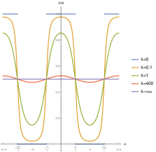
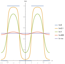
Figure 1: The positive and negative branches of $\lambda(\alpha)$ in Eq. (24) are plotted for different values of $k$.

Then, with the change of variable in Eq. (24), our task has been reduced to solving a single ODE for $\alpha(r)$ in Eq. (25). Interestingly enough, such an ODE is solvable since it can be reduced to the following quadrature

$$\left[\frac{\sin^{2}(\alpha)}{2(\cos^{2}(\alpha)+k)^{3}}\right]\alpha^{\prime 2}=E_{0}\ \ ,$$ (26)

$$\frac{d\alpha}{\rho\left(\alpha,E_{0}\right)}=\pm dr\ ,\qquad\rho\left(\alpha,E_{0}\right)=\frac{\left(2E_{0}\right)^{1/2}(\cos^{2}(\alpha)+k)^{3/2}}{\sin(\alpha)}\ ,$$ (27)

where $E_{0}$ is an integration constant. Moreover, Eq. (25) (or, equivalently, Eq. (27)) can be solved explicitly, however, in order to compute all the relevant quantities such as the total energy, pressure and so on, the expression in Eq. (27) is sufficient.

Summarizing, the function $\alpha$, determined explicitly by the quadrature in Eqs. (26) and (27), in turn determines the dependence of $\lambda$ on $r$; through Eq. (24). These two functions are the analytic solutions of the $(2+1)$-dimensional Yang-Mills equations in Eqs. (21) and (22) on the cylinder defined in Eq. (6).

III.3 The energy of the condensate

The energy density $T_{00}$ (which in the case of the ansatz in Eq. (20) within the family of configurations defined in Eqs. (8), (9), (10) and (11)) reads

$$T_{00}=\frac{4p^{2}\left[4\lambda^{2}(\lambda-1)^{2}\alpha^{\prime 2}+\lambda^{\prime 2}\right]\sin^{2}(\alpha)}{e^{2}R^{2}L^{2}}\ .$$ (28)

When one takes into account that $\lambda$ depends on $\alpha$ as in Eq. (24) the energy density becomes

$$T_{00}=\frac{\xi}{\rho\left(\alpha,1\right)^{2}}\alpha^{\prime 2}\ ,$$ (29)

$$\rho\left(\alpha,1\right)=\rho\left(\alpha,E_{0}=1\right)\ ,\quad\xi=\frac{2\left(kp\right)^{2}(k+1)}{\left(LRe\right)^{2}}\ ,$$

where $\rho\left(\alpha,E_{0}\right)$ has been defined in Eq. (27). In this way, the total energy $E_{\text{tot}}$ of the system can be written as

$$E_{\text{tot}}=RL\int drd\phi T_{00}=2V_{c}\frac{E_{0}k^{2}(k+1)p^{2}}{e^{2}L^{2}R^{2}}\ ,$$ (30)

where $V_{c}$ is the cylinder volume defined in Eq. (7). It is worth to emphasize that these inhomogeneous gluonic condensates are non-perturbative, i.e., Eq. (30) is singular around $e=0$. Moreover, notice that the energy density turns out to be constant, and it depends on the parameter $k$ in Eq. (24) as well as on the integration constant $E_{0}$ in Eq. (26). $E_{0}$ is determined through the relation

$$r_{f}-r_{i}=\int_{\alpha(r_{i})}^{\alpha(r_{f})}\frac{1}{\rho(\alpha,E_{0})}d\alpha\ ,$$

once the boundary conditions are chosen, while the allowed values of $k$ can be calculated by requiring that the non-Abelian magnetic flux be quantized. We compute the non-Abelian magnetic flux in the next section for the most interesting case of the Georgi-Glashow model, this for two reasons that we detail here. The first reason is that the inclusion of the Higgs field allows to derive a BPS bound, from which a topological charge naturally emerges, and the non-triviality of this quantity determines the appropriate boundary conditions for the $\alpha$ profile. The second reason is that the non-Abelian magnetic flux, both for the case with Higgs field and without the Higgs, are actually the same. We detail more about these points in the next section.

IV Analytic non-homogeneous condensates in the Georgi-Glashow model

In this section, we construct non-homogeneous condensates in the Georgi-Glashow model. Thus, we set $\eta=1$ and $\mu=0$, in Eq. (1). As it has been already emphasized, in this model our ansatz is the one in Eq. (20) within the family of configurations defined in Eqs. (8), (9), (10), (11) and (12), and in the particular case when the Higgs field is

$$h=h(r)\ .$$ (31)

IV.1 Solving the field equations

The $(2+1)$-dimensional Georgi-Glashow field equations for the ansatz defined in Eqs. (6), (7), (8), (9), (10), (11), (12) and (31) reduce to the following three coupled non-linear ODEs for $\alpha(r)$, $\lambda(r)$ and $h(r)$:

$$\alpha^{\prime\prime}+\cot(\alpha)\alpha^{\prime 2}+\frac{3}{2}\frac{(2\lambda-1)}{\lambda(\lambda-1)}\lambda^{\prime}\alpha^{\prime}=\frac{e^{2}R^{2}}{4}\frac{\cot(\alpha)}{\lambda(\lambda-1)}h^{2}\ ,$$ (32)

$$\lambda^{\prime\prime}+2\lambda(\lambda-1)\tan(\alpha)\alpha^{\prime\prime}+2\left[2\cot(2\alpha)-\csc(2\alpha)+3\lambda\tan(\alpha)\right]\lambda^{\prime}\alpha^{\prime}-4\lambda\left(\lambda-1\right)^{2}\alpha^{\prime 2}=e^{2}R^{2}\lambda h^{2}\ ,$$ (33)

$$h^{\prime\prime}+\gamma R^{2}\left(vev^{2}-h^{2}\right)h=0\ .$$ (34)

We emphasize two remarkable features about the ansatz in Eq. (20), which is a generalization of the strategy developed in Refs. gaugsk , LastUS1 , LastUS2 for the Skyrme model. Firstly, although we have a non-trivial Higgs field, a direct computation shows that if $\lambda$ depends on $\alpha$, as in Eq. (24), then Eqs. (32) and (33) reduce again to just one ODE for $\alpha(r)$

$$\alpha^{\prime\prime}+\left[\cot\alpha+\frac{3\sin\alpha\cos\alpha}{\cos^{2}\alpha+k}\right]\alpha^{\prime 2}+\frac{e^{2}R^{2}}{k}\cot\alpha(\cos^{2}\alpha+k)h^{2}=0\ .$$ (35)

Moreover, the energy density becomes

$$T_{00}=\frac{p^{2}k^{2}(k+1)}{e^{2}R^{2}L^{2}}\frac{\sin^{2}(\alpha)}{(\cos^{2}(\alpha)+k)^{3}}\alpha^{\prime 2}+\frac{p^{2}(k+1)\cos^{2}(\alpha)}{L^{2}(\cos^{2}(\alpha)+k)}h^{2}+\frac{1}{2R^{2}}h^{\prime 2}+\frac{\gamma}{4}(vev^{2}-h^{2})^{2}\ .$$ (36)

Secondly, despite the facts that the ansatz is genuinely non-Abelian and that the commutators between the Higgs field and the gauge field as well as the commutators of the gauge field with itself are non-vanishing (see the Appendix), all the terms in the field equations for the Higgs field which could, in principle, couple the Higgs profile $h(r)$ with the gauge field profiles $\lambda(r)$ and $\alpha(r)$ actually vanish. The main technical reason behind this simplification is that the fields $\alpha$, $\Theta$ and $\Phi$ in Eq. (10) have been chosen in such a way that

$$\partial_{\mu}\alpha\partial^{\mu}\Phi=\partial_{\mu}\Theta\partial^{\mu}\Phi=\partial_{\mu}\Phi\partial^{\mu}\Phi=\partial_{\mu}h\partial^{\mu}\Phi=0\ .$$

This “decoupling property” is the Yang-Mills-Higgs generalization of the approach used in the gauged Skyrme model minimally coupled with the Maxwell field in gaugsk , LastUS1 , LastUS2 . Due to this decoupling property, Eq. (34) can be reduced to the following quadrature

$$\frac{\left(h^{\prime}\right)^{2}}{2}-\frac{\gamma R^{2}}{4}\left(h^{2}-vev^{2}\right)^{2}=\frac{I_{0}}{2}\qquad\Rightarrow\quad\pm dr\ =\frac{dh}{\sqrt{I_{0}+\frac{\gamma R^{2}}{2}\left(h^{2}-vev^{2}\right)^{2}}}\ ,$$ (37)

where $I_{0}$ is an integration constant. Consequently, one can solve explicitly the Higgs field in Eq. (34) (or equivalently in Eq. (37)) in terms of a Jacobi elliptic function, that is

$$h(r)=K_{0}\mathrm{sn}(u(r)-u_{0},\kappa)\ ,$$ (38)

with

$$K_{0}=\kappa\sqrt{\frac{2}{\kappa^{2}+1}}vev\ ,\quad\text{and}\quad u(r)=\frac{K_{0}}{\kappa}\sqrt{\frac{\gamma}{2}}Rr\ .$$ (39)

In the previous equations, the integration constants $u_{0}$ and $\kappa$ correspond to the phase and the elliptic modulus, respectively. Without any loss of generality, we can fix $u_{0}=0$ because it just corresponds to a shift in the $r$ coordinate and can be absorbed into a coordinate’s redefinition. Moreover, inserting Eqs. (38) and (39) into (37) yields

$$I_{0}=-\frac{\gamma R^{2}(vev)^{4}(1-\kappa^{2})^{2}}{2(1+\kappa^{2})^{2}},$$ (40)

which makes manifest that $\kappa=1$ corresponds to $I_{0}=0$.

Therefore, we have reduced the problem to solve the three coupled non-linear ODEs in Eqs. (32), (33) and (34) to solve only Eq. (35), where $h$ is explicitly known. Notice that there are three types of possible solutions for the Higgs field. The simplest non-trivial solution corresponds to taking the profile $h=\pm vev$ in Eq. (34). The second option is to consider a non-constant solution of Eq. (37) with $I_{0}=0$ (or $\kappa=1$ in Eq. (38)), which corresponds to a kink-type solution. Otherwise, for $I_{0}\neq 0$ in Eq. (37) the solution is periodic. We consider these three possibilities in separate sub-sections.

At this point it is important to emphasize that despite the dramatic simplification of the field equations that we have previously shown, the configurations constructed here are genuinely non-Abelian. Indeed, not only many of the commutators between the gauge potential and the Higgs fields are non-vanishing (see the Appendix), but also one can see that meron-type configurations (which only appear in non-Abelian gauge theories) are a particular case of the present family of configurations; cf. Eq. (11) and the comments below it.

IV.2 Constant Higgs profile

In this subsection we consider $h=\pm vev$, for which Eq. (35) becomes

$$\alpha^{\prime\prime}+\left[\cot\alpha+\frac{3\sin\alpha\cos\alpha}{\cos^{2}\alpha+k}\right]\alpha^{\prime 2}+\frac{e^{2}R^{2}\left(vev\right)^{2}}{k}\cot\alpha(\cos^{2}\alpha+k)=0\ ,$$ (41)

while, the Higgs equation in Eq. (34) is automatically satisfied. Quite interestingly, the above equation can be reduced to a quadrature since Eq. (41) possesses the following first integral:

$$\left[\frac{\sin^{2}\alpha}{2(\cos^{2}\alpha+k)^{3}}\right]\alpha^{\prime 2}+\frac{e^{2}R^{2}\left(vev\right)^{2}}{2k(\cos^{2}\alpha+k)}=E_{0}\ ,$$ (42)

where $E_{0}$ is an integration constant. Thus, the complete set of field equations of the Georgi-Glashow model can be reduced to the following quadrature:

$$\frac{d\alpha}{\rho\left(\alpha,E_{0}\right)}=\pm dr\ ,\qquad\rho\left(\alpha,E_{0}\right)=\frac{\cos^{2}{\alpha}+k}{\sin{\alpha}}\sqrt{2(\cos^{2}{\alpha}+k)E_{0}-\frac{e^{2}R^{2}(vev)^{2}}{k}}\ .$$ (43)

We also mention that the above quadrature can be explicitly solved in terms of generalized elliptic integrals (see Elliptics ), although, one can compute analytically relevant physical quantities, such as the energy and the pressure, just using Eq. (43), as shown below.

IV.2.1 Energy density and BPS bound

The energy density in Eq. (36) with $h=\pm vev$ is reduced to

$$T_{00}=\frac{p^{2}(k+1)}{L^{2}}\left[\frac{k^{2}\sin^{2}(\alpha)}{e^{2}R^{2}(\cos^{2}(\alpha)+k)^{3}}\alpha^{\prime 2}+\frac{\left(vev\right)^{2}\cos^{2}(\alpha)}{\cos^{2}(\alpha)+k}\right]\ .$$ (44)

A very relevant feature of the above expression for the energy density and, in fact, of the full energy-momentum tensor, is that it has the right periodicity in $\phi$. In particular, we remind the reader that, in the case of gauge theories, one has to require that physical gauge-invariant observables (such as the energy density) must be periodic functions of $\phi$. However, the gauge potential itself (which is not gauge-invariant) need not be so.

In this case, it is possible to derive a non-trivial BPS bound rewriting $T_{00}$ as

$$T_{00}=\frac{p^{2}(k+1)}{L^{2}}\left[\left(\varsigma\left(\alpha\right)\alpha^{\prime}\pm W\left(\alpha\right)\right)^{2}\mp 2\varsigma\left(\alpha\right)W\left(\alpha\right)\alpha^{\prime}\right]\ ,$$ (45)

$$\varsigma\left(\alpha\right)=\frac{k\sin(\alpha)}{eR(\cos^{2}(\alpha)+k)^{3/2}}\ ,\quad W\left(\alpha\right)=\frac{\left(vev\right)\cos(\alpha)}{\left(\cos^{2}(\alpha)+k\right)^{1/2}}\ .$$ (46)

Consequently (since the term $2\varsigma\left(\alpha\right)W\left(\alpha\right)\alpha^{\prime}$ in Eq. (45) is a total derivative), the following BPS bound on the total energy, defined in Eq. (30), can be derived

$$E_{\text{tot}}\geq\left|Q^{H}\right|\ ,$$ (47)

where the topological charge is given by

$$Q^{H} =\pm\frac{p^{2}(k+1)}{L^{2}}\times 2\pi RL\int_{r_{i}}^{r_{f}}2\varsigma\left(\alpha\right)W\left(\alpha\right)\frac{d\alpha}{dr}dr\$$

$$=\pm\left.\frac{2\pi p^{2}k(k+1)vev}{e\,L\,(\cos^{2}\alpha+k)}\right|_{\alpha(r_{i})}^{\alpha(r_{f})}\ .$$ (48)

The above bound can be saturated if and only if the following first order equation is satisfied:

$$\varsigma\left(\alpha\right)\alpha^{\prime}=\pm W\left(\alpha\right)\ .$$ (49)

It is a very non-trivial result that in the presence of a Higgs field the BPS condition, here above, implies that the second order field equation in Eq. (41) is satisfied.

Notice that the first-order equations in Eqs. (42) and (49) are compatible for a particular value of the integration constant $E_{0}$, namely

$$E_{0}\ =\ \frac{e^{2}R^{2}(vev)^{2}}{2k^{2}}\ .$$

While the solutions of the equation that comes from the saturation of the BPS bound in Eq. (49) only correspond to a set of all the allowed solutions of Eq. (41), all solutions of Eq. (41) are also solution of Eq. (42). Therefore, though the existence of a BPS bound that allows to solve the Yang-Mills-Higgs system analytically is something clearly non-trivial, throughout the paper we do not refer to the solutions that can be obtained from Eq. (49), but rather to those general solutions of Eq. (41) (or equivalently Eq. (42)).

IV.2.2 Boundary conditions and topological charge

Evaluating the topological charge in Eq. (49) at the top and the bottom of the cylinder in the range defined in Eq. (7) we see that, in order to have a non-vanishing topological charge, we must demand that, $\cos^{2}{\alpha(r_{i})}\neq\cos^{2}{\alpha(r_{f})}$. Then, suitable boundary conditions for the $\alpha$ profile are

$$\alpha(r_{i})=\frac{\pi}{2}\ ,\qquad\alpha(r_{f})=0\ .$$ (50)

In fact, with the above boundary conditions the topological charge becomes

$$Q^{H}=\pm\frac{2\pi p^{2}(vev)}{eL}\ .$$ (51)

Note that the appropriate boundary conditions for the $\alpha$ profile can be read directly from Eq. (43). Indeed, as we are looking for regular solutions it is necessary that $\alpha^{\prime}$ must not have singularities or change sign, and this implies that $\alpha$ can only be extended in a length range from $0$ to $\frac{\pi}{2}$. Now, the integration constant $E_{0}$ is fixed through the relation

$$r_{f}-r_{i}=\pm\int_{0}^{\frac{\pi}{2}}\frac{1}{\rho(\alpha,E_{0})}d\alpha\ ,$$

with $\rho(\alpha,E_{0})$ defined in Eq. (43).

To the best of the authors’ knowledge, the topological charge in Eqs. (47), (48) and (51) is novel, non-trivial and useful. First of all, it is novel since $Q^{H}$ does not coincide with the non-Abelian magnetic flux or the enclosed electric charge which, usually, play the role of topological charges in non-Abelian gauge theories. It is non-trivial since we can construct solutions with non-vanishing $Q^{H}$. It is useful since the requirement to saturate the BPS bound in Eq. (47) gives rise to a first order condition, which implies the second order field equations. These results are likely to be genuine finite density effects and are, consequently, very relevant when analyzing the theory within a finite volume.

IV.3 Non-constant Higgs profile: The general case

Not surprisingly, the case in which the Higgs profile is non-constant is considerably more difficult. Nevertheless, many analytic results can be derived. The field equation for the profile $\alpha$ in this case is given by

$$\alpha^{\prime\prime}+\left[\cot\alpha+\frac{3\sin\alpha\cos\alpha}{\cos^{2}\alpha+k}\right]\alpha^{\prime 2}+\frac{e^{2}R^{2}}{k}\cot\alpha(\cos^{2}\alpha+k)h^{2}=0\ ,$$ (52)

where $h$ is a non-constant solution of Eq. (37) defined in general in Eq. (38). In order to simplify the above equation it is useful to introduce a new function of $\alpha$, which we denote by $\Gamma\left(\alpha\right)$, and is defined by the following relation:

$$\frac{d\Gamma\left(\alpha\right)}{dr}=\mp\left[\frac{\sin(\alpha)}{2(\cos^{2}(\alpha)+k)^{3/2}}\right]\alpha^{\prime}\qquad\Rightarrow\quad\Gamma\left(\alpha\right)=\pm\frac{\cos(\alpha)}{2k\sqrt{\cos^{2}(\alpha)+k}}\ ,$$ (53)

so that the profile $\alpha$ can be written as

$$\alpha=\arccos\left[\biggl{(}\frac{k\Gamma^{2}}{\frac{1}{4k^{2}}-\Gamma^{2}}\biggl{)}^{\frac{1}{2}}\right]\ .$$ (54)

Then one is left with the following simpler linear equation

$$\Gamma^{\prime\prime}-(e^{2}R^{2}h^{2})\Gamma=0\ .$$ (55)

Notice that by examining Eq. (53) and comparing it with Eq. (24), the above $\Gamma(\alpha)$ function is proportional to our earlier defined $\lambda(\alpha)$ function

$$\Gamma=\frac{2\lambda-1}{2k}\ .$$ (56)

From Eq. (54), the complete set of field equations of the Georgi-Glashow model with a non-constant Higgs profile has been reduced to just Eq. (55) where $h$ is a non-constant solution of Eq. (37).

IV.3.1 Mapping with the Lamé equation

We now move on to solving the only pending ODE to have a complete solution of the Georgi-Glashow field equations. Let us recall that the non-constant Higgs profile obeys Eq. (37). In that equation, the integration constant $I_{0}$ characterizes the configurations period determined by $\kappa$, and the general solution is an elliptic sine function as showed in Eq. (38). In this case, the system can be taken to solve a Lamé equation.

Notice that Eq. (38) is at its simplest in terms of the variable $u$ defined in Eq. (39). Thus, we transform Eq. (55) by considering

$$y(u)=\Gamma(r(u))\ ,$$ (57)

so that it becomes

$$\frac{\mathrm{d}^{2}y}{\mathrm{d}u^{2}}-l(l+1)\kappa^{2}\mathrm{sn}^{2}(u,\kappa)\,y=0\ ,$$ (58)

where $l$ has been defined so that it satisfies $l(l+1)=2e^{2}/\gamma$, for which there are always solutions. This combination of the coupling constants $e$ and $\gamma$ is always positive and so leads to real values of $l$.

The ODE in Eq. (58) is known as the Lamé equation and its solutions as Lamé functions. Special situations arise when $l$ is an integer, however, solutions always exist for general complex values of $l$, that would be acceptable to us. It is well-known that the Lamé functions are a special case of Heun functions. We write the general solution of Eq. (58) as

$$y(u)=c_{1}\,H\left(\frac{1}{\kappa^{2}},0,-\frac{l}{2},\frac{l+1}{2},\frac{1}{2},\frac{1}{2},\mathrm{sn}^{2}{u}\right)+c_{2}\,\mathrm{sn}{u}\,H\left(\frac{1}{\kappa^{2}},\frac{1+\kappa^{2}}{4\kappa^{2}},\frac{l+2}{2},\frac{1-l}{2},\frac{3}{2},\frac{1}{2},\mathrm{sn}^{2}{u}\right)\ ,$$ (59)

where every elliptic function has the same elliptic modulus $\kappa$ (we have omitted them for simplicity). Moreover, $H$ denotes a general Heun function $H(a,q,\alpha,\beta,\gamma,\delta,z)$ which satisfies the equation (see Heun )

$$\frac{d^{2}w}{dz^{2}}+\left[\frac{\gamma}{z}+\frac{\delta}{z-1}+\frac{\epsilon}{z-a}\right]\frac{dw}{dz}+\frac{\alpha\beta z-q}{z(z-1)(z-a)}w=0\ ,$$ (60)

where $\epsilon=\alpha+\beta-\gamma-\delta+1$. Let us note that for both Heun functions in Eq. (59) $\epsilon=1/2$.

Before continuing, we recall that Jacobi elliptic functions are doubly-periodic; they have a real and an imaginary period. For Lamé functions to be doubly-periodic $l$ must be an integer. However, for any value of $l$, integer or not, there are infinitely many solutions with real period $2K$ or $4K$, where $K$ denotes the quarter period integral which is a function of $\kappa$, the elliptic modulus, i.e.,

$$K(\kappa)=\int_{0}^{\pi/2}\frac{\mathrm{d}\varpi}{\sqrt{1-\kappa^{2}\sin^{2}\varpi}}\ .$$ (61)

Henceforth, we fix the integration constant $\kappa$ in terms of the length of the space-time cylinder by

$$r_{f}-r_{i}=2K(\kappa)\ .$$ (62)

IV.4 Non-constant Higgs profile: The kink case

In the previous section, we showed that for non-constant Higgs profiles solving the complete Georgi-Glashow model field equations leads generically to a Lamé equation. However, a very special case arises when in Eq. (37) one considers $I_{0}=0$ or, equivalently $\kappa=1$ in Eq. (38). In this case, the Higgs profile becomes a kink

$$h(u)=vev\tanh u\ ,$$ (63)

as can be seen from equations Eqs. (38) and (39). Notice that the kink is asymptotically constant, i.e., when $u\to\pm\infty$ then $h(u)\to\pm vev$. Thus, the kink case is connected to both of our previously examined cases, constant and non-constant profiles.

IV.4.1 Mapping with the Pöschl-Teller equation

Evaluating Eq. (58) at $\kappa=1$ yields

$$\frac{\mathrm{d}^{2}y}{\mathrm{d}u^{2}}-l(l+1)\tanh^{2}(u)\,y=0\ ,$$ (64)

which can be written as

$$-\frac{1}{2}\frac{\mathrm{d}^{2}y}{\mathrm{d}u^{2}}-\frac{l(l+1)}{2}\mathrm{sech}^{2}(u)\,y=-\frac{l(l+1)}{2}y\ .$$ (65)

This is a one-dimensional Schrödinger equation with a Pöschl-Teller potential (see barut ). The solutions of which are known to be Legendre functions of the form $P^{\nu}_{l}(\tanh(u))$. However, just as Eq. (58) is not the most general Lamé equation also Eq. (65) is not the most general Pöschl-Teller equation. In this case, we are restricted by

$$\nu^{2}=l(l+1)\ .$$ (66)

Notice that as $u\to\pm\infty$ then $\tanh(u)\to\pm 1$. This is problematic for us as Legendre functions are generically singular at the points $(-1,1,\infty)$. In Quantum Mechanics this issue is resolved by quantization conditions on $l$ and $\nu$. These conditions guarantee that the Legendre functions vanish at the boundary, as they are interpreted as wave functions. However, under our current restriction we can only employ one quantization condition. As a consequence, solutions $y(u)$ can be regular only at plus or minus infinity, but not both.

From its definition in Eq. (53), we see that $\Gamma(\alpha)$ is bounded from above, which also applies for $y(u)$. This is incompatible with the Legendre functions in the general solution of Eq. (65). To resolve this issue, we consider the space-time cylinder as semi-infinite, meaning

$$0<r<\infty\ ,$$ (67)

where we fix the origin at the bound of $y(u)$. The solutions

$$y(u)=P^{\sqrt{n(n+1)}}_{n}(-\tanh u)\ ,$$ (68)

all fulfill our desiderata whenever $n$ is an integer.

It is interesting to note that when the Chern-Simons term is included (see Section 6) it is natural to expect that only semi-infinite cylinders are allowed since the Chern-Simons coupling introduces exponential terms which decay in one direction but not in the other. What is slightly surprising is that a similar behavior is also present without the Chern-Simons term. In a sense, in the limit in which the cylinder has an infinite volume, the theory feels the presence of the Chern-Simons term even if it is not included directly in the action.

IV.5 Non-Abelian magnetic flux

Now we discuss the resulting non-Abelian flux. First, being in a cylinder, it is clear that we should require periodic boundary conditions in the $\phi$ direction (with period $2\pi$) for the non-Abelian field strength and for the energy-momentum tensor. As we mentioned before, the ansatz in Eq. (20) automatically satisfies this condition for $p$ an integer number. One can check directly that the flux in Eq. (5) for the configurations defined by the ansatz in Eqs. (8), (9), (10), (11) and (20) is given by

$$\Psi^{1}_{\text{M}}=\Psi^{2}_{\text{M}}=0\ ,\quad\quad\Psi^{3}_{\text{M}}=\int dr\chi(r)\ ,$$ (69)

where

$$\chi(r)=-2kp\pi\frac{\sin(\alpha)(\sin^{2}(\alpha)+\cos(\alpha)\sqrt{k+\cos^{2}(\alpha)})}{(k+\cos^{2}(\alpha))^{\frac{3}{2}}}\alpha^{\prime}\ ,$$ (70)

and we have integrated in the coordinate $\phi$ and used the relation $\lambda=\lambda(\alpha)$ in Eq. (24).

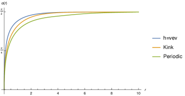
Figure 2: The regular $\alpha$ profiles for the solutions with constant Higgs, the kink case and the periodic case for the boundary conditions in Eq. (50). Here we have considered $e=\gamma=vev=1$, $R=L=p=1$, $k=0.2736$ and $\kappa=1/2$ for the periodic solution.

It is important to note that the non-Abelian flux is the same for all the configurations constructed here, that is with and without a Higgs field. Although in the Georgi-Glashow model the Higgs field $h$ is implicit in the solutions for the profile $\alpha$ (see for instance Eq. (43)), the final expression for the non-Abelian flux does not depend on $h$ since the integration can be carried out in $\alpha$ instead of the $r$ coordinate. This is due to the fact that the integrand that appears in the non-Abelian flux in Eq. (70) has a global factor $\alpha^{\prime}$.

Now, considering the boundary conditions in Eq. (50), the non-null non-Abelian magnetic flux turns out to be

$$\Psi^{3}_{\text{M}}=\frac{p\pi}{\sqrt{k+1}}\biggl{(}2+2k+k\sqrt{k+1}\log(k+1)-2k\sqrt{k+1}\log(\sqrt{k+1}+1)\biggl{)}\ .$$

Imposing the condition of a quantized magnetic flux, that is

$$\Psi^{3}_{\text{M}}=np\ ,\qquad\text{with}\quad n\in\mathbb{Z}\ ,$$ (71)

we get to the following (first) allowed values of the $k$ constant:

$$k_{1}=19.4003\ ,\quad k_{2}=2.62628\ ,\quad k_{3}=0.273648\ ,\quad k_{4}=-0.42079\ ,\quad k_{5}=-0.698148\ ,$$

$$k_{6}=-0.828956\ ,\quad k_{7}=-0.897471\ ,\quad k_{8}=-0.936029\ ,\quad k_{9}=-0.958882\ .$$

Notice that in our convention (see Eqs. (1) through (4)) the Yang-Mills coupling constant $e$, appears in the action and not in front of commutators. In the alternative convention, magnetic flux is not dimensionless and the equivalent of Eq. (71) is a quantization in terms of $1/e$.

With the set of values for $k$ displayed above, we can now plot some relevant physical quantities. In Fig. 2 we show the $\alpha$ profile for all the cases when the Higgs field is present. We can see that in all these cases, we are able to obtain regular solutions for the boundary conditions in Eq. (50) imposed by the condition of a non-vanishing topological charge. In Fig. 3 we show the profile, the $\Gamma$ function, the energy density and the $\chi$ function in the non-Abelian flux for the three cases in the Georgi-Glashow model. We see that in all the cases the energy as well as the non-Abelian flux are concentrated at the origin of the cylinder. In Fig. 4 we show that finite density transitions exist between the two configurations of finite height, namely the constant Higgs case and the periodic case, and this transition depends on the length of the tube in which the condensate is confined. For large values of the volume of the cylinder the energetically favored configuration is the one with a constant Higgs profile, while, for small volumes is the periodic case. Note that it makes sense to compare the energy of these configurations since both configurations have the same magnetic flux, as can be seen from Eqs. (69) and (70).

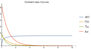
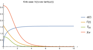
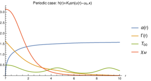
Figure 3: Behavior of $\alpha(r)$ and $\Gamma(r)$ profiles as well as the energy density and the non-Abelian density flux for the solutions with constant Higgs, the kink case and the periodic case. Here we have considered $e=\gamma=vev=1$, $R=L=p=1$, $k=0.2736$ and $\kappa=1/2$ for the periodic solution.

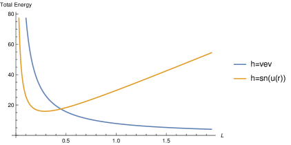
Figure 4: Energy comparison between the solutions with finite height. The length of the tube in which the condensate is confined determines that for large values of the volume of the cylinder the energetically favored configuration is the one with a constant Higgs profile, while, for small volumes is the one with the Higgs profile given by $h(r)=K_{0}{\rm sn}(u,\kappa)$.

V Small fluctuations and stability

In this section, we analyze the linearized Yang-Mills-Higgs equation on the non-homogeneous condensate constructed in the previous sections. Since the full stability analysis of the non-homogeneous condensates is extremely complicated even from the numerical viewpoint (as one should analyze a coupled system of twelve partial differential equations in a non-trivial background solution) we consider here the simplest non-trivial perturbations which are under some analytic control. It is worth emphasizing that the linear stability analysis in the present section only concerns the behavior of the analytic solutions constructed in the previous sections under small perturbations. Consequently, in the present section the term ”stable” actually means linearly stable. The situation should be contrasted with BPS solutions which are stable also at non-linear level. This family of perturbations of the Yang-Mills and Higgs profiles are

$$h(r)\ \longrightarrow\ h(r)+\epsilon P_{1}(r)\ ,$$ (72)

$$\Gamma(r)\ \longrightarrow\ \Gamma(r)+\epsilon P_{2}(r)\ ,$$ (73)

with $\epsilon\ll 1$. The fluctuation’s operator $\widehat{O}$ corresponding to the perturbations defined above is:

$$\widehat{O}\left(\begin{array}[]{c}P_{1}\\ P_{2}\end{array}\right)=\left(\begin{array}[]{c}-\frac{d^{2}P_{1}}{dr^{2}}+\gamma R^{2}(3h^{2}-vev^{2})P_{1}\\ -\frac{d^{2}P_{2}}{dr^{2}}+e^{2}R^{2}h^{2}P_{2}+2e^{2}R^{2}h\Gamma P_{1}\end{array}\right)\ .$$ (74)

Therefore, a necessary condition for stability is that the operator $\widehat{O}$ should only possess non-negative eigenvalues. Thus, we analyze the linear equations here below

$$-\frac{d^{2}P_{1}}{dr^{2}}+\gamma R^{2}(3h^{2}-vev^{2})P_{1} =EP_{1}\ ,$$ (75)

$$-\frac{d^{2}P_{2}}{dr^{2}}+e^{2}R^{2}h^{2}P_{2}+2e^{2}R^{2}h\Gamma P_{1} =EP_{2}\ ,$$ (76)

and we discuss in which of the cases discussed above $E$ is non-negative. The proper boundary conditions in the $r$ coordinate for the perturbations $P_{1}$ and $P_{2}$ must be chosen in such a way that the topological charge and the non-Abelian magnetic flux must not change at order $\epsilon$ (otherwise $P_{1}$ and $P_{2}$ would not be small perturbations). Eq. (76) shows that it is convenient to solve Eq. (75) first.

V.1 Radial perturbations of the condensates with constant Higgs profile

Let us begin by considering a constant Higgs profile $h=\pm vev$ in a tube of finite size. In this case, Eq. (75) becomes

$$P_{1}^{\prime\prime}+\omega_{1}^{2}P_{1}=0\ ,$$ (77)

where

$$\omega_{1}^{2}=E-2\gamma R^{2}vev^{2}.$$ (78)

Indeed, if $\omega_{1}^{2}$ is not positive, then the perturbation $P_{1}$ could not satisfy periodic boundary conditions in $r$ (on the other hand, when $P_{1}$ satisfies periodic boundary conditions, the topological charge and the non-Abelian magnetic flux do not change at order $\epsilon$). Consequently, we must have $E>2\gamma R^{2}vev^{2}$, so that the necessary condition for stability discussed above is satisfied.

Now that we have established that radial perturbations of the profile are harmonic, we move on to Eq. (76) which requires we know both $P_{1}(r)$ and $\Gamma(r)$. By proceeding as above we find that

$$P_{2}^{\prime\prime}+\omega_{2}^{2}P_{2}=F(r)\ ,$$ (79)

which is the equation of an undamped driven harmonic oscillator whose angular frequency is

$$\omega_{2}^{2}=E-e^{2}R^{2}vev^{2}\ .$$ (80)

The driving force is partly described by $P_{1}$, which is sinusoidal, and by $\Gamma$ which for constant $h=\pm vev$ is exponential; see Eq. (55). Concretely, the driving force is

$$F(r)=e^{\pm eR(vev)r}(A\cos(\omega_{1}r)+B\sin(\omega_{1}r))\ ,$$ (81)

where $A$ and $B$ are fixed by the boundary conditions for $\Gamma$ and $P_{1}$.

The general solution of Eq. (79) is

$$P_{2}=C_{1}\cos(\omega_{2}r)+C_{2}\cos(\omega_{2}r)+\frac{e^{eRhr}[(A\gamma hR-Be\omega_{1})\cos(\omega_{1}r)+(B\gamma hR+Ae\omega_{1})\sin(\omega_{1}r)]}{2hR(e^{2}\omega_{1}^{2}+\gamma^{2}R^{2}h^{2})}\ ,$$ (82)

where $h=\pm vev$ in this case. Notice that perturbations never explode as the denominator of the particular solution is always positive. By choosing boundary conditions for $P_{2}$ such that vanishes at both ends of the tubes, we fix the integration constants $C_{1}$ and $C_{2}$ in terms of $A$ and $B$. This choice guarantees that the charges do not change with the perturbation.

V.2 Radial perturbations of the condensates with non-constant Higgs profile

When the Higgs profile is not constant then radial perturbations become quite unmanageable. However, for the semi-infinite kink case we mention the following. Carrying out the change of variable in Eq. (39) allows for Eq. (75) to be written as

$$-\frac{\mathrm{d}^{2}p_{1}}{\mathrm{d}u^{2}}+6\kappa^{2}\mathrm{sn}^{2}(u,\kappa)\,p_{1}=\tilde{E}p_{1}\ ,$$ (83)

where $P_{1}(r(u))=p_{1}(u)$ and

$$\tilde{E}=\frac{\kappa^{2}+1}{\gamma R^{2}(vev)^{2}}\left[E+\gamma R^{2}(vev)^{2}\right]\ .$$ (84)

One can see that the perturbation is governed by a Lamé equation with $l=2$, and whose general solution is given in terms of Heun functions. For the semi-infinite kink case (that is, setting $\kappa=1$), Eq. (83) becomes a Pöschl-Teller equation:

$$-\frac{\mathrm{d}^{2}p_{1}}{\mathrm{d}u^{2}}-6\mathrm{sech}^{2}(u)\,p_{1}=\left[-4+\frac{2E}{\gamma R^{2}(vev)^{2}}\right]p_{1}\ .$$ (85)

In this case, using known results on the Pöschl-Teller equation barut one can show that $E\geq 0$, so that also in this case the non-homogeneous condensate is stable under the perturbation defined here above.

VI Analytic non-homogeneous condensates in the Yang-Mills-Higgs-Chern-Simons theory

In previous sections, we have seen that Eq. (24) is applicable for both constant and non-constant Higgs profiles. Remarkably, when the Yang-Mills-Higgs action is additionally coupled to Chern-Simons theory the equations of motion are still compatible with our general approach, as shown below.

Also in this case, for the ansatz defined in Eqs. (8), (9), (10), (11), (12) and (20) together with the relation between $\lambda$ and $\alpha$ in Eq. (24), the complete set of Yang-Mills-Higgs-Chern-Simons field equations in Eqs. (3) and (4) are reduced to just one equation for the soliton profile, that is

$$\alpha^{\prime\prime}+\left[\cot\alpha+\frac{3\sin\alpha\cos\alpha}{\cos^{2}\alpha+k}\right]\alpha^{\prime 2}+\frac{e^{2}R^{2}h^{2}}{k}\cot\alpha(\cos^{2}\alpha+k)-\mu R\alpha^{\prime}=0\ ,$$ (86)

while, the Higgs potential $h(r)$ has the general solution in Eq. (38).

As we did before, this equation can be simplified by using the change in Eqs. (53) and (54) leading to the generalization of Eq. (55):

$$\Gamma^{\prime\prime}-(e^{2}R^{2}h^{2})\Gamma-\mu R\Gamma^{\prime}=0\ .$$ (87)

As the Higgs profile $h$ acquires its simplest form in terms of the variable $u$, cf. Eq. (39), we make this change and arrive at

$$\frac{\mathrm{d}^{2}y}{\mathrm{d}u^{2}}-l(l+1)\kappa^{2}\mathrm{sn}^{2}(u)y-m\sqrt{1+\kappa^{2}}\frac{\mathrm{d}y}{\mathrm{d}u}=0\ ,$$ (88)

where $m=\frac{\mu}{vev\sqrt{\gamma}}$ and $l(l+1)=\frac{2e^{2}}{\gamma}$, as defined earlier. By reparameterizing $y$ as

$$y(u)=e^{\frac{m}{2}\sqrt{1+\kappa^{2}}u}Y(u)\ ,$$ (89)

we see that $Y(u)$ is a Lamé function, as it satisfies

$$\frac{\mathrm{d}^{2}Y}{\mathrm{d}u^{2}}-l(l+1)\kappa^{2}\mathrm{sn}^{2}(u)Y-\frac{1}{4}m^{2}(1+\kappa^{2})Y=0\ .$$ (90)

Moreover, when $\kappa=1$ we have a Pöschl-Teller equation

$$-\frac{1}{2}\frac{\mathrm{d}^{2}Y}{\mathrm{d}u^{2}}-\frac{l(l+1)}{2}\mathrm{sech}^{2}(u)Y=-\frac{1}{2}\left[l(l+1)+\frac{1}{2}m^{2}\right]Y\ .$$ (91)

We also remark that, similar to the case $m=0$, of previous sections, desired solutions on a semi-infinite space-time cylinder are obtained by integer values of $l$. Interestingly enough, $m$ can take arbitrary values. In other words,

$$y(u)=e^{\frac{m}{\sqrt{2}}u}P_{n}^{\sqrt{n(n+1)+m^{2}/2}}(-\tanh u)\ ,$$ (92)

where $m$ is real but $n$ is an integer and $P$ is a Legendre function. To the best of the authors’ knowledge, this is the first family of analytic topologically non-trivial solutions of non-homogeneous condensates in the Yang-Mills-Higgs-Chern-Simons theory. We analyze the physical properties of these solutions in a forthcoming paper. Here, we only remark that, due to the presence of the Chern-Simons term, the factor $e^{\frac{m}{\sqrt{2}}u}$ (which appears in the solution here above) is well-defined either on finite intervals or (if one is interested in the infinite volume limit) when $-\infty<u\leq 0$. Hence, in the case in which the Chern-Simons coupling is included, one can only have semi-infinite tubes.

VII Conclusions

Using a non-spherical generalization of the usual hedgehog ansatz, the first analytic examples of non-homogeneous condensates, both in the $(2+1)$-dimensional Georgi-Glashow model as well as in the Yang-Mills-Higgs-Chern-Simons theory at finite density have been constructed. These exact configurations live within a cylinder which can have either finite height or can be infinitely long on one side, being the maximum of the energy density located at the origin of the tube. These non-homogeneous condensates possess a (novel) non-trivial topological charge, in such a way that the condensates cannot decay into the trivial vacuum. Such charge does not coincide with the non-Abelian magnetic flux, which usually plays the role of the topological charges in gauge theories. Requiring the quantization of the non-Abelian flux one of the free parameters characterizing the ansatz for the non-Abelian gauge field can be fixed. We show that depending on the length of the cylinder, finite density transitions occur. In particular, for large values of $L$ the energetically favored configuration is the one with a constant Higgs profile, while, for small values is the one with the Higgs profile given by an elliptic function. Also, we have derived some necessary conditions in order to have stable condensates under radial perturbations. These surprising results open the possibility to study the dynamics of Quarks moving in these topologically non-trivial condensates with analytic tools. We hope to come back on this important issue in a future publication.

Acknowledgments

F. C. has been funded by Fondecyt Grants 1200022. M. L. is funded by FONDECYT post-doctoral Grant 3190873. A.V. is funded by FONDECYT post-doctoral Grant 3200884. D.F. is supported by a CONACYT postdoctoral fellowship. This work has been partially funded by CONACYT Grant No. A1-S-11548. The Centro de Estudios Científicos (CECs) is funded by the Chilean Government through the Centers of Excellence Base Financing Program of Conicyt.

VIII Appendix: Some useful tensors

In this Appendix, we explicitly show some quantities that help to clarify the construction of our analytic solutions starting from the ansatz in Eqs. (6), (7), (8), (9), (10), (11), (12) and (20).

First of all, the matrices $U$ and $\varphi$ are explicitly given by

$$U=\begin{pmatrix}\cos(\alpha)&ie^{-i\Phi}\sin(\alpha)\\ ie^{i\Phi}\sin(\alpha)&\cos(\alpha)\end{pmatrix}\ ,\qquad\varphi=\begin{pmatrix}0&ie^{-i\Phi}h(r)\\ ie^{i\Phi}h(r)&0\end{pmatrix}\ .$$

For the computation of relevant physical quantities, it is convenient to define the following functions

$$f_{1}(r)\ =\ -2\cos(\alpha)\alpha^{\prime}(\lambda-1)\lambda+\sin(\alpha)\lambda^{\prime}\ ,$$

$$f_{2}(r)\ =\ 2\sin(\alpha)\alpha^{\prime}(\lambda-1)\lambda+\cos(\alpha)\lambda^{\prime}\ ,$$

and also

$$g_{1}(r)\ =\ 2\sin^{2}(\alpha)\lambda-1\ ,$$

$$g_{2}(r)\ =\ \sin(\alpha)\lambda\ .$$

From the above, one can check that the non-vanishing components of the non-Abelian field strength are

$$F_{tr}=p\begin{pmatrix}-if_{1}(r)&-e^{-i\Phi}f_{2}(r)\\ e^{i\Phi}f_{2}(r)&if_{1}(r)\end{pmatrix}\sin(\alpha)\ ,\qquad F_{r\phi}=LF_{tr}\ .$$

The non-Abelian character of our solutions is made manifest by non-null commutators that appear in the field equations in Eqs. (3) and (4). Indeed, by defining the following tensors

$$P^{\mu}=[A_{\nu},F^{\mu\nu}]\ ,$$

$$J^{\mu}=[\varphi,D^{\mu}\varphi]\ ,$$

a direct calculation shows that

$$P^{t}=\frac{2p}{L}\begin{pmatrix}-if_{2}(r)&e^{-i\Phi}f_{1}(r)\\ -e^{i\Phi}f_{1}(r)&if_{2}(r)\end{pmatrix}\sin(\alpha)\alpha^{\prime}\ ,\qquad P^{\phi}=\frac{1}{L}P^{t}\ ,$$

and

$$J^{t}=\frac{2p}{L}\begin{pmatrix}ig_{1}(r)&e^{-i\Phi}g_{2}(r)\\ -e^{i\Phi}g_{2}(r)&ig_{1}(r)\end{pmatrix}h^{2}\ ,\qquad J^{\phi}=\frac{1}{L}J^{t}\ .$$

Note that the tensors $P^{\mu}$ and $J^{\mu}$ are zero along the radial components.

References

- (1) N. Cabibbo and G. Parisi, Phys. Lett. 59 B, 67 (1975).
- (2) M. Gyulassy, in Structure and dynamics of elementary matter. Proceedings, NATO Advanced Study Institute, Camyuva-Kemer, Turkey, September 22-October 2, 2003 (2004) pp. 159–182.
- (3) E. Shuryak, Prog. Part. Nucl. Phys. 62, 48 (2009).
- (4) H. Satz, Lect. Notes Phys. 841, 1 (2012).
- (5) S. L. Shapiro and S. A. Teukolsky, Black holes, white dwarfs, and neutron stars: The physics of compact objects (1983).
- (6) N. K. Glendenning, Compact stars: Nuclear physics, particle physics, and general relativity (1997).
- (7) N. Brambilla et al., Eur. Phys. J. C74, 2981 (2014).
- (8) M. G. Alford, A. Kapustin, and F. Wilczek, Phys. Rev. D 59, 054502 (1999).
- (9) J. B. Kogut and D. K. Sinclair, Phys. Rev. D66, 014508 (2002); Phys. Rev. D 66, 034505 (2002); Phys. Rev. D70, 094501 (2004).
- (10) S. R. Beane, W. Detmold, T. C. Luu, K. Orginos, M. J. Savage, A. Torok, Phys. Rev. Lett. 100, 082004 (2008).
- (11) W. Detmold, M. J. Savage, A. Torok, S. R. Beane, T. C. Luu, K. Orginos, A. Parreno, Phys. Rev. D78, 014507 (2008).
- (12) W. Detmold, K. Orginos, M. J. Savage, A. Walker-Loud, Phys. Rev. D 78, 054514 (2008).
- (13) W. Detmold and B. Smigielski, Phys. Rev. D84, 014508 (2011).
- (14) W. Detmold, K. Orginos, and Z. Shi, Phys. Rev. D 86, 054507 (2012).
- (15) G. Endrodi, Phys. Rev. D 90, 094501 (2014).
- (16) M. Mannarelli, Particles 2, 411 (2019).
- (17) M. Sadzikowski, Phys. Lett. B553, 45 (2003).
- (18) M. Buballa and S. Carignano, Prog. Part. Nucl. Phys. 81, 39 (2015).
- (19) S. Carignano, M. Mannarelli, F. Anzuini, and O. Benhar, Phys. Rev. D 97, 036009 (2018).
- (20) J. O. Andersen and P. Kneschke, Phys. Rev. D97, 076005 (2018).
- (21) P. de Forcrand and U. Wenger, Proceedings, 24th International Symposium on Lattice Field Theory (Lattice 2006): Tucson, USA, July 23-28, 2006, PoS LAT2006, 152 (2006).
- (22) R. Anglani, R. Casalbuoni, M. Ciminale, N. Ippolito, R. Gatto, et al., Rev. Mod. Phys. 86, 509 (2014).
- (23) M. Thies, Phys. Rev. D101, 014010 (2020).
- (24) G. Basar and G. V. Dunne, Phys. Rev. Lett. 100, 200404 (2008).
- (25) G. Basar and G. V. Dunne, Phys. Rev. D78, 065022 (2008).
- (26) G. Basar, G. V. Dunne, andM. Thies, Phys. Rev. D79, 105012 (2009).
- (27) V. Schon and M. Thies, Phys. Rev. D 62, 096002 (2000).
- (28) M. Thies, Phys. Rev. D69, 067703 (2004).
- (29) B. Bringoltz, Phys. Rev. D79, 125006 (2009).
- (30) D. Nickel and M. Buballa, Phys.Rev. D79, 054009 (2009).
- (31) F. Karbstein and M. Thies, Phys. Rev. D75, 025003 (2007).
- (32) K. Takayama and M. Oka, Nucl. Phys. A551, 637 (1993).
- (33) D. J. Gross and A. Neveu, Phys.Rev. D10, 3235 (1974).
- (34) R. F. Dashen, B. Hasslacher, and A. Neveu, Phys. Rev. D12, 2443 (1975).
- (35) S.-S. Shei, Phys. Rev. D14, 535 (1976).
- (36) J. Feinberg and A. Zee, Phys. Rev. D56, 5050 (1997).
- (37) T. Brauner and N. Yamamoto, JHEP 04, 132 (2017).
- (38) X.-G. Huang, K. Nishimura, and N. Yamamoto, JHEP 02, 069 (2018).
- (39) D.G. Ravenhall, C.J. Pethick, J.R.Wilson, Phys. Rev. Lett. 50, 2066 (1983); M. Hashimoto, H. Seki, M. Yamada, Prog. Theor. Phys. 71, 320 (1984); C.J. Horowitz, D.K. Berry, C.M. Briggs, M.E. Caplan, A. Cumming, A.S. Schneider, Phys. Rev. Lett. 114, 031102 (2015); D.K. Berry, M.E. Caplan, C.J. Horowitz, G.Huber, A.S. Schneider, Phys. Rev. C 94, 055801 (2016).
- (40) T. Skyrme, Proc. R. Soc. London A 260, 127 (1961); Proc. R. Soc. London A 262, 237 (1961); Nucl. Phys. 31, 556 (1962).
- (41) C. G. Callan Jr. and E. Witten, Nucl. Phys. B 239 (1984) 161-176.
- (42) E. Witten, Nucl. Phys. B 223 (1983), 422; Nucl. Phys. B 223, 433 (1983).
- (43) G. S. Adkins, C. R. Nappi, E. Witten, Nucl. Phys. B 228 (1983), 552-566.
- (44) A. P. Balachandran, V. P. Nair, N. Panchapakesan, S. G. Rajeev, Phys. Rev. D 28 (1983), 2830.
- (45) A. P. Balachandran, A. Barducci, F. Lizzi, V.G.J. Rodgers, A. Stern, Phys. Rev. Lett. 52 (1984), 887; A.P. Balachandran, F. Lizzi, V.G.J. Rodgers, A. Stern, Nucl. Phys. B 256, 525-556 (1985).
- (46) F. Canfora, Eur. Phys. J. C78, no. 11, 929 (2018); F. Canfora, S.-H. Oh, A. Vera, Eur. Phys. J. C79 (2019) no.6, 485; F. Canfora, S. Carignano, M. Lagos, M. Mannarelli and A. Vera, Phys. Rev. D 103, no. 7, 076003 (2021); G. Barriga, F. Canfora, M. Torres and A. Vera, Phys. Rev. D 103, no.9, 096023 (2021).
- (47) F. Canfora, M. Lagos, A. Vera, Eur. Phys. J. C 80 (2020) 8, 697.
- (48) S. Chen, Y. Li, Y. Yang, Phys. Rev. D 89 (2014), 025007.
- (49) F. Canfora, Phys. Rev. D 88, (2013), 065028; E. Ayon-Beato, F. Canfora, J. Zanelli, Phys. Lett. B 752, (2016) 201-205; P. D. Alvarez, F. Canfora, N. Dimakis and A. Paliathanasis, Phys. Lett. B 773, (2017) 401-407; L. Aviles, F. Canfora, N. Dimakis, D. Hidalgo, Phys. Rev. D 96 (2017), 125005; F. Canfora, M. Lagos, S. H. Oh, J. Oliva and A. Vera, Phys. Rev. D 98, no. 8, 085003 (2018); F. Canfora, N. Dimakis, A. Paliathanasis, Eur.Phys.J. C79 (2019) no.2, 139.
- (50) P. D. Alvarez, S. L. Cacciatori, F. Canfora, B. L. Cerchiai, Phys. Rev. D 101 (2020) 12, 125011.
- (51) S. L. Cacciatori, F. Canfora, M. Lagos, F. Muscolino and A. Vera, [arXiv:2105.10789 [hep-th]].
- (52) E. Ayon-Beato, F. Canfora, M. Lagos, J. Oliva and A. Vera, Eur. Phys. J. C 80, no. 5, 384 (2020).
- (53) A. I. Larkin, Yu. N. Ovchinnikov, Zh. Eksp. Teor. Fiz. 47: 1136 (1964); Sov. Phys. JETP. 20: 762; P. Fulde, R. A. Ferrell, Phys. Rev. 135: A550 (1964).
- (54) L. Marleau, Phys. Lett. B 235, 141 (1990) Erratum: [Phys. Lett. B 244, 580 (1990)]; L. Marleau, Phys. Rev. D 43, 885 (1991); Phys. Rev. D 45, 1776 (1992).
- (55) S. B. Gudnason and M. Nitta, JHEP 1709, 028 (2017).
- (56) N. Manton and P. Sutcliffe, Topological Solitons, (Cambridge University Press, Cambridge, 2007).
- (57) M. Shifman, “Advanced Topics in Quantum Field Theory: A Lecture Course” Cambridge University Press, (2012).
- (58) M. Shifman, A. Yung, “Supersymmetric Solitons” Cambridge University Press, (2009).
- (59) J. Greensite, An Introduction to the Confinement Problem (Lecture Notes in Physics, Vol. 821), Springer, 2011.
- (60) R. P. Feynman, Nucl. Phys. B188 (1981) 479-512.
- (61) R. P. Feynman, Phys. Rev. 91 (1953) 30; Phys. Rev. 94 (1954) 262.
- (62) A. M. Polyakov, Phys. Lett. B 59, 82 (1975); Nucl. Phys. B 120, 429 (1977).
- (63) A. Kovner, B. Rosenstein, Mod.Phys.Lett.A 7 (1992) 2287-2298; Phys. Rev. Lett. 67, 1490 (1991).
- (64) Ian I. Kogan, Alex Kovner, Published in: ’At the frontier of particle physics” Vol. 4 2335-2407, e-Print: hep-th/0205026 [hep-th]; A. Kovner, Int.J.Mod.Phys.A 17 (2002) 2113-2164.
- (65) D. Karabali, C.-j. Kim, V.P. Nair, Phys.Lett.B 434 (1998) 103-109; Nucl.Phys.B 524 (1998) 661-694; Phys.Rev.D 64 (2001) 025011.
- (66) A. Agarwal, D. Karabali, V.P. Nair, Nucl.Phys.B 790 (2008) 216-239; A. Agarwal, V.P. Nair, Nucl.Phys.B 816 (2009) 117-138.
- (67) V.P. Nair, Phys.Rev.D 85 (2012) 105019; D. Karabali, V.P. Nair, Phys.Rev.D 98 (2018) 10, 105009.
- (68) R. G. Leigh, D. Minic, and A. Yelnikov, Phys. Rev. Lett. 96, 222001 (2006); Phys. Rev. D 76, 065018 (2007).
- (69) M.J. Teper, Phys. Rev. D 59 (1999) 014512.
- (70) B. Lucini, M. Teper, Phys. Rev. D 66 (2002) 097502.
- (71) B. Bringoltz, M. Teper, Phys. Lett. B 645 (2007) 383.
- (72) F. Canfora, S.-H. Oh, P. Salgado-Rebolledo, Phys.Rev.D 96 (2017) 8, 084038.
- (73) F. Canfora, A. Gomberoff, S.-H. Oh, F. Rojas, P. Salgado-Rebolledo, JHEP 06 (2019) 081.
- (74) F. Canfora, S.-H. Oh, Eur. Phys. J. C 81 (2021) 5, 432.
- (75) D. Flores-Alfonso, B.O. Larios, Phys.Rev.D 102 (2020) 6, 064017.
- (76) L.F. Abbott and S. Deser, Phys. Lett. B 116, 259-263 (1982).
- (77) S. Deser, R. Jackiw, S. Templeton, Phys. Rev. Lett. 48, 975-978 (1982).
- (78) S. Deser, R. Jackiw, S. Templeton, Annals of Physics 140, 372-411 (1982).
- (79) S. Deser, L. Griguolo, D. Seminara, Commun. Math. Phys. 197, 433-450 (1998).
- (80) S. Deser, L. Griguolo, D. Seminara, Phys. Rev. D57, 7444-7459 (1998).
- (81) G. Dunne, arXiv:9902.115, Les Houches Lectures 1998.
- (82) A. Cherman, D. Dorigoni and M. Ünsal, JHEP 10, 056 (2015)
- (83) A. Actor, Rev. Mod. Phys. 51 (1979) 461.
- (84) Al-Zamel, A., Tuan, V.K., Kalla, S.L. , Appl. Math. Comput., 114 (2000), 13 25; Garg, Mridula, Katta, Vimal, and Kalla, S. , Serdica Mathematical Journal 27.3 (2001): 219-232; Garg, M., Katta, V., Kalla, S.L. , Appl. Math. Comput., 131 (2002), 607 613.
- (85) Ronveaux, A. ed. Heun’s Differential Equations. Oxford University Press, 1995; Slavyanov, S.Y., and Lay, W. Special Functions, A Unified Theory Based on Singularities. Oxford Mathematical Monographs, 2000.
- (86) A. O. Barut, A. Inomata and R. Wilson, J. Phys. A 20, 4083 (1987).