Dynamic Regret Minimization for Control of Non-stationary Linear Dynamical Systems

Abstract

We consider the problem of controlling a Linear Quadratic Regulator (LQR) system over a finite horizon $T$ with fixed and known cost matrices $Q,R$, but unknown and non-stationary dynamics $\{A_{t},B_{t}\}$. The sequence of dynamics matrices can be arbitrary, but with a total variation, $V_{T}$, assumed to be $o(T)$ and unknown to the controller. Under the assumption that a sequence of stabilizing, but potentially sub-optimal controllers is available for all $t$, we present an algorithm that achieves the optimal dynamic regret of $\widetilde{\mathcal{O}}\left(V_{T}^{2/5}T^{3/5}\right)$. With piecewise constant dynamics, our algorithm achieves the optimal regret of $\widetilde{\mathcal{O}}(\sqrt{ST})$ where $S$ is the number of switches. The crux of our algorithm is an adaptive non-stationarity detection strategy, which builds on an approach recently developed for contextual Multi-armed Bandit problems. We also argue that non-adaptive forgetting (e.g., restarting or using sliding window learning with a static window size) may not be regret optimal for the LQR problem, even when the window size is optimally tuned with the knowledge of $V_{T}$. The main technical challenge in the analysis of our algorithm is to prove that the ordinary least squares (OLS) estimator has a small bias when the parameter to be estimated is non-stationary. Our analysis also highlights that the key motif driving the regret is that the LQR problem is in spirit a bandit problem with linear feedback and locally quadratic cost. This motif is more universal than the LQR problem itself, and therefore we believe our results should find wider application.

1 Introduction

We look at the control of a Linear Quadratic Regulator (LQR) system with unknown and time-varying linear dynamics:

$$x_{t+1}=A_{t}x_{t}+B_{t}u_{t}+w_{t},$$

with state $x_{t}\in\mathbb{R}^{n}$ and control $u_{t}\in\mathbb{R}^{d}$, stochastic i.i.d. sub-Gaussian noise process $\{w_{t}\}$, and a time-invariant known quadratic cost function $c(x,u)=x^{\top}Qx+u^{\top}Ru$ over a horizon of $T$ periods. LQR systems are perhaps the simplest Markov Decision Processes (MDPs) and one of the most fundamental problems studied in control theory. To quote (Tedrake, 2009, Chapter 8), “one of the most powerful applications of time-varying LQR involves linearizing around a nominal trajectory of a nonlinear system and using LQR to provide a trajectory controller.” More precisely, given a desired trajectory $x_{t}^{0},u_{t}^{0}$ that one desires to track for a system with non-linear dynamics:

$$\text{{\bf E}$\left[x_{t+1}\mid x_{t},u_{t}\right]$}=x_{t}+f(x_{t},u_{t}),$$

we define the centered trajectories $\bar{x}_{t}=x_{t}-x^{0}_{t},\bar{u}_{t}=u_{t}-u^{0}_{t}$, so that:

E$$\left[\bar{x}_{t+1}\mid\bar{x}_{t},\bar{u}_{t}\right] =\bar{x}_{t}+f(x_{t},u_{t})-f(x_{t}^{0},u_{t}^{0})$$

$$\approx\bar{x}_{t}+\frac{\partial f(x_{t}^{0},u_{t}^{0})}{\partial x_{t}^{0}}(x_{t}-x_{t}^{0})+\frac{\partial f(x_{t}^{0},u_{t}^{0})}{\partial u_{t}^{0}}(u_{t}-u_{t}^{0})=:A_{t}\bar{x}_{t}+B_{t}\bar{u}_{t}.$$

See also (Athans, 1971) for a tutorial treatment of use of LQR in engineering design. LQR systems, and linear dynamical systems more broadly, have been used to model diverse applications, such as controlling robots (Levine et al., 2016), cooling data centers (Cohen et al., 2018), control of brand dynamics in marketing naik2014marketing, and macroeconomic policy (Chow, 1976) to name a few. As a result, LQR systems have also been the subject of a lot of research on reinforcement learning: from model-free vs. model-based approaches in episodic learning setting, to learning and control under unknown stationary dynamics, to robust control in the presence of an adversarial (non-stochastic) noise process. See related work in Section 2. The ability to adapt to changing dynamics lends another, arguably stronger, robustness to the control policy. However, to the best of our knowledge, the problem of learning non-stationary dynamics while controlling an LQR system has not been studied yet. We take the first steps towards this problem.

We quantify the non-stationarity of the sequence $\{\Theta_{t}=[A_{t}\ B_{t}]\}$ by the total variation $V_{T}=\sum_{t=1}^{T-1}\Delta_{t}$ with $\Delta_{t}:=\left\lVert\Theta_{t+1}-\Theta_{t}\right\rVert_{F}$ denoting the Frobenius norm of change of dynamics matrix $A$ and input matrix $B$ from time $t$ to $t+1$. In the case of piecewise constant dynamics, we measure the non-stationarity by the number of pieces $S_{T}\geq 1$.

We measure the performance of a control (and learning) policy $\pi$ via dynamic regret metric:

$$\mathcal{R}^{\pi}(T) =\sum_{t=1}^{T}c(x_{t},u_{t})-J_{t}^{*},$$ (1)

where $u_{t}$ denotes the action taken by policy $\pi$, and $J_{t}^{*}$ denotes the optimal average steady-state cost of the stationary LQR system with dynamics fixed as $\Theta_{t}$. We also show that $\sum_{t}J^{*}_{t}$ is at most $\mathcal{O}(V_{T})$ larger than the expected cost of the dynamic optimal policy. A fundamental result in the theory of LQR systems states that the optimal policy for an LQR system is a linear feedback control policy $u_{t}=K_{t}x_{t}$ for some sequence of matrices $K_{t}$ (see, e.g., (Bertsekas, 2012)). If the LQR system is stationary, then the infinite horizon optimal policy satisfies $K_{t}=K^{*}$. Our central result states that, given access to a nominal sequence of controllers that are potentially sub-optimal but are guaranteed to stabilize the non-stationary LQR dynamics, the proposed algorithm Dyn-LQR guarantees:

$$\text{{\bf E}$\left[\mathcal{R}^{\textsc{Dyn-LQR}}(T)\right]$}=\widetilde{\mathcal{O}}\left(V_{T}^{2/5}T^{3/5}\right),$$

without the knowledge of $V_{T}$ upfront. We also demonstrate an instance showing that this regret rate is tight for any online learner/controller. The same algorithm guarantees $\text{{\bf E}$\left[\mathcal{R}^{\textsc{Dyn-LQR}}(T)\right]$}=\widetilde{\mathcal{O}}\left(\sqrt{ST}\right)$ when the dynamics are piece-wise constant with at most $S$ switches. The dependence of the regret on the dimensions $n,d$ for our algorithm and analysis is $n^{2}d^{2}$, but we believe this can be improved with a better choice of the tuning parameters in our algorithm.

The design philosophy behind our algorithm Dyn-LQR is of using certainty equivalent controllers, that is, using the controller based on a point estimate of the model parameter (as opposed to confidence ellipsoids, for example). At a typical time $t$, Dyn-LQR employs a linear feedback control $\widehat{K}_{t}$ based on an estimate $\widehat{\Theta}_{t}$ of the current dynamics, with some extra exploration noise: $u_{t}=\widehat{K}_{t}x_{t}+\sigma_{t}\eta_{t}$. Here $\eta_{t}\sim\mathcal{N}(0,I_{d})$, and $\sigma_{t}$ denotes the “exploration energy.” A fairly simple regret decomposition lemma shows that if the policies $\widehat{K}_{t}$ do not change very often, then the regret is dominated by (i) the total exploration energy $\sum_{t}\sigma_{t}^{2}$, and (ii) $\sum_{t}J_{t}(\widehat{K}_{t})-J_{t}^{*}$, where $J_{t}(\widehat{K}_{t})$ denotes the average steady-state cost of the stationary LQR system with time-invariant dynamics $\Theta_{t}$ and control $\widehat{K}_{t}$. A result of Simchowitz and Foster (2020) shows that $J_{t}(\widehat{K}_{t})-J_{t}^{*}\lessapprox C\cdot\left\lVert\widehat{\Theta}_{t}-\Theta_{t}\right\rVert_{F}^{2}$, if the estimation error is small enough. Thus, if we strip away the complexity introduced due to the dynamics itself, the essence of the non-stationary LQR problem is that of tracking $\Theta_{t}$, which boils down to a bandit problem with linear feedback and a locally quadratic loss function. In Section 9 we give an example of a queueing system which also exhibits this motif, and for which we believe a similar algorithm as Dyn-LQR can give optimal dynamic regret.

Under non-stationary dynamics, it is important to forget the distant history when constructing an estimate of the current dynamics. Our approach for doing so is to adaptively restart the learning problem when “sufficient” change in the dynamics has accumulated, using a scheme motivated by the algorithm of Chen et al. (2019) developed for contextual multi-armed bandits. The algorithm of Chen et al. (2019) runs multiple tests in parallel, each tailored to detect changes of a different scale, by replaying (with carefully tailored probabilities) an older strategy and then comparing the new estimated reward distribution with the older reward distribution. As a result, Chen et al. (2019) were the first to obtain the optimal dynamic regret for contextual bandit problems as a function of the total variation of the reward distribution without the knowledge of the variation budget. For the LQR problem, we modify this procedure in at least two directions. First, we keep using the current controller but inject a higher exploration noise. This change is critical for our regret analysis at two places: our current analysis includes a term involving the number of policy switches and minimizing the number of policy switches impacts the regret guarantee; and, we mention below, our analysis of the estimation error of dynamics crucially relies on the linear feedback control matrix being fixed throughout the interval of estimation. Second, the probabilities with which the exploration is carried out are different for the LQR problem owing to the quadratic cost. More recently, the authors in Wei and Luo (2021) outline that for many classes of episodic reinforcement learning problems, a similar strategy can be used to convert any Upper Confidence Bound (UCB) type stationary reinforcement learning algorithm to a dynamic regret minimizing algorithm. There are quite a few differences between Wei and Luo (2021) and our work: the LQR problem is not covered by the classes of MDPs they consider, we look at a non-episodic version of the LQR problem, and our algorithm is certainty equivalent controller-based and not a UCB-type.

Technical challenges and novelty:

We next point out three areas where the analysis in the current paper contributes to the existing literature on online learning and control.

1. Ordinary Least Squares (OLS) under non-stationarity: The biggest challenge we overcome is to prove a bound on the error of the estimated parameters $\widehat{\Theta}_{t}$. In particular, based on the observations in some interval ${\mathcal{I}}$, the OLS estimate $\widehat{\Theta}_{\mathcal{I}}$ of the dynamics is given by:

   $$\widehat{\Theta}_{{\mathcal{I}}}=\mathop{\mathrm{argmin}}_{\Theta}\sum_{t\in{\mathcal{I}}}\left\lVert x_{t+1}-\Theta(x_{t}^{\top}\ u_{t}^{\top})^{\top}\right\rVert^{2}=\mathop{\mathrm{argmin}}_{\Theta}\sum_{t\in{\mathcal{I}}}\left\lVert(\Theta_{t}-\Theta)\cdot(x_{t}^{\top}\ u_{t}^{\top})^{\top}+w_{t}\right\rVert^{2}.$$

   A linear feedback controller $u_{t}={K}_{\mathcal{I}}x_{t}$, with ${K}_{\mathcal{I}}$ fixed during the interval ${\mathcal{I}}$, allows estimating the component of $\Theta_{t}$ parallel to the $n$-dimensional column space of $[x_{t}^{\top}\ u_{t}^{\top}]=[I_{n}\ K_{\mathcal{I}}^{\top}]^{\top}x_{t}$, but not in the orthogonal subspace. This problem shows up even in stationary LQR, and is the reason we use the exploration noise $\sigma_{t}\eta_{t}$ in $u_{t}$. However, for stationary LQR, this is only a mild problem – the estimate is unbiased by default and the condition number of the (ill-conditioned) Hessian is sufficient to bound the variance of the OLS estimator. Under non-stationary $\Theta_{t}$, even proving that the OLS estimate $\widehat{\Theta}_{{\mathcal{I}}}$ is “unbiased,” i.e., close to $\Theta_{t}$ for $t\in{\mathcal{I}}$ even when all the $\Theta_{t}$ in ${\mathcal{I}}$ are close to each other, is not trivial. Naively using the condition number of the Hessian would require a larger $\sigma_{t}$, and, thus, result in a suboptimal regret. A major chunk of the technical analysis is to show that a small exploration cost is sufficient to guarantee that $\widehat{\Theta}_{\mathcal{I}}$ has small bias. This requires quite a delicate analysis of the geometry of the Hessian, as well as an interplay with the algorithm itself where we need to keep the policy $K_{\mathcal{I}}$ fixed so that the column space of $[I_{n}\ K_{\mathcal{I}}^{\top}]^{\top}$ is fixed. This is where we crucially take advantage of the fact that instead of replaying an old policy as in Chen et al. (2019) to detect non-stationarity, we continue playing the same linear feedback controller and only increase the exploration noise.

2. Continuous and unbounded state space: The second challenge comes from the fact that the LQR system has unbounded state space. A particular complication this creates is that the certainty equivalent controller need not stabilize the dynamics under non-stationarity, and therefore the norm of the state can blow up. Algorithmically, we solve this problem by falling back on the nominal sequence of controllers when the norm of the state crosses a threshold, and until it falls below another threshold. Analytically, this requires some careful analysis to bound the total cost incurred during such phases.

3. An impossibility result for non-adaptive restart algorithms: We prove a novel regret lower bound that outlines a shortcoming of a popular strategy for non-stationary bandits/reinforcement learning. As we mentioned earlier, to forget distant history for non-stationary bandits and episodic reinforcement learning, almost all existing algorithms restart learning at a fixed schedule, or use sliding window based estimators with a fixed window size. For all the flavors of non-stationary bandit or reinforcement learning problems studied in the literature, this strategy yields the optimal regret if the window size is tuned optimally with the knowledge of the variation budget, or using a bandit-on-bandit technique. In Theorem 26 we prove that for the non-stationary LQR problem, for a wide class of fixed window size based algorithms, this approach can not give the optimal regret rate even with the knowledge of $V_{T}$. This crucially uses the fact that the LQR problem behaves like a bandit problem with non-linear (in particular quadratic) loss function. We believe that the same lower bound should extend to non-linear bandit problems more generally.

Paper Outline:

We survey some of the relevant literature in Section 2. In Section 3, we first present some classical results on control of stationary LQR and recent results on learning and control. Then in Section 4 we present the model assumptions for the non-stationary LQR problem that is the subject of our study. In Section 5, we present our proposed algorithm Dyn-LQR. We devote Section 6 to highlighting the technical challenge in studying the error of the OLS estimator for non-stationary LQR. In Section 7 we present the regret upper bound for Dyn-LQR, and in Section 8 we present two lower bound results.

Notation:

All vectors are column vectors. For a matrix $A$, we use $\left\lVert A\right\rVert=\sup_{\left\lVert x\right\rVert=1}\left\lVert Ax\right\rVert$ to denote the operator norm and $\left\lVert A\right\rVert_{F}=\sqrt{\sum_{i,j}a^{2}_{ij}}$ to denote the Frobenius norm. For two square matrices $A,B$, we use $A\preccurlyeq B$ to denote that the matrix $B-A$ is positive semidefinite. The $\mathcal{O}()$ notation will used to suppress problem dependent constants, including the dimensions $d,n$; the $\widetilde{\mathcal{O}}()$ notation further suppresses $\mathop{\mathrm{polylog}}T$ factors.

2 Related Work

Our work touches on many themes in online learning and control. For each, we mention only a few papers relevant to the present work and make no attempt to present an exhaustive survey.

Learning and control of stationary LQR:

The study of learning and control of LQRs was initiated in Abbasi-Yadkori and Szepesvári (2011), who presented an $\mathcal{O}(\sqrt{T})$ regret algorithm based on the Optimism in the Face of Uncertainty (OFU) principle, but with an exponential dependence on the dimensionality of the problem. Ibrahimi et al. (2012) improved dependence on the dimensionality to polynomial. Cohen et al. (2019) was the first paper that provided a computationally efficient algorithm with $\mathcal{O}(\sqrt{T})$ regret for the stationary LQR problem by solving for the optimal steady-state covariance of $[x_{t}^{\top}u_{t}^{\top}]$ via a semi-definite program and extracting a controller from this covariance. Faradonbeh et al. (2020) and Mania et al. (2019) proved that the certainty equivalent controller is efficient and yields $\mathcal{O}(\sqrt{T})$ regret. Simchowitz and Foster (2020) proved a matching upper and lower bound on the regret of the stationary LQR problem of $\widetilde{\Theta}(\sqrt{nd^{2}T})$, settling the open question of whether logarithmic regret may be possible for LQR (due to the strongly convex loss function). Notably, the upper bound in Simchowitz and Foster (2020) was achieved by a variant of the certainty equivalent controller. Cassel et al. (2020) proved an $\Omega(\sqrt{T})$ lower bound and showed that naive exploration based algorithms can indeed attain logarithmic regret when the problem is sufficiently non-degenerate. Jedra and Proutiere (2021) developed a certainty equivalent controller based strategy for stationary LQR, but allow the controller to change arbitrarily quickly, rather than according to a fixed doubling schedule as in prior work.

Dynamic regret minimization for experts and bandits:

Due to the weakness of static regret as a metric for environments with non-stationary or adversarial losses/rewards, numerous stronger notions of regret have been proposed and studied. One of the first such results was in the seminal paper of Zinkevich (2003), where a regret parameterized by the total variation of the comparator sequence of actions was proved. Herbster and Warmuth (1998) proposed the FixedShare algorithm for prediction with expert advice problem, where the best expert may switch during the time horizon. Hazan and Seshadhri (2009) looked at online convex optimization with changing loss functions, and proposed a metric for adaptive regret, defined to be the maximum over all windows of the regret of the algorithm on that window compared to the best fixed action for that window. Daniely et al. (2015) introduced a metric of strongly adaptive regret and proved that no algorithm can be strongly adaptive in the bandit feedback setting. For the bandit setting, the most common approach towards dynamic regret is to assume that the non-stationary sequence has bounded total variation, and providing min-max regret guarantees as a function of the variation, e.g., Besbes et al. (2014). The common design technique is to use periodic restarts or discounting with the knowledge of the variation of rewards, e.g., (Garivier and Moulines, 2011; Russac et al., 2019), or a bandit-on-bandit technique to learn the optimal window size as in Cheung et al. (2019a), but with a suboptimal regret guarantee. A recent breakthrough was achieved by the algorithm of Chen et al. (2019), which performs a very delicate exploration and uses an adaptive restart argument to attain the optimal regret rate for contextual multi-armed bandits without any prior knowledge of the variation.

Reinforcement learning for non-stationary MDPs:

While there is some literature on regret minimization for MDPs with fixed transition kernel, but a changing sequence of cost functions (Yu et al., 2009; Ortner et al., 2020), the work on unknown non-stationary dynamics is much more recent (Gajane et al., 2018; Cheung et al., 2019b). The main idea is to use sliding window based estimators of the transition kernel and design a policy based on an optimistic model of the transition dynamics within the confidence set. As we mentioned earlier, sliding window based algorithms are provably regret-suboptimal for the LQR problem due to the quadratic cost function. In parallel with this work, Wei and Luo (2021) proposed an adaptive restart approach for non-stationary reinforcement learning that uses any UCB-type algorithm for stationary reinforcement learning as a black box. The authors show that for many tabular or linear MDP settings, their approach gives the state-of-the-art regret without knowledge of variation of the input instance. While the LQR problem is neither tabular nor linear, our approach is similar in its spirit to Wei and Luo (2021) – however, we use point estimates and explicit exploration instead of using a UCB-like approach.

Robust control of LQR under adversarial noise:

While we consider the robust control of LQR systems from the perspective of changing transition dynamics, there have been some recent results on robust control of LQR when the noise $w_{t}$ is adversarial. Hazan et al. (2020) considered a “stationary” LQR system with known $A,B$, but with adversarial noise, and proposed an algorithm with $\mathcal{O}(T^{2/3})$ regret against the best linear controller in hindsight. Simchowitz et al. (2020) looked at the same problem when the $A,B$ matrices may or may not be known, and proposed a Disturbance Feedback Control based online control policy with sublinear regret against all stabilizing policies. Finally, Goel and Hassibi (2021); Gradu et al. (2020) looked at non-stationary LQR problems with adversarial noise. Goel and Hassibi (2021) assumed that the sequence $A_{t},B_{t}$ is known upfront and proposed a controller with optimal dependence of regret on the total noise. Gradu et al. (2020) assumed that the dynamics matrices $A_{t},B_{t}$ are observed after the action $u_{t}$ is taken and proposed a policy with strongly adaptive regret guarantee. Finally, we would like to point to Boffi et al. (2021) as a recent example of a work on learning and control of non-stationary non-linear dynamical systems, although in this work the non-stationary dynamics are linearly parameterized by a known non-stationary sequence of basis matrices and an unknown stationary parameter.

3 Preliminaries – Stationary LQR

In this section, we give a brief summary of the classical theory of stationary LQR systems and some recent work on learning and control for stationary LQR systems that lays the groundwork for our work on non-stationary LQR. The stationary dynamics, parameterized by $\Theta=[A\ B]$, are given by:

$$x_{t+1}=Ax_{t}+Bu_{t}+w_{t},\quad t\in[T],$$

and the cost function by:

$$c(x_{t},u_{t})=x_{t}^{\top}Qx_{t}+u_{t}^{\top}Ru_{t},$$

where $x_{t}\in\mathbb{R}^{n}$ denotes the state, $u_{t}\in\mathbb{R}^{d}$ the control (or input), $w_{t}$ are i.i.d. stochastic noise (disturbance) with covariance matrix $W$, and $Q,R$ are positive-definite matrices.

A classical result in the theory of LQR problems is that the value function of the LQR problem is a quadratic function of the state. This is true even for non-stationary dynamics and can be most easily seen by solving for the optimal control for a finite horizon problem via backward Dynamic Programming. As a consequence, the optimal controller turns out to be a linear feedback controller $u_{t}=K_{t}x_{t}$, for some sequence of control matrices $\{K_{t}\}$. In the special case of infinite horizon average cost minimization, the control is stationary with $K_{t}=K^{*}$. For an arbitrary linear feedback controller $K$ that is stabilizing, i.e., the spectral radius of $A+BK$ is upper bounded away from 1, we denote by $J(\Theta,K)$ the infinite horizon average cost and by the symmetric positive definite matrix $P(\Theta,K)$ we denote the quadratic relative value function (also called the bias function) for the infinite horizon average cost problem, satisfying the following Bellman equation:

$$x^{\top}P(\Theta,K)x =c(x,Kx)-J(\Theta,K)+\text{{\bf E}$\left[x_{1}^{\top}P(\Theta,K)x_{1}|x_{0}=x\right]$}$$

$$=x^{\top}(Q+K^{\top}RK)x-J(\Theta,K)+x^{\top}(A+BK)^{\top}P(\Theta,K)(A+BK)x+\text{{\bf E}$\left[w^{\top}P(\Theta,K)w\right]$}.$$

Matching the quadratic and the constant terms, we get that $P(\Theta,K)$ solves the following equation

$$P=Q+K^{\top}RK+(A+BK)^{\top}P(A+BK)$$

and $J(\Theta,K)=\mathop{\mathrm{Tr}}(P(\Theta,K)W)$. Let the optimal bias function be denoted by $P^{*}(\Theta)$ and the optimal linear feedback controller by $K^{*}(\Theta)$. Given $P^{*}(\Theta)=P^{*}$, the optimal linear feedback controller $K^{*}=K^{*}(\Theta)$ can be obtained by solving for the cost minimizing action in the Bellman equation:

$$K^{*}=-(R+B^{\top}P^{*}B)^{-1}B^{\top}P^{*}A.$$ (2)

Plugging the above in the equation for $P(\Theta,K)$ gives a fixed point equation (called the Discrete Algebraic Ricatti Equation) for $P^{*}(\Theta)$:

$$P^{*}=Q+A^{\top}P^{*}A-A^{\top}P^{*}B(R+B^{\top}P^{*}B)B^{\top}P^{*}A.$$ (3)

While the explicit forms of $K^{*}(\Theta),P^{*}(\Theta)$ are not essential for following the results in the paper, we would like to point out that neither of them depend on the covariance of the noise process, even though the optimal cost $J^{*}(\Theta)$ does.

Finally, consider the policy $u_{t}=Kx_{t}+\sigma\eta_{t}$, where $\eta_{t}$ are i.i.d. with covariance $I_{d}$ and $\sigma>0$. Denote the average cost for this policy by $J(\Theta,K,\sigma)$ and the relative value function by $P(\Theta,K,\sigma)$. Then,

$$P(\Theta,K,\sigma) =P(\Theta,K),$$

$$J(\Theta,K,\sigma) =J(\Theta,K)+\sigma^{2}\mathop{\mathrm{Tr}}{\left(R+B^{\top}P(\Theta,K)B\right)}.$$ (4)

That is, the effect of additive noise in the controller completely decouples from the cost of the noiseless control $Kx_{t}$.

Cost of model estimation error:

The following lemma from Simchowitz and Foster (2020) will be central for the intuition and analysis behind learning and control of LQR.

Lemma 1 (Simchowitz and Foster (2020, Theorem 5)).

Let $\Theta=[A\ B]$ be a stabilizable system and $\widehat{\Theta}=[\widehat{A}\ \widehat{B}]$ be an estimate of $\Theta$. Then there exist constants $C_{1},C_{2}$, depending on $R,Q,W$, such that if $\max\left\{\left\lVert A-\widehat{A}\right\rVert,\left\lVert B-\widehat{B}\right\rVert\right\}\leq C_{1}\left\lVert P^{*}(\Theta)\right\rVert^{-5}$, then

$$J^{*}(\Theta)-J(\Theta,K^{*}(\widehat{\Theta}))\leq C_{2}\left\lVert P^{*}(\Theta)\right\rVert^{8}\left\lVert\Theta-\widehat{\Theta}\right\rVert_{F}^{2}.$$

The lemma implies that the certainty equivalent controller $K^{*}(\widehat{\Theta})$ based on the estimate $\widehat{\Theta}$ with sufficiently small error $\epsilon$ leads to a suboptimality of at most a problem-dependent constant times $\epsilon^{2}$. Note that the closer the spectral norm of the closed loop $A+BK^{*}(\Theta)$ is to 1, the larger is $\left\lVert P^{*}(\Theta)\right\rVert$, and the harder it is to satisfy the condition in Lemma 1.

A naive exploration algorithm:

To get some intuition on the fundamental exploration-exploitation trade-off for the LQR problem, we describe a bare bones version of the algorithm from Simchowitz and Foster (2020) for the stationary setting. The authors assume (as is common in the literature) access to a stabilizing, but suboptimal controller $K_{0}$. The algorithm begins by playing $u_{t}=K_{0}x_{t}+\sigma_{0}\eta_{t}$ with $\eta_{t}\stackrel{{\scriptstyle i.i.d.}}{{\sim}}\mathcal{N}(0,I_{d})$ and $\sigma^{2}_{0}=1$ for a sufficiently long warm-up period $L$. Based on this warm-up period, an initial estimate $\widehat{\Theta}_{1}$ is constructed using the ordinary least squares (OLS) estimator. The quantity $\sigma^{2}_{0}$ denotes the exploration noise/energy. Even though the LQR dynamics adds i.i.d. noise $w_{t}$ to the state, the exploration noise $\sigma^{2}_{0}\eta_{t}$ is necessary because the vector $[x_{t}^{\top}\ u_{t}^{\top}]^{\top}=[I_{n}\ K_{0}^{\top}]^{\top}x_{t}$ lives in an $n$-dimensional subspace instead of the full $(n+d)$-dimensional subspace. The algorithm then proceeds in blocks of doubling length, indexed by $i=1,2,\ldots$. Block $i$ is of length $\tau_{i}=L\cdot 2^{i}$. In block 1, the control is chosen as $u_{t}=K_{1}x_{t}+\sigma_{1}\eta_{t}$ where $K_{1}=K^{*}(\widehat{\Theta}_{1})$ and $\sigma^{2}_{1}=1/\sqrt{\tau_{1}}$. The observations from block 1 are used to construct an estimate $\widehat{\Theta}_{2}$ and the control in block 2 is $u_{t}=K_{2}x_{t}+\sigma_{2}\eta_{2}$ with $K_{2}=K^{*}(\widehat{\Theta}_{2})$ and $\sigma^{2}_{2}=1/\sqrt{\tau_{2}}$. More generally, observations from block $(i-1)$ are used to create an estimate $\widehat{\Theta}_{i}$ and controller $K_{i}=K^{*}(\widehat{\Theta}_{i})$. The control in block $i$ is $u_{t}=K_{i}x_{t}+\sigma_{i}\eta_{t}$, with exploration noise $\sigma^{2}_{i}=1/\sqrt{\tau_{i}}$. The intuition behind the choice of exploration noise is the following. The total exploration energy invested in block $i$ is $\tau_{i}\sigma^{2}_{i}$, which, by (4), increases the cost by an order $\tau_{i}\sigma^{2}_{i}$. Furthermore, the variance of the OLS estimator $\widehat{\Theta}_{i+1}$ is inversely proportional to the exploration noise, and is therefore $\mathcal{O}(1/\tau_{i}\sigma^{2}_{i})$. Lemma 1 then says that the per step exploitation cost from using controller $K_{i+1}$ based on $\widehat{\Theta}_{i+1}$ is of the order $1/\tau_{i}\sigma^{2}_{i}$. Therefore, the total regret is of order $1/\sigma^{2}_{i}$ during block $(i+1)$. Balancing the exploration cost $\tau_{i}\sigma^{2}_{i}$ during block $i$ and the total exploitation cost $1/\sigma^{2}_{i}$ during block $i+1$ gives the choice $\sigma^{2}_{i}\approx\tau_{i}^{-1/2}$.

4 Model and Preliminaries – Non-stationary LQR

The non-stationary LQR problem has dynamics:

$$x_{t+1}=A_{t}x_{t}+B_{t}u_{t}+w_{t},\quad t\in[T],$$

and time-invariant cost function:

$$c(x_{t},u_{t})=x_{t}^{\top}Qx_{t}+u_{t}^{\top}Ru_{t},$$

where $x_{t}\in\mathbb{R}^{n}$ denotes the state, $u_{t}\in\mathbb{R}^{d}$ the control (or input), $w_{t}\stackrel{{\scriptstyle i.i.d.}}{{\sim}}\mathcal{N}(0,W)$ denotes the stochastic noise (disturbance) with covariance matrix $W=\psi^{2}I_{n}$ (the assumption on $w_{t}$ is for exposition purposes; our results readily extend to sub-Gaussian $w_{t}$ with $\psi^{2}I_{n}\preccurlyeq W\preccurlyeq\Psi^{2}I_{n}$ for $0<\psi<\Psi<\infty$). We use $\{\mathcal{F}_{t}\}_{t\in[T]}$ to denote the filtration generated by $\{w_{1},\ldots,w_{T}\}$. We will use $\Theta_{t}=[A_{t}\ B_{t}]$ to succinctly denote the dynamics of the LQR at time period $t$. Cost matrices $Q,R$ are assumed to be symmetric positive definite with $r_{\min}I_{d}\preccurlyeq R\preccurlyeq r_{\max}I_{d},q_{\min}I_{n}\preccurlyeq Q\preccurlyeq q_{\max}I_{n}$.

The learner/controller knows the cost matrices $Q,R$, but not the dynamics $\{\Theta_{t}\}_{t\in[T]}$. For any interval ${\mathcal{I}}=[s,e]$, we define the total variation of the model parameter within the interval as

$$\Delta_{\mathcal{I}}=\Delta_{[s,e]}:=\sum_{t=s}^{e-1}\Delta_{s}=\sum_{t=s}^{e-1}\left\lVert\Theta_{s}-\Theta_{s+1}\right\rVert_{F},$$

so that the total variation $V_{T}=\Delta_{[1,T]}$. In the case of piecewise constant dynamics, we use $S_{\mathcal{I}}\geq 1$ to denote the number of such constant dynamics pieces in interval ${\mathcal{I}}$.

A common assumption in the literature on online learning and control of stationary LQR systems is the availability of a baseline controller $K_{0}$ that may be suboptimal, but stabilizes the system. Such a controller can be played in an initial warm-up phase until a good initial estimate of the dynamics can be learned. This assumption allows one to focus on the algorithmic challenge of minimizing regret and not worry about the stability of the system. From the point of view of applications, often there are default actions which guarantee this condition (e.g., shutting a data center will prevent over-heating of servers), or crude forecasts of the dynamics may be enough to derive such controls. Theoretically, a stabilizing controller can be found by following the strategy proposed in Faradonbeh et al. (2018). Similarly, we also assume that our algorithm is given a sequence of controllers $\{K_{t}^{\textsf{stab}}\}$ that stabilizes the dynamics given by $\{\Theta_{t}\}$. More formally, Assumption 3 states that the exogenous sequence of controllers satisfies a property called sequentially strong stability.

Definition 2 (Sequentially Strong Stability Cohen et al. (2018)).

For the non-stationary LQR problem with parameters $\{\Theta_{t}\}=\{[A_{t}\ B_{t}]\}$, a sequence of controllers $\{K_{1},\ldots,K_{T}\}$ is called $(\kappa,\gamma)$ sequentially strongly-stabilizing (for $\kappa\geq 1$ and $0<\gamma\leq 1$) if there exist matrices $H_{1},H_{2},\ldots,H_{T}\succ 0$ and $L_{1},L_{2},\ldots,L_{T}$ such that $A_{t}+B_{t}K_{t}=H_{t}L_{t}H_{t}^{-1}$ for all $t\in[T]$, and the following properties hold:

1. $\left\lVert L_{t}\right\rVert\leq 1-\gamma$ and $\left\lVert K_{t}\right\rVert\leq\kappa$ for $t\in[T]$;

2. $\left\lVert H_{t}\right\rVert\leq B_{0}$ and $\left\lVert H_{t}^{-1}\right\rVert\leq 1/b_{0}$ with $\kappa=B_{0}/b_{0}$ for $t\in[T]$;

3. $\left\lVert H_{t+1}^{-1}H_{t}\right\rVert\leq 1+\gamma/2$ for $t\in[T-1]$.

Assumption 3.

The online algorithm has access to a sequence of $(\kappa,\gamma)$ sequentially strongly-stabilizing controllers $\{K^{\textsf{stab}}_{1},K^{\textsf{stab}}_{2},\ldots,K^{\textsf{stab}}_{T}\}$, for constants $\kappa\geq 1$ and $0<\gamma\leq 1$.

A $(\kappa^{\prime},\gamma^{\prime})$ sequentially strongly stabilizing sequence of controllers is also $(\kappa,\gamma)$ strongly stabilizing for $\kappa\geq\kappa^{\prime}$ and $\gamma\leq\gamma^{\prime}$. Therefore, we take $\kappa\geq 1$ as a convenient convention. An intuitive explanation for this assumption is the following. Denote

$$\Phi_{t}:=A_{t}+B_{t}K_{t}^{\textsf{stab}}\qquad\mbox{and}\qquad\Phi_{b:a}:=\Phi_{b}\Phi_{b-1}\cdots\Phi_{a},\quad\mbox{for }1\leq a\leq b\leq T.$$

Then

$$\left\lVert\Phi_{b:a}\right\rVert =\left\lVert H_{b}L_{b}(H_{b}^{-1}H_{b-1})L_{b-1}\cdots(H_{a+1}^{-1}H_{a})L_{a}H_{a}^{-1}\right\rVert$$

$$\leq\left\lVert H_{b}\right\rVert\cdot\left\lVert L_{b}\right\rVert\cdot\left\lVert H_{b}^{-1}H_{b-1}\right\rVert\cdot\left\lVert L_{b-1}\right\rVert\cdots\left\lVert H_{a+1}^{-1}H_{a}\right\rVert\cdot\left\lVert L_{a}\right\rVert\cdot\left\lVert H_{a}^{-1}\right\rVert$$

$$\leq\kappa\left(1+\frac{\gamma}{2}\right)^{b-a}\left(1-\gamma\right)^{b-a+1}\ \leq\ \kappa\left(1-\frac{\gamma}{2}\right)^{b-a}.$$ (5)

As a consequence of (5) and noting that

$$x_{b}=\Phi_{b-1:a}x_{a}+\Phi_{b-1:a+1}w_{a}+\Phi_{b-1:a+2}w_{a+1}+\cdots+\Phi_{b-1:b-1}w_{b-2}+w_{b-1},$$

we can bound the norm of the state under the stabilizing controllers as:

$$\left\lVert x_{b}\right\rVert \leq\kappa e^{-\gamma(b-a)/2}\left\lVert x_{a}\right\rVert+\frac{2\kappa}{\gamma}\max_{a\leq t\leq b-1}\left\lVert w_{t}\right\rVert,$$

and,

E$$\left[\left\lVert x_{b}\right\rVert^{2}\right] =\left\lVert\Phi_{b-1:a}x_{a}\right\rVert^{2}+\text{{\bf E}$\left[\left\lVert\Phi_{b-1:a+1}w_{a}\right\rVert^{2}\right]$}+\cdots+\text{{\bf E}$\left[\left\lVert\Phi_{b-1:b-1}w_{b-2}\right\rVert^{2}\right]$}+\text{{\bf E}$\left[\left\lVert w_{b-1}\right\rVert^{2}\right]$}$$

$$\leq\ \kappa^{2}e^{-\gamma(b-a)}\left\lVert x_{a}\right\rVert^{2}+\frac{2\kappa^{2}}{\gamma}\text{{\bf E}$\left[\left\lVert w\right\rVert^{2}\right]$}.$$ (6)

While assuming $\left\lVert\Phi_{t}\right\rVert<1-\gamma/2$ also ensures (5), it is a much more restrictive condition. A weaker condition is that the spectral radius is bounded: $\rho(\Phi_{t})\leq 1-\gamma/2$, but the spectral radius is not submultiplicative and does not imply (5).

A second assumption we will make is on the stability of the controller derived from an accurate estimate of the true dynamics.

Assumption 4.

For any $t\in[T]$, let $\Theta_{t}$ be the true dynamics, $\widehat{\Theta}_{t}$ be an estimate of the true dynamics, and $\widehat{K}=K^{*}(\widehat{\Theta}_{t})$ be the optimal closed-loop controller for the estimated dynamics. Then, there exist constants $C_{3},C_{4}$ such that $\left\lVert\widehat{\Theta}_{t}-\Theta_{t}\right\rVert_{F}^{2}\leq C_{3}$ implies $J^{*}(\Theta_{t})-J(\Theta_{t},\widehat{K})\leq C_{4}\left\lVert\Theta_{t}-\widehat{\Theta}_{t}\right\rVert_{F}^{2}$. For convenience, we assume $C_{3}\leq 1$, since the assumption continues to hold if we choose a smaller value of $C_{3}$ than sufficient.

Assumption 4 is without loss of generality due to Lemma 1. As mentioned earlier, the constants $C_{3},C_{4}$ depend on the maximum operator norm of $P^{*}_{t}$, which we assume to be bounded independent of $T$ and $V_{T}$. The constants $C_{3},C_{4}$ are only used in the analysis, not as a part of the algorithm.

Just like Assumption 3, under non-stationary dynamics, we need a stronger sequential stability property for controllers $K^{*}(\widehat{\Theta}_{t})$ than in Assumption 4. Towards that end, we introduce a strengthening of the $(\kappa,\gamma)$ sequential strong stability criterion. The main difference is that condition (iii) involves the variation $\|\Theta_{t+1}-\Theta_{t}\|$ and hence allows us to prove exponential stability for non-stationary dynamics with small total variation.

Definition 5 ($(\kappa,\gamma,\nu)$-Sequentially Strong Stability).

For the non-stationary LQR problem and an interval $[a,b]$, a sequence of controllers $\{K_{a},\ldots,K_{b}\}$ is called $(\kappa,\gamma,\nu)$-sequentially strongly-stabilizing (for $\kappa\geq 1$ and $0<\gamma\leq 1$) if there exist matrices $H_{a},H_{a+1},\ldots,H_{b}\succ 0$ and $L_{a},L_{a+1},\ldots,L_{b}$ such that $A_{t}+B_{t}K_{t}=H_{t}L_{t}H_{t}^{-1}$ for all $t\in[a,b]$, and the following properties hold:

1. $\left\lVert L_{t}\right\rVert\leq 1-\gamma$ and $\left\lVert K_{t}\right\rVert\leq\kappa$ for $t\in[a,b]$;

2. $\left\lVert H_{t}\right\rVert\leq B_{0}$ and $\left\lVert H_{t}^{-1}\right\rVert\leq 1/b_{0}$ with $\kappa=B_{0}/b_{0}$ for $t\in[a,b]$;

3. $\left\lVert H_{t+1}^{-1}H_{t}\right\rVert\leq 1+\nu\cdot\left\lVert\Theta_{t+1}-\Theta_{t}\right\rVert$ for $t\in[a,b-1]$.

The next lemma states that if the provided estimate $\widehat{\Theta}$ satisfies $\|\widehat{\Theta}-\Theta_{t}\|_{F}^{2}\leq C_{3}$ for all $t$ in an interval ${\mathcal{I}}$, then the controller $\widehat{K}=K(\widehat{\Theta})$ is $(\kappa,\gamma,\nu)$-sequentially strongly stable for the dynamics in ${\mathcal{I}}$.

Lemma 6.

For an interval ${\mathcal{I}}$, let $\widehat{\Theta}$ be an estimate of the dynamics such that $\|\widehat{\Theta}-\Theta_{t}\|_{F}^{2}\leq C_{3}$ for all $t\in{\mathcal{I}}$. Let $\widehat{K}=K^{*}(\widehat{\Theta})$ be the optimal linear feedback controller with respect to the estimate $\widehat{\Theta}$. Define

$$\nu=\frac{2(1-\gamma)^{2}}{1-(1-\gamma)^{2}}\left((1-\gamma)+(\kappa+1)\right).$$

Then $\widehat{K}$ is a $(\kappa,\gamma,\nu)$-sequentially strongly stable control sequence for interval ${\mathcal{I}}$ with the following setting of parameters: $H_{t}=P_{t}^{1/2}$ and $L_{t}=P_{t}^{-1/2}\left(A_{t}+B_{t}\widehat{K}\right)P_{t}^{1/2}$, where $P_{t}:=P(\Theta_{t},\widehat{K})$, $\kappa=\sqrt{\frac{\widetilde{J}^{*}_{{\mathcal{I}}}}{\psi^{2}r_{\min}}}$, $\gamma=\frac{q_{\min}\psi^{2}}{2J^{*}_{{\mathcal{I}}}}$, $J^{*}_{\mathcal{I}}=\max_{t\in{\mathcal{I}}}J^{*}(\Theta_{t})$, and $\widetilde{J}^{*}_{\mathcal{I}}=J^{*}_{\mathcal{I}}+C_{3}C_{4}$.

As a corollary, similar to the calculations in (6), the following lemma bounds the norm of $x_{t}$.

Lemma 7.

Let the controller $\widehat{K}$ and interval ${\mathcal{I}}=[s_{\mathcal{I}},e_{\mathcal{I}}]$ satisfy the conditions in Lemma 6. Then for an action sequence $u_{t}=\widehat{K}x_{t}+\sigma_{t}\eta_{t}$, $t\in{\mathcal{I}}$, there exists a constant $C_{ss}$ such that

$$\left\|x_{t}\right\|\leq\kappa e^{-\gamma(t-1)+C_{ss}V_{[1,t-1]}}\|x_{1}\|+\frac{\kappa e^{-\gamma(t-s)+C_{ss}V_{[s,t-1]}}}{\gamma}\max_{1<s<t}\left\|w_{s}+\sigma_{s}B_{s}\eta_{s}\right\|,\quad t\in{\mathcal{I}}.$$

Later we will see that the controllers used in our proposed Algorithm 1 satisfy the conditions of Lemmas 6 and 7, and hence stabilize the dynamics and the state has bounded norm with high probability.

Finally, we introduce some constants that we will use as a parameterization of the input instance. We assume that they are known to the learner/controller.

Additional Constants:

Let the norm upper bounds for the parameters of the instance be given by: $A_{u}=\max_{t\in[T]}\left\lVert A_{t}\right\rVert$, $B_{u}=\max_{t\in[T]}\left\lVert B_{t}\right\rVert$, $\Theta_{u}=\max_{t\in[T]}\left\lVert\Theta_{t}\right\rVert$, and $P_{u}=\max_{t\in[T]}\left\lVert P^{*}_{t}\right\rVert$. Define

$$\beta:=\max\left\{\psi,\max_{i,t}\beta_{i,t}\right\},$$

where $\beta_{i,t}$ are singular values of $B_{t}$. Define $K_{u}$ as:

$$K_{u}=\max_{t}\left\{\left\lVert K_{t}^{\textsf{stab}}\right\rVert,\max_{\widehat{\Theta}:\left\lVert\widehat{\Theta}-\Theta_{t}\right\rVert_{F}^{2}\leq C_{3}}\left\lVert K^{*}(\widehat{\Theta})\right\rVert\right\}.$$

Finally, define $\rho_{0}=1-\gamma_{\min}/2$ and $\kappa=\kappa_{\max}$, where $\gamma_{\min}$ is the smaller of $\gamma$ values from Assumptions 3 and Lemma 6, and similarly $\kappa_{\max}$ is the larger of the $\kappa$ values.

5 Algorithm Dyn-LQR

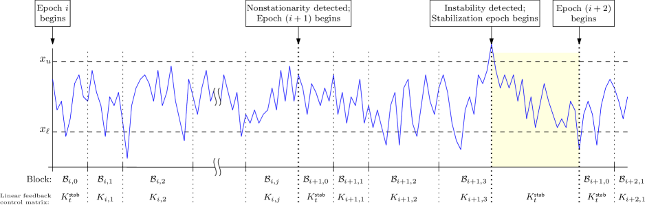
Figure 1: Illustration of Regular epochs, blocks, and stabilization epochs for Algorithm Dyn-LQR. Epoch $i$ ends in block $\mathcal{B}_{i,j}$ when an EndOfExplorationTest fails. Epoch $i+1$ ends because $\left\lVert x_{t}\right\rVert$ exceeds the threshold $x_{u}$, indicating that the current controller $K_{i+1,3}$ is potentially unstable. This triggers a stabilization epoch which ends the first time $\left\lVert x_{t}\right\rVert$ falls below $x_{\ell}$, and starts epoch $i+2$.

Our algorithm Dyn-LQR is presented as Algorithm 1. At a high level, the algorithm divides the time horizon into epochs $\{\mathcal{E}_{1},\mathcal{E}_{2},\ldots\}$ where the squared total variation $\Delta^{2}_{\mathcal{E}_{i}}$ within epoch $\mathcal{E}_{i}$ is of the order $\sqrt{1/|\mathcal{E}_{i}|}$. This should be reminiscent of the trade-off described in the last paragraph of Section 3 where the variance of the OLS estimator for a block was proportional to the inverse square root of the length of the block. The end of an epoch signals that a sufficient change in $\Theta_{t}$ has accumulated and the algorithm starts a new epoch, whereby it forgets the past history and restarts the procedure to estimate the dynamics $\Theta_{t}$. Since the length of an epoch is unknown to the online controller a priori, within each epoch we follow a doubling strategy (again similar to the naive algorithm in Section 3) by further splitting it into non-overlapping blocks (indexed by $j=0,1,\ldots$) of geometrically increasing duration. We denote the $j$-th block of epoch $i$ as $\mathcal{B}_{i,j}$. During block 0, or the warm-up block, the algorithm plays an action $u_{t}=K^{\textsf{stab}}_{t}x_{t}+\nu_{0}\eta_{t}$ where $\eta_{t}\sim\mathcal{N}(0,I_{d})$ are i.i.d. Gaussian random vectors, and $\nu_{0}=1$ is the added exploration noise. We denote by $\{\mathcal{G}_{t}\}_{t\in[T]}$ the filtration generated by $\{\eta_{1},\ldots,\eta_{T}\}$. The duration of the warm-up blocks is $L=\mathcal{O}((n+d)\log^{3}T)$. The $\mathcal{O}(1)$ exploration noise reduces the estimation error of the OLS estimate computed at the end of the block. Observations from block $j$ are used to create an estimate $\widehat{\Theta}_{i,j}$ of the dynamics, which in turn gives the linear feedback controller for block $j+1$ as $K_{i,j+1}:=K^{*}(\widehat{\Theta}_{i,j})$, and action $u_{t}=K_{i,j+1}x_{t}+\nu_{j+1}\eta_{t}$. For a block $\mathcal{B}_{i,j}$ with $j\geq 1$, we choose $\nu^{2}_{j}\approx\frac{1}{\sqrt{|\mathcal{B}_{i,j}|}}$ as the exploration noise similar to the stationary LQR case. If the estimate based on a block $\mathcal{B}_{i,j}$ “differs statistically” from the estimate from the previous block $\mathcal{B}_{i,j-1}$ (Algorithm 3), epoch $\mathcal{E}_{i}$ is ended and $\mathcal{E}_{i+1}$ started. Figure 1 gives an illustration of epochs and blocks.

Algorithm 1 Dyn-LQR

Input:

Horizon $T$, stabilizing controllers $\{K^{\textsf{stab}}_{t}\}$, input instance parameters $\rho_{0},\psi,\kappa,\beta$

1 Definition: $\nu_{0}=1$; $\nu_{j}^{2}=\sqrt{\frac{C_{0}}{2^{j}L}}$ for $j\geq 1$ where $C_{0}=4\log T$, $L=\frac{16(n+d)\log^{3}T}{1-\rho_{0}}$;

2       $\mathcal{B}_{i,j}=[\tau_{i}+2^{j-1}L,\tau_{i}+2^{j}L-1]$, where $\tau_{i}$ is the start of exploration epoch $\mathcal{E}_{i}$;

3       Bounds on $\left\lVert x_{t}\right\rVert$ for stabilization epochs: $x_{u}=2\kappa e^{C_{ss}}\left(\frac{\sqrt{8(n+d)}\beta}{\sqrt{1-\rho_{0}}}\sqrt{\log T}+\frac{(n+d)B}{1-\rho_{0}}\right),x_{\ell}=\frac{2\psi\kappa\sqrt{n}}{1-\rho_{0}}$;

4       $\eta_{t}\stackrel{{\scriptstyle i.i.d.}}{{\sim}}\mathcal{N}(0,I_{n})$;

5 Initialize: $t=1,i=1$;

$\tau_{i}\leftarrow t$ ;

  /* Start of exploration epoch $\mathcal{E}_{i}$ */

6 for $t=\tau_{i},\ldots,\tau_{i}+L-1$ do /* Block $0$ (warm-up) */

7       Play $u_{t}=K^{\textsf{stab}}_{t}x_{t}+\nu_{0}\eta_{t}$;

8      

9 end for

10for $j=1,2,\dots$ do

11       Let $\widehat{\Theta}_{i,j-1}$ be the OLS estimator based on $\mathcal{B}_{i,j-1}$, and define $K_{i,j}=K^{*}(\widehat{\Theta}_{i,j-1})$;

       $\mathcal{M}\leftarrow\emptyset$ ;

        /* Initialize the set of exploration phases */

12       while $t\leq\tau_{i}+2^{j}L-1$ do

             $E\sim\textsf{Ber}\left(\frac{1}{L}2^{-j/2}\sum_{m=0}^{j-1}2^{-m/2}\right)$ ;

              /* Sample exploration indicator */

13             if $E=1$ then

14                   Sample exploration scale index $m\in\{0,1,2,\dots,j-1\}$ with probability $\text{Pr}(m=b)\propto 2^{-b/2}$;

15                   $\mathcal{M}\leftarrow\mathcal{M}\cup\{(m,t)\}$;

16                  

17             end if

            Let $M_{t}=\{(m,s)\in\mathcal{M}\ |\ s\leq t\leq s+2^{m}L-1\}$ ;

              /* Active exploration phases */

18             if $M_{t}\neq\emptyset$ then

19                   Set $m_{t}=\min\{m\ |\ \exists(m,s)\in M_{t}\}$;

20                   Play $u_{t}=K_{i,j}x_{t}+\nu_{m_{t}}\eta_{t}$;

21                  

22            else

23                   Play $u_{t}=K_{i,j}x_{t}+\nu_{j}\eta_{t}$;

24                  

25             end if

26            Observe $x_{t+1}$;

27             for $(m,s)\in\mathcal{M}\text{ with }t=s+2^{m}L-1$ do

28                   if $\textsc{EndOfExplorationTest}(i,j,m,s)=\textit{Fail}$ then

                         $t\leftarrow t+1$, $i\leftarrow i+1$ ; Go to line 1 ;

                          /* Start a new epoch */

29                        

30                   end if

31                  

32             end for

33            if $t=\tau_{i}+2^{j}L-1$ and $\textsc{EndOfBlockTest}(i,j)=\textit{Fail}$  then

                   $t\leftarrow t+1$, $i\leftarrow i+1$ ; Go to line 1 ;

                    /* Start a new epoch */

34                  

35             end if

36            $t\leftarrow t+1$;

37             if $\left\lVert x_{t}\right\rVert\geq x_{u}$ then /* Instability detected */

38                   while $\left\lVert x_{t}\right\rVert\geq x_{\ell}$ do

39                         Play $u_{t}=K^{\textsf{stab}}_{t}x_{t}$, observe $x_{t+1}$;

40                         $t\leftarrow t+1$;

41                        

42                   end while

                  $i\leftarrow i+1$ ; Go to line 1 ;

                    /* Start a new epoch */

43                  

44             end if

45            

46       end while

47      

48 end for

Construct OLS estimator $\widehat{\Theta}_{i,j,(m,s)}$;

$\widehat{\Theta}_{i,j,(m,s)}=\mathop{\mathrm{argmin}}_{\Theta}\sum_{t=s}^{s+2^{m}L-1}\left\lVert x_{t+1}-\Theta[x_{t}^{\top}u_{t}^{\top}]^{\top}\right\rVert_{F}^{2}$;

if $\left\lVert\widehat{\Theta}_{i,j-1}-\widehat{\Theta}_{i,j,(m,s)}\right\rVert_{F}^{2}\geq(1+\bar{C}_{\textsf{bias}}+2\bar{C}_{\textsf{var}})^{2}(2^{m}L)^{-1/2}$ then /* See (7) */

       Return Fail;

      

end if

Return Pass;

Algorithm 2 EndOfExplorationTest($i,j,m,s$)

Construct OLS estimator $\widehat{\Theta}_{i,j}$ ;

$\widehat{\Theta}_{i,j}=\mathop{\mathrm{argmin}}_{\Theta}\sum_{t\in\mathcal{B}_{i,j}}\left\lVert x_{t+1}-\Theta[x_{t}^{\top}u_{t}^{\top}]^{\top}\right\rVert_{F}^{2}$;

if $\left\lVert\widehat{\Theta}_{i,j-1}-\widehat{\Theta}_{i,j}\right\rVert_{F}^{2}\geq(1+\bar{C}_{\textsf{bias}}+2\bar{C}_{\textsf{var}})^{2}(2^{j-1}L)^{-1/2}$ then /* See (7) */

       Return Fail;

      

else

       Return Pass;

      

end if

Algorithm 3 EndOfBlockTest($i,j$)

The vanilla policy mentioned above suffers from the problem that we could potentially commit to a controller for a long block – and hence fail to detect a large change, which could in turn potentially lead to $\mathcal{O}(T)$ regret. This is where the crucial novelty of the scheme of Chen et al. (2019) (designed for contextual multi-armed bandits) comes into play: to detect non-stationarity, which may happen at different scales (few large or many small changes), at each time within the block $\mathcal{B}_{i,j}$, the authors’ algorithm enters a replay phase where the policy from an earlier block in the same epoch (together with the larger exploration noise) is played. If at the end of some replay phase, the estimate of reward differs significantly from the history, the current epoch is ended. The algorithm could potentially be in multiple replay phases simultaneously, in which case the policy to replay is picked uniformly at random from active replays. Replay phases with different indexes are intended to detect changes of different magnitudes.

To adapt to the LQR setting, we simplify the above strategy. In particular, at any time $t$ in a block $\mathcal{B}_{i,j}$, we enter an exploration phase with probability proportional to $1/\sqrt{|\mathcal{B}_{i,j}|}$ and given this event happens, the ‘scale’ of the exploration phase is chosen to be $m$ with probability proportional to $1/\sqrt{2^{m}}$. A scale $m$ exploration phase lasts for $2^{m}L$ time steps, during which we play the action $u_{t}=K_{i,j}x_{t}+\sigma_{t}\eta_{t}$. That is, we keep playing the same linear feedback controller, but with exploration noise increased to $\sigma^{2}_{t}\approx\frac{1}{\sqrt{2^{m}}}$. Therefore, a scale $m$ exploration phase allows us to detect variation in $\Theta_{t}$ of size $\sqrt[4]{1/2^{m}}$. There can be multiple exploration phases active at any time $t$. We denote them by $M_{t}=\{(m_{1},t_{1}),(m_{2},t_{2}),\ldots\}$ where $m_{k}$ denotes the scale and $t_{k}$ denotes the starting time of the $k$-th active exploration phase. In this case, we play the most aggressive (i.e., the smallest $m$) exploration phase, with the feedback used by all active exploration phases to improve their estimates. At the end of the exploration phase $(m,s)$, we first compute the OLS estimator $\Theta_{i,j,(m,s)}$, and declare non-stationarity and end the epoch if $\left\lVert\widehat{\Theta}_{i,j-1}-\widehat{\Theta}_{i,j,(m,s)}\right\rVert^{2}\gtrapprox\frac{1}{\sqrt{2^{m}}}$ (Algorithm 2).

One crucial difference between LQR and the contextual bandit setting off Chen et al. (2019) is that LQR has a quadratic cost, while contextual bandit is a special case of a linear bandit problem, which affects the choice of $\sigma_{t}$. Yet another crucial difference from the contextual bandit setting is that since the LQR system has a state, the system could potentially become unstable through an inaccurate estimate before the non-stationarity is detected. We thus create a third criterion for ending an epoch: whenever $\left\lVert x_{t}\right\rVert\geq x_{u}=\mathcal{O}\left(\frac{\sqrt{(n+d)\log T}}{1-\rho_{0}}\right)$, we end the current epoch and enter a stabilization epoch. In a stabilization epoch we keep playing the stabilizing controllers without any exploration noise until $\left\lVert x_{t}\right\rVert$ drops below $x_{\ell}=\mathcal{O}\left(\frac{n}{1-\rho_{0}}\right)$. At this point, we begin a regular exploration epoch.

6 Estimation error for OLS with non-stationary $\Theta_{t}$

A central ingredient of our algorithm is the ordinary least squares estimator used to learn the approximate dynamics. While the study of the variance of the OLS estimator is a well-understood topic, when the parameter sequence is non-stationary, the OLS estimator can be biased. Studying this bias is quite non-trivial, especially for the LQR problem.

We state our results on the estimation error of the OLS estimator for non-stationary LQR at the end of this section and devote Appendix C to the formal proofs of the results. However, we will highlight in brief the reason that these results are challenging and non-trivial. For intuition, the reader should keep the trade-off we pointed to at the end of Section 3 in mind: during an interval ${\mathcal{I}}$ of length $|{\mathcal{I}}|$, to balance the exploration-exploitation trade-off we would like to create an estimator that has error of order $|{\mathcal{I}}|^{-1/4}$. With a non-stationary parameter sequence, this error comes from both the variance of the estimator as well as the bias. Therefore, if the variation in $\Theta_{t}$ during this interval, $\Delta_{{\mathcal{I}}}$, is of smaller order than $|{\mathcal{I}}|^{-1/4}$, then we would like the bias of our estimator to be $\mathcal{O}(\Delta_{{\mathcal{I}}})$.

Failure of a naive proof-strategy.

We first show that an obvious first line of attack to bound the estimation error of OLS does not work. Define $z_{t}=[x_{t}^{\top},u_{t}^{\top}]^{\top}$ and $\Upsilon_{\mathcal{I}}\coloneqq\sum_{t\in{\mathcal{I}}}z_{t}z_{t}^{\top}$ for an interval ${\mathcal{I}}=[s,e]$. Then we can write the error in the OLS estimator compared to a ‘representative’ $\bar{\Theta}$ (e.g., $\bar{\Theta}=\Theta_{e}$) as:

$$\widehat{\Theta}_{{\mathcal{I}}}-\bar{\Theta}=\underbrace{\left(\sum_{t\in{\mathcal{I}}}\left(\Theta_{t}-\bar{\Theta}\right)z_{t}z_{t}^{\top}\right)\Upsilon_{{\mathcal{I}}}^{-1}}_{\footnotesize\mbox{``bias''}}+\underbrace{\left(\sum_{t\in{\mathcal{I}}}w_{t}z_{t}^{\top}\right)\Upsilon_{{\mathcal{I}}}^{-1}}_{\footnotesize\mbox{``variance''}}.$$

The above shows that if $\Theta_{t}$ is constant in ${\mathcal{I}}$, then the estimator is unbiased. Lacking that, we may try to bound the first term as follows (this proof strategy was followed in Cheung et al. (2019a)). Let $\bar{\Theta}=\Theta_{e}$, then

$$\left\lVert\left(\sum_{t\in{\mathcal{I}}}\left(\Theta_{t}-\Theta_{e}\right)z_{t}z_{t}^{\top}\right)\Upsilon_{{\mathcal{I}}}^{-1}\right\rVert_{F}=\left\lVert\left(\sum_{t\in{\mathcal{I}}}\sum_{p=t}^{e-1}\left(\Theta_{p}-\Theta_{p+1}\right)z_{t}z_{t}^{\top}\right)\Upsilon_{{\mathcal{I}}}^{-1}\right\rVert_{F}$$

$$\qquad\qquad=\ \left\lVert\sum_{p=s}^{e-1}\left(\Theta_{p}-\Theta_{p+1}\right)\left(\sum_{t=s}^{p-1}z_{s}z_{s}^{\top}\right)\Upsilon_{{\mathcal{I}}}^{-1}\right\rVert_{F}\ \leq\ \sum_{p=s}^{e-1}\left\lVert\left(\Theta_{p}-\Theta_{p+1}\right)\right\rVert_{F}\lambda_{\max}\left(\left(\sum_{t=s}^{p-1}z_{s}z_{s}^{\top}\right)\Upsilon_{{\mathcal{I}}}^{-1}\right).$$

If $\lambda_{\max}\left(\left(\sum_{t=s}^{p-1}z_{s}z_{s}^{\top}\right)\Upsilon_{{\mathcal{I}}}^{-1}\right)\leq 1$, then the analysis above would bound the bias by $\Delta_{{\mathcal{I}}}$. While this may seem intuitive (e.g., it is true if $z_{s}$ are scalars), this was shown to be false for an arbitrary $\{z_{s}\}$ sequence even for the case of $z_{s}\in\mathbb{R}^{2}$ by Zhao and Zhang (2021).

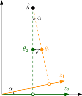
Figure 2: Illustration for the large bias of OLS estimator with non-stationary parameters.

An illustrative example.

To further highlight why a technically challenging analysis is necessary for the study of OLS with a non-stationary parameter sequence, we consider a simple example of OLS estimation without noise. Consider a 2-dimensional example with two data points:

$$\theta_{1}\ =\ [1\ \ 1],\quad\theta_{2}\ =\ [1-\epsilon\ \ 1];\qquad z_{1}\ =\ [\cos\alpha\ \ \sin\alpha],\quad z_{2}\ =\ [1\ \ 0].$$

Figure 2 shows the geometric intuition behind the OLS estimator. In this specific example, the estimate is given by the intersection of two (for $t=1,2$) lines: perpendicular to $z_{t}$ and passing through $\theta_{t}$. The bias of the OLS estimate $\widehat{\theta}$ in this noiseless case is given as $|\widehat{\theta}-\theta_{2}|=\epsilon/\tan\alpha$. With $\alpha\approx\epsilon\ll 1$, the bias approaches $1$ even though $\theta_{1},\theta_{2}$ are $\epsilon$-close to each other. The matrix $\Upsilon$ for this case is

$$\Upsilon=\begin{bmatrix}1+\cos^{2}\alpha&\cos\alpha\cdot\sin\alpha\\ \cos\alpha\cdot\sin\alpha&\sin^{2}\alpha\end{bmatrix},$$

which is ill-conditioned when $\alpha\ll 1$. In particular, $\lambda_{\max}(\Upsilon)/\lambda_{\min}(\Upsilon)\approx 1/2\alpha^{2}$. It might seem that such an ill-conditioned $\Upsilon$ is an extreme case that is unlikely to bother our study. However, with the exploration noise chosen in Algorithm 1, we give evidence in Lemma 40 that the condition number of $\Upsilon_{{\mathcal{I}}}$ for intervals ${\mathcal{I}}$ of interest is concentrated around $\mathcal{O}(\sqrt{|{\mathcal{I}}|})$, while we are trying to get unbiased estimates when the variation of $\Theta_{t}$ in interval ${\mathcal{I}}$ is $\Delta_{{\mathcal{I}}}=\mathcal{O}(|{\mathcal{I}}|^{-1/4})$. This precisely corresponds to the problematic setting $\alpha\sim\epsilon\ll 1$ in our toy example above.

Our proof approach.

We begin by decomposing the problem into bounding the estimation error for each row of the estimate $\widehat{\Theta}_{{\mathcal{I}}}$. For a given row, $\widehat{\theta}_{{\mathcal{I}}}$, the key obstacle in the analysis of the estimation error $\left\lVert\widehat{\theta}_{{\mathcal{I}}}-\bar{\theta}\right\rVert^{2}$ is that while $z_{t}$ lives in $\mathbb{R}^{n+d}$, most of its variance is in the $n$-dimensional column space of $[I_{n}\ K_{\mathcal{I}}^{\top}]^{\top}$, where $K_{\mathcal{I}}$ is the fixed linear feedback controller used during interval ${\mathcal{I}}$. This is because the LQR dynamics naturally adds the noise $w_{t-1}$ to arrive at the state $x_{t}$ allowing efficient exploration/estimation of the component of $\bar{\theta}$ lying in the column space of $[I_{n}\ K_{\mathcal{I}}^{\top}]^{\top}$. In particular, the total energy in this column space is $\mathcal{O}(|{\mathcal{I}}|)$ through $w_{t}$, while the energy in the orthogonal subspace through the exploration noise $\xi_{t}=\sigma_{t}\eta_{t}$ is $\sum_{t\in{\mathcal{I}}}\sigma^{2}_{t}=\mathcal{O}(\sqrt{|{\mathcal{I}}|})$. Therefore, as our toy example points out, a naive analysis based on a lower bound on the eigenvalues of the matrix $\sum_{t\in{\mathcal{I}}}z_{t}z_{t}^{\top}$ fails, because it does not exploit the statistical independence between $\xi_{t}$ and $x_{t}$.

Our approach is to instead to look at one-dimensional OLS problems parameterized by directions $v\in\mathbb{S}^{n+d}:=\{v\in\mathbb{R}^{n+d},\left\lVert v\right\rVert=1\}$:

$$\lambda_{v}=\mathop{\mathrm{argmin}}_{\lambda}\mathcal{L}(\bar{\theta}+\lambda\cdot v),$$

where $\mathcal{L}$ is the quadratic loss function for OLS. We argue that $|\lambda_{v}|$ are small for ‘enough’ directions $v$. That is, in enough directions, the minimizer $\left(\bar{\theta}+\lambda_{v}\cdot v\right)$ of the 1-dimensional quadratic defined above is close to the candidate $\bar{\theta}$. Furthermore, since the loss function looks very different for $v$ lying close to the column space of $[I_{n}\ K^{\top}]^{\top}$ versus $v$ lying close to its orthogonal subspace, we consider two cases: $v$ lying only in the column space or lying only in its orthogonal subspace, and prove that the geometry of Hessian implies that it is sufficient to look at these two cases. The complete proof is presented in Appendix C.

Results

We state our lemmas for the estimation error for the OLS estimators used in Algorithm 1. Lemma 8 states it for intervals within exploration blocks $\mathcal{B}_{i,j}$, while Lemma 9 states it for warm-up blocks $\mathcal{B}_{i,0}$. The reason for the two separate results is that within a warm-up block, the controller $K_{t}^{\textsf{stab}}$ is changing, which does not allow a subspace decomposition we mentioned earlier, but the $\mathcal{O}(1)$ exploration noise still allows us to bound the estimation error. Within an exploration block $\mathcal{B}_{i,j}$, the exploration noise is of a much smaller magnitude (to control regret due to exploration), but the controller $K_{t}$ is fixed, which allows the decomposition.

Lemma 8.

Consider an interval ${\mathcal{I}}$ in block $\mathcal{B}_{i,j}$ for some epoch $\mathcal{E}_{i}$ in Algorithm 1, such that $|{\mathcal{I}}|\geq L$ and $\max_{t\in{\mathcal{I}}}\left\lVert x_{t}\right\rVert\leq x_{u}$. Let $\widehat{\Theta}_{{\mathcal{I}}}$ be the corresponding OLS estimate from observations in ${\mathcal{I}}$ and $\bar{\Theta}=\Theta_{t}$ for some $t\in{\mathcal{I}}$. Then, there exists a $T_{0}$, such that for $T\geq T_{0}$, with probability at least $1-\varepsilon$:

$$\left\lVert\widehat{\Theta}_{{\mathcal{I}}}-\bar{\Theta}\right\rVert_{F} \leq\breve{C}_{1}\Delta_{\mathcal{I}}+\breve{C}_{2}|{\mathcal{I}}|^{-\frac{1}{4}},$$

where

$$\breve{C}_{1}=C_{\textsf{bias}}\sqrt{\ln\frac{1}{\varepsilon}+\ln T}\quad\mbox{and}\qquad\breve{C}_{2}=C_{\textsf{var}}\left(\sqrt{\ln T}+\sqrt{\ln\frac{1}{\varepsilon}}\right),$$

for problem dependent constants $C_{\textsf{bias}},C_{\textsf{var}}$ (precise expressions are shown in (C.1)).

Lemma 9.

Consider a warm-up block $\mathcal{B}_{i,0}$ in Algorithm 1 and let $\bar{\Theta}=\Theta_{t}$ for some $t\in\mathcal{B}_{i,0}$. There exists a $T_{0}$, such that for $T\geq T_{0}$ and the choice of $L$ in Algorithm 1, the OLS estimate $\widehat{\Theta}_{\mathcal{B}_{i,0}}$ of a warm-up block $\mathcal{B}_{i,0}$ satisfies

$$\left\lVert\widehat{\Theta}_{\mathcal{B}_{i,0}}-\bar{\Theta}\right\rVert_{F} \leq\breve{C}_{1,\textsf{stab}}\Delta_{\mathcal{B}_{i,0}}+\breve{C}_{2,\textsf{stab}}|\mathcal{B}_{i,0}|^{-\frac{1}{4}},$$

with probability at least $1-\varepsilon$ where

$$\breve{C}_{1,\textsf{stab}}=C_{\textsf{bias},\textsf{stab}}\sqrt{\ln T}\quad\mbox{and}\qquad\breve{C}_{2,\textsf{stab}}=C_{\textsf{var},\textsf{stab}}\sqrt{\ln\frac{1}{\varepsilon}+\ln\ln T},$$

for problem dependent constants $C_{\textsf{bias},\textsf{stab}},C_{\textsf{var},\textsf{stab}}$ (precise expressions are shown in (C.2)).

Applying Lemma 8 and Lemma 9 with $\varepsilon=1/T^{3}$ to all the intervals (at most $T^{2}$) that may be considered during the execution of Algorithm 1 and a union bound immediately gives the following result.

Lemma 10.

Define Event 1 as the event that for each warm-up block $\mathcal{B}_{i,0}$ in Algorithm 1 it holds that

$$\left\lVert\widehat{\Theta}_{\mathcal{B}_{i,0}}-\bar{\Theta}\right\rVert_{F} \leq{C}_{\textsf{bias},\textsf{stab}}\sqrt{\ln T}\Delta_{\mathcal{B}_{i,0}}+3{C}_{\textsf{var},\textsf{stab}}\sqrt{\ln T}|\mathcal{B}_{i,0}|^{-\frac{1}{4}},$$

and for each phase and non-warmup block, denoted by ${\mathcal{I}}=[s,e]$, it holds that

$$\left\lVert\widehat{\Theta}_{{\mathcal{I}}}-\bar{\Theta}\right\rVert_{F}\leq 3C_{\textsf{bias}}\sqrt{\ln T}\Delta_{\mathcal{I}}+3C_{\textsf{var}}\sqrt{\ln T}|{\mathcal{I}}|^{-\frac{1}{4}}.$$

Then we have that $\text{{\bf Pr}$\left[\textsc{Event 1}\right]$}\geq 1-1/T$.

For succinctness, define

$$\bar{C}_{\textsf{bias}}=\sqrt{\ln T}\max\{3C_{\textsf{bias}},C_{\textsf{bias},\textsf{stab}}\}\quad\mbox{and}\quad\bar{C}_{\textsf{var}}=\sqrt{\ln T}\max\{3C_{\textsf{var}},3C_{\textsf{var},\textsf{stab}}\}.$$ (7)

7 Regret Upper Bound for Dyn-LQR

Our main regret upper bound for Dyn-LQR is shown below.

Theorem 11.

Under Assumption 3, the expected regret of Dyn-LQR is upper bounded as:

$$\text{{\bf E}$\left[\mathcal{R}^{\textsc{Dyn-LQR}}(T)\right]$}=\widetilde{\mathcal{O}}\left(V_{T}^{2/5}T^{3/5}\right).$$

If the dynamics $\{\Theta_{t}\}$ are piecewise constant with at most $S$ switches, then the regret of Dyn-LQR is upper bounded as:

$$\text{{\bf E}$\left[\mathcal{R}^{\textsc{Dyn-LQR}}(T)\right]$}=\widetilde{\mathcal{O}}\left(\sqrt{ST}\right).$$

Our definition of $\mathcal{R}^{\textsc{Dyn-LQR}}(T)$ in (1) measures the regret relative to the benchmark $\sum_{t=1}^{T}J^{*}_{t}$. In the next proposition, we prove that this benchmark is at most $\widetilde{\mathcal{O}}(V_{T})$ larger than the expected cost of the dynamic optimal policy. This additive error is dominated by the regret $\widetilde{\mathcal{O}}(V_{T}^{2/5}T^{3/5})$ proved in Theorem 11. Proposition 12 is proved in Appendix D.

Proposition 12.

Let $\{u_{t}\}_{t=1}^{T}$ be an arbitrary non-anticipative policy for the non-stationary LQR control problem. Then,

$$\text{{\bf E}$\left[\sum_{t=1}^{T}x_{t}^{\top}Qx_{t}+u_{t}^{\top}Ru_{t}\right]$}\geq\sum_{t=1}^{T}J^{*}_{t}-{\mathcal{O}}(V_{T}+\log T).$$

We will conduct our analysis under the assumption that Event 1 specified in Lemma 10 occurs. Since Dyn-LQR uses $K_{t}^{\textsf{stab}}$ whenever $\left\lVert x_{t}\right\rVert\geq x_{u}$, outside this event, the total cost is bounded by $\widetilde{\mathcal{O}}(T)$. Note that this happens with probability at most $1/T$.

7.1 Regret Decomposition

We begin with an informal regret decomposition lemma which highlights the key exploration-exploitation trade-off for non-stationary LQR.

Informal Lemma. The expected regret for a policy $\pi$ with $u_{t}=K_{t}x_{t}+\sigma_{t}\eta_{t}$ where $K_{t},\sigma_{t}$ are adapted to the filtration $(\mathcal{F},\mathcal{G})$ is given by:

E$$\left[\mathcal{R}^{\pi}(T)\right] =\text{{\bf E}$\left[\sum_{t=1}^{T}x_{t}^{\top}Qx_{t}+u_{t}^{\top}Ru_{t}-J^{*}_{t}\right]$}$$

$$= \ \underbrace{\sum_{t=1}^{T}\text{{\bf E}$\left[J_{t}(K_{t})-J^{*}_{t}\right]$}}_{\mbox{\footnotesize{exploitation regret}}}+\underbrace{\sum_{t=1}^{T}\text{{\bf E}$\left[\sigma_{t}^{2}\mathop{\mathrm{Tr}}\left(R+B_{t}^{\top}P_{t}(K_{t})B_{t}\right)\right]$}}_{\mbox{\footnotesize exploration regret}}$$

$$\quad+\underbrace{\sum_{t=1}^{T-1}\text{{\bf E}$\left[x_{t+1}^{\top}\left(P_{t+1}(K_{t+1})-P_{t}(K_{t})\right)x_{t+1}\right]$}}_{\mbox{\footnotesize policy/parameter variation}}+\text{{\bf E}$\left[x_{1}^{\top}P_{1}(K_{1})x_{1}-x_{T+1}^{\top}P_{T}(K_{T})x_{T+1}\right]$}.$$ (8)

We term the lemma informal because it relies on $J_{t}(K_{t})$ and $P_{t}(K_{t})$ being defined for all $t$. This need not always be true for Dyn-LQR since $K_{t}$ is the certainty equivalent controller based on an estimate of $\Theta_{t}$, and therefore the stationary system corresponding to $\Theta_{t}$ and $K_{t}$ need not even be stable, and $J_{t}(K_{t})$ could be unbounded. We shortly address how we handle such time periods, but their contribution to regret will be asymptotically of a smaller order. The decomposition points out that the dominant terms in the analysis will be the exploitation regret and the exploration regret. The policy/parameter variation depends on how much the pair $(\Theta_{t},K_{t})$ changes during non-warmup blocks of an exploration epoch. By design, the policies $\{K_{t}\}$ are piece-wise constant with at most $\log T$ changes per epoch, and we will prove that the number of epochs is $\mathcal{O}(V_{T}^{4/5}T^{1/5})$. Finally, for a fixed $K$, $\left\lVert P(\Theta_{t},K)-P(\Theta_{t+1},K)\right\rVert=\mathcal{O}(\left\lVert\Theta_{t}-\Theta_{t+1}\right\rVert)$, and hence this contributes at most $\mathcal{O}(V_{T})$ to the regret across the entire horizon.

To refine the regret decomposition, we recapitulate Algorithm 1, and in particular the classification of exploration epochs, stabilization epochs, blocks within exploration epochs, and another concept we define for the purpose of analysis alone – bad intervals.

(i) Stabilization epochs – such epochs begin whenever $\left\lVert x_{t}\right\rVert$ exceeds the upper bound $x_{u}$, indicating the potential instability of the current controller. We use $\tau^{\textsf{stab}}_{i}$ to denote the start of the $i$-th stabilization epoch. During a stabilization epoch, we use the controller $K_{t}=K^{\textsf{stab}}_{t}$. The $i$-th stabilization phase ends at $\theta_{i}^{\textsf{stab}}$ (inclusive) where

$$\theta^{\textsf{stab}}_{i}=\min\{t\geq\tau^{\textsf{stab}}_{i}+1\ :\ \left\lVert x_{t+1}\right\rVert\leq x_{\ell}\}.$$

We use ${\mathcal{S}}_{i}$ to denote the interval $[\tau^{\textsf{stab}}_{i},\theta^{\textsf{stab}}_{i}]$ as well as the $i$-th stabilization epoch symbolically.

(ii) Exploration epochs – such epochs begin either at the end of a stabilization epoch, or at the end of another exploration epoch if sufficient non-stationarity is detected through failure of EndOfExplorationTest or EndOfBlockTest. We will denote the start and end of the $i$-th exploration epoch by $\tau_{i}$ and $\theta_{i}$ respectively, and use $\mathcal{E}_{i}$ to denote the interval $[\tau_{i},\theta_{i}]$ as well as the epoch symbolically.

(iii) Blocks – The $i$-th exploration epoch $\mathcal{E}_{i}$ is partitioned into non-overlapping blocks of geometrically increasing duration. Block 0 (also called the warm-up block) is the interval $[\tau_{i},\tau_{i}+L-1]$, and the $j$-th block ($j=1,\ldots$) is the interval $[\tau_{i}+L\cdot 2^{j-1},\tau_{i}+L\cdot 2^{j}-1]\cap\mathcal{E}_{i}$ of maximum length $L\cdot 2^{j-1}$. We denote by $\mathcal{B}_{i,j}$ both the interval as well as the block symbolically. The controller used at time $t\in\mathcal{B}_{i,j}$ ($j\geq 1$) is given by $K^{*}(\widehat{\Theta}_{i,j-1})$, where $\widehat{\Theta}_{i,j-1}$ is the OLS estimator based on the block $j-1$ of epoch $\mathcal{E}_{i}$. For succinctness, we use the notation

$$\widehat{\Theta}_{t}:=\widehat{\Theta}_{i,j-1},\quad\mbox{for }t\in\mathcal{B}_{i,j}.$$

We will use $B_{i}$ to denote the number of blocks in epoch $\mathcal{E}_{i}$.

(iv) Bad/Good intervals – It can happen that for some time steps during an exploration epoch, the controller is unstable and therefore $J_{t}(K_{t})$ is undefined, but the $\left\lVert x_{t}\right\rVert$ has not exceeded $x_{u}$. To study the regret due to such $t$, we define the notion of bad intervals within epochs. The $k$-th bad interval of an epoch $i$ begins at $\tau_{i,k}^{\textsf{bad}}$ and ends at $\theta^{\textsf{bad}}_{i,k}$ where these are defined recursively as:

$$\tau^{\textsf{bad}}_{i,1} :=\min\left\{t\in[\tau_{i}+L,\theta_{i}]:\left\lVert\widehat{\Theta}_{t}-\Theta_{t}\right\rVert_{F}^{2}\geq C_{3}\right\},$$

$$\tau^{\textsf{bad}}_{i,k} :=\min\left\{t\in[\theta^{\textsf{bad}}_{i,k-1},\theta_{i}]:\left\lVert\widehat{\Theta}_{t}-\Theta_{t}\right\rVert_{F}^{2}\geq C_{3}\right\},$$

$$\theta^{\textsf{bad}}_{i,k} :=\min\left\{t\in[\tau^{\textsf{bad}}_{i,k}+1,\theta_{i}]\ :\ \left\lVert\widehat{\Theta}_{t+1}-\Theta_{t+1}\right\rVert_{F}^{2}\leq\frac{C_{3}}{2}\right\},$$

with the constant $C_{3}$ defined in Assumption 4. Note that we do not create bad intervals during the block $\mathcal{B}_{i,0}$, which is analyzed separately. We denote the $k$-th bad interval of an epoch $i$ as ${\mathcal{I}}^{\textsf{bad}}_{i,k}$. By ${\mathcal{I}}^{\textsf{bad}}_{i}$, we denote the union of all bad intervals in $\mathcal{E}_{i}$, and by ${\mathcal{I}}^{\textsf{bad}}$, the union of all bad intervals. All time periods that not in bad intervals, i.e., they are in $\mathcal{E}_{i}\setminus\{\mathcal{B}_{i,0}\cup{\mathcal{I}}^{\textsf{bad}}_{i}\}$, will be called good and split into good intervals. For analysis purposes, we further split the good time periods based on the blocks. That is, a good interval can end at time $t$ if (i) either a bad interval begins at time $t+1$, or (ii) a block ends at time $t$ in which case another good interval can begin at time $t+1$. Using a similar notation ${\mathcal{I}}^{\textsf{good}}_{i,j,k}$ denotes the $k$-th good interval of a block $\mathcal{B}_{i,j}$ (which must lie entirely inside $[\tau_{i}+L\cdot 2^{j-1},\tau_{i}+L\cdot 2^{j}-1]$. We will use $N^{\textsf{bad}}_{i}$ to denote the total number of bad intervals in an epoch $i$ and $N^{\textsf{good}}_{i,j}$ to denote the number of good intervals in a block $\mathcal{B}_{i,j}$. The advantage of defining the good intervals to lie within a block is that for the purposes of analysis, the good intervals within a block $\mathcal{B}_{i,j}$ are completely defined based on history before the start of the block $\mathcal{B}_{i,j}$.

We will use $E$ to denote the total number of exploration epochs and $E_{S}$ to denote the total number of stabilization epochs. Finally, we come to the regret decomposition that we use in the subsequent section:

$$\mathcal{R}^{\textsc{Dyn-LQR}}(T) =\sum_{t=1}^{T}c_{t}-J^{*}_{t}$$

$$\leq\underbrace{\sum_{i=1}^{E_{S}}\sum_{t\in{\mathcal{S}}_{i}}c_{t}}_{\begin{subarray}{c}\text{$T_{1}$: Stabilization}\\ \text{epochs}\end{subarray}}+\underbrace{\sum_{i=1}^{E}\sum_{t\in\mathcal{B}_{i,0}}c_{t}}_{\begin{subarray}{c}\text{$T_{2}$: Warm-up}\\ \text{blocks}\end{subarray}}+\underbrace{\sum_{i=1}^{E}\sum_{k=1}^{N^{\textsf{bad}}_{i}}\sum_{t\in{\mathcal{I}}^{\textsf{bad}}_{i,k}}c_{t}}_{\begin{subarray}{c}\text{$T_{3}$: Bad}\\ \text{intervals}\end{subarray}}+\underbrace{\sum_{i=1}^{E}\sum_{j=1}^{B_{i}}\sum_{k=1}^{N^{\textsf{good}}_{i,j}}\sum_{t\in{\mathcal{I}}^{\textsf{good}}_{i,j,k}}\left(c_{t}-J_{t}^{*}\right)}_{\begin{subarray}{c}\text{$T_{4}$: Good}\\ \text{intervals}\end{subarray}}.$$ (9)

7.2 Regret analysis for Dyn-LQR

The main result of this section is the following lemma, which provides an intermediate characterization of E$\left[\mathcal{R}^{\textsc{Dyn-LQR}}(T)\right]$ based on (9). In particular, the characterization highlights that to bound the regret, it is sufficient to bound (i) the number $E$ of exploration epochs (Section 7.3) and (ii) the total squared norm of the estimation error of dynamics $\Theta_{t}$ for the good periods (Section 7.4).

Lemma 13.

The expected regret for Dyn-LQR is bounded as follows:

E$$\left[\mathcal{R}^{\textsc{Dyn-LQR}}(T)\right] \leq\widetilde{\mathcal{O}}\left(\text{{\bf E}$\left[\sum_{i=1}^{E}\sum_{j=1}^{B_{i}}\sum_{t\in\mathcal{B}_{i,j}}\min\left\{\left\lVert\widehat{\Theta}_{i,j-1}-\Theta_{t}\right\rVert_{F}^{2},C_{3}\right\}+\sqrt{|\mathcal{B}_{i,j}|}\right]$}\right)+\widetilde{\mathcal{O}}(E+V_{T}),$$

$$\leq\widetilde{\mathcal{O}}\left(\text{{\bf E}$\left[\sum_{i=1}^{E}\sum_{j=1}^{B_{i}}\sum_{t\in\mathcal{B}_{i,j}}\min\left\{\left\lVert\widehat{\Theta}_{i,j-1}-\Theta_{t}\right\rVert_{F}^{2},C_{3}\right\}\right]$}\right)+\widetilde{\mathcal{O}}(\sqrt{E\cdot T}+V_{T}).$$ (10)

Proof.

We proceed by bounding the terms in (9).
Upper bound for Term 1. Since the controllers $\{K^{\textsf{stab}}_{t}\}$ used in a stabilization epoch satisfy sequentially strong stability (Assumption 3), in Lemma 14 we prove that the expected total cost per stabilization epoch is $\widetilde{\mathcal{O}}(1)$. Since the number of stabilization epochs is bounded by the number of exploration epochs $E$, the total contribution of Term 1 in (9) is $\widetilde{\mathcal{O}}(E)$.

Lemma 14.

Let $[\tau^{\textsf{stab}},\theta^{\textsf{stab}}]$ be a stabilization epoch. The expected total cost during the stabilization epoch is bounded by

$$\text{{\bf E}$\left[\left.\sum_{t=\tau^{\textsf{stab}}}^{\theta^{\textsf{stab}}}c_{t}\right|\mathcal{F}_{\tau^{\textsf{stab}}-1},\mathcal{G}_{\tau^{\textsf{stab}}-1}\right]$}=\mathcal{O}\left(\frac{\kappa^{2}x_{u}^{2}}{1-\rho_{0}}\right)={\mathcal{O}}\left(\frac{\kappa^{2}\beta^{2}(n+d+\log T)}{(1-\rho_{0})^{2}}\right).$$

Upper bound for Term 2. Similar to Lemma 14, the use of $K^{\textsf{stab}}_{t}$ during warm-up blocks gives a bound of $\widetilde{\mathcal{O}}(1)$ per epoch in Lemma 15, which gives a $\widetilde{\mathcal{O}}(E)$ contribution due to Term 2.

Lemma 15.

Let $[\tau_{i},\tau_{i}+L-1]$ denote the warm-up block $\mathcal{B}_{i,0}$ of an exploration epoch $\mathcal{E}_{i}$. The expected total cost during $\mathcal{B}_{i,0}$, for any $i$, is bounded by

$$\text{{\bf E}$\left[\left.\sum_{t=\tau_{i}}^{\tau_{i}+L-1}c_{t}\right|\mathcal{F}_{\tau_{i}-1},\mathcal{G}_{\tau_{i}-1}\right]$}={\mathcal{O}}\left(\frac{\kappa^{2}\beta^{2}(n+d)\log^{3}T}{(1-\rho_{0})^{2}}\right).$$

Upper bound for Term 3. Since $\left\lVert x_{t}\right\rVert$ is bounded by $x_{u}=\widetilde{\mathcal{O}}(1)$ for any time period in a bad interval by definition, the cost is bounded by $\widetilde{\mathcal{O}}(1)$ per time step. We can bound the number of bad time periods within an arbitrary interval ${\mathcal{I}}$ noting that for $t\in{\mathcal{I}}^{\textsf{bad}}$, $\left\lVert\widehat{\Theta}_{t}-\Theta_{t}\right\rVert_{F}^{2}\geq C_{3}/2$ and thus:

$$\left|{\mathcal{I}}^{\textsf{bad}}\cap{\mathcal{I}}\right| =\sum_{t\in{\mathcal{I}}^{\textsf{bad}}\cap{\mathcal{I}}}1\leq\frac{2}{C_{3}}\sum_{t\in{\mathcal{I}}}\min\left\{\left\lVert\widehat{\Theta}_{t}-{\Theta}_{t}\right\rVert_{F}^{2},C_{3}\right\}.$$ (11)

Then the total contribution of Term 3 is ${\mathcal{O}}\left(\text{{\bf E}$\left[\sum_{i=1}^{E}\sum_{j=1}^{B_{i}}\sum_{t\in\mathcal{B}_{i,j}}\min\left\{\left\lVert\widehat{\Theta}_{i,j-1}-\Theta_{t}\right\rVert_{F}^{2},C_{3}\right\}\right]$}\right)$.

Upper bound for Term 4.

Lemma 16.

For some epoch $\mathcal{E}_{i}$, a block $\mathcal{B}_{i,j}$ in epoch $\mathcal{E}_{i}$, and a good interval ${\mathcal{I}}^{\textsf{good}}_{i,j,k}=[\tau,\theta]$ in block $\mathcal{B}_{i,j}$, the expected regret is bounded as follows:

E$$\left[\mathcal{R}^{\pi}({\mathcal{I}}^{\textsf{good}}_{i,j,k})\mid\mathcal{F}_{\tau-1},\mathcal{G}_{\tau-1}\right]$$

$$\qquad\leq\sum_{t=\tau}^{\theta}\left(J_{t}(K_{t})-J^{*}_{t}\right)+\left|{\mathcal{I}}^{\textsf{good}}_{i,j,k}\right|\frac{C_{0}^{1/2}}{L^{3/2}}\cdot\frac{j}{\sqrt{2^{j}}}+{\mathcal{O}}\left(\frac{n+d+\log T}{1-\rho_{0}}\left(1+\Delta_{{\mathcal{I}}_{i,j,k}}\right)\right)$$

$$\qquad\leq\sum_{t=\tau}^{\theta}C_{4}\left\lVert\widehat{\Theta}_{i,j-1}-\Theta_{t}\right\rVert_{F}^{2}+\left|{\mathcal{I}}^{\textsf{good}}_{i,j,k}\right|\frac{C_{0}^{1/2}C_{7}}{L^{3/2}}\cdot\frac{j}{\sqrt{2^{j}}}+{\mathcal{O}}\left(\frac{n+d+\log T}{1-\rho_{0}}\left(1+\Delta_{{\mathcal{I}}_{i,j,k}}\right)\right),$$

where the constant $C_{7}:=\max_{t}\sup\left\{\mathop{\mathrm{Tr}}\left(R+B_{t}^{\top}P_{t}(K_{t})B_{t}\right)\mid K_{t}=K^{*}(\widehat{\Theta}),\left\lVert\widehat{\Theta}-\Theta_{t}\right\rVert_{F}^{2}\leq C_{3}\right\}$.

Combining the results above, we can bound the first term in (13) immediately from Term 3 and the first summand in Lemma 16 for Term 4. Summing the second term in Lemma 16 over all the good intervals within a block $\mathcal{B}_{i,j}$ (which is of length at most $2^{j}$) contributes $\widetilde{\mathcal{O}}(\sqrt{|\mathcal{B}_{i,j}|})$. Since the blocks within an epoch are doubling in length, $\sum_{j}\sqrt{|\mathcal{B}_{i,j}|}\leq 8\sqrt{|\mathcal{E}_{i}|}$ and $\sum_{i}\sqrt{|\mathcal{E}_{i}|}\leq E\sqrt{T/E}=\sqrt{E\cdot T}$. The contribution of the third term in Lemma 16 is proportional to the number of good intervals, which is bounded by $V_{t}/\sqrt{C_{3}/2}+E\log T$. To see this, note that without any bad intervals, there would be one good interval per block and there are at most $\log T$ blocks per epoch. For a good interval to begin due to a bad interval ending, the bad interval must ‘eat up’ $\sqrt{C_{3}/2}$ of the variation due to the criterion chosen for the end of a bad interval. Hence, there can be at most $V_{T}/\sqrt{C_{3}/2}$ good intervals created because of the bad intervals. The last term in Lemma 16 contributes $\widetilde{\mathcal{O}}(V_{T})$ to (13). ∎

7.3 Bounding the Number of Epochs

There are two ways of generating epochs in Algorithm 1: (1) epochs end due to the detection of non-stationarity (lines 1 and 1), and (2) epochs end due to the detection of instability (line 1). This section is devoted to bounding the number of epochs from these two sources separately.

Bounding the number of epochs generated by non-stationarity tests.

In the subsequent analysis, we will bound the number of epochs terminated due to the detection of non-stationarity in $\Theta_{t}$ by $\mathcal{O}(T^{1/5}V_{T}^{4/5})$, which dominates $\mathcal{O}(V_{T})$. Recall that an epoch ends if the non-stationarity tests in Algorithms 2 or 3 fail, which happens if the distance between the new OLS estimate and the estimate based on the previous block exceeds some threshold. The thresholds there are carefully designed according to the concentration results proved in Section 6, which allow us to prove the following lemma characterizing the variation budget needed for an epoch to fail the tests in Algorithms 2 and 3.

Lemma 17.

Assume Event 1 holds. Let $\mathcal{E}_{i}$ be an epoch with total variation $\Delta_{[\tau_{i},t]}\leq(t-\tau_{i}+1)^{-1/4}$, then the epoch does not end because of nonstationarity detection.

The following corollary bounds the number of restarts due to detection of non-stationarity.

Corollary 18.

Assume Event 1 holds. The number of epochs that end due to detection of non-stationarity is bounded by $\mathcal{O}(C_{0}^{-2/5}T^{1/5}V_{T}^{4/5})$.

Bounding the number of epochs generated by instability tests.

Lemma 19 characterizes the variation budget needed to trigger the end of an epoch due to instability detection, which leads to Corollary 20 bounding the number of epochs ended due to instability.

Lemma 19.

Let $\mathcal{E}_{i}$ be an epoch with total variation $\Delta_{\mathcal{E}_{i}}\leq\left(\sqrt{\frac{C_{3}}{4}}-\bar{C}_{\textsf{var}}L^{-1/4}\right)/\bar{C}_{bias}$. Then under Event 1, with probability at least $1-\mathcal{O}(1/T^{3})$, the epoch does not end because of instability detection.

Corollary 20.

The expected number of epochs that end due to the instability test is bounded by $\mathcal{O}(V_{T}\sqrt{\ln T})$.

Combining the two bounds, we get $E=\mathcal{O}(T^{1/5}V_{T}^{4/5})$. Therefore, we can bound the $\widetilde{\mathcal{O}}(\sqrt{E\cdot T})$ term in (13) by $\widetilde{\mathcal{O}}(T^{3/5}V_{T}^{2/5})$.

7.4 Bounding the Total Square Norm of the Estimation Error

In this section, we analyse the regret due to the estimation error, i.e., the first term in (13). For succinctness, define the following loss function for an arbitrary interval ${\mathcal{I}}$:

$$\mathcal{L}(I) :=\sum_{t\in{\mathcal{I}}}\min\left\{C_{4}\left\lVert\widehat{\Theta}_{i,j-1}-\Theta_{t}\right\rVert_{F}^{2},C_{3}\right\}.$$ (12)

In the sequel, we first focus on an exploration epoch $\mathcal{E}_{i}$ and bound $\mathcal{L}(\mathcal{E}_{i})$. We then combine the regret of epochs to get the requisite regret bound of Theorem 11.

Our proof decomposes into three parts. First, we focus on one block, say block $j$, of epoch $i$, and prove a lemma that provides an upper bound for $\mathcal{L}({\mathcal{I}})$ for any interval ${\mathcal{I}}\subseteq\mathcal{B}_{i,j}$. Second, we partition a block into intervals with small total variation within each interval. We use the just mentioned bound to bound $\mathcal{L}(\mathcal{B}_{i,j})$ of each block $j$ in an exploration epoch $i$ in terms of the length of the block and the total variation within the block. Finally, we upper bound the total number of blocks within an epoch $i$ and sum up the bound on $\mathcal{L}(\mathcal{B}_{i,j})$ for all the blocks in an epoch $\mathcal{E}_{i}$ to obtain a bound on $\mathcal{L}(\mathcal{E}_{i})$.

Lemma 21.

For an arbitrary interval ${\mathcal{I}}=[s,e]$ that lies in block $\mathcal{B}_{i,j}$, define $\varepsilon_{\mathcal{I}}\coloneqq\left\lVert\widehat{\Theta}_{i,j-1}-\Theta_{s}\right\rVert_{F}^{2}$ and $\alpha_{\mathcal{I}}\coloneqq\frac{\log{|{\mathcal{I}}|}}{\sqrt{{\mathcal{I}}}}$. Then, $\mathcal{L}({\mathcal{I}})$ can be bounded as

$$\mathcal{L}({\mathcal{I}}) =\mathcal{O}\left(|{\mathcal{I}}|\alpha_{{\mathcal{I}}}+|{\mathcal{I}}|\Delta^{2}_{{\mathcal{I}}}+|{\mathcal{I}}|\varepsilon_{\mathcal{I}}\mathbbm{1}\{\varepsilon_{\mathcal{I}}\geq\alpha_{\mathcal{I}}\}\right).$$

To get a bound for the regret for a block, we need to partition $\mathcal{B}_{ij}$ into intervals with small variation. Specifically, we have the following lemma adapted from Chen et al. (2019).

Lemma 22.

There is a way to partition any block $\mathcal{B}$ into $\mathcal{I}_{1}\cup\mathcal{I}_{2}\cup\cdots\cup\mathcal{I}_{\Gamma}$ such that

$$\Delta_{\mathcal{I}_{k}}^{2}\leq\frac{\log_{2}T}{\sqrt{|I_{k}|}}=\alpha_{I_{k}},\qquad k\in[\Gamma],$$

and the number of blocks $\Gamma$ satisfies $\Gamma=\mathcal{O}\left(\min\left\{S_{\mathcal{B}},\left(\log|\mathcal{B}|\right)^{-\frac{2}{5}}\Delta_{\mathcal{B}}^{\frac{4}{5}}|\mathcal{B}|^{\frac{1}{5}}+1\right\}\right)$.

The partition in Lemma 22 is for the analysis only. The intuition for this partition is to create small enough intervals so that their regret can be shown to be small, while at the same time not creating too many intervals. Applying Lemma 21 to each interval of the partition of block ${\mathcal{J}}$:

$$\mathcal{L}(\mathcal{B}) \leq\widetilde{\mathcal{O}}\Big{(}\sum_{k=1}^{\Gamma-1}|{{\mathcal{I}}_{k}}|\alpha_{{{\mathcal{I}}_{k}}}+\sum_{k=1}^{\Gamma-1}|{{\mathcal{I}}_{k}}|\varepsilon_{{\mathcal{I}}_{k}}\mathbbm{1}\{\varepsilon_{{\mathcal{I}}_{k}}\geq\alpha_{{\mathcal{I}}_{k}}\}\Big{)}+\mathcal{L}({\mathcal{I}}_{\Gamma}).$$ (13)

Plugging in the definition of $\alpha_{{\mathcal{I}}_{k}}$, we get $|{{\mathcal{I}}_{k}}|\alpha_{{{\mathcal{I}}_{k}}}=\sqrt{{\mathcal{I}}_{k}}\log{|{\mathcal{I}}_{k}|}$. Then by the Cauchy-Schwartz inequality and the upper bound for $\Gamma$ from Lemma 22, we have

$$\sum_{k=1}^{\Gamma-1}\sqrt{|{\mathcal{I}}_{k}|}\log|{\mathcal{I}}_{k}|\leq\sqrt{(\Gamma-1)\sum_{k=1}^{\Gamma-1}|{\mathcal{I}}_{k}|\log^{2}|{\mathcal{I}}_{k}|}=\widetilde{\mathcal{O}}\left(\sqrt{(\Gamma-1)\sum_{k=1}^{\Gamma-1}|{\mathcal{I}}_{k}|}\right)=\widetilde{\mathcal{O}}\left(|\mathcal{B}|^{\frac{3}{5}}\Delta_{\mathcal{B}}^{\frac{2}{5}}\right).$$

We defer the bound for the remaining terms of (13) to Appendix E.3. The following lemma presents the resulting upper bound for the loss function of a block $\mathcal{B}$.

Lemma 23.

Let $\mathcal{B}=\mathcal{B}_{i,j}$ be a block of some epoch $i$ with $j>0$. It holds with high probability that Dyn-LQR guarantees

$$\mathcal{L}(\mathcal{B})\leq\widetilde{\mathcal{O}}\left(|\mathcal{B}|^{\frac{3}{5}}\Delta_{B}^{\frac{2}{5}}+\sqrt{|\mathcal{B}|}\right).$$

From the geometrically increasing size of $\mathcal{B}_{ij}$, we get $\sum_{j}\sqrt{|\mathcal{B}_{ij}|}=\mathcal{O}(|\mathcal{E}_{i}|)$. From the Hölder’s inequality, we get

$$\sum_{j}|\mathcal{B}_{ij}|^{\frac{3}{5}}\Delta_{B_{i,j}}^{\frac{2}{5}}\leq\left(\sum_{j}|\mathcal{B}_{ij}|\right)^{\frac{3}{5}}\left(\sum_{j}\Delta_{B_{i,j}}\right)^{\frac{2}{5}}=|\mathcal{E}_{i}|^{\frac{3}{5}}\Delta_{\mathcal{E}_{i}}^{\frac{2}{5}};$$

so that $\mathcal{L}(\mathcal{E}_{i})=\widetilde{\mathcal{O}}(|\mathcal{E}_{i}|^{3/5}\Delta^{2/5}_{\mathcal{E}_{i}}+\sqrt{\mathcal{E}_{i}})$. One more application of the Hölder’s inequality gives the bound of $\widetilde{\mathcal{O}}(T^{\frac{3}{5}}V_{T}^{\frac{2}{5}})$, proving Theorem 11.

8 Regret Lower bounds

In this section, we prove two lower bounds for the regret of the non-stationary LQR problem. First, in Theorem 24 we prove that for any given $V_{T}=o(T)$, no learning algorithm can guarantee a regret $o(V_{T}^{3/5}T^{2/5})$, showing that the regret of Dyn-LQR is minimax optimal as a function of $V_{T}$. Next, in Theorem 26 we prove that a broad class of static-window based online learning algorithms are regret suboptimal for non-stationary LQR – even if the algorithm has the knowledge of the variation $V_{T}$. This rules out several popular approaches that have been used in the literature for learning under non-stationary such as UCB with static restart schedule or bandit-on-bandit approaches to optimize the window size.

Theorem 24.

There exists a $T_{0}$ such that for any $T\geq T_{0}$, and a total variation $V_{T}$ of dynamics, for any randomized online algorithm Alg (which knows $T,V_{T}$), there exists a non-stationary LQR instance with regret lower bounded as

$$\text{{\bf E}$\left[\mathcal{R}^{\textsc{Alg}}(T)\right]$}=\Omega\left(V_{T}^{3/5}T^{2/5}\right).$$

Under switching dynamics with $S$ switches, for any randomized algorithm Alg (which knows $T,S$), there exists an instance with regret lower bounded as

$$\text{{\bf E}$\left[\mathcal{R}^{\textsc{Alg}}(T)\right]$}=\Omega\left(\sqrt{ST}\right).$$

Proof.

We build on the lower bound instance from Cassel et al. (2020). Consider a randomly generated one dimensional LQR problem instance with dynamics and cost:

$$x_{t+1} =ax_{t}+bu_{t}+w_{t}\ ,$$

$$c_{t} =x_{t}^{2}+u_{t}^{2}\ ,$$ (14)

where $w_{t}\sim\mathcal{N}(0,1)$. The dynamics are given by $a=1/\sqrt{5}$ and $b=\chi\sqrt{\epsilon}$, with $\chi$ being a Rademacher random variable that takes values $\pm 1$ with equal probability. Standard results show that the optimal linear feedback controller for the above LQR system is:

$$k^{*}=-\frac{abp^{*}}{1+b^{2}p^{*}}$$ (15)

where $p^{*}$ solves

$$p^{*} =1+\frac{a^{2}p^{*}}{1+b^{2}p^{*}}.$$ (16)

In Cassel et al. (2020), the authors prove the following lower bound on the regret of any algorithm.

Theorem 25 (Cassel et al. (2020, Theorem 13)).

For $T\geq 12000$ and $\epsilon=\sqrt{T}/4$, the expected regret of any deterministic learning algorithm for system (14) satisfies

$$\text{{\bf E}$\left[\mathcal{R}(T)\right]$}\geq\frac{\sqrt{T}}{3100}-4.$$

By Yao’s theorem, the above implies that for any randomized learning algorithm, there is an LQR instance with expected regret $\Omega(\sqrt{T})$.

We create a lower bound instance for a non-stationary LQR problem with the total variation $V_{T}$ by pasting a sequence of these one-dimensional instances. In particular, we concatenate $\lfloor\frac{V_{T}}{2\sqrt{\epsilon}}\rfloor$ instances of (14) with horizon $\lfloor\frac{1}{4\epsilon^{2}}\rfloor$ each, where $\epsilon$ satisfies $\frac{V_{T}}{2\sqrt{\epsilon}}=T\cdot 4\epsilon^{2}$, or equivalently $\epsilon=\left(\frac{V_{T}}{8T}\right)^{2/5}$. That is, we re-randomize $\chi$ for every sub-instance. To demonstrate a lower bound, we further allow the learner the knowledge of the time instants at which a new sub-instance begins, and the duration of the sub-instance. Theorem 25 implies that the regret of the learner for each sub-instance is $\Omega\left(\frac{1}{2\epsilon}\right)$, for a total regret over the entire time horizon of $\Omega\left(\frac{V_{T}}{\epsilon^{3/2}}\right)=\Omega\left(V_{T}^{2/5}T^{3/5}\right)$.

If, instead of bounded total variation, the non-stationary LQR instance has a piecewise constant dynamics with $S$ switches, we create a lower bound instance similarly with $S$ sub-instances of horizon $\lfloor T/S\rfloor$ each, and $\epsilon=\frac{\sqrt{T/S}}{4}$. The regret per sub-instance for any learner is $\Omega(\sqrt{T/S})$ for a total regret lower bound of $\Omega(\sqrt{ST})$. ∎

Necessity of Adaptive Restarts.

A common technique to handle non-stationary learning environments is to use random restarts or sliding window algorithms to forget the distant history. In learning problems where the rewards are linear in the unknown parameters (e.g., in multi-armed bandit problems), this gives the optimal regret rate in terms of the total variation of the instance if the window size is chosen optimally – in the lower bound instance, the adversary changes the instance by $\mathcal{O}\left(V_{T}^{1/3}T^{-1/3}\right)$ at regularly spaced times. In the LQR problem, we instead have that the per-step regret $J^{*}(\Theta)-J(\Theta,K^{*}(\widehat{\Theta}))$ is quadratic in $\left\lVert\Theta-\widehat{\Theta}\right\rVert_{F}$. Intuitively, the adversary can maximally penalize a non-adaptive restart based algorithm by changing the instance by as much as $\Theta(1)$ at regularly spaced, but randomly chosen times. This strategy fails against an adaptive restart algorithm such as Dyn-LQR because big changes are easy to detect with less exploration effort. To give a little more formal intuition, we consider the one-dimensional LQR problem (14) from Cassel et al. (2020), but with non-stationary $b_{t}$, and a fairly general static window based algorithm for this non-stationary LQR instance. We prove that even with optimal tuning of the window size and an arbitrary exploration strategy, it can incur a regret as large as $\Omega(V_{T}^{1/3}T^{2/3})$.

We first describe the one-dimensional instance and the family of sliding window algorithms we consider. Instance: The cost function is $x_{t}^{2}+u_{t}^{2}$ and the dynamics are given by:

$$x_{t+1}=ax_{t}+b_{t}u_{t}+w_{t},$$

with $x_{1}=0$ and $w_{t}\stackrel{{\scriptstyle i.i.d.}}{{\sim}}\mathcal{N}(0,1)$. The dynamics parameter is time-invariant $a=1/\sqrt{5}$ and known to the algorithm (therefore, there is no learning needed for $a$). The sequence $\{b_{t}\}$ is random and generated as follows. Let $\epsilon=0.05\cdot\left(V_{T}/T\right)^{1/6}$. We choose $b_{1}=\epsilon$. For each subsequent $t$, with probability $\frac{V_{T}}{2T}$, $b_{t}$ is chosen to be $\pm 0.05$ with equal probability, or, with probability $\left(V_{T}/4T\right)^{5/6}$, $b_{t}$ is chosen to be $\pm\epsilon$ with equal probability, otherwise $b_{t}=b_{t-1}$. The key feature of the instance is that while most of the time $b_{t}$ is small of size $\epsilon$ and most of the changes in $b_{t}$ are of order $\epsilon$ as well, there are much rarer changes in $b_{t}$ of $\mathcal{O}(1)$ size. These two scales of changes make any fixed window size suboptimal for the regret.

Non-adaptive Restart with Exploration (RestartLQR($W$)) Algorithm. We consider a family of algorithms parametrized by a window size $W$. Let $\eta_{t}\stackrel{{\scriptstyle i.i.d.}}{{\sim}}\mathcal{N}(0,1)$. The algorithm splits the horizon $T$ into non-overlapping phases of duration $W$ each, and for time $t$ in phase $i$, the algorithm plays $u_{t}=\widehat{k}_{(i)}x_{t}+\sigma_{t}\eta_{t}$, where $\widehat{k}_{(i)}$ is a linear feedback controller estimated by the algorithm based only on the trajectory observed in phase $(i-1)$, and $\sigma_{t}$ is an arbitrary adapted sequence of exploration noise (energy) injected by the algorithm. To emphasize, the algorithm is restricted in two senses. First, it is restricted to playing a fixed linear feedback controller within each phase with Gaussian exploration noise. Second, at the beginning of each phase, the algorithm forgets the entire history and restarts the estimation of the dynamics.

Theorem 26.

The expected regret of RestartLQR under optimally tuned window size $W$ and exploration strategy is at least $\Omega\left(V_{T}^{1/3}T^{2/3}\right)$.

9 Concluding Thoughts

In this paper, we have tried to fill an obvious gap in the literature – the absence of any low dynamic regret algorithm for the control of a non-stationary LQR system under stochastic noise. We discuss the possibility of wider applicability of our results and some open questions.

A Queueing Application.

While in the paper we focused on the LQR problem, the key motif of the LQR problem that drove our results was that (i) given the state and action, the feedback we receive was a linear function (i.e., linear feedback); and (ii) given an $\epsilon$ error in the parameter estimates, the optimal controller for the estimated parameters has an $\mathcal{O}(\epsilon^{2})$ additive suboptimality (i.e., quadratic cost). Similar motif shows up in numerous other applications where we believe a similar regret trade-off would show up. Here we mention a queueing example. Consider the following discrete time queueing system with a configurable server: the arrivals per period are i.i.d. Bernoulli with a known mean $\lambda<1$. The server has two resources (say CPU and memory) and the operator can choose a configuration $(x,y)\in\{x^{2}+y^{2}\leq 1;x,y\geq 0\}$ of the two resources. Given the configuration, the number of departures per period is also a Bernoulli random variable with mean,

$$\mu_{t}=\alpha_{t}x+\beta_{t}y,$$

where $\alpha_{t},\beta_{t}\geq 0,\lambda<\alpha_{t}^{2}+\beta_{t}^{2}\leq 1$ represent the resource requirements of the jobs, are non-stationary, and unknown to the operator. Assume a job that arrives in time step $t$ can not be served before time step $t+1$. The cost at time step $t$ is $N_{t}$, the number of jobs in the system. This system fits the motif of linear feedback and quadratic cost. The linear feedback can be seen by noting that the feedback at time step $t$ is the Bernoulli random variable for the number of departures, which can be written as $\alpha_{t}x_{t}+\beta_{t}y_{t}+\eta_{t}$, where $\eta_{t}$ is a mean 0 bounded random variable (independent across time periods). To see the quadratic cost part, consider the steady-state problem with stationary $(\alpha,\beta)$, and a stationary action $(x,y)$ giving $\mu_{t}=\mu=\alpha x+\beta y$. The steady-state average cost would be $N(\mu,\lambda)=\frac{\lambda(1-\lambda)}{\mu-\lambda}$. In this case, the optimal action is to choose $(x_{t},y_{t})$ in the direction $(\alpha,\beta)$ under which $\mu^{*}=\alpha^{2}+\beta^{2}$ with optimal cost $N^{*}=N_{\mu^{*},\lambda}$. Consider an estimate $(\widehat{\alpha},\widehat{\beta})$ such that $|\alpha-\widehat{\alpha}|+|\beta-\widehat{\beta}|=\epsilon$. If $\lambda\leq\alpha^{2}+\beta^{2}-\frac{1}{100}$, then the controller based on the estimated $\widehat{\alpha},\widehat{\beta}$ gives cost $N^{*}+\Theta(\epsilon^{2})$, which is what we mean by a quadratic cost. We therefore expect that our results for the LQR problem would extend to the control of such queueing systems.

Open Questions

We believe both our algorithm and the regret analysis can be tightened, e.g., using sequential hypothesis testing to detect instability instead of our current threshold based approach, and made parameter free. An algorithm with a bound on regret of the following flavor would be desirable: There exist constant $\epsilon_{0},T_{0}$ such that for a non-stationary LQR problem with variation $V_{T}=\epsilon T$, where $\epsilon\leq\epsilon_{0}$ and $T\geq T_{0}$, the regret attained is at most $\epsilon^{2/5}T+o(T)$. It is also desirable to develop a notion of instance-optimal regret – instead of using the summary $V_{T}$ and presenting minimax optimal guarantees.

Yet another challenging direction is that there seem to be two prevalent approaches to studying robustness for online control of LQR systems – one with non-stochastic/adversarial noise and another with unknown non-stationary dynamics. This leaves an open problem of finding a controller which achieves both types of robustness simultaneously or proving the impossibility of doing so. A second open problem is to consider more general convex cost functions. Many of the elegant results in LQR theory, and indeed the regret bounds in our paper, depend on the quadratic objective function. A starting point would be to study a bandit problem with linear feedback, but a general convex cost function. Finally, a notoriously hard problem is to study the robust control where the action set may depend on the state, which touches upon the theme of safe exploration. Doing so in the context of LQR could be fruitful.

Appendix A Basic lemmas

Lemma 27 (Laurent-Massart Bound Laurent and Massart (2000)).

Let $a_{1},\ldots,a_{n}$ be non-negative, and $X_{1},\ldots,X_{n}$ be i.i.d. $\chi^{2}$ random variables. Let

$$|a|_{\infty}:=\max_{i\in[n]}a_{i}\quad\mbox{and}\quad|a|^{2}_{2}:=\sum_{i\in[n]}a_{i}^{2}.$$

Then,

Pr$$\left[\sum_{i\in[n]}a_{i}(X_{i}-1)\geq 2|a|_{2}\sqrt{x}+2|a|_{\infty}x\right] \leq e^{-x},$$

Pr$$\left[\sum_{i\in[n]}a_{i}(X_{i}-1)\leq-2|a|_{2}\sqrt{x}\right] \leq e^{-x}.$$

Lemma 28.

Let $Y_{1},\ldots,Y_{T}$ be i.i.d. $\chi^{2}_{k}$ random variables. Then,

E$$\left[\max_{t\in T}Y_{t}\right] \leq k+\max\{12k,3\ln T\}+3,$$

E$$\left[\max_{t\in T}\sqrt{Y_{t}}\right] \leq\sqrt{k}+\sqrt{8\ln T}+\sqrt{\frac{\pi}{2}}.$$

Proof.

By Laurent-Massart bound (Lemma 27),

Pr$$\left[Y_{t}\geq k+2\sqrt{kx}+2x\right] \leq e^{-x}.$$

For $y\geq 12k$, we have the following sequence of implications

Pr$$\left[Y_{t}\geq k+y\right] \leq e^{-\frac{y}{3}},$$

$$\implies\text{{\bf Pr}$\left[Y_{t}\leq k+y\right]$} \geq 1-e^{-\frac{y}{3}}$$

$$\implies\text{{\bf Pr}$\left[\max_{t\in[T]}Y_{t}\leq k+y\right]$} \geq\left(1-e^{-\frac{y}{3}}\right)^{T}$$

$$\implies\text{{\bf Pr}$\left[\max_{t\in[T]}Y_{t}\geq k+y\right]$} \leq 1-\left(1-e^{-\frac{y}{3}}\right)^{T}.$$

Let $y=\max\{12k,3\ln T\}+z$ for $z\geq 0$. Then,

Pr$$\left[\max_{t\in[T]}Y_{t}\geq k+y\right] \leq 1-\left(1-e^{-\frac{\max\{12k,3\ln T\}+z}{3}}\right)^{T}$$

$$\leq 1-\left(1-\frac{1}{T}e^{-\frac{z}{3}}\right)^{T}$$

$$\leq e^{-\frac{z}{3}}.$$

From the above,

E$$\left[\max_{t\in T}Y_{t}\right] \leq k+\max\{12k,3\ln T\}+\int_{z=0}^{\infty}e^{\frac{z}{3}}dz\leq k+\max\{12k,3\ln T\}+3.$$

For the second part, we again begin from the Laurent-Massart bound. For any $x\geq 0$,

Pr$$\left[\sqrt{Y_{t}}\geq\sqrt{k}+\sqrt{2x}\right] \leq e^{-x},$$

which in turn implies for $y\geq 0$,

Pr$$\left[\sqrt{Y_{t}}\geq\sqrt{k}+\sqrt{2\ln T}+y\right] \leq e^{-\frac{y^{2}+2y\sqrt{2\ln T}}{2}}\leq e^{-\frac{y^{2}}{2}}.$$

Further substituting $y=\sqrt{2\ln T}+z$ for $z\geq 0$,

Pr$$\left[\max_{t}\sqrt{Y_{t}}\geq\sqrt{k}+2\sqrt{2\ln T}+z\right] \leq 1-\left(1-\frac{1}{T}e^{-\frac{z^{2}+2z\sqrt{2\ln T}}{2}}\right)^{T}\leq e^{-\frac{z^{2}}{2}}.$$

Finally,

E$$\left[\max_{t}\sqrt{Y_{t}}\right] \leq\sqrt{k}+\sqrt{8\ln T}+\int_{0}^{\infty}e^{-\frac{z^{2}}{2}}dz$$

$$=\sqrt{k}+\sqrt{8\ln T}+\sqrt{\frac{\pi}{2}}.$$

∎

The following lemma is adapted from Hajek (1982), but we prove it here for completeness.

Lemma 29.

Let $W_{1},W_{2},\ldots$ be a non-negative stochastic process, and $\left(\mathcal{W}_{t}\right)_{t\in\mathbb{N}}$ be the induced filtration. Let $Y_{0},Y_{1},\ldots$ be a non-negative stochastic process adapted to $\mathcal{W}_{t}$ such that for some $0<\rho<1$, for all $t\geq 0$,

$$Y_{t+1}\leq\rho Y_{t}+W_{t+1},\qquad\qquad\mbox{almost surely.}$$

Let $a\geq 0$ and $\rho\leq\widehat{\rho}<1$ be such that for all $t\geq 1$,

$$\text{{\bf E}$\left[\left.\rho+\frac{W_{t+1}}{a}\ \right|\ \mathcal{W}_{t}\right]$}\leq\widehat{\rho}.$$

Define the $a$-hitting time of process $\{Y_{t}\}$ as:

$$\tau_{a}=\min_{k\geq 1}\left\{Y_{k}\leq a\right\}.$$

Then,

1. $\text{{\bf Pr}$\left[\tau_{a}\geq k\mid\mathcal{W}_{0}\right]$}\leq\frac{Y_{0}}{a}\widehat{\rho}^{t}$,

2. $\text{{\bf E}$\left[\sum_{k=0}^{\tau_{a}}Y^{2}_{k}\mid\mathcal{W}_{0}\right]$}\leq\frac{Y^{2}_{0}}{1-\widehat{\rho}^{2}}\leq\frac{Y^{2}_{0}}{1-\widehat{\rho}}.$

Proof.

Conditioning on the event $\{Y_{t}\geq a\}$ and using the definition of $\widehat{\rho}$ above,

E$$\left[Y_{t+1}\mid\mathcal{W}_{t},Y_{t}\geq a\right] \leq\text{{\bf E}$\left[\rho Y_{t}+W_{t+1}\mid\mathcal{W}_{t},Y_{t}\geq a\right]$}$$

$$=\text{{\bf E}$\left[\left.Y_{t}\left(\rho+\frac{W_{t+1}}{Y_{t}}\right)\ \right|\ \mathcal{W}_{t},Y_{t}\geq a\right]$}$$

$$\leq\widehat{\rho}\cdot Y_{t}.$$

Therefore, the stopped process $Y_{t\wedge\tau_{a}}/\widehat{\rho}^{t\wedge\tau_{a}}$ is a non-negative supermartingale, and hence

$$Y_{0} \geq\text{{\bf E}$\left[\left.\frac{Y_{k\wedge\tau_{a}}}{\widehat{\rho}^{k\wedge\tau_{a}}}\ \right|\ \mathcal{W}_{0}\right]$}\ \geq\ \text{{\bf E}$\left[\left.\frac{Y_{k\wedge\tau_{a}}}{\widehat{\rho}^{k\wedge\tau_{a}}}\mathbbm{1}\{\tau_{a}\geq k\}\ \right|\ \mathcal{W}_{0}\right]$}\ \geq\ \frac{a}{\widehat{\rho}^{k}}\text{{\bf Pr}$\left[\tau_{a}\geq k\mid\mathcal{W}_{0}\right]$}.$$

That is, $\text{{\bf Pr}$\left[\tau_{a}\geq k\mid\mathcal{W}_{0}\right]$}\leq\frac{Y_{0}}{a}\widehat{\rho}^{k}$, proving the first part of the lemma. For the second part,

$$\sum_{k=0}^{\tau_{a}}Y^{2}_{k} =\sum_{k=0}^{\infty}Y^{2}_{k}\cdot\mathbbm{1}\{\tau_{a}\geq k\}.$$

Taking the expectation and using the supermartingale result from above,

E$$\left[\sum_{k=0}^{\tau_{a}}Y^{2}_{k}\mid\mathcal{W}_{0}\right] =\sum_{k=0}^{\infty}\text{{\bf E}$\left[Y^{2}_{k}\cdot\mathbbm{1}\{\tau_{a}\geq k\}\mid\mathcal{W}_{0}\right]$}\ \leq\ \sum_{k=0}^{\infty}Y^{2}_{0}\widehat{\rho}^{2k}\ =\ \frac{Y^{2}_{0}}{1-\widehat{\rho}^{2}}.$$

∎

The following lemma on hitting times of exponentially ergodic random walks will be helpful for bounding the number of epochs that end because of instability detection through $\left\lVert x_{t}\right\rVert$ becoming large.

Lemma 30.

Let $Y_{0},Y_{1},\ldots$ be a non-negative stochastic process satisfying

$$Y_{t+1}\leq\rho Y_{t}+\sum_{i=1}^{m}\beta_{i,t+1}\mid W_{i,t+1}|$$

where $\rho<1$, and $W_{i,t}$ are i.i.d $\mathcal{N}(0,1)$ random variables. Furthermore, let $\max_{i,t}\beta_{i,t}\leq B$, and $\bar{a}=\left(\frac{\sqrt{8m}B}{\sqrt{1-\rho}}\sqrt{\log T}+\frac{mB}{1-\rho}\right)$. Then,

$$\text{{\bf Pr}$\left[\max_{t\in[T]}Y_{t}\geq Y_{0}+\bar{a}\right]$}\leq\frac{1}{T^{3}}.$$

Proof.

Extending the sequence of random variables for $t\leq 0$, we get the following upper bound on $Y_{t}$:

$$Y_{t}\leq\rho^{t}Y_{0}+\sum_{k=0}^{\infty}\rho^{k}B\sum_{i=1}^{m}|W_{i,t-k}|.$$

Let

$$S_{t}:=\sum_{k=0}^{\infty}\rho^{k}B\sum_{i=1}^{m}|W_{i,t-k}|.$$

Therefore, for $a\geq 0$,

Pr$$\left[Y_{t}\geq Y_{0}+a\right] \leq\text{{\bf Pr}$\left[\rho^{t}Y_{0}+S_{t}\leq Y_{0}+a\right]$}\ \leq\text{{\bf Pr}$\left[S_{t}\leq a\right]$}.$$

Furthermore,

$$S_{t}^{2} =B^{2}\left(\sum_{k=0}^{\infty}\sum_{i=1}^{m}\rho^{2k}W^{2}_{i,t-k}+\sum_{(k_{1},i_{1})\neq(k_{2},i_{2})}\rho^{k_{1}+k_{2}}|W_{i_{1},t-k_{1}}|\cdot|W_{i_{2},t-k_{2}}|\right)$$

$$\leq B^{2}\left(\sum_{k=0}^{\infty}\sum_{i=1}^{m}\rho^{2k}W^{2}_{i,t-k}+\frac{1}{2}\sum_{(k_{1},i_{1})\neq(k_{2},i_{2})}\rho^{k_{1}+k_{2}}\left(W^{2}_{i_{1},t-k_{1}}+W^{2}_{i_{2},t-k_{2}}\right)\right)$$

$$=mB^{2}\sum_{k=0}^{\infty}\sum_{i=1}^{m}\frac{\rho^{k}}{1-\rho}W^{2}_{i,k}.$$

Applying Laurent-Massart bound from Lemma 27,

Pr$$\left[S^{2}_{t}\geq\frac{m^{2}B^{2}}{(1-\rho)^{2}}+\frac{2m^{3/2}B^{2}}{(1-\rho)\sqrt{1-\rho^{2}}}\sqrt{x}+\frac{2mB^{2}}{1-\rho}x\right] \leq e^{-x}.$$

A simple upper bound on the right hand side within Pr$\left[\cdot\right]$ gives,

Pr$$\left[S_{t}\geq\frac{mB}{1-\rho}+\frac{\sqrt{2m}B}{\sqrt{1-\rho}}\sqrt{x}\right] \leq e^{-x}.$$ (17)

Substituting $$x=4\ln T$$,

Pr$$\left[Y_{t}\geq Y_{0}+\frac{mB}{1-\rho}+\frac{\sqrt{8m}B}{\sqrt{1-\rho}}\sqrt{\ln T}\right] \leq\frac{1}{T^{4}}.$$

A union bound completes the final argument. ∎

For reference, we note some basic matrix norm inequalities:

1. $\frac{1}{2}\left\lVert\Theta-\widehat{\Theta}\right\rVert\leq\max\left\{\left\lVert A-\widehat{A}\right\rVert,\left\lVert B-\widehat{B}\right\rVert\right\}\leq\left\lVert\Theta-\widehat{\Theta}\right\rVert$;

2. $\frac{1}{\sqrt{n}}\left\lVert\Theta-\widehat{\Theta}\right\rVert_{F}\leq\left\lVert\Theta-\widehat{\Theta}\right\rVert\leq\left\lVert\Theta-\widehat{\Theta}\right\rVert_{F}$.

Lemma 1 states that $\left\lVert\Theta-\widehat{\Theta}\right\rVert_{F}\leq C_{3}$ implies $J^{*}(\Theta)-J(\Theta,K^{*}(\widehat{\Theta}))\leq C_{4}\left\lVert\Theta-\widehat{\Theta}\right\rVert_{F}^{2}$.

Appendix B Proof of Sequential Strong Stability

Lemma 31 (Gahinet et al. (1990)).

Let $X$ be the solution to the Lyapunov equation

$$X-F^{\top}XF=M.$$

Let $X+\Delta X$ be the solution to the perturbed problem

$$Z-(F+\Delta F)^{\top}Z(F+\Delta F)=M.$$

Then the following inequality holds for the spectral norm:

$$\frac{\|\Delta X\|}{\|X+\Delta X\|}\leq 2\left\|\sum_{k=0}^{+\infty}\left(F^{\top}\right)^{k}F^{k}\right\|\cdot(2\|F\|+\|\Delta F\|)\cdot{\|\Delta F\|}.$$

Proof of Lemma 6

Let $P_{t}:=P(\Theta_{t},\widehat{K})$ and $P_{t+1}:=P(\Theta_{t+1},\widehat{K})$ be the solutions to the following Lyapunov equations, respectively:

$$P_{t} =Q+\widehat{K}^{\top}R\widehat{K}+(A_{t}+B_{t}\widehat{K})^{\top}P_{t}(A_{t}+B_{t}\widehat{K}),$$

$$P_{t+1} =Q+\widehat{K}^{\top}R\widehat{K}+(A_{t+1}+B_{t+1}\widehat{K})^{\top}P_{t+1}(A_{t+1}+B_{t+1}\widehat{K}).$$

Taking $X=P_{t}$, $X+\Delta X=P_{t+1}$, $F=A_{t}+B_{t}\widehat{K}$, $F+\Delta F=A_{t+1}+B_{t+1}\widehat{K}$, and applying Lemma 31, we get the following Lemma as a corollary.

Lemma 32.

It holds that

$$P_{t}\preceq P_{t+1}\cdot\left(1+\frac{2(1-\gamma)^{2}}{1-(1-\gamma)^{2}}(2(1-\gamma)+(\kappa+1)\|\Theta_{t+1}-\Theta_{t}\|)\right)\|\Theta_{t+1}-\Theta_{t}\|.$$

Proof.

Applying Lemma 31 with $X=P_{t}$, $X+\Delta X=P_{t+1}$, $F=A_{t}+B_{t}\widehat{K}$, and $\Delta F=A_{t+1}+B_{t+1}\widehat{K}-(A_{t}+B_{t}\widehat{K})=(A_{t+1}-A_{t})+(B_{t+1}-B_{t})\widehat{K}$, we have

$$\frac{\|P_{t+1}-P_{t}\|}{\|P_{t+1}\|} \leq 2\left\|\sum_{k=0}^{+\infty}\left((A_{t}+B_{t}\widehat{K})^{\top}\right)^{k}(A_{t}+B_{t}\widehat{K})^{k}\right\|$$

$$\quad\cdot(2\|(A_{t}+B_{t}\widehat{K})\|+\|(A_{t+1}-A_{t})+(B_{t+1}-B_{t})\widehat{K}\|)\cdot{\|(A_{t+1}-A_{t})+(B_{t+1}-B_{t})\widehat{K}\|}$$

$$\leq\frac{2(1-\gamma)^{2}}{1-(1-\gamma)^{2}}\cdot(2(1-\gamma)+(1+\kappa)\|\Theta_{t+1}-\Theta_{t}\|)\|\Theta_{t+1}-\Theta_{t}\|,$$

where in the last inequality we use $\|A_{t}+B_{t}\widehat{K}\|\leq 1-\gamma$ and $\|\widehat{K}\|\leq\kappa$. Then by direct computation, we have

$$\|P_{t}\| \leq\|P_{t+1}\|+\|P_{t+1}-P_{t}\|$$

$$\leq\|P_{t+1}\|\cdot\left(1+\frac{2(1-\gamma)^{2}}{1-(1-\gamma)^{2}}(2(1-\gamma)+(\kappa+1)\|\Theta_{t+1}-\Theta_{t}\|)\|\Theta_{t+1}-\Theta_{t}\|\right).$$

∎

In the sequel, we first prove that $K$ is $(\kappa,\gamma)$-strongly stable for $A_{t}+B_{t}K=H_{t}L_{t}H_{t}^{-1}$. Note that by our assumption,

$$J^{*}(\Theta_{t},\widehat{K})\leq J^{*}(\Theta_{t})+C_{4}\left\|\Theta_{t}-\widehat{\Theta}\right\|_{F}^{2}\leq J^{*}(\Theta_{t})+C_{4}C_{3}\leq J_{\mathcal{I}}^{*}+C_{4}C_{3}\coloneqq\widetilde{J}_{\mathcal{I}}^{*}.$$

We have $\lambda_{\max}(P_{t})\leq\widetilde{J}_{\mathcal{I}}^{*}/\psi^{2}$ and $\|H_{t}\|\leq\sqrt{\widetilde{J}_{\mathcal{I}}^{*}}/\psi\eqqcolon B_{0}$. By definition, we have

$$P_{t} =Q+K^{\top}RK+(A_{t}+B_{t}K)^{\top}P_{t}(A_{t}+B_{t}K)$$

$$\succeq q_{\min}I+r_{\min}K^{\top}K+(A_{t}+B_{t}K)^{\top}P_{t}(A_{t}+B_{t}K)$$

$$\succeq q_{\min}I+(A_{t}+B_{t}K)^{\top}P_{t}(A_{t}+B_{t}K).$$

Specifically, we have $P_{t}\succeq q_{\min}I$. Hence $\|H_{t}^{-1}\|\leq q_{\min}^{-1/2}\eqqcolon 1/b_{0}$. Then setting $\kappa=B_{0}/b_{0}=\sqrt{\frac{\widetilde{J}_{\mathcal{I}}^{*}}{\psi^{2}q_{\min}}}$ will suffice. By $P_{t}\succeq r_{\min}K^{\top}K$, we have

$$\|{K}\|\leq\sqrt{\frac{\|P_{t}\|}{r_{\min}}}\leq\sqrt{\frac{\widetilde{J}_{\mathcal{I}}^{*}}{\psi^{2}r_{\min}}}\eqqcolon\kappa.$$

Moreover,

$$L_{t}^{\top}L_{t} =P_{t}^{-1/2}\left(A_{t}+B_{t}K\right)^{\top}P_{t}\left(A_{t}+B_{t}K\right)P_{t}^{-1/2}$$

$$\preceq P_{t}^{-1/2}\left(P_{t}-q_{\min}I\right)P_{t}^{-1/2}$$

$$\preceq I-q_{\min}P_{t}^{-1}.$$

Then

$$\|L_{t}\|^{2}\leq 1-\frac{q_{\min}\psi^{2}}{\widetilde{J}_{\mathcal{I}}^{*}}$$

and

$$\|L_{t}\|\leq\sqrt{1-\frac{q_{\min}\psi^{2}}{J^{*}}}\leq 1-\frac{q_{\min}\psi^{2}}{2\widetilde{J}_{\mathcal{I}}^{*}}.$$

In the sequel, we prove the $(\kappa,\gamma)$-sequentially strongly stability. By direct computation, we have

$$\|H_{t+1}^{-1}H_{t}\|^{2} =\|P_{t+1}^{-1/2}P_{t}^{1/2}\|^{2}$$

$$=\|P_{t+1}^{-1/2}P_{t}P_{t+1}^{-1/2}\|$$

$$\leq\left(1+\frac{2(1-\gamma)^{2}}{1-(1-\gamma)^{2}}(2(1-\gamma)+(\kappa+1)\|\Theta_{t+1}-\Theta_{t}\|)\|\Theta_{t+1}-\Theta_{t}\|\right),$$

where in the inequality we apply Lemma 32. By the fact that $\sqrt{1+x}\leq 1+\frac{1}{2}x$ for $x\geq 0$, we have

$$\|H_{t+1}^{-1}H_{t}\| \leq 1+\frac{(1-\gamma)^{2}}{1-(1-\gamma)^{2}}\left(2(1-\gamma)+(\kappa+1)\|\Theta_{t+1}-\Theta_{t}\|\right)\|\Theta_{t+1}-\Theta_{t}\|$$

$$\leq 1+\frac{2(1-\gamma)^{2}}{1-(1-\gamma)^{2}}\left((1-\gamma)+(\kappa+1)\right)\|\Theta_{t+1}-\Theta_{t}\|,$$

where in the last step we use that $\left\lVert\Theta_{t+1}-\Theta_{t}\right\rVert\leq 2\sqrt{C_{3}}\leq 2$ by our assumption that $C_{3}\leq 1$.

Proof of Lemma 7

Without loss of generality, we let $s_{\mathcal{I}}=1$. Since $x_{t+1}=\left(A_{t}+B_{t}K\right)x_{t}+\sigma_{t}B_{t}\eta_{t}+w_{t}$, we have

$$x_{t}=M_{1}x_{1}+\sum_{s=1}^{t-1}M_{s+1}(\sigma_{s}B_{s}\eta_{s}+w_{s}),$$

where we define $M_{t}=I$ and $M_{s}=\prod_{j=s}^{t-1}\left(A_{j}+B_{j}K_{j}\right)$. Moreover,

$$\left\|M_{s}\right\| =\left\|\prod_{j=s}^{t-1}H_{j}L_{j}^{\top}H_{j}^{-1}\right\|$$

$$\leq\left\|H_{t-1}\right\|\left(\prod_{j=s}^{t-1}\left\|L_{j}\right\|\right)\left(\prod_{j=s}^{t-2}\left\|H_{j+1}^{-1}H_{j}\right\|\right)\left\|H_{s}^{-1}\right\|$$

$$\leq B_{0}(1-\gamma)^{t-s}\left(\prod_{j=s}^{t-2}\left\|H_{j+1}^{-1}H_{j}\right\|\right)\left(1/b_{0}\right)$$

$$\leq\kappa(1-\gamma)^{t-s}\left(\prod_{j=s}^{t-2}\left\|H_{j+1}^{-1}H_{j}\right\|\right).$$

Using the fact that $1+x\leq e^{x}$, we have

$$\prod_{j=s}^{t-2}\left\|H_{j+1}^{-1}H_{j}\right\| \leq e^{\sum_{j=s}^{t-2}\frac{2(1-\gamma)^{2}}{1-(1-\gamma)^{2}}((1-\gamma)+(\kappa+1))\|\Theta_{t+1}-\Theta_{t}\|}$$

$$\leq e^{C_{ss}V_{[s,t-1]}}$$

for some constant $C_{ss}$. Then it holds that

$$\|M_{s}\| \leq\kappa(1-\gamma)^{t-s}e^{C_{ss}V_{[s,t-1]}}$$

$$\leq\kappa e^{-\gamma(t-s)}e^{C_{ss}V_{[s,t-1]}}.$$

Then we can bound the norm of $x_{t}$ as

$$\left\|x_{t}\right\| \leq\left\|M_{1}\right\|\left\|x_{1}\right\|+\sum_{s=1}^{t-1}\left\|M_{s+1}\right\|\left\|\sigma_{s}B_{s}\eta_{s}+w_{s}\right\|$$

$$\leq\kappa e^{-\gamma(t-1)}e^{C_{ss}V_{[1,t-1]}}\|x_{1}\|+\kappa e^{-\gamma(t-s)}e^{C_{ss}V_{[s,t-1]}}\sum_{s=1}^{t-1}(1-\gamma)^{t-s-1}\left\|\sigma_{s}B_{s}\eta_{s}+w_{s}\right\|$$

$$\leq\kappa e^{-\gamma(t-1)}e^{C_{ss}V_{[1,t-1]}}\|x_{1}\|+\kappa e^{-\gamma(t-s)}e^{C_{ss}V_{[s,t-1]}}\max_{1<s<t}\left\|\sigma_{s}B_{s}\eta_{s}+w_{s}\right\|\sum_{t=1}^{\infty}(1-\gamma)^{t}$$

$$=\kappa e^{-\gamma(t-1)+C_{ss}V_{[1,t-1]}}\|x_{1}\|+\frac{\kappa e^{-\gamma(t-s)+C_{ss}V_{[s,t-1]}}}{\gamma}\max_{1<s<t}\left\|\sigma_{s}B_{s}\eta_{s}+w_{s}\right\|.$$

Appendix C Estimation error bounds for OLS with non-stationary dynamics

C.1 Proof of error bound for ${\mathcal{I}}\subseteq\mathcal{B}_{ij}$ (Lemma 8)

Given the OLS estimator for interval ${\mathcal{I}}=[s,e]$,

$$\widehat{\Theta}_{{\mathcal{I}}}=\mathop{\mathrm{argmin}}_{\Theta}\sum_{t\in{\mathcal{I}}}\left\lVert x_{t+1}-\Theta[x_{t}^{\top}\ u_{t}^{\top}]^{\top}\right\rVert_{F}^{2},$$

our goal is to bound the estimation error $\left\lVert\widehat{\Theta}_{\mathcal{I}}-\bar{\Theta}\right\rVert_{F}$ where $\bar{\Theta}$ is a ‘representative’ $\Theta$ for $\{\Theta_{t}\}_{t\in{\mathcal{I}}}$, for example $\Theta_{e}$. We will assume that during the entire interval ${\mathcal{I}}$, the controller $K_{t}=K$ is stationary. Let $M\coloneqq\begin{bmatrix}I_{n}\\ K\end{bmatrix}$. We will use the notation

$$y_{t}=Mx_{t}\quad\mbox{and}\quad\xi_{t}={\sigma_{t}}\widetilde{\eta}_{t}={\sigma_{t}}\begin{bmatrix}0\\ I_{d}\end{bmatrix}\eta_{t},\quad\mbox{so that:}\quad z_{t}=\begin{bmatrix}x_{t}\\ u_{t}\end{bmatrix}=y_{t}+\xi_{t}\quad\mbox{and}\quad x_{t+1}=\Theta_{t}z_{t}+w_{t}.$$

By our choice of $\sigma_{t}$, we have $\sigma_{L}^{2}:=\nu_{1}=\sqrt{\frac{C_{0}}{L}}\geq\sigma_{t}^{2}\geq\sigma_{\mathcal{I}}^{2}:=\sqrt{\frac{C_{0}}{|{\mathcal{I}}|}}$ for all $t\in{\mathcal{I}}$. With these notations, we can write the OLS loss function and estimator as:

$$\widehat{\Theta}_{{\mathcal{I}}}=\mathop{\mathrm{argmin}}_{\Theta}\mathcal{L}(\Theta),\qquad\mbox{where}\quad\mathcal{L}(\Theta)=\sum_{t\in{\mathcal{I}}}\left\lVert x_{t+1}-\Theta z_{t}\right\rVert_{F}^{2}=\sum_{t\in{\mathcal{I}}}\left\lVert\Theta_{t}z_{t}+w_{t}-\Theta z_{t}\right\rVert_{F}^{2}.$$

Due to the OLS objective function, we can decompose this problem and estimate each row of $\widehat{\Theta}_{\mathcal{I}}$ separately. Towards that end, let us fix a row $i$. With abuse of notation, denote the $i$th rows of $\Theta_{t},\Theta,\widehat{\Theta}_{I},\bar{\Theta}$ by $\theta_{t},\theta,\widehat{\theta},\bar{\theta}$, respectively. Let us also use $\omega_{t}$ to denote the $i$th entry of $w_{t}$. The OLS estimation problem for the row $i$ becomes:

$$\widehat{\theta}=\mathop{\mathrm{argmin}}_{\theta}\mathcal{L}(\theta),\qquad\mbox{where,}\quad\mathcal{L}(\theta)=\sum_{t\in{\mathcal{I}}}\left(\left\langle\theta_{t},z_{t}\right\rangle+\omega_{t}-\left\langle\theta,z_{t}\right\rangle\right)^{2}.$$

The solution for this OLS estimation problem is given by the solution of the following linear system:

$$\widehat{\theta}\left(\sum_{t\in{\mathcal{I}}}z_{t}z_{t}^{\top}\right)=\left(\sum_{t\in{\mathcal{I}}}\theta_{t}z_{t}z_{t}^{\top}\right)+\sum_{t\in{\mathcal{I}}}\omega_{t}z_{t}^{\top},$$

or

$$\widehat{\theta}=\left(\sum_{t\in{\mathcal{I}}}\theta_{t}z_{t}z_{t}^{\top}\right)\left(\sum_{t\in{\mathcal{I}}}z_{t}z_{t}^{\top}\right)^{-1}+\left(\sum_{t\in{\mathcal{I}}}\omega_{t}z_{t}^{\top}\right)\left(\sum_{t\in{\mathcal{I}}}z_{t}z_{t}^{\top}\right)^{-1}.$$

The second term above is a martingale sum, since $\omega_{t}$ is zero mean and independent of $z_{t}$, and contributes to the variance of the estimator. However, the first term which contributes to the ‘bias’ is non-trivial. In the stationary case, $\theta_{t}=\theta$ and the first term becomes $\theta$, which implies that the OLS estimator is unbiased. However, in the non-stationary case, the first term can be far from $\bar{\theta}$ even when all the $\theta_{t}$ are close to each other. This necessitates a fresh analysis of the OLS estimator in the non-stationary setting.

The key obstacle in the analysis of the estimation error $\left\lVert\widehat{\theta}-\bar{\theta}\right\rVert^{2}$, is that while $z_{t}$ lives in $\mathbb{R}^{n+d}$, most of its variance is in the $n$-dimensional column space of $[I_{n}\ K^{\top}]^{\top}$. This is because the LQR dynamics naturally adds the noise $w_{t-1}$ to arrive at the state $x_{t}$. In fact, this is precisely the reason we add the exploration noise $\xi_{t}$: to be able to distinguish changes in $\Theta_{t}=[A_{t}\ B_{t}]$ that are orthogonal to the column space of $[I_{n}\ K^{\top}]^{\top}$. However, this also means that we can not use a naive analysis based on a lower bound on the eigenvalues of the matrix $\sum_{t\in{\mathcal{I}}}z_{t}z_{t}^{\top}$.

Our approach to bounding the estimation error of the OLS estimator is to begin by looking at the one dimensional OLS problems parametrized by $v\in\mathbb{S}^{n+d}:=\{v\in\mathbb{R}^{n+d},\left\lVert v\right\rVert=1\}$:

$$\lambda_{v}=\mathop{\mathrm{argmin}}_{\lambda}\mathcal{L}(\bar{\theta}+\lambda\cdot v),$$

and argue that $|\lambda_{v}|$ are small for ‘enough’ directions $v$. That is, in enough directions, the minimizer of the 1-dimensional quadratic defined above is close to the candidate $\bar{\theta}$. Finally, we will show via an $\epsilon$-net argument that this implies that the true OLS estimator $\widehat{\theta}$ is also close to $\bar{\theta}$.

Step 1: Decomposing the problem into orthogonal subspaces. Fixing a direction $v$, the first order conditions for the minimizer $\lambda_{v}$ of $\mathcal{L}(\bar{\theta}+\lambda\cdot v)$ gives:

$$\lambda_{v}\sum_{t}\left\langle v,z_{t}\right\rangle^{2}=\sum_{t}\left\langle\theta_{t}-\bar{\theta},z_{t}\right\rangle\cdot\left\langle v,z_{t}\right\rangle+\sum_{t}\omega_{t}\left\langle v,z_{t}\right\rangle.$$ (18)

For a vector $u\in\mathbb{R}^{n+d}$, let $u^{\parallel}$ and $u^{\perp}$ denote the projections onto the column space of $[I_{n}\ K^{\top}]^{\top}$ and its orthogonal space, respectively. That is,

$$u^{\parallel}=\begin{bmatrix}I_{n}\\ K\end{bmatrix}(I+K^{\top}K)^{-1}\begin{bmatrix}I_{n}\\ K\end{bmatrix}^{\top}u\quad\mbox{and}\quad u^{\perp}=u-u^{\parallel}.$$

Similarly, let $\widehat{u}^{\parallel}$ and $\widehat{u}^{\perp}$ denote the unit vectors in the direction $u^{\parallel}$ and $u^{\perp}$, respectively.

For analysis, it will be convenient to generalize the one dimensional problem of finding the minimizer on the line $\bar{\theta}+\lambda\cdot v$ to instead finding the minimizer in the plane $\bar{\theta}+\lambda^{\parallel}\widehat{v}^{\parallel}+\lambda^{\perp}\widehat{v}^{\perp}$, where we seek the optimal values of $\lambda^{\parallel}$ and $\lambda^{\perp}$. From (18), denoting $V:=\sum_{t}z_{t}z_{t}^{\top}$, the Hessian of the corresponding quadratic loss function is given by

$$H_{\widehat{v}^{\parallel},\widehat{v}^{\perp}} =\begin{bmatrix}\left(\widehat{v}^{\parallel}\right)^{\top}V\widehat{v}^{\parallel}&\left(\widehat{v}^{\parallel}\right)^{\top}V\widehat{v}^{\perp}\\ \left(\widehat{v}^{\perp}\right)^{\top}V\widehat{v}^{\parallel}&\left(\widehat{v}^{\perp}\right)^{\top}V\widehat{v}^{\perp}\\ \end{bmatrix}\ =\begin{bmatrix}\sum_{t}\left\langle\widehat{v}^{\parallel},z_{t}^{\parallel}\right\rangle^{2}&\sum_{t}\left\langle\widehat{v}^{\parallel},z_{t}^{\parallel}\right\rangle\left\langle\widehat{v}^{\perp},\xi_{t}^{\perp}\right\rangle\\ \sum_{t}\left\langle\widehat{v}^{\parallel},z_{t}^{\parallel}\right\rangle\left\langle\widehat{v}^{\perp},\xi_{t}^{\perp}\right\rangle&\sum_{t}\left\langle\widehat{v}^{\perp},\xi_{t}^{\perp}\right\rangle^{2}\\ \end{bmatrix}.$$ (19)

A careful analysis on $H_{\widehat{v}^{\parallel},\widehat{v}^{\perp}}$ later yields the following lemma that indicates it suffices to consider the following two simpler cases: $v=\widehat{v}^{\parallel}$ and $v=\widehat{v}^{\perp}$.

Lemma 33.

Let $\lambda_{\widehat{v}^{\parallel}}=\mathop{\mathrm{argmin}}_{\lambda}\mathcal{L}(\bar{\theta}+\lambda\cdot\widehat{v}^{\parallel})$ and $\lambda_{\widehat{v}^{\perp}}=\mathop{\mathrm{argmin}}_{\lambda}\mathcal{L}(\bar{\theta}+\lambda\cdot\widehat{v}^{\perp})$. It holds with probability at least $1-11\delta$ that

$$\lambda_{v}^{2} \leq 2\lambda_{\widehat{v}^{\parallel}}^{2}+2\lambda_{\widehat{v}^{\perp}}^{2}.$$

Proof.

Combining Lemma 34 and Lemma 35, it suffices to prove that

$$\max\left\{\frac{\sum_{t}\left|\left\langle\widehat{v}^{\parallel},z_{t}^{\parallel}\right\rangle\left\langle\widehat{v}^{\perp},\xi_{t}^{\perp}\right\rangle\right|}{\sum_{t}\left\langle\widehat{v}^{\parallel},z_{t}^{\parallel}\right\rangle^{2}},\frac{\sum_{t}\left|\left\langle\widehat{v}^{\parallel},z_{t}^{\parallel}\right\rangle\left\langle\widehat{v}^{\perp},\xi_{t}^{\perp}\right\rangle\right|}{\sum_{t}\left\langle\widehat{v}^{\perp},\xi_{t}^{\perp}\right\rangle^{2}}\right\}\leq\frac{1}{33}$$

holds with probability at least $1-11\delta$.

Note that $z_{t}=y_{t}+\xi_{t}=Mx_{t-1}+\xi_{t}=M\Theta_{t-1}z_{t-1}+Mw_{t-1}+\xi_{t}$. We have

$$z_{t}^{\parallel}=M\Theta_{t-1}z_{t-1}+Mw_{t-1}+\xi_{t}^{\parallel},\quad z_{t}^{\perp}=\xi^{\perp}_{t}.$$

Step 0: Bound on $\sum_{t\in{\mathcal{I}}}\left\lVert z_{t}\right\rVert^{2}$. We begin with the following corollary of Lemma 38: For $|{\mathcal{I}}|\geq 16\ln\frac{1}{\delta}$, conditioned on $\max_{t\in{\mathcal{I}}}\left\lVert x_{t}\right\rVert\leq x_{u}$, it holds with probability at least $1-\delta$ that

$$\sum_{t\in{\mathcal{I}}}\left\lVert z_{t}\right\rVert^{2}\leq 2|{\mathcal{I}}|\left((1+K_{u}^{2})x_{u}^{2}+2\sigma_{L}^{2}\right)=:|{\mathcal{I}}|z_{u}^{2}.$$

Step 1: Upper bound on the numerator. Recall $\xi_{t}=\sigma_{t}\widetilde{\eta}_{t}$ and $\sigma_{t}\leq\nu_{1}=:\sigma_{L}$. Let

$$\sigma^{2}_{\widehat{v}^{\perp}}=\text{{\bf E}$\left[(\widehat{v}^{\perp})^{\top}\begin{pmatrix}0_{n}\\ \eta_{t}\end{pmatrix}\begin{pmatrix}0_{n}\\ \eta_{t}\end{pmatrix}^{\top}\widehat{v}^{\perp}\right]$}$$

denote the variance of $\left\langle\widehat{v}^{\perp},\widetilde{\eta}_{t}^{\perp}\right\rangle$. Write $\widehat{v}^{\perp}$ as $\widehat{v}^{\perp}=[(\widehat{v}^{\perp}_{1})^{\top}\ (\widehat{v}^{\perp}_{2})^{\top}]^{\top}$, where $\widehat{v}^{\perp}_{1}\in\mathbb{R}^{n},\widehat{v}^{\perp}_{2}\in\mathbb{R}^{d}$, and $\left\lVert\widehat{v}^{\perp}_{1}\right\rVert+\left\lVert\widehat{v}^{\perp}_{2}\right\rVert=1$. Since $\widehat{v}^{\perp}$ is a unit vector in the orthogonal space of the columns space of $[I_{n}\ K^{\top}]^{\top}$, we must have $\widehat{v}^{\perp}_{1}+K^{\top}\widehat{v}^{\perp}_{2}=0$. Then $\left\lVert\widehat{v}^{\perp}_{1}\right\rVert=\left\lVert-K^{\top}\widehat{v}^{\perp}_{2}\right\rVert\leq\left\lVert K\right\rVert\left\lVert\widehat{v}^{\perp}_{2}\right\rVert$ and hence $\left\lVert\widehat{v}^{\perp}_{2}\right\rVert\geq\frac{1}{1+\left\lVert K\right\rVert}$. We have $\sigma^{2}_{\widehat{v}^{\perp}}=\text{{\bf E}$\left[(\widehat{v}^{\perp}_{2})^{\top}\eta_{t}\eta_{t}^{\top}\widehat{v}^{\perp}_{2}\right]$}=(\widehat{v}^{\perp}_{2})^{\top}I_{d}\widehat{v}^{\perp}_{2}=\left\lVert\widehat{v}^{\perp}_{2}\right\rVert^{2}\geq\frac{1}{(1+\left\lVert K\right\rVert)^{2}}$. Also, $\sigma^{2}_{\widehat{v}^{\perp}}\leq 1$.

Applying a supermartingale argument, we get

Pr$$\left[\left|\sum_{t}\left\langle\widehat{v}^{\parallel},z_{t}^{\parallel}\right\rangle\left\langle\widehat{v}^{\perp},\xi_{t}^{\perp}\right\rangle\right|\geq\sigma_{\widehat{v}^{\perp}}\sigma_{L}\sqrt{2\ln\frac{1}{\delta}\sum_{t}\left\langle\widehat{v}^{\parallel},z_{t}^{\parallel}\right\rangle^{2}}\right] \leq 2\delta.$$ (20)

Next, we lower bound the denominator.

Step 2: Lower bound for $\sum_{t}\left\langle\widehat{v}^{\parallel},z_{t}^{\parallel}\right\rangle^{2}$. By direct computation,

$$\sum_{t}\left\langle\widehat{v}^{\parallel},z_{t}^{\parallel}\right\rangle^{2} =\left\langle\widehat{v}^{\parallel},M\Theta_{t-1}z_{t-1}+Mw_{t-1}+\xi_{t}^{\parallel}\right\rangle^{2}$$

$$\geq\sum_{t}\left\langle\widehat{v}^{\parallel},Mw_{t-1}\right\rangle^{2}+2\left\langle\widehat{v}^{\parallel},Mw_{t-1}\right\rangle\left\langle\widehat{v}^{\parallel},M\Theta_{t-1}z_{t-1}\right\rangle$$

$$\quad+2\left\langle\widehat{v}^{\parallel},Mw_{t-1}\right\rangle\left\langle\widehat{v}^{\parallel},\xi_{t}^{\parallel}\right\rangle+2\left\langle\widehat{v}^{\parallel},\xi_{t}^{\parallel}\right\rangle\left\langle\widehat{v}^{\parallel},M\Theta_{t-1}z_{t-1}\right\rangle.$$

Let $\sigma^{2}_{1}=(\widehat{v}^{\parallel})^{\top}MWM^{\top}\widehat{v}^{\parallel}$ denote the variance of $\left\langle\widehat{v}^{\parallel},Mw_{t-1}\right\rangle$. Write $\widehat{v}^{\parallel}=Mx_{v}$, where $1=\left\lVert\widehat{v}^{\parallel}\right\rVert^{2}=\left\lVert[x_{v}^{\top}\ x_{v}^{\top}K^{\top}]\right\rVert^{2}=\left\lVert x_{v}\right\rVert^{2}+\left\lVert Kx_{v}\right\rVert^{2}$. Recalling that $W\succcurlyeq\psi^{2}I_{n}$, we have

$$\sigma^{2}_{1}=(\widehat{v}^{\parallel})^{\top}MWM^{\top}\widehat{v}^{\parallel} \geq\psi^{2}\cdot x_{v}^{\top}M^{\top}MM^{\top}Mx_{v}$$

$$=\psi^{2}\cdot x_{v}^{\top}(I+K^{\top}K)(I+K^{\top}K)x_{v}$$

$$=\psi^{2}\left(x_{v}^{\top}x_{v}+2x_{v}^{\top}K^{\top}Kx_{v}+x_{v}^{\top}K^{\top}KK^{\top}Kx_{v}\right)$$

$$=\psi^{2}\left(\left\lVert x_{v}\right\rVert^{2}+2\left\lVert Kx_{v}\right\rVert^{2}+\left\lVert K^{\top}Kx_{v}\right\rVert^{2}\right)$$

$$\geq\psi^{2}(\left\lVert x_{v}\right\rVert^{2}+\left\lVert Kx_{v}\right\rVert^{2})$$

$$=\psi^{2}.$$

We also have $W\preccurlyeq\Psi^{2}I_{n}$. Then

$$\sigma^{2}_{1}=(\widehat{v}^{\parallel})^{\top}MWM^{\top}\widehat{v}^{\parallel} \leq\Psi^{2}\cdot x_{v}^{\top}M^{\top}MM^{\top}Mx_{v}$$

$$=\Psi^{2}\cdot x_{v}^{\top}(I+K^{\top}K)(I+K^{\top}K)x_{v}$$

$$=\Psi^{2}\left(x_{v}^{\top}x_{v}+2x_{v}^{\top}K^{\top}Kx_{v}+x_{v}^{\top}K^{\top}KK^{\top}Kx_{v}\right)$$

$$=\Psi^{2}\left(\left\lVert x_{v}\right\rVert^{2}+2\left\lVert Kx_{v}\right\rVert^{2}+\left\lVert K^{\top}Kx_{v}\right\rVert^{2}\right)$$

$$\leq\Psi^{2}\left(\left\lVert x_{v}\right\rVert^{2}+\left\lVert Kx_{v}\right\rVert^{2}+\left\lVert K\right\rVert^{2}\left\lVert x_{v}\right\rVert^{2}+\left\lVert K^{\top}\right\rVert^{2}\left\lVert Kx_{v}\right\rVert^{2}\right)$$

$$\leq\Psi^{2}(1+\left\lVert K\right\rVert^{2}).$$

By standard Laurent-Massart bounds, we get

$$\text{{\bf Pr}$\left[\sum_{t}\left\langle\widehat{v}^{\parallel},Mw_{t-1}\right\rangle^{2}\geq\Psi^{2}(1+\left\lVert K\right\rVert^{2})\left(|{\mathcal{I}}|+2\sqrt{|{\mathcal{I}}|\ln(\frac{1}{\delta})}+2\ln(\frac{1}{\delta})\right)\right]$}\leq\delta,$$ (21)

$$\text{{\bf Pr}$\left[\sum_{t}\left\langle\widehat{v}^{\parallel},Mw_{t-1}\right\rangle^{2}\leq\psi^{2}\left(|{\mathcal{I}}|-2\sqrt{|{\mathcal{I}}|\ln(\frac{1}{\delta})}\right)\right]$}\leq\delta.$$ (22)

Note that

$$\sigma_{L}^{2}\sum_{t}\left\langle\widehat{v}^{\parallel},\widetilde{\eta}_{t}^{\parallel}\right\rangle^{2}\geq\sum_{t}\left\langle\widehat{v}^{\parallel},\xi_{t}^{\parallel}\right\rangle^{2}=\sum_{t}\sigma_{t}^{2}\left\langle\widehat{v}^{\parallel},\widetilde{\eta}_{t}^{\parallel}\right\rangle^{2}\geq\sigma_{\mathcal{I}}^{2}\sum_{t}\left\langle\widehat{v}^{\parallel},\widetilde{\eta}_{t}^{\parallel}\right\rangle^{2}.$$

Let $\sigma^{2}_{\widehat{v}^{\parallel}}=\text{{\bf E}$\left[(\widehat{v}^{\parallel})^{\top}\begin{pmatrix}0_{n}\\ \eta_{t}\end{pmatrix}\begin{pmatrix}0_{n}\\ \eta_{t}\end{pmatrix}^{\top}\widehat{v}^{\parallel}\right]$}$ denote the variance of $\left\langle\widehat{v}^{\parallel},\widetilde{\eta}_{t}^{\perp}\right\rangle$. Write $\widehat{v}^{\parallel}=[\widehat{v}^{\parallel}_{1}\ \widehat{v}^{\parallel}_{2}]$, where $\widehat{v}^{\parallel}_{1}\in\mathbb{R}^{n},\widehat{v}^{\parallel}_{2}\in\mathbb{R}^{d}$ and $\left\lVert\widehat{v}^{\parallel}_{1}\right\rVert,\left\lVert\widehat{v}^{\parallel}_{2}\right\rVert\leq 1$. We have $\sigma^{2}_{\widehat{v}^{\parallel}}=\text{{\bf E}$\left[(\widehat{v}^{\parallel}_{2})^{\top}\eta_{t}\eta_{t}^{\top}\widehat{v}^{\parallel}_{2}\right]$}=(\widehat{v}^{\parallel}_{2})^{\top}I_{d}(\widehat{v}^{\parallel}_{2})=\left\lVert\widehat{v}^{\parallel}_{2}\right\rVert^{2}\leq 1$.

Again, by standard Laurent-Massart bounds, we have

$$\text{{\bf Pr}$\left[\sum_{t}\left\langle\widehat{v}^{\parallel},\xi_{t}^{\parallel}\right\rangle^{2}\geq\sigma_{L}^{2}\right]$}\left(|{\mathcal{I}}|+2\sqrt{|{\mathcal{I}}|\ln(\frac{1}{\delta})}+2\ln(\frac{1}{\delta})\right)\leq\delta,$$

$$\text{{\bf Pr}$\left[\sum_{t}\left\langle\widehat{v}^{\parallel},\xi_{t}^{\parallel}\right\rangle^{2}\leq\sigma_{\mathcal{I}}^{2}\sigma^{2}_{\widehat{v}^{\parallel}}\left(|{\mathcal{I}}|-2\sqrt{|{\mathcal{I}}|\ln(\frac{1}{\delta})}\right)\right]$}\leq\delta.$$

Applying a supermartingale argument, we get

Pr$$\left[\left|\sum_{t}\left\langle\widehat{v}^{\parallel},Mw_{t-1}\right\rangle\left\langle\widehat{v}^{\parallel},M\Theta_{t-1}z_{t-1}\right\rangle\right|\geq\Psi(1+\left\lVert K\right\rVert^{2})^{\frac{1}{2}}\sqrt{2\ln\frac{1}{\delta}\sum_{t}\left\langle\widehat{v}^{\parallel},M\Theta_{t-1}z_{t-1}\right\rangle^{2}}\right] \leq 2\delta,$$ (23)

Pr$$\left[\left|\sum_{t}\left\langle\widehat{v}^{\parallel},\xi_{t}^{\parallel}\right\rangle\left\langle\widehat{v}^{\parallel},M\Theta_{t-1}z_{t-1}\right\rangle\right|\geq\sigma_{L}\sqrt{2\ln\frac{1}{\delta}\sum_{t}\left\langle\widehat{v}^{\parallel},M\Theta_{t-1}z_{t-1}\right\rangle^{2}}\right] \leq 2\delta,$$ (24)

Pr$$\left[\left|\sum_{t}\left\langle\widehat{v}^{\parallel},Mw_{t-1}\right\rangle\left\langle\widehat{v}^{\parallel},\xi_{t}^{\parallel}\right\rangle\right|\geq\sigma_{L}\sqrt{2\ln\frac{1}{\delta}\sum_{t}\left\langle\widehat{v}^{\parallel},Mw_{t-1}\right\rangle^{2}}\right] \leq 2\delta.$$ (25)

Combining (21) and (25), we have

Pr$$\left[\left|\sum_{t}\left\langle\widehat{v}^{\parallel},Mw_{t-1}\right\rangle\left\langle\widehat{v}^{\parallel},\xi_{t}^{\parallel}\right\rangle\right|\geq\sigma_{L}\Psi(1+\left\lVert K\right\rVert^{2})^{\frac{1}{2}}\sqrt{2\ln\frac{1}{\delta}\left(|{\mathcal{I}}|+2\sqrt{|{\mathcal{I}}|\ln(\frac{1}{\delta})}+2\ln(\frac{1}{\delta})\right)}\right] \leq 3\delta.$$

Combining the inequalities above, it holds with probability at least $1-8\delta$ that

$$\sum_{t}\left\langle\widehat{v}^{\parallel},z_{t}^{\parallel}\right\rangle^{2} \geq\sum_{t}\left\langle\widehat{v}^{\parallel},Mw_{t-1}\right\rangle^{2}+2\left\langle\widehat{v}^{\parallel},Mw_{t-1}\right\rangle\left\langle\widehat{v}^{\parallel},M\Theta_{t-1}z_{t-1}\right\rangle$$

$$\quad+2\left\langle\widehat{v}^{\parallel},Mw_{t-1}\right\rangle\left\langle\widehat{v}^{\parallel},\xi_{t}^{\parallel}\right\rangle+2\left\langle\widehat{v}^{\parallel},\xi_{t}^{\parallel}\right\rangle\left\langle\widehat{v}^{\parallel},M\Theta_{t-1}z_{t-1}\right\rangle$$

$$\geq\psi^{2}\left(|{\mathcal{I}}|-2\sqrt{|{\mathcal{I}}|\ln(\frac{1}{\delta})}\right)-2\Psi(1+\left\lVert K\right\rVert^{2})^{\frac{1}{2}}\sqrt{2\ln\frac{1}{\delta}\sum_{t}\left\langle\widehat{v}^{\parallel},M\Theta_{t-1}z_{t-1}\right\rangle^{2}}$$

$$\quad-2\sigma_{L}\sqrt{2\ln\frac{1}{\delta}\sum_{t}\left\langle\widehat{v}^{\parallel},M\Theta_{t-1}z_{t-1}\right\rangle^{2}}$$

$$\quad-2\sigma_{L}\Psi(1+\left\lVert K\right\rVert^{2})^{\frac{1}{2}}\sqrt{2\ln\frac{1}{\delta}\left(|{\mathcal{I}}|+2\sqrt{|{\mathcal{I}}|\ln(\frac{1}{\delta})}+2\ln(\frac{1}{\delta})\right)}$$

$$\geq\psi^{2}\left(|{\mathcal{I}}|-2\sqrt{|{\mathcal{I}}|\ln(\frac{1}{\delta})}\right)-2\Psi(1+\left\lVert K\right\rVert^{2})^{\frac{1}{2}}\left\lVert M\right\rVert\Theta_{u}z_{u}|{\mathcal{I}}|^{\frac{1}{2}}\sqrt{2\ln\frac{1}{\delta}}$$

$$\quad-2\sigma_{L}\left\lVert M\right\rVert\Theta_{u}z_{u}|{\mathcal{I}}|^{\frac{1}{2}}\sqrt{2\ln\frac{1}{\delta}}$$

$$\quad-2\sigma_{L}\Psi(1+\left\lVert K\right\rVert^{2})^{\frac{1}{2}}\sqrt{2\ln\frac{1}{\delta}\left(|{\mathcal{I}}|+2\sqrt{|{\mathcal{I}}|\ln(\frac{1}{\delta})}+2\ln(\frac{1}{\delta})\right)}$$

$$\geq\psi^{2}\left(|{\mathcal{I}}|-2\sqrt{|{\mathcal{I}}|\ln(\frac{1}{\delta})}\right)-2\Psi(1+\left\lVert K\right\rVert^{2})^{\frac{1}{2}}\left\lVert M\right\rVert\Theta_{u}z_{u}|{\mathcal{I}}|^{\frac{1}{2}}\sqrt{2\ln\frac{1}{\delta}}$$

$$\quad-2\sigma_{L}\left\lVert M\right\rVert\Theta_{u}z_{u}|{\mathcal{I}}|^{\frac{1}{2}}\sqrt{2\ln\frac{1}{\delta}}-2\sigma_{L}\Psi(1+\left\lVert K\right\rVert^{2})^{\frac{1}{2}}\sqrt{2\ln\frac{1}{\delta}2I}$$

$$=\psi^{2}|{\mathcal{I}}|-\sqrt{2|{\mathcal{I}}|\ln\frac{1}{\delta}}\left(2\psi^{2}+2\Psi(1+\left\lVert K\right\rVert^{2})^{\frac{1}{2}}\left\lVert M\right\rVert\Theta_{u}z_{u}\right)$$

$$\qquad\qquad\qquad\left.+2\sigma_{L}\left\lVert M\right\rVert\Theta_{u}z_{u}+2\sqrt{2}\sigma_{L}\Psi(1+\left\lVert K\right\rVert^{2})^{\frac{1}{2}}\right)\eqqcolon\Lambda_{1}.$$ (26)

In arriving at (26) we have used the assumption $|{\mathcal{I}}|\geq 16\ln\frac{1}{\delta}$, which implies

$$2\ln\frac{1}{\delta}\left(|{\mathcal{I}}|+2\sqrt{|{\mathcal{I}}|\ln(\frac{1}{\delta})}+2\ln(\frac{1}{\delta})\right)\leq 2|{\mathcal{I}}|.$$

To get a further cleaner expression, we further assume

$$|{\mathcal{I}}|\geq 32\psi^{-4}\ln\frac{1}{\delta}\left(\psi^{2}+\Psi(1+\left\lVert K\right\rVert^{2})^{\frac{1}{2}}\left\lVert M\right\rVert\Theta_{u}z_{u}+\sigma_{L}\left\lVert M\right\rVert\Theta_{u}z_{u}+\sqrt{2}\sigma_{L}\Psi(1+\left\lVert K\right\rVert^{2})^{\frac{1}{2}}\right)^{2},$$ (27)

which in turn implies $|{\mathcal{I}}|\geq 16\ln\frac{1}{\delta}$, under which the bound simplifies to

$$\Lambda_{1} \geq\frac{\psi^{2}}{2}|{\mathcal{I}}|.$$ (28)

Combining (20) and (26), it holds with probability at least $1-10\delta$ that

$$\frac{\sum_{t}\left|\left\langle\widehat{v}^{\parallel},z_{t}^{\parallel}\right\rangle\left\langle\widehat{v}^{\perp},\xi_{t}^{\perp}\right\rangle\right|}{\sum_{t}\left\langle\widehat{v}^{\parallel},z_{t}^{\parallel}\right\rangle^{2}}\leq\frac{\sigma_{\widehat{v}^{\perp}}\sigma_{L}\sqrt{2\ln\frac{1}{\delta}}}{\sqrt{\sum_{t}\left\langle\widehat{v}^{\parallel},z_{t}^{\parallel}\right\rangle^{2}}}\leq\sigma_{L}2\sqrt{\ln\frac{1}{\delta}}\psi^{-1}|{\mathcal{I}}|^{-\frac{1}{2}}\leq\frac{1}{33},$$ (29)

provided that

$$|{\mathcal{I}}| \geq 4\cdot 33^{2}\sigma_{L}^{2}\ln\frac{1}{\delta}\psi^{-2}.$$ (30)

Step 3: Lower bound on $\sum_{t}\left\langle\widehat{v}^{\perp},\xi_{t}^{\perp}\right\rangle^{2}$. Recall that $\xi_{t}=\sigma_{t}\widetilde{\eta}_{t}$ and $\sigma_{t}\leq\sigma_{L}$. Let

$$\sigma^{2}_{\widehat{v}^{\perp}}=\text{{\bf E}$\left[(\widehat{v}^{\perp})^{\top}\begin{pmatrix}0_{n}\\ \eta_{t}\end{pmatrix}\begin{pmatrix}0_{n}\\ \eta_{t}\end{pmatrix}^{\top}\widehat{v}^{\perp}\right]$}$$

denote the variance of $\left\langle\widehat{v}^{\perp},\widetilde{\eta}_{t}^{\perp}\right\rangle$. Write $\widehat{v}^{\perp}$ as $\widehat{v}^{\perp}=[(\widehat{v}^{\perp}_{1})^{\top}\ (\widehat{v}^{\perp}_{2})^{\top}]^{\top}$, where $\widehat{v}^{\perp}_{1}\in\mathbb{R}^{n},\widehat{v}^{\perp}_{2}\in\mathbb{R}^{d}$ and $\left\lVert\widehat{v}^{\perp}_{1}\right\rVert+\left\lVert\widehat{v}^{\perp}_{2}\right\rVert=1$. Since $\widehat{v}^{\perp}$ is a unit vector in the orthogonal space of the columns space of $[I_{n}\ K^{\top}]^{\top}$, we must have $\widehat{v}^{\perp}_{1}+K^{\top}\widehat{v}^{\perp}_{2}=0$. Then $\left\lVert\widehat{v}^{\perp}_{1}\right\rVert=\left\lVert-K^{\top}\widehat{v}^{\perp}_{2}\right\rVert\leq\left\lVert K\right\rVert\left\lVert\widehat{v}^{\perp}_{2}\right\rVert$ and hence $\left\lVert\widehat{v}^{\perp}_{2}\right\rVert\geq\frac{1}{1+\left\lVert K\right\rVert}$. We have $\sigma^{2}_{\widehat{v}^{\perp}}=\text{{\bf E}$\left[(\widehat{v}^{\perp}_{2})^{\top}\eta_{t}\eta_{t}^{\top}\widehat{v}^{\perp}_{2}\right]$}=(\widehat{v}^{\perp}_{2})^{\top}I_{d}\widehat{v}^{\perp}_{2}=\left\lVert\widehat{v}^{\perp}_{2}\right\rVert^{2}\geq\frac{1}{(1+\left\lVert K\right\rVert)^{2}}$. Also, $\sigma^{2}_{\widehat{v}^{\perp}}\leq 1$.

By standard Laurent-Massart bounds, the denominator can be bounded from below by

$$\text{{\bf Pr}$\left[\sum_{t}\left\langle\widehat{v}^{\perp},\xi_{t}^{\perp}\right\rangle^{2}\leq\frac{\sigma_{\mathcal{I}}^{2}}{(1+\left\lVert K\right\rVert)^{2}}\left(|{\mathcal{I}}|-2\sqrt{|{\mathcal{I}}|\ln(\frac{1}{\delta})}\right)\right]$}\leq\delta.$$

Plugging in our choice of $\sigma_{\mathcal{I}}^{2}$, with probability at least $1-2\delta$ we have

$$\sum_{t}\left\langle\widehat{v}^{\perp},\xi_{t}^{\perp}\right\rangle^{2}\geq\frac{1}{(1+\left\lVert K\right\rVert)^{2}}\sqrt{\frac{C_{0}}{|{\mathcal{I}}|}}\left(|{\mathcal{I}}|-2\sqrt{|{\mathcal{I}}|\ln(\frac{1}{\delta})}\right)=\frac{1}{(1+\left\lVert K\right\rVert)^{2}}C_{0}^{\frac{1}{2}}(|{\mathcal{I}}|^{\frac{1}{2}}-2\sqrt{\ln\frac{1}{\delta}})\eqqcolon\Lambda_{2}.$$

Under the assumption that $|{\mathcal{I}}|\geq 16\ln\frac{1}{\delta}$, we get:

$$\Lambda_{2} \geq\frac{1}{2}|I|^{\frac{1}{2}}\frac{1}{(1+\left\lVert K\right\rVert)^{2}}C_{0}^{\frac{1}{2}}.$$ (31)

Combining with (20), it holds with probability at least $1-4\delta$ that

$$\frac{\sum_{t}\left|\left\langle\widehat{v}^{\parallel},z_{t}^{\parallel}\right\rangle\left\langle\widehat{v}^{\perp},\xi_{t}^{\perp}\right\rangle\right|}{\sum_{t}\left\langle\widehat{v}^{\perp},\xi_{t}^{\perp}\right\rangle^{2}} \leq\frac{\sigma_{\widehat{v}^{\perp}}\sigma_{L}\sqrt{2\ln\frac{1}{\delta}\sum_{t}\left\langle\widehat{v}^{\parallel},z_{t}^{\parallel}\right\rangle^{2}}}{\sum_{t}\left\langle\widehat{v}^{\perp},\xi_{t}^{\perp}\right\rangle^{2}}$$

$$\leq\frac{\sigma_{\widehat{v}^{\perp}}\sigma_{L}\sqrt{2\ln\frac{1}{\delta}\sum_{t}\left\lVert z_{t}^{\parallel}\right\rVert^{2}}}{\sum_{t}\left\langle\widehat{v}^{\perp},\xi_{t}^{\perp}\right\rangle^{2}}$$

$$\leq\frac{\sigma_{L}\sqrt{2\ln\frac{1}{\delta}}|{\mathcal{I}}|^{\frac{1}{2}}z_{u}}{\sum_{t}\left\langle\widehat{v}^{\perp},\xi_{t}^{\perp}\right\rangle^{2}}$$

$$\leq\frac{\sigma_{L}\sqrt{2\ln\frac{1}{\delta}}|{\mathcal{I}}|^{\frac{1}{2}}z_{u}}{\frac{1}{2}|{\mathcal{I}}|^{\frac{1}{2}}\frac{1}{(1+\left\lVert K\right\rVert)^{2}}C_{0}^{\frac{1}{2}}}$$

$$=2\sqrt{2}\sqrt{\ln\frac{1}{\delta}}\sigma_{L}z_{u}(1+\left\lVert K\right\rVert)^{2}C_{0}^{-\frac{1}{2}}$$

$$=2\sqrt{2}\sqrt{\ln\frac{1}{\delta}}z_{u}(1+\left\lVert K\right\rVert)^{2}L^{-\frac{1}{2}}$$

$$\leq\frac{1}{33},$$

provided $L$ satisfies:

$$L \geq 66^{2}\cdot 2\cdot\ln\frac{1}{\delta}\cdot z_{u}^{2}(1+\left\lVert K\right\rVert)^{4}.$$ (32)

∎

Step 2: Bounding $\lambda_{v}$ when $v=\widehat{v}^{\parallel}$. Noting that $z_{t}^{\parallel}=y_{t}+\xi_{t}^{\parallel}$, we can rewrite the left hand side of (18) in this case as $\lambda_{\widehat{v}^{\parallel}}\sum_{t}\left\langle v,z_{t}^{\parallel}\right\rangle^{2}$, and the right hand side of (18) as

$$\sum_{t}\omega_{t}\left\langle v,z_{t}^{\parallel}\right\rangle+\sum_{t}\left\langle\theta_{t}-\bar{\theta},z_{t}\right\rangle\cdot\left\langle v,z_{t}^{\parallel}\right\rangle.$$

Therefore,

$$|\lambda_{\widehat{v}^{\parallel}}| \leq\frac{\left|\sum_{t}\left\langle\theta_{t}-\bar{\theta},z_{t}\right\rangle\cdot\left\langle v,z_{t}^{\parallel}\right\rangle\right|}{\sum_{t}\left\langle v,z_{t}^{\parallel}\right\rangle^{2}}+\frac{\left|\sum_{t}\omega_{t}\left\langle v,z_{t}^{\parallel}\right\rangle\right|}{\sum_{t}\left\langle v,z_{t}^{\parallel}\right\rangle^{2}}.$$ (33)

By (26) and (28) it holds with probability at least $1-8\delta$ that

$$\sum_{t}\left\langle\widehat{v}^{\parallel},z_{t}^{\parallel}\right\rangle^{2}\geq\Lambda_{1}\geq\frac{\psi^{2}}{2}|{\mathcal{I}}|,$$

if we have

$$|{\mathcal{I}}|\geq 32\psi^{-4}\ln\frac{1}{\delta}\left(\psi^{2}+\Psi(1+\left\lVert K\right\rVert^{2})^{\frac{1}{2}}\left\lVert M\right\rVert\Theta_{u}z_{u}+\sigma_{L}\left\lVert M\right\rVert\Theta_{u}z_{u}+\sqrt{2}\sigma_{L}\Psi(1+\left\lVert K\right\rVert^{2})^{\frac{1}{2}}\right)^{2}.$$

It remains to upper bound the numerators of the two terms in (33). For the first term, Cauchy-Schwartz inequality gives:

$$\left|\sum_{t}\left\langle\theta_{t}-\bar{\theta},z_{t}\right\rangle\cdot\left\langle v,z_{t}^{\parallel}\right\rangle\right| \leq\sqrt{\sum_{t}\left\langle\theta_{t}-\bar{\theta},z_{t}\right\rangle^{2}}\sqrt{\sum_{t}\left\langle v,z_{t}^{\parallel}\right\rangle^{2}}$$

$$\leq\max_{t}\left|\theta_{t}-\bar{\theta}\right|\cdot\sqrt{\sum_{t}\left\lVert z_{t}\right\rVert^{2}}\sqrt{\sum_{t}\left\langle v,z_{t}^{\parallel}\right\rangle^{2}}$$

$$\leq\Delta_{\mathcal{I}}\sqrt{z_{u}^{2}|{\mathcal{I}}|}\sqrt{\sum_{t}\left\langle v,z_{t}^{\parallel}\right\rangle^{2}}$$

$$\leq\Delta_{\mathcal{I}}z_{u}|{\mathcal{I}}|^{\frac{1}{2}}\sqrt{\sum_{t}\left\langle v,z_{t}^{\parallel}\right\rangle^{2}}.$$ (34)

Plugging this into (33) gives

$$\frac{\left|\sum_{t}\left\langle\theta_{t}-\bar{\theta},z_{t}\right\rangle\cdot\left\langle v,z_{t}^{\parallel}\right\rangle\right|}{\sum_{t}\left\langle v,z_{t}^{\parallel}\right\rangle^{2}} \leq\frac{\Delta_{\mathcal{I}}z_{u}|{\mathcal{I}}|^{\frac{1}{2}}}{\sqrt{\sum_{t}\left\langle v,z_{t}^{\parallel}\right\rangle^{2}}}\leq\Delta_{\mathcal{I}}z_{u}|{\mathcal{I}}|^{\frac{1}{2}}\Lambda_{1}^{-\frac{1}{2}}.$$ (35)

For the second term, let $\omega_{t}\stackrel{{\scriptstyle d}}{{=}}\mathcal{N}(0,\psi_{i}^{2})$. Note that assuming $w_{t}(i)$ is $\psi_{i}^{2}$ sub-Gaussian suffices. By the assumption on $w_{t}$, a standard supermartingale argument implies that

$$\text{{\bf Pr}$\left[\left|\sum_{t}\omega_{t}\left\langle v,z_{t}^{\parallel}\right\rangle\right|\geq\psi_{i}\sqrt{2\ln\frac{1}{\delta}\sum_{t}\left\langle v,z_{t}^{\parallel}\right\rangle^{2}}\right]$}\leq 2\delta.$$

Plugging this into (33) gives

$$\frac{\left|\sum_{t}\omega_{t}\left\langle v,z_{t}^{\parallel}\right\rangle\right|}{\sum_{t}\left\langle v,z_{t}^{\parallel}\right\rangle^{2}} \leq\frac{\psi_{i}\sqrt{2\ln\frac{1}{\delta}}}{\sqrt{\sum_{t}\left\langle v,z_{t}^{\parallel}\right\rangle^{2}}}\leq\psi_{i}\sqrt{2\ln\frac{1}{\delta}}\Lambda_{1}^{-\frac{1}{2}}.$$ (36)

Finally, we conclude it holds with probability at least $1-10\delta$ that

$$|\lambda_{\widehat{v}^{\parallel}}| \leq\Delta_{\mathcal{I}}z_{u}|{\mathcal{I}}|^{\frac{1}{2}}\Lambda^{-\frac{1}{2}}_{1}+\psi_{i}\sqrt{2\ln\frac{1}{\delta}}\Lambda_{1}^{-\frac{1}{2}}$$

$$\leq\sqrt{2}\psi^{-1}\Delta_{\mathcal{I}}z_{u}+2\psi^{-1}\psi_{i}\sqrt{\ln\frac{1}{\delta}}|{\mathcal{I}}|^{-\frac{1}{2}}.$$ (37)

Step 3: Bounding $\lambda_{v}$ when $v=\widehat{v}^{\perp}$. Noting that $z_{t}^{\perp}=\xi_{t}^{\perp}$, we can rewrite the left hand side of (18) as $\lambda_{\widehat{v}^{\perp}}\sum_{t}\left\langle v,\xi_{t}^{\perp}\right\rangle^{2}$, and the right hand side of (18) as

$$\sum_{t}\omega_{t}\left\langle v,\xi_{t}^{\perp}\right\rangle+\sum_{t}\left\langle\theta_{t}-\bar{\theta},z_{t}\right\rangle\cdot\left\langle v,\xi_{t}^{\perp}\right\rangle.$$

Therefore,

$$|\lambda_{\widehat{v}^{\perp}}| \leq\frac{\left|\sum_{t}\left\langle\theta_{t}-\bar{\theta},z_{t}\right\rangle\cdot\left\langle v,\xi_{t}^{\perp}\right\rangle\right|}{\sum_{t}\left\langle v,\xi_{t}^{\perp}\right\rangle^{2}}+\frac{\left|\sum_{t}\omega_{t}\left\langle v,\xi_{t}^{\perp}\right\rangle\right|}{\sum_{t}\left\langle v,\xi_{t}^{\perp}\right\rangle^{2}}.$$ (38)

For the first term, we observe that $\xi_{t}^{\perp}$ is normally distributed and is independent of $z_{t}$. Applying a supermartingale argument, we get

Pr$$\left[\left|\sum_{t}\left\langle\theta_{t}-\bar{\theta},z_{t}\right\rangle\cdot\left\langle v,\xi_{t}^{\perp}\right\rangle\right|\geq\sigma_{L}\sqrt{2\ln\frac{1}{\delta}\sum_{t}\left\langle\theta_{t}-\theta,z_{t}\right\rangle^{2}}\right] \leq 2\delta,$$

and hence

Pr$$\left[\left|\sum_{t}\left\langle\theta_{t}-\bar{\theta},z_{t}\right\rangle\cdot\left\langle v,\xi_{t}^{\perp}\right\rangle\right|\geq\sigma_{L}\Delta_{\mathcal{I}}z_{u}|{\mathcal{I}}|^{\frac{1}{2}}\sqrt{2\ln\frac{1}{\delta}}\right] \leq 3\delta.$$

Then the first term is upper bounded as

$$\frac{\left|\sum_{t}\left\langle\theta_{t}-\bar{\theta},z_{t}\right\rangle\cdot\left\langle v,\xi_{t}^{\perp}\right\rangle\right|}{\sum_{t}\left\langle v,\xi_{t}^{\perp}\right\rangle^{2}}\leq\frac{\sqrt{\sum_{t}\left\langle\theta_{t}-\bar{\theta},z_{t}\right\rangle^{2}}\sqrt{\sum_{t}\left\langle v,\xi_{t}^{\perp}\right\rangle^{2}}}{\sum_{t}\left\langle v,\xi_{t}^{\perp}\right\rangle^{2}}\leq\sigma_{L}\Delta_{\mathcal{I}}z_{u}|{\mathcal{I}}|^{\frac{1}{2}}\sqrt{2\ln\frac{1}{\delta}}\Lambda_{2}^{-1}.$$

For the second term, a supermartingale argument implies that

$$\text{{\bf Pr}$\left[\left|\sum_{t}\omega_{t}\left\langle v,\xi_{t}^{\perp}\right\rangle\right|\geq\psi_{i}\sqrt{2\ln\frac{1}{\delta}\sum_{t}\left\langle v,\xi_{t}^{\perp}\right\rangle^{2}}\right]$}\leq 2\delta.$$

Then

$$\frac{\left|\sum_{t}\omega_{t}\left\langle v,\xi_{t}^{\perp}\right\rangle\right|}{\sum_{t}\left\langle v,\xi_{t}^{\perp}\right\rangle^{2}}\leq\frac{\psi_{i}\sqrt{2\ln\frac{1}{\delta}\sum_{t}\left\langle v,\xi_{t}^{\perp}\right\rangle^{2}}}{\sum_{t}\left\langle v,\xi_{t}^{\perp}\right\rangle^{2}}\leq\psi_{i}\sqrt{2\ln\frac{1}{\delta}}\Lambda_{2}^{-\frac{1}{2}}.$$

Finally, we conclude it holds with probability at least $1-6\delta$ that

$$|\lambda_{\widehat{v}^{\perp}}| \leq\frac{\left|\sum_{t}\left\langle\theta_{t}-\bar{\theta},z_{t}\right\rangle\cdot\left\langle v,\xi_{t}^{\perp}\right\rangle\right|}{\sum_{t}\left\langle v,\xi_{t}^{\perp}\right\rangle^{2}}+\frac{\left|\sum_{t}\omega_{t}\left\langle v,\xi_{t}^{\perp}\right\rangle\right|}{\sum_{t}\left\langle v,\xi_{t}^{\perp}\right\rangle^{2}}$$

$$\leq\sigma_{L}\Delta_{\mathcal{I}}z_{u}|{\mathcal{I}}|^{\frac{1}{2}}\sqrt{2\ln\frac{1}{\delta}}\Lambda_{2}^{-1}+\psi_{i}\sqrt{2\ln\frac{1}{\delta}}\Lambda_{2}^{-\frac{1}{2}}.$$

Assuming $|{\mathcal{I}}|\geq 16\ln\frac{1}{\delta}$ and using the bound on $\Lambda_{2}$ from (31), we have

$$|\lambda_{\widehat{v}^{\perp}}| \leq 2\sigma_{L}\Delta_{\mathcal{I}}z_{u}\sqrt{2\ln\frac{1}{\delta}}(1+\left\lVert K\right\rVert)^{2}C_{0}^{-\frac{1}{2}}+2\psi_{i}\sqrt{\ln\frac{1}{\delta}}(1+\left\lVert K\right\rVert)C_{0}^{-\frac{1}{4}}|{\mathcal{I}}|^{-\frac{1}{4}}.$$ (39)

Combining Lemma 33, (C.1) and (39), we have that

$$\lambda_{v}^{2} \leq 2\lambda_{\widehat{v}^{\parallel}}^{2}+2\lambda_{\widehat{v}^{\perp}}^{2}$$

$$\leq 4\Delta_{\mathcal{I}}^{2}z_{u}^{2}|{\mathcal{I}}|\Lambda_{1}^{-1}+8\psi_{i}^{2}\ln\frac{1}{\delta}\Lambda_{1}^{-1}+8\sigma_{L}^{2}\Delta_{\mathcal{I}}^{2}(1+\left\lVert K\right\rVert)^{2}x_{u}^{2}\ln\frac{1}{\delta}|{\mathcal{I}}|\Lambda_{2}^{-2}+8\psi_{i}^{2}\ln\frac{1}{\delta}\Lambda_{2}^{-1}$$

$$=4\Delta_{\mathcal{I}}^{2}z_{u}^{2}\left(|{\mathcal{I}}|\Lambda_{1}^{-1}+2C_{0}^{\frac{1}{2}}\ln\frac{1}{\delta}|{\mathcal{I}}|^{\frac{1}{2}}\Lambda_{2}^{-2}\right)+8\psi_{i}^{2}\ln\frac{1}{\delta}\left(\Lambda_{1}^{-1}+\Lambda_{2}^{-1}\right)$$

$$=4\Delta_{\mathcal{I}}^{2}z_{u}^{2}|{\mathcal{I}}|\left(\Lambda_{1}^{-1}+2\sigma_{L}^{2}\ln\frac{1}{\delta}\Lambda_{2}^{-2}\right)+8\psi_{i}^{2}\ln\frac{1}{\delta}\left(\Lambda_{1}^{-1}+\Lambda_{2}^{-1}\right)$$

$$\leq 8\psi^{-2}\Delta_{\mathcal{I}}^{2}z_{u}^{2}+16\psi^{-2}\psi_{i}^{2}\ln\frac{1}{\delta}|{\mathcal{I}}|^{-1}+32\sigma_{L}^{2}\Delta_{\mathcal{I}}^{2}z_{u}^{2}\ln\frac{1}{\delta}(1+\left\lVert K\right\rVert)^{4}C_{0}^{-1}+16\psi_{i}^{2}\ln\frac{1}{\delta}(1+\left\lVert K\right\rVert)^{2}C_{0}^{-\frac{1}{2}}|{\mathcal{I}}|^{-\frac{1}{2}}$$

$$=8\Delta_{\mathcal{I}}^{2}z_{u}^{2}\left(\psi^{-2}+4\sigma_{L}^{2}\ln\frac{1}{\delta}(1+\left\lVert K\right\rVert)^{4}C_{0}^{-1}\right)+16\psi_{i}^{2}\ln\frac{1}{\delta}\left(\psi^{-2}|{\mathcal{I}}|^{-1}+(1+\left\lVert K\right\rVert)^{2}C_{0}^{-\frac{1}{2}}|{\mathcal{I}}|^{-\frac{1}{2}}\right)$$

holds with probability at least $1-27\delta$.

Hence, we conclude that

$$|\lambda_{v}| \leq 2\sqrt{2}\Delta_{\mathcal{I}}z_{u}\sqrt{\psi^{-2}+4\sigma_{L}^{2}\ln\frac{1}{\delta}(1+\left\lVert K\right\rVert)^{4}C_{0}^{-1}}+4\psi_{i}\sqrt{\ln\frac{1}{\delta}}\sqrt{\psi^{-2}|{\mathcal{I}}|^{-1}+(1+\left\lVert K\right\rVert)^{2}C_{0}^{-\frac{1}{2}}|{\mathcal{I}}|^{-\frac{1}{2}}}$$

$$\leq 2\sqrt{2}\Delta_{\mathcal{I}}z_{u}\sqrt{\psi^{-2}+4\sigma_{L}^{2}\ln\frac{1}{\delta}(1+\left\lVert K\right\rVert)^{4}C_{0}^{-1}}+4\psi_{i}\sqrt{\ln\frac{1}{\delta}}\sqrt{\psi^{-2}+(1+\left\lVert K\right\rVert)^{2}C_{0}^{-\frac{1}{2}}}|{\mathcal{I}}|^{-\frac{1}{4}}$$

$$\eqqcolon\widetilde{C}_{1}\Delta_{\mathcal{I}}+\widetilde{C}_{2}|{\mathcal{I}}|^{-\frac{1}{4}},$$ (40)

holds with probability at least $1-27\delta$, where we define

$$\widetilde{C}_{1} =2\sqrt{2}z_{u}\sqrt{\psi^{-2}+4\sigma_{L}^{2}\ln\frac{1}{\delta}(1+\left\lVert K\right\rVert)^{4}C_{0}^{-1}},$$

$$\widetilde{C}_{2} =4\psi_{i}\sqrt{\ln\frac{1}{\delta}}\sqrt{\psi^{-2}+(1+\left\lVert K\right\rVert)^{2}C_{0}^{-\frac{1}{2}}}.$$ (41)

Step 4: An $\epsilon$-net argument. To summarize, thus far we have shown that for any fixed direction $v\in\mathbb{R}^{n+d}$, and for any row $\theta_{i}$ of the parameter matrix $\Theta$, the minimizer of the one-dimensional quadratic loss function satisfies (C.1). We next invoke Lemma 37, which implies that if this statement holds for all $v$ in an $\epsilon$-net of the $(n+d)$-dimensional unit sphere (where $\epsilon$ depends on the condition number $\kappa_{u}$ of the Hessian $\sum_{t}z_{t}z_{t}^{\top}$ as $\epsilon\leq\frac{1}{5(1+\kappa_{u})}$), then the Frobenius norm of the OLS estimator $\widehat{\theta}_{i}$ and $\bar{\theta}_{i}$ is upper bounded by $\frac{5}{3}\bar{\lambda}$. The bound on the condition number $\kappa_{u}$ of the Hessian is proved in Lemma 40. We make this more formal next.

We fix $\varepsilon$ as the confidence level. First, substituting $\delta=\varepsilon/6$ in Lemma 40 gives that with probability at least $1-\varepsilon/6$, the condition number of the Hessian is bounded from above as $\kappa_{{\mathcal{I}}}\leq C_{9}\sqrt{|{\mathcal{I}}|}$ provided $\varepsilon\leq 18/100$ and

$$|{\mathcal{I}}| \geq\frac{2000}{9}\left(2(n+d)\log\frac{6}{\varepsilon}+(n+d)\log\frac{\bar{x}^{2}(1+\left\lVert K\right\rVert^{2})+\sigma_{L}^{2}}{{\sigma}^{2}_{\mathcal{I}}\min\left\{\frac{1}{2},\frac{\psi^{2}}{{\sigma}^{2}_{L}+2\left\lVert K\right\rVert^{2}}\right\}}\right).$$ (42)

We will thus choose $\epsilon=(5(1+C_{9}\sqrt{I}))^{-1}$ in the $\epsilon$-net result of Lemma 37 and Lemma 36. This gives an upper bound on the cardinality of the $\epsilon$-net of $\left(1+\frac{4}{\epsilon}\right)^{n+d}\leq(10(1+C_{9}\sqrt{|{\mathcal{I}}|}))^{n+d}$.

Applying (C.1) by substituting $\delta=\frac{\varepsilon}{54n(10(1+C_{9}\sqrt{|{\mathcal{I}}|}))^{n+d}}$, it holds with probability at least $1-\varepsilon$ that for every row of $\Theta$ we have

$$\left\lVert\widehat{\theta}_{{\mathcal{I}}}-\bar{\theta}\right\rVert_{F} =\left\lVert\widehat{\theta}_{{\mathcal{I}}}-\bar{\theta}\right\rVert\ \leq\ \frac{5}{3}\left(\widetilde{C}_{1}\Delta_{\mathcal{I}}+\widetilde{C}_{2}|{\mathcal{I}}|^{-\frac{1}{4}}\right).$$

Combining $n$ rows, we have

$$\left\lVert\widehat{\Theta}_{{\mathcal{I}}}-\bar{\Theta}\right\rVert_{F} \leq\frac{5\sqrt{n}}{3}\left(\widetilde{C}_{1}\Delta_{\mathcal{I}}+\widetilde{C}_{2}|{\mathcal{I}}|^{-\frac{1}{4}}\right)$$

$$\leq\breve{C}_{1}\Delta_{\mathcal{I}}+\breve{C}_{2}|{\mathcal{I}}|^{-\frac{1}{4}},$$

where

$$\breve{C}_{1} =5z_{u}\sqrt{n}\left(\psi^{-1}+\sqrt{4\sigma_{L}^{2}(1+\left\lVert K\right\rVert)^{4}C_{0}^{-1}}\sqrt{\ln\frac{1}{\varepsilon}+\ln 54n+(n+d)\ln\left(10(1+C_{9}\sqrt{|{\mathcal{I}}|})\right)}\right),$$

$$\breve{C}_{2} =7\psi_{i}\sqrt{n}\sqrt{\psi^{-2}+(1+\left\lVert K\right\rVert)^{2}C_{0}^{-\frac{1}{2}}}\sqrt{\ln\frac{1}{\varepsilon}+\ln 54n+(n+d)\ln\left(10(1+C_{9}\sqrt{|{\mathcal{I}}|})\right)}.$$ (43)

Under our choice of $C_{0}=\mathcal{O}(\log T)$, $L=\mathcal{O}(\log^{3}T)$, $\sigma^{2}_{L}=\sqrt{C_{0}/L}$, $\varepsilon=\mathcal{O}(T^{-3})$, and assuming that $T$ is large enough so that $L$ satisfies conditions (27), (30), (32), and (42), both $\breve{C_{1}},\breve{C_{2}}$ are $\mathcal{O}(\sqrt{\log T})$.

C.2 Proof of OLS Concentration for $\mathcal{B}_{i,0}$ (Lemma 9)

To bound the estimation error of the OLS estimator of the warm-up block ${\mathcal{I}}=\mathcal{B}_{i,0}$, we look at the one dimensional problem (18) again:

$$\lambda_{v}\sum_{t}\left\langle v,z_{t}\right\rangle^{2}=\sum_{t}\omega_{t}\left\langle v,z_{t}\right\rangle+\sum_{t}\left\langle\theta_{t}-\bar{\theta},z_{t}\right\rangle\cdot\left\langle v,z_{t}\right\rangle.$$

Since we are using a sequence of sequentially strongly stable policies $\{K_{t}^{\textsf{stab}}\}$ instead of a fixed policy, we do not have a fixed column space anymore. Nevertheless, the $O(1)$ exploration noise $\xi_{t}=\nu_{0}\widetilde{\eta}_{t}$ enables us to bound the error similar to the case $v=v^{\parallel}$. Recall that we set $\nu_{0}=1$ in Algorithm 1.

Let $M_{t}\coloneqq\begin{bmatrix}I_{n}\\ K^{\textsf{stab}}_{t}\end{bmatrix}$. Note that

$$\sum_{t}\left\langle v,z_{t}\right\rangle^{2} =\left\langle v,M_{t}\Theta_{t-1}z_{t-1}+M_{t}w_{t-1}+\xi_{t}\right\rangle^{2}$$

$$\geq\sum_{t}\left\langle v,M_{t}w_{t-1}+\xi_{t}\right\rangle^{2}+2\left\langle v,M_{t}w_{t-1}\right\rangle\left\langle v,M_{t}\Theta_{t-1}z_{t-1}\right\rangle$$

$$\quad+2\left\langle v,M_{t}w_{t-1}\right\rangle\left\langle v,\xi_{t}\right\rangle+2\left\langle v,\xi_{t}\right\rangle\left\langle v,M_{t}\Theta_{t-1}z_{t-1}\right\rangle.$$

Let $v=v^{\parallel}_{t}+v^{\perp}_{t}$, where $v^{\parallel}_{t}$ is the projection of $v$ onto the column space generated by $M_{t}$. We have

$$\left\langle v,M_{t}w_{t-1}+\xi_{t}\right\rangle^{2}\geq\left\langle v_{t}^{\parallel},M_{t}w_{t-1}\right\rangle^{2}+\left\langle v^{\perp}_{t},\widetilde{\eta}_{t}\right\rangle^{2}.$$

Let $\sigma^{2}_{1,t}=({v}_{t}^{\parallel})^{\top}M_{t}WM_{t}^{\top}{v}_{t}^{\parallel}$ denote the variance of $\left\langle v_{t}^{\parallel},M_{t}w_{t-1}\right\rangle$. Write ${v}^{\parallel}_{t}=M_{t}x_{v,t}$, where $\left\lVert v_{t}^{\parallel}\right\rVert^{2}=\left\lVert[x_{v,t}^{\top}\ x_{v,t}^{\top}K_{t}^{\top}]\right\rVert^{2}=\left\lVert x_{v,t}\right\rVert^{2}+\left\lVert(K_{t}^{\textsf{stab}})x_{v,t}\right\rVert^{2}$. Recall that $W\succcurlyeq\psi^{2}I_{n}$. We have

$$\sigma^{2}_{1,t} =(v_{t}^{\parallel})^{\top}M_{t}WM_{t}^{\top}v_{t}^{\parallel}$$

$$\geq\psi^{2}\cdot x_{v,t}^{\top}M_{t}^{\top}M_{t}M_{t}^{\top}M_{t}x_{v,t}$$

$$=\psi^{2}\cdot x_{v,t}^{\top}(I+(K_{t}^{\textsf{stab}})^{\top}(K_{t}^{\textsf{stab}}))(I+(K_{t}^{\textsf{stab}})^{\top}(K_{t}^{\textsf{stab}}))x_{v,t}$$

$$=\psi^{2}\left(x_{v,t}^{\top}x_{v,t}+2x_{v,t}^{\top}(K_{t}^{\textsf{stab}})^{\top}_{t}(K_{t}^{\textsf{stab}})x_{v}+x_{v,t}^{\top}(K_{t}^{\textsf{stab}})^{\top}(K_{t}^{\textsf{stab}})(K_{t}^{\textsf{stab}})^{\top}(K_{t}^{\textsf{stab}})x_{v,t}\right)$$

$$=\psi^{2}\left(\left\lVert x_{v,t}\right\rVert^{2}+2\left\lVert(K_{t}^{\textsf{stab}})x_{v,t}\right\rVert^{2}+\left\lVert(K_{t}^{\textsf{stab}})^{\top}(K_{t}^{\textsf{stab}})x_{v,t}\right\rVert^{2}\right)$$

$$\geq\psi^{2}(\left\lVert x_{v,t}\right\rVert^{2}+\left\lVert(K_{t}^{\textsf{stab}})x_{v,t}\right\rVert^{2})$$

$$=\psi^{2}\left\lVert v_{t}^{\parallel}\right\rVert^{2}.$$ (44)

Let $\sigma^{2}_{2,t}$ denote the variance of $\left\langle v^{\perp}_{t},\widetilde{\eta}_{t}\right\rangle$. Write $v_{t}^{\perp}$ as $v_{t}^{\perp}=[(v_{t,1}^{\perp})^{\top}\ (v_{t,2}^{\perp})^{\top}]^{\top}$, where $v_{t,1}^{\perp}\in\mathbb{R}^{n}$, $v_{t,2}^{\perp}\in\mathbb{R}^{d}$, and $\left\lVert v_{t,1}^{\perp}\right\rVert+\left\lVert v_{t,2}^{\perp}\right\rVert=\left\lVert v_{t}^{\perp}\right\rVert$. Since $\widehat{v}^{\perp}$ is in the orthogonal space of the columns space of $[I_{n}\ K^{\top}_{t}]^{\top}$, we must have $v_{t,1}^{\perp}+K_{t}^{\top}v_{t,2}^{\perp}=0$. Then $\left\lVert v_{t,1}^{\perp}\right\rVert=\left\lVert-K^{\top}v_{t,2}^{\perp}\right\rVert\leq\left\lVert K_{t}^{\textsf{stab}}\right\rVert\left\lVert v_{t,2}^{\perp}\right\rVert$ and hence $\left\lVert v_{t,2}^{\perp}\right\rVert\geq\frac{1}{1+\left\lVert K_{t}^{\textsf{stab}}\right\rVert}$. We have

$$\sigma^{2}_{2,t}=\text{{\bf E}$\left[(v_{t,2}^{\perp})^{\top}\eta_{t}\eta_{t}^{\top}v_{t,2}^{\perp}\right]$}=(v_{t,2}^{\perp})^{\top}I_{d}v_{t,2}^{\perp}=\left\lVert v_{t,2}^{\perp}\right\rVert^{2}\geq\frac{1}{(1+\left\lVert K_{t}^{\textsf{stab}}\right\rVert)^{2}}\left\lVert v_{t}^{\perp}\right\rVert^{2}\geq\frac{1}{(1+{K_{u}})^{2}}\left\lVert v_{t}^{\perp}\right\rVert^{2}.$$ (45)

Recall that $\left\lVert v_{t}^{\parallel}\right\rVert^{2}+\left\lVert v_{t}^{\perp}\right\rVert^{2}=1$. Combing (44) and (45), we have

E$$\left[\left\langle v,\xi_{t}+M_{t}w_{t-1}\right\rangle^{2}\right] \geq\text{{\bf E}$\left[\left\langle v_{t}^{\parallel},M_{t}w_{t-1}\right\rangle^{2}+\left\langle v^{\perp}_{t},\xi_{t}\right\rangle^{2}\right]$}$$

$$\geq\psi^{2}\left\lVert v_{t}^{\parallel}\right\rVert^{2}+\frac{\nu_{0}^{2}}{(1+{K_{u}})^{2}}\left\lVert v_{t}^{\perp}\right\rVert^{2}$$

$$\geq\min\left\{\psi^{2},\frac{\nu_{0}^{2}}{(1+{K_{u}})^{2}}\right\}$$

$$\eqqcolon\sigma_{v}^{2}.$$

Using the standard Laurent-Massart bound implies

$$\text{{\bf Pr}$\left[\sum_{t}\left\langle v,\xi_{t}+M_{t}w_{t-1}\right\rangle^{2}\leq\sigma^{2}_{v}\left(|{\mathcal{I}}|-2\sqrt{|{\mathcal{I}}|\ln(\frac{1}{\delta})}\right)\right]$}\leq\delta.$$

Let $v=[v_{1}^{\top}\ v_{2}^{\top}]^{\top}$, where $v_{1}\in\mathbb{R}^{n}$ and $v_{2}\in\mathbb{R}^{d}$. Then

E$$\left[\left\langle v,M_{t}w_{t-1}\right\rangle^{2}\right] =\text{{\bf E}$\left[\left\langle v_{1}+(K_{t}^{\textsf{stab}})^{\top}v_{2},w_{t}\right\rangle^{2}\right]$}$$

$$\leq\text{{\bf E}$\left[2\left\langle v_{1},w_{t}\right\rangle^{2}+2\left\langle(K_{t}^{\textsf{stab}})^{\top}v_{2},w_{t}\right\rangle^{2}\right]$}$$

$$\leq 2(\left\lVert v_{1}\right\rVert^{2}+K_{u}^{2}\left\lVert v_{2}\right\rVert^{2})\text{{\bf E}$\left[\left\lVert w_{t}\right\rVert^{2}\right]$}$$

$$\leq 2(1+K_{u}^{2})\text{{\bf E}$\left[\left\lVert w_{t}\right\rVert^{2}\right]$}$$

$$\eqqcolon\sigma^{2}_{\textsf{stab}}.$$

By the standard Laurent-Massart bound, we have

$$\text{{\bf Pr}$\left[\sum_{t}\left\langle v,M_{t}w_{t-1}\right\rangle^{2}\geq\sigma^{2}_{\textsf{stab}}\left(|{\mathcal{I}}|+2\sqrt{|{\mathcal{I}}|\ln(\frac{1}{\delta})}+2\ln(\frac{1}{\delta})\right)\right]$}\leq\delta.$$

Applying a supermartingale argument, we get

Pr$$\left[\left|\sum_{t}\left\langle v,M_{t}w_{t-1}\right\rangle\left\langle v,M\Theta_{t-1}z_{t-1}\right\rangle\right|\geq\sigma_{\textsf{stab}}\sqrt{2\ln\frac{1}{\delta}\sum_{t}\left\langle v,M_{t}\Theta_{t-1}z_{t-1}\right\rangle^{2}}\right] \leq 2\delta,$$

Pr$$\left[\left|\sum_{t}\left\langle v,\xi_{t}\right\rangle\left\langle v,M_{t}\Theta_{t-1}z_{t-1}\right\rangle\right|\geq\sigma_{v}\nu_{0}\sqrt{2\ln\frac{1}{\delta}\sum_{t}\left\langle v,M_{t}\Theta_{t-1}z_{t-1}\right\rangle^{2}}\right] \leq 2\delta,$$

Pr$$\left[\left|\sum_{t}\left\langle v,M_{t}w_{t-1}\right\rangle\left\langle v,\xi_{t}\right\rangle\right|\geq\sigma_{v}\nu_{0}\sqrt{2\ln\frac{1}{\delta}\sum_{t}\left\langle v,M_{t}w_{t-1}\right\rangle^{2}}\right] \leq 2\delta.$$

By direct computation, we have that

$$\sum_{t}\left\langle v,z_{t}\right\rangle^{2} \geq\sum_{t}\left\langle v^{\parallel}_{t},M_{t}w_{t-1}\right\rangle^{2}+\sum_{t}\left\langle v^{\perp}_{t},\xi_{t}\right\rangle^{2}+2\left\langle v,M_{t}w_{t-1}\right\rangle\left\langle v,M_{t}\Theta_{t-1}z_{t-1}\right\rangle$$

$$\quad+2\left\langle v,M_{t}w_{t-1}\right\rangle\left\langle v,\xi_{t}\right\rangle+2\left\langle v,\xi_{t}\right\rangle\left\langle v,M_{t}\Theta_{t-1}z_{t-1}\right\rangle$$

$$\geq\sigma_{v}^{2}\left(|{\mathcal{I}}|-2\sqrt{|{\mathcal{I}}|\ln(\frac{1}{\delta})}\right)-2\sigma_{\textsf{stab}}\sqrt{2\ln\frac{1}{\delta}\sum_{t}\left\langle v,M_{t}\Theta_{t-1}z_{t-1}\right\rangle^{2}}$$

$$\quad-2\sigma_{v}\nu_{0}\sqrt{2\ln\frac{1}{\delta}\sum_{t}\left\langle v,M_{t}\Theta_{t-1}z_{t-1}\right\rangle^{2}}$$

$$\quad-2\sigma_{v}\nu_{0}\sqrt{2\ln\frac{1}{\delta}\left(|{\mathcal{I}}|+2\sqrt{|{\mathcal{I}}|\ln(\frac{1}{\delta})}+2\ln(\frac{1}{\delta})\right)}$$

$$\geq\sigma_{v}^{2}\left(|{\mathcal{I}}|-2\sqrt{|{\mathcal{I}}|\ln(\frac{1}{\delta})}\right)-2\sigma_{\textsf{stab}}M_{u}\Theta_{u}z_{u}|{\mathcal{I}}|^{\frac{1}{2}}\sqrt{2\ln\frac{1}{\delta}}$$

$$\quad-2\sigma_{v}\nu_{0}M_{u}\Theta_{u}z_{u}|{\mathcal{I}}|^{\frac{1}{2}}\sqrt{2\ln\frac{1}{\delta}}-2\sigma_{v}\nu_{0}\sqrt{2\ln\frac{1}{\delta}\left(|{\mathcal{I}}|+2\sqrt{|{\mathcal{I}}|\ln(\frac{1}{\delta})}+2\ln(\frac{1}{\delta})\right)}$$

$$\geq\sigma_{v}^{2}\left(|{\mathcal{I}}|-2\sqrt{|{\mathcal{I}}|\ln(\frac{1}{\delta})}\right)-2\sigma_{\textsf{stab}}M_{u}\Theta_{u}z_{u}|{\mathcal{I}}|^{\frac{1}{2}}\sqrt{2\ln\frac{1}{\delta}}$$

$$\quad-2\sigma_{v}\nu_{0}M_{u}\Theta_{u}z_{u}|{\mathcal{I}}|^{\frac{1}{2}}\sqrt{2\ln\frac{1}{\delta}}-2\sigma_{v}\nu_{0}\sqrt{2\ln\frac{1}{\delta}2|{\mathcal{I}}|}$$

$$=\sigma_{v}^{2}|{\mathcal{I}}|-|{\mathcal{I}}|^{\frac{1}{2}}\sqrt{2\ln\frac{1}{\delta}}\left(\sqrt{2}\sigma_{v}^{2}+2\sigma_{\textsf{stab}}M_{u}\Theta_{u}z_{u}+2\sigma_{v}\nu_{0}M_{u}\Theta_{u}z_{u}+2\sqrt{2}\sigma_{v}\nu_{0}\right)$$

$$\eqqcolon\Lambda_{\textsf{stab}},$$

holds with probability at least $1-8\delta$, where $M_{u}:=\max_{t}\left\lVert M_{t}\right\rVert$. We can simplify the bound to

$$\Lambda_{\textsf{stab}}\geq\frac{1}{2}\sigma_{v}^{2}L$$

given the warm-up block ${\mathcal{I}}$ is long enough:

$$|{\mathcal{I}}|=L \geq 8\sigma_{v}^{-4}\ln\frac{1}{\delta}\left(\sqrt{2}\sigma_{v}^{2}+2\sigma_{\textsf{stab}}M_{u}\Theta_{u}z_{u}+2\sigma_{v}\nu_{0}M_{u}\Theta_{u}z_{u}+2\sqrt{2}\sigma_{v}\nu_{0}\right)^{2}.$$ (46)

Note that this condition is stricter than $L\geq 16\ln\frac{1}{\delta}$.

By a supermartingale argument, we have

$$\text{{\bf Pr}$\left[\left|\sum_{t}\omega_{t}\left\langle v,z_{t}\right\rangle\right|\geq\psi_{i}\sqrt{2\ln\frac{1}{\delta}\sum_{t}\left\langle v,z_{t}\right\rangle^{2}}\right]$}\leq 2\delta.$$ (47)

Hence, it holds with probability at least $1-9\delta$ that

$$|\lambda_{v}| \leq\frac{\left|\sum_{t}\left\langle\theta_{t}-\bar{\theta},z_{t}\right\rangle\cdot\left\langle v,z_{t}\right\rangle\right|}{\sum_{t}\left\langle v,z_{t}\right\rangle^{2}}+\frac{\left|\sum_{t}\omega_{t}\left\langle v,z_{t}\right\rangle\right|}{\sum_{t}\left\langle v,z_{t}\right\rangle^{2}}$$

$$\leq\Delta_{\mathcal{I}}z_{u}|{\mathcal{I}}|^{\frac{1}{2}}\Lambda_{\textsf{stab}}^{-\frac{1}{2}}+\psi_{i}\sqrt{2\ln\frac{1}{\delta}}\Lambda_{\textsf{stab}}^{-\frac{1}{2}}$$

$$\leq\sqrt{2}\sigma_{v}^{-1}z_{u}\Delta_{\mathcal{I}}+2\psi_{i}\sigma_{v}^{-1}\sqrt{\ln\frac{1}{\delta}}|{\mathcal{I}}|^{-\frac{1}{2}}$$

$$\eqqcolon\widetilde{C}_{1,\textsf{stab}}\Delta_{\mathcal{I}}+\widetilde{C}_{2,\textsf{stab}}|{\mathcal{I}}|^{-\frac{1}{2}}.$$ (48)

Here we have used Cauchy-Schwartz inequality, (47), and the upper bounds $|\theta_{t}-\bar{\theta}|\leq\Delta_{\mathcal{I}}$, $\left\lVert K_{t}^{\textsf{stab}}\right\rVert\leq K_{u}$ and the definition of $z_{u}$.

Finally, we combine (48) with an $\epsilon$-net argument as in the proof of Lemma 8. We let $\varepsilon$ be the confidence parameter. Choosing $\delta=\frac{\varepsilon}{6}$ in Lemma 40 we get an upper bound on the condition number of the Hessian as $\kappa_{0}=\mathcal{O}(1)$. Setting $\epsilon=5(1+\kappa_{0})$, and applying (48) with $\delta=\frac{\varepsilon}{18n(5(1+\kappa_{0}))^{n+d}}$, it holds with probability at least $1-\varepsilon$ that for every row we have,

$$\left\lVert\widehat{\theta}-\bar{\theta}\right\rVert_{F} =\left\lVert\widehat{\theta}_{\mathcal{B}_{i,0}}-\bar{\theta}\right\rVert\ \leq\ \frac{5}{3}\left(\widetilde{C}_{1,\textsf{stab}}\Delta_{\mathcal{B}_{i,0}}+\widetilde{C}_{2,\textsf{stab}}|\mathcal{B}_{i,0}|^{-\frac{1}{4}}\right).$$

Combining the $n$ rows, we have

$$\left\lVert\widehat{\Theta}_{\mathcal{B}_{i,0}}-\bar{\Theta}\right\rVert_{F} \leq\frac{5\sqrt{n}}{3}\left(\widetilde{C}_{1,\textsf{stab}}\Delta_{\mathcal{B}_{i,0}}+\widetilde{C}_{2,\textsf{stab}}|\mathcal{B}_{i,0}|^{-\frac{1}{4}}\right)$$

$$\leq\breve{C}_{1,\textsf{stab}}\Delta_{\mathcal{B}_{i,0}}+\breve{C}_{2,\textsf{stab}}|\mathcal{B}_{i,0}|^{-\frac{1}{4}},$$

where

$$\breve{C}_{1,\textsf{stab}} =3\sqrt{n}\sigma_{v}^{-1}z_{u},$$

$$\breve{C}_{2,\textsf{stab}} =4\psi_{i}\sigma_{v}^{-1}\sqrt{n}\sqrt{\ln\frac{1}{\varepsilon}+\ln 18n+(n+d)\ln 5(1+\kappa_{0})}.$$ (49)

For our choice of $x_{u},\nu_{0},L$, assuming that $T$ is large enough so that $L$ satisfies (46), and setting $\varepsilon=O(T^{-3})$, both $\breve{C}_{1,\textsf{stab}},\breve{C}_{2,\textsf{stab}}$ are $\mathcal{O}(\sqrt{\ln T})$.

C.3 Lemmas on the geometry of the Hessian

The following lemma gives a sufficient condition under which to upper bound the distance of a point $p^{\prime}=(x^{\prime},y^{\prime})$ from the minimizer of a quadratic form $f(x,y)$, it suffices to upper bound the distance of $p^{\prime}$ from the minimizers of the one-dimensional functions $h(x)=f(x,y^{\prime})$ and $g(y)=f(x^{\prime},y)$. In a nut shell, the lemma states that if the level sets of $f$ are “almost axis-parallel” (the precise requirement being given by the condition number of the Hessian), then it suffices to obtain upper bounds on the one-dimensional minimizers.

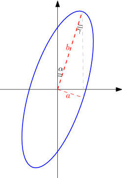
(a) A level set of $f(x,y)$

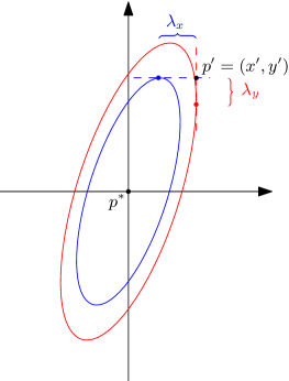
(b) Illustration of 1-d minimizers in Lemma 34

Figure 3: Illustration of the setup for Lemma 34. The figure on the left shows one level set of the quadratic form $f(x,y)$; a $\alpha$ rotation of an axis-parallel ellipse with principal axes of lengths $a$ and $b$. The figure on the right is a visual illustration of $\lambda_{x},\lambda_{y}$ in the Lemma statement. For example, the blue ellipse denotes the level set on which the minimizer $(x^{\prime\prime},y^{\prime})$ (blue dot) lies, giving $\lambda_{x}=x^{\prime}-x^{\prime\prime}$.

Lemma 34.

Let $f(x,y)$ be a quadratic form with Hessian $H=\begin{bmatrix}A^{2}&C\\ C&B^{2}\end{bmatrix}\succ 0$. Let the level sets of $f(x,y)$ be given by ellipses that are clockwise rotation by an angle $\alpha\in\left(-\frac{\pi}{4},\frac{\pi}{4}\right)$ of axis parallel ellipses: $\frac{x^{2}}{a^{2}}+\frac{y^{2}}{b^{2}}=r^{2}$. Define $\gamma$ such that $\tan\gamma=\frac{\min\{a,b\}}{\max\{a,b\}}\leq 1$.

For a given point $p^{\prime}=(x^{\prime},y^{\prime})$, define

$$x^{\prime\prime}=\mathop{\mathrm{argmin}}_{x}f(x,y^{\prime}),\qquad y^{\prime\prime}=\mathop{\mathrm{argmin}}_{x}f(x^{\prime},y),$$

and $\lambda_{x}=x^{\prime}-x^{\prime\prime}$, $\lambda_{y}=y^{\prime}-y^{\prime\prime}$. Let $p^{*}=(x^{*},y^{*})=\mathop{\mathrm{argmin}}_{(x,y)}f(x,y)$ be the true minimizer of $f(\cdot)$. If (i) $\tan\gamma\geq\frac{5}{8}$, or (ii) $|\tan\alpha|\leq\frac{\tan^{2}\gamma}{4}$, then

$$\lambda_{x}^{2}+\lambda_{y}^{2}\geq\frac{1}{2}\left\lVert p^{\prime}-p^{*}\right\rVert^{2}.$$

Proof.

We will assume that the true minimizer $p^{*}={0}$ without loss of generality, so that we need to prove that $\lambda_{x}^{2}+\lambda_{y}^{2}\geq\frac{1}{2}\cdot(x^{\prime 2}+y^{\prime 2})$. We will also assume without loss of generality that $a\leq b$. Furthermore, in the proof we will focus on the case $\alpha\in[0,\pi/4]$ and $x^{\prime},y^{\prime}\geq 0$, as illustrated in Figure 3(b). This is indeed the hardest case: if $x^{\prime}\leq 0,y^{\prime}\geq 0,0\leq\alpha\leq\pi/4$, then $|\lambda_{y}|\geq|y^{\prime}|,|\lambda_{x}|\geq x^{\prime}$ and the Lemma follows. The other cases are symmetric to one of the above.

We begin by finding an expression for $y^{\prime\prime}$. Observe that at the point $(x^{\prime},y^{\prime\prime})$, the tangent to the level set is parallel to the $y$-axis. If we now imagine rotating the level set, along with the point $(x^{\prime},y^{\prime\prime})$ counter-clockwise by an angle $\alpha$, so that the level set becomes axis-parallel and the point $(x^{\prime},y^{\prime\prime})$ moves to $(\widehat{x},\widehat{y})$, then the tangent at $(\widehat{x},\widehat{y})$ to this axis-parallel ellipse has a slope of $m=-1/\tan\alpha$. We can now obtain one relationship between $\widehat{x},\widehat{y}$ by differentiating the equation for the level set with respect to $x$:

$$\frac{d}{dx}\left.\left(\frac{x^{2}}{a^{2}}+\frac{y^{2}}{b^{2}}\right)\right|_{(\widehat{x},\widehat{y})}=0\ \implies\ \widehat{y}=\widehat{x}\frac{b^{2}}{a^{2}}\tan\alpha.$$

Let $\tan\beta:=\frac{b^{2}}{a^{2}}\tan\alpha$, so that $\widehat{y}=\widehat{x}\tan\beta$. Since $(x^{\prime},y^{\prime\prime})$ is obtained by clockwise rotation of $(\widehat{x},\widehat{y})$ by $\alpha$, we have

$$y^{\prime\prime}=x^{\prime}\tan(\beta-\alpha)=x^{\prime}\frac{\tan\beta-\tan\alpha}{1+\tan\beta\tan\alpha}.$$

Substituting $\tan\beta=\frac{b^{2}}{a^{2}}\tan\alpha=\tan\alpha/\tan^{2}\gamma$:

$$y^{\prime\prime} =x^{\prime}\tan\alpha\frac{1-\tan^{2}\gamma}{\tan^{2}\gamma+\tan^{2}\alpha}.$$ (50)

A similar analysis gives,

$$x^{\prime\prime} =y^{\prime}\tan\alpha\frac{1-\tan^{2}\gamma}{1+\tan^{2}\gamma\tan^{2}\alpha}.$$ (51)

Writing $(x^{\prime},y^{\prime})$ in polar coordinates $(r,\theta)$, we get

$$\lambda_{x} =x^{\prime}-x^{\prime\prime}=r\left(\cos\theta-\sin\theta\cdot\tan\alpha\frac{1-\tan^{2}\gamma}{1+\tan^{2}\gamma\tan^{2}\alpha}\right),$$ (52)

$$\lambda_{y} =y^{\prime}-y^{\prime\prime}=r\left(\sin\theta-\cos\theta\cdot\tan\alpha\frac{1-\tan^{2}\gamma}{\tan^{2}\gamma+\tan^{2}\alpha}\right).$$ (53)

By our assumptions, $\tan\alpha\geq 0$ and $0\leq\tan\gamma\leq 1$. One can further verify that under the condition $\tan\alpha\leq\frac{\tan^{2}\gamma}{4}$, we have

$$0\leq\tan\alpha\frac{1-\tan^{2}\gamma}{1+\tan^{2}\gamma\tan^{2}\alpha}\leq 1/4,$$

and

$$0\leq\tan\alpha\frac{1-\tan^{2}\gamma}{\tan^{2}\gamma+\tan^{2}\alpha}\leq 1/4.$$

To see why, the above inequalities can be rearranged into the following quadratic inequalities in $\tan\alpha$ for any fixed value $\tan\gamma$:

$$\left(\frac{\tan^{2}\gamma}{1-\tan^{2}\gamma}\right)\tan^{2}\alpha-4\tan\alpha+\frac{1}{1-\tan^{2}\gamma} \geq 0,$$

$$\left(\frac{1}{1-\tan^{2}\gamma}\right)\tan^{2}\alpha-4\tan\alpha+\frac{\tan^{2}\gamma}{1-\tan^{2}\gamma} \geq 0.$$

It can then be shown that $\frac{\tan^{2}\gamma}{4}$ is a lower bound on the smaller roots of the quadratic expressions on the left hand side above. In fact, the second condition above is stricter than the first (when $\tan\gamma\leq 1$), and $\frac{\tan^{2}\gamma}{4}$ is a linear approximation to the smaller root (= $2(1-\tan^{2}\gamma)-\sqrt{4\tan^{2}\gamma-9\tan\gamma+4}$) in the vicinity of $\tan^{2}\gamma=0$ for the second inequality above. In fact, if $\tan\gamma\geq\frac{5}{8}$, then the two inequalities are always true.

Finally,

$$\lambda_{x}^{2}+\lambda_{y}^{2} =(x^{\prime}-x^{\prime\prime})^{2}+(y^{\prime}-y^{\prime\prime})^{2}$$

$$\geq r^{2}\left[\sin^{2}\theta+\cos^{2}\theta-2\sin\theta\cos\theta\tan\alpha\left(\frac{1-\tan^{2}\gamma}{1+\tan^{2}\gamma\tan^{2}\alpha}+\frac{1-\tan^{2}\gamma}{\tan^{2}\gamma+\tan^{2}\alpha}\right)\right]$$

$$\geq r^{2}\left(1-\frac{1}{2}\sin 2\theta\right)\ \geq\ \frac{r^{2}}{2}.$$

∎

The Hessian for the quadratic described in Lemma 34 is given by:

$$H =\begin{bmatrix}A^{2}&C\\ C&B^{2}\end{bmatrix}\ =\begin{bmatrix}\frac{\cos^{2}\alpha}{a^{2}}+\frac{\sin^{2}\alpha}{b^{2}}&\sin\alpha\cos\alpha\left(\frac{1}{b^{2}}-\frac{1}{a^{2}}\right)\\ \sin\alpha\cos\alpha\left(\frac{1}{b^{2}}-\frac{1}{a^{2}}\right)&\frac{\sin^{2}\alpha}{a^{2}}+\frac{\cos^{2}\alpha}{b^{2}}\end{bmatrix}.$$ (54)

Lemma 35.

The Hessian in (54) satisfies the conditions of Lemma 34 if $\frac{|C|}{\min\{A^{2},B^{2}\}}\leq\frac{1}{33}$.

Proof.

Without loss of generality, assume $a\leq b$, so that with $\alpha\in[-\pi/4,\pi/4]$, we have $B^{2}\leq A^{2}$. To neaten the exposition, we will further focus on $\alpha\in[0,\pi/4]$, since only $|\sin\alpha|$ and $|\cos\alpha|$ are involved in verifying the condition.

It suffices to prove that

$$\frac{C}{B^{2}} =\frac{1}{2}\cdot\frac{\sin 2\alpha}{a^{2}/b^{2}}\cdot\frac{1-\frac{a^{2}}{b^{2}}}{1+\left(\frac{b^{2}}{a^{2}}-1\right)\sin^{2}\alpha}\ \leq\ \frac{1}{33}$$ (55)

implies $\tan\alpha\leq\frac{a^{2}}{4b^{2}}$, under the assumption that $\frac{a^{2}}{b^{2}}\leq 25/64$, since otherwise $\tan\gamma\geq 5/8$ and the first condition in Lemma 34 is satisfied. Since under this assumption $1-\frac{a^{2}}{b^{2}}\geq\frac{39}{64}$, (55) implies

$$\frac{\sin 2\alpha}{a^{2}/b^{2}}\cdot\frac{1}{1+\left(\frac{b^{2}}{a^{2}}-1\right)\sin^{2}\alpha}\ \leq\ \frac{128}{39\cdot 33}\leq\frac{1}{10}.$$

Rearranging,

$$\frac{b^{2}}{a^{2}}\leq\frac{1-\sin^{2}\alpha}{10\sin 2\alpha-\sin^{2}\alpha}\leq\frac{1-\sin^{2}\alpha}{10\sqrt{2}\sin\alpha-\sin^{2}\alpha},$$ (56)

since in the interval $\alpha\in[0,\pi/4]$ we have $\sin 2\alpha\geq\sqrt{2}\sin\alpha$. Since $\frac{b^{2}}{a^{2}}\geq\frac{64}{25}\geq 2$, we get the quadratic inequality

$$\sin^{2}\alpha-20\sqrt{2}\sin\alpha+1\geq 0,$$

which implies $\sin\alpha\leq 0.04$ and therefore $\tan\alpha=\frac{\sin\alpha}{\cos\alpha}\leq 1.01\sin\alpha$.

Starting from (56) again,

$$\left(\frac{b^{2}}{a^{2}}-1\right)\sin^{2}\alpha-10\sqrt{2}\frac{b^{2}}{a^{2}}\sin\alpha+1\geq 0,$$

which has roots $\frac{10\sqrt{2}b^{2}/a^{2}\pm\sqrt{200b^{4}/a^{4}-4b^{2}/a^{4}+4}}{2(b^{2}/a^{2}-1)}$. Since $b^{2}/a^{2}\geq 64/25$, we observe that the larger root is greater than $5\sqrt{2}$, and hence the smaller root is bounded above by $\frac{1}{5\sqrt{2}}\cdot\frac{1}{\frac{b^{2}}{a^{2}}-1}\leq\frac{64/39}{5\sqrt{2}}\cdot\frac{a^{2}}{b^{2}}$, which is also an upper bound on $\sin\alpha$. In the last inequality we have again used $b^{2}/a^{2}\geq 64/25$. Finally, $\tan\alpha\leq 1.01\sin\alpha\leq 1.01\cdot\frac{64/39}{5\sqrt{2}}\cdot\frac{a^{2}}{b^{2}}\leq\frac{a^{2}}{4b^{2}}$ as needed. ∎

The following lemma adapted from the volume argument of $\epsilon$-net w.r.t. Euclidean norm (Vershynin, 2010) gives an upper bound for the covering numbers of the sphere using $\epsilon$-net w.r.t. $\tan$.

Lemma 36.

Let $N(\epsilon,\mathbb{S}^{n-1})$ be the minimal cardinality of an $\epsilon$-net of $\mathbb{S}^{n-1}$ such that for every unit vector $v\in\mathbb{S}^{n-1}$, there exists a $v_{\epsilon}\in{\mathcal{S}}_{\epsilon}$ such that the $\tan$ of the angle between $v$ and $v_{\epsilon}$ is in $[-\epsilon,\epsilon]$. If $\epsilon\leq\frac{1}{5}$, we have that

$$N(\epsilon,\mathbb{S}^{n-1})\leq\left(1+\frac{4}{\epsilon}\right)^{n}.$$

Proof.

Choose $\mathcal{N}_{\epsilon}$ to be the maximal subset of $\mathbb{S}^{n-1}$ such that the tan of the angle between two arbitrary vectors $v_{1},v_{2}$ is larger than $\epsilon$. By the maximality property, $\mathcal{N}_{\epsilon}$ is an $\epsilon$-net. Moreover, using the fact that $x\geq\frac{1}{2}\tan(x)$ if $x\leq\frac{1}{5}$, the balls of radii $\frac{\epsilon}{4}$ centered at the points in $\mathcal{N}_{\epsilon}$ are disjoint. Let $\mathcal{B}_{n,2}$ denote the unit Euclidean ball in $\mathbb{R}^{n}$ centered at the origin. By comparing the volumes, it holds that

$$N(\epsilon,\mathbb{S}^{n-1})\cdot\left(\frac{\epsilon}{4}\right)^{n}vol(\mathcal{B}_{n})=N(\epsilon,\mathbb{S}^{n-1})\cdot vol\left(\frac{\epsilon}{4}\mathcal{B}_{n}\right)\leq vol\left(\left(1+\frac{\epsilon}{4}\right)\mathcal{B}_{n}\right)=\left(1+\frac{\epsilon}{4}\right)^{n}\cdot vol(\mathcal{B}_{n}).$$

Hence we conclude

$$N(\epsilon,\mathbb{S}^{n-1})\leq\frac{(1+\frac{\epsilon}{4})^{n}}{\frac{\epsilon}{4}^{n}}=\left(1+\frac{4}{\epsilon}\right)^{n}.$$

∎

Lemma 37.

Let $\mathcal{L}(\theta):\mathbb{R}^{n}\to\mathbb{R}$ be a quadratic form loss function with positive definite Hessian $H$ and minimizer $\theta^{*}$. Let $\kappa\geq 1$, the condition number, denote the ratio of the largest to the smallest eigenvalue of $H$. Let ${\mathcal{S}}_{\epsilon}\subset\mathbb{S}^{n-1}$ be an ‘$\epsilon$-net’ of the $n$-dimensional unit sphere so that for every unit vector $v\in\mathbb{S}^{n-1}$, there exists a $v_{\epsilon}\in{\mathcal{S}}_{\epsilon}$ such that the $\tan$ of the angle between $v$ and $v_{\epsilon}$ is in $[-\epsilon,\epsilon]$ and $\epsilon\leq\frac{1}{5+2\kappa}$. Let $\bar{\theta}$ be an approximate minimizer of $\mathcal{L}$, and let $\lambda_{v}$ denote the minimizer of the scalar quadratic function $\mathcal{L}_{v}(\lambda)=\mathcal{L}(\bar{\theta}+\lambda v)$. If for all $v_{\epsilon}\in{\mathcal{S}}_{\epsilon}$, $|\lambda_{v_{\epsilon}}|\leq\overline{\lambda}$, then $|\bar{\theta}-\theta^{*}|\leq\frac{\bar{\lambda}}{1-2(1+\kappa)\epsilon}$.

Proof.

Let $v=(v_{x},v_{y})$ denote the unit vector in the direction $\bar{\theta}-\theta^{*}$, and let $u=(u_{x},u_{y})\in{\mathcal{S}}_{\epsilon}$ satisfy the condition in the Lemma statement with respect to $v$. That is, if $m_{v}=\frac{v_{y}}{v_{x}}=\tan\alpha$ and $m_{u}=\frac{u_{y}}{u_{x}}=\tan\beta$, then $\tan(\beta-\alpha)=\epsilon^{\prime}$ with $\epsilon^{\prime}\in[-\epsilon,\epsilon]$. Let $P$ denote the point $\bar{\theta}+\lambda_{u}u$. The points $\bar{\theta},\theta^{*},P$ define a plane and the subsequent analysis will be restricted to this plane. Without loss of generality, let us translate and rotate our co-ordinate system so that $\theta^{*}$ is at the origin, the level sets of the loss function $\mathcal{L}$ restricted to the plane of interest have the form $\frac{x^{2}}{a^{2}}+\frac{y^{2}}{b^{2}}=r^{2}$ (with $\frac{1}{\kappa}\leq\frac{a^{2}}{b^{2}}\leq\kappa$), and $\bar{\theta}=(\bar{\theta}_{x},\bar{\theta}_{y})=r_{\bar{\theta}}\cdot v$ lie in the positive quadrant.

Using the fact that the point $P=\bar{\theta}+\lambda_{u}u$ is tangent to the level set, we get

$$-\lambda_{u}=\frac{\bar{\theta}_{x}b^{2}+\bar{\theta}_{y}m_{u}a^{2}}{a^{2}m_{u}^{2}+b^{2}}\cdot\sqrt{1+m_{u}^{2}}=r_{\bar{\theta}}.\frac{v_{x}b^{2}+v_{y}m_{u}a^{2}}{a^{2}m_{u}^{2}+b^{2}}\cdot\sqrt{1+m_{u}^{2}}.$$

Since $m_{u}=\tan\beta=\frac{\tan\alpha+\epsilon^{\prime}}{1-\epsilon^{\prime}\tan\alpha}=\frac{m_{v}+\epsilon^{\prime}}{1-\epsilon^{\prime}m_{v}}$, some calculations give,

$$|\lambda_{u}| =r_{\bar{\theta}}.\frac{v_{x}b^{2}+v_{y}m_{u}a^{2}}{a^{2}m_{u}^{2}+b^{2}}\cdot\sqrt{1+m_{u}^{2}}$$

$$=r_{\bar{\theta}}\sqrt{1+\epsilon^{\prime 2}}\left[1-\epsilon^{\prime}\underbrace{\frac{(m_{v}+\epsilon^{\prime})a^{2}-m_{v}(1-m_{v}\epsilon^{\prime})b^{2}}{(m_{v}+\epsilon^{\prime})^{2}a^{2}+(1-\mu\epsilon^{\prime})^{2}b^{2}}}_{D}\right].$$

We can bound $D$ as:

$$D \leq\underbrace{\frac{(m_{v}+\epsilon^{\prime})a^{2}}{(m_{v}+\epsilon^{\prime})^{2}a^{2}+(1-\mu\epsilon^{\prime})^{2}b^{2}}}_{D_{1}}+\underbrace{\frac{m_{v}|1-m_{v}\epsilon^{\prime}|b^{2}}{(m_{v}+\epsilon^{\prime})^{2}a^{2}+(1-\mu\epsilon^{\prime})^{2}b^{2}}}_{D_{2}}.$$

Assuming $|\epsilon^{\prime}|\leq\epsilon\leq 1/5$, if $m_{v}\geq 1$, then $D_{1}\leq 1$ and $D_{2}\leq\frac{2b^{2}}{a^{2}}\leq 2\kappa$. If $m_{v}\leq 1$, then $D_{1}\leq\frac{2a^{2}}{b^{2}}\leq 2\kappa$ and $D_{2}\leq 2$. Therefore, $D\leq 2(1+\kappa)$, finally giving:

$$|\bar{\theta}-\theta^{*}|=r_{\bar{\theta}}\leq\frac{|\lambda_{u}|}{\sqrt{1+\epsilon^{\prime 2}}}\cdot\frac{1}{1-2(1+\kappa)\epsilon^{\prime}}\leq\frac{\bar{\lambda}}{1-2(1+\kappa)\epsilon}.$$

∎

C.4 Bound on $\sum_{t\in{\mathcal{I}}}\left\lVert z_{t}\right\rVert^{2}$

Lemma 38.

For a $\delta\in(0,1)$ and an interval ${\mathcal{I}}$ lying within some block $\mathcal{B}_{ij}$ with $j\geq 1$ and $|{\mathcal{I}}|\geq 16\ln\frac{1}{\delta}$, it holds with probability at least $1-\delta$ that

$$\sum_{t\in{\mathcal{I}}}\left\lVert z_{t}\right\rVert^{2}\leq|{\mathcal{I}}|\left(2\left((1+K_{u}^{2})\max_{t\in{\mathcal{I}}}\left\lVert x_{t}\right\rVert^{2}+2\sigma_{L}^{2}\right)\right).$$

In particular, for any $\bar{x}\geq 0$, conditioned on $\max_{t\in{\mathcal{I}}}\left\lVert x_{t}\right\rVert\leq\bar{x}$, we have $\sum_{t\in{\mathcal{I}}}\left\lVert z_{t}\right\rVert^{2}\leq|{\mathcal{I}}|\bar{z}$, where $\bar{z}:=\sqrt{2\left((1+K_{u}^{2})\bar{x}^{2}+2\sigma_{L}^{2}\right)}$. Here $\sigma^{2}_{L}:=\nu^{2}_{1}=\sqrt{C_{0}/2L}$.

Proof.

Recall that $z_{t}=y_{t}+\xi_{t}$ and $\left\lVert K_{t}\right\rVert,\left\lVert K_{t}^{\textsf{stab}}\right\rVert\leq K_{u}$. We have

$$\sum_{t\in{\mathcal{I}}}\left\lVert z_{t}\right\rVert^{2} =\sum_{t\in{\mathcal{I}}}\left\lVert y_{t}+\xi_{t}\right\rVert^{2}$$

$$\leq 2\sum_{t\in{\mathcal{I}}}\left\lVert y_{t}\right\rVert^{2}+2\sum_{t\in{\mathcal{I}}}\left\lVert\xi_{t}\right\rVert^{2}$$

$$\leq 2(1+K_{u}^{2})|{\mathcal{I}}|\max_{t\in{\mathcal{I}}}\left\lVert x_{t}\right\rVert^{2}+2\sum_{t\in{\mathcal{I}}}\left\lVert\xi_{t}\right\rVert^{2}.$$

By a standard Laurent-Massart bound, we have:

$$\text{{\bf Pr}$\left[\sum_{t\in{\mathcal{I}}}\left\lVert\xi_{t}\right\rVert^{2}\geq\sigma_{L}^{2}\left(|{\mathcal{I}}|+2\sqrt{|{\mathcal{I}}|\ln\left(\frac{1}{\delta}\right)}+2\ln\left(\frac{1}{\delta}\right)\right)\right]$}\leq\delta.$$

Using the fact that $\left(|{\mathcal{I}}|+2\sqrt{|{\mathcal{I}}|\ln(\frac{1}{\delta})}+2\ln(\frac{1}{\delta})\right)\leq 2|{\mathcal{I}}|$ when $|{\mathcal{I}}|\geq 16\ln\frac{1}{\delta}$, plugging the above in the bound derived above for $\sum_{t}\left\lVert z_{t}\right\rVert^{2}$ indicates that

$$\sum_{t\in{\mathcal{I}}}\left\lVert z_{t}\right\rVert^{2} \leq 2\left((1+K_{u}^{2})\max_{t\in{\mathcal{I}}}\left\lVert x_{t}\right\rVert^{2}+2\sigma_{L}^{2}\right)|{\mathcal{I}}|$$

holds with probability at least $1-\delta$. The right hand side of the bound given above is a random variable since it involves $\max_{t\in{\mathcal{I}}}\left\lVert x_{t}\right\rVert$, and can instead be interpreted as saying that for any $\bar{x}$, conditioned on the event $\max_{t\in{\mathcal{I}}}\left\lVert x_{t}\right\rVert\leq\bar{x}$, $\sum_{t\in{\mathcal{I}}}\left\lVert z_{t}\right\rVert^{2}\leq 2\left((1+K_{u}^{2})\bar{x}^{2}+2\sigma_{L}^{2}\right)|{\mathcal{I}}|=:|{\mathcal{I}}|\bar{z}$. ∎

Definition 39.

Define $z_{u}:=\sqrt{2\left((1+K_{u}^{2})x_{u}^{2}+2\sigma_{L}^{2}\right)}$, where $x_{u}$ is defined in Algorithm 1.

C.5 Bound on the condition number of $\sum_{t\in{\mathcal{I}}}z_{t}z_{t}^{\top}$

Lemma 40.

For an arbitrary interval ${\mathcal{I}}$, denote design matrix $\Upsilon_{\mathcal{I}}=\sum_{t\in{\mathcal{I}}}z_{t}z_{t}^{\top}$ and its condition number $\kappa=\lambda_{max}(\Upsilon_{\mathcal{I}})/\lambda_{min}(\Upsilon_{{\mathcal{I}}})$.

(i) Let ${\mathcal{I}}$ be an interval within a block $\mathcal{B}_{i,j}$ in Algorithm 1. Define $\bar{x}=\max_{t\in{\mathcal{I}}}\left\lVert x_{t}\right\rVert$, and $\bar{z}$ as in Lemma 38. If we have

$$|{\mathcal{I}}| \geq\frac{2000}{9}\left(2(n+d)\log\frac{1}{\delta}+(n+d)\log\frac{\bar{x}^{2}(1+\left\lVert K\right\rVert^{2})+\sigma_{L}^{2}}{{\sigma}^{2}_{\mathcal{I}}\min\left\{\frac{1}{2},\frac{\psi^{2}}{{\sigma}^{2}_{L}+2\left\lVert K\right\rVert^{2}}\right\}}\right),$$

then for $\delta\leq 3/100$, it holds with probability at least $1-3\delta$ that the condition number is upper bounded as

$$\kappa\leq\frac{\bar{z}^{2}|{\mathcal{I}}|}{\frac{9|{\mathcal{I}}|}{1600}{\sigma}^{2}_{\mathcal{I}}\min\left\{\frac{1}{2},\frac{\psi^{2}}{{\sigma}^{2}_{L}+2\left\lVert K\right\rVert^{2}}\right\}}=\frac{1600\bar{z}^{2}}{9{\sigma}^{2}_{\mathcal{I}}\min\left\{\frac{1}{2},\frac{\psi^{2}}{{\sigma}^{2}_{L}+2\left\lVert K\right\rVert^{2}}\right\}}.$$

Define $\kappa_{\mathcal{I}}$ be the bound above when $\bar{x}=x_{u}$:

$$\kappa_{{\mathcal{I}}}\coloneqq\frac{1600z_{u}^{2}}{9{\sigma}^{2}_{\mathcal{I}}\min\left\{\frac{1}{2},\frac{\psi^{2}}{{\sigma}^{2}_{L}+2\left\lVert K\right\rVert^{2}}\right\}},$$

whence it follows that $\kappa_{{\mathcal{I}}}\leq C_{9}\sqrt{|{\mathcal{I}}|}$ for some problem-dependent constant (independent of $T$) $C_{9}$.

(ii) For any warm-up block $\mathcal{B}_{i,0}$ in in Algorithm 1, with sequentially strongly stablizing policies $\{K_{t}^{\textsf{stab}}\}$ such that $\left\lVert K_{t}^{\textsf{stab}}\right\rVert\leq K_{u}$, if

$$|\mathcal{B}_{i,0}| \geq\frac{2000}{9}\left(2(n+d)\log\frac{1}{\delta}+(n+d)\log\frac{\bar{x}^{2}(1+K_{u}^{2})+\sigma_{0}^{2}}{{\sigma}^{2}_{0}\min\left\{\frac{1}{2},\frac{\psi^{2}}{{\sigma}^{2}_{0}+2(K_{l}^{\textsf{stab}})^{2}}\right\}}\right),$$

we have for $\delta\leq 3/100$,

$$\kappa\leq\frac{\bar{z}^{2}|\mathcal{B}_{i,0}|}{\frac{9|\mathcal{B}_{i,0}|}{1600}{\sigma}^{2}_{0}\min\left\{\frac{1}{2},\frac{\psi^{2}}{{\nu}^{2}_{0}+2\left\lVert K\right\rVert^{2}}\right\}}=\frac{1600\bar{z}^{2}}{9{\nu}^{2}_{0}\min\left\{\frac{1}{2},\frac{\psi^{2}}{{\nu}^{2}_{0}+2\left\lVert K\right\rVert^{2}}\right\}}.$$

Define $\kappa_{0}$ to be the bound above when $\bar{x}=x_{u}$:

$$\kappa_{0}\coloneqq\frac{1600z_{u}^{2}}{9{\nu}^{2}_{0}\min\left\{\frac{1}{2},\frac{\psi^{2}}{{\nu}^{2}_{0}+2\left\lVert K\right\rVert^{2}}\right\}},$$

from where it follows that $\kappa_{0}\leq C_{10}\ln T$ for some problem dependent constant $C_{10}$.

Proof.

We need to bound $\lambda_{\min}(\Upsilon_{\mathcal{I}})$ and $\lambda_{\max}(\Upsilon_{\mathcal{I}})$ separately. By direct computation and Lemma 38, it holds with probability at least $1-\delta$ that

$$\lambda_{\max}(\Upsilon_{\mathcal{I}})\leq\mathop{\mathrm{Tr}}(\Upsilon_{\mathcal{I}})=\sum_{t\in{\mathcal{I}}}z_{t}z_{t}^{\top}=\sum_{t\in{\mathcal{I}}}\left\lVert z_{t}\right\rVert^{2}\leq\bar{z}^{2}|{\mathcal{I}}|.$$

In the sequel, we bound $\lambda_{\min}(\Upsilon_{\mathcal{I}})$ from below by specifying the choice of $\Upsilon_{0}$ such that $\Upsilon_{0}\preceq\Upsilon_{\mathcal{I}}$ with high probability using Lemma 41. Note that $z_{t}\mid\mathcal{F}_{t-1}\sim\mathcal{N}\left(\overline{z}_{t},\Sigma_{t}\right)$, where $\overline{z}_{t}$ and $\Sigma_{t}$ are measurable and

$$\Sigma_{t}\succeq\left[\begin{array}[]{cc}\psi^{2}I_{n}&\psi^{2}I_{n}K^{\top}\\ \psi^{2}KI_{n}&\psi^{2}KI_{d}K^{\top}+{\sigma}^{2}_{t}I_{d}\end{array}\right].$$

By Dean et al. (2018, Lemma F. 6), we have

$$\lambda_{\min}\left(\Sigma_{t}\right)\geq{\sigma}^{2}_{t}\min\left\{\frac{1}{2},\frac{\psi^{2}}{{\sigma}^{2}_{t}+2\left\lVert K\right\rVert^{2}}\right\}\geq{\sigma}^{2}_{\mathcal{I}}\min\left\{\frac{1}{2},\frac{\psi^{2}}{{\sigma}^{2}_{L}+2\left\lVert K\right\rVert^{2}}\right\}.$$

Moreover, we have

$$\mathop{\mathrm{Tr}}\left(\text{{\bf E}$\left[\Upsilon_{\mathcal{I}}\right]$}\right) =\text{{\bf E}$\left[\sum_{t\in{\mathcal{I}}}\left\|{x}_{t}\right\|^{2}+\left\|{u}_{t}\right\|^{2}\right]$}$$

$$\leq\text{{\bf E}$\left[\sum_{t\in{\mathcal{I}}}\left\|{x}_{t}\right\|^{2}+\|K_{t}\|^{2}\left\|{x}_{t}\right\|^{2}+\sigma_{L}^{2}\right]$}$$

$$\leq|{\mathcal{I}}|\left(\bar{x}^{2}(1+\left\lVert K\right\rVert^{2})+\sigma_{L}^{2}\right).$$

Setting $\mathcal{E}=\Omega$ (the probability space) and

$$\Upsilon_{0}=\frac{9|{\mathcal{I}}|}{1600}{\sigma}^{2}_{\mathcal{I}}\min\left\{\frac{1}{2},\frac{\psi^{2}}{{\sigma}^{2}_{L}+2\left\lVert K\right\rVert^{2}}\right\}I_{d+n},$$

Lemma 41 implies if

$$|{\mathcal{I}}| \geq\frac{2000}{9}\left(2(n+d)\log\frac{100}{3}+(n+d)\log\frac{\bar{x}^{2}(1+\left\lVert K\right\rVert^{2})+\sigma_{L}^{2}}{{\sigma}^{2}_{\mathcal{I}}\min\left\{\frac{1}{2},\frac{\psi^{2}}{{\sigma}^{2}_{L}+2\left\lVert K\right\rVert^{2}}\right\}}\right)$$ (57)

$$\geq\frac{2000}{9}\left(2(n+d)\log\frac{1}{\delta}+(n+d)\log\frac{\bar{x}^{2}(1+\left\lVert K\right\rVert^{2})+\sigma_{L}^{2}}{{\sigma}^{2}_{\mathcal{I}}\min\left\{\frac{1}{2},\frac{\psi^{2}}{{\sigma}^{2}_{L}+2\left\lVert K\right\rVert^{2}}\right\}}\right)$$ (58)

with $\delta\leq 3/100$, we have

$$\mathbb{P}\left[\Upsilon_{T}\nsucceq\Upsilon_{0}\right] \leq 2\exp(-\frac{9}{2000((n+d)+1)}|{\mathcal{I}}|)$$

$$\leq 2\exp\left(-\frac{9}{2000((n+d)+1)}\frac{2000}{9}\left(2(n+d)\log\frac{1}{\delta}\right)\right)$$

$$\leq 2\exp\left(-\frac{9}{2000((n+d)+1)}\frac{2000}{9}\left((n+d+1)\log\frac{1}{\delta}\right)\right)$$

$$=2\delta.$$

Then it holds with probability at least $1-2\delta-\delta=1-3\delta$ that

$$\kappa\leq\frac{\bar{z}^{2}|{\mathcal{I}}|}{\frac{9|{\mathcal{I}}|}{1600}{\sigma}^{2}_{\mathcal{I}}\min\left\{\frac{1}{2},\frac{\psi^{2}}{{\sigma}^{2}_{L}+2\left\lVert K\right\rVert^{2}}\right\}}=\frac{1600\bar{z}^{2}}{9{\sigma}^{2}_{\mathcal{I}}\min\left\{\frac{1}{2},\frac{\psi^{2}}{{\sigma}^{2}_{L}+2\left\lVert K\right\rVert^{2}}\right\}}.$$ (59)

For a warm-up block $\mathcal{B}_{i,0}$, note that the exploration noise is fixed at $\nu_{0}^{2}=1$, and we have $\left\|K_{t}^{\text{stab }}\right\|\leq K_{u}$. Plugging these parameters into (57) and (59) yields the corresponding results. ∎

C.6 Supporting Lemmas

Lemma 41 (Lemma E.4 in Simchowitz and Foster (2020)).

Suppose $z_{t}\mid\mathcal{F}_{t-1}\sim\mathcal{N}\left(\overline{z}_{t},\Sigma_{t}\right)$, where $\overline{z}_{t}\in\mathbb{R}^{\widetilde{d}}$ and $\Sigma_{t}\in\mathbb{R}^{\widetilde{d}\times\widetilde{d}}$ are $\mathcal{F}_{t-1}$-measurable, and $\Sigma_{t}\succeq\Sigma\succ 0$. Suppose $\mathcal{E}$ is an arbitrary event and suppose $\mathop{\mathrm{Tr}}\left(\text{{\bf E}$\left[V_{\mathcal{I}}\mathbbm{1}\{\mathcal{E}\}\right]$}\right)\leq\Lambda T$ for some constant $\Lambda\geq 0$. Then for

$$T\geq\frac{2000}{9}(2\widetilde{d}\log(\frac{100}{3})+\widetilde{d}\log\frac{\Lambda}{\lambda_{\min}(\Sigma)}),$$

let $V_{0}\coloneqq\frac{9T}{1600}\Sigma$, it holds that

$$\text{{\bf Pr}$\left[\{V_{T}\nsucceq V_{0}\}\cap\mathcal{E}\right]$}\leq 2\exp\left(-\frac{9}{2000(\widetilde{d}+1)}T\right).$$

Lemma 42 (Self-Normalized Tail Bound (Abbasi-Yadkori et al., 2011)).

Let $\{\eta_{t}\}_{t\geq 1}$ be a $\mathcal{F}_{t}$-adapted sequence such that $\eta_{t}\mid\mathcal{F}_{t-1}$ is $\sigma^{2}$-sub-Gaussian. Define $V_{T}\coloneqq\sum_{t=1}^{T}z_{t}z_{t}^{\top}$. Fix $V_{0}\succ 0$, it holds with probability $1-\delta$ that

$$\left\|\sum_{t=1}^{T}\mathbf{x}_{t}\eta_{t}\right\|_{\left(V_{0}+V_{T}\right)^{-1}}^{2}\leq 2\sigma^{2}\log\left\{\frac{1}{\delta}\operatorname{det}\left(V_{0}^{-1/2}\left(V_{0}+V_{T}\right)V_{0}^{-1/2}\right)\right\}.$$

Appendix D Proof of Proposition 12

Consider a non-stationary Markov decision process on state space ${\mathcal{S}}$ and action space $\mathcal{A}$, with a time-invariant cost function $c(\cdot,\cdot):{\mathcal{S}}\times\mathcal{A}\to\mathbb{R}$, and time-dependent transition kernel parametrized by $\{\Theta_{t}\}_{t\in[T]}$. Let $J^{*}_{t}$ denote the optimal (minimum) average cost of the MDP corresponding to $\Theta_{t}$, and let $h_{t}(\cdot):{\mathcal{S}}\to\mathbb{R}$ denote the relative value (bias) function. Then for an arbitrary state $s_{t}\in{\mathcal{S}}$ and action $a_{t}\in\mathcal{A}$, we have the inequality:

$$c(s_{t},a_{t})\geq J^{*}_{t}+h_{t}(s_{t})-\text{{\bf E}${}_{\Theta_{t}}\left[h(s_{t+1})\mid s_{t},a_{t}\right]$},$$ (60)

where E${}_{\Theta_{t}}\left[X\right]$ denotes the expectation of random variable $X$ under transition kernel parametrized by $\Theta_{t}$. Summing the above inequality from $t=1$ to $T$:

$$\sum_{t=1}^{T}c(s_{t},a_{t}) \geq\sum_{t=1}^{T}J^{*}_{t}+h_{t}(s_{t})-\text{{\bf E}${}_{\Theta_{t}}\left[h(s_{t+1})\mid s_{t},a_{t}\right]$}$$

$$=\sum_{t=1}^{T}J^{*}_{t}+h_{1}(s_{1})-\text{{\bf E}${}_{\Theta_{T}}\left[h_{T}(s_{T+1})\mid s_{T},a_{T}\right]$}$$

$$\qquad+\sum_{t=1}^{T-1}h_{t+1}(s_{t+1})-\text{{\bf E}${}_{\Theta_{t}}\left[h_{t}(s_{t+1})\mid s_{t},a_{t}\right]$}$$

$$=\sum_{t=1}^{T}J^{*}_{t}+h_{1}(s_{1})-\text{{\bf E}${}_{\Theta_{T}}\left[h_{T}(s_{T+1})\mid s_{T},a_{T}\right]$}$$

$$\qquad+\sum_{t=1}^{T-1}h_{t+1}(s_{t+1})-\text{{\bf E}${}_{\Theta_{t}}\left[h_{t+1}(s_{t+1})\mid s_{t},a_{t}\right]$}$$

$$\qquad+\sum_{t=1}^{T-1}\text{{\bf E}${}_{\Theta_{t}}\left[h_{t+1}(s_{t+1})-h_{t}(s_{t+1})\mid s_{t},a_{t}\right]$}.$$

Taking expectation with respect to the randomization of the policy and the evolution of the non-stationary MDP,

$$\text{{\bf E}$\left[\sum_{t=1}^{T}c(s_{t},a_{t})\right]$}-\sum_{t=1}^{T}J^{*}_{t} \geq h_{1}(s_{1})-\text{{\bf E}$\left[h_{T}(s_{T+1})\right]$}+\sum_{t=1}^{T-1}\text{{\bf E}$\left[h_{t+1}(s_{t+1})-h_{t}(s_{t+1})\right]$}$$

or

$$\sum_{t=1}^{T}J^{*}_{t}-\text{{\bf E}$\left[\sum_{t=1}^{T}c(s_{t},a_{t})\right]$} \leq-h_{1}(s_{1})+\text{{\bf E}$\left[h_{T}(s_{T+1})\right]$}+\sum_{t=1}^{T-1}\text{{\bf E}$\left[h_{t}(s_{t+1})-h_{t+1}(s_{t+1})\right]$}.$$

Specializing to the non-stationary LQR setting, $s_{t}\equiv x_{t}$, $a_{t}\equiv u_{t}$, $c(x_{t},u_{t})=x_{t}^{\top}Qx_{t}+u_{t}^{\top}Ru_{t}$, $h_{t}(s_{t})\equiv x_{t}^{\top}P^{*}_{t}x_{t}$:

$$\sum_{t=1}^{T}J^{*}_{t}-\text{{\bf E}$\left[\sum_{t=1}^{T}c(x_{t},u_{t})\right]$} \leq\text{{\bf E}$\left[x_{T+1}^{\top}P_{T}^{*}x_{T+1}\right]$}+\sum_{t=1}^{T-1}\text{{\bf E}$\left[x_{t+1}^{\top}\left(P_{t}^{*}-P_{t+1}^{*}\right)x_{t+1}\right]$}$$

$$\leq\text{{\bf E}$\left[\left\lVert x_{T+1}\right\rVert^{2}\right]$}\left\lVert P_{T}^{*}\right\rVert+\sum_{t=1}^{T-1}\text{{\bf E}$\left[\left\lVert x_{t+1}\right\rVert^{2}\right]$}\left\lVert P_{t}^{*}-P_{t+1}^{*}\right\rVert.$$

In Lemma 43, we prove that under the optimal dynamic policy, E$\left[\left\lVert x_{t}\right\rVert^{2}\right]$ is bounded from above by a constant depending only on the cost parameters and the sequential stability parameters $\kappa,\gamma$. The perturbation result for the solution of Discrete Algebraic Riccati equation gives $\left\lVert P_{t}^{*}-P_{t+1}^{*}\right\rVert\leq\min\{2C_{4}\left\lVert\Theta_{t}-\Theta_{t+1}\right\rVert^{2},2P_{u}\}=\mathcal{O}(\Delta^{2}_{t+1})$ (Simchowitz and Foster, 2020, Theorem 5). Lemma 43 does not bound E$\left[\left\lVert x_{T+1}\right\rVert^{2}\right]$, however, following a similar argument as in the Lemma, we can create another policy that has logarithmic regret compared to the optimal policy and has bounded E$\left[\left\lVert x_{T+1}\right\rVert^{2}\right]$. Combining these, we get the desired bound on the additional regret of $\mathcal{O}(V_{T}+\log T)$ with respect to the dynamic optimal policy. $\Box$

Lemma 43.

Under the optimal dynamic policy for the non-stationary LQR problem,

$$q_{\min}\text{{\bf E}$\left[\left\lVert x_{t}\right\rVert^{2}\right]$}\leq M_{\Gamma}\frac{2\kappa^{2}}{\gamma}M_{x}+M_{P}\frac{2\kappa^{2}}{\gamma}+\left(\kappa^{2}M_{x}+\frac{2\kappa^{2}n\psi^{2}}{\gamma}\right)\left(\frac{2\kappa^{2}}{\gamma}M_{\Gamma}+\kappa^{2}M_{P}\right),$$

where $M_{x}:=\left(\frac{M_{\Gamma}}{q_{\min}}\right)\frac{2\kappa^{2}n\psi^{2}}{\gamma}$, $M_{P}:=\frac{2n\kappa^{2}}{\gamma}M_{\Gamma}$, and $M_{\Gamma}:=\max_{s}\left\lVert Q+(K_{s}^{\textsf{stab}})^{\top}RK_{s}^{\textsf{stab}}\right\rVert\leq q_{\max}+r_{\max}\kappa^{2}$.

Proof.

We prove this result by contradiction. We first establish some notation for the optimal dynamic policy. A classical fact is that the optimal dynamic policy for non-stationary LQR is also a linear state feedback policy, given via the following dynamic programming recursion:

$$P_{T+1} =0,$$

$$K_{t} =-(R+B_{t}^{\top}P_{t+1}B_{t})B_{t}^{\top}P_{t+1}A_{t},$$

$$P_{t} =Q+K_{t}^{\top}RK_{t}+(A_{t}+B_{t}K_{t})^{\top}P_{t+1}(A_{t}+B_{t}K_{t}),$$

$$J_{t} =\mathop{\mathrm{Tr}}(W\cdot P_{t+1}).$$

Let $t$ be some time such that under the optimal dynamic policy, E$\left[\left\lVert x_{t}\right\rVert^{2}\right]$ is larger than the bound in the Lemma statement. Define

$$\tau=\max\{s\leq t-1:\text{{\bf E}$\left[\left\lVert x_{s}\right\rVert^{2}\right]$}\leq M_{x}\}$$

as the last time before $t$ when the expected squared norm of the state under the optimal policy is smaller than $M_{x}$. Similarly, define

$$\tau^{\prime}=\min\{s\geq t:\left\lVert P_{s+1}\right\rVert\leq M_{P}\}$$

as the first time including or after $t$ when the norm of $P_{s+1}$ is smaller than $M_{P}$. We will show that by deviating to a policy where $K^{\prime}_{s}=K_{s}^{\textsf{stab}}$ for $s\in\{\tau,\ldots,\tau^{\prime}\}$ gives a policy with a smaller cost. Let $\{x^{\prime}_{s}\}$ denote the state process for this new policy, $\{P^{\prime}_{s}\}$ the relative value function matrices, and $J^{\prime}_{s}:=\mathop{\mathrm{Tr}}(W\cdot P^{\prime}_{s})$.

By the definition of the new policy, we must have $P^{\prime}_{s}=P_{s}$ for $s\geq\tau^{\prime}+1$. Recall the recursion for the relative value function for LQR:

$$x_{t}^{\top}Qx_{t}+u_{t}^{\top}Ru_{t}=x_{t}^{\top}P_{t}x_{t}+J_{t}-\text{{\bf E}$\left[x_{t+1}^{T}P_{t+1}x_{t+1}\right]$}.$$

We will decompose the cost of the optimal policy into contributions due to the four intervals $\{1,\ldots,\tau-1\}$, $\{\tau,\ldots,t\}$, $\{t+1,\ldots,\tau^{\prime}\}$ and $\{\tau^{\prime}+1,\ldots,T\}$. Since both policies agree on the first interval, the total cost is the same, and hence we do not consider it henceforth. For the interval $\{\tau,\ldots,t\}$ we lower bound the cost of the optimal policy as:

E$$\left[\sum_{s=\tau}^{t}x_{s}^{\top}Qx_{s}+u_{s}^{\top}Ru_{s}\right] \geq\sum_{s=\tau}^{t}q_{\min}\text{{\bf E}$\left[\left\lVert x_{s}\right\rVert^{2}\right]$}.$$ (61)

For the interval $\{t+1\ldots,\tau^{\prime}\}$:

E$$\left[\sum_{s=t+1}^{\tau^{\prime}}x_{s}^{\top}Qx_{s}+u_{s}^{\top}Ru_{s}\right] =\text{{\bf E}$\left[x_{t+1}^{\top}P_{t+1}x_{t+1}\right]$}+\sum_{s=t+1}^{\tau^{\prime}}J_{s}-\text{{\bf E}$\left[x_{\tau^{\prime}+1}^{\top}P_{\tau^{\prime}+1}x_{\tau^{\prime}+1}\right]$}$$

$$\geq\sum_{s=t+1}^{\tau^{\prime}+1}\mathop{\mathrm{Tr}}(W\cdot P_{s})-\text{{\bf E}$\left[x_{\tau^{\prime}+1}^{\top}P_{\tau^{\prime}+1}x_{\tau^{\prime}+1}\right]$},$$

where we have used $\text{{\bf E}$\left[x_{t+1}^{\top}P_{t+1}x_{t+1}\right]$}\geq\text{{\bf E}$\left[w_{t+1}^{\top}P_{t+1}w_{t+1}\right]$}=\mathop{\mathrm{Tr}}(W\cdot P_{t+1})$. Finally, for the last interval,

E$$\left[\sum_{s=\tau^{\prime}+1}^{T}x_{s}^{\top}Qx_{s}+u_{s}^{\top}Ru_{s}\right] =\text{{\bf E}$\left[x_{\tau^{\prime}+1}^{\top}P_{\tau^{\prime}+1}x_{\tau^{\prime}+1}\right]$}+\sum_{s=\tau^{\prime}+1}^{T}J_{s}.$$

It will be convenient to combine the lower bound for the interval $\{t+1,\ldots,T\}$ as:

E$$\left[\sum_{s=t+1}^{T}x_{s}^{\top}Qx_{s}+u_{s}^{\top}Ru_{s}\right] \geq\sum_{s=t+1}^{\tau^{\prime}}\mathop{\mathrm{Tr}}(W\cdot P_{s})+\sum_{s=\tau^{\prime}}^{T}J_{s}$$

$$\geq\sum_{t=t+1}^{\tau^{\prime}}\psi^{2}\left\lVert P_{s}\right\rVert+\sum_{s=\tau^{\prime}}^{T}J_{s}.$$ (62)

We now proceed to upper bound the cost during these intervals for the modified policy $\{K^{\prime}_{s}\}$. Denote $u^{\prime}_{s}=K^{\prime}_{s}x^{\prime}_{s}$ as the control at time step $s$ under the new policy. We first summarize the results of Lemma 44, which bounds E$\left[\left\lVert x^{\prime}_{s}\right\rVert^{2}\right]$ and $\left\lVert P^{\prime}_{s}\right\rVert$ for $s\in\{\tau+1,\ldots,\tau^{\prime}\}$:

E$$\left[\left\lVert x_{s}\right\rVert^{2}\right] \leq\kappa^{2}\left(1-\frac{\gamma}{2}\right)^{2(s-\tau)}\text{{\bf E}$\left[\left\lVert x_{\tau}\right\rVert^{2}\right]$}+\frac{2\kappa^{2}n\psi^{2}}{\gamma},$$

$$\left\lVert P^{\prime}_{s}\right\rVert \leq\kappa^{2}\left(1-\frac{\gamma}{2}\right)^{2(\tau^{\prime}-s+1)}\left\lVert P_{\tau^{\prime}+1}\right\rVert+\frac{2\kappa^{2}}{\gamma}M_{\Gamma}.$$

For the second interval, $\{\tau,\ldots,t\}$, we can upper bound the cost of the new policy by:

E$$\left[\sum_{s=\tau}^{t}{x^{\prime}}_{s}^{\top}Qx^{\prime}_{s}+{u^{\prime}}_{s}^{\top}Ru^{\prime}_{s}\right] =\text{{\bf E}$\left[\sum_{s=\tau}^{t}{x^{\prime}}_{s}^{\top}(Q+{K^{\prime}}_{s}^{\top}RK^{\prime}_{s})x^{\prime}_{s}\right]$}$$

$$\leq M_{\Gamma}\sum_{s=\tau}^{t}\text{{\bf E}$\left[\left\lVert x^{\prime}_{s}\right\rVert^{2}\right]$}$$

$$\leq M_{\Gamma}\left((t-\tau)\frac{2\kappa^{2}n\psi^{2}}{\gamma}+\frac{2\kappa^{2}}{\gamma}\text{{\bf E}$\left[\left\lVert x_{\tau}\right\rVert^{2}\right]$}\right),$$ (63)

where we have used the bound on E$\left[\left\lVert x^{\prime}_{s}\right\rVert^{2}\right]$ from Lemma 44. Next, we upper bound the cost for interval $\{t+1,\ldots,T\}$:

E$$\left[\sum_{s=t+1}^{\tau^{\prime}}{x^{\prime}}_{s}^{\top}Qx^{\prime}_{s}+{u^{\prime}}_{s}^{\top}Ru^{\prime}_{s}\right] =\text{{\bf E}$\left[{x^{\prime}_{t+1}}^{\top}P^{\prime}_{t+1}x^{\prime}_{t+1}\right]$}+\sum_{s={t+1}}^{T}J^{\prime}_{s}$$

$$=\text{{\bf E}$\left[{x^{\prime}_{t+1}}^{\top}P^{\prime}_{t+1}x^{\prime}_{t+1}\right]$}+\sum_{s=t+2}^{\tau^{\prime}}\mathop{\mathrm{Tr}}(W\cdot P^{\prime}_{s})+\sum_{s={\tau^{\prime}}}^{T}J^{\prime}_{s}$$

$$\leq\text{{\bf E}$\left[\left\lVert x^{\prime}_{t+1}\right\rVert^{2}\right]$}\left\lVert P^{\prime}_{t+1}\right\rVert+n\psi^{2}\sum_{s={t+2}}^{\tau^{\prime}}\left\lVert P^{\prime}_{s}\right\rVert+\sum_{s=\tau^{\prime}}^{T}J_{s}.$$

Using Lemma 44 we can bound:

$$\sum_{s={t+2}}^{\tau^{\prime}}\left\lVert P^{\prime}_{s}\right\rVert\leq\sum_{s={t+2}}^{\tau^{\prime}}\left(\kappa^{2}\left(1-\frac{\gamma}{2}\right)^{2(\tau^{\prime}-s+1)}\left\lVert P_{\tau^{\prime}+1}\right\rVert+\frac{2\kappa^{2}}{\gamma}M_{\Gamma}\right)\leq(\tau^{\prime}-t-1)\frac{2\kappa^{2}}{\gamma}M_{\Gamma}+\frac{2\kappa^{2}}{\gamma}\left\lVert P_{\tau^{\prime}+1}\right\rVert.$$

Also, using Lemma 44:

$$\text{{\bf E}$\left[\left\lVert x^{\prime}_{t+1}\right\rVert^{2}\right]$}\left\lVert P^{\prime}_{t+1}\right\rVert\leq\left(\kappa^{2}\text{{\bf E}$\left[\left\lVert x_{\tau}\right\rVert^{2}\right]$}+\frac{2\kappa^{2}n\psi^{2}}{\gamma}\right)\left(\kappa^{2}\left\lVert P_{\tau^{\prime}+1}\right\rVert+\frac{2\kappa^{2}}{\gamma}M_{\Gamma}\right).$$

Putting together,

E$$\left[\sum_{s=t+1}^{\tau^{\prime}}{x^{\prime}}_{s}^{\top}Qx^{\prime}_{s}+{u^{\prime}}_{s}^{\top}Ru^{\prime}_{s}\right] \leq\left(\kappa^{2}\text{{\bf E}$\left[\left\lVert x_{\tau}\right\rVert^{2}\right]$}+\frac{2\kappa^{2}n\psi^{2}}{\gamma}\right)\left(\kappa^{2}\left\lVert P_{\tau^{\prime}+1}\right\rVert+\frac{2\kappa^{2}}{\gamma}M_{\Gamma}\right)$$

$$\qquad+n\psi^{2}\left((\tau^{\prime}-t)\frac{2\kappa^{2}}{\gamma}M_{\Gamma}+\frac{2\kappa^{2}}{\gamma}\left\lVert P_{\tau^{\prime}+1}\right\rVert\right)+\sum_{s=\tau^{\prime}+1}^{T}J_{s}.$$ (64)

Combining the lower bounds on the optimal policy cost from (61)-(62) and upper bound on the cost of the modified policy from (63)-(64):

$$\text{{\bf E}$\left[\sum_{s=\tau}^{T}{x}_{s}^{\top}Qx_{s}+{u}_{s}^{\top}Ru_{s}\right]$}-\text{{\bf E}$\left[\sum_{s=\tau}^{T}{x^{\prime}}_{s}^{\top}Qx^{\prime}_{s}+{u^{\prime}}_{s}^{\top}Ru^{\prime}_{s}\right]$}$$

$$\geq \ \sum_{s=\tau}^{t-1}\left(q_{\min}\text{{\bf E}$\left[\left\lVert x_{t}\right\rVert^{2}\right]$}-M_{\Gamma}\frac{2\kappa^{2}n\psi^{2}}{\gamma}\right)$$

$$\qquad+\psi^{2}\sum_{s=t+1}^{\tau^{\prime}}\left(\left\lVert P_{s}\right\rVert-\frac{2\kappa^{2}n}{\gamma}M_{\Gamma}\right)$$

$$\qquad+q_{\min}\text{{\bf E}$\left[\left\lVert x_{t}\right\rVert^{2}\right]$}-\frac{2\kappa^{2}}{\gamma}\left\lVert P_{\tau^{\prime}+1}\right\rVert-M_{\Gamma}\frac{2\kappa^{2}}{\gamma}\text{{\bf E}$\left[\left\lVert x_{\tau}\right\rVert^{2}\right]$}$$

$$\qquad-\left(\kappa^{2}\text{{\bf E}$\left[\left\lVert x_{\tau}\right\rVert^{2}\right]$}+\frac{2\kappa^{2}n\psi^{2}}{\gamma}\right)\left(\kappa^{2}\left\lVert P_{\tau^{\prime}+1}\right\rVert+\frac{2\kappa^{2}}{\gamma}M_{\Gamma}\right).$$

Recall that we choose $M_{x}:=\left(\frac{M_{\Gamma}}{q_{\min}}\right)\frac{2\kappa^{2}n\psi^{2}}{\gamma}$ as the threshold for E$\left[\left\lVert x_{\tau}\right\rVert^{2}\right]$, and $M_{P}:=\frac{2n\kappa^{2}}{\gamma}M_{\Gamma}$ as the threshold of $\left\lVert P_{\tau^{\prime}+1}\right\rVert$. This ensures the first two terms above are non-negative. Therefore, if

$$q_{\min}\text{{\bf E}$\left[\left\lVert x_{t}\right\rVert^{2}\right]$} \geq\frac{2\kappa^{2}}{\gamma}\left\lVert P_{\tau^{\prime}+1}\right\rVert+M_{\Gamma}\frac{2\kappa^{2}}{\gamma}\text{{\bf E}$\left[\left\lVert x_{\tau}\right\rVert^{2}\right]$}+\left(\kappa^{2}\text{{\bf E}$\left[\left\lVert x_{\tau}\right\rVert^{2}\right]$}+\frac{2\kappa^{2}n\psi^{2}}{\gamma}\right)\left(\kappa^{2}\left\lVert P_{\tau^{\prime}+1}\right\rVert+\frac{2\kappa^{2}}{\gamma}M_{\Gamma}\right)$$

$$\geq\frac{2\kappa^{2}}{\gamma}M_{P}+M_{\Gamma}\frac{2\kappa^{2}}{\gamma}M_{x}+\left(\kappa^{2}M_{x}+\frac{2\kappa^{2}n\psi^{2}}{\gamma}\right)\left(\kappa^{2}M_{P}+\frac{2\kappa^{2}}{\gamma}M_{\Gamma}\right),$$

we get that the cost of the optimal policy is larger than the modified policy, a contradiction. ∎

Lemma 44.

For the alternate policy which chooses $K^{\prime}_{s}=K^{\textsf{stab}}_{s}$ for $s\in\{\tau,\ldots,t,\ldots,\tau^{\prime}\}$, we have:

• $\text{{\bf E}$\left[\left\lVert x_{s}\right\rVert^{2}\right]$}\leq\kappa^{2}\left(1-\frac{\gamma}{2}\right)^{2(s-\tau)}\text{{\bf E}$\left[\left\lVert x_{\tau}\right\rVert^{2}\right]$}+\frac{2\kappa^{2}n\psi^{2}}{\gamma}$,

• $\left\lVert P^{\prime}_{s}\right\rVert\leq\kappa^{2}\left(1-\frac{\gamma}{2}\right)^{2(\tau^{\prime}-s+1)}\left\lVert P_{\tau^{\prime}+1}\right\rVert+\frac{2\kappa^{2}}{\gamma}M_{\Gamma}$,

where $M_{\Gamma}:=\max_{s}\left\lVert Q+(K_{s}^{\textsf{stab}})^{\top}RK_{s}^{\textsf{stab}}\right\rVert$, and $\{x_{s}\},\{P_{s}\}$ denote the optimal policy quantities.

Proof.

Recall our notation $\Phi_{t}:=A_{t}+B_{t}K_{t}^{\textsf{stab}}$, $\Gamma_{t}=Q+(K_{t}^{\textsf{stab}})^{\top}RK_{t}^{\textsf{stab}}$. Denote for $a\leq b$:

$$\Phi_{b:a}=\Phi_{b}\Phi_{b-1}\cdots\Phi_{a}.$$

We can write:

$$x_{s} =\Phi_{s-1}x_{s-1}+w_{s-1}$$

$$=\Phi_{s-1}\Phi_{s-2}x_{s-2}+\Phi_{s-1}w_{s-2}+w_{s-1}$$

$$=\Phi_{s-1:\tau}x_{\tau}+\sum_{\ell=\tau}^{s-1}\Phi_{s-1:\ell+1}w_{\ell},$$

which gives:

E$$\left[\left\lVert x_{s}\right\rVert^{2}\right] \leq\left\lVert\Phi_{s-1:\tau}\right\rVert^{2}\text{{\bf E}$\left[\left\lVert x_{\tau}\right\rVert^{2}\right]$}+\sum_{\ell=\tau}^{s-1}\left\lVert\Phi_{s-1:\ell+1}\right\rVert^{2}\text{{\bf E}$\left[\left\lVert w_{\ell}\right\rVert^{2}\right]$}.$$ (65)

By sequential strong stability:

$$\left\lVert\Phi_{s-1:\ell}\right\rVert =\left\lVert H_{s-1}L_{s-1}H_{s-1}^{-1}H_{s-2}L_{s-2}H_{s-2}^{-1}\cdots H_{\ell}L_{\ell}H_{\ell}^{-}1\right\rVert$$

$$\leq\left\lVert H_{s-1}\right\rVert\left\lVert L_{s-1}\right\rVert\left\lVert H_{s-1}^{-1}H_{s-2}\right\rVert\left\lVert L_{s-2}\right\rVert\cdots\left\lVert H_{\ell+1}^{-1}H_{\ell}\right\rVert\left\lVert L_{\ell}\right\rVert\left\lVert H_{\ell}^{-}1\right\rVert$$

$$\leq\kappa(1-\gamma)^{s-\ell}(1+\gamma/2)^{s-\ell-1},$$

which using $$(1-\gamma)(1+\gamma/2)\leq(1-\gamma/2)$$ gives

$$\leq\kappa(1-\gamma/2)^{s-\ell}.$$

Substituting the above in (65) and using $\text{{\bf E}$\left[\left\lVert w_{s}\right\rVert^{2}\right]$}=n\psi^{2}$:

E$$\left[\left\lVert x_{s}\right\rVert^{2}\right] \leq\kappa^{2}(1-\gamma/2)^{2(s-\tau)}\text{{\bf E}$\left[\left\lVert x_{\tau}\right\rVert^{2}\right]$}+n\psi^{2}\kappa^{2}\left(1+(1-\gamma/2)^{2}+\cdots+(1-\gamma/2)^{2(s-\tau-1)}\right)$$

$$\leq\kappa^{2}(1-\gamma/2)^{2(s-\tau)}\text{{\bf E}$\left[\left\lVert x_{\tau}\right\rVert^{2}\right]$}+n\psi^{2}\kappa^{2}\frac{2}{\gamma}.$$

This proves the first part. For the second part,

$$P^{\prime}_{s} =Q+(K_{s}^{\textsf{stab}})^{\top}RK_{s}^{\textsf{stab}}+\Phi_{s}^{\top}P^{\prime}_{s+1}\Phi_{s}$$

$$=\Gamma_{s}+\Phi_{s}^{\top}P^{\prime}_{s+1}\Phi_{s}$$

$$=\Gamma_{s}+\Phi_{s}^{\top}\Gamma_{s+1}\Phi_{s}+\Phi_{s}^{\top}\Phi_{s+1}^{\top}P^{\prime}_{s+2}\Phi_{s+1}\Phi_{s}$$

$$=\Phi_{\tau^{\prime}:s}^{\top}P_{\tau^{\prime}+1}\Phi_{\tau^{\prime}:s}+\sum_{\ell=s}^{\tau^{\prime}}\Phi_{\ell-1:s}^{\top}\Gamma_{\ell}\Phi_{\ell-1:s}.$$

Therefore,

$$\left\lVert P^{\prime}_{s}\right\rVert \leq\left\lVert\prod_{m=s}^{\tau^{\prime}}\Phi_{\tau^{\prime}:s}\right\rVert^{2}\left\lVert P_{\tau^{\prime}+1}\right\rVert+\sum_{\ell=s}^{\tau^{\prime}}\left\lVert\prod_{m=s}^{\ell-1}\Phi_{\ell-1:s}\right\rVert^{2}\left\lVert\Gamma_{\ell}\right\rVert$$

$$\leq\kappa^{2}(1-\gamma/2)^{2(\tau^{\prime}+1-s)}\left\lVert P_{\tau^{\prime}+1}\right\rVert+M_{\Gamma}\kappa^{2}\left(1+(1-\gamma/2)^{2}+\cdots+(1-\gamma/2)^{2(\tau^{\prime}-s)}\right)$$

$$\leq\kappa^{2}(1-\gamma/2)^{2(\tau^{\prime}+1-s)}\left\lVert P_{\tau^{\prime}+1}\right\rVert+M_{\Gamma}\frac{2\kappa^{2}}{\gamma}.$$

∎

Appendix E Proof of Theorem 11

E.1 Proofs for Section 7.2

Proof of Lemma 14

Consider a stabilization epoch starting at time $\tau^{\textsf{stab}}$ and ending at $\theta^{\textsf{stab}}$. During the epoch, the dynamics of the state evolution is:

$$x_{s}=\Phi_{s-1}x_{s-1}+w_{s-1},$$

where $\Phi_{s}:=A_{s}+B_{s}K_{s}^{\textsf{stab}}$. Denote for $a\leq b$:

$$\Phi_{b:a}=\Phi_{b}\Phi_{b-1}\cdots\Phi_{a}.$$

Then,

$$\left\lVert x_{s}\right\rVert \leq\left\lVert\Phi_{s-1:\tau^{\textsf{stab}}}\right\rVert\left\lVert x_{\tau^{\textsf{stab}}}\right\rVert+\left\lVert\Phi_{s-1:\tau^{\textsf{stab}}}\right\rVert\left\lVert w_{\tau^{\textsf{stab}}}\right\rVert+\left\lVert\Phi_{s-1:\tau^{\textsf{stab}}+1}\right\rVert\left\lVert w_{\tau^{\textsf{stab}}+1}\right\rVert+\cdots+\left\lVert\Phi_{s-1}\right\rVert\left\lVert w_{s-1}\right\rVert$$

$$\leq\kappa(1-\gamma/2)^{s-\tau^{\textsf{stab}}}\left\lVert x_{\tau^{\textsf{stab}}}\right\rVert+\kappa(1-\gamma/2)^{s-\tau^{\textsf{stab}}}\left\lVert w_{\tau^{\textsf{stab}}}\right\rVert+\kappa(1-\gamma/2)^{s-\tau^{\textsf{stab}}-1}\left\lVert w_{\tau^{\textsf{stab}}+1}\right\rVert$$

$$\qquad+\cdots+\kappa(1-\gamma/2)\left\lVert w_{s-1}\right\rVert$$

$$=:\kappa Y_{s-\tau^{\textsf{stab}}},$$

so that $\left\lVert x_{t+\tau^{\textsf{stab}}}\right\rVert\leq\kappa Y_{t}$ with $Y_{0}=\left\lVert x_{\tau^{\textsf{stab}}}\right\rVert$, $W_{t}=\left\lVert w_{t+\tau^{\textsf{stab}}}\right\rVert$ and

$$Y_{t+1}\leq(1-\gamma/2)Y_{t}+W_{t}.$$

Now applying Lemma 29 with $\rho=\rho_{0}=(1-\gamma/2)$, and substituting $a=\frac{2\psi\sqrt{n}}{1-\rho_{0}}$, we get

$$\rho_{0}+(1-\rho_{0})\frac{\text{{\bf E}$\left[\left\lVert w_{t}\right\rVert\right]$}}{2\psi\sqrt{n}}\leq\rho_{0}+(1-\rho_{0})\frac{\psi\sqrt{n}}{2\psi\sqrt{n}}=\frac{1+\rho_{0}}{2}.$$

Therefore,

$$\sum_{t=\tau^{\textsf{stab}}}^{\theta^{\textsf{stab}}}\left\lVert x_{t}\right\rVert^{2}\leq 2\kappa^{2}\frac{\left\lVert x_{\tau^{\textsf{stab}}}\right\rVert^{2}}{1-\rho_{0}}.$$

Since

$$\text{{\bf E}$\left[c_{t}\mid\mathcal{F}_{t-1},\mathcal{G}_{t-1}\right]$}=x_{t}^{\top}Qx_{t}+[(A_{t}+B_{t}K_{t})x_{t}]^{\top}R[(A_{t}+B_{t}K_{t})x_{t}]+\sigma_{t}^{2}\mathop{\mathrm{Tr}}(R)={\mathcal{O}}(\left\lVert x_{t}\right\rVert^{2}+1),$$

the total cost during the stabilization epoch is bounded by $\mathcal{O}(\left\lVert x_{\tau^{\textsf{stab}}}\right\rVert^{2})$. We next show that this is $\mathcal{O}(\ln T)$. Note that we have $\left\lVert x_{\tau^{\textsf{stab}}-1}\right\rVert\leq x_{u}=2\kappa e^{C_{ss}}\left(\frac{\sqrt{8(n+d)}\beta}{\sqrt{1-\rho_{0}}}\sqrt{\log T}+\frac{(n+d)B}{1-\rho_{0}}\right)$. Therefore,

E$$\left[\left\lVert x_{\tau^{\textsf{stab}}}\right\rVert^{2}\right] \leq\text{{\bf E}$\left[\sup_{\begin{subarray}{c}{y_{1},\ldots y_{T-1}\in\mathbb{R}^{n}:}\\ {\left\lVert y_{t}\right\rVert\leq x_{u}\forall t\in[T-1]}\end{subarray}}\max_{t}\left\lVert(A_{t}+B_{t}K_{t})y_{t}+B_{t}\sigma_{t}\eta_{t}+w_{t}\right\rVert^{2}\right]$}.$$

Since $\max_{t}\max\{\left\lVert A_{t}\right\rVert,\left\lVert B_{t}\right\rVert,\left\lVert K_{t}\right\rVert\}$ are bounded, for some problem dependent constant $C_{13}$

E$$\left[\left\lVert x_{\tau^{\textsf{stab}}}\right\rVert^{2}\right] \leq C_{13}\left(\text{{\bf E}$\left[\max_{t}\left\lVert w_{t}\right\rVert^{2}+\max_{t}\left\lVert\eta_{t}\right\rVert^{2}\right]$}+x_{u}\text{{\bf E}$\left[\max_{t}\left\lVert w_{t}\right\rVert+\max_{t}\left\lVert\eta_{t}\right\rVert\right]$}\right.$$

$$\qquad\qquad\qquad\qquad\qquad\left.+\text{{\bf E}$\left[\max_{t}\left\lVert w_{t}\right\rVert\right]$}\cdot\text{{\bf E}$\left[\max_{t}\left\lVert\eta_{t}\right\rVert\right]$}\right).$$

Using Lemma 28, the expression above is $\mathcal{O}(n+d+\ln T)$.

Proof of Lemma 15

Since $\mathcal{E}_{i}$ is an exploration epoch, we have $\left\lVert x_{\tau_{i}}\right\rVert\leq x_{u}$. During $\mathcal{B}_{i,0}$ the dynamics are given by:

$$x_{t+1}=\Phi_{t}x_{t}+\nu_{0}\Xi_{t}\eta_{t}+w_{t},$$

where $\Phi_{t}:=A_{t}+B_{t}K_{t}^{\textsf{stab}}$ and $\Xi_{t}:=B_{t}K^{\textsf{stab}}_{t}$. Denote for $a\leq b$:

$$\Phi_{b:a}=\Phi_{b}\Phi_{b-1}\cdots\Phi_{a}.$$

By our assumption that $\eta_{t}$ and $w_{t}$ are a sequence of independent mean 0 Gaussian random vectors:

E$$\left[\left\lVert x_{t}\right\rVert^{2}\mid\mathcal{F}_{\tau_{i}-1},\mathcal{G}_{\tau_{i}-1}\right] =\left\lVert\Phi_{t:\tau_{i}}x_{\tau_{i}}\right\rVert^{2}+\sum_{s=\tau_{i}}^{t-1}\nu_{0}^{2}\text{{\bf E}$\left[\left\lVert\Phi_{t:s+1}\Xi_{s}\eta_{s}\right\rVert^{2}\mid\mathcal{F}_{\tau_{i}-1},\mathcal{G}_{\tau_{i}-1}\right]$}$$

$$\qquad+\sum_{s=\tau_{i}}^{t-1}\text{{\bf E}$\left[\left\lVert\Phi_{t:s+1}w_{s}\right\rVert^{2}\mid\mathcal{F}_{\tau_{i}-1},\mathcal{G}_{\tau_{i}-1}\right]$}$$

$$\leq\kappa^{2}\rho_{0}^{2(t-\tau_{i})}\left\lVert x_{\tau_{i}}\right\rVert^{2}+\kappa^{2}n\frac{\nu_{0}^{2}C_{6}+\psi^{2}}{1-\rho_{0}^{2}},$$

where $$C_{6}:=\max_{t\in[T]}\left\lVert B_{t}K^{\textsf{stab}}_{t}\right\rVert^{2} \mathcal{B}_{i,0}$$. This further gives the total during

$$as\text{{\bf E}$\left[\sum_{t=\tau_{i}}^{\tau_{i}+L-1}\left\lVert x_{t}\right\rVert^{2}\mid\mathcal{F}_{\tau_{i}-1},\mathcal{G}_{\tau_{i}-1}\right]$} \leq\kappa^{2}\frac{x_{u}^{2}}{1-\rho_{0}^{2}}+L\kappa^{2}n\cdot\frac{\nu_{0}^{2}C_{6}+\psi^{2}}{1-\rho_{0}^{2}}.$$

Finally, again using the fact that $\text{{\bf E}$\left[c_{t}\mid\mathcal{F}_{\tau_{i}-1}\right]$}=\widetilde{\mathcal{O}}(\text{{\bf E}$\left[\left\lVert x_{t}\right\rVert^{2}\mid\mathcal{F}_{\tau_{i}-1}\right]$}+1)$, and the definition of $L:=\frac{16(n+d)\log^{3}T}{1-\rho_{0}}$, the bound in the lemma statement follows.

Proof of Lemma 16

We first prove a lemma that gives a regret decomposition for good intervals.

Lemma 45.

For some epoch $\mathcal{E}_{i}$, a block $\mathcal{B}_{i,j}$ in epoch $\mathcal{E}_{i}$, and a good interval ${\mathcal{I}}^{\textsf{good}}_{i,j,k}=[\tau,\theta]$ in block $\mathcal{B}_{i,j}$, the following identity holds:

$$\mathcal{R}^{\pi}({\mathcal{I}}^{\textsf{good}}_{i,j,k}) :=\sum_{t\in{\mathcal{I}}^{\textsf{good}}_{i,j,k}}x_{t}^{\top}Qx_{t}+u_{t}^{\top}Ru_{t}-J^{*}_{t}$$

$$=\sum_{t=\tau}^{\theta}J_{t}(K_{t})-J^{*}_{t}$$

$$\quad+x_{\tau}^{\top}P_{\tau}(K_{\tau})x_{\tau}-x_{\theta+1}^{\top}P_{\theta}(K_{\theta})x_{\theta+1}$$

$$\quad+\sum_{t=\tau}^{\theta-1}x_{t+1}^{\top}\left(P_{t+1}(K_{t+1})-P_{t}(K_{t})\right)x_{t+1}$$

$$\quad+\sum_{t=\tau}^{\theta}\left(x_{t+1}^{\top}P_{t}(K_{t})x_{t+1}-\text{{\bf E}$\left[x_{t+1}^{\top}P_{t}(K_{t})x_{t+1}\mid x_{t},\sigma_{t}\right]$}\right)$$

$$\quad+\sum_{t=\tau}^{\theta}\sigma_{t}^{2}\mathop{\mathrm{Tr}}\left(R+B_{t}^{\top}P_{t}(K_{t})B_{t}\right).$$

Proof.

Note that for an interval lying within block $\mathcal{B}_{i,j}$, the policy $K_{t}=K^{*}(\widehat{\Theta}_{i,j-1})$ is fixed, however for generality, we use $K_{t}$. For dynamics given by $\Theta_{t}$, and control policy $u_{t}=K_{t}x_{t}+\sigma_{t}\eta_{t}$ with $\eta_{t}\sim N(0,I_{n})$, we have the following Bellman recursion:

$$x_{t}^{\top}P_{t}(K_{t})x_{t}=x_{t}^{\top}Qx_{t}+u_{t}^{\top}Ru_{t}-J_{t}(K_{t})-\sigma_{t}^{2}\mathop{\mathrm{Tr}}\left(R+B_{t}^{\top}P_{t}(K_{t})B_{t}\right)+\text{{\bf E}$\left[x_{t+1}^{\top}P_{t}(K_{t})x_{t+1}\mid x_{t},\sigma_{t}\right]$}.$$

Rearranging terms, we get,

$$x_{t}^{\top}Qx_{t} +u_{t}^{\top}Ru_{t}-J^{*}_{t}$$

$$=J_{t}(K_{t})-J^{*}_{t}+x_{t}^{\top}P_{t}(K_{t})x_{t}-\text{{\bf E}$\left[x_{t+1}^{\top}P_{t}(K_{t})x_{t+1}\mid x_{t},\sigma_{t}\right]$}+\sigma_{t}^{2}\mathop{\mathrm{Tr}}\left(R+B_{t}^{\top}P_{t}(K_{t})B_{t}\right)$$

$$=J_{t}(K_{t})-J^{*}_{t}+\left(x_{t}^{\top}P_{t}(K_{t})x_{t}-x_{t+1}^{\top}P_{t+1}(K_{t+1})x_{t+1}\right)$$

$$\qquad+\left(x_{t+1}^{\top}P_{t+1}(K_{t+1})x_{t+1}-x_{t+1}^{\top}P_{t}(K_{t})x_{t+1}\right)$$

$$\qquad+\left(x_{t+1}^{\top}P_{t}(K_{t})x_{t+1}-\text{{\bf E}$\left[x_{t+1}^{\top}P_{t}(K_{t})x_{t+1}\mid x_{t},\sigma_{t}\right]$}\right)+\sigma_{t}^{2}\mathop{\mathrm{Tr}}\left(R+B_{t}^{\top}P_{t}(K_{t})B_{t}\right)$$

Summing the above for the entire interval gives the identity in the lemma. ∎

With Lemma 45, after taking expectation and using Lemma 1, we prove Lemma 16 below.

Proof.

The second expression follows from the first by noting the definition of good intervals: for all $t\in{\mathcal{I}}^{\textsf{good}}_{i,j,k}$, $\left\lVert\widehat{\Theta}_{i,j-1}-\Theta_{t}\right\rVert\leq C_{3}$ and applying Lemma 1.

To arrive at the first expression, we go through the expression in Lemma 45 line-by-line. The expression in the second line is bounded by $\left\lVert x_{\tau}\right\rVert^{2}\left\lVert P_{\tau}(K_{\tau})\right\rVert$, which is $\widetilde{\mathcal{O}}\left(\frac{n+d+\log T}{1-\rho_{0}}\right)$. For the expression in the third line, noting that $K_{t}=K_{t+1}$, and that $\left\lVert P_{t}(K)-P_{t+1}(K)\right\rVert\leq C_{12}\left\lVert\Theta_{t}-\Theta_{t+1}\right\rVert$ for a stabilizing controller $K$, and a constant $C_{12}$, the sum is bounded by $C_{12}\sum_{t=\tau}^{\theta}\left\lVert x_{t}\right\rVert^{2}\left\lVert\Theta_{t}-\Theta_{t+1}\right\rVert$, which is $\widetilde{\mathcal{O}}\left(\frac{n+d+\log T}{1-\rho_{0}}\Delta_{i,j,k}\right)$. The expression in the fourth line is a mean 0 random variable and hence vanishes when we take the expectation. For the expression in the last line, note that in block $\mathcal{B}_{i,j}$, for each $m=0,1,\ldots,j-1$ we start an exploration phase of scale $m$ (duration $L\cdot 2^{m}$) with probability $\frac{1}{L\sqrt{2^{j}}\sqrt{2^{m}}}$ at each time $t$, and during an exploration of phase $m$, we choose $\sigma^{2}_{t}=\sqrt{\frac{C_{0}}{L2^{m}}}$. We will upper bound E$\left[\sum_{t\in{\mathcal{I}}^{\textsf{good}}_{i,j,k}}\sigma_{t}^{2}\right]$ by allocating the entire exploration variance to the time $t$ at which an exploration phase begins. For a given time $t$, this gives the expected contribution due to scale $m$ as $\frac{1}{L\sqrt{2^{j}}\sqrt{2^{m}}}\times\sqrt{C_{0}2^{m}/L}=\frac{C_{0}^{1/2}}{L^{3/2}\sqrt{2^{j}}}$. Summing over $m$ gives $\frac{jC_{0}^{1/2}}{L^{3/2}\sqrt{2^{j}}}$, and multiplying by $\left|{\mathcal{I}}^{\textsf{good}}_{i,j,k}\right|$ finally gives the expression in the Lemma. ∎

E.2 Proofs for Section 7.3

Proof of Lemma 17

Consider the block $\mathcal{B}_{i,j}=[s_{i,j},s_{i,j}+2^{j}L-1]$ in $\mathcal{E}_{i}$. We first show that no restart is triggered by EndOfBlockTest($i,j$). Let $t=\tau_{i}+2^{j}L-1$, then $\Delta_{\mathcal{B}_{i,j}}\leq\Delta_{[\tau_{i},t]}\leq(t-\tau_{i}+1)^{-1/4}\leq|\mathcal{B}_{i,j}|^{-1/4}$. Conditioning on Event $\mathcal{E}$, we have

$$\left\lVert\Theta_{s_{i,j}}-\widehat{\Theta}_{i,j}\right\rVert_{F}\leq\bar{C}_{\textsf{bias}}\Delta_{\mathcal{B}_{i,j}}+\bar{C}_{\textsf{var}}|\mathcal{B}_{i,j}|^{-1/4}.$$

Similarly, we also have

$$\left\lVert\Theta_{s_{i,j-1}}-\widehat{\Theta}_{i,j-1}\right\rVert_{F}\leq\bar{C}_{\textsf{bias}}\Delta_{\mathcal{B}_{i,j-1}}+\bar{C}_{\textsf{var}}|\mathcal{B}_{i,j-1}|^{-1/4}$$

and

$$\left\lVert\Theta_{s_{i,j-1}}-\widehat{\Theta}_{[\tau_{i},t]}\right\rVert_{F} \leq\Delta_{[\tau_{i},t]}+C_{1}|t-\tau_{i}+1|^{-1/4},$$

$$\left\lVert\Theta_{s_{i,j}}-\widehat{\Theta}_{[\tau_{i},t]}\right\rVert_{F} \leq\Delta_{[\tau_{i},t]}+C_{1}|t-\tau_{i}+1|^{-1/4}.$$

Then

$$\left\lVert\widehat{\Theta}_{i,j}-\widehat{\Theta}_{i,j-1}\right\rVert_{F} \leq\left\lVert\Theta_{s_{i,j}}-\widehat{\Theta}_{i,j}\right\rVert_{F}+\left\lVert\Theta_{s_{i,j}}-{\Theta}_{s_{i,j-1}}\right\rVert_{F}+\left\lVert\Theta_{s_{i,j-1}}-\widehat{\Theta}_{i,j-1}\right\rVert_{F}$$

$$\leq\bar{C}_{\textsf{bias}}\Delta_{\mathcal{B}_{i,j}}+\bar{C}_{\textsf{var}}|\mathcal{B}_{i,j}|^{-1/4}+\Delta_{\tau_{i},t}+\bar{C}_{\textsf{bias}}\Delta_{\mathcal{B}_{i,j-1}}+\bar{C}_{\textsf{var}}|\mathcal{B}_{i,j-1}|^{-1/4}$$

$$\leq(1+\bar{C}_{\textsf{bias}})\Delta_{\tau_{i},t}+2\bar{C}_{\textsf{var}}|\mathcal{B}_{i,j-1}|^{-1/4}$$

$$\leq(1+\bar{C}_{\textsf{bias}}+2\bar{C}_{\textsf{var}})|\mathcal{B}_{i,j-1}|^{-1/4}.$$

As a result, $\left\lVert\widehat{\Theta}_{i,j}-\widehat{\Theta}_{i,j-1}\right\rVert_{F}^{2}\leq(1+\bar{C}_{\textsf{bias}}+2\bar{C}_{\textsf{var}})^{2}|\mathcal{B}_{i,j-1}|^{-1/2}$ and $\textsc{EndOfBlockTest}(i,j)=Pass$. Similarly, for any exploration interval ${\mathcal{I}}=[s,e]\subset[\tau_{i},t]$ with index $m\leq j-1$, note that $\Delta_{{\mathcal{I}}}\leq\Delta_{[\tau_{i},t]}\leq(t-\tau_{i}+1)^{-1/4}\leq|{\mathcal{I}}|^{-1/4}$. Then

$$\left\lVert\widehat{\Theta}_{i,j,(m,s)}-\widehat{\Theta}_{i,j-1}\right\rVert_{F} \leq\left\lVert\widehat{\Theta}_{i,j,(m,s)}-{\Theta}_{s}\right\rVert_{F}+\left\lVert\Theta_{s}-\Theta_{s_{i,j-1}}\right\rVert_{F}+\left\lVert{\Theta}_{s_{i,j-1}}-\widehat{\Theta}_{i,j-1}\right\rVert_{F}$$

$$\leq\bar{C}_{\textsf{bias}}\Delta_{{\mathcal{I}}}+\bar{C}_{\textsf{var}}|{\mathcal{I}}|^{-1/4}+\Delta_{\tau_{i},t}+\bar{C}_{\textsf{bias}}\Delta_{\mathcal{B}_{i,j-1}}+\bar{C}_{\textsf{var}}|\mathcal{B}_{i,j-1}|^{-1/4}$$

$$\leq(1+\bar{C}_{\textsf{bias}})\Delta_{\tau_{i},t}+2\bar{C}_{\textsf{var}}|{\mathcal{I}}|^{-1/4}$$

$$\leq(1+\bar{C}_{\textsf{bias}}+2\bar{C}_{\textsf{var}})|{\mathcal{I}}|^{-1/4}.$$

Then $\left\lVert\widehat{\Theta}_{i,j,(m,s)}-\widehat{\Theta}_{i,j-1}\right\rVert_{F}^{2}\leq(1+\bar{C}_{\textsf{bias}}+2\bar{C}_{\textsf{var}})^{2}|{\mathcal{I}}|^{-1/2}$ and $\textsc{EndOfExplorationTest}(i,j,m,s)=Pass$.

Proof of Corollary 18

By Lemma 17, to end an epoch $\mathcal{E}_{i}$ due to detection of nonstationarity, we need $\Delta_{[\tau_{i},t]}\geq\sqrt{\frac{C_{0}}{|\mathcal{E}_{i}|^{1/2}}}$. Then

$$\Delta_{T}\geq\sum_{i=1}^{E}\Delta_{[\tau_{i},t]}\geq\sum_{i=1}^{E}\sqrt{\frac{C_{0}}{|\mathcal{E}_{i}|^{1/2}}}$$

or

$$\sum_{i=1}^{E}|\mathcal{E}_{i}|^{-\frac{1}{4}}\leq C_{0}^{-\frac{1}{2}}\Delta_{T}.$$

By Hölder’s inequality,

$$E \leq\left(\sum_{i=1}^{E}|\mathcal{E}_{i}|^{-\frac{1}{4}}\right)^{\frac{4}{5}}\left(\sum_{i=1}^{E}|\mathcal{E}_{i}|\right)^{\frac{1}{5}}$$

$$\leq\left(C_{0}^{-\frac{1}{2}}\Delta_{T}\right)^{\frac{4}{5}}\left(T\right)^{\frac{1}{5}}$$

$$=C_{0}^{-\frac{2}{5}}\Delta_{T}^{\frac{4}{5}}T^{\frac{1}{5}}.$$

Proof of Lemma 19

By Assumption 4, a control based on an estimate $\widehat{\Theta}_{t}$ of $\Theta_{t}$ such that $\left\lVert\Theta_{t}-\widehat{\Theta}_{t}\right\rVert_{F}\leq C_{3}/2$ guarantees that $K^{*}(\widehat{\Theta}_{t})$ is in fact $(\kappa,\gamma,\nu)$ sequentially strongly-stable for the epoch $\mathcal{E}_{i}$ and parameters $\kappa,\gamma,\nu$ specified in Lemma 7. We first show that under the assumption that $\{K_{t}\}$ is a $(\kappa,\gamma,\nu)$ sequentially strongly-stable sequence of controllers for the non-stationary dynamics in the interval $[s,e]$ ($1\leq s\leq e\leq T$), then Lemma 30 implies that with high probability $\max_{t\in[s,e]}\left\lVert x_{t}\right\rVert\leq x_{u}$.

The LQR dynamics are given by:

$$x_{t+1}=(A_{t}+B_{t}K_{t})x_{t}+\sigma_{t}B_{t}\eta_{t}+w_{t}.$$

Under the independence assumptions on $\{\eta_{t}\},\{w_{t}\}$, we can use the analysis approach in Lemma 14 to show that $\left\lVert x_{t}\right\rVert\leq\kappa e^{C_{ss}V_{[s:t-1]}}Y_{t}$ where $Y_{t}$ obeys $Y_{s-1}=\left\lVert x_{s-1}\right\rVert$ and

$$Y_{t+1} \leq(1-\gamma)Y_{t}+\sum_{i=1}^{d}\beta_{i,t}|\widehat{\eta}_{i,t}|+\psi\sum_{j=1}^{n}|\widehat{w}_{i,t}|.$$

In the above, $\beta_{i,t}$ are the singular values of $B_{t}$, and $\widehat{\eta}_{i,t},\widehat{w}_{i,t}$ are independent $\mathcal{N}(0,1)$ random variables. We have used the fact that $\sigma_{t}\leq 1$ for all $t$. Denoting:

$$\beta=\max\left\{\psi,\max_{i,t}\beta_{i,t}\right\}$$

and applying Lemma 30,

Pr$$\left[\max_{t\in[s,e]}Y_{t}\geq Y_{s-1}+\left(\frac{\sqrt{8(n+d)}\beta}{\sqrt{1-\rho_{0}}}\sqrt{\log T}+\frac{(n+d)B}{1-\rho_{0}}\right)\right] \leq\frac{|e-s+1|}{T^{4}},$$ (66)

or,

Pr$$\left[\max_{t\in[s,e]}\left\lVert x_{t}\right\rVert e^{-C_{ss}V_{[s:e-1]}}/\kappa\geq\left\lVert x_{s-1}\right\rVert+\left(\frac{\sqrt{8(n+d)}\beta}{\sqrt{1-\rho_{0}}}\sqrt{\log T}+\frac{(n+d)B}{1-\rho_{0}}\right)\right] \leq\frac{|e-s+1|}{T^{4}}.$$ (67)

Note that we start an epoch with $\left\lVert x_{\tau_{i}}\right\rVert\leq x_{u}$, and then use stabilizing controls for $L$ time steps. Using (30),

$$\text{{\bf Pr}$\left[\left\lVert x_{\tau_{i}+L}\right\rVert\geq\kappa^{2}\left(\rho_{0}^{L}x_{u}+\left(\frac{\sqrt{6(n+d)}\beta}{\sqrt{1-\rho_{0}}}\sqrt{\log T}+\frac{(n+d)B}{1-\rho_{0}}\right)\right)\right]$}\leq\frac{1}{T^{3}}.$$ (68)

With our choice of $L$, $\rho_{0}^{L}x_{u}=o(1)$.

Lemma 9 and Lemma 8 prove that under Event 1 the OLS estimate $\widehat{\Theta}_{i,j}$ based on block $j\geq 0$ of epoch ${\mathcal{I}}_{i}$ indeed satisfies $\left\lVert\Theta_{t}-\widehat{\Theta}_{t}\right\rVert_{F}^{2}\leq C_{3}$. Thus it holds that the controllers $\{K_{t}\}$ are indeed $(\kappa,\gamma,\nu)$ sequentially strongly-stable for $t\in[\tau_{i}+L,\theta_{i}]$. Combining (68) and (67), for epoch $\mathcal{E}_{i}=[\tau_{i},\theta_{i}]$ we get

Pr$$\left[\max_{t\in[\tau_{i}+L,\theta_{i}]}\left\lVert x_{t}\right\rVert\geq 2\kappa e^{C_{ss}}\left(\frac{\sqrt{8(n+d)}\beta}{\sqrt{1-\rho_{0}}}\sqrt{\log T}+\frac{(n+d)B}{1-\rho_{0}}\right)\right] \leq\frac{2}{T^{3}}.$$ (69)

Therefore, with high probability, a restart of the epoch based on instability detection does not happen.

E.3 Proofs for Section 7.4

Lemma 46.

Assume Event 1 holds. Let ${\mathcal{I}}=[s,e]$ be an interval in $\mathcal{B}_{i,j}$ satisfying $\Delta_{\mathcal{I}}^{2}\leq\alpha_{\mathcal{I}}=\frac{1}{\sqrt{|{\mathcal{I}}|}}$ and $\varepsilon_{\mathcal{I}}=\left\lVert\widehat{\Theta}_{i,j-1}-\Theta_{s}\right\rVert_{F}^{2}\geq C_{5}\cdot\frac{1}{\sqrt{{\mathcal{I}}}}$, where we define $C_{5}\coloneqq(2+2\bar{C}_{\textsf{bias}}+3\bar{C}_{\textsf{var}})^{2}$. Define $\widetilde{\varepsilon}_{\mathcal{I}}\coloneqq\min\{\varepsilon_{\mathcal{I}},C_{3}\}$. Then, there exists an index $m$, such that (1) $C_{5}\cdot\frac{1}{\sqrt{2^{m+1}L}}\leq\widetilde{\varepsilon}_{\mathcal{I}}\leq C_{5}\cdot\frac{1}{\sqrt{2^{m}L}}$, (2) $2^{m}L\leq|{\mathcal{I}}|$, and (3) if an exploration phase with index $m$ starts at some time $\widetilde{s}$ within the interval $[s,e-2^{m}L]$, then the algorithm starts a new epoch at the end of the exploration phase.

Proof.

By our assumption, $\widetilde{\varepsilon}_{\mathcal{I}}\leq\frac{C_{5}}{\sqrt{L}}$. Note that ${\mathcal{I}}\subset{\mathcal{J}}$, then $\widetilde{\varepsilon}_{\mathcal{I}}\geq C_{5}\cdot\frac{1}{\sqrt{{\mathcal{I}}}}\geq C_{5}\cdot\frac{1}{\sqrt{2^{j}L}}$. Then there exist a index $m\in[j]$ satisfying (1). (2) is implied by $C_{5}\cdot\frac{1}{\sqrt{|{\mathcal{I}}|}}\leq\widetilde{\varepsilon}_{\mathcal{I}}\leq C_{5}\cdot\frac{1}{\sqrt{2^{m}L}}$.

To prove (3), let $\widetilde{s}\in[s,e-2^{m}L]$ be the starting time of ${\mathcal{I}}$, condition on Event $\mathcal{E}$ and note that $[\widetilde{s},\widetilde{s}+2^{m}L]\subset I$. We have

$$\left\lVert\widehat{\Theta}_{i,j,(m,\widetilde{s})}-\Theta_{\widetilde{s}}\right\rVert_{F}\leq\bar{C}_{\textsf{bias}}\Delta_{\mathcal{I}}+\bar{C}_{\textsf{var}}|{\mathcal{I}}|^{-\frac{1}{2}}.$$

By direct computation,

$$\left\lVert\widehat{\Theta}_{i,j-1}-\widehat{\Theta}_{i,j,(m,s)}\right\rVert_{F} \geq\left\lVert\widehat{\Theta}_{i,j-1}-\Theta_{\widetilde{s}}\right\rVert_{F}-\left\lVert\Theta_{\widetilde{s}}-\Theta_{s}\right\rVert_{F}-\left\lVert\Theta_{s}-\widehat{\Theta}_{i,j,(m,\widetilde{s})}\right\rVert_{F}$$

$$\geq\sqrt{C_{5}}\cdot{{\mathcal{I}}}^{-\frac{1}{4}}-\Delta_{\mathcal{I}}-\bar{C}_{\textsf{bias}}\Delta_{\mathcal{I}}-\bar{C}_{\textsf{var}}|{\mathcal{I}}|^{-\frac{1}{2}}$$

$$\geq\sqrt{C_{5}}\cdot{{\mathcal{I}}}^{-\frac{1}{4}}-(1+\bar{C}_{\textsf{bias}}){{\mathcal{I}}}^{-\frac{1}{4}}-C_{\textsf{var}}|{\mathcal{I}}|^{-\frac{1}{2}}$$

$$\geq(\sqrt{C_{5}}-1-\bar{C}_{\textsf{bias}}-\bar{C}_{\textsf{var}}){{\mathcal{I}}}^{-\frac{1}{4}}.$$

Hence

$$\left\lVert\widehat{\Theta}_{i,j-1}-\widehat{\Theta}_{i,j,(m,\widetilde{s})}\right\rVert_{F}^{2}\geq(\sqrt{C_{5}}-1-\bar{C}_{\textsf{bias}}-\bar{C}_{\textsf{var}})^{2}{{\mathcal{I}}}^{-\frac{1}{2}}\geq(1+\bar{C}_{\textsf{bias}}+2\bar{C}_{\textsf{var}})^{2}{{\mathcal{I}}}^{-\frac{1}{2}}$$

and $\textsc{EndOfExplorationTest}(i,j,m,s)=\textit{Fail}$. ∎

Proof of Lemma 21

Starting with the definition in (12),

$$\mathcal{L}(I) :=\sum_{t\in{\mathcal{I}}}\min\left\{C_{4}\left\lVert\widehat{\Theta}_{i,j-1}-\Theta_{t}\right\rVert_{F}^{2},C_{3}\right\}$$

$$\leq C_{4}\sum_{t\in{\mathcal{I}}}\left\lVert\Theta_{t}-\widehat{\Theta}_{i,j-1}\right\rVert_{F}^{2}$$

$$\leq 2C_{4}|{\mathcal{I}}|\left\lVert\widehat{\Theta}_{i,j-1}-\Theta_{s}\right\rVert_{F}^{2}+2C_{4}\sum_{t\in{\mathcal{I}}}\left\lVert\Theta_{t}-\Theta_{s}\right\rVert_{F}^{2}$$

$$\leq 2C_{4}|{\mathcal{I}}|\left(\left(\alpha_{{\mathcal{I}}}+\varepsilon_{{\mathcal{I}}}\mathbbm{1}\{\varepsilon_{{\mathcal{I}}}\geq\alpha_{{\mathcal{I}}}\}\right)+\Delta^{2}_{{\mathcal{I}}}\right).$$

Proof of Lemma 22

We create the partition using Algorithm 4, where we check the truncating condition current interval ends and a new interval is created at time $t\in{\mathcal{J}}$ whenever $\Delta_{\left[s_{k},t\right]}\leq\sqrt{\frac{\log|J|}{(t-s_{k})^{1/2}+1}}\text{ and }\Delta_{\left[s_{k},t+1\right]}>\sqrt{\frac{\log|J|}{(t-s_{k})^{1/2}+2}}$ at each time $t\in{\mathcal{J}}$.

Input: an block ${\mathcal{J}}=[s,e]$.;

Initialize: Set $k=1$; $s_{1}=s$; $t=s$.;

while $t\leq e$ do

       if $\Delta_{\left[s_{k},t\right]}\leq\sqrt{\frac{\log|J|}{(t-s_{k})^{1/2}+1}}\text{ and }\Delta_{\left[s_{k},t+1\right]}>\sqrt{\frac{\log|J|}{(t-s_{k})^{1/2}+2}}$ then

            Let $e_{k}\leftarrow t$; ${\mathcal{I}}_{k}\leftarrow[s_{k},e_{k}]$; $k\leftarrow k+1$.

       end if

      $t\leftarrow t+1$

end while

if $s_{k}\leq e$ then

       $e_{k}\leftarrow e$; ${\mathcal{I}}_{k}\leftarrow[s_{k},e_{k}]$.

end if

Algorithm 4 Creating Partition

To calculate an upper bound for the number of intervals $\Gamma$, consider the inequality

$$\Delta_{[s,e]}\geq\Delta_{\left[s_{1},e_{1}+1\right]}+\Delta_{\left[s_{2},e_{2}+1\right]}+\ldots+\Delta_{\left[s_{\Gamma-1},e_{\Gamma-1}+1\right]}\geq\sum_{k=1}^{\Gamma-1}\sqrt{\frac{\log|J|}{(e_{k}-s_{k})^{1/2}+2}}=\sum_{k=1}^{\Gamma-1}\sqrt{\frac{\log|J|}{\mathcal{I}_{k}^{1/2}+1}}.$$

On the other hand, by Holder’s inequality,

$$\left(\sum_{k=1}^{\Gamma-1}\sqrt{\frac{\log|J|}{\left|\mathcal{I}_{k}\right|^{1/2}+1}}\right)^{\frac{2}{3}}\left(\sum_{k=1}^{\Gamma-1}\left(\left|\mathcal{I}_{k}\right|^{1/2}+1\right)\right)^{\frac{1}{3}}\geq(\Gamma-1)\left(\log|J|\right)^{\frac{1}{3}}.$$

Combining the two inequalities, we have

$$\Gamma-1\leq\left(\log|J|\right)^{-\frac{1}{3}}\left(\sum_{k=1}^{\Gamma-1}\left(\left|\mathcal{I}_{k}\right|^{1/2}+1\right)\right)^{\frac{1}{3}}\Delta_{[s,e]}^{\frac{2}{3}}\leq\mathcal{O}\left(\left(\log|J|\right)^{-\frac{2}{5}}|\mathcal{J}|^{\frac{1}{5}}\Delta_{[s,e]}^{\frac{4}{5}}+1\right).$$

To prove the upper bound using $S_{\mathcal{J}}$, recall the condition $\Delta_{\left[s_{k},t+1\right]}>\sqrt{\frac{\log|J|}{(t-s_{k})^{1/2}+2}}$. Each distribution switch only creates one interval, then we have $\Gamma-1\leq S_{\mathcal{J}}-1$.

Proof of Lemma 23

In Section 7.4, we sketched the proof for an upper bound for regret for block $J$, where we only considered the first $\Gamma-1$ complete intervals. Here we show the omitted details in the proof. Following the technique in Chen et al. (2019), we define ${\mathcal{J}}^{\prime}\coloneqq[\tau_{i},\tau_{i}+2^{j}L]$ to be the block that differs from ${\mathcal{J}}$ only in that ${\mathcal{J}}$ is assumed not triggering the restart. Note that following the same partitioning procedure, we have ${\mathcal{J}}^{\prime}=\mathcal{I}_{1}^{\prime}\cup\mathcal{I}_{2}^{\prime}\cup\cdots\cup\mathcal{I}_{\Gamma^{\prime}}^{\prime}$. We can check that $\Gamma\leq\Gamma^{\prime}$, $\mathcal{I}_{k}^{\prime}=\mathcal{I}_{k}$ for $k=1,2,\dots,\Gamma-1$. Moreover, let ${\mathcal{I}}_{\Gamma}=[s_{\Gamma},e_{\Gamma}]$ and ${\mathcal{I}}^{\prime}_{\Gamma}=[s^{\prime}_{\Gamma},e^{\prime}_{\Gamma}]$. We have $s_{\Gamma}=s^{\prime}_{\Gamma}$ and $e_{\Gamma}\leq e^{\prime}_{\Gamma}$.

By direct computation, we bound the first term in (13) by

$$\sum_{k=1}^{\Gamma}|{{\mathcal{I}}_{k}}|\alpha_{{{\mathcal{I}}_{k}}} =\sum_{k=1}^{\Gamma-1}|{{\mathcal{I}}_{k}^{\prime}}|\alpha_{{{\mathcal{I}}_{k}^{\prime}}}+|{{\mathcal{I}}_{\Gamma}}|\alpha_{{{\mathcal{I}}_{\Gamma}}}$$

$$\leq\sum_{k=1}^{\Gamma-1}|{{\mathcal{I}}_{k}^{\prime}}|\alpha_{{{\mathcal{I}}_{k}^{\prime}}}+|{{\mathcal{I}}_{\Gamma}^{\prime}}|\alpha_{{{\mathcal{I}}_{\Gamma}^{\prime}}}$$

$$\leq\sum_{k=1}^{\Gamma}\sqrt{\left|\mathcal{I}_{k}^{\prime}\right|}\log\left|\mathcal{I}_{k}^{\prime}\right|$$

$$\leq\sqrt{\Gamma\sum_{k=1}^{\Gamma}|{\mathcal{I}}_{k}^{\prime}|}$$

$$\leq\mathcal{O}\left(\min\left\{|\mathcal{J}|^{\frac{3}{5}}\Delta_{\mathcal{J}}^{\frac{2}{5}},\sqrt{S{\mathcal{J}}}\right\}\right),$$

where the last inequality comes from applying Cauchy-Schwarz inequality and plugging in

$$\Gamma=\mathcal{O}\left(\min\left\{S_{J},\left(\log|J|\right)^{-\frac{2}{5}}\Delta_{\mathcal{J}}^{\frac{4}{5}}|\mathcal{J}|^{\frac{1}{5}}+1\right\}\right).$$

In the following, we upper bound the second term in (13). Note that ${\mathcal{I}}_{\Gamma}\subset{\mathcal{I}}_{\Gamma}^{\prime}$, we only need to bound $\sum_{k=1}^{\Gamma}|{{\mathcal{I}}_{k}^{\prime}}|\varepsilon_{{\mathcal{I}}_{k}^{\prime}}\mathbbm{1}\{\varepsilon_{{\mathcal{I}}_{k}^{\prime}}\geq\alpha_{{\mathcal{I}}_{k}^{\prime}}\}$. We follow Chen et al. (2019) and prove the following adapted lemma.

Lemma 47.

With probability at least $1-\delta$, it holds that

$$\sum_{k=1}^{\Gamma}|{{\mathcal{I}}_{k}^{\prime}}|\varepsilon_{{\mathcal{I}}_{k}^{\prime}}\mathbbm{1}\{\varepsilon_{{\mathcal{I}}_{k}^{\prime}}\geq\alpha_{{\mathcal{I}}_{k}^{\prime}}\}\leq\mathcal{O}\left(\min\left\{|\mathcal{J}|^{\frac{3}{5}}\Delta_{\mathcal{J}}^{\frac{2}{5}},\sqrt{S{\mathcal{J}}}\right\}\right).$$

Proof.

Define $\mathcal{M}=\{k\in[\Gamma]|\varepsilon_{{\mathcal{I}}_{k}^{\prime}}\geq\alpha_{{\mathcal{I}}_{k}^{\prime}}\}$. Let $m_{k}$ be the index defined in Lemma 46. By definition,

$$\sum_{k=1}^{\Gamma}|{{\mathcal{I}}_{k}^{\prime}}|\varepsilon_{{\mathcal{I}}_{k}^{\prime}}\mathbbm{1}\{\varepsilon_{{\mathcal{I}}_{k}^{\prime}}\geq\alpha_{{\mathcal{I}}_{k}^{\prime}}\} =\sum_{k\in\mathcal{M}}|{{\mathcal{I}}_{k}^{\prime}}|\varepsilon_{{\mathcal{I}}_{k}^{\prime}}$$

$$\leq\sum_{k\in\mathcal{M}}(|{{\mathcal{I}}_{k}^{\prime}}|-2^{m_{k}}L)\varepsilon_{{\mathcal{I}}_{k}^{\prime}}+\sum_{k\in\mathcal{M}}2^{m_{k}}L\times\varepsilon_{{\mathcal{I}}_{k}^{\prime}}.$$

Following a similar derivation as in Chen et al. (2019, Lemma 26), the first term is bounded by $\mathcal{O}\left(\sqrt{|{\mathcal{J}}|}\log T\right)$ with probability at least $1-\delta$. Specifically,

$$\sum_{k\in\mathcal{M}}(|{{\mathcal{I}}_{k}^{\prime}}|-2^{m_{k}}L)\varepsilon_{{\mathcal{I}}_{k}^{\prime}} =\sum_{k\in\mathcal{M}}\sum_{t\in[s_{k}+2^{m_{k}}L,e_{k}]}\varepsilon_{{\mathcal{I}}_{k}^{\prime}}$$

$$\leq\sum_{k\in\mathcal{M}}\sum_{t\in[s_{k}+2^{m_{k}}L,e_{k}]}C_{5}\cdot\frac{1}{\sqrt{2^{m_{k}}L}}$$

$$=\sum_{k\in\mathcal{M}}\sum_{t\in[s_{k}^{\prime}+2^{m_{k}}L,e_{k}^{\prime}]}C_{5}\cdot\frac{1}{\sqrt{2^{m_{k}}L}}\mathbbm{1}\{t\leq e_{\Gamma}\}$$

$$=\varphi(e_{\Gamma}),$$

where we define $\varphi(\tau)=\sum_{k\in\mathcal{M}}\sum_{t\in[s_{k}^{\prime}+2^{m_{k}}L,e_{k}^{\prime}]}C_{5}\cdot\frac{1}{\sqrt{2^{m_{k}}L}}\mathbbm{1}\{t\leq\tau\}$. By definition, we have $\text{{\bf Pr}$\left[\phi(e_{\Gamma})>\phi(\tau)\right]$}\leq\text{{\bf Pr}$\left[e_{\Gamma}>\tau\right]$}$. By Lemma 46, if the algorithm has not been restarted till time $\tau$, for all $k$ such that $e_{k}^{\prime}\leq\tau$, the algorithm must have missed all opportunities to start an exploration phase with index $m_{k}$. And for the $k$ with $\tau\in\left[s_{k}^{\prime},e_{k}^{\prime}\right]$ the algorithm must have missed all opportunities to start a exploration phase with index in $\left[s_{k}^{\prime},\tau-2^{m_{k}}L\right]$. Define $p_{m}=\frac{1}{L}2^{-j/2}2^{-m/2}$. Hence, we have

Pr$$\left[e_{\Gamma}>\tau\right] \leq\prod_{k\in\mathcal{M}}\prod_{t\in\left[s_{k}^{\prime},e_{k}^{\prime}-2^{m_{k}}L\right]}\left(1-p_{m_{k}}\mathbf{1}\left\{t\leq\tau-2^{m_{k}}L\right\}\right)$$

$$\leq\prod_{k\in\mathcal{M}}\prod_{t\in\left[s_{k}^{\prime}+2^{m_{k}}L,e_{k}^{\prime}\right]}\left(1-q_{m_{k}}\mathbf{1}\{t\leq\tau\}\right)$$

$$\leq\prod_{k\in\mathcal{M}}\prod_{t\in\left[s_{k}^{\prime}+2^{m_{k}}L,e_{k}^{\prime}\right]}\exp\left(-q_{m_{k}}\mathbf{1}\{t\leq\tau\}\right)$$

$$\leq\prod_{k\in\mathcal{M}}\prod_{t\in\left[s_{k}^{\prime}+2^{m_{k}}L,e_{k}^{\prime}\right]}\left(1-q_{m_{k}}\mathbf{1}\{t\leq\tau\}\right)$$

$$\leq\exp\left(-\sum_{k\in\mathcal{M}}\sum_{t\in\left[s_{k}^{\prime}+2^{m_{k}}L,e_{k}^{\prime}\right]}q_{m_{k}}\mathbf{1}\{t\leq\tau\}\right)$$

$$=\exp\left(-\frac{\varphi(\tau)}{C_{5}\sqrt{2^{j}L}}\mathbf{1}\{t\leq\tau\}\right)$$

$$=\exp\left(-\frac{\varphi(\tau)}{C_{5}\sqrt{|{\mathcal{J}}|}}\mathbf{1}\{t\leq\tau\}\right).$$

Define $z=\left(\frac{1}{\sqrt{L|{\mathcal{J}}|}}+\log(1/\delta)\right)C_{5}\sqrt{|{\mathcal{J}}|}$ and pick $\tau$ such that $\varphi(\tau)\leq z\leq\varphi(\tau+1)$. If no such $z$ exists, then $\text{{\bf Pr}$\left[\phi\left(e_{\Gamma}\right)>\phi(\tau)\right]$}=0$. Then we have $\varphi(\tau)>\varphi(\tau+1)-\frac{C_{5}}{\sqrt{L}}>z-\frac{C_{5}}{\sqrt{L}}$ and

$$\text{{\bf Pr}$\left[\phi\left(e_{\Gamma}\right)>z\right]$}\leq\text{{\bf Pr}$\left[\phi\left(e_{\Gamma}\right)>\phi(\tau)\right]$}\leq\exp\left(-\frac{z}{C_{5}\sqrt{|{\mathcal{J}}|}}+\frac{C_{5}}{C_{5}\sqrt{|{\mathcal{J}}|}\sqrt{L}}\right)=\delta.$$

Hence, $\phi\left(e_{\Gamma}\right)\leq\left(\frac{1}{\sqrt{L|{\mathcal{J}}|}}+\log(1/\delta)\right)C_{5}\sqrt{|{\mathcal{J}}|}$ with probability at least $1-\delta$.

The second term is bounded as

$$\sum_{k\in\mathcal{M}}2^{m_{k}}L\times\varepsilon_{{\mathcal{I}}_{k}^{\prime}} \leq\sum_{k\in\mathcal{M}}2^{m_{k}}L\times C_{5}\frac{1}{\sqrt{2^{m_{k}}L}}$$

$$=\sum_{k\in\mathcal{M}}C_{5}\sqrt{|{\mathcal{I}}_{k}|}$$

$$\leq C_{5}\sqrt{\Gamma\sum_{k\in\mathcal{M}}|{\mathcal{I}}_{k}|}.$$

Plugging in $\Gamma=\mathcal{O}\left(\min\left\{S_{J},\left(\log|J|\right)^{-\frac{2}{5}}\Delta_{\mathcal{J}}^{\frac{4}{5}}|\mathcal{J}|^{\frac{1}{5}}+1\right\}\right)$ concludes the proof. ∎

Appendix F Proof of Theorem 26

Our goal is to prove that for the randomized instance described in Section 8, algorithm RestartLQR with the optimally tuned window size $W$ and exploration noise $\sigma$ yields regret $\Omega(V_{T}^{1/3}T^{2/3})$.

We first begin by noting that using the sequence of controllers $K_{t}=K^{*}(\Theta_{t})$ incurs a total cost of at most $\sum_{t\in[T]}J^{*}_{t}+\mathcal{O}(S)$, where $S$ denotes the number of switches in the hypothesis. This is because for an interval $\{\tau_{1},\tau_{1}+1,\ldots,\tau_{2}\}$ where the dynamics remain fixed at $\theta$ with optimal parameters $p^{*},k^{*},J^{*}$, we have

$$\sum_{t=\tau_{1}}^{\tau_{2}}x_{t}^{2}+u_{t}^{2}=\sum_{t=\tau_{1}}^{\tau_{2}}x_{t}^{2}+(k^{*}x_{t})^{2}=\sum_{t=\tau_{1}}^{\tau_{2}}J^{*}+p^{*}x_{\tau_{1}}^{2}-p^{*}\text{{\bf E}$\left[x^{2}_{\tau_{2}+1}\right]$}\leq\sum_{t=\tau_{1}}^{\tau_{2}}J^{*}+p^{*}x_{\tau_{1}}^{2}.$$

Furthermore, since the optimal controllers yield $|a+b_{t}k_{t}^{*}|=\left|a\frac{1-b_{t}^{2}p_{t}^{*}}{1+b_{t}^{2}p_{t}^{*}}\right|\leq a=\frac{1}{\sqrt{5}}$, E$\left[x_{t}\right]$ is bounded for all $t\in[T]$.

We next show that the loss for the optimally tuned RestartLQR algorithm is at least $\sum_{t}J^{*}_{t}+\Omega\left(V_{T}^{1/3}T^{2/3}\right)$. We will use the following lemma from Cassel et al. (2020).

Lemma 48 (Lemma 14 in Cassel et al. (2020)).

Let $I=\{\tau_{1},\ldots,\tau_{2}\}$ be an interval with dynamics $a=1/\sqrt{5}$, $b_{t}=b$ with $|b|\leq 0.05$, $\text{{\bf E}$\left[w_{t}^{2}\right]$}=\psi^{2}$, and optimal policy parameters $k^{*},J^{*}$. Then for an arbitrary admissible control policy $\{u_{t}\}$,

$$\text{{\bf E}$\left[\sum_{t\in I}x_{t}^{2}+u_{t}^{2}\right]$}-|I|J^{*} \geq 0.99\text{{\bf E}$\left[\sum_{t\in I}(u_{t}-k^{*}x_{t})^{2}\right]$}-4\psi^{2},$$ (70)

as well as:

$$\text{{\bf E}$\left[\sum_{t\in I}x_{t}^{2}+u_{t}^{2}\right]$}-|I|J^{*} \geq\frac{1}{3}\text{{\bf E}$\left[\sum_{t\in I}u_{t}^{2}\right]$}-\frac{5}{6}\psi^{2}(k^{*})^{2}|I|.$$ (71)

We begin by defining the random variables that specify the instance. Let $\{\mu_{t}\}$ ($t=1,2,\ldots,T$) be the sequence specifying the magnitude of changes in $b_{t}$, defined so that $\mu_{1}=\epsilon$, and $\mu_{2},\ldots,\mu_{T}$ are i.i.d. random variables with the following distribution:

$$\mu_{t} =\begin{cases}0.05&\mbox{with probability }\frac{V_{T}}{2T},\\ \epsilon&\mbox{with probability }\left(\frac{V_{T}}{T}\right)^{5/6},\\ 0&\mbox{otherwise},\end{cases}$$

where

$$\epsilon =0.05\cdot\left(V_{T}/T\right)^{1/6}.$$

Let $\{\chi_{t}\}$ be the sequence specifying the sign of changes in $b_{t}$, defined so that $\chi_{1}=1$ and $\chi_{t}$ for $t\geq 2$ are i.i.d. Rademacher random variables (i.e., $\pm 1$ with equal probability). Given the above, the sequence $b_{t}$ is defined as

$$b_{t}=b_{t-1}\cdot\operatorname{\mathds{1}}_{\mu_{t}=0}+\mu_{t}\cdot\chi_{t}.$$

Let

$$\mathcal{H}_{t}=\{w_{s},\eta_{s},\sigma_{s},\mu_{s},\chi_{s}\}_{s=1}^{t}$$

denote the history of the dynamics and instances until time $t$. Recall that the RestartLQR($W$) family of algorithms partition the horizon into contiguous non-overlapping windows of size $W$. We will use $I_{i}=[W\cdot(i-1)+1,\ldots,W\cdot i]$ to denote the $i$-th window. The control for $t\in I_{i}$ is chosen as $\widehat{k}_{(i)}+\sigma_{t}\eta_{t}$ where $\eta_{t}$ are i.i.d. $\mathcal{N}(0,1)$ and $\sigma_{t}$ is an arbitrary adapted sequence of exploration energy injected by the algorithm. With some abuse of notation, we will use $k^{*}(b)$ to denote the optimal linear feedback controller as a function of $b$ (with $a=1/\sqrt{5}$ and $w_{t}\sim\mathcal{N}(0,\psi^{2})$ implicit), and note that $k^{*}(b)=-k^{*}(-b)$.

We will partition our windows into three sets:

1. $\mathcal{I}_{1}$: windows $i$ which have at least one $\mu_{t}=0.05$ for $t\in I_{i}$; let $\tau_{1}(i)\in I_{i}$ be the first time such that $\mu_{\tau_{1}(i)}\neq 0$,

2. $\mathcal{I}_{\epsilon}$: pairs of contiguous windows $(i,i+1)$ with $\mu_{t}=0$ for all $t\in I_{i}\cup I_{i+1}$, and $|b_{t}|=\epsilon$,

3. $\mathcal{I}_{2}$: the remaining windows.

Note that this partition is not unique. In particular, there could be many ways to pair up contiguous windows with small $b_{t}$ and no change of dynamics to create the second set. We pick any such maximal partition.

We can use (70) and (71) to express the total cost of the algorithm as:

$$\text{{\bf E}$\left[\sum_{t\in[T]}x_{t}^{2}+u_{t}^{2}\right]$}-\sum_{t\in[T]}J_{t}^{*}$$

$$\qquad\qquad\geq\ 0.99\text{{\bf E}$\left[\sum_{t\in T}(u_{t}-k^{*}_{t}x_{t})^{2}\right]$}-4\psi^{2}S$$

$$\qquad\qquad\geq\sum_{i\in\mathcal{I}_{1}}0.99\text{{\bf E}$\left[\sum_{t=\tau_{1}(i)}^{i\cdot W}(u_{t}-k^{*}_{t}x_{t})^{2}\right]$}$$

$$\qquad\qquad\quad+\sum_{(i,i+1)\in\mathcal{I}_{\epsilon}}\left(\frac{1}{3}\text{{\bf E}$\left[\sum_{t\in I_{i}}u_{t}^{2}\right]$}-\frac{5}{6}\psi^{2}(k^{*}(\epsilon))^{2}W+0.99\text{{\bf E}$\left[\sum_{t\in I_{i+1}}(u_{t}-k^{*}_{t}x_{t})^{2}\right]$}\right)-\psi^{2}S.$$ (72)

Begin by considering the event $\mathcal{E}_{i,1}:=\{i\in I_{1}\}$. Conditioning on this event, $\tau_{1}(i)$ is uniformly distributed in $I_{i}$. Furthermore, the sign of $b_{\tau_{1}(i)}$ is $\pm 1$ with equal probability. We thus bound the contribution to regret due to windows in ${\mathcal{I}}_{1}$ as:

E$$\left[\left.\sum_{t=\tau_{1}(i)}^{i\cdot W}(u_{t}-k^{*}_{t}x_{t})^{2}\ \right|\ \mathcal{E}_{i,1},\mathcal{H}_{t}\right]$$

$$=\text{{\bf E}$\left[\left.\sum_{t=\tau_{1}(i)}^{i\cdot W}(\sigma_{t}\eta_{t}+(\widehat{k}_{(i)}-k^{*}_{t})x_{t})^{2}\ \right|\ \mathcal{E}_{i,1},\mathcal{H}_{t}\right]$}$$

$$\geq\text{{\bf E}$\left[\left.\sum_{t=\tau_{1}(i)}^{i\cdot W}(\widehat{k}_{(i)}-k^{*}_{t})^{2}x_{t}^{2}\ \right|\ \mathcal{E}_{i,1},\mathcal{H}_{t}\right]$}$$

$$\geq\psi^{2}\text{{\bf E}$\left[\left.\sum_{t=\tau_{1}(i)}^{i\cdot W}(\widehat{k}_{(i)}-k^{*}_{t})^{2}\ \right|\ \mathcal{E}_{i,1},\mathcal{H}_{t}\right]$}$$

$$\geq\psi^{2}\text{{\bf E}$\left[\left.\sum_{t=(i-1)W+1}^{i\cdot W}\operatorname{\mathds{1}}_{\{t\geq\tau_{1}(i),|b_{t}|=1\}}(\widehat{k}_{(i)}-k^{*}_{t})^{2}\ \right|\ \mathcal{E}_{i,1},\mathcal{H}_{t}\right]$}$$

$$\geq\psi^{2}\text{{\bf E}$\left[|t:t\geq\tau_{1}(i),|b_{t}|=1|\right]$}\text{{\bf E}$\left[\left.(\widehat{k}_{(i)}-k^{*}(b))^{2}\ \right|\ \mathcal{E}_{i,1},\mathcal{H}_{t}\right]$},$$

where $$b \pm 0.05$$ denotes a random variable that is with equal probability;

$$=\psi^{2}\cdot\text{{\bf E}$\left[|t:t\geq\tau_{1}(i),|b_{t}|=0.05|\right]$}\cdot\left(\frac{1}{2}(\widehat{k}_{(i)}-k^{*}(0.05))^{2}+\frac{1}{2}(\widehat{k}_{(i)}+k^{*}(0.05))^{2}\right)$$

$$\geq\psi^{2}\cdot\text{{\bf E}$\left[|t:t\geq\tau_{1}(i),|b_{t}|=0.05|\right]$}\cdot k^{*}(0.05)^{2}$$

$$\geq\psi^{2}\cdot\text{{\bf E}$\left[|t:t\geq\tau_{1}(i),|b_{t}|=0.05|\right]$}\cdot\frac{1}{4000}.$$

Therefore,

$$\sum_{i\in{\mathcal{I}}_{1}}\text{{\bf E}$\left[\left.\sum_{t=\tau_{1}(i)}^{i\cdot W}(u_{t}-k^{*}_{t}x_{t})^{2}\right|\mathcal{E}_{i,1},\mathcal{H}_{t}\right]$}\ =\ \sum_{i}\text{{\bf E}$\left[\left.\sum_{t=\tau_{1}(i)}^{i\cdot W}(u_{t}-k^{*}_{t}x_{t})^{2}\right|\mathcal{E}_{i,1},\mathcal{H}_{t}\right]$}\text{{\bf E}$\left[\operatorname{\mathds{1}}_{\mathcal{E}_{i,1}}\right]$}$$

$$\qquad\qquad\geq\sum_{i}\psi^{2}\cdot\text{{\bf E}$\left[|t:t\geq\tau_{1}(i),|b_{t}|=0.05|\right]$}\cdot\frac{1}{4000}\text{{\bf E}$\left[\mathcal{E}_{i,1}\right]$}$$

$$\qquad\qquad=\frac{\psi^{2}}{4000}\sum_{i}\sum_{t\in I_{i}}\text{{\bf Pr}$\left[\mu_{t}=0.05\right]$}\text{{\bf E}$\left[\min\{i\cdot W-t+1,\mbox{Geom}(V_{T}/T+(V_{T}/4T)^{5/6})\}\right]$},$$

where $\mbox{Geom}(p)$ denotes a Geometric random variable with success probability $p$. For any non-negative integer-valued random variable $X$ with median $\widehat{X}$ and non-negative integer $a$, we have the identity,

$$\text{{\bf E}$\left[\min\{X,a\}\right]$}=\sum_{x=1}^{a}\text{{\bf Pr}$\left[X\geq x\right]$}\geq\sum_{x=1}^{\min\{a,\widehat{X}\}}\text{{\bf Pr}$\left[X\geq x\right]$}\geq\frac{\min\{\widehat{X},a\}}{2}.$$

For $X\sim\mbox{Geom}(p)$, we have $\widehat{X}\geq\frac{1}{5p}$, which finally gives,

$$\sum_{i\in{\mathcal{I}}_{1}}\text{{\bf E}$\left[\left.\sum_{t=\tau_{1}(i)}^{i\cdot W}(u_{t}-k^{*}_{t}x_{t})^{2}\right|\mathcal{E}_{i,1},\mathcal{H}_{t}\right]$} \geq\frac{\psi^{2}}{4000}\sum_{i}\sum_{t\in I_{i}}\frac{V_{T}}{2T}\frac{\min\{W,0.1(4T/V_{T})^{5/6}\}}{2}$$

$$=\frac{\psi^{2}}{8000}V_{T}\min\left\{W,0.1(4T/V_{T})^{5/6}\right\}.$$ (73)

Note that if $W=\Omega\left((T/V_{T})^{2/3}\right)$, then (73) already gives the regret lower bound of the Theorem. Therefore, henceforth we will assume $W=\mathcal{O}\left((T/V_{T})^{2/3}\right)$.

Next, we turn to windows in ${\mathcal{I}}_{\epsilon}$. Specifically, pick a pair $(i,i+1)$, and our goal is to bound

$$\frac{1}{3}\text{{\bf E}$\left[\sum_{t\in I_{i}}u_{t}^{2}\right]$}-\frac{5}{6}\psi^{2}(k^{*}(\epsilon))^{2}W+0.99\text{{\bf E}$\left[\sum_{t\in I_{i+1}}(u_{t}-k^{*}_{t}x_{t})^{2}\right]$}.$$

We next invoke yet another useful lemma from Cassel et al. (2020).

Lemma 49 (Lemma 15 in Cassel et al. (2020)).

Let $\mathbb{P}_{+}$ and $\mathbb{P}_{-}$ denote the probability laws of $\{x_{t}\}_{t\in I_{i}}$ under $b_{t}=+\epsilon$ and $b_{t}=-\epsilon$ ($\forall t\in I_{i}$), respectively. Then, the total variation distance between these is upper bounded as

$$TV(\mathbb{P}_{+},\mathbb{P}_{-})\leq\frac{\epsilon}{\psi}\sqrt{\text{{\bf E}$\left[\sum_{t\in I_{i}}u_{t}^{2}\right]$}}.$$

We will use the notation of the above lemma for the rest of the proof to bound the regret due to windows $(i,i+1)$. As before, we bound the regret in the window $I_{i+1}$ by:

$$0.99\text{{\bf E}$\left[\sum_{t\in I_{i+1}}(u_{t}-k^{*}_{t}x_{t})^{2}\right]$} \geq 0.99\psi^{2}W\text{{\bf E}$\left[\left(\widehat{k}_{(i+1)}-k^{*}_{t}\right)^{2}\right]$}$$

$$=0.99\psi^{2}W\left(\frac{1}{2}\text{{\bf E}${}_{+}\left[\left(\widehat{k}_{(i+1)}-k^{*}(\epsilon)\right)^{2}\right]$}+\frac{1}{2}\text{{\bf E}${}_{-}\left[\left(\widehat{k}_{(i+1)}+k^{*}(\epsilon)\right)^{2}\right]$}\right).$$

Let $F_{+},F_{-}$ denote the distribution of $\widehat{k}_{(i+1)}$ under $\mathbb{P}_{+},\mathbb{P}_{-}$, respectively, and let $g_{+}(k):=\left(\widehat{k}_{(i+1)}-k^{*}(\epsilon)\right)^{2}$ and $g_{-}(k):=\left(\widehat{k}_{(i+1)}+k^{*}(\epsilon)\right)^{2}$. Note that $g_{+},g_{-}$ are non-negative and

$$\frac{1}{2}\left(g_{+}(k)+g_{-}(k)\right)\geq k^{*}(\epsilon)^{2}.$$

Therefore,

$$\frac{1}{2}\text{{\bf E}${}_{+}\left[\left(\widehat{k}_{(i+1)}-k^{*}(\epsilon)\right)^{2}\right]$} +\frac{1}{2}\text{{\bf E}${}_{-}\left[\left(\widehat{k}_{(i+1)}+k^{*}(\epsilon)\right)^{2}\right]$}$$

$$=\frac{1}{2}\int_{\Re}g_{+}(k)dF_{+}(k)+\frac{1}{2}\int_{\Re}g_{-}(k)dF_{-}(k)$$

$$=\sup_{F\in\Gamma(F_{+},F_{+})}\int_{\Re\times\Re}\frac{1}{2}\left(g_{+}(k_{1})+g_{-}(k_{2})\right)dF(k_{1},k_{2})$$

where $$\Gamma(F_{+},F_{-}) F_{+},F_{-}$$ denotes the set of stochastic couplings of measures ,

$$\geq\sup_{F\in\Gamma(F_{+},F_{+})}\int_{\Re\times\Re}\frac{1}{2}\left(g_{+}(k_{1})+g_{-}(k_{2})\right)\operatorname{\mathds{1}}_{\{k_{1}=k_{2}\}}dF(k_{1},k_{2})$$

$$\geq\sup_{F\in\Gamma(F_{+},F_{+})}\int_{\Re\times\Re}k^{*}(\epsilon)^{2}dF(k_{1},k_{2})$$

$$\geq k^{*}(\epsilon)^{2}(1-TV(\mathbb{P}_{+},\mathbb{P}_{-})).$$

We therefore have,

$$\frac{1}{3}\text{{\bf E}$\left[\sum_{t\in I_{i}}u_{t}^{2}\right]$}-\frac{5}{6}\psi^{2}(k^{*}(\epsilon))^{2}W+0.99\text{{\bf E}$\left[\sum_{t\in I_{i+1}}(u_{t}-k^{*}_{t}x_{t})^{2}\right]$}$$

$$\geq\frac{\psi^{2}TV(\mathbb{P}_{+},\mathbb{P}_{-})^{2}}{3\epsilon^{2}}+\psi^{2}k^{*}(\epsilon)^{2}W\left(0.99(1-TV(\mathbb{P}_{+},\mathbb{P}_{-}))-\frac{5}{6}\right)$$

$$\geq\min\left\{\frac{\psi^{2}}{300\epsilon^{2}},\frac{\psi^{2}k^{*}(\epsilon)^{2}W}{20}\right\}$$

$$\geq\min\left\{\frac{\psi^{2}}{300\epsilon^{2}},\frac{\psi^{2}\epsilon^{2}W}{200}\right\}.$$ (74)

Since we are assuming $W=\mathcal{O}\left((T/V_{T})^{2/3}\right)=o\left((T/V_{T})^{5/6}\right)$ (the mean duration between switches in $b_{t}$), the expected number of pairs $(i,i+1)$ in any maximal choice of ${\mathcal{I}}_{\epsilon}$ is $\Omega\left(T/W\right)$, which gives the total regret contribution due to intervals in ${\mathcal{I}}_{\epsilon}$ of at least

$$T\cdot\min\left\{\frac{\psi^{2}}{300W\epsilon^{2}},\frac{\psi^{2}\epsilon^{2}}{200}\right\}.$$

The expression above is decreasing in $W$, and for $W=\mathcal{O}\left((T/V_{T})^{2/3}\right)$ is $\Omega\left(V_{T}^{1/3}T^{2/3}\right)$.   $\Box$

References

• Abbasi-Yadkori and Szepesvári [2011] Y. Abbasi-Yadkori and C. Szepesvári. Regret bounds for the adaptive control of linear quadratic systems. In Conference on Learning Theory, pages 1–26, 2011.
• Abbasi-Yadkori et al. [2011] Y. Abbasi-Yadkori, D. Pál, and C. Szepesvári. Improved algorithms for linear stochastic bandits. In Advances in Neural Information Processing Systems, pages 2312–2320, 2011.
• Athans [1971] M. Athans. The role and use of the stochastic linear-quadratic-gaussian problem in control system design. IEEE transactions on automatic control, 16(6):529–552, 1971.
• Bertsekas [2012] D. Bertsekas. Dynamic programming and optimal control: Volume I, volume 1. Athena scientific, 2012.
• Besbes et al. [2014] O. Besbes, Y. Gur, and A. Zeevi. Stochastic multi-armed-bandit problem with non-stationary rewards. Advances in neural information processing systems, 27:199–207, 2014.
• Boffi et al. [2021] N. M. Boffi, S. Tu, and J.-J. E. Slotine. Regret bounds for adaptive nonlinear control. In Learning for Dynamics and Control, pages 471–483. PMLR, 2021.
• Cassel et al. [2020] A. Cassel, A. Cohen, and T. Koren. Logarithmic regret for learning linear quadratic regulators efficiently. In International Conference on Machine Learning, pages 1328–1337. PMLR, 2020.
• Chen et al. [2019] Y. Chen, C.-W. Lee, H. Luo, and C.-Y. Wei. A new algorithm for non-stationary contextual bandits: Efficient, optimal and parameter-free. In COLT, pages 696–726, 2019. URL http://proceedings.mlr.press/v99/chen19b.html.
• Cheung et al. [2019a] W. C. Cheung, D. Simchi-Levi, and R. Zhu. Learning to optimize under non-stationarity. In K. Chaudhuri and M. Sugiyama, editors, Proceedings of Machine Learning Research, volume 89 of Proceedings of Machine Learning Research, pages 1079–1087. PMLR, 16–18 Apr 2019a. URL http://proceedings.mlr.press/v89/cheung19b.html.
• Cheung et al. [2019b] W. C. Cheung, D. Simchi-Levi, and R. Zhu. Non-stationary reinforcement learning: The blessing of (more) optimism. Available at SSRN 3397818, 2019b.
• Chow [1976] G. C. Chow. Control methods for macroeconomic policy analysis. The American Economic Review, 66(2):340–345, 1976.
• Cohen et al. [2018] A. Cohen, A. Hassidim, T. Koren, N. Lazic, Y. Mansour, and K. Talwar. Online linear quadratic control. arXiv preprint arXiv:1806.07104, 2018.
• Cohen et al. [2019] A. Cohen, T. Koren, and Y. Mansour. Learning linear-quadratic regulators efficiently with only $\sqrt{T}$ regret, 2019.
• Daniely et al. [2015] A. Daniely, A. Gonen, and S. Shalev-Shwartz. Strongly adaptive online learning. In International Conference on Machine Learning, pages 1405–1411. PMLR, 2015.
• Dean et al. [2018] S. Dean, H. Mania, N. Matni, B. Recht, and S. Tu. Regret bounds for robust adaptive control of the linear quadratic regulator. In Proceedings of the 32nd International Conference on Neural Information Processing Systems, NIPS’18, page 4192–4201, Red Hook, NY, USA, 2018. Curran Associates Inc.
• Faradonbeh et al. [2018] M. K. S. Faradonbeh, A. Tewari, and G. Michailidis. Finite-time adaptive stabilization of linear systems. IEEE Transactions on Automatic Control, 64(8):3498–3505, 2018.
• Faradonbeh et al. [2020] M. K. S. Faradonbeh, A. Tewari, and G. Michailidis. Input perturbations for adaptive control and learning. Automatica, 117:108950, 2020.
• Gahinet et al. [1990] P. Gahinet, A. Laub, C. Kenney, and G. Hewer. Sensitivity of the stable discrete-time lyapunov equation. IEEE Transactions on Automatic Control, 35(11):1209–1217, 1990. doi: 10.1109/9.59806.
• Gajane et al. [2018] P. Gajane, R. Ortner, and P. Auer. A sliding-window algorithm for Markov decision processes with arbitrarily changing rewards and transitions. arXiv preprint arXiv:1805.10066, 2018.
• Garivier and Moulines [2011] A. Garivier and E. Moulines. On upper-confidence bound policies for switching bandit problems. In International Conference on Algorithmic Learning Theory, pages 174–188. Springer, 2011.
• Goel and Hassibi [2021] G. Goel and B. Hassibi. Regret-optimal estimation and contro. arXiv preprint arXiv:2106.12097, 2021.
• Gradu et al. [2020] P. Gradu, E. Hazan, and E. Minasyan. Adaptive regret for control of time-varying dynamics. arXiv preprint arXiv:2007.04393, 2020.
• Hajek [1982] B. Hajek. Hitting-time and occupation-time bounds implied by drift analysis with applications. Advances in Applied probability, pages 502–525, 1982.
• Hazan and Seshadhri [2009] E. Hazan and C. Seshadhri. Efficient learning algorithms for changing environments. In Proceedings of the 26th annual international conference on machine learning, pages 393–400, 2009.
• Hazan et al. [2020] E. Hazan, S. Kakade, and K. Singh. The nonstochastic control problem. In Algorithmic Learning Theory, pages 408–421. PMLR, 2020.
• Herbster and Warmuth [1998] M. Herbster and M. K. Warmuth. Tracking the best expert. Machine learning, 32(2):151–178, 1998.
• Ibrahimi et al. [2012] M. Ibrahimi, A. Javanmard, and B. V. Roy. Efficient reinforcement learning for high dimensional linear quadratic systems. In Advances in Neural Information Processing Systems, pages 2636–2644, 2012.
• Jedra and Proutiere [2021] Y. Jedra and A. Proutiere. Minimal expected regret in linear quadratic control, 2021.
• Laurent and Massart [2000] B. Laurent and P. Massart. Adaptive estimation of a quadratic functional by model selection. Annals of Statistics, pages 1302–1338, 2000.
• Levine et al. [2016] S. Levine, C. Finn, T. Darrell, and P. Abbeel. End-to-end training of deep visuomotor policies. The Journal of Machine Learning Research, 17(1):1334–1373, 2016.
• Mania et al. [2019] H. Mania, S. Tu, and B. Recht. Certainty equivalence is efficient for linear quadratic control. arXiv preprint arXiv:1902.07826, 2019.
• Ortner et al. [2020] R. Ortner, P. Gajane, and P. Auer. Variational regret bounds for reinforcement learning. In Uncertainty in Artificial Intelligence, pages 81–90. PMLR, 2020.
• Russac et al. [2019] Y. Russac, C. Vernade, and O. Cappé. Weighted linear bandits for non-stationary environments. In H. Wallach, H. Larochelle, A. Beygelzimer, F. d'Alché-Buc, E. Fox, and R. Garnett, editors, Advances in Neural Information Processing Systems, volume 32. Curran Associates, Inc., 2019. URL https://proceedings.neurips.cc/paper/2019/file/263fc48aae39f219b4c71d9d4bb4aed2-Paper.pdf.
• Simchowitz and Foster [2020] M. Simchowitz and D. Foster. Naive exploration is optimal for online LQR. In International Conference on Machine Learning, pages 8937–8948. PMLR, 2020.
• Simchowitz et al. [2020] M. Simchowitz, K. Singh, and E. Hazan. Improper learning for non-stochastic control. In Conference on Learning Theory, pages 3320–3436. PMLR, 2020.
• Tedrake [2009] R. Tedrake. Underactuated robotics: Learning, planning, and control for efficient and agile machines course notes for mit 6.832. Working draft edition, 3, 2009.
• Vershynin [2010] R. Vershynin. Introduction to the non-asymptotic analysis of random matrices. arXiv preprint arXiv:1011.3027, 2010.
• Wei and Luo [2021] C.-Y. Wei and H. Luo. Non-stationary reinforcement learning without prior knowledge: An optimal black-box approach. arXiv preprint arXiv:2102.05406, 2021.
• Yu et al. [2009] J. Y. Yu, S. Mannor, and N. Shimkin. Markov decision processes with arbitrary reward processes. Mathematics of Operations Research, 34(3):737–757, 2009.
• Zhao and Zhang [2021] P. Zhao and L. Zhang. Non-stationary linear bandits revisited. arXiv preprint arXiv:2103.05324, 2021.
• Zinkevich [2003] M. Zinkevich. Online convex programming and generalized infinitesimal gradient ascent. In Proceedings of the 20th international conference on machine learning (icml-03), pages 928–936, 2003.