OTFS-Based Joint Communication and Sensing for Future Industrial IoT

Abstract

Effective wireless communications are increasingly important in maintaining the successful closed-loop operation of mission-critical industrial Internet-of-Things (IIoT) applications. To meet the ever-increasing demands on better wireless communications for IIoT, we propose an orthogonal time-frequency space (OTFS) waveform-based joint communication and radio sensing (JCAS) scheme — an energy-efficient solution for not only reliable communications but also high-accuracy sensing. OTFS has been demonstrated to have higher reliability and energy efficiency than the currently popular IIoT communication waveforms. JCAS has also been highly recommended for IIoT, since it saves cost, power and spectrum compared to having two separate radio frequency systems. Performing JCAS based on OTFS, however, can be hindered by a lack of effective OTFS sensing. This paper is dedicated to filling this technology gap. We first design a series of echo pre-processing methods that successfully remove the impact of communication data symbols in the time-frequency domain, where major challenges, like inter-carrier and inter-symbol interference and noise amplification, are addressed. Then, we provide a comprehensive analysis of the signal-to-interference-plus-noise ratio (SINR) for sensing and optimize a key parameter of the proposed method to maximize the SINR. Extensive simulations show that the proposed sensing method approaches the maximum likelihood estimator with respect to the estimation accuracy of target parameters and manifests applicability to wide ranges of key system parameters. Notably, the complexity of the proposed method is only dominated by a two-dimensional Fourier transform.

I Introduction

Industrial Internet-of-Things (IIoT), as a key variant of Internet-of-Things, is essentially “a network of physical objects, systems platforms and applications that contain embedded technology to communicate and share intelligence with each other, the external environment and with people” [1]. In terms of the way “things” communicate in IIoT, wireless links become increasingly preferred over wired counterparts, since the former has some unique advantages, e.g., greater flexibility and higher cost-efficiency [2]. Although some wireless solutions are available already, e.g., ZigBee, LoRa, NB-IoT and LTE-M etc. [3], the evolving IIoT constantly raises new challenges. A major one is the increasing demand of massive-scale wireless networks for mission-critical IIoT applications, subject to low-latency, high-reliability communications and strict power constraint [4].

In line with the enormous research effort for enhancing future IIoT, we advocate two techniques — the joint communication and radar/radio sensing (JCAS) and the orthogonal time-frequency space modulation (OTFS) — both are investigated for 6G recently [5, 6, 7, 8, 9]. JCAS is proposed to use one hardware platform and one waveform to perform two radio frequency (RF) functions, i.e., communications and sensing, thus saving the cost and power as compared to having two separate transmitters [5]. Moreover, using one waveform for both RF functions can help relieve the increasingly severe spectrum congestion and crowdedness [6]. Due to its high cost-/power-/spectrum-efficiency, JCAS has been highly recommended for IoT [10, 11]. In addition, in many IIoT applications, such as intelligent transportation, sensing nodes only need to share some basic parameters, such as ranges and velocities, with other nodes [7]; there is no need for employing sophisticated radar equipments. Therefore, JCAS is an attractive and potentially important technology for future IIoT, especially for mission critical ones.

To better support the high-mobility use cases in mobile communications, OTFS is proposed to modulate data symbols in the delay-Doppler domain that generally promises longer channel coherence time than the conventional time-frequency domain [9]. It is worth noting that high mobility is becoming a common scenario in IIoT, due to the increasingly use of high-speed platforms, e.g., satellites and drones [12]. Moreover, OTFS also has a smaller peak to average power ratio (PAPR) than OFDM [13], which makes OTFS more suitable to work under strict power budget. In addition, OTFS can perform better than OFDM and SC-FDMA in IIoT communications that tend to use small-size packets. This is because, despite packet size, OTFS always spreads information over the whole time-frequency channel in use, thus being able to use the time-frequency-domain diversity to combat channel fading; in contrast, the interleaving and coding, as relied on by OFDM and SC-FDMA to survive channel fading, generally require a large packet size [14]. Given its advantages over OFDM and SC-FDMA in typical IIoT use scenarios/constraints, OTFS can potentially be an excellent waveform candidate for future IIoT.

Since JCAS and OTFS are both promising to further enhance the performance of IIoT communications, combining the two techniques is a natural choice. However, one question remains: how to achieve effective RF sensing using OTFS waveforms with such a low complexity that a power- and computing-limited IIoT device can afford? Here, OFTS sensing is referred to as estimating the ranges and velocities of targets, e.g., cars and drones etc.

So far, only few published papers dealt with OTFS sensing. In [15], an iterative optimization procedure is developed to solve the ML-based OTFS sensing problem. In each iteration, all the targets are alternatively estimated, one at a time, by searching for the channel matrix that minimizes the signal-to-interference ratio (SIR). The channel matrices are generated based on pre-selected delay-Doppler grids. In [16] and [17], matched filtering is performed for OTFS sensing, where the filter coefficients are constructed on pre-defined delay-Doppler grids. Different from the above works [15, 16, 17] focusing on the delay-Doppler domain, the work [13] develops a generalized likelihood ratio test (GLRT) detector in the time domain, where the inter-carrier interference (ICI) and inter-symbol interference (ISI) are used to surpass the ambiguity barrier. The GLRT problem is solved by enumerating pre-defined delay-Doppler grids; the ones making the likelihood ratio larger than the threshold are taken as parameter estimations of radar targets.

A common feature of the OTFS sensing methods developed in [15, 16, 17, 13] is that, despite the domain where the estimation problem is formulated, they estimate target parameters by searching over a set of delay-Doppler grids. When testing each grid, a metric needs to be calculated with multiplications of large-dimensional matrices/vectors involved. Thus, these methods [15, 16, 17, 13] may not be computationally efficient enough for IIoT devices with strict limits on power and computing resources. In addition, the methods in [15, 16, 17, 13] all require a certain number of sensing channel matrices, where the number is equal to that of the overall delay-Doppler grids. Although the channel matrices can be calculated off-line, large storage is then required to save them on-board, which is hardly feasible for IIoT devices.

Different from the existing methods reviewed above, we present a low-complexity OTFS sensing in the time-frequency domain that has not been investigated yet. The idea is inspired by the conventional OFDM sensing, where communication data symbols can be readily removed in the time-frequency domain, then a range-Doppler profile is obtained through a simple two-dimensional Fourier transform and the peaks in the range-Doppler profile are identified for target detection [18, 19]. Despite the close relation between OTFS and OFDM, sensing in the time-frequency domain can be very difficult for OTFS. A major challenge is that communication data symbols are non-trivial to remove in OTFS sensing. To improve data rate, OTFS tends to use a single cyclic prefix (CP) for a whole block of data symbols [20]. Such a block may equivalently consist of a number of equivalent (in length) OFDM symbols, each with an individual CP. If an OTFS block is processed as a whole, the ICI and ISI issues can be prominent [13]. That is, an unknown combination of more than one data symbols can be conveyed by each sub-carrier at the sensing receiver, making the removal of data symbols difficult, if not infeasible. Moreover, even if one manages to recover the sub-carrier orthogonality, the majority of data symbols, conforming to a centered Gaussian distribution in the time-frequency domain, can be near zero. Thus, directly dividing data symbols can largely amplify background noise [21], thus degrading sensing performance. (The distribution of data symbols in the time-frequency domain will be further illustrated in Remark 2.)

In order to realize OTFS-based JCAS for future IIoT, we present a low-complexity OTFS sensing method that has a near-maximum likelihood (ML) performance. Not only the above-mentioned challenges are effectively addressed, but also the optimization of the proposed method is performed to maximize its sensing performance. As OTFS communications have been widely studied [14, 9], we only focus on the sensing aspect in this paper. Our key contributions include:

1. We develop an OTFS sensing framework that is independent of communication data symbols and off-grid. The framework is underpinned by several innovations. First, we propose a series of waveform pre-processing methods that recover the sub-carrier orthogonality in the presence of severe ICI and ISI in OTFS. Second, we devise an effective way of removing communication data symbols in the time-frequency domain, yet without amplifying the background noise. Third, we develop a high-accuracy and off-grid method for estimating ranges and velocities of targets.

2. We optimize the key parameter of the proposed OTFS sensing framework to maximize the sensing performance. In doing so, we first derive the power expressions of different signal components. Then we provide comprehensive analyses, revealing the monotonicity of the power functions of both useful and non-useful signals in terms of the key parameter. Moreover, the optimal value of the parameter is derived, showing insights into the impact of system parameters on sensing performance.

3. We perform extensive simulations to validate the proposed designs and analyses. We first provide a set of comparison simulations with the state-of-the-art OTFS sensing method [15] that is based on the maximum likelihood (ML) estimation. This first set of results demonstrate the near-ML performance of our OTFS sensing method. Moreover, our design is seen to have an even performance across a wide region of velocity, e.g., $[0,360]$ kilometer per hour (km/h); whereas, the ML method [15] presents a velocity-sensitive estimation performance. We then use another set of simulations, validating the precision of the SINR analysis, parameter optimization and the applicability of the proposed method in wide regions of system parameters.

The remainder of the paper is organized as follows. Section II depicts the signal model of OTFS system. Starting with an illustration of the ICI issue in OTFS sensing, Section III then proposes a series of pre-processing to recover sub-carrier orthogonality and remove communication information. Section IV develops a high-accuracy parameter estimation method and analyzes the overall computational complexity of the proposed sensing scheme. Section V optimizes the key parameter of the proposed method to maximize the sensing SINR, followed by simulations and conclusions in Sections VI and VII, respectively.

II Signal Model

Consider a communication node that transmits a block of $MN(=M\cdot N)$ data symbols using OTFS modulation. Let $d_{i}~{}(i=0,1,\cdots,MN-1)$ denote the data symbols which are independently drawn from the same constellation, e.g., 64-QAM. These symbols are first placed in a two-dimensional plane, referred to as the delay-Doppler domain. Assume that the delay and Doppler dimensions are discretized into $N$ and $M$ grids, respectively. Denoting the time duration of $M$ data symbols as $T$, the sampling frequency along the Doppler dimension is then $\frac{1}{T}$, which leads to a Doppler resolution of $\frac{1}{NT}$. Since the time duration of $M$ grids in the delay dimension is $T$, the grid resolution along the dimension is $\frac{T}{M}$. In OTFS modulation, the data symbols can be mapped from the delay-Doppler domain into the time-frequency domain via the following inverse symplectic Fourier transform [14],

$$S[m,n] =\frac{1}{\sqrt{MN}}\sum_{k=0}^{N-1}\sum_{l=0}^{M-1}d_{kM+l}e^{\mathsf{j}2\pi(\frac{nk}{N}-\frac{mT}{M}l\Delta_{f})}$$

$$=\frac{1}{\sqrt{MN}}\sum_{k=0}^{N-1}\sum_{l=0}^{M-1}d_{kM+l}e^{\mathsf{j}2\pi(\frac{nk}{N}-\frac{ml}{M})},$$ (1)

where $\mathsf{j}$ denotes the imaginary unit, $\Delta_{f}$ is the sub-carrier interval, and the second result is based on the critical sampling, i.e., $\Delta_{f}T=1$. Modulating $S[m,n]$ onto the $m$-th sub-carrier, we obtain the following time-domain signal,

$$s(t)=\frac{1}{\sqrt{M}}\sum_{n=0}^{N-1}\sum_{m=0}^{M-1}S[m,n]g_{\mathrm{Tx}}(t-nT)e^{\mathsf{j}2\pi m\Delta_{f}(t-nT)},$$ (2)

where $g_{\mathrm{Tx}}(t)$ is a pulse shaping waveform [20]. With a CP added to an OTFS block, the transmission waveform of the block becomes

$$\tilde{s}(t)=s(\left\langle t-T_{\mathrm{CP}}\right\rangle_{NT}),~{}0\leq t\leq NT+T_{\mathrm{CP}},$$ (3)

where $T_{\mathrm{CP}}$ denotes the time duration of a CP, and $\left\langle x\right\rangle_{y}$ takes the modulo-$y$ of $x$.

In this paper, we consider the active sensing, where the sensing receiver is co-located with the communication transmitter. Thus, it is reasonable to assume prefect synchronization and zero frequency offset at the sensing receiver. Consider $P$ targets. The scattering coefficient, time delay and Doppler frequency of the $p$-th target are denoted by $\alpha_{p}$, $\tau_{p}$ and $\nu_{p}$, respectively. The target echo consists of the sum of scaled and delayed versions of $\tilde{s}(t)$, leading to

$$x(t)=\sum_{p=0}^{P-1}\alpha_{p}\tilde{s}(t-\tau_{p})e^{\mathsf{j}2\pi\nu_{p}(t-\tau_{p})}+w(t),$$ (4)

where $w(t)$ is an additive white Gaussian noise.

Remark 1

For illustration clarity and analytical tractability, we make some basic assumptions on the signal model. First, the single antenna transmitter and receiver is focused on to introduce the new designs and methods. Second, the rectangular pulse shaping is used. Third, the Swerling-I target model is employed, which indicates that $\alpha_{p}~{}(\forall p)$ is fixed within a coherent processing interval (CPI) of sensing and conforms to a complex Gaussian distribution over CPIs [22]. Here, we regard the time duration of an OTFS block, i.e., $NT$, as a CPI. Fourth, we consider uncorrelated target scattering coefficients, i.e., $\mathbb{E}\left\{\alpha_{p}\alpha_{p^{\prime}}\right\}=0,~{}\forall p\neq p^{\prime}$, where $\mathbb{E}\left\{\cdot\right\}$ takes expectation.

Remark 2

We remark here on the Gaussian randomness of $S[m,n]$. With the independently drawn data symbols $d_{i}$’s, the $l$-related summation in (II), as denoted by $\tilde{S}[m,k]=\frac{1}{\sqrt{M}}\sum_{l=0}^{M-1}d_{kM+l}e^{-\mathsf{j}2\pi\frac{ml}{M}}$, acts as an OFDM modulation and hence conforms to a complex centered Gaussian distribution approximately [23]. Since the above $l$-related summation is scaled by $\frac{1}{\sqrt{M}}$, it acts as an unitary transform. The variance of $\tilde{S}[m,k]$ then equals to the average power of $d_{i}~{}(\forall i)$, as denoted by $\sigma_{d}^{2}$. For any $m$, we can regard $\{\tilde{S}[m,0],\tilde{S}[m,1],\cdots,\tilde{S}[m,N-1]\}$ as a white Gaussian noise sequence. Since the unitary DFT does not change the Gaussian randomness and its whiteness [24], the $\frac{1}{\sqrt{N}}$-scaled, $k$-related summation in (II) results in a white Gaussian noise sequence; namely, $S[m,n]\sim\mathcal{CN}(0,\sigma_{d}^{2})$ and is independent over $\forall m,n$.

III Echo Pre-processing

In this section, we develop a low-complexity sensing method based on OTFS-modulated communication waveform. Similar to the transmitter, the critical sampling is performed at the receiver, leading to the following sampling interval

$$T_{\mathrm{s}}={T}\big{/}{M}={1}\big{/}{(M\Delta_{f})}={1}/{B},$$

where $B$ denotes the bandwidth. The digitally sampled $x(t)$ with CP removed can be given by

$$x[i] =\sum_{p=0}^{P-1}\alpha_{p}s\left(\left\langle i-l_{p}\right\rangle_{MN}T_{\mathrm{s}}\right)e^{\mathsf{j}2\pi\nu_{p}(i-l_{p})T_{\mathrm{s}}}+w(iT_{\mathrm{s}})$$

$$=\sum_{p=0}^{P-1}\alpha_{p}s[\left\langle i-l_{p}\right\rangle_{MN}]e^{\mathsf{j}2\pi\nu_{p}(i-l_{p})T_{\mathrm{s}}}+w[i],$$ (5)

where $l_{p}={\tau_{p}/T_{\mathrm{s}}}$. The modulo operator makes $s[\left\langle i-l_{p}\right\rangle_{MN}]$ a circularly shifted version of $s[i]$ which is the $i$-th digital sample of $s(t)$ given in (2).

If $MN$ were such a small value that the phase shifts caused by the Doppler frequency remained approximately unchanged across $i=0,1,\cdots,MN-1$, we would be able to take an $MN$-point DFT of $x[i]$ given in (III), achieving

$$X[j]\approx \sum_{p=0}^{P-1}\alpha_{p}e^{-\mathsf{j}2\pi\nu_{p}l_{p}T_{\mathrm{s}}}S[j]e^{-\mathsf{j}\frac{2\pi jl_{p}}{MN}}+W[j],$$

$$~{}~{}~{}~{}~{}~{}~{}~{}~{}~{}~{}~{}~{}~{}~{}~{}~{}j=0,1,\cdots,MN-1$$ (6)

where $S[j]$ is the $MN$-point DFT of $s[i]$ and $W[j]$ is that of $w[i]$. Since $s[i]$ is known to the sensing receiver, $S[j]$ is also available. Dividing $X[j]$ by $S[j]$ in a point-wise manner, the remaining signal becomes a sum of $P$ discrete exponential signals, namely $e^{-\mathsf{j}\frac{2\pi jl_{p}}{MN}}~{}(j=0,1,\cdots,MN-1)$. The frequency of any exponential component is solely related to the sample delay of a single target. Thus, the range estimation is turned into the well studied frequency estimation [25, 26]. Clearly, being able to obtain (III) is helpful and also desirable for estimating target parameters, which, however, is challenging in practice. This is because the value of $MN$ or $\nu_{p}$ can make the variation of the Doppler-induced phase, i.e., $e^{\mathsf{j}2\pi\nu_{p}(i-l_{p})T_{\mathrm{s}}}$ given in (III), non-negligible in an OTFS block. The ICI caused by the non-negligible Doppler impact destroys the sub-carrier orthogonality, thus preventing the removal of communication data symbols. Below, we introduce some pre-processing on $x[i]$ to first recover the sub-carrier orthogonality and then remove the data symbols.

III-A Reshaping

In light of the conventional coherent radar signal processing, we propose to segment a whole OTFS block (c.f., a radar CPI) into multiple sub-blocks (c.f., radar pulse repetition intervals, PRIs). As shown in Fig. 1, the segmentation is done at the sensing receiver and does not require OTFS transmitter to change its signal format. Let $\tilde{N}$ denote the number of sub-blocks and $\tilde{M}$ the number of samples in a sub-block. Note that it is not required to have $\tilde{M}=M$ or $\tilde{N}=N$, but $\tilde{M}\tilde{N}\leq MN$ is necessary. Provided that the following condition holds,

$$\nu_{p}\tilde{M}T_{\mathrm{s}}\approx 0,~{}\forall p,$$ (7)

the target echo in the $n$-th sub-block can be written into

$$x_{n}[m] =\sum_{p=0}^{P-1}\tilde{\alpha}_{p}s\left[\left\langle n\tilde{M}+m-l_{p}\right\rangle_{MN}\right]e^{\mathsf{j}2\pi\nu_{p}(n\tilde{M}+m)T_{\mathrm{s}}}$$

$$~{}~{}~{}~{}+w_{n}[m],~{}\forall n\in[0,\tilde{N}-1],m\in[0,\tilde{M}-1],$$ (8a)

$$\approx\sum_{p=0}^{P-1}\tilde{\alpha}_{p}s[n\tilde{M}+m-l_{p}]e^{\mathsf{j}2\pi\nu_{p}n\tilde{M}T_{\mathrm{s}}}+w_{n}[m],$$ (8b)

where $\tilde{\alpha}_{p}=\alpha_{p}e^{-\mathsf{j}2\pi\nu_{p}l_{p}T_{\mathrm{s}}}$ and $w_{n}[m]=w[n\tilde{M}+m]$. The approximation is obtained by plugging (7) into (8a). Note that the modulo operator, only affecting the first sub-block, is dropped in (8b) for notational simplicity.

To help understand the feasibility of the approximation in (7), we provide a numerical example based on the 5G numerology, where $\tilde{M}T_{\mathrm{s}}=\frac{1}{480}$ microsecond (ms) [27]. Note that $\tilde{M}$ here resembles the number of samples per symbol. For the carrier frequency of $5$ gigahertz (GHz) and velocity of $500$ kilometer per hour (km/h), the Doppler frequency is $\nu_{p}=4.63$ kilohertz (KHz). Applying these values in (7), we obtain that $\nu_{p}\tilde{M}T_{\mathrm{s}}=9.6\times 10^{-3}\approx 0$. Substituting the result in (8a), we further obtain $e^{\mathsf{j}2\pi\nu_{p}mT_{\mathrm{s}}}\approx 1,~{}\forall m\in[0,\tilde{M}-1]$. To reduce the approximation error in (7), a smaller $\tilde{M}$ is better. As will be seen subsequently, the value of $\tilde{M}$ also has other impact on the sensing performance of the proposed design. In fact, $\tilde{M}$ is a critical parameter in our design. In Section V, we will optimize $\tilde{M}$ to maximize the sensing performance.

III-B Virtual Cyclic Prefix

The second design we propose is referred to as the virtual cyclic prefix (VCP). The motivation of this design is to turn the echo signal in each sub-block into a sum of the scaled and circularly shifted versions of the same signal sequence. To achieve this, we have seen from (III) and (III) that a CP is required for the signal sequence (based on which a DFT is taken). However, the OTFS considered here only has a single CP for a large block; see Fig. 1. Therefore, we propose to create our own CP from the received signals, hence named virtual CP. The proposed VCP is performed on the sensing receiver side solely and does not require the OTFS transmitter to make any changes, e.g., inserting regular CPs as OFDM.

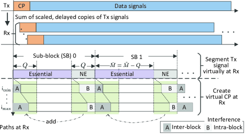
Figure 1: Illustrating the proposed virtual cyclic prefix (VCP), where $\mathsf{i}_{\mathrm{min}}$ denotes the minimum sample delay, $\mathsf{i}_{\mathrm{max}}$ the maximum, and ‘NE’ stands for ‘non-essential’. We emphasize that segmenting and adding VCP are performed on the sensing receiver side, without requiring any changes made on the OTFS transmitter.

In particular, the proposed design of adding VCP is illustrated in Fig. 1. Each sub-block is divided into two parts: the first part, consisting of $(\tilde{M}-Q)$ samples of each transmitted block, is the essential part, while the second part, consisting the remaining $Q$ samples, is the non-essential part. At the sensing receiver, a sub-block is delayed to different extent, after being reflected by different targets. From Fig. 1, we see that as long as $Q$ is no smaller than the maximum sample delay, we can add the sampled signals in the non-essential segment onto the first $Q$ samples of the essential part, and then obtain the circularly shifted versions of the signals in the essential part. Therefore, the non-essential part of each sub-block acts as a VCP. Note that $Q$ does not have to take the same value as the CP length of the underlying communication system. This is a new flexibility — the maximum range detection is not restricted by the CP length of the underlying multi-carrier communication system — as ensured by our design and not owned by many previous JCAS schemes.

Note that the practical implementation of the proposed sensing design is similar to the conventional continuous-waveform radar. As mentioned in Section II, we consider the synchronized transceiver in this paper. Thus, the receiver receives echo signals while the communication transmitter transmits OTFS signals. In practice, the segmentation parameters, i.e., $\tilde{M}$ and $Q$, can be pre-determined based on the analysis to be performed in Section V. So, within the synchronized timing frame, the receiver can segment both the original transmitted signal (as shared by the transmitter) and the echo signal, and can add VCPs for sub-blocks, as described in Fig. 1. After signal preprocessing, the receiver can then estimate target parameters using the method to be developed in Section IV.

Let $\tilde{s}_{n}[m]$ denote the essential signal part of the $n$-th transmitted sub-block. Referring to Fig. 1, we have

$$\tilde{s}_{n}[m]=s\left[n\tilde{M}+m\right],~{}m\in[0,\bar{M}-1]~{}~{}(\bar{M}=\tilde{M}-Q),$$ (9)

where $\bar{M}$ is introduced to simplify notation. After adding the proposed VCP for the $n$-th sub-block, the target echo can be rewritten based on (8), as given by

$$\tilde{x}_{n}[m]=\sum_{p=0}^{P-1}\tilde{\alpha}_{p}\tilde{s}_{n}\left[\left\langle m-l_{p}\right\rangle_{\bar{M}}\right]e^{\mathsf{j}2\pi\nu_{p}n\tilde{M}T_{\mathrm{s}}}+z^{\mathrm{A}}_{n}[m]+$$

$$~{}~{}~{}~{}~{}~{}~{}~{}~{}~{}~{}z^{\mathrm{B}}_{n}[m]+w_{n}[m],~{}m=0,1,\cdots,\bar{M}-1,$$ (10)

where $z^{\mathrm{A}}_{n}[m]$ denotes the inter-block interference for the $n$-th sub-block and $z^{\mathrm{B}}_{n}[m]$ the intra-block interference. Based on the illustration in Fig. 1, $z^{\mathrm{A}}_{n}[m]$ can be expressed as

$$z^{\mathrm{A}}_{n}[m]= \sum_{p=0}^{P-1}\tilde{\alpha}_{p}\tilde{s}_{n-1}\left[m+\tilde{M}-l_{p}\right]g_{l_{p}}[{m}]e^{\mathsf{j}2\pi\nu_{p}(n-1)\tilde{M}T_{\mathrm{s}}},$$

$$~{}~{}~{}~{}~{}~{}~{}~{}~{}~{}~{}~{}~{}~{}~{}~{}~{}~{}~{}~{}~{}~{}~{}~{}~{}m=0,1,\cdots,\mathsf{i}_{\mathrm{max}}-1,$$ (11)

and $z^{\mathrm{B}}_{n}[m]$ can be given by

$$z^{\mathrm{B}}_{n}[m]= \sum_{p=0}^{P-1}\tilde{\alpha}_{p}\tilde{s}_{n}\left[m+\bar{M}\right](1-g_{l_{p}}[m])\times$$

$$~{}~{}~{}~{}~{}~{}~{}e^{\mathsf{j}2\pi\nu_{p}n\tilde{M}T_{\mathrm{s}}},~{}m=\mathsf{i}_{\mathrm{min}},\cdots,Q-1,$$ (12)

where $g_{x}[{u}]~{}(x\leq Q-1)$ is defined as

$$g_{x}[{u}]=1,~{}\text{for }{u}\in[0,x-1];~{}g_{x}[{u}]=0\text{ for }u\in[x,Q-1].$$

Note that the two interference terms, $z^{\mathrm{A}}_{n}[m]$ and $z^{\mathrm{B}}_{n}[m]$, are the price paid for introducing VCP. Nevertheless, we notice that $z^{\mathrm{A}}_{n}[m]$ and $z^{\mathrm{B}}_{n}[m]$ can be treated as Gaussian noise uncorrelated with the essential signal part of the $n$-th sub-block. Lemma 1 provides some useful features of the different signal components in (10). Its proof is provided in Appendix -A. In addition, we point out that the impact of the two interference terms can be minimized by properly configuring $\tilde{M}$. This will be detailed in Section V.

Lemma 1

The signal components in (10), i.e., $\tilde{s}_{n}[m]$, $z^{\mathrm{A}}_{n}[m]$, $z^{\mathrm{B}}_{n}[m]$ and $w_{n}[m]$, are approximately independent over $m=0,1,\cdots,\bar{M}-1$, and are mutually uncorrelated complex centered Gaussian variables satisfying

$$\begin{gathered}\tilde{s}_{n}[m]\sim\mathcal{CN}(0,\sigma_{d}^{2}),~{}z^{\mathrm{A}}_{n}[m]\sim\mathcal{CN}(0,\sigma_{z^{\mathrm{A}}}^{2}[m]),\\ z^{\mathrm{B}}_{n}[m]\sim\mathcal{CN}(0,\sigma_{z^{\mathrm{B}}}^{2}[m]),~{}\mathrm{and}~{}w_{n}[m]\sim\mathcal{CN}(0,\sigma_{w}^{2}),\end{gathered}$$ (13)

where $\sigma_{{d}}^{2}$ is the average power of communication data $d_{i}~{}(\forall i)$, $\sigma_{z^{\mathrm{A}}}^{2}[m]$ takes the discrete values summarized in Table III-B, and the possible values of $\sigma_{z^{\mathrm{B}}}^{2}[m]$ are given in Table III-B.

TABLE I: Values of $\sigma_{z^{\mathrm{A}}}^{2}[m]$

$m$	$\left(i_{P-2},i_{P-1}\right]$	$\left(i_{P-3},i_{P-2}\right]$	$\cdots$	$\left(0,i_{0}\right]$
$\sigma_{z^{\mathrm{A}}}^{2}[m]$	$\sigma_{d}^{2}\sigma_{P-1}^{2}$	$\sigma_{d}^{2}\sum_{p=P-2}^{P-1}\sigma_{p}^{2}$	$\cdots$	$\sigma_{d}^{2}\sum_{p=0}^{P-1}\sigma_{p}^{2}$

TABLE II: Values of $\sigma_{z^{\mathrm{B}}}^{2}[m]$

$m$	$\left[i_{0},i_{1}\right)$	$\left[i_{1},i_{2}\right)$	$\cdots$	$\left[i_{P-1},Q-1\right)$
$\sigma_{z^{\mathrm{B}}}^{2}[m]$	$\sigma_{d}^{2}\sigma_{0}^{2}$	$\sigma_{d}^{2}\sum_{p=0}^{1}\sigma_{p}^{2}$	$\cdots$	$\sigma_{d}^{2}\sum_{p=0}^{P-1}\sigma_{p}^{2}$

III-C Removing Communication Information

Taking the $\bar{M}$-point DFT of $\tilde{x}_{n}[m]$ obtained in (10) w.r.t. $m$, we obtain

$${X}_{n}[l]= \sum_{p=0}^{P-1}\tilde{\alpha}_{p}\tilde{S}_{n}[l]e^{-\mathsf{j}\frac{2\pi ll_{p}}{\bar{M}}}e^{\mathsf{j}2\pi\nu_{p}n\tilde{M}T_{\mathrm{s}}}+Z_{n}^{\mathrm{A}}[l]+$$

$$~{}~{}Z_{n}^{\mathrm{B}}[l]+W_{n}[l],~{}l=0,1,\cdots,\bar{M}-1,$$ (14)

where $\tilde{S}_{n}[l]$, $Z_{n}^{\mathrm{A}}[l]$, $Z_{n}^{\mathrm{B}}[l]$ and $W_{n}[l]$ are the $\bar{M}$-point DFTs (w.r.t. $m$) of $\tilde{s}_{n}[m]$, $z^{\mathrm{A}}_{n}[m]$, $z^{\mathrm{B}}_{n}[m]$ and $w_{n}[m]$, respectively. Since $\tilde{s}_{n}[m]$ is known to the sensing receiver, $\tilde{S}_{n}[l]$ can be calculated as

$$\tilde{S}_{n}[l]=\sum_{m=0}^{\bar{M}-1}\tilde{s}_{n}[m]\mathcal{Z}_{\bar{M}}^{ml},~{}~{}\mathrm{s.t.}~{}\mathcal{Z}_{x}^{ji}=e^{-\mathsf{j}\frac{2\pi ij}{x}}\big{/}\sqrt{x},$$ (15)

where $\mathcal{Z}_{x}^{ji}$ is the $(j,i)$-th entry of an $x$-point unitary DFT matrix. As will be frequently used, the following features of the signal components in (III-C) are worth highlighting. The proof is given in Appendix -B.

Lemma 2

Given $\forall n,l$, the signal components in (III-C) satisfy

$$\begin{gathered}\tilde{S}_{n}[l]\sim\mathcal{CN}(0,\sigma_{d}^{2}),~{}W_{n}[l]\sim\mathcal{CN}(0,\sigma_{w}^{2}),\\ Z_{n}^{\mathrm{A}}[l]\sim\mathcal{CN}(0,\sigma_{Z^{\mathrm{A}}}^{2}),~{}\mathrm{and}~{}Z_{n}^{\mathrm{B}}[l]\sim\mathcal{CN}(0,\sigma_{Z^{\mathrm{B}}}^{2}),\end{gathered}$$ (16)

where each component is independent over $\forall l$. Assuming that $l_{p}~{}(\forall p)$ is uniformly distributed in $[0,Q-1]$, we then have

$$\begin{gathered}\sigma_{Z^{\mathrm{A}}}^{2}=\frac{\mathsf{i}_{\mathrm{max}}\sigma_{d}^{2}\sum_{p=0}^{P-1}(p+1)\sigma_{p}^{2}}{P\bar{M}},\\ \sigma_{Z^{\mathrm{B}}}^{2}=\frac{(Q-\mathsf{i}_{\mathrm{min}})\sigma_{d}^{2}\sum_{p=0}^{P-1}(P-p)\sigma_{p}^{2}}{P\bar{M}},\end{gathered}$$ (17)

where $\mathsf{i}_{\mathrm{max}}$ and $\mathsf{i}_{\mathrm{min}}$ are the maximum and minimum sample delay, respectively.

From (III-C), we see that communication information can be suppressed by dividing both sides of the equation by $\tilde{S}_{n}[l]$. This, however, can yield significant bursts in the resulted signal, due to the Gaussian randomness of $\tilde{S}_{n}[l]$. To reduce the bursts, we propose to use $\mathsf{k}\tilde{S}_{n}[l]$ as the divisor. The rationale of introducing $\mathsf{k}$ is: multiplying $\mathsf{k}(>1)$ can increase $\mathbb{V}\left\{\mathsf{k}\tilde{S}_{n}[l]\right\}$ and then decrease $\mathbb{C}\left\{|\mathsf{k}\tilde{S}_{n}[l]|\leq 1,~{}\forall l\right\}$. Here, $\mathbb{V}\left\{x\right\}$ denotes the variance of a random variable $x$ and $\mathbb{C}\left\{\cdot\right\}$ the event count. The following lemma helps configure $\mathsf{k}$ and its proof is given in Appendix -C.

Lemma 3

For $\mathbb{P}\left\{|\mathsf{k}\tilde{S}_{n}[l]|\leq 1\right\}=\epsilon~{}(\forall n,l)$, we can set

$$\mathsf{k}={1}\Big{/}\left({\sigma_{d}\sqrt{\ln\frac{1}{1-\epsilon}}}\right),$$ (18)

where $\epsilon$ denotes a sufficiently small probability.

Dividing both sides of (III-C) by $\mathsf{k}\tilde{S}_{n}[l]$, we obtain

$$\tilde{X}_{n}[l]=\mathbb{I}_{n}[l]\left(\sum_{p=0}^{P-1}\frac{\tilde{\alpha}_{p}}{\mathsf{k}}e^{-\mathsf{j}\frac{2\pi ll_{p}}{\bar{M}}}e^{\mathsf{j}2\pi\nu_{p}n\tilde{M}T_{\mathrm{s}}}+\tilde{Z}_{n}^{\mathrm{A}}[l]+\right.$$

$$\left.{\color[rgb]{1,1,1}\sum_{p=0}^{P}}\tilde{Z}_{n}^{\mathrm{B}}[l]+\tilde{W}_{n}[l]\right),~{}\mathbb{I}_{n}[l]=\left\{\begin{array}[]{ll}0&\text{ if }|\mathsf{k}\tilde{S}_{n}[l]|\leq 1\\ 1&\text{ otherwise }\end{array}\right.,$$ (21)

where the intermediate variables are given by

$$\begin{gathered}\tilde{Z}_{n}^{\mathrm{A}}[l]=Z^{\mathrm{A}}_{n}[l]/(\mathsf{k}\tilde{S}_{n}[l]),~{}\tilde{Z}_{n}^{\mathrm{B}}[l]=Z^{\mathrm{B}}_{n}[l]/(\mathsf{k}\tilde{S}_{n}[l]),\\ \tilde{W}_{n}[l]=W_{n}[l]/(\mathsf{k}\tilde{S}_{n}[l]).\end{gathered}$$ (22)

In case $|\mathsf{k}\tilde{S}_{n}[l]|<1$ (although unlikely given a properly selected $\mathsf{k}$), $\mathbb{I}_{n}[l]$ can help prevent noise enhancement.

We remark that the way we remove communication information is similar to the widely used OFDM sensing [18]. However, we emphasize that it is our design proposed in Sections III-A and III-B that enable OTFS sensing to be performed in such a simple manner. On the other hand, we notice that when dividing communication data symbols in OFDM sensing, the noise enhancement is not an issue in general, as PSK (with constant modulus) is assumed in most OFDM sensing works. In contrast, we are dealing with OTFS modulation that obtains the signals in the time-frequency domain through a symplectic Fourier transform; see (II), making noise enhancement issue rather severe. But thanks to the design and analysis in this section, the issue can be greatly relieved.

We also remark that the pointwise division (PWD) performed in (III-C) can be replaced by pointwise product (PWP). As PWP is performed in the frequency domain, taking the IDFT of the PWP result leads to the cyclic cross-correlation of the corresponding time-domain signals, similar to the matched filtering in conventional radar processing. The SINRs in the range-Doppler maps (RDM) generated by PWD and PWP have interesting relations, as revealed in [28]. In particular, in low SNR regions, the PWP-SINR is higher than PWD-SINR, while the relation reverses in high SNR regions. Interested readers are referred to [28] for more details.

IV Target Parameter Estimation

Enabled by the proposed pre-processing on the target echo, the resulted signal $\tilde{X}_{n}[l]$ presents a clear structure. In particular, we see from (III-C) that $e^{-\mathsf{j}\frac{2\pi ll_{p}}{\bar{M}}}$ and $e^{\mathsf{j}2\pi\nu_{p}n\tilde{M}T_{\mathrm{s}}}$ are two single-tone signals whose frequencies are related to target range and velocity, respectively. Therefore, parameter estimation in OTFS sensing is turned into estimating the center frequencies of the multi-tone signal $\tilde{X}_{n}[l]$. To fulfill the task, we develop a low-complexity and high-accuracy method, combining the commonly used estimate-and-subtract strategy [29, 30] with the frequency estimator we recently proposed in [26] for a single-tone signal. Below, we first illustrate the parameter estimation method and then analyze the computational complexity of the whole OTFS sensing scheme.

IV-A Parameter Estimation Method

The overall estimation procedure is summarized in Algorithm IV-A. In each iteration, we always estimate the parameters of the presently strongest target, as done in Steps 3) to 6) of the table; reconstruct the echo signal of the target and subtract the reconstructed echo signal, as done in Step 2); and re-perform the above three steps for the next strongest target. For ease of illustration, we assume that the $p$-th $(\forall p)$ target has stronger echo than the $p^{\prime}$-th $(\forall p^{\prime}>p)$ target, namely $|\tilde{\alpha}_{0}|>|\tilde{\alpha}_{1}|>\cdots>|\tilde{\alpha}_{P-1}|$. Thus, the signal used for estimating the $p$-th target can be given by

$$\tilde{X}_{n}^{(p)}[l]=\tilde{X}_{n}^{(p-1)}[l]-\frac{\hat{\alpha}_{p-1}}{\mathsf{k}}e^{-\mathsf{j}\frac{2\pi l\hat{l}_{p-1}}{\bar{M}}}e^{\mathsf{j}2\pi\hat{\nu}_{p-1}n\tilde{M}T_{\mathrm{s}}}$$

$$\mathrm{s.t.}~{} ~{}p\geq 1,~{}\tilde{X}_{n}^{(0)}[l]=\tilde{X}_{n}[l]\text{ given in (\ref{eq: tilde Xn[l]})},$$ (23)

where $\tilde{X}_{n}^{(p-1)}[l]$ denotes the signal used for estimating the $(p-1)$-th target, and $\hat{\alpha}_{p-1},\hat{l}_{p-1}$ and $\hat{\nu}_{p-1}$ denote the estimated parameters of the target.

Algorithm 1 Overall Parameter Estimation

Input: $\tilde{X}_{n}[l]$, as given in (III-C), and $P$ (the number of targets) 1. Initialize $p=0$; 2. Update $\tilde{X}_{n}^{(p)}[l]$ as done in (IV-A); 3. Estimate $(\tilde{l}_{p},\tilde{n}_{p})$ as done in (26); 4. Estimate $\delta_{p}$ and $\epsilon_{p}$ by running Algorithm IV-A; 5. Obtain the estimates of $l_{p}$ and $\nu_{p}$ as given in (38); 6. Estimate $\alpha_{p}$ as done in (39); 7. End if $p=P-1$; otherwise, $p=p+1$ and go to Step 2).

As mentioned earlier, $e^{-\mathsf{j}\frac{2\pi ll_{p}}{\bar{M}}}$ and $e^{\mathsf{j}2\pi\nu_{p}n\tilde{M}T_{\mathrm{s}}}$ in (III-C) are exponential signals along $l$ and $n$, respectively. Therefore, we can identify their center frequencies through a two-dimensional DFT:

$$\breve{X}_{\tilde{n}}^{(p)}[\tilde{l}]=\sum_{n=0}^{\tilde{N}-1}\sum_{l=0}^{\bar{M}-1}\tilde{X}_{n}^{(p)}[l]\mathcal{Z}_{\bar{M}}^{-l\tilde{l}}\mathcal{Z}_{\tilde{N}}^{n\tilde{n}}$$ (24)

$$=\frac{\tilde{\alpha}_{p}}{\mathsf{k}}\mathcal{S}_{\bar{M}}\left(\tilde{l}-l_{p}\right)\mathcal{S}_{\bar{N}}\left(\underbrace{\tilde{N}\tilde{M}T_{\mathrm{s}}\nu_{p}}_{n_{p}}-\tilde{n}\right)+\Xi_{\tilde{n}}^{(p)}[\tilde{l}],$$

where $\mathcal{Z}_{\bar{M}}^{-l\tilde{l}}$ and $\mathcal{Z}_{\tilde{N}}^{n\tilde{n}}$ are the DFT bases defined in (15). Note that all irrelevant terms, including interference plus noise terms given in (III-C) and the echoes of weaker targets $p^{\prime}~{}(=p+1,\cdots,P-1)$, are absorbed in $\Xi_{\tilde{n}}^{(p)}[\tilde{l}]$ for brevity. Moreover, the function $\mathcal{S}_{x}\left(y\right)$ in (24) is defined as

$$\mathcal{S}_{x}\left(y\right)=\frac{1}{\sqrt{x}}\frac{\sin\left(\frac{x}{2}\frac{2\pi y}{x}\right)}{\sin\left(\frac{1}{2}\frac{2\pi y}{x}\right)}e^{\mathsf{j}\frac{x-1}{2}\frac{2\pi y}{x}}.$$ (25)

Note that $\mathcal{S}_{x}\left(y\right)$ is a discrete sinc function which is maximized at $y=0$. Therefore, the integer parts of $(l_{p},n_{p})$ can be estimated by identifying the maximum of $\left|\breve{X}_{\tilde{n}}^{(p)}[\tilde{l}]\right|^{2}$, i.e.,

$$(\tilde{l}_{p},\tilde{n}_{p}):~{}\max{}_{\forall\tilde{l},\tilde{n}}\left|\breve{X}_{\tilde{n}}^{(p)}[\tilde{l}]\right|^{2}.$$ (26)

To obtain high-accuracy estimations of target parameters, the fractional parts of $(l_{p},n_{p})~{}\forall p$, as denoted by $(\delta_{p},\epsilon_{p})$, also need to be estimated. With reference to [26], we develop below the methods for estimating $\delta_{p}$ and $\epsilon_{p}$.

Algorithm 2 Estimating $\delta_{p}$ (or $\epsilon_{p}{}^{\dagger}$)

1) Input: $\tilde{X}_{n}^{(p)}[l]$ given in (IV-A), $(\tilde{l}_{p},\tilde{n}_{p})$ in (26) and $N_{\mathrm{iter}}$ (the maximum number of iterations); 2) Initialize: $\hat{\delta}_{p}^{(0)}=0.25d_{p}$ and $i=1$, where $d_{p}$ is given in (34); 3) Interpolate the DFT coefficients at $\tilde{l}=\tilde{l}_{p}^{\pm}\overset{\Delta}{=}\tilde{l}_{p}+\hat{\delta}_{p}^{(i-1)}\pm 0.25$, leading to $\breve{X}_{\tilde{n}_{p}}^{(p)}[\tilde{l}_{p}^{\pm}]$ given in (IV-A); 4) Construct the ratio of $\rho_{p}^{(i)}=\frac{|x_{+}|^{2}-|x_{-}|^{2}}{|x_{+}|^{2}+|x_{-}|^{2}},~{}\mathrm{s.t.}~{}x_{\pm}\overset{\Delta}{=}\breve{X}_{\tilde{n}_{p}}^{(p)}[\tilde{l}_{p}^{\pm}]$; 5) Calculate $r_{i}~{}(i=0,1,2)$ as done in (IV-A); 6) Estimate $\xi_{p}^{(i)}$ as $\hat{\xi}_{p}^{(i)}=r_{i^{*}},~{}\mathrm{s.t.}~{}i^{*}=\mathrm{argmin}{}_{i=0,1,2}~{}|r_{i}|$; 7) Update $\hat{\delta}_{p}^{(i)}=\hat{\delta}_{p}^{(i-1)}+\xi_{p}^{(i)}$; 8) Set $i=i+1$ and go back to Step 3), if $i<N_{\mathrm{iter}}$; 9) Output: the final estimate $\hat{\delta}_{p}=\hat{\delta}_{p}^{(i-1)}+\hat{\xi}_{p}^{(i)}$.

† When estimating $\epsilon_{p}$, $\delta_{p}$ above is replaced by $\epsilon_{p}$, $\xi_{p}^{(i)}$ by $\eta_{p}^{(i)}$, ${\hat{\delta}}_{p}^{(i)}$ by ${\hat{\epsilon}}_{p}^{(i)}$; see (35). Moreover, $\breve{X}_{\tilde{n}_{p}}^{(p)}[\tilde{l}_{p}^{\pm}]$ in Steps 3) and 4) becomes $\breve{X}_{\tilde{n}_{p}^{\pm}}^{(p)}[\tilde{l}_{p}]$ given in (IV-A). The remaining steps can be run without changes. However, note that $c_{1}$, $c_{3}$ and $c_{5}$ required in (IV-A) now become the Taylor coefficients of the function given in (37).

We start with $\delta_{p}$. As summarized in Algorithm IV-A, its estimation is performed iteratively. At iteration $i(\geq 1)$, we have the estimate of $\delta_{p}$ from the iteration $(i-1)$, as denoted by $\hat{\delta}_{p}^{(i-1)}$. Let $\xi_{p}^{(i)}=\delta_{p}-\hat{\delta}_{p}^{(i-1)}$ denote the estimation error which is estimated in Steps 3) to 6). In Step 3), the interpolated DFT coefficients are given by

$$\breve{X}_{\tilde{n}_{p}}^{(p)}[\tilde{l}_{p}^{\pm}]=\sum_{n=0}^{\tilde{N}-1}\sum_{l=0}^{\bar{M}-1}\tilde{X}_{n}^{(p)}[l]\mathcal{Z}_{\bar{M}}^{-l\tilde{l}_{p}^{\pm}}\mathcal{Z}_{\tilde{N}}^{n\tilde{n}_{p}}=\Xi_{\tilde{n}_{p}}^{(p)}[\tilde{l}_{p}^{\pm}]$$

$$~{}~{}~{}~{}~{}~{}~{}~{}~{}~{}~{}~{}~{}~{}~{}~{}~{}~{}~{}~{}~{}~{}~{}~{}\frac{\tilde{\alpha}_{p}}{\mathsf{k}}\mathcal{S}_{\bar{M}}\left(\tilde{l}_{p}^{\pm}-l_{p}\right)\mathcal{S}_{\bar{N}}\left(n_{p}-\tilde{n}_{p}\right),$$ (27)

where $(\tilde{l}_{p},\tilde{n}_{p})$ is obtained in (26) and $\tilde{l}_{p}^{\pm}\overset{\Delta}{=}\tilde{l}_{p}+\hat{\delta}_{p}^{(i-1)}\pm 0.25$. In Step 4), the ratio $\rho_{p}^{(i)}$ is constructed such that it can be regarded as a noisy value of the function $f(\xi_{p}^{(i)})$ given in (32). Note that the result “$\overset{(a)}{=}$” in (32) is obtained by suppressing the common terms of the numerator and denominator and by replacing $\tilde{l}_{p}^{\pm}-l_{p}$ with

$$\tilde{l}_{p}^{\pm}-l_{p}=\tilde{l}_{p}+\hat{\delta}_{p}^{(i-1)}\pm 0.25-(\tilde{l}_{p}+\delta_{p})=-\xi_{p}^{(i)}\pm 0.25.$$

Equating $f(\xi_{p}^{(i)})$ and $\rho_{p}^{(i)}$, $\xi_{p}^{(i)}$ can be estimated by solving the equation. As derived in [26], there are three roots,

$$f(\xi_{p}^{(i)})=\frac{\begin{array}[]{l}\left|\frac{\tilde{\alpha}_{p}}{\mathsf{k}}\mathcal{S}_{\bar{M}}\left(\tilde{l}_{p}^{+}-l_{p}\right)\mathcal{S}_{\bar{N}}\left(n_{p}-\tilde{n}_{p}\right)\right|^{2}\\ ~{}~{}~{}~{}~{}~{}~{}~{}~{}~{}~{}~{}~{}~{}~{}~{}~{}~{}~{}~{}~{}-\left|\frac{\tilde{\alpha}_{p}}{\mathsf{k}}\mathcal{S}_{\bar{M}}\left(\tilde{l}_{p}^{-}-l_{p}\right)\mathcal{S}_{\bar{N}}\left(n_{p}-\tilde{n}_{p}\right)\right|^{2}\end{array}}{\begin{array}[]{l}\left|\frac{\tilde{\alpha}_{p}}{\mathsf{k}}\mathcal{S}_{\bar{M}}\left(\tilde{l}_{p}^{+}-l_{p}\right)\mathcal{S}_{\bar{N}}\left(n_{p}-\tilde{n}_{p}\right)\right|^{2}\\ ~{}~{}~{}~{}~{}~{}~{}~{}~{}~{}~{}~{}~{}~{}~{}~{}~{}~{}~{}~{}~{}+\left|\frac{\tilde{\alpha}_{p}}{\mathsf{k}}\mathcal{S}_{\bar{M}}\left(\tilde{l}_{p}^{-}-l_{p}\right)\mathcal{S}_{\bar{N}}\left(n_{p}-\tilde{n}_{p}\right)\right|^{2}\end{array}}\overset{(a)}{=}\frac{\left|\mathcal{S}_{\bar{M}}\left(\xi_{p}^{(i)}-0.25\right)\right|^{2}-\left|\mathcal{S}_{\bar{M}}\left(\xi_{p}^{(i)}+0.25\right)\right|^{2}}{\left|\mathcal{S}_{\bar{M}}\left(\xi_{p}^{(i)}-0.25\right)\right|^{2}+\left|\mathcal{S}_{\bar{M}}\left(\xi_{p}^{(i)}+0.25\right)\right|^{2}}$$ (32)

$$~{}r_{1}=-k_{2}/3+2B,~{}r_{2}=-k_{2}/3-B+D,$$

$$~{}r_{3}=-k_{2}/3-B-D,$$

$$\mathrm{s.t.}~{} ~{}B=(S+T)/2,~{}D={\sqrt{3}}(S-T)\mathsf{j}/2,$$

$$~{}S=\sqrt[3]{R+\sqrt{D}},~{}T=\sqrt[3]{R-\sqrt{D}},~{}D=Q^{3}+R^{2}$$

$$~{}R={(9k_{1}k_{2}-27k_{0}-2k_{2}^{3})}/{54},~{}Q={(3k_{1}-k_{2}^{2})}/{9},$$

$$~{}k_{2}=-{\rho b_{2}}/{a_{3}},k_{1}={a_{1}}/{a_{3}},k_{0}=-{\rho}/{a_{3}},$$

$$~{}a_{1}=c_{1},a_{3}=c_{3}-{c_{1}c_{5}}\big{/}{c_{3}},b_{2}={c_{5}}\big{/}{c_{3}},$$ (33)

where $c_{1}$, $c_{3}$ and $c_{5}$ are the coefficients of the first, third and fifth power terms in the Taylor series of $f(\xi_{p}^{(i)})$ at $\xi_{p}^{(i)}=0$. Only one root provides the estimate of $\xi_{p}^{(i)}$, as determined in Step 6). Next, we update the estimate of $\delta_{p}$ in Step 7), check the stop criterion in Step 8) and, if unsatisfied, run another iteration. Above is the general iteration procedure. As for the initialization of the algorithm, $d_{p}$ is the result of the following sign test:

$$d_{p}=\mathrm{sign}\left\{\left[\breve{X}_{\tilde{n}_{p}}^{(p)}[\tilde{l}_{p}-1]-\breve{X}_{\tilde{n}_{p}}^{(p)}[\tilde{l}_{p}+1]\right]\left(\breve{X}_{\tilde{n}_{p}}^{(p)}[\tilde{l}_{p}]\right)^{*}\right\},$$ (34)

where $\breve{X}_{\tilde{n}_{p}}^{(p)}[\tilde{l}_{p}]$ is obtained by plugging $\tilde{n}=\tilde{n}_{p}$ and $\tilde{l}=\tilde{l}_{p}$ into (24) and likewise $\breve{X}_{\tilde{n}_{p}}^{(p)}[\tilde{l}_{p}\pm 1]$ is obtained. Above, the estimation steps are given with the rationales suppressed for brevity. Interested readers may refer to [26] for more details.

We notice that $\epsilon_{p}$ can also be estimated as done in Algorithm IV-A, with necessary changes pointed out in the table. For $\epsilon_{p}$, the estimation error in the iteration $i(\geq 1)$ is denoted by

$$\eta_{p}^{(i)}=\epsilon_{p}-\hat{\epsilon}_{p}^{(i-1)},$$ (35)

where $\hat{\epsilon}_{p}^{(i-1)}$ is the estimate from the previous iteration. The DFT interpolation in Step 3) now happens at $\tilde{n}=\tilde{n}_{p}^{\pm}\overset{\Delta}{=}\tilde{n}_{p}+\hat{\epsilon}_{p}^{(i-1)}\pm 0.25$ and the interpolated coefficients are given by

$$\breve{X}_{\tilde{n}_{p}^{\pm}}^{(p)}[\tilde{l}_{p}]=\sum_{n=0}^{\tilde{N}-1}\sum_{l=0}^{\bar{M}-1}\tilde{X}_{n}^{(p)}[l]\mathcal{Z}_{\bar{M}}^{-l\tilde{l}_{p}}\mathcal{Z}_{\tilde{N}}^{n\tilde{n}_{p}^{\pm}}=\Xi_{\tilde{n}_{p}^{\pm}}^{(p)}[\tilde{l}_{p}]$$

$$~{}~{}~{}~{}~{}~{}~{}~{}~{}~{}~{}~{}~{}~{}~{}~{}~{}~{}~{}~{}~{}~{}~{}~{}\frac{\tilde{\alpha}_{p}}{\mathsf{k}}\mathcal{S}_{\bar{M}}\left(\tilde{l}_{p}-l_{p}\right)\mathcal{S}_{\bar{N}}\left(n_{p}-\tilde{n}_{p}^{\pm}\right),$$ (36)

which can be likewise interpreted as $\breve{X}_{\tilde{n}_{p}}^{(p)}[\tilde{l}_{p}^{\pm}]$ given in (IV-A). Moreover, corresponding to $f(\xi_{p}^{(i)})$ given in (32), we now have

$$f(\eta_{p}^{(i)})=\frac{\left|\mathcal{S}_{\bar{N}}\left(\eta_{p}^{(i)}-0.25\right)\right|^{2}-\left|\mathcal{S}_{\bar{N}}\left(\eta_{p}^{(i)}+0.25\right)\right|^{2}}{\left|\mathcal{S}_{\bar{N}}\left(\eta_{p}^{(i)}-0.25\right)\right|^{2}+\left|\mathcal{S}_{\bar{N}}\left(\eta_{p}^{(i)}+0.25\right)\right|^{2}}$$ (37)

which is used for computing the three roots according to (IV-A).

After running Algorithm IV-A, we obtain $\hat{\delta}_{p}$ and $\hat{\epsilon}_{p}$. Adding them with $\tilde{l}_{p}$ and $\tilde{n}_{p}$ given in (26), the estimates of ${l}_{p}$ and ${\nu}_{p}$ can be written as

$$\hat{l}_{p}=\tilde{l}_{p}+\hat{\delta}_{p},~{}\hat{\nu}_{p}=(\tilde{n}_{p}+\hat{\epsilon}_{p})\Big{/}(\tilde{N}\tilde{M}T_{\mathrm{s}}),$$ (38)

where the relation between $n_{p}$ and $\nu_{p}$ is shown in (24). Substituting $\hat{l}_{p}$ and $\hat{\nu}_{p}$ into (24), the complex coefficient $\tilde{\alpha}_{p}$ can be estimated as

$$\hat{\alpha}_{p}=\mathsf{k}\breve{X}_{\tilde{n}_{p}}^{(p)}[\tilde{l}_{p}]\Big{/}\left(\mathcal{S}_{\bar{M}}\left(\tilde{l}_{p}-\hat{l}_{p}\right)\mathcal{S}_{\bar{N}}\left(\hat{n}_{p}-\tilde{n}_{p}\right)\right),$$ (39)

where the values of the two discrete sinc functions can be readily calculated based on (25).

IV-B Computational Complexity

Next, we analyze the computational complexity (CC) of the proposed OTFS and compare it with the existing methods. For pre-processing the echo, as illustrated in Section III, the only computation-intensive computations are given in (III-C) and (III-C) which perform $\tilde{N}$ numbers of $\bar{M}$-dimensional DFT and an $\tilde{N}\bar{M}$-size point-wise division, respectively. Thus, the CC of echo pre-processing is in the order of $\mathcal{O}\{\tilde{N}\bar{M}\log\bar{M}\}$. For the proposed parameter estimation method, as summarized in Algorithm IV-A, its CC is analyzed below.

• Step 3) involves a computation of a two-dimensional DFT, as done in (24), incurring the CC of $\mathcal{O}\{\tilde{N}\bar{M}\log(\bar{M}\tilde{N})\}$. Step 3) also requires $P$ times of searching for the peak in an $\tilde{N}\times\bar{M}$-dimensional range-Doppler profile, yielding the CC of $\mathcal{O}\{P\tilde{N}\log\bar{M}\}$. Since $\tilde{N}\bar{M}\log(\bar{M}\tilde{N})\gg P\tilde{N}\log\bar{M}$, the overall CC of Step 3) in Algorithm IV-A is $\mathcal{O}\{\tilde{N}\bar{M}\log(\bar{M}\tilde{N})\}$;

• Step 4) runs Algorithm IV-A for $P$ times, one for each targets. In each time, the algorithm is performed twice, one for range estimation and another for Doppler. Moreover, the CC of Algorithm IV-A is dominated by the interpolation in Step 3) [26] and is given by $\mathcal{O}\{(2N_{\mathrm{iter}}+1)\bar{M}\}$ and $\mathcal{O}\{(2N_{\mathrm{iter}}+1)\tilde{N}\}$, respectively, for range and Doppler estimations. Thus, Step 4) of Algorithm IV-A has a CC of $\mathcal{O}\{(2N_{\mathrm{iter}}+1)Px\}$ with $x=\max\{\bar{M},\tilde{N}\}$.

As will be shown in Section VI, a small value of $N_{\mathrm{iter}}$, e.g., five, can ensure a near-ML estimation performance of Algorithm IV-A. Moreover, $P$ is typically smaller than $\tilde{N}$ or $\bar{M}$ in practice. In summary, we can assert that the CC of the proposed OTFS sensing scheme is dominated by that of the two-dimensional DFT performed in Step 3) of Algorithm IV-A.

Since the ML-based OTFS sensing method [15] will be employed as a benchmark in the simulations, we provide below its CC as a comparison. As a lower bound on its CC, we only take into account the first iteration of the ML method under a single target assumption. From (22) and its context in [15], we can see that the number of range-Doppler grids is $N_{\mathrm{CP}}N$, where $N_{\mathrm{CP}}$ is the number of samples in the CP of the underlying OTFS communication system and $N$ is the size of the Doppler dimension. For each grid, the likelihood ratio given in [15, (21)] needs to be calculated, yielding the CC of $\mathcal{O}\{(MN)^{2}\}$. Thus, a lower bound of the overall CC of the ML method can be given by $\mathcal{O}\{N_{\mathrm{CP}}M^{2}N^{3}\}$. Based on (9) and the text above (7), we have $\bar{M}=\tilde{M}-Q<\tilde{M}$ and $\tilde{N}\bar{M}<\tilde{N}\bar{M}<MN$, and hence $\tilde{N}\bar{M}\log(\bar{M}\tilde{N})\ll N_{\mathrm{CP}}M^{2}N^{3}$. This demonstrates the high computational efficiency of the proposed OTFS sensing.

Before ending the section, we remark on the potential extension of the proposed method to a multiple-input and multiple-output (MIMO) system with independent signals transmitted from all antennas. Based on Remark 2, we know that the transmitted signals have low mutual cross-correlations. This suggests that we can perform the methods developed in Sections III and IV on the signal received by each receiver antenna using each transmitted signal as (3), as in a conventional orthogonal MIMO radar. However, $\tilde{x}_{n}[m]$ obtained in (10) will have an extra interference term, owing to the cross-correlations among transmitted signals. Though the interference does not affect the way the proposed methods are performed, it can degrade sensing performance. Thus, optimizing the transmitted waveforms to reduce their cross-correlations, subject to a satisfactory communication performance, can be an interesting future work.

V Optimizing Proposed Estimation Method

In this section, we optimize the proposed sensing scheme by deriving the optimal $\tilde{M}$ such that the estimation SINR is maximized. To start with, we derive the respective power expressions of the useful signal, interference and noise components in the input of the algorithm given in Algorithm IV-A; namely $\tilde{X}_{n}[l]$ given in (III-C). In doing so, we first recover the accurate signal model without neglecting the intra-symbol Doppler impact. By using the accurate signal model in (8a), in contrast to using (8b) in Section III, the signal in (10) can be rewritten as

$$\tilde{x}_{n}[m]=\sum_{p=0}^{P-1}\overbrace{\tilde{\alpha}_{p}e^{\mathsf{j}2\pi\nu_{p}n\tilde{M}T_{\mathrm{s}}}}^{\breve{\alpha}_{p}}\left(\sum_{l=0}^{\bar{M}-1}\tilde{S}_{n}[l]e^{-\mathsf{j}\frac{2\pi ll_{p}}{\bar{M}}}\mathcal{Z}_{\bar{M}}^{-lm}\right)\times$$

$$~{}~{}~{}~{}~{}~{}~{}~{}~{}~{}~{}~{}~{}~{}~{}~{}e^{\mathsf{j}2\pi\nu_{p}mT_{\mathrm{s}}}+z^{\mathrm{A}}_{n}[m]+z^{\mathrm{B}}_{n}[m]+w_{n}[m],$$ (40)

where, to account for the inter-carrier interference (ICI), the time-domain signal $\tilde{s}_{n}[\cdot]$ is replaced by its inverse IDFT, as enclosed in the round brackets. Strictly speaking, $z^{\mathrm{A}}_{n}[m]$ and $z^{\mathrm{B}}_{n}[m]$ are different from those given in (III-B) and (III-B), since $\tilde{s}_{n-1}\left[m+\tilde{M}-l_{p}\right]$ and $\tilde{s}_{n}\left[m+\bar{M}\right]$ are multiplied by extra exponential terms in a point-wise manner. The multiplication, however, changes neither the white Gaussian nature of $z^{\mathrm{A}}_{n}[m]$ and $z^{\mathrm{B}}_{n}[m]$ nor their variances. This can be validated based on Appendix -A. Thus, we continue using the same symbols here. Based on the new expression of $\tilde{x}_{n}[m]$, $\tilde{X}_{n}[l]$, as given in (III-C), can be rewritten as in (V), where the coefficient $\frac{1}{\bar{M}}$ in $\tilde{X}_{n}^{\mathrm{S}}[l]$ comes from the product of $\mathcal{Z}_{\bar{M}}^{-ml}\mathcal{Z}_{\bar{M}}^{ml}$ and the coefficient $\frac{1}{\sqrt{\bar{M}}}$ in $\tilde{X}_{n}^{\mathrm{I}}[l]$ is likewise produced. For the same reason that $z^{\mathrm{A}}_{n}[m]$ and $z^{\mathrm{B}}_{n}[m]$ are reused in (V), we continue using $Z^{\mathrm{A}}_{n}[l]$, $Z^{\mathrm{B}}_{n}[l]$ and $\tilde{W}_{n}[l]$ in (V). Next, we first derive the power expressions of the four components in (V) and then study their relations.

$$\tilde{X}_{n}[l]=\frac{\sum_{m=0}^{\bar{M}-1}\tilde{x}_{n}[m]\mathcal{Z}_{\bar{M}}^{ml}}{\mathsf{k}\tilde{S}_{n}[l]}= \underbrace{\sum_{p=0}^{P-1}\frac{\breve{\alpha}_{p}}{\mathsf{k}}e^{-\mathsf{j}\frac{2\pi ll_{p}}{\bar{M}}}\frac{1}{\bar{M}}\sum_{m=0}^{\bar{M}-1}e^{\mathsf{j}2\pi\nu_{p}mT_{\mathrm{s}}}}_{\tilde{X}_{n}^{\mathrm{S}}[l]}+\underbrace{\sum_{p=0}^{P-1}\breve{\alpha}_{p}\sum_{m=0}^{\bar{M}-1}\sum_{\begin{subarray}{c}l^{\prime}=0\\ l^{\prime}\neq l\end{subarray}}^{\bar{M}-1}\frac{\tilde{S}_{n}[l^{\prime}]}{\mathsf{k}\tilde{S}_{n}[l]}e^{-\mathsf{j}\frac{2\pi l^{\prime}l_{p}}{\bar{M}}}e^{\mathsf{j}2\pi\nu_{p}mT_{\mathrm{s}}}\frac{\mathcal{Z}_{\bar{M}}^{(l-l^{\prime})m}}{\sqrt{\bar{M}}}}_{\tilde{X}_{n}^{\mathrm{I}}[l]}$$

$$~{}~{}~{}~{}~{}~{}+\overbrace{Z^{\mathrm{A}}_{n}[l]/(\mathsf{k}\tilde{S}_{n}[l])+Z^{\mathrm{B}}_{n}[l]/(\mathsf{k}\tilde{S}_{n}[l])}^{\tilde{X}_{n}^{\mathrm{Z}}[l]}+\tilde{W}_{n}[l]$$ (41)

Some handy features that will be frequently used later are introduced first. We notice that the $p$-related summation is involved in $\tilde{X}_{n}^{\mathrm{S}}[l]$ and $\tilde{X}_{n}^{\mathrm{I}}[l]$. Lemma 4 is helpful in simplifying the calculations of their powers. We also notice that the ratio of complex Gaussian variables appears in $\tilde{X}_{n}^{\mathrm{I}}[l]$ and $\tilde{X}_{n}^{\mathrm{Z}}[l]$. The finite moments of such ratio does not exist [32]. Thus, we provide Proposition 1 to approximate the variance of the ratio. The proof of the proposition is given in Appendix -D.

Lemma 4

Let $\mathcal{X}$ denote a general expression. We have

$$\mathbb{V}\left\{\sum_{p=0}^{P-1}\alpha_{p}\mathcal{X}\right\}=\sum_{p=0}^{P-1}\sigma_{p}^{2}\mathbb{E}\left\{\mathcal{X}^{*}\mathcal{X}\right\},$$

where $\mathbb{V}\left\{x\right\}$ denotes the variance of $x$.

Proof:

As illustrated in Remark 1, we consider i.i.d. zero-mean $\alpha_{p}~{}(\forall p)$. Thus, $\mathbb{E}\left\{\sum_{p=0}^{P-1}\alpha_{p}\mathcal{X}\right\}=0$. Then, the variance can be calculated as

$$\mathbb{V}\left\{\sum_{p=0}^{P-1}\alpha_{p}\mathcal{X}\right\}=\mathbb{E}\left\{\left(\sum_{p=0}^{P-1}\alpha_{p}\mathcal{X}\right)\left(\sum_{p=0}^{P-1}\alpha_{p}\mathcal{X}\right)^{*}\right\}$$

$$=\sum_{p=0}^{P-1}\sigma_{p}^{2}\mathbb{E}\left\{\mathcal{X}^{*}\mathcal{X}\right\},$$ (42)

where the cross-terms are suppressed due to $\mathbb{E}\left\{\alpha_{p_{1}}\alpha_{p_{2}}^{*}\right\}=0$ given $\forall p_{1}\neq p_{2}$. ∎

Proposition 1

Let $x\sim\mathcal{CN}(0,\sigma_{x}^{2})$ and $y\sim\mathcal{CN}(0,\sigma_{y}^{2})$ denote two uncorrelated complex Gaussian variables. Defining $z=\frac{x}{y}$, we have $\mathbb{E}\left\{z\right\}=0$. Provided that $\mathbb{P}\left\{|y|\leq 1\right\}=\epsilon$, $\sigma_{x}^{2}\ll\sigma_{y}^{2}$ and $\rho=\sigma_{x}^{2}/\sigma_{y}^{2}$, the variance of $z$ can be approximated by

$$\sigma_{z}^{2}\approx\mathsf{b}(\epsilon)\rho,~{}\mathrm{s.t.}~{}\mathsf{b}(\epsilon)=2\left(\ln\left(\frac{2(1-\epsilon)}{\sqrt{\epsilon(2-\epsilon)}}\right)-1\right).$$ (43)

V-A Power Expressions

Power of $\tilde{X}_{n}^{\mathrm{S}}[l]$: Applying Lemma 4, the variance of $\tilde{X}_{n}^{\mathrm{S}}[l]$ given in (V), as denoted by $\sigma_{\mathrm{S}}^{2}$, can be calculated as

$$\sigma_{\mathrm{S}}^{2}=\frac{1}{\mathsf{k}^{2}\bar{M}^{2}}\underbrace{\sum_{p=0}^{P-1}\sigma_{p}^{2}\mathbb{E}\left\{\begin{array}[]{l}\left(\sum_{m_{1}=0}^{\bar{M}-1}e^{\mathsf{j}2\pi\nu_{p}m_{1}T_{\mathrm{s}}}\right)\\ ~{}~{}~{}~{}~{}\times\left(\sum_{m_{2}=0}^{\bar{M}-1}e^{-\mathsf{j}2\pi\nu_{p}m_{2}T_{\mathrm{s}}}\right)\end{array}\right\}}_{\Pi}$$ (46)

$$\approx\frac{1}{\mathsf{k}^{2}}\Big{(}\sigma_{P}^{2}+\mathsf{a}-\mathsf{a}\bar{M}^{2}\Big{)},$$

$$\mathrm{s.t.}~{}\mathsf{a}=\frac{\pi^{2}T_{\mathrm{s}}^{2}}{3}\sum_{p=0}^{P-1}\sigma_{p}^{2}\nu_{p}^{2},~{}\sigma_{P}^{2}=\sum_{p=0}^{P-1}\sigma_{p}^{2}$$ (47)

where the approximation is due to the Taylor series used for calculating $\Pi$, as illustrated in Appendix -E.

Power of $\tilde{X}_{n}^{\mathrm{I}}[l]$: Applying Lemma 4, the variance of $\tilde{X}_{n}^{\mathrm{I}}[l]$ given in (V), as denoted by $\sigma_{\mathrm{I}}^{2}$, can be calculated as

$$\sigma_{\mathrm{I}}^{2}=\mathbb{E}\left\{\left|\frac{\tilde{S}_{n}[l^{\prime}]}{\mathsf{k}\tilde{S}_{n}[l]}\right|^{2}\right\}\times$$

$$\underbrace{\sum_{p=0}^{P-1}\sigma_{p}^{2}\mathbb{E}\left\{\begin{array}[]{l}\sum_{{l^{\prime}=0,l^{\prime}\neq l}}^{\bar{M}-1}\left(\sum_{m_{1}=0}^{\bar{M}-1}e^{\mathsf{j}2\pi\nu_{p}m_{1}T_{\mathrm{s}}}\frac{\mathcal{Z}_{\bar{M}}^{(l-l^{\prime})m_{1}}}{\sqrt{\bar{M}}}\right)\\ ~{}~{}~{}~{}~{}\times\left(\sum_{m_{2}=0}^{\bar{M}-1}e^{-\mathsf{j}2\pi\nu_{p}m_{2}T_{\mathrm{s}}}\frac{\mathcal{Z}_{\bar{M}}^{-(l-l^{\prime})m_{2}}}{\sqrt{\bar{M}}}\right)\end{array}\right\}}_{\Gamma},$$ (50)

$$={{\mathsf{b}(\epsilon)\mathsf{k}^{-2}}(\mathsf{a}\bar{M}^{2}-\mathsf{a})},~{}\mathrm{s.t.}~{}\mathsf{a}=\frac{\pi^{2}T_{\mathrm{s}}^{2}}{3}\sum_{p=0}^{P-1}\sigma_{p}^{2}\nu_{p}^{2}$$ (51)

where $\mathbb{E}\left\{\left|\frac{\tilde{S}_{n}[l^{\prime}]}{\mathsf{k}\tilde{S}_{n}[l]}\right|^{2}\right\}=\mathsf{b}(\epsilon)\mathsf{k}^{-2}$ according to Lemma 2 and Proposition 1, and $\Gamma$ is calculated in (54) (at the top of next page).

$$\Gamma=\sum_{p=0}^{P-1}\sigma_{p}^{2}\sum_{{l^{\prime}=0,l^{\prime}\neq l}}^{\bar{M}-1}\sum_{m_{1}=0}^{\bar{M}-1}\sum_{m_{2}=0}^{\bar{M}-1}e^{\mathsf{j}2\pi\nu_{p}(m_{1}-m_{2})T_{\mathrm{s}}}\frac{\mathcal{Z}_{\bar{M}}^{(l-l^{\prime})(m_{1}-m_{2})}}{\bar{M}^{\frac{3}{2}}}\overset{(a)}{=}\underbrace{\sum_{p=0}^{P-1}\sigma_{p}^{2}{\left(\begin{array}[]{l}\sum_{{l^{\prime}=0}}^{\bar{M}-1}\sum_{m_{1}=0}^{\bar{M}-1}\sum_{m_{2}=0}^{\bar{M}-1}\\[2.84526pt] ~{}~{}e^{\mathsf{j}2\pi\nu_{p}(m_{1}-m_{2})T_{\mathrm{s}}}\frac{\mathcal{Z}_{\bar{M}}^{(l-l^{\prime})(m_{1}-m_{2})}}{\bar{M}^{\frac{3}{2}}}\end{array}\right)}}_{\Gamma_{1}}$$ (54)

$$~{}~{}~{}~{}~{}~{}~{}~{}~{}~{}-\underbrace{\sum_{p=0}^{P-1}\sigma_{p}^{2}\left(\begin{array}[]{l}\sum_{{l^{\prime}=l}}\sum_{m_{1}=0}^{\bar{M}-1}\sum_{m_{2}=0}^{\bar{M}-1}\\[2.84526pt] ~{}~{}e^{\mathsf{j}2\pi\nu_{p}(m_{1}-m_{2})T_{\mathrm{s}}}\frac{\mathcal{Z}_{\bar{M}}^{0\times(m_{1}-m_{2})}}{\bar{M}^{\frac{3}{2}}}\end{array}\right)}_{{\Pi}/{\bar{M}^{2}}}\overset{(b)}{=}\sigma_{P}^{2}-\Big{(}\sigma_{P}^{2}+\mathsf{a}-\mathsf{a}\bar{M}^{2}\Big{)}=\mathsf{a}\bar{M}^{2}-\mathsf{a}.$$ (57)

In the calculation, the result $\overset{(a)}{=}$ is obtained by separately considering the summation over $l^{\prime}=0,1,\cdots,\bar{M}-1$ (leading to $\Gamma_{1}$) and the special case of $l^{\prime}=l$ (which happens to become $\Pi/\bar{M}^{2}$). As calculated in Appendix -F, $\Gamma_{1}=\sigma_{P}^{2}$. Then, combining the result of $\Pi$ calculated in Appendix -E, we obtain the result $\overset{(b)}{=}$ in (54).

Power of $\tilde{X}_{n}^{\mathrm{Z}}[l]$: According to Lemma 2, $Z^{\mathrm{A}}_{n}[l]$, $Z^{\mathrm{B}}_{n}[l]$ and $\tilde{S}_{n}[l]$ are zero-mean complex Gaussian variables. Thus, applying Lemma 1, we have

$$\mathbb{V}\left\{\frac{Z^{\mathrm{A}}_{n}[l]}{\mathsf{k}\tilde{S}_{n}[l]}\right\}= \mathbb{E}\left\{\left|\frac{Z^{\mathrm{A}}_{n}[l]}{\mathsf{k}\tilde{S}_{n}[l]}\right|^{2}\right\}=\frac{\mathsf{b}(\epsilon)\sigma_{Z^{\mathrm{A}}}^{2}}{\mathsf{k}^{2}\sigma_{d}^{2}}$$

$$= \frac{\mathsf{b}(\epsilon)\mathsf{k}^{-2}\mathsf{i}_{\mathrm{max}}\sum_{p=0}^{P-1}(p+1)\sigma_{p}^{2}}{P\bar{M}},$$

where $\sigma_{Z^{\mathrm{A}}}^{2}$ is given in (17). Likewise, we obtain

$$\mathbb{V}\left\{\frac{Z^{\mathrm{B}}_{n}[l]}{\mathsf{k}\tilde{S}_{n}[l]}\right\}=\frac{\mathsf{b}(\epsilon)\mathsf{k}^{-2}(Q-\mathsf{i}_{\mathrm{min}})\sum_{p=0}^{P-1}(P-p)\sigma_{p}^{2}}{P\bar{M}}.$$

Using the above two results, the variance of $\tilde{X}_{n}^{\mathrm{Z}}[l]$ given in (V), as denoted by $\sigma_{\mathrm{Z}}^{2}$, can be calculated as

$$\sigma_{Z}^{2}=\mathbb{V}\left\{\frac{Z^{\mathrm{A}}_{n}[l]}{\mathsf{k}\tilde{S}_{n}[l]}\right\}+\mathbb{V}\left\{\frac{Z^{\mathrm{B}}_{n}[l]}{\mathsf{k}\tilde{S}_{n}[l]}\right\}+$$

$$~{}~{}~{}~{}~{}~{}~{}~{}\mathbb{E}\left\{\left(\frac{Z^{\mathrm{A}}_{n}[l]}{\mathsf{k}\tilde{S}_{n}[l]}\right)^{*}\frac{Z^{\mathrm{B}}_{n}[l]}{\mathsf{k}\tilde{S}_{n}[l]}\right\}+\mathbb{E}\left\{\left(\frac{Z^{\mathrm{B}}_{n}[l]}{\mathsf{k}\tilde{S}_{n}[l]}\right)^{*}\frac{Z^{\mathrm{A}}_{n}[l]}{\mathsf{k}\tilde{S}_{n}[l]}\right\}$$

$$\approx\frac{\mathsf{b}(\epsilon)\left(\begin{array}[]{l}\mathsf{i}_{\mathrm{max}}\sum_{p=0}^{P-1}(p+1)\sigma_{p}^{2}\\ ~{}~{}~{}~{}~{}~{}~{}~{}~{}+(Q-\mathsf{i}_{\mathrm{min}})\sum_{p=0}^{P-1}(P-p)\sigma_{p}^{2}\end{array}\right)}{\mathsf{k}^{2}P\bar{M}}$$ (60)

$$\overset{\begin{subarray}{c}\mathsf{i}_{\mathrm{min}}=0\\ \mathsf{i}_{\mathrm{max}}=Q\end{subarray}}{\leq}~{}~{}\frac{\mathsf{b}(\epsilon)Q(P+1)\sigma_{P}^{2}}{\mathsf{k}^{2}P\bar{M}},~{}\mathrm{s.t.}~{}\sigma_{P}^{2}=\sum_{p=0}^{P-1}\sigma_{p}^{2},$$ (61)

where the two expectations are approximately zeros, as proved in Appendix -G. The equality in the last line can be achieved when the two conditions are satisfied, $\mathsf{i}_{\mathrm{min}}=0$ and $\mathsf{i}_{\mathrm{max}}=Q$. These conditions are likely to hold for a large $P$, since the larger $P$ is, the more variety can present among targets.

Power of $\tilde{W}_{n}[l]$: According to (III-C), we have $\tilde{W}_{n}[l]=W_{n}[l]/(\mathsf{k}\tilde{S}_{n}[l])$ which is the ratio of two complex Gaussian. Thus, directly applying Proposition 1 gives us

$$\sigma_{W}^{2}=\mathbb{V}\left\{\tilde{W}_{n}[l]\right\}=\frac{\mathsf{b}(\epsilon)\sigma_{w}^{2}}{\mathsf{k}^{2}\sigma_{d}^{2}},$$ (62)

where $\mathbb{V}\left\{W_{n}[l]\right\}=\sigma_{w}^{2}$, as proved in Lemma 2.

V-B Maximizing SINR for Parameter Estimation

With the power of individual signal components in ${\tilde{X}_{n}[l]}$ derived, we proceed to analyze the overall SINR for the proposed parameter estimation method and derive the optimal $\tilde{M}$. Note that a two-dimensional DFT along $n$ and $l$ is taken for ${\tilde{X}_{n}[l]}$ before estimating target parameters; see Algorithm IV-A. The maximum SINR improvement brought by the DFT is $\bar{M}\tilde{N}$; see (24). This is because $\tilde{X}_{n}^{\mathrm{S}}[l]$ is coherently accumulated with the maximum amplitude gain of $\bar{M}\tilde{N}$, while $\tilde{X}_{n}^{\mathrm{I}}[l]$ and $\tilde{X}_{n}^{\mathrm{Z}}[l]$ are only incoherently accumulated with the power gain of $\bar{M}\tilde{N}$. With the SINR gain of $\bar{M}\tilde{N}$ taken into account, the overall SINR for parameter estimation can be given by

$$\gamma=\frac{f(\bar{M})}{g(\bar{M})}\overset{\Delta}{=}\frac{\bar{M}\tilde{N}\sigma_{\mathrm{S}}^{2}}{\sigma_{\mathrm{I}}^{2}+\sigma_{{Z}}^{2}+\sigma_{{W}}^{2}},$$ (63)

where $\sigma_{\mathrm{S}}^{2}$, $\sigma_{\mathrm{I}}^{2}$, $\sigma_{Z}^{2}$ and $\sigma_{W}^{2}$ are derived in (46), (V-A), (V-A) and (62), respectively. To avoid overly cumbersome expressions, we denote the numerator and denominator as different function of $\bar{M}$ and study their monotonic features separately. In particular, the following interesting results are achieved, with the proof given in Appendices -H and -I.

Proposition 2

The numerator function $f(\bar{M})$ in (63) is concave w.r.t. $\bar{M}$. Given $\bar{M}\gg 3Q/2$, $f(\bar{M})$ is maximized at

$$\bar{M}=\bar{M}_{f}^{*}\approx\sqrt[3]{{(Q\mathsf{a}+Q\sigma_{P}^{2})}\big{/}{(2\mathsf{a})}}.$$

Proposition 3

The denominator function $g(\bar{M})$ in (63) is convex w.r.t. $\bar{M}$ and is minimized at

$$\bar{M}=\bar{M}_{g}^{*}=\sqrt[3]{{(Q(P+1)\sigma_{P}^{2})}\big{/}{(2\mathsf{a}P)}}.$$

From the two propositions, $f(\bar{M})$ and $g(\bar{M})$ seem to achieve the extremum at different values of $\bar{M}$. Nevertheless, taking into account the practical values of the variables in their respective expressions, we have the following result.

Corollary 1

The optimal $\bar{M}$ for the numerator and denominator functions in (63) satisfy $\bar{M}_{f}^{*}\approx\bar{M}_{g}^{*}\approxeq\sqrt[3]{{Q\sigma_{P}^{2}}\big{/}{(2\mathsf{a})}}$, where the equality can be approached as $P$ becomes larger.

Proof:

As defined in (46), $\mathsf{a}=\frac{\pi^{2}T_{\mathrm{s}}^{2}}{3}\sum_{p=0}^{P-1}\sigma_{p}^{2}\nu_{p}^{2}$. Thus we have the following upper bound of $2\mathsf{a}$

$$2\mathsf{a}=\frac{\pi^{2}T_{\mathrm{s}}^{2}}{3}\sum_{p=0}^{P-1}2\sigma_{p}^{2}\nu_{p}^{2}\leq\frac{\pi^{2}T_{\mathrm{s}}^{2}}{3}\sum_{p=0}^{P-1}(\sigma_{p}^{2}+\nu_{p}^{2}).$$

Applying the above inequality, we have

$$Q\sigma_{P}^{2}/(2\mathsf{a})\geq\frac{Q}{\frac{\pi^{2}T_{\mathrm{s}}^{2}}{3}(1+\frac{1}{\sigma_{P}^{2}}\sum_{p=0}^{P-1}\nu_{p}^{2})}\gg Q/2$$

where the last result is because $T_{\mathrm{s}}$ can be in the order of $10^{-6}$ while $\nu_{p}$ is only in the order of $10^{3}$. Reflecting the above relation in Proposition 2, we obtain $\bar{M}_{f}^{*}\approx\sqrt[3]{{Q\sigma_{P}^{2}}\big{/}{(2\mathsf{a})}}$. Given a large $P$, $\bar{M}_{g}^{*}$ derive in Proposition 3 becomes $\bar{M}_{g}^{*}\approxeq\sqrt[3]{{Q\sigma_{P}^{2}}\big{/}{(2\mathsf{a})}}\approx\bar{M}_{f}^{*}$. ∎

In summary, we highlight below the key features of the proposed OTFS sensing methods. First, the actual range and Doppler dimensions, as denoted by $\tilde{M}$ and $\tilde{N}$, respectively, are not limited to the original dimensions of the underlying OTFS system, i.e., $M$ and $N$. Second, the maximum range that can be estimated by the proposed design is not subject to the CP length of the OTFS system and can be flexibly adjusted by changing $Q$, i.e., the length of the proposed VCP. Third, the SINR for target parameter estimation can be maximized by setting

$$\tilde{M}=\sqrt[3]{\frac{Q\sigma_{P}^{2}}{(2\mathsf{a})}}+Q,~{}\tilde{N}=\left\lfloor\frac{MN}{\tilde{M}}\right\rceil$$ (64)

where $\mathsf{a}$ and $\sigma_{P}^{2}$ are defined in (46). Note that the relation $\tilde{M}=\bar{M}+Q$, as given in (9), is used above. Also note that the optimization in this section has included the potential ICI caused by the intra-sub-block Doppler impact. Thus, even if a large $Q$ results in a large $\tilde{M}$ according to (64), the optimal $\tilde{M}$ is guaranteed to maximizes the sensing SINR, whether ICI is present or not.

VI Simulation Results

In this section, simulation results are provided to validate the proposed designs and analyses.

VI-A Comparison with Benchmark Method

In a first set of simulations, we compare the proposed design with the state-of-the-art OTFS sensing method [15] which performs the maximum likelihood (ML) estimation. In short, the ML method [15] first transforms $x[i]$ given in (III) into the delay-Doppler domain by performing an inverse symplectic Fourier transform, i.e., the inverse transform of that performed in (II). The result is stacked into an $I$-dimensional $(I=MN)$ column vector, as denoted by $\mathbf{y}_{\mathrm{ML}}$. Then a multi-layer two-dimensional searching is carried out, using the coefficients $\mathbf{H}_{\mathrm{ML}}^{a}(l_{g}^{a},\nu_{g}^{a})\mathbf{d}$, where $\mathbf{d}$ is obtained by stacking $d_{kM+l}$ into an $I$-dimensional column vector ($k$ first) and $\mathbf{H}_{\mathrm{ML}}^{a}(l_{g}^{a},\nu_{g}^{a})$ is the input-output response matrix at a delay-Doppler grid $(l_{g}^{a},\nu_{g}^{a})$; refer to [15, Eq. (15)] for its detailed expression. The superscript $()^{a}$ denotes the layer index and the subscript $()_{g}$ denotes the grid index. For a single target, the 2D searching can be depicted as follows,

$$(\hat{l}^{a},\hat{\nu}^{a}):~{}\max_{(l_{g}^{a},\nu_{g}^{a})\in\mathcal{S}_{a}}\frac{\left(\mathbf{H}_{\mathrm{ML}}^{a}(l_{g}^{a},\nu_{g}^{a})\mathbf{d}\right)^{\mathrm{H}}\mathbf{y}_{\mathrm{ML}}}{\left(\left(\mathbf{H}_{\mathrm{ML}}^{a}(l_{g}^{a},\nu_{g}^{a})\mathbf{d}\right)^{\mathrm{H}}\left(\mathbf{H}_{\mathrm{ML}}^{a}(l_{g}^{a},\nu_{g}^{a})\mathbf{d}\right)\right)},$$ (65)

where $(\hat{l}^{a},\hat{\nu}^{a})$ is the pair of estimated parameters and $\mathcal{S}_{a}$ is the delay-Doppler region to be searched at layer $a$.

For simulation efficiency, we take ${l}_{g}^{a}=l^{a}~{}(\forall a,g)$, where $l^{a}$ is the true value of sample delay at layer $a$. Thus, we only perform ML estimation for the target velocity. Moreover, we set the number of grids in each layer as five, i.e., $|\mathcal{S}_{a}|=5$, and the total number of layers as eight, i.e., $a=0,1,\cdots,7$. More specifically, at $a=0$, we set $\nu_{g}^{0}=g\Delta_{f}/4~{}(g=0,1,2,3,4)$. Note that $\Delta_{f}$, the sub-carrier interval, is also the unambiguously measurable region of the Doppler frequency for the ML method [15]. For $a\geq 1$, the searching region of layer $a$ is reduced to $\Delta_{f}/4^{a}$ centered at $\hat{\nu}^{a-1}$. In addition, we set a rule that stops the iterative searching at layer $a$ if $\hat{\nu}_{g}^{a}\neq{\nu}^{a}$ and take ${\nu}^{a}$ as the final velocity estimate, where ${\nu}^{a}$ is the true value. For fair comparison with the ML method [15], the key system parameters set therein are used here only with minor modification. The settings are summarized in Table VI-A.

TABLE III: Simulation Parameters

Variable	Description	Value
$f_{\mathrm{c}}$	Carrier frequency	$5.89$ GHz
$B$	Bandwidth	$10$ MHz
$\Delta_{f}$	Sub-carrier interval	$B/M$ MHz
$M$	No. of sub-carriers per symbol	$25$
$N$	No. of symbols	$40$
$\sigma_{d}^{2}$	Power of data symbol $d_{kM+l}$ give in (II)	$0$ dB
$\sigma_{0}^{2}$	Power of $\alpha_{p}~{}(p=0)$; see (8)	$0$ dB
$\sigma_{w}^{2}$	Variance of AWGN $w_{n}[m]$ given in (8)	$-10:2:10$ dB
$r$	Target range	$30$ m
$v$	Target velocity	$80$ km/h
$N_{\mathrm{iter}}$	No. of iteration for Algorithm IV-A	5

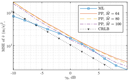
Figure 2: MSE of velocity estimation, denoted by $\hat{v}$, versus $\gamma_{0}(=\sigma_{0}^{2}/\sigma_{w}^{2})$, i.e., the SNR of $x_{n}[m]$ given in (8), where $ML$ is for the benchmark method [15] and PP for the proposed design.

Fig. 2 plots the mean squared error (MSE) of the velocity estimation, denoted by $\hat{v}$, against the SNR, denoted by $\gamma_{0}$. Here, $\gamma_{0}=(\sigma_{0}^{2}/\sigma_{w}^{2})$ is defined based on the sensing-received signal in the time domain, i.e., $x_{n}[m]$ given in (8). We see that, in overall, the proposed method has a comparable performance to the ML method [15]. Interestingly, we see different performance relation between the two methods in three SNR regions.

1. As $\gamma_{0}$ increases from $-10$ dB to $-2$ dB, the ML outperforms the proposed method, with the performance gap becoming increasingly smaller. This is because the proposed estimation algorithm, as summarized in Algorithm IV-A, can return any value in $[0,\frac{1}{\tilde{M}T_{\mathrm{s}}}]$, in the presence of strong noises. In contrast, the way the ML method is simulated makes its velocity estimation error bounded to $80/3.6$;

2. For $\gamma_{0}\in[-1,5]$ dB, the proposed method is able to outperform the ML method. The reason is that the proposed method provides off-grid estimations, while the ML method performs on-grid searching; and

3. As $\gamma_{0}$ increases over $5$ dB, an increasing (yet small) performance gap between the proposed and the ML methods can be seen. The slight degrading of the proposed method is caused by the interference introduced during adding VCP; refer to Fig. 1. In particular, when the noise power keep decreasing, the impact of the inter- and intra-symbol interference becomes gradually dominant.

Nevertheless, we see from Fig. 2 that increasing $\tilde{M}$ can help reduce the impact of the interference. This is expected. Based on the parameter setting in Table VI-A and Corollary 1, we have $\bar{M}_{f}^{*}\approx\bar{M}_{g}^{*}\approxeq 247.8675$. According to Propositions 2 and 3, the estimation SINR increases with $\tilde{M}$ when $\tilde{M}\leq\bar{M}_{f}^{*}$. That is, a larger $\tilde{M}$ corresponds to a more accurate $\hat{v}$ estimation.

Fig. 2 also plots the CLRB of velocity estimation to validate the high accuracy of the parameter estimation methods developed in Section IV. As derived Appendix -J, the CRLB is given by

$$\mathrm{CRLB}\{\hat{v}\}=\frac{\lambda^{2}}{4}\frac{1}{(\tilde{M}\tilde{N}T_{\mathrm{s}})^{2}}\frac{6}{4\pi^{4}\tilde{N}\bar{M}\gamma_{0}/\mathsf{b}(\epsilon)},$$ (66)

where $\mathsf{b}(\epsilon)$ is given in Proposition 1. We see from Fig. 2 that the asymptotic performance of our estimation is slightly worse than the ML estimation. This owes to the interference introduced when adding VCP. Note that the low-SNR performance of the ML method is not accurate in Fig. 2. As explained above, this is because the way we simulate the method bounds estimation error.

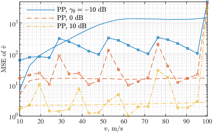
Figure 3: MSE of $\hat{v}$ versus $v$, where $\tilde{M}=100$ is taken for the proposed method (PP) and the curves with markers correspond to the ML method [15].

Fig. 3 plots the MSE of $\hat{v}$ versus different values of $v$. We see that the proposed method can achieve a comparable performance to the ML method [15] at a moderately high or high SNRs. We also see that the proposed method presents an even performance over a large region of $v$, while the good performance of the ML method can be velocity-selective. From Figs. 2 and 3, we conclude that the proposed method can provide an ML-like estimation performance for OTFS-based sensing.

VI-B Wide Applicability of Proposed Methods

Next, we validate the analysis of the impact of $\tilde{M}$ on the proposed OTFS sensing framework. To also show the wide applicability of the proposed method, we employ another set of system parameters, as summarized in Table VI-B, where $\mathcal{U}_{[a,b]}$ denotes the uniform distribution in $[a,b]$. Note that $P=4$ means four targets are set. Also note that the Doppler frequency of $4.63$ KHz corresponds to the maximum target velocity of $500$ km/h.

TABLE IV: Simulation Parameters

Variable	Value	Variable	Value	Variable	Value
$f_{\mathrm{c}}$	$5$ GHz	$B$	$12$ MHz	$P$	$4$
$M$	$400$	$N$	$100$	$l_{p}~{}(\forall p)$	$\mathcal{U}_{[0,Q-1]}$
$\sigma_{w}^{2}$	$-10$ dB	$\sigma_{d}^{2}$	$0$ dB	$\sigma_{p}~{}(\forall p)$	$0$ dB
$\sigma_{0}^{2}$	$0$ dB	$\nu_{p}~{}(\forall p)$	$\mathcal{U}_{[-4.63~{}\mathrm{KHz},4.63~{}\mathrm{KHz}]}$

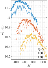
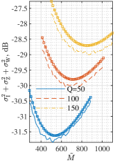
Figure 4: Illustrating the impact of $\tilde{M}$ on the powers of signal and other components, as derived in Section V-A, where the curves with markers are theoretical results while the ones without markers are simulated.

Fig. 4 illustrates the impact of $\tilde{M}$ on the powers of the signal and other components in $\tilde{X}_{n}[l]$ given in (V), where the power expressions of $\sigma_{\mathrm{S}}^{2}$, $\sigma_{\mathrm{I}}^{2}$, $\sigma_{Z}^{2}$ and $\sigma_{W}^{2}$, as derived in (46), (V-A), (V-A) and (62), respectively, are plotted as the theoretical references. From Fig. 4, we see that the derived expressions can precisely depict the actual powers of different signal components. We also see from the left sub-figure that the signal power presents an approximate concave relation with $\tilde{M}$, as proved in Proposition 2. Moreover, we see from the right sub-figure that the overall power of interference plus noises is indeed a convex function of $\tilde{M}$, which validates Proposition 3. In addition, jointly comparing the two sub-figures, we can see that the extrema of $\sigma_{\mathrm{S}}^{2}$ and $(\sigma_{\mathrm{I}}^{2}+\sigma_{\mathrm{Z}}^{2}+\sigma_{\mathrm{W}}^{2})$ are achieved at approximately identical $\tilde{M}$ for each value of $Q$. This confirms the analysis in Corollary 1.

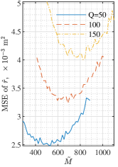
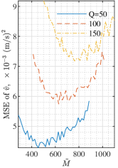
Figure 5: MSE of parameter estimations versus $\tilde{M}$, where the mean is calculated over the squared estimation errors of all the four targets.

Fig. 5 plots the MSE of range and velocity estimations against $\tilde{M}$. We see that, as consistent with the SINR variations reflected in Fig. 4, the MSEs of the estimations of both parameters are convex functions of $\tilde{M}$ and are minimized at the optimal $\tilde{M}$ derived in Corollary 1. We also see that the proposed method achieves the high-accuracy estimations of the ranges and velocities of all four targets (as the MSE is calculated over the squared estimation errors of all targets). Moreover, we see from Fig. 4 that $Q$ also has a non-trivial impact on OTFS sensing performance. In particular, as $Q$ becomes larger, the whole MSE curve shifts upwards. This is because a larger $Q$ leads to a smaller number of samples in the essential part of each sub-block; see Fig. 1; as a further result, the coherent accumulation gain of the two-dimensional DFT performed in (24) for parameter estimation is also reduced.

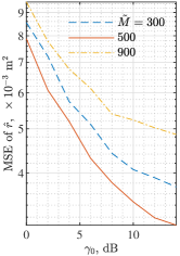
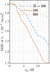
Figure 6: MSE of parameter estimations versus $\gamma_{0}$, where $Q=50$ and the mean is calculated over the squared estimation errors of all the four targets.

Fig. 6 illustrates the MSE of parameter estimations against $\gamma_{0}$. Based on Fig. 4, we see that the optimal $\tilde{M}$ is about $500$. Thus, we take three values of $\tilde{M}$ in this simulation to further illustrate the impact of $\tilde{M}$ under different $\gamma_{0}$. As consistent with Fig. 4 and 5, the best MSE performance versus $\gamma_{0}$ is achieved at $\tilde{M}=500$. Moreover, we also see that the MSE performance under $\tilde{M}=500$ is better than that under $\tilde{M}=900$. This is also consistent with what observed in Fig. 5. In addition, we see that the impact of $\tilde{M}$ is more prominent at a higher SNR. This is because as noise becomes weaker, the interference component has a more dominating effect, which also makes the impact of $\tilde{M}$ more obvious.

VII Conclusions and Remarks

To advocate OTFS-based JCAS for future IIoT as an ultra-reliable, low-latency and high-accuracy communication and sensing solution, we develop in this paper a low-complexity OTFS sensing method with the near-ML performance. This is achieved by a series of waveform pre-processing which addresses the challenges of ICI and ISI, and successfully removes the the impact of communication data symbols in the time-frequency domain without amplifying noises. This is also accomplished by a high-accuracy and off-grid method for estimating range of velocity. The complexity of the method is only dominated by a two-dimensional DFT. This is further attained by the comprehensive analysis of SINR for parameter estimation and the optimization of a key parameter in the proposed method. Extensive simulations are provided, validating the near-ML performance and wide applicability of our method as well as the precision of our SINR analysis.

We remark that additional research effort would be necessary to make OTFS-based JCAS more ready for IIoT applications. First, sensing between the distributed, non-coherent, asynchronous transmitter and receiver is yet to be solved, where the estimation ambiguities caused by timing and frequency offset are challenging to remove [7]. Second, networked sensing can combine the capabilities and diversities of different IIoT nodes for better performance, which is yet largely unexplored. Third, using sensing results to assist communications can further enhance the energy-efficiency of JCAS. A recent work [16] shows the benefit of doing so in the vehicular network. More studies are necessary to account for the unique needs/features of IIoT applications. Fourth, in the spirit of JCAS, we may be able to make changes to the transmitted OTFS signal, e.g., inserting more CPs as in OFDM systems. This, however, requires a holistic evaluation on the trade-off between the performance loss of communications and performance gain of sensing. The state-of-the-art OFDM-based JCAS waveform design [33, 34, 35, 36, 37] can provide good references for future OTFS JCAS designs.

-A Proof of Lemma 1

$$\sigma_{z^{\mathrm{A}}}^{2}[m]=\mathbb{E}\left\{\left|z^{\mathrm{A}}_{n}[m]\right|^{2}\right\}=\mathbb{E}\left\{\left(\sum_{p_{1}=0}^{P-1}\tilde{\alpha}_{p_{1}}^{*}\tilde{s}_{n-1}^{*}\left[m+\tilde{M}-i_{p_{1}}\right]g_{i_{p_{1}}}[{m}]e^{-\mathsf{j}2\pi\nu_{p_{1}}(n-1)\tilde{M}T_{\mathrm{s}}}\right)\times\left(\sum_{p_{2}=0}^{P-1}\tilde{\alpha}_{p_{2}}\tilde{s}_{n-1}\left[m+\tilde{M}-i_{p_{2}}\right]\right.\right.$$

$$\left.\left.g_{i_{p_{2}}}[{m}]e^{\mathsf{j}2\pi\nu_{p_{2}}(n-1)\tilde{M}T_{\mathrm{s}}}\right)\right\}\overset{(a)}{=}\mathbb{E}\left\{\left(\sum_{p=0}^{P-1}\left|\tilde{\alpha}_{p}\right|^{2}\left|\tilde{s}_{n-1}\left[m+\tilde{M}-i_{p}\right]\right|^{2}g_{i_{p}}[{m}]\right)\right\}=\sum_{p=0}^{P-1}\sigma_{p}^{2}\sigma_{d}^{2}g_{i_{p}}[{m}]$$ (67)

As illustrated in Remark 2, $S[m,n]\sim\mathcal{CN}(0,\sigma_{d}^{2})$ is satisfied and independent over $\forall m,n$. The signal transform in (2) resembles an unitary discrete time Fourier transform. Therefore, the resulted signal preserves the white Gaussian feature. Since $\tilde{s}_{n}[m]$ is the sampled version of the signal obtained in (2), we have $\tilde{s}_{n}[m]\sim\mathcal{CN}(0,\sigma_{d}^{2})$ and is independent over $\forall m,n$. Reflecting $\tilde{s}_{n}[m]\sim\mathcal{CN}(0,\sigma_{d}^{2})~{}(\forall n,m)$ in (III-B) and (III-B), we see that $z^{\mathrm{A}}_{n}[m]$ and $z^{\mathrm{B}}_{n}[m]$ are also centered complex Gaussian variables.

Based on (III-B), the variance of $z^{\mathrm{A}}_{n}[m]$ can be calculated as in (-A), where $\overset{(a)}{=}$ is obtained by suppressing the cross-terms at $p_{1}\neq p_{2}$. The suppression is enabled by the uncorrelated target scattering coefficients, as illustrated in Remark 1. We see from (-A) that the variance of $z^{\mathrm{A}}_{n}[m]$ can change with $m$ due to the various support of the rectangular function associated with each path, i.e., $g_{l_{p}}[m]$. As shown in Fig. 1, the number of paths involved in $z^{\mathrm{A}}_{n}[m]$ decreases, as $m$ becomes larger. This leads to the discrete values of $\sigma_{z^{\mathrm{A}}}^{2}[m]$, as summarized in Table III-B. Similar to the above analysis for $z^{\mathrm{A}}_{n}[m]$, the variance of $z^{\mathrm{B}}_{n}[m]$ can be obtained, as summarized in Table III-B. On the other hand, we notice from Fig. 1 that $z^{\mathrm{A}}_{n}[m]$, $z^{\mathrm{B}}_{n}[m]$ and $\tilde{s}_{n}[m]$ have non-overlapping support. Therefore, the three components are mutually uncorrelated.

The whiteness of $z_{n}^{\mathrm{A}}[0],z_{n}^{\mathrm{A}}[1],\cdots,z_{n}^{\mathrm{A}}[\bar{M}-1]$ can be validated based on (III-B). In particular, we can show that

$$\mathbb{E}\left\{z_{n}^{\mathrm{A}}[m_{1}](z_{n}^{\mathrm{A}}[m_{2}])^{*}\right\}=\sum_{p=0}^{P-1}\sigma_{p}^{2}\times$$

$$~{}~{}~{}~{}~{}~{}~{}~{}~{}~{}\mathbb{E}\left\{\tilde{s}_{n-1}\left[m_{1}+\tilde{M}-l_{p}\right]\tilde{s}_{n-1}^{*}\left[m_{2}+\tilde{M}-l_{p}\right]\right\},$$

$$=0,~{}\forall m_{1}\neq m_{2},$$ (68)

where the rectangular functions in $z_{n}^{\mathrm{A}}[m_{1}]$ and $z_{n}^{\mathrm{A}}[m_{2}]$ are dropped for brevity, and the cross-terms are suppressed directly due to $\mathbb{E}\left\{\alpha_{p_{1}}\alpha_{p_{2}}^{*}\right\}=0$. Similarly, we can validate the whiteness of $z_{n}^{\mathrm{A}}[m]$ along the $n$-dimension given $\forall m$, and moreover the whiteness of $z_{n}^{\mathrm{B}}[m]$ along $n$- and $m$-dimensions.

-B Proof of Lemma 2

Each component in (16) is a unitary DFT of the corresponding component given in (13). Thus, with reference to the proof of Lemma 1 established in Appendix -A, we can readily show the white Gaussian nature of the four components in (16). The details are suppressed for brevity. Next, we show the derivation of the variance of $\sigma_{Z^{\mathrm{A}}}^{2}$.

Similar to (15), $Z^{\mathrm{A}}_{n}[l]$ can be written as $Z^{\mathrm{A}}_{n}[l]=\sum_{m=0}^{\mathsf{i}_{\mathrm{max}}-1}z_{n}^{\mathrm{A}}[m]\mathcal{Z}_{\bar{M}}^{ml}$, where $\mathcal{Z}_{\bar{M}}^{ml}$ is the DFT basis, as given in (15). The variance of $Z^{\mathrm{A}}_{n}[l]$ can be calculated as

$$\sigma_{Z^{\mathrm{A}}}^{2}=\sum_{m=0}^{\mathsf{i}_{\mathrm{max}}-1}\frac{1}{\bar{M}}\mathbb{E}\left\{\sigma_{z^{\mathrm{A}}}^{2}[m]\right\},$$ (69)

where the cross-terms are suppressed due to the whiteness of $z_{n}^{\mathrm{A}}[m]$, as illustrated in Lemma 1. As also shown in Lemma 1, $\sigma_{z^{\mathrm{A}}}^{2}[m]$ is a discrete function of $m$. Based on the uniform distribution of $l_{p}$ as stated in the condition of Lemma 2, $\sigma_{z^{\mathrm{A}}}^{2}[m]$ takes each value in Table III-B with the same probability $\frac{1}{P}$. This further leads to

$$\mathbb{E}\left\{\sigma_{z^{\mathrm{A}}}^{2}[m]\right\} =\frac{\sigma_{d}^{2}}{P}\left(\sigma_{P-1}^{2}+\sum_{p=P-2}^{P-1}\sigma_{p}^{2}+\cdots+\sum_{p=0}^{P-1}\sigma_{p}^{2}\right)$$

$$=\frac{\sigma_{d}^{2}}{P}\sum_{p=0}^{P-1}(p+1)\sigma_{p}^{2}.$$ (70)

Substituting (-B) into (69), we obtain the variance of $Z_{n}^{\mathrm{A}}[l]$, as given in (17). Similarly, $\sigma_{Z^{\mathrm{B}}}^{2}$ can be derived. The details are suppressed here.

-C Proof of Lemma 3

The probability $\mathbb{P}\left\{|\mathsf{k}\tilde{S}_{n}[l]|\leq 1\right\}$ is equivalent to $\mathbb{P}\left\{|\mathsf{k}\tilde{S}_{n}[l]|^{2}\leq 1\right\}$ which can be calculated as

$$\frac{1}{\tilde{M}}=\mathbb{P}\left\{|\mathsf{k}\tilde{S}_{n}[l]|\leq 1\right\}=\mathbb{P}\left\{|\mathsf{k}\tilde{S}_{n}[l]|^{2}\leq 1\right\}$$

$$=\mathbb{P}\left\{\underbrace{\mathsf{k}^{2}\frac{\sigma_{d}^{2}}{2}}_{1/z}\underbrace{\left(\frac{\Re\{\tilde{S}_{n}[l]\}^{2}}{\sigma_{d}^{2}/2}+\frac{\Im\{\tilde{S}_{n}[l]\}^{2}}{\sigma_{d}^{2}/2}\right)}_{x}\leq 1\right\}=\mathbb{P}\left\{x\leq z\right\}$$

$$=1-e^{-\frac{1}{\mathsf{k}^{2}\sigma_{d}^{2}}},$$

where $\tilde{S}_{n}[l]\sim\mathcal{CN}(0,\sigma_{d}^{2})$ is illustrated in Lemma 2, $x$ then conforms to a chi-squared distribution with two degrees of freedom, and the last result is based on the fact that $\mathbb{P}\left\{x\leq z\right\}=1-e^{-z/2}$ [32]. Solving the above equation results in (18).

-D Proof of Proposition 1

By definition, we have

$$z=\frac{x}{y}=\frac{xy*}{|y|}=\underbrace{\frac{x_{\mathrm{r}}y_{\mathrm{r}}+x_{\mathrm{i}}y_{\mathrm{i}}}{|y|}}_{z_{\mathrm{r}}}-\mathsf{j}\underbrace{\frac{(x_{\mathrm{i}}y_{\mathrm{r}}-x_{\mathrm{r}}y_{\mathrm{i}})}{|y|}}_{z_{\mathrm{i}}},$$ (71)

where adding the subscripts, $(\cdot)_{\mathrm{r}}$ and $(\cdot)_{\mathrm{i}}$, to a complex variable denotes the real and imaginary parts of the variable, respectively. The variance of $z$, denoted by $\sigma_{z}^{2}$, can be calculated as $\sigma_{z}^{2}=\sigma_{z_{\mathrm{r}}}^{2}+\sigma_{z_{\mathrm{i}}}^{2}$, where $\sigma_{z_{\mathrm{r}}}^{2}~{}(\mathrm{or~{}}\sigma_{z_{\mathrm{i}}}^{2})$ denotes the variance of $z_{\mathrm{r}}~{}(\mathrm{or~{}}z_{\mathrm{i}})$. Since $z_{\mathrm{r}}$ and $z_{\mathrm{i}}$ have the same PDF [38] and occupy the same region, they have the same variance as well. Thus, we only illustrate the calculation of $\sigma_{z_{\mathrm{r}}}^{2}$ below.

With reference to [38, Eq. (18)], the cumulative density function of $z_{\mathrm{r}}$ can be expressed as $F_{z_{\mathrm{r}}}(u)={(\lambda(u)+1)}/{2}$, where $\lambda(u)=\frac{u}{\sqrt{\rho+u^{2}}}$ and $\rho=\sigma_{x}^{2}/\sigma_{y}^{2}$. Taking the derivative of $F_{z_{\mathrm{r}}}(u)$ w.r.t. $u$, we obtain the PDF of ${z_{\mathrm{r}}}$, as given by

$$f_{z_{\mathrm{r}}}(u)=\frac{\rho}{2(\rho+u^{2})^{\frac{3}{2}}}.$$

The PDF is an even function of $u$ and hence $\mathbb{E}\left\{z_{\mathrm{r}}\right\}=0$. Directly calculating the variance of $z_{\mathrm{r}}$ with an infinite region of $u$ will results in an infinite variance. Thus, we put a finite upper limit on $|z_{\mathrm{r}}|$ and approximate its variance as follows,

$$\sigma_{z_{\mathrm{r}}}^{2}=2\int_{0}^{\bar{u}}u^{2}f_{z_{\mathrm{r}}}(u)\mathrm{d}u=\rho^{2}{\left(\mathrm{asinh}\left(\frac{\bar{u}}{\sqrt{\rho}}\right)-\frac{\bar{u}}{\sqrt{\rho+{\bar{u}}^{2}}}\right)}$$

$$\overset{\bar{u}=\bar{k}\sqrt{\rho}}{=}\rho{\left(\mathrm{asinh}\left(\bar{k}\right)-\frac{\bar{k}}{\sqrt{1+{\bar{k}}^{2}}}\right)}\overset{\bar{k}\gg 1}{\approx}\rho\left(\ln(2\bar{k})-1\right),$$

where, under $\bar{k}\gg 1$, two approximations are used, i.e., $\mathrm{asinh}\left(\bar{k}\right)\approx\ln\left(2\bar{k}\right)$ and $\frac{\bar{k}}{\sqrt{1+{\bar{k}}^{2}}}\approx 1$. Based on the PDF $f_{z_{\mathrm{r}}}(u)$, the probability that $|z_{\mathrm{r}}|\leq\bar{u}$ can be calculated as

$$\mathsf{P}\{|z_{\mathrm{r}}|\leq\bar{u}\}=\int_{-\bar{u}}^{\bar{u}}f_{z_{\mathrm{r}}}(u)\mathrm{d}u=\frac{\bar{u}}{\sqrt{{\bar{u}}^{2}+\rho}}=\frac{\bar{k}}{\sqrt{{\bar{k}}^{2}+1}},$$

where the substitution $\bar{u}=\bar{k}\sqrt{\rho}$ is performed. Assume that $\mathsf{P}\{|z_{\mathrm{r}}|\leq\bar{u}\}=1-\epsilon$, where $\epsilon$ is a sufficiently small probability claimed in the condition of Proposition 1. Then we can solve that $\bar{k}=\sqrt{\frac{\bar{\epsilon}}{1-\bar{\epsilon}^{2}}}$ and, moreover,

$$\sigma_{z_{\mathrm{r}}}^{2}\approx\rho\left(\ln\left(\sqrt{\frac{4\bar{\epsilon}}{1-\bar{\epsilon}^{2}}}\right)-1\right),~{}\mathrm{s.t.}~{}\bar{\epsilon}=1-\epsilon.$$ (72)

As mentioned earlier, $z_{\mathrm{i}}$ has the same variance as $z_{\mathrm{r}}$. Thus, the final variance of $z$ becomes the one given in (43).

-E Calculating $\Pi$ given in (46)

Based on the expression of $\Pi$ given in (46), we can have

$$\Pi\overset{(a)}{=}\sum_{p=0}^{P-1}\sigma_{p}^{2}\mathbb{E}\left\{\sum_{\begin{subarray}{c}m_{1}=0\\ m_{2}=m_{1}\end{subarray}}^{\bar{M}-1}+\sum_{\begin{subarray}{c}m=|m_{1}-m_{2}|\\ =1\end{subarray}}^{\bar{M}-1}\begin{subarray}{c}(\bar{M}-m)\times\\ (e^{\mathsf{j}2\pi\nu_{p}mT_{\mathrm{s}}}+e^{-\mathsf{j}2\pi\nu_{p}mT_{\mathrm{s}}})\end{subarray}\right\}$$

$$=\sum_{p=0}^{P-1}\sigma_{p}^{2}\left(\bar{M}+2\sum_{\begin{subarray}{c}m=1\end{subarray}}^{\bar{M}-1}(\bar{M}-m){\cos(2\pi\nu_{p}mT_{\mathrm{s}})}\right)$$

$$\overset{\omega_{p}=2\pi\nu_{p}T_{\mathrm{s}}}{\approx}\sum_{p=0}^{P-1}\sigma_{p}^{2}\left(\bar{M}+2\sum_{\begin{subarray}{c}m=1\end{subarray}}^{\bar{M}-1}(\bar{M}-m){\left(1-\frac{m^{2}\omega_{p}^{2}}{2}\right)}\right)$$

$$\overset{(b)}{=}\bar{M}^{2}\Big{(}\sigma_{P}^{2}+\mathsf{a}-\mathsf{a}\bar{M}^{2}\Big{)},$$ (73)

where $\mathsf{a}=\sum_{p=0}^{P-1}\sigma_{p}^{2}\frac{\omega_{p}^{2}}{12}=\frac{\pi^{2}T_{\mathrm{s}}^{2}}{3}\sum_{p=0}^{P-1}\sigma_{p}^{2}\nu_{p}^{2}$ and $\sigma_{P}^{2}=\sum_{p=0}^{P-1}\sigma_{p}^{2}$. Note that the result $\overset{(a)}{=}$ is obtained by separately calculating the cases of $m_{1}=m_{2}$ and $m_{1}\neq m_{2}$; the approximation is obtained based on the second-degree Taylor expansion of the cosine function w.r.t. $m$; and the result $\overset{(b)}{=}$ is obtained based on the following formula of summations: $\sum_{m=1}^{\bar{M}-1}m=\bar{M}^{2}/2-\bar{M}/2$, $\sum_{m=1}^{\bar{M}-1}m^{2}=\bar{M}^{3}/3-\bar{M}^{2}/2+\bar{M}/6$ and $\sum_{m=1}^{\bar{M}-1}m^{3}=\bar{M}^{4}/4-\bar{M}^{3}/2+\bar{M}^{2}/4$ [39].

-F Deriving $\Gamma_{1}=\sigma_{P}^{2}$ for (54)

For convenience, we provide below the expression of $\Gamma_{1}$,

$$\sum_{p=0}^{P-1}\sigma_{p}^{2}{\left(\begin{array}[]{l}\sum_{{l^{\prime}=0}}^{\bar{M}-1}\sum_{m_{1}=0}^{\bar{M}-1}\sum_{m_{2}=0}^{\bar{M}-1}\\[2.84526pt] ~{}~{}e^{\mathsf{j}2\pi\nu_{p}(m_{1}-m_{2})T_{\mathrm{s}}}\frac{\mathcal{Z}_{\bar{M}}^{(l-l^{\prime})(m_{1}-m_{2})}}{\bar{M}^{\frac{3}{2}}}\end{array}\right)},$$ (76)

where we notice that the summations enclosed in the round brackets can be calculated first. Similar to the way $\Pi$ is calculated in Appendix -E, we calculate $\Gamma_{1}$ by considering $m_{1}=m_{2}$ and $m_{1}\neq m_{2}$. For the first case, we have

$$\sum_{{l^{\prime}=0}}^{\bar{M}-1}\sum_{\begin{subarray}{c}m_{1}=0\\ m_{2}=m_{1}\end{subarray}}^{\bar{M}-1}e^{\mathsf{j}2\pi\nu_{p}(m_{1}-m_{2})T_{\mathrm{s}}}\frac{\mathcal{Z}_{\bar{M}}^{(l-l^{\prime})(m_{1}-m_{2})}}{\bar{M}^{\frac{3}{2}}}=1,$$

where we have used $\mathcal{Z}_{\bar{M}}^{(l-l^{\prime})\times 0}=\frac{1}{\sqrt{\bar{M}}}$; see (15). For the case of $m_{1}\neq m_{2}$, the summation w.r.t. $l^{\prime}$ is always zero since the summands, given $\forall m_{1},m_{2}$, are the samples of a complex exponential signal within an integer multiple of periods. Combining the two cases, we have $\Gamma_{1}=\sum_{p=0}^{P-1}\sigma_{p}^{2}\times 1=\sigma_{P}^{2}$.

-G Proving $\mathbb{E}\left\{\left(\frac{Z^{\mathrm{A}}_{n}[l]}{\mathsf{k}\tilde{S}_{n}[l]}\right)^{*}\frac{Z^{\mathrm{B}}_{n}[l]}{\mathsf{k}\tilde{S}_{n}[l]}\right\}\approx 0$

For convenience, we define some shorthand expressions: $Z^{\mathrm{A}}_{n}[l]=a+\mathsf{j}b$, $Z^{\mathrm{B}}_{n}[l]=c+\mathsf{j}d$ and $\tilde{S}_{n}[l]=e+\mathsf{j}f$. Based on (22), we have

$$\frac{Z^{\mathrm{A}}_{n}[l](Z^{\mathrm{B}}_{n}[l])^{*}}{\mathsf{k}^{2}|\tilde{S}_{n}[l]|^{2}}=\frac{\overbrace{(ac+bd)+\mathsf{j}(bc-ad)}^{R}}{\underbrace{\mathsf{k}^{2}(e^{2}+f^{2})}_{S}},$$

The expectation of $R/S$ can be calculated as [40]

$$\mathbb{E}\left\{R/S\right\}\approx\mu_{R}/\mu_{S}-\sigma_{RS}/\mu_{S}^{2}+\sigma_{S}^{2}\mu_{R}/\mu_{S}^{3},$$ (77)

where $\mu_{R}$ and $\mu_{S}$ are means, $\sigma_{RS}$ denotes covariance and $\sigma_{S}^{2}$ denotes variance. Based on Lemma 1, $a$, $b$, $c$, $d$, $e$ and $f$ are independent centered Gaussian variables. Therefore, we have $\mu_{R}=0$ and moreover

$$\sigma_{RS}=\mathbb{E}\left\{(R-\mu_{R})^{*}(S-\mu_{S})\right\}=\mathbb{E}\left\{R^{*}S\right\}$$

$$=\mathbb{E}\left\{{\left({\left(ad-bc\right)}{\left(e^{2}+f^{2}\right)}\right)}\mathsf{j}+{\left(ac+bd\right)}{\left(e^{2}+f^{2}\right)}\right\}=0.$$

These further lead to $\mathbb{E}\left\{\left(\frac{Z^{\mathrm{A}}_{n}[l]}{\mathsf{k}\tilde{S}_{n}[l]}\right)^{*}\frac{Z^{\mathrm{B}}_{n}[l]}{\mathsf{k}\tilde{S}_{n}[l]}\right\}\approx 0$. Likewise, we can show $\mathbb{E}\left\{\left(\frac{Z^{\mathrm{B}}_{n}[l]}{\mathsf{k}\tilde{S}_{n}[l]}\right)^{*}\frac{Z^{\mathrm{A}}_{n}[l]}{\mathsf{k}\tilde{S}_{n}[l]}\right\}\approx 0$.

-H Proof of Proposition 2

Based on (46), we have

$$f(\bar{M})\approx\frac{\bar{M}I}{(\bar{M}+Q)}\frac{1}{\mathsf{k}^{2}}\Big{(}\sigma_{P}^{2}+\mathsf{a}-\mathsf{a}\bar{M}^{2}\Big{)}$$

where the approximation is due to $\tilde{N}=\left\lfloor\frac{I}{\tilde{M}}\right\rceil\approx\frac{I}{\tilde{M}}=\frac{I}{\bar{M}+Q}$. The first derivative of $f(\bar{M})$ w.r.t. $\bar{M}$ is

$$f^{\prime}(\bar{M}) =\frac{-\mathsf{C}(2{\bar{M}}^{3}\mathsf{a}+3Q{\bar{M}}^{2}\mathsf{a}-Q\mathsf{a}-Q\sigma_{P}^{2})}{{{\left(\bar{M}+Q\right)}}^{2}},$$ (78)

and the second derivative is

$$f^{\prime\prime}(\bar{M}) =-\frac{2\mathsf{C}{\left({\bar{M}}^{3}\mathsf{a}+3{\bar{M}}^{2}Q\mathsf{a}+3\bar{M}Q^{2}\mathsf{a}+Q\mathsf{a}+Q\sigma_{P}^{2}\right)}}{{{\left(\bar{M}+Q\right)}}^{3}}$$ (79)

where $\mathsf{C}(>0)$ absorbs the $\bar{M}$-independent coefficients. Since $f^{\prime\prime}(\bar{M})<0$ always holds, $f^{\prime}(\bar{M})$ monotonically decreases. We notice that $f^{\prime}(0)>0$. Thus, there exists $\bar{M}_{f}^{*}$ such that $f^{\prime}(\bar{M})>0$ for $\bar{M}<\bar{M}_{f}^{*}$, $f^{\prime}(\bar{M})=0$ for $\bar{M}=\bar{M}_{f}^{*}$, and $f^{\prime}(\bar{M})<0$ for $\bar{M}>\bar{M}_{f}^{*}$. The value of $\bar{M}_{f}^{*}$ can be determined by solving the equation $f^{\prime}(\bar{M})=0$ which is essentially

$$2{\bar{M}}^{3}\mathsf{a}+3Q{\bar{M}}^{2}\mathsf{a}-Q\mathsf{a}-Q\sigma_{P}^{2}=0.$$

Directly using the cubic formula leads to a solution with a complex structure and does not provide much insight. To this end, we consider the case of $\bar{M}\gg 3Q/2$ and simplify the equation by dropping the quadratic term, obtaining $2{\bar{M}}^{3}a-Qa-Q\sigma_{P}^{2}=0$. Thus, an approximation of $\bar{M}_{f}^{*}$ is achieved as

$$\bar{M}_{f}^{*}\overset{\bar{M}\gg 3Q/2}{\approx}\sqrt[3]{\frac{Q\mathsf{a}+Q\sigma_{P}^{2}}{2\mathsf{a}}}.$$

-I Proof of Proposition 3

Based on (V-A), (V-A) and (62), we have

$$g(\bar{M})=\frac{\mathsf{b}(\epsilon)}{\mathsf{k}^{2}}\left((\mathsf{a}\bar{M}^{2}-\mathsf{a})+\frac{Q(P+1)\sigma_{P}^{2}}{\bar{M}P}+\frac{\sigma_{w}^{2}}{\sigma_{d}^{2}}\right)$$

$$=\frac{\mathsf{b}(\epsilon)}{\mathsf{k}^{2}}\frac{{\mathsf{a}}{\bar{M}}^{3}+{\left(\frac{\sigma_{w}^{2}}{\sigma_{d}^{2}}-\mathsf{a}\right)}\bar{M}+\frac{Q(P+1)\sigma_{P}^{2}}{P}}{\bar{M}}.$$

The first derivative of $g(\bar{M})$ is

$$g^{\prime}(\bar{M})=\frac{\frac{\mathsf{b}(\epsilon)}{\mathsf{k}^{2}}\left(2{\bar{M}}^{3}\mathsf{a}-\frac{Q(P+1)\sigma_{P}^{2}}{P}\right)}{{\bar{M}}^{2}}.$$

Moreover, we can readily validate that the second derivative of $g(\bar{M})$ is constantly positive, which is suppressed here for brevity. Therefore, there exists $\bar{M}_{g}^{*}$ such that $g^{\prime}(\bar{M})<0$ for $\bar{M}<\bar{M}_{g}^{*}$, $g^{\prime}(\bar{M})=0$ for $\bar{M}=\bar{M}_{g}^{*}$, and $g^{\prime}(\bar{M})>0$ for $\bar{M}>\bar{M}_{g}^{*}$. Solving $g^{\prime}(\bar{M})=0$, we obtain

$$\bar{M}_{g}^{*}=\sqrt[3]{{Q(P+1)\sigma_{P}^{2}}\Big{/}{(2\mathsf{a}P)}}.$$

-J Approximate CRLBs for the estimates obtained in (38)

From Section IV, we see that the velocity and range estimations are both turned into frequency estimations. Thus, we can use the CRLB of a single-tone frequency estimator to derive the CRLBs of $\hat{\nu}_{p}$ and $\hat{l}_{p}$ obtained in (38). As the derivations for the two estimates are very similar, we only take $\hat{\nu}_{p}=(\tilde{n}_{p}+\hat{\epsilon}_{p})\Big{/}(\tilde{N}\tilde{M}T_{\mathrm{s}})$ for an illustration. According to [25], the CRLB of $(\tilde{n}_{p}+\hat{\epsilon}_{p})$ can be given by $6/(4\pi^{2}\tilde{\gamma})$, where $\tilde{\gamma}$ is the SNR of $\breve{X}_{\tilde{n}_{p}^{\pm}}^{(p)}[\tilde{l}_{p}]$ obtained in (IV-A). The SNR $\tilde{\gamma}$ can be approximated by suppressing $\sigma_{\mathrm{I}}^{2}$ and $\sigma_{\mathrm{Z}}^{2}$ in (63), leading to $\tilde{\gamma}=\frac{\bar{M}\tilde{N}\sigma_{\mathrm{S}}^{2}}{\sigma_{{W}}^{2}}$, where $\sigma_{\mathrm{S}}^{2}$ is given in (46) and $\sigma_{W}^{2}$ in (62). Given $\hat{\nu}_{p}=(\tilde{n}_{p}+\hat{\epsilon}_{p})\Big{/}(\tilde{N}\tilde{M}T_{\mathrm{s}})$, we have $\mathrm{CRLB}\{\hat{\nu}_{p}\}=\mathrm{CRLB}\{\tilde{n}_{p}+\hat{\epsilon}_{p}\}/(\tilde{N}\tilde{M}T_{\mathrm{s}})^{2}$. Since $\nu_{p}=2v_{p}/\lambda$, we further have $\mathrm{CRLB}\{\hat{v}_{p}\}=\frac{\lambda^{2}}{4}\mathrm{CRLB}\{\hat{\nu}_{p}\}$. Combining the above analyses gives the CRLB in (66).

References

- [1] A. Sari, A. Lekidis, and I. Butun, “Industrial networks and IIoT: Now and future trends,” in Industrial IoT. Springer, 2020, pp. 3–55.
- [2] H. B. Celebi, A. Pitarokoilis, and M. Skoglund, “Wireless communication for the industrial IoT,” in Industrial IoT. Springer, 2020, pp. 57–94.
- [3] M. Raza, N. Aslam, H. Le-Minh, S. Hussain, Y. Cao, and N. M. Khan, “A critical analysis of research potential, challenges, and future directives in industrial wireless sensor networks,” IEEE Commun. Surveys Tutor., vol. 20, no. 1, pp. 39–95, 2017.
- [4] Y. Liu, M. Kashef, K. B. Lee, L. Benmohamed, and R. Candell, “Wireless network design for emerging IIoT applications: Reference framework and use cases,” Proc. IEEE, vol. 107, no. 6, pp. 1166–1192, 2019.
- [5] K. Wu, J. A. Zhang, X. Huang, and Y. J. Guo, “Frequency-hopping mimo radar-based communications: An overview,” arXiv preprint arXiv:2006.07559, 2020.
- [6] F. Liu, C. Masouros, A. P. Petropulu, H. Griffiths, and L. Hanzo, “Joint radar and communication design: Applications, state-of-the-art, and the road ahead,” IEEE Trans. Commun., vol. 68, no. 6, pp. 3834–3862, 2020.
- [7] M. L. Rahman, J. A. Zhang, K. Wu, X. Huang, Y. J. Guo, S. Chen, and J. Yuan, “Enabling joint communication and radio sensing in mobile networks–a survey,” arXiv preprint arXiv:2006.07559, 2020.
- [8] X. You, C.-X. Wang, J. Huang, X. Gao, Z. Zhang, M. Wang, Y. Huang, C. Zhang, Y. Jiang, J. Wang et al., “Towards 6g wireless communication networks: Vision, enabling technologies, and new paradigm shifts,” Science China Information Sciences, vol. 64, no. 1, pp. 1–74, 2021.
- [9] Z. Wei, W. Yuan, S. Li, J. Yuan, G. Bharatula, R. Hadani, and L. Hanzo, “Orthogonal time-frequency space modulation: A full-diversity next generation waveform,” arXiv preprint arXiv:2010.03344, 2020.
- [10] O. B. Akan and M. Arik, “Internet of radars: Sensing versus sending with joint radar-communications,” IEEE Communications Magazine, vol. 58, no. 9, pp. 13–19, 2020.
- [11] Y. Cui, F. Liu, X. Jing, and J. Mu, “Integrating sensing and communications for ubiquitous iot: Applications, trends and challenges,” arXiv preprint arXiv:2104.11457, 2021.
- [12] A. Kumar and P. L. Mehta, “Internet of drones: An engaging platform for iiot-oriented airborne sensors,” in Smart Sensors for Industrial Internet of Things. Springer, 2021, pp. 249–270.
- [13] M. F. Keskin, H. Wymeersch, and A. Alvarado, “Radar sensing with otfs: Embracing isi and ici to surpass the ambiguity barrier,” arXiv preprint arXiv:2103.16162, 2021.
- [14] R. Hadani and A. Monk, “Otfs: A new generation of modulation addressing the challenges of 5g,” arXiv preprint arXiv:1802.02623, 2018.
- [15] L. Gaudio, M. Kobayashi, G. Caire, and G. Colavolpe, “On the effectiveness of OTFS for joint radar parameter estimation and communication,” IEEE Trans. Wireless Commun., vol. 19, no. 9, pp. 5951–5965, 2020.
- [16] W. Yuan, Z. Wei, S. Li, J. Yuan, and D. W. K. Ng, “Integrated sensing and communication-assisted orthogonal time frequency space transmission for vehicular networks,” arXiv preprint arXiv:2105.03125, 2021.
- [17] P. Raviteja, K. T. Phan, and Y. Hong, “Embedded pilot-aided channel estimation for OTFS in delay–doppler channels,” IEEE Trans. Veh. Techn., vol. 68, no. 5, pp. 4906–4917, 2019.
- [18] C. Sturm and W. Wiesbeck, “Waveform design and signal processing aspects for fusion of wireless communications and radar sensing,” Proc. IEEE, vol. 99, no. 7, pp. 1236–1259, 2011.
- [19] K. Wu, J. A. Zhang, X. Huang, and Y. J. Guo, “A low-complexity method for FFT-based OFDM sensing,” arXiv preprint arXiv:2105.13596, 2021.
- [20] P. Raviteja, Y. Hong, E. Viterbo, and E. Biglieri, “Practical pulse-shaping waveforms for reduced-cyclic-prefix otfs,” IEEE Trans. Veh. Techn., vol. 68, no. 1, pp. 957–961, 2019.
- [21] Y. Zeng, Y. Ma, and S. Sun, “Joint radar-communication with cyclic prefixed single carrier waveforms,” IEEE Trans. Veh. Techn., vol. 69, no. 4, pp. 4069–4079, 2020.
- [22] M. A. Richards, J. Scheer, W. A. Holm, and W. L. Melvin, Principles of modern radar. Citeseer, 2010.
- [23] S. Wei, D. L. Goeckel, and P. A. Kelly, “Convergence of the complex envelope of bandlimited OFDM signals,” IEEE Trans. Information Theory, vol. 56, no. 10, pp. 4893–4904, 2010.
- [24] A. V. Oppenheim, Discrete-time signal processing. Pearson Education India, 1999.
- [25] K. Wu, W. Ni, J. A. Zhang, R. P. Liu, and Y. J. Guo, “Refinement of optimal interpolation factor for DFT interpolated frequency estimator,” IEEE Commun. Lett., pp. 1–1, 2020.
- [26] K. Wu, J. A. Zhang, X. Huang, and Y. J. Guo, “Accurate frequency estimation with fewer DFT interpolations based on padé approximation,” arXiv preprint arXiv:2105.13567, 2021.
- [27] S. Ahmadi, 5G NR: Architecture, Technology, Implementation, and Operation of 3GPP New Radio Standards. Academic Press, 2019.
- [28] K. Wu, J. A. Zhang, X. Huang, and Y. J. Guo, “Integrating low-complexity and flexible sensing into communication systems,” arXiv preprint arXiv:2109.04109, 2021.
- [29] S. Ye and E. Aboutanios, “Rapid accurate frequency estimation of multiple resolved exponentials in noise,” Signal Process., vol. 132, pp. 29–39, 2017.
- [30] A. Serbes and K. Qaraqe, “A fast method for estimating frequencies of multiple sinusoidals,” IEEE Signal Process. Lett., vol. 27, pp. 386–390, 2020.
- [31] H. L. Van Trees, Optimum array processing: Part IV of detection, estimation, and modulation theory. John Wiley & Sons, 2004.
- [32] M. K. Simon, Probability distributions involving Gaussian random variables: A handbook for engineers and scientists. Springer Science & Business Media, 2007.
- [33] Y. Liu, G. Liao, and Z. Yang, “Robust OFDM integrated radar and communications waveform design based on information theory,” Signal Processing, vol. 162, pp. 317–329, 2019.
- [34] Y. Liu, G. Liao, Z. Yang, and J. Xu, “Multiobjective optimal waveform design for OFDM integrated radar and communication systems,” Signal Processing, vol. 141, pp. 331–342, 2017.
- [35] Y. Liu, G. Liao, J. Xu, Z. Yang, and Y. Zhang, “Adaptive OFDM integrated radar and communications waveform design based on information theory,” IEEE Communications Letters, vol. 21, no. 10, pp. 2174–2177, 2017.
- [36] Y. Liu, G. Liao, Y. Chen, J. Xu, and Y. Yin, “Super-resolution range and velocity estimations with ofdm integrated radar and communications waveform,” IEEE Transactions on Vehicular Technology, vol. 69, no. 10, pp. 11 659–11 672, 2020.
- [37] Y. Liu, G. Liao, Z. Yang, and J. Xu, “Joint range and angle estimation for an integrated system combining mimo radar with ofdm communication,” Multidimensional Systems and Signal Processing, vol. 30, no. 2, pp. 661–687, 2019.
- [38] R. J. Baxley, B. T. Walkenhorst, and G. Acosta-Marum, “Complex gaussian ratio distribution with applications for error rate calculation in fading channels with imperfect csi,” in 2010 IEEE Global Telecommunications Conference GLOBECOM 2010, 2010, pp. 1–5.
- [39] K. H. Rosen, Handbook of discrete and combinatorial mathematics. CRC press, 2017.
- [40] H. Seltman, “Approximations for mean and variance of a ratio,” unpublished note, 2012.