Graph topology determines coexistence in the rock-paper-scissors system

Abstract

Species survival in the $(3,1)$ May-Leonard system is determined by the mobility, with a critical mobility threshold between long-term coexistence and extinction. We show experimentally that the critical mobility threshold is determined by the topology of the graph, with the critical mobility threshold of the periodic lattice twice that of a topological 2-sphere. We use topological techniques to monitor the evolution of patterns in various graphs and estimate their mean persistence time, and show that the difference in critical mobility threshold is due to a specific pattern that can form on the lattice but not on the sphere. Finally, we release the software toolkit we developed to perform these experiments to the community.

I Introduction

Over the last thirty years, theoretical ecologists have explored the role of space in biodiversity using stochastic spatial models [1]. A stochastic spatial model consists of a graph, usually a two-dimensional square lattice, where each vertex has an associated state selected from a finite set, with each state representing the vertex being occupied by an individual of a different species. The vertex states evolve stochastically as a continuous-time Markov chain through interactions between neighbors.

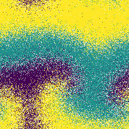
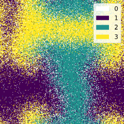
Figure 1: Example model snapshots from the $(3,1)$ May-Leonard system demonstrating different patterns

The $(3,1)$ May-Leonard system, also called the rock-paper-scissors system, is one of the most extensively studied of these stochastic spatial models [2][3][4]. Each vertex in the $(3,1)$ May- Leonard system can have one of four possible states, where state 0 represents an empty vertex, while states 1, 2, and 3 represent different species. The system evolves through diffusion, reproduction, and predation reactions, where species 1 predates on species 2 which predates on species 3 which predates on species 1. This non-transitive competition is one possible explanation for the paradox of the plankton [5] - the mystery of why there are so many more species in the world than simple mathematical models suggest there should be - and has been observed in many real-world ecosystems, including E. Coli bacteria [6], Californian lizards [7], and coral reef invertebrates [8]. On a fully-connected graph, two of the three species in the $(3,1)$ May-Leonard system quickly die out. However, on a lattice, spiral-shaped domains of a single species form, as shown in FIG. 1. Each pixel in FIG. 1 is a vertex on a periodic lattice after the system has run long enough for the pattern to stabilize, with the color denoting the species occupying that vertex. Species 1 chases species 2 across the lattice, species 2 chases species 3, and species 3 chases species 1, with rotating spirals forming where the three domains meet. These domains can form a variety of distinct patterns on the graph, with each picture in FIG. 1 showing an example of a different pattern.

The mobility of a $(3,1)$ May-Leonard system is defined in [2] to be the diffusion rate normalized by the system size. The system has a critical mobility threshold: if the mobility is below the threshold, the model enters a super-persistent transient state and coexistence may be preserved for arbitrarily long time. As the mobility increases, the domains grow wider. Above the critical threshold, the domains outgrow the lattice and two species die out.

However, [2] only studied the critical mobility threshold on the periodic square lattice. Other work has examined random graphs, and lattices with different local neighborhoods [9] [10] [11] [12]. Aside from random graphs, we are unaware of past work that has examined the role of the global graph structure on the critical mobility threshold. A non-periodic lattice was examined in [13], and in fact showed a slightly different critical mobility threshold than [2], but they did not connect this difference to the graph structure.

In this work, we examine the effect of global graph topology on the critical mobility threshold, and show that different graphs have different thresholds. Each graph we study is locally equivalent, but globally distinct. In addition, we use topological data analysis to track the patterns that form on each graph, and show that these differences in critical mobility threshold are caused by topological constraints on which patterns can form on which graph.

Finally, with a few exceptions, e.g. [14], previous researchers of stochastic spatial models have generally not made the code they used publicly available. We describe a new software tool for stochastic spatial models, named Viridicle, which we used to perform the experiments in this paper, and which we release to the community as open source . We additionally make our experimental scripts and experimental data files public.

In Methodology, we describe Viridicle and the analytic methods we use. In Experiments, we use these techniques to explore pattern formation and survival in the $(3,1)$ May-Leonard system on the periodic lattice, on the discretization of the topological 2-sphere, and on the discretization of the Klein bottle. We show experimentally that certain patterns can form only on certain graphs, that each pattern has a distinct median survival duration, and that these result in different critical mobility thresholds. In Discussion, we follow up these experiments by providing a proof that a particular long-lived pattern, which we call the marching bands, cannot form on the sphere, and that this explains its lower critical mobility threshold. In Conclusion, we conclude by summing up our results and discussing directions for future research.

II Methodology

II.1 May-Leonard Models

A stochastic spatial model is a graph where, at time $t$, each vertex $v$ has an associated state $s(v,t)$ taken from a finite set $\mathcal{S}=\{0,1,2,...,n\}$, and the vertex states evolve over time through pair reactions. (Since the units of time are arbitrary in this model, we treat time as unitless.) We assume without loss of generality that our graph is directed, replacing the edges in a non-directed graph with pairs of directed edges, one in each direction. Given a directed edge $e=(v_{1},v_{2})$, where $s(v_{1},t)=s_{1}$ and $s(v_{2},t)=s_{2}$, the time until vertices $v_{1},v_{2}$ change state to $s^{\prime}_{1},s^{\prime}_{2}$, conditioned on no other event occuring first, is exponentially distributed with rate $\rho(s_{1},s_{2},s^{\prime}_{1},s^{\prime}_{2})$, where $\rho$ is a rate tensor . $\rho$ is typically very sparse, and the possible reactions are often described using notation from chemical reactions:

$$(s_{1},s_{2})\to(s_{1}^{\prime},s_{2}^{\prime})\mbox{ at rate }\rho(s_{1},s_{2},s^{\prime}_{1},s^{\prime}_{2})$$

Stochastic spatial models are implemented using the Gillespie algorithm [19]. Given a finite collection of possible events $E_{i}$, where the time to each event is exponentially distributed with rate $\rho_{i}$, the time until some event occurs is exponentially distributed with rate $\rho_{1}+\rho_{2}+...$, and the probability that the next event is $E_{i}$ is $\rho_{i}/(\rho_{1}+...)$. We implement this in a stochastic spatial model by first randomly sampling an edge, then randomly sampling a reaction on that edge. If the randomly selected edge’s vertices $v_{1},v_{2}$ are currently in states $s_{1},s_{2}$, then the probability they transition to states $s_{1}^{\prime},s_{2}^{\prime}$ is:

$$\mathbb{P}((s_{1},s_{2})\to(s_{1}^{\prime},s_{2}^{\prime}))=\frac{\rho(s_{1},s_{2},s_{1}^{\prime},s_{2}^{\prime})}{\rho_{\mbox{max}}}$$

$$\rho_{\mbox{max}}=\max_{s_{1},s_{2}}\left(\sum_{s_{1}^{\prime},s_{2}^{\prime}}\rho(s_{1},s_{2},s_{1}^{\prime},s_{2}^{\prime})\right)$$

Each Gillespie algorithm step accounts for $\rho_{\mbox{max}}N^{-1}$ time, where $N$ is the number of vertices in the graph.

We follow [4] in defining a $(3,1)$ May-Leonard model as a stochastic spatial model with 4 states. State $0$ denotes an empty vertex, while $1,2,3$ all denote vertices occupied by a single individual of that species. The model evolves by three reactions, reproduction, diffusion, and predation:

$$(s,0)\to(s,s)\mbox{ at rate }0.2\mbox{ for }s>0$$

$$(s_{1},s_{2})\to(s_{2},s_{1})\mbox{ at rate }\mu$$

$$(s_{1},s_{2})\to(s_{1},0)\mbox{ at rate }0.2\mbox{ if }s_{1}+1\equiv s_{2}(\mbox{mod }3)\mbox{ and }s_{1},s_{2}>0$$

Where the diffusion rate $\mu$ is a hyperparameter. Following [21], we define the mobility to be $m=\mu(2N)^{-1}$, where $N$ is the number of vertices. The mobility is derived from a scaling term in the asymptotic equivalence of the stochastic spatial model to a PDE, under the assumption our graph consists locally of 2-dimensional von Neumann neighborhoods. Due to differences in how we define the rates and time, our mobilities are not directly comparable to the mobilities in [21], but our results are equivalent up to rescaling.

II.2 Viridicle

To perform our experiments, we have written and make publicly available a software library for simulation of stochastic spatial models, Viridicle. Viridicle is a Python libary written in C, using the NumPy library [22] to allow the user to conveniently pass data to and from the underlying C layer.

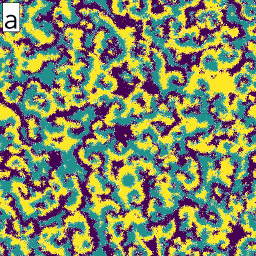
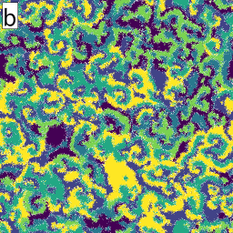
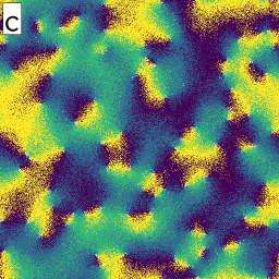
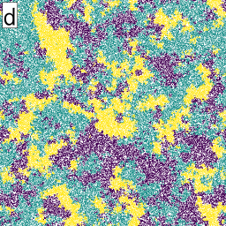
Figure 2: Samples from Viridicle runs of a: $(3,1)$ May-Leonard model [4], b: $(6,3)$ May-Leonard model [4], c: $Z_{N}$ Lotka-Volterra competition [25], and d: Durret & Levin E. Coli model [24]

Viridicle provides a fast implementation of arbitrary stochastic spatial models. It uses a lookup table of pointers to sites to represent the graph edges. This allows the code to support arbitrary, non-lattice graphs without changes to the core functionality. The user can specify a graph structure using the NetworkX libary [23]. We include in the software example implementations of the $(N,r)$ May-Leonard model [2] [4], the Durrett & Levin model of E. Coli bacteria [24], and the Avelino et al model of $Z_{N}$ Lotka-Volterra competition [25]. We show example results for each in FIG. 2; each picture shows a sample graph from one of these models after the model has run long enough for patterns to stabilize. Each pixel represents a vertex in the graph, and different colors represent different model states.

II.3 Pattern Identification

As shown in FIG. 1, the May-Leonard system can form multiple distinct patterns on the lattice. To track the evolution of the pattern over the course of the experiment, we treat the graph as a planar graph and calculate the Betti numbers of the planar subgraphs consisting of all vertices of a specific state. The Betti numbers are invariants of a topological space, equal to the rank of the simplicial homology groups; see [26] for an introduction.

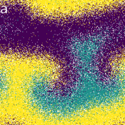
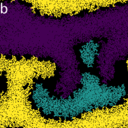
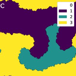
Figure 3: a: Model prior to cleaning; b: Clusters below 128 size are set to 255; c: Clusters are expanded to fill remaining gaps

We first clean the graphs to eliminate small imperfections, such as solitary empty vertices carried into the interior of a domain by diffusion. We define a cluster to be a maximal connected subgraph whose vertices are all the same state. We identify all clusters falling below $N/256$ vertices, where $N$ is the number of vertices in the graph. We set the vertices of those clusters to a null state, distinct from the states 0 through 3 in the model. We then take every vertex in the null state that is adjacent to a vertex of another state, and which is adjacent only to vertices of that state or of null state, and set that vertex to the neighboring vertex’s state. We repeat this process $\sqrt{N}/8$ times. An example of this procedure is shown in FIG. 3.

We then calculate the 0th and 1st Betti numbers of the subgraphs of all vertices belonging to each state. In a closed 2-dimensional manifold, $b_{0}$ is equal to the number of clusters, and $b_{1}$ can be calculated by Euler’s formula:

$$b_{1}=b_{0}-\chi+b_{2}$$

$$\chi=(\#\mbox{ of vertices})+(\#\mbox{ of edges})-(\#\mbox{ of faces})$$

The second Betti number, $b_{2}$, is 1 if the subgraph contains the entire graph and the graph is the discretization of an orientable manifold; otherwise it is 0. We define $b_{i}(s)$ to be the $i$th Betti number of the subgraph of all vertices, edges, and faces of state $s$.

During each experiment, we calculated the Betti numbers of each state every 1.0 time. We sort the Betti numbers for states 1, 2, and 3 and concatenate them so that the resulting pattern codes are invariant under permutation of the non-empty states. For example, FIG. 3 is in state 111011: the 0th Betti number of all three states are 1, the 1st Betti number of states 1 and 3 are 1, and the 1st Betti number of state 2 is 0.

Finally, in order to eliminate transitory fluctuations that represent flaws in our analytic procedure rather than genuine changes in the system, we reclassified any pattern that lasted for less than 5.0 time as “transitory”. If the system entered a transitory state for 5.0 or less time and then returned to its original state, we removed that transitory fluctuation, reclassifying it as the surrounding pattern.

III Experiments

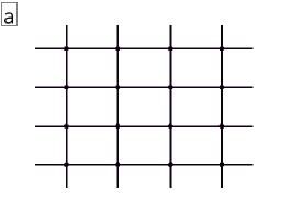
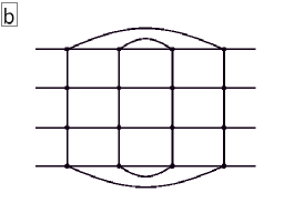
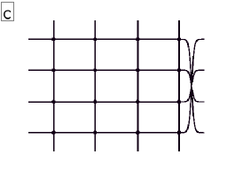
Figure 4: a: $4\times 4$ periodic lattice, b: sphere, and c: Klein bottle. The edges of each image are periodic.

We explored the effect of graph topology on the critical mobility threshold of the $(3,1)$ May-Leonard system using three graphs, as shown in FIG. 4: a 2-dimensional periodic lattice, equivalent to a discretization of a torus; a 2-dimensional lattice with edges wrapped to form a discretization of a topological 2-sphere; and a 2-dimensional lattice with the edges wrapped to form a Klein bottle. These graphs are all locally equivalent, but have distinct global topologies.

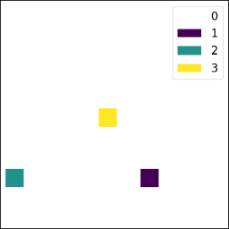
Figure 5: Example of block initialization - blocks are placed randomly on the lattice.

We began by exploring feasible patterns that could occur on each graph. We experimented with random initializations, as used in [2] and [13], but we found that we could achieve coexistence at higher mobility using a structured initialization. We initialized the lattice in state 0, then placed one block of each state in random non-overlapping locations on it, as shown in FIG. 5. We used four choices of lattice width, 32, 64, 128, and 256 vertices, and sampled a variety of mobilities between $1\times 10^{-4}$ and $8\times 10^{-4}$. We ran 256 experiments on AWS EC2 for each combination of hyperparameters, running each experiment for 1000.0 time.

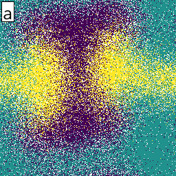
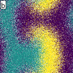
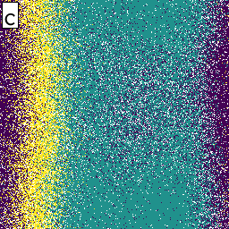
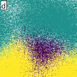
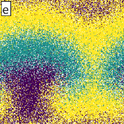
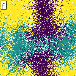
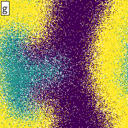
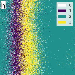
Figure 6: Top row: lattice. a: Pattern code 111001, b: 111011, c: 111111. Middle row: sphere. d: 111000, e: 121001. Bottom row: torus. f: 111001, g: 111011, h: 111111. 111111 are the “marching bands.”

We calculated the pattern codes of each experiment every 1.0 time, giving us the 0th and 1st Betti numbers of the planar subgraphs consisting of all vertices of a particular state, sorted so as to be invariant to permutations of the non- empty state. We ignored patterns before 200 time, as these might be transients during system warmup. We also ignored patterns with a zero 0th Betti number for a non-empty state, as these are patterns where no species has gone extinct yet, but where some species has become so rarefied that it is eliminated by the cleaning process. Recovery from this state is rare, and does not significantly contribute to survival time. We looked for patterns for which we had at least one example that persisted for more than 100.0 time when $m\geq 2.5\times 10^{-4}$. This gave us three patterns on the Klein bottle, two on the sphere, and three on the torus. Examples of each pattern are shown in FIG. 6.

We saved the model state at the start of periods where the system remains in the same pattern for at least 100.0 time. We randomly sampled from these saved states as initializations and ran 256 additional experiments with new random seeds for each combination of graph, pattern, and width greater than 32, and a selection of mobilities. We excluded width 32 as the models were so unstable we could not gather enough initializations. For mobilities with insufficient examples, we sampled additional saved states from neighboring mobilities to ensure we had at least 64 initializations. We refer to these as patterned initializations, since they are intended to induce the formation of a specific pattern at the start of the experiment. We ran the models to see how long each pattern would last before transitioning to a new pattern, discarding experiments where, despite the initialization, the desired pattern did not form.

IV Results and Discussion

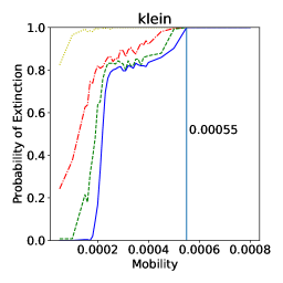
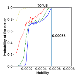
Figure 7: Probability of extinction by 1000 time versus mobility, from experiments with block initialization. Each curve represents a different lattice size. Vertical lines are drawn at the mobility threshold where $99\%$ of all experiments see at least one species go extinct by 1000 time.

In FIG. 7, we show the extinction curves of our experiments with block initialization. Each curve gives the probability that, in a system beginning with block initialization, at least one species will have gone extinct by the end of the experiment at 1000.0 time. We observe that the critical mobility threshold of the sphere is about $2.8\times 10^{-4}$ while the critical mobility threshold of the torus and the Klein bottle are both about $5.5\times 10^{-4}$, implying that the large-scale graph structure does have a significant effect on the critical mobility threshold.

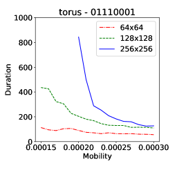
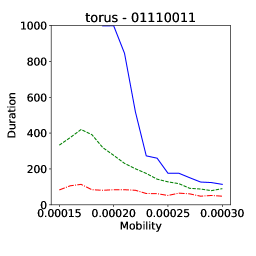
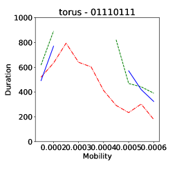
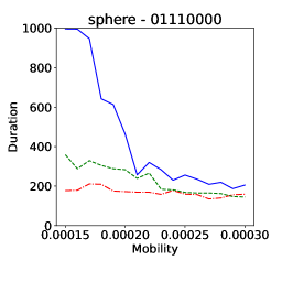
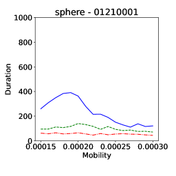
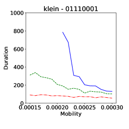
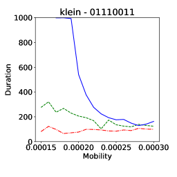
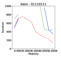
Figure 8: Median survival times vs mobility for each pattern from experiments with patterned initializations. Note range of horizontal axis is not consistent. Titles show graph type and pattern code. We omit portions of the curve where the median pattern cannot be estimated because fewer than 50% of the experiments had collapsed by 1000 time.

In FIG. 8, we show the median duration of each long- lived pattern from our experiments with patterned initializon, estimated using the Kaplan-Meier estimator [27] [28]. We observe that each pattern has a distinct median survival time, and that the survival of the torus and Klein bottle graphs at higher mobilities is due to a specific pattern, 111111. We dub this pattern the marching bands, since it consists of three bands of different states “marching” across the lattice, state 1 chasing state 2 chasing state 3 chasing state 1. The marching bands pattern is extremely stable, likely due to the absence of spirals, since there is no point on the marching bands where all three states meet.

It is easy to show that topological constraints make it impossible for the marching bands to form on the sphere. In what follows, $H_{k}(X)$ is the $k$th simplicial homology group of the manifold $X$.

Theorem 1.

Let $U_{1},U_{2},U_{3}\subset S^{2}$ be connected, non- empty, open sets such that $\overline{U_{1}}\cup\overline{U_{2}}\cup\overline{U_{3}}=S^{2}$ and $U_{i}\cap U_{j}$ is empty for $i\neq j$. There exists no choice of $U_{i}$ such that $H_{1}(U_{1})\cong H_{1}(U_{2})\cong\mathbb{Z}$.

Proof.

Since $U_{i}$ are connected surfaces that are subsets of $S^{2}$, they must be orientable, possibly punctured, genus-0 surfaces. Therefore, they are classified by their first homology group, so $U_{1}$ must be a neighborhood of a circle, and $\partial U_{1}$ must be a disjoint pair of circles.

Let $\widetilde{U}_{i}$ be arbitrarily small neighborhoods of $U_{i}$, and let $V=\widetilde{U}_{2}\cup\widetilde{U}_{3}$. Then $V\cap\widetilde{U}_{1}$ is an arbitrarily small neighborhood of $\partial U_{1}$, and must have homology groups $H_{0}(V\cap\widetilde{U}_{1})\cong H_{1}(V\cap\widetilde{U}_{1})\cong\mathbb{Z}^{2},H_{2}(V\cap\widetilde{U}_{1})\cong\varnothing$.

By the Mayer-Veitoris Theorem, there is a pair of long exact sequences:

$$\varnothing\to H_{2}(S^{2})\to H_{1}(V\cap\widetilde{U}_{1})\to$$

$$H_{1}(V)\oplus H_{1}(\widetilde{U}_{1})\to H_{1}(S^{2})\to...$$

$$...\to H_{1}(S^{2})\to H_{0}(V\cap\widetilde{U}_{1})\to$$

$$H_{0}(V)\oplus H_{0}(\widetilde{U}_{1})\to H_{0}(S^{2})\to\varnothing$$

Which is equivalent to:

$$\varnothing\to\mathbb{Z}\to\mathbb{Z}^{2}\to H_{1}(V)\oplus\mathbb{Z}\to\varnothing$$

$$\varnothing\to\mathbb{Z}^{2}\to H_{0}(V)\oplus\mathbb{Z}\to\mathbb{Z}\to\varnothing$$

From which we conclude that $H_{1}(V)\cong\varnothing,H_{0}(V)\cong\mathbb{Z}^{2}$. Therefore, $V$ has two components, both of which are orientable open surfaces with genus zero and no punctures. Since $\widetilde{U}_{2},\widetilde{U}_{3}$ are both connected, each must correspond to one of those two components, and so $H_{1}(U_{2})\cong H_{1}(U_{3})\cong\varnothing$.

∎

Corollary 2.

The marching bands cannot form on a spherical graph.

Proof.

This is immediate from Theorem 1.∎

However, the existence of the marching bands is not the sole distinction between the graphs. We find that if we eliminate the marching bands, the spherical graph actually has a slightly higher critical mobility. In FIG. 9, we plot the probability that at least one species goes extinct by 1000.0 time for our experiments using block initialization, excluding experiments that entered the marching bands pattern at any time. We observe that, excluding experiments that entered the marching bands, the critical mobility threshold of the periodic lattice and the Klein bottle are both $2.5\times 10^{-4}$, compared to $2.8\times 10^{-4}$. This implies that the effect of graph topology is not limited to the ability of the torus and Klein bottle to support patterns without spirals, because even in spiraling patterns, the critical mobility threshold of the sphere is slightly different.

Interestingly, the non-orientability of the Klein bottle appears to have no impact on the critical mobility threshold. The Klein bottle has higher probability of extinction for a given mobility, but the critical mobility thresholds are identical. We attribute this to the fact that the marching bands can only form in one direction on the Klein bottle, as opposed to two on the torus, making it less likely this pattern will form during model warmup.

V Conclusions and Further Research

In this work we have shown that the critical mobility threshold of the $(3,1)$ May-Leonard system is a property of the global graph structure, due to topological constraints on which patterns can form on which graphs.

Future research will focus on a more detailed understanding of the role topology plays in what patterns can form and how they evolve. The Betti number calculation we used is tractable only for discretizations of 2-dimensional manifolds; finding a more general homological calculation would allow us to extend this analysis to other graphs.

VI Figures

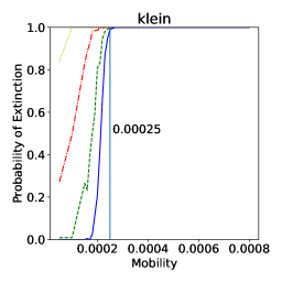
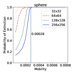
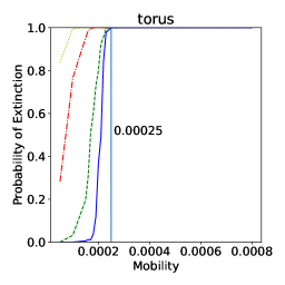
Figure 9: Probability of extinction by 1000 time versus mobility, from experiments with block initialization, excluding experiments that entered the marching bands pattern. Each curve represents a different lattice size. Vertical lines are drawn at the mobility threshold where $99\%$ of all experiments see at least one species go extinct by 1000 time.

References

- Durret and Levin [1994] R. Durret and S. Levin, Stochastic spatial models: A user’s guide to ecological applications, Philosophical Transactions of the Royal Society B 343 (1994).
- Reichenbach et al. [2007] T. Reichenbach, M. Mobilia, and E. Frey, Mobility promotes and jeopardizes biodiversity in rock-paper-scissors games, Nature 448, 1046 (2007).
- May and Leonard [1977] R. M. May and W. J. Leonard, Nonlinear aspects of competition between three species, SIAM Journal on Applied Mathematics 29, 243 (1977).
- Roman et al. [2013] A. Roman, D. Dasgupta, and M. Pleimling, Interplay between formation and competition in generalized may-leonard games, Physical Review E 87 (2013).
- Hutchinson [1960] G. E. Hutchinson, The paradox of the plankton, American Naturalist 95, 137 (1960).
- Kirkup and Riley [2004] B. C. Kirkup and M. A. Riley, Antibiotic-mediated antagonism leads to a bacterial game of rock-paper-scissors in Vivo, Nature 428, 412 (2004).
- Sinervo and Lively [1996] B. Sinervo and C. Lively, The rock-paper-scissors game and the evolution of alternative male strategies, Nature 380, 240 (1996).
- Jackson and Buss [1975] J. B. C. Jackson and L. Buss, Alleopathy and spatial competition among coral reef invertebrates, Proceedings of the National Academy of Sciences 72, 5160 (1975).
- Perc et al. [2007] M. Perc, A. Szolnoki, and G. Szabó, Cyclical interactions with alliance-specific heterogenous invasion rates, Physical Review E 75 (2007).
- Szczesny et al. [2013] B. Szczesny, M. Mobilia, and A. Rucklidge, When does cyclic dominance lead to stable spiral waves?, EuroPhysics Letters 102 (2013).
- Szolnoki and Szabo [2004] A. Szolnoki and G. Szabo, Phase transitions for rock-scissors-paper game on different networks, Physical Review E 70 (2004).
- Calleja-Solanas et al. [2020] V. Calleja-Solanas, N. Khalil, E. Hernandez-Garcia, J. Gomez-Gardenes, and S. Meloni, Structured interactions as a stabilizing mechanism for competitive ecosystems, (2020), arXiv:2012.14916 [q-bio.PE] .
- Chen et al. [2014] H. Chen, N. Yao, Z.-G. Huang, J. Park, Y. Do, and Y.-C. Lai, Mesoscopic interactions and species coexistence in evolutionary game dynamics of cyclic competitions, Scientific Reports 4 (2014).
- Pires et al. [2021] M. A. Pires, N. Crokidakis, and S. M. Duarte Queirós, Diffusion plays an unusual role in ecological quasi-neutral competition in metapopulations, Nonlinear Dynamics 103, 1219 (2021).
- Note [1] https://github.com/TheoremEngine/Viridicle.
- Note [2] https://github.com/TheoremEngine/graph-topology-determines-survival.
- Note [3] https://www.theorem-engine.com/papers/001/index.html.
- Note [4] There is some disagreement in the literature on the best approach to defining rates. It is common to define the rate as the rate at which a transition occurs on a vertex, e.g., [2]. We choose to define the rate as the rate at which an event occurs on a directed edge because this allows significant computational savings: we can sample the next vertex pair by sampling from a list of directed edges, which requires a single RNG call, rather than by first sampling a vertex and then sampling a neighbor of that vertex, which requires two. The two approachs are equivalent up to a rescaling of time on a regular graph, and all graphs we explore are regular.
- Gillespie [1977] D. Gillespie, Exact stochastic simulation of coupled chemical reactions, The Journal of Physical Chemistry 81, 2340 (1977).
- Note [5] Some past work, e.g. [2], instead defines one step as taking time; the two approaches are equivalent up to rescaling of time.
- Reichenbach et al. [2008] T. Reichenbach, M. Mobilia, and E. Frey, Self-organization of mobile populations in cyclic competition, Journal of Theoretical Biology 254, 368 (2008).
- Harris et al. [2020] C. R. Harris, K. J. Millman, S. J. van der Walt, R. Gommers, P. Virtanen, D. Cournapeau, E. Wieser, J. Taylor, S. Berg, N. J. Smith, R. Kern, M. Picus, S. Hoyer, M. H. van Kerkwijk, M. Brett, A. Haldane, J. F. del Río, M. Wiebe, P. Peterson, P. Gérard-Marchant, K. Sheppard, T. Reddy, W. Weckesser, H. Abbasi, C. Gohlke, and T. E. Oliphant, Array programming with NumPy, Nature 585, 357 (2020).
- Hagberg et al. [2008] A. Hagberg, D. Schult, and P. Swart, Exploring network structure, dynamics, and function using NetworkX, Proceedings of the 7th Python in Science Conference (SciPy2008), (2008).
- Durret and Levin [1997] R. Durret and S. Levin, Allelopathy in spatially distributed populations, Journal of Theoretical Biology 185, 165 (1997).
- Avelino et al. [2014] P. P. Avelino, D. Bazeia, J. Menezes, and B. F. de Oliveira, String networks in lotka-volterra competition models, Physics Letters A 378, 393 (2014).
- Hatcher [2001] A. Hatcher, Algebraic Topology (Cambridge University Press, 2001).
- Kaplan and Meier [1958] E. L. Kaplan and P. Meier, Nonparametric estimation from incomplete observations, Journal of the American Statistical Association 53, 457 (1958).
- Davidson-Pilon et al. [2021] C. Davidson-Pilon, J. Kalderstam, N. Jacobson, S. Reed, B. Kuhn, P. Zivich, M. Williamson, AbdealiJK, D. Datta, A. Fiore-Gartland, A. Parij, D. Wilson, Gabriel, L. Moneda, A. Moncada-Torres, K. Stark, H. Gadgil, Jona, K. Singaravelan, L. Besson, M. S. Peña, S. Anton, A. Klintberg, GrowthJeff, J. Noorbakhsh, M. Begun, R. Kumar, S. Hussey, S. Seabold, and D. Golland, Camdavidsonpilon/lifelines: v0.25.9 (2021).