Sharp Bounds for Federated Averaging (Local SGD)
and Continuous Perspective

Abstract

Federated Averaging (FedAvg), also known as Local SGD, is one of the most popular algorithms in Federated Learning (FL). Despite its simplicity and popularity, the convergence rate of FedAvg has thus far been undetermined. Even under the simplest assumptions (convex, smooth, homogeneous, and bounded covariance), the best known upper and lower bounds do not match, and it is not clear whether the existing analysis captures the capacity of the algorithm. In this work, we first resolve this question by providing a lower bound for FedAvg that matches the existing upper bound, which shows the existing FedAvg upper bound analysis is not improvable. Additionally, we establish a lower bound in a heterogeneous setting that nearly matches the existing upper bound. While our lower bounds show the limitations of FedAvg, under an additional assumption of third-order smoothness, we prove more optimistic state-of-the-art convergence results in both convex and non-convex settings. Our analysis stems from a notion we call iterate bias, which is defined by the deviation of the expectation of the SGD trajectory from the noiseless gradient descent trajectory with the same initialization. We prove novel sharp bounds on this quantity, and show intuitively how to analyze this quantity from a Stochastic Differential Equation (SDE) perspective.

1 Introduction

Federated Learning (FL) is an emerging distributed learning paradigm in which a massive number of clients collaboratively participate in the training process without disclosing their private local data to the public (Konecny et al., 2015). Typically, federated learning is orchestrated by a central server who oversees the clients, e.g. mobile devices or a group of organizations. The training process combines local training of a model at the clients with infrequent aggregation of the locally trained models at the central server.

Reflecting the goal of minimizing a loss function aggregated across clients, we consider the distributed optimization problem $\min F(\mathbf{x}):=\frac{1}{M}\sum_{m=1}^{M}F_{m}(\mathbf{x}),$ where each client $m\in[M]$ holds a local objective $F_{m}$ realized by its local data distribution $\operatorname{\mathcal{D}}_{m}$, namely $F_{m}(\mathbf{x}):=\mathbb{E}_{\xi\sim\mathcal{D}_{m}}f(\mathbf{x};\xi).$ Federated Learning is heterogeneous by design as $\mathcal{D}_{m}$ can vary across clients. In the special case when $\mathcal{D}_{m}\equiv\mathcal{D}$ for all clients $m$, the problem is called homogeneous.

Federated Averaging (FedAvg, McMahan et al. 2017), also known as Local SGD (Stich 2019), is one of the most popular algorithms applied in Federated Learning. In its simplest form, FedAvg proceeds in $R$ communication rounds, where at the beginning of each round, a central server sends the current iterate to each of the $M$ clients. Each client then locally takes $K$ steps of SGD, and then returns its final iterate to the central server. The central server averages these iterates to obtain the first iterate of the next round. We state the FedAvg algorithm formally in Algorithm 1.

Table 1: Convergence Rates of FedAvg. Some lower order terms as $R\rightarrow\infty$ omitted. $H$: smoothness, $R$: number of rounds, $K$: local iterations per round, $M$: number of clients, $\sigma$: noise, $D:\|\mathbf{x}^{(0,0)}-\mathbf{x}^{\star}\|.$ The lower and upper bound use a slightly different metric of heterogeneity ($\zeta$ and $\zeta_{*}$), see Remark 3.2 for details. We bold the terms where our analysis improves upon previous work.

	Homogeneous (Assumption 1)	Heterogeneous (Assumption 1 and 3)
Previous Upper Bound	$\frac{HD^{2}}{KR}+\frac{\sigma D}{\sqrt{MKR}}+\frac{H^{\frac{1}{3}}\sigma^{\frac{2}{3}}D^{\frac{4}{3}}}{K^{\frac{1}{3}}R^{\frac{2}{3}}}$	$\frac{HD^{2}}{KR}+\frac{\sigma D}{\sqrt{MKR}}+\frac{H^{\frac{1}{3}}\sigma^{\frac{2}{3}}D^{\frac{4}{3}}}{K^{\frac{1}{3}}R^{\frac{2}{3}}}+\frac{H^{\frac{1}{3}}\zeta^{\frac{2}{3}}D^{\frac{4}{3}}}{R^{\frac{2}{3}}}$
	(Khaled et al., 2020)	(Khaled et al., 2020; Woodworth et al., 2020a)
Our Lower Bound	${\bf{\frac{HD^{2}}{KR}}}+\frac{\sigma D}{\sqrt{MKR}}+\frac{H^{\frac{1}{3}}\sigma^{\frac{2}{3}}D^{\frac{4}{3}}}{{\bf{K^{\frac{1}{3}}}}R^{\frac{2}{3}}}$	$\frac{HD^{2}}{KR}+\frac{\sigma D}{\sqrt{MKR}}+\frac{H^{\frac{1}{3}}\sigma^{\frac{2}{3}}D^{\frac{4}{3}}}{{\bf{K^{\frac{1}{3}}}}R^{\frac{2}{3}}}+{\bf{\frac{H^{\frac{1}{3}}\zeta^{\frac{2}{3}}_{*}D^{\frac{4}{3}}}{R^{\frac{2}{3}}}}}$
	Theorem 3.1	Theorem 3.3
Previous Lower Bound	$\frac{\sigma D}{\sqrt{MKR}}+\frac{H^{\frac{1}{3}}\sigma^{\frac{2}{3}}D^{\frac{4}{3}}}{{\bf{K^{\frac{2}{3}}}}R^{\frac{2}{3}}}$	$\frac{\sigma D}{\sqrt{MKR}}+\frac{H^{\frac{1}{3}}\sigma^{\frac{2}{3}}D^{\frac{4}{3}}}{{\bf{K^{\frac{2}{3}}}}R^{\frac{2}{3}}}+{\bf{\min\left(\frac{HD^{2}}{R},\frac{H^{\frac{1}{3}}\zeta^{\frac{2}{3}}_{*}D^{\frac{4}{3}}}{R^{\frac{2}{3}}}\right)}}$
	(Woodworth et al., 2020b)	(Woodworth et al., 2020a)

While the FedAvg algorithm is popular in practice, a thorough theoretical understanding of FedAvg has not been established. Even under the simplest setting (convex, smooth, homogeneous and bounded covariance, see Assumption 1), the state-of-the-art upper bounds for FedAvg due to Khaled et al. (2020) and Woodworth et al. (2020b) do not match the state-of-the-art lower bound due to Woodworth et al. (2020b), see Table 1. This suggests that at least one side of the analysis is not sharp. Therefore a fundamental question remains:

Does the current convergence analysis of FedAvg fully capture the capacity of the algorithm?

Our first contribution is to answer this question definitively under the standard smoothness and convexity assumptions. We establish a sharp lower bound for FedAvg that matches the existing upper bound (Theorem 3.1), showing that the existing FedAvg analysis is not improvable. Moreover, we establish a stronger lower bound in the heterogeneous setting, Theorem 3.3, which suggests the best known heterogeneous upper bound analysis (Woodworth et al., 2020a) is also (almost) not improvable.

Algorithm 1 Federated Averaging (FedAvg)

1:  procedure FedAvg ($\mathbf{x}^{(0,0)},\eta$)

2:  for $r=0,\ldots,R-1$ do

3:    on client for $m\in[M]$ in parallel do

4:      $\mathbf{x}_{m}^{(r,0)}\leftarrow\mathbf{x}^{(r,0)}$ $\vartriangleright$ broadcast current iterate

5:      for $k=0,\ldots,K-1$ do

6:         $\xi^{(r,k)}_{m}\sim\mathcal{D}_{m}$

7:         $\mathbf{g}^{(r,k)}_{m}\leftarrow\nabla f(\mathbf{x}^{(r,k)}_{m};\xi^{(r,k)}_{m})$

8:         $\mathbf{x}^{(r,k+1)}_{m}\leftarrow\mathbf{x}^{(r,k)}_{m}-\eta\cdot\mathbf{g}_{m}^{(r,k)}$ $\vartriangleright$ client update $\mathbf{x}^{(r+1,0)}\leftarrow\frac{1}{M}\sum_{m=1}^{M}\mathbf{x}^{(r,K)}_{m}$ $\vartriangleright$ server averaging

Our proofs highlight exactly what can go wrong in FedAvg, yielding these slow convergence rates. Specifically, our lower bound analysis stems from a notion we call iterate bias, which is defined by the deviation of the expectation of the SGD trajectory from the (noiseless) gradient descent trajectory with the same initialization (see Definition 2.1 for details). We show that even for convex and smooth objectives, the mean of SGD initialized at the optimum can drift away from the optimum at the rate of $\Theta(\eta^{2}k^{\frac{3}{2}})$ after $k$ steps, for sufficiently small learning rate $\eta$. We depict this phenomenon in Fig. 1.The iterate bias thus quantifies the fundamental difficulty encountered by FedAvg:

Even with infinite number of homogeneous clients, FedAvg can drift away from the optimum even if initialized at the optimum.

Indeed, we show in Section 3.2 that the sharp lower bound of SGD iterate bias leads directly to our sharp lower bound of FedAvg convergence rate.

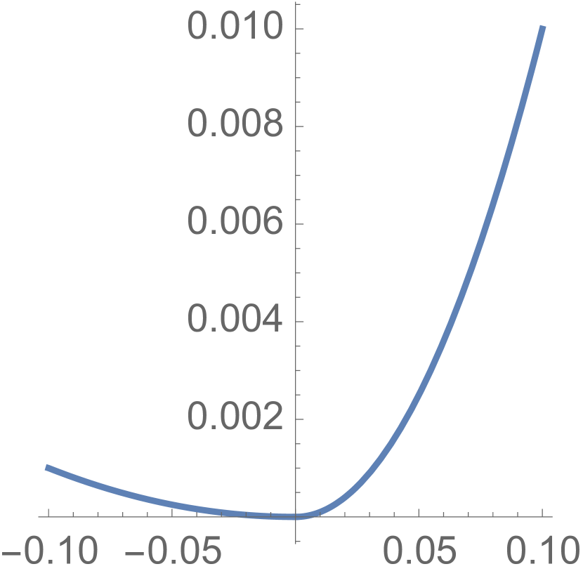
(a) Function plot

(b) Probability density function after various SGD steps

Figure 1: Illustration of the iterate bias of SGD. Consider the objective $F(x)=\begin{cases}x^{2}&x\geq 0\\ \frac{1}{10}x^{2}&x<0\end{cases}$ as shown in (a), and $f(x;\xi):=\xi x+F(x)$ where $\xi\sim\mathcal{N}(0,0.01)$. We initialize the SGD at optimum $x^{\star}=0$, and run 1024 steps of SGD with step size $10^{-2}$. We repeat this random process for 65536 times, and estimate the density function after 128, 256, 512 and 1024 steps. Observe that the density function and the average gradually move to the left (away from the optimum, where the curvature is smaller). This figure explains the intrinsic difficulty for FedAvg to handle objective with drastic Hessian change.

The discouraging lower bound of FedAvg under a standard smoothness assumption does not conform well with its empirical efficiency observed in practice (Lin et al., 2020c). This motivates us to consider whether additional modeling assumptions could better explain the empirical performance of FedAvg. The aforementioned lower bound is attained by a special piece-wise quadratic function with a sudden curvature change, which is smooth (has bounded second-order derivatives) but has unbounded third-order derivatives. A natural assumption to exclude this corner case is third-order smoothness, which has been considered before in the context of federated learning (Yuan and Ma, 2020), and may be representative of objectives in practice. For instance, loss functions used to learn many generalized linear models, such as logistic regression, often exhibit third-order smoothness (Hastie et al., 2009).

With this third-order smoothness assumption, we show that the iterate bias reduces to $\Theta(\eta^{3}k^{2})$, one order higher in $\eta$ than the rate under only second-order smoothness. While the proofs for bounding the iterate bias are quite technical, we show that it is easy to analyze the bias via a continuous approach. More specifically, by studying the stochastic differential equation (SDE) corresponding to the continuous limit of SGD, one can derive the limit of the iterate bias of generic objectives by using the Kolmogorov backward equation of the SDE, see Section 2.3.

Leveraging this intuition from the bias, we prove state-of-the-art rates for FedAvg under third-order smoothness in both convex and non-convex settings (Theorems 4.1 and 4.2). In non-convex settings, our convergence rate scales with $1/R^{\frac{4}{5}}$, which improves upon the best known rate of $1/R^{\frac{2}{3}}$ (Yu et al., 2019b) if we do not assume third-order smoothness.

1.1 Related Work

FedAvg Analysis.

The understanding of local updates algorithm such as FedAvg is one of the most important topics in distributed optimization. The early analysis of FedAvg preceded the proposal of Federated Learning, typically under the name of Local SGD or parallel SGD (Mcdonald et al., 2009; Zinkevich et al., 2010; Shamir and Srebro, 2014; Rosenblatt and Nadler, 2016; Jain et al., 2018; Zhou and Cong, 2018). The primary focus of this literature is the special case of one-shot averaging, in which only one round of averaging (communication) is conducted at the end of the algorithm. The first upper bound of FedAvg (with multiple averaging rounds) was established by Stich (2019) in the convex homogeneous setting, which imposes uniform gradient bound assumption. The result was further improved by Khaled et al. (2020); Woodworth et al. (2020b) with improved rates and relaxed assumptions. Note that the result of Khaled et al. (2020) preceded that of Woodworth et al. (2020b), but the step-size was not properly optimized. In the convex heterogeneous setting, the first upper bound of FedAvg is due to Li et al. (2020c). This result was improved by Khaled et al. (2020); Woodworth et al. (2020a). For non-convex objectives, a series of recent works (Zhou and Cong, 2018; Haddadpour et al., 2019; Wang and Joshi, 2018; Yu and Jin, 2019; Yu et al., 2019a) has established various upper bounds of FedAvg in homogeneous and heterogeneous settings. On the lower bound side, the best known result for convex FedAvg is established by Woodworth et al. (2020b) (for homogeneous) and Woodworth et al. (2020a) (for heterogeneous). To the best of our knowledge, we are unaware of any lower bound for FedAvg in non-convex settings.

The existence and effect of iterate bias has been observed in various forms in the current literature (Dieuleveut et al., 2020; Charles and Konečný, 2020; Woodworth et al., 2020b), yet our paper is the first to sharply characterize the rate of the bias, both in the second-order smooth case and third-order smooth case.

Other Extensions of FedAvg.

Throughout this work, we study the simplest form of FedAvg (Algorithm 1) to keep our efforts focused. There are many other extensions of FedAvg applied in practice. For example, instead of letting all the clients to participate in computation, one may randomly draw a subset of clients to participate every round. Most of our results (e.g., all of the homogeneous results) can be directly extended to this sub-sampling variant. Other variants of FedAvg include letting clients run different number of steps per round, or average the client states non-uniformly. We refer readers to Wang et al. (2021) for a more comprehensive survey of these extensions.

One special extension of FedAvg introduces a “server learning rate”, which we name FedAvg-SLR to distinguish it. Instead of taking the client averaging as the initialization of the next round, FedAvg-SLR extrapolates (or interpolates) between the round initialization and the clients averaging (Charles and Konečný, 2020; Reddi et al., 2021), or formally $\mathbf{x}^{(r+1,0)}\leftarrow\mathbf{x}^{(r,0)}+\eta_{s}\cdot\frac{1}{M}\sum_{m=1}^{M}\left(\mathbf{x}_{m}^{(r,K)}-\mathbf{x}^{(r,0)}\right).$ By definition, FedAvg-SLR reduces to the classic FedAvg when $\eta_{s}=1$. Notably, FedAvg-SLR also reduces to mini-batch SGD when the client learning rate goes to 0, and the server learning rate goes to infinity. Therefore, FedAvg-SLR can at least attain the best convergence rate of the classic FedAvg and the mini-batch SGD. However, to the best of our knowledge, it is not known whether FedAvg-SLR can outperform the best of the two, and there are no results that characterize FedAvg-SLR beyond the two special regimes. While our lower bounds do not apply to the generic form of FedAvg-SLR, we anticipate that our techniques (e.g., iterate bias) can be applicable to the study of FedAvg-SLR in the future work.

Other Federated Learning Algorithms.

Besides the FedAvg framework, there are many other federated optimization algorithms that aims to improve communication efficiency (Yuan and Ma, 2020; Reddi et al., 2021) or tackle the heterogeneity in FL (Li et al., 2020b; Karimireddy et al., 2020). We expect the techniques developed in this work can shed light on the analysis of broader existing federated algorithms and promote the design of more efficient federated algorithms.

The past half decade has witnessed a booming interest in various aspects of Federated Learning. Data heterogeneity is one of the most important patterns in Federated Learning, and is known to cause performance degradation in practice (Hsu et al., 2019). Numerous existing works have aimed to understand and mitigate the negative effect of heterogeneity in various ways (Mohri et al., 2019; Liang et al., 2019; Chen et al., 2020; Deng et al., 2020; Li et al., 2020a; Reisizadeh et al., 2020; Wang et al., 2019; Pathak and Wainwright, 2020; Zhang et al., 2020; Yuan et al., 2021b; Acar et al., 2021a; Al-Shedivat et al., 2021; Yuan et al., 2021a). In practice, the system heterogeneity will also affect the performance of Federated Learning (Smith et al., 2017; Diao et al., 2021). In deep learning context, a recent array of works has studied the alternative approaches of model ensembling beyond averaging in parameter space (Bistritz et al., 2020; He et al., 2020; Lin et al., 2020b; Chen and Chao, 2021; Yoon et al., 2021).

This paper mainly considers the classic FL settings in which the same model is learned from and deployed to all the clients. There is an alternative setup in FL, known as the personalized setting, which aims to learn a different (personalized) model for different clients. Numerous recent papers have proposed Federated Learning models and algorithms to accommodate personalization (Smith et al., 2017; Jiang et al., 2019; Chen et al., 2019; Fallah et al., 2020; Hanzely et al., 2020; London, 2020; T. Dinh et al., 2020; Hanzely and Richtárik, 2020; Agarwal et al., 2020; Lin et al., 2020a; Deng et al., 2020; Acar et al., 2021b). We anticipate the techniques developed in this work can be applied to personalized FL algorithms, especially the ones that applied local updates approach.

We refer readers to (Kairouz et al., 2019; Wang et al., 2021) for a more comprehensive survey on the recent progress of Federated Learning.

Connection to Implicit Bias.

It is possible to view the iterate bias as an implicit bias of the FedAvg algorithm, which pushes the iterate towards flatter regions of the objective. This effect is similar to other instances of implicit bias observed for stochastic gradient descent, which has drawn connections between noise in the gradients and flat minima (Hochreiter and Schmidhuber, 1997; Jastrzkebski et al., 2017; Blanc et al., 2020; Damian et al., 2021). While in many instances, implicit bias has been linked to choosing favorable optima that generalize well (Neyshabur, 2017), in our setting, the bias affects the convergence rate.

1.2 Organization and Notation

In Section 2, we formally define the iterate bias of SGD, and state sharp bounds on its rate. In Section 3, we state our lower bounds for FedAvg, and show how the iterate bias can be used to achieve our sharp bounds. In Section 4, we state our convergence results for FedAvg under third-order smoothness. All proofs are deferred to the appendix.

We use bold lower case character to denote vectors (e.g., $\mathbf{x}$). We use $\|\cdot\|$ to denote the $\ell_{2}$-norm of a vector, $[n]$ to denote the set $\{1,\ldots,n\}$. Throughout the paper, we use $O,\Omega,\Theta$ notation to hide absolute constants only.

2 Setup and Technical Overview: Intuition From Iterate Bias of SGD

The intuition from our lower bound comes from studying the behaviour of FedAvg when the number of clients, $M$, tends to infinity. In this case, the averaged iterate $\mathbf{x}^{(r+1,0)}$ is precisely the expected iterate after $K$ iterations of SGD starting from the last averaged iterate, $\mathbf{x}^{(r,0)}$. This motivates the following definition.

Definition 2.1 (Iterate Bias of SGD).

Let $\{\mathbf{x}_{\mathtt{SGD}}^{(k)}\}_{k=0}^{\infty}$ and $\{\mathbf{z}_{\mathtt{GD}}^{(k)}\}_{k=0}^{\infty}$ be the trajectories of SGD and GD initialized at the same point $\mathbf{x}$, formally

$$\mathbf{x}^{(k+1)}_{\mathtt{SGD}}\leftarrow\mathbf{x}_{\mathtt{SGD}}^{(k)}-\eta\nabla f(\mathbf{x}_{\mathtt{SGD}}^{(k)};\xi^{(k)}),\qquad \mathbf{x}_{\mathtt{SGD}}^{(0)}=\mathbf{x};$$

$$\mathbf{z}^{(k+1)}_{\mathtt{GD}}\leftarrow\mathbf{z}_{\mathtt{GD}}^{(k)}-\eta\nabla F(\mathbf{z}_{\mathtt{GD}}),\qquad \mathbf{z}_{\mathtt{GD}}^{(0)}=\mathbf{x}.$$

The iterate bias (or in short “bias”) from $\mathbf{x}$ at the $k$-th step is defined as

$$\operatorname{\mathbb{E}}\mathbf{x}_{\mathtt{SGD}}^{(k)}-\mathbf{z}_{\mathtt{GD}}^{(k)},$$ (2.1)

the difference between the mean of SGD trajectory and the (deterministic) GD trajectory.

One important special case of Definition 2.1 is the iterate bias from a stationary point $\mathbf{x}^{\star}$. In this case, the gradient descent trajectory $\mathbf{z}_{\mathtt{GD}}^{(k)}$ will stay at the optimum since $\nabla F(\mathbf{z}_{\mathtt{SGD}}^{(k)})\equiv\nabla F(\mathbf{x}^{\star})=\mathbf{0}$. The iterate bias then reduces to $\operatorname{\mathbb{E}}[\mathbf{x}_{\mathtt{SGD}}^{(k)}]-\mathbf{x}^{\star}$. Notably, even for convex smooth objectives $f$, the expected iterate $\operatorname{\mathbb{E}}[\mathbf{x}_{\mathtt{SGD}}^{(k)}]$ may drift away from the optimum $\mathbf{x}^{\star}$, even if initialized at the $\mathbf{x}^{\star}$. This occurs because of a difference between the gradient of the expectation of an iterate, $\nabla f(\mathbb{E}[\cdot])$, and the expectation of the gradient of the iterate, $\operatorname{\mathbb{E}}[\nabla f(\cdot)]$.

In Fig. 1, we illustrate this phenomenon via a one-dimensional objective. This figure, and our formal results below, illustrate that for sufficiently small step sizes, the bias increases in $k$. For this reason, doing more than one local step can sometimes be counterproductive (when $k=1$, the bias is always zero). This phenomenon is key to the poor dependence on $K$ in the convergence rate we prove for FedAvg.

2.1 The Bias Under Second-Order Smoothness

In this subsection, we provide sharp bounds on the iterate bias under standard assumptions, formally given below.

Assumption 1.

Assume $f(\mathbf{x};\xi)$ is second-order differentiable w.r.t. $\mathbf{x}$, and

1. Convexity: $f(\mathbf{x};\xi)$ is convex with respect to $\mathbf{x}$ for any $\xi$.

2. Smoothness: $f(\mathbf{x};\xi)$ is $H$-smooth with respect to $\mathbf{x}$. That is, for any $\xi$, for any $\mathbf{x},\mathbf{y}$, we have $\|\nabla f(\mathbf{x};\xi)-\nabla f(\mathbf{y};\xi)\|_{2}\leq H\|\mathbf{x}-\mathbf{y}\|_{2}$.

3. Bounded covariance: for any $\mathbf{x}$, $\operatorname{\mathbb{E}}_{\xi\sim\mathcal{D}}\|\nabla f(\mathbf{x},\xi)-\nabla F(\mathbf{x})\|_{2}^{2}\leq\sigma^{2}.$

We establish the following upper bound on the bias.

Theorem 2.2 (Simplified from Theorem A.1).

Under Assumption 1, there exists an absolute constant $\bar{c}$ such that for any initialization $\mathbf{x}$, for any $\eta\leq\frac{1}{H}$, the iterate bias satisfies $\left\|\operatorname{\mathbb{E}}\mathbf{x}_{\mathtt{SGD}}^{(k)}-\mathbf{z}_{\mathtt{GD}}^{(k)}\right\|_{2}\leq\bar{c}\cdot\eta^{2}k^{\frac{3}{2}}H\sigma.$

In fact, we show in the following theorem that this upper bound of iterate bias is sharp.

Theorem 2.3 (Simplified from Theorem A.2).

There exists an absolute constant $\underline{c}$ such that for any $H,\sigma$, there exists an objective $f(\mathbf{x};\xi)$ and distribution $\xi\sim\operatorname{\mathcal{D}}$ satisfying Assumption 1 such that for any integer $K$, for any $\eta\leq\frac{1}{2KH}$, and integer $k\in[2,K]$, the iterate bias from the optimum $\mathbf{x}^{\star}$ of $F$ is lower bounded as $\left\|\operatorname{\mathbb{E}}\mathbf{x}_{\mathtt{SGD}}^{(k)}-\mathbf{z}_{\mathtt{GD}}^{(k)}\right\|_{2}\geq\underline{c}\cdot\eta^{2}k^{\frac{3}{2}}H\sigma.$

Theorem 2.3 shows that the SGD trajectory can indeed drift away (in expectation) from the optimum $\mathbf{x}^{\star}$ despite being initialized at $\mathbf{x}^{\star}$. Our lower bound improves over the best known lower bound $\Omega(\eta^{2}kH\sigma)$ due to Woodworth et al. (2020b). The lower bound is attained by running SGD with Gaussian noise on the piecewise quadratic function $f(x):=\begin{cases}\frac{1}{2}Hx^{2}&x\geq 0,\\ \frac{1}{4}Hx^{2}&x<0.\end{cases}$, first analyzed in Woodworth et al. (2020b).

Recall that the bias originates from the difference between $\nabla f(\mathbb{E}[\mathbf{x}_{\mathtt{SGD}}^{(k)}])$ and $\mathbb{E}[\nabla f(\mathbf{x}_{\mathtt{SGD}}^{(k)})]$. This piecewise quadratic function has an unbounded third order derivative at $0$, which causes this difference to be large whenever the distribution of $\mathbf{x}_{\mathtt{SGD}}^{(k)}$ spans both sides of $0$. This worst case construction motivates our further study of the bias under a third-order derivative bound.

2.2 The Bias Under Third-Order Smoothness

We formally state our third-order smoothness condition in the following assumption.

Assumption 2.

Assume $f(\mathbf{x};\xi)$ is third-order differentiable w.r.t. $\mathbf{x}$ for any $\xi$, and

1. $f(\mathbf{x};\xi)$ is $Q$-3rd-order-smooth, i.e. for any $\xi$, for any $\mathbf{x},\mathbf{y}$, $\|\nabla^{2}f(\mathbf{x};\xi)-\nabla^{2}f(\mathbf{y};\xi)\|_{2}\leq Q\|\mathbf{x}-\mathbf{y}\|_{2}$.

2. $\nabla f(\mathbf{x},\xi)$ has $\sigma^{4}$-bounded 4th order central moment, i.e. for all $\mathbf{x}$, $\mathbb{E}_{\xi}\left[\left\|\nabla f(\mathbf{x},\xi)-\nabla F(\mathbf{x})]\right\|^{4}\right]\leq\sigma^{4}$.

We show that under this additional assumption, the iterate bias reduces to $\operatorname{O}(\eta^{3}k^{2}Q\sigma^{2})$, which scales on the order of $\eta^{3}$ (rather than $\eta^{2}$) as $\eta$ goes to 0.

Theorem 2.4 (Simplified from Theorem A.3).

Under Assumptions 1 and 2, there exists an absolute constant $\bar{c}$ such that for any initialization $\mathbf{x}$, for any $\eta\leq\frac{1}{2H}$, the iterate bias satisfies $\left\|\operatorname{\mathbb{E}}\mathbf{x}_{\mathtt{SGD}}^{(k)}-\mathbf{z}_{\mathtt{GD}}^{(k)}\right\|_{2}\leq\bar{c}\cdot\eta^{3}k^{2}Q\sigma^{2}.$

Theorem 2.4 also reveals the dependency on the third-order smoothness $Q$. In the extreme case where $Q=0$ ($f$ is quadratic), the iterate bias will disappear. It is worth noting that since Assumption 1 is still required in Theorem 2.4, the original upper bound $\operatorname{O}(\eta^{2}k^{\frac{3}{2}}H\sigma)$ from Theorem 2.2 still applies, and one can formulate the upper bound as the minimum of the two.

The following lower bound shows that the upper bound in Theorem 2.4 is sharp.

Theorem 2.5 (Simplified from Theorem A.4).

There exists an absolute constant $\underline{c}$ such that for any $H,\sigma,K$, for any sufficiently small $Q$ (polynomially dependent on $H,\sigma,K$), there exists an objective $f(\mathbf{x};\xi)$ and distribution $\xi\sim\operatorname{\mathcal{D}}$ satisfying Assumptions 1 and 2 such that for any $\eta\leq\frac{1}{2HK}$ and integer $k\in[2,K]$, the iterate bias from the optimum $\mathbf{x}^{\star}$ is lower bounded as $\left\|\operatorname{\mathbb{E}}\mathbf{x}_{\mathtt{SGD}}^{(k)}-\mathbf{z}_{\mathtt{GD}}^{(k)}\right\|_{2}\geq\underline{c}\cdot\eta^{3}k^{2}Q\sigma^{2}.$

2.3 Revealing Iterate Bias Via Continuous Perspective

While the proofs of the results above are quite technical, the intuition for these bounds is much easier to see in a continuous view of SGD. As an example, we demonstrate how the $\Theta(\eta^{3}k^{2}Q\sigma^{2})$ term shows up in Theorems 2.4 and 2.5.

Consider a one-dimensional instance of SGD with Gaussian noise, where $f(x;\xi)=F(x)-\xi x$, and $\xi\sim\mathcal{N}(0,\sigma^{2})$. The SGD then follows

$$x^{(k+1)}_{\mathtt{SGD}}=x^{(k)}_{\mathtt{SGD}}-\eta\nabla F(x^{(k)}_{\mathtt{SGD}})+\eta\xi^{(k)},~{}~{}\text{where }\xi^{(k)}\sim\mathcal{N}(0,\sigma^{2}).$$ (2.2)

The continuous limit of (2.2) corresponds to the following SDE, with the scaling $t=\eta k$:

$$\mathrm{d}X(t)=-F^{\prime}(X(t))\mathrm{d}t+\sqrt{\eta}\sigma\mathrm{d}B_{t},$$ (2.3)

where $B_{t}$ denotes the Brownian motion (also known as the Wiener process).

To get a handle of the iterate bias, our goal is to study $\operatorname{\mathbb{E}}[X(t)|X(0)=x]$, the expectation of the SDE solution $X(t)$ initialized at $x$. We view this quantity as a multivariate function $u(t,x)$ of $t$ and $x$, with the objective to Taylor expand $u(t,x)$ around $u(0,x)$ in $t$:

$$u(t,x)=u(0,x)+u_{t}(0,x)t+\frac{1}{2}u_{tt}(0,x)t^{2}+o(t^{2}).$$ (2.4)

For brevity, we use subscript notation to denote partial derivatives, e.g, $u_{x}$ denotes $\frac{\partial u(t,x)}{\partial x}$. The relationship of $u(t,x)$ and the SDE (2.3) is established by the Kolmogorov backward equation as follows.

Claim 2.6 (Kolmogorov backward equation (Øksendal, 2003)).

Let $u(t,x)=\operatorname{\mathbb{E}}[X(t)|X(0)=x]$, then $u(t,x)$ satisfies the following partial differential equation:

$$u_{t}=-F_{x}u_{x}+\eta\sigma^{2}u_{xx},\quad\text{with $u(0,x)=x$.}$$ (2.5)

Using this claim, we can compute the first two derivatives of $u(t,x)$ in $t$, as follows:

Lemma 2.7.

Suppose $u(t,x)$ satisfies the PDE (2.5), then $u_{t}(0,x)=-F_{x},u_{tt}(0,x)=F_{x}F_{xx}-\eta\sigma^{2}F_{xxx}$.

Proof sketch of Lemma 2.7.

The first equation follows from equation (2.5) and the fact that $u_{x}(0,x)\equiv 1$ and $u_{xx}(0,x)\equiv 0$ since $u(0,x)=x$. To see the second equation, we take $\partial_{t}$ on both sides of (2.5), which gives

$$u_{tt}=-F_{x}u_{xt}+\eta\sigma^{2}u_{xxt}.$$ (2.6)

Since $u_{xt}=u_{tx}=(u_{t})_{x}$, one has (by Eq. 2.5)

$$u_{xt}=(-F_{x}u_{x}+\eta\sigma^{2}u_{xx})_{x}=-F_{xx}u_{x}+-F_{x}u_{xx}+\eta\sigma^{2}u_{xxx}.$$ (2.7)

For $t=0$ we have $u_{xt}(0,x)=-F_{xx}$ since $u_{xx}(0,x)\equiv u_{xxx}(0,x)\equiv 0$. Taking another $\partial_{x}$ yields $u_{xxt}(0,x)=-F_{xxx}$. Plugging back to Eq. 2.6 yields the second equation of the lemma 2.7. ∎

With Lemma 2.7 we can expand $u(t,x)$ around $(0,x)$:

$$u(t,x)=x-F_{x}t+\frac{1}{2}\left(F_{x}F_{xx}-\eta\sigma^{2}F_{xxx}\right)t^{2}+o(t^{2}).$$ (2.8)

Ignoring higher order terms in $t$, the term $-\frac{1}{2}\eta\sigma^{2}F_{xxx}$ reflects the difference between the noiseless GD trajectory from $x$ and $\mathbb{E}[X(t)|X(0)=x]$, that is, the iterate bias. Converting back to the discrete trajectory (Eq. 2.2) via the scaling $t=\eta k$, we obtain

$$\mathbb{E}[x_{\mathtt{SGD}}^{(k)}]-z_{\mathtt{GD}}^{(k)}\approx-\frac{1}{2}\eta^{3}k^{2}\sigma^{2}F_{xxx}(x).$$ (2.9)

When the third derivative of $F$ is bounded by $Q$, this recovers the upper bound of $O(\eta^{3}k^{2}Q\sigma^{2})$ in Theorem 2.4. The lower bound of Theorem 2.5 follows by choosing a function with third derivative $Q$ at $x^{\star}$.

While it is possible to derive these results via more-involved discrete approaches, we believe the SDE approach may be promising for understanding more general objectives and algorithms. For instance, for multi-dimensional objectives, one can apply the same techniques to derive the direction of the iterate bias via a multi-dimensional SDE, which is difficult to derive in the discrete setting.

3 Lower Bound Results

In this section, we present our lower bounds for FedAvg in both convex homogeneous and heterogeneous settings, and discuss its implications. We then show how use the lower bound on the bias of SGD from Section 2 to establish a lower bound on the convergence of FedAvg.

Our main result for the homogeneous setting is the following theorem.

Theorem 3.1 (Lower bound for homogeneous FedAvg (see Theorem B.1)).

For any $K\geq 2$, $R$, $M$, $\sigma$, and $D$, there exists $f(\mathbf{x};\xi)$ and distribution $\xi\sim\mathcal{D}$ satisfying Assumption 1 with optimum $\mathbf{x}^{\star}$, such that for some initialization $\mathbf{x}^{(0,0)}$ with $\|\mathbf{x}^{(0,0)}-\mathbf{x}^{\star}\|_{2}<D$, the final iterate of FedAvg with any step size satisfies:

$$\mathbb{E}\left[F(\mathbf{x}^{(R,0)})\right]-F(\mathbf{x}^{\star})\geq\Omega\left(\frac{HD^{2}}{KR}+\frac{\sigma D}{\sqrt{MKR}}+\min\left\{\frac{\sigma D}{\sqrt{KR}},\frac{H^{\frac{1}{3}}\sigma^{\frac{2}{3}}D^{\frac{4}{3}}}{K^{\frac{1}{3}}R^{\frac{2}{3}}}\right\}\right).$$ (3.1)

This lower bound matches the best known upper bound given by the theorem 2 of (Woodworth et al., 2020b).

We extend our results to FedAvg in the heterogeneous setting. Recall that in this setting, we allow each client $m$ to draw $\xi$ from its own distribution $\mathcal{D}_{m}$. We prove our results under the following assumption on heterogeneity of the gradient at the optimum.

Assumption 3 (Bounded gradient heterogeneity at optimum).

$\frac{1}{M}\sum_{m=1}^{M}\|\nabla F_{m}(\mathbf{x}^{\star})\|_{2}^{2}\leq\zeta_{*}^{2}.$

Remark 3.2.

While the right measure of heterogeneity is a subject of significant debate in the FL community, the most popular are either a bound on gradient heterogeneity at $\mathbf{x}^{\star}$ (Assumption 3), or a stronger assumption of uniform gradient heterogeneity: for any $\mathbf{x}$, $\frac{1}{M}\sum_{m=1}^{M}\|\nabla F_{m}(\mathbf{x})-\nabla F(\mathbf{x})\|_{2}^{2}\leq\zeta^{2}.$ The best-known lower bound, due to Woodworth et al. (2020a), considers the weaker Assumption 3. We remark however that the strongest upper bounds use the stronger uniform assumption (e.g., (Woodworth et al., 2020b) ).

Theorem 3.3 (Lower bound for heterogeneous FedAvg (see Theorem B.1)).

For any $K\geq 2,R,M$, $H$, $D$, $\sigma$, and $\zeta_{*}$, there exist $f(\mathbf{x};\xi)$ and distributions $\{\mathcal{D}_{m}\}$, each satisfying Assumption 1, and together satisfying Assumption 3, such that for some initialization $\mathbf{x}^{(0,0)}$ with $\|\mathbf{x}^{(0,0)}-\mathbf{x}^{\star}\|_{2}<D$, the final iterate of FedAvg with any step size satisfies:

$$\mathbb{E}\left[F(\mathbf{x}^{(R,0)})\right]-F(\mathbf{x}^{\star})\geq\Omega\left(\frac{HD^{2}}{KR}+\frac{\sigma D}{\sqrt{MKR}}+\min\left\{\frac{\sigma D}{\sqrt{KR}},\frac{H^{\frac{1}{3}}\sigma^{\frac{2}{3}}D^{\frac{4}{3}}}{K^{\frac{1}{3}}R^{\frac{2}{3}}}\right\}+\min\left\{\frac{\zeta_{*}^{2}}{H},\frac{H^{\frac{1}{3}}\zeta_{*}^{\frac{2}{3}}D^{\frac{4}{3}}}{R^{\frac{2}{3}}}\right\}\right)$$ (3.2)

Theorem 3.3 is nearly tight, up to a difference in the definitions of heterogeneity (See Remark 3.2). We compare our result to existing lower bounds and upper bounds in Table 1.

3.1 Interpretation of Theorem 3.3

To better understand the convergence rates in the Theorems above, first observe that the first two terms in both rates, $\frac{HD^{2}}{KR}+\frac{\sigma D}{\sqrt{MKR}}$ is familiar from the standard SGD convergence rate. The term $\frac{HD^{2}}{KR}$ corresponds to the deterministic convergence, which appears even when there is no noise. The term $\frac{\sigma D}{\sqrt{MKR}}$ is a standard statistical noise term that applies to any algorithm which accesses $MKR$ total stochastic gradients.

The third term in both theorems, $\frac{H^{\frac{1}{3}}\sigma^{\frac{2}{3}}D^{\frac{4}{3}}}{K^{\frac{1}{3}}R^{\frac{2}{3}}}$ depends on the variance of the noise, and arises due to the iterate bias of SGD. This term appears even in the homogeneous setting where all clients access the same distribution. Our main contribution is proving the appearance of this term in the lower bound. The previous best lower bound, due to Woodworth et al. (2020b), achieved in comparison the term $\frac{H^{\frac{1}{3}}\sigma^{\frac{2}{3}}D^{\frac{4}{3}}}{\mathbf{K^{\frac{2}{3}}}R^{\frac{2}{3}}}$, which is a factor of $K^{\frac{1}{3}}$ weaker. We expand on how we achieve this term in subsection 3.2.

The last term of Theorem 3.3, $\frac{H^{\frac{1}{3}}\zeta_{*}^{\frac{2}{3}}D^{\frac{4}{3}}}{R^{\frac{2}{3}}}$ is due to another bias that scales with the heterogeneity of the data among the clients. In comparison, the best known lower bound on the dependence on the heterogeneity is $\min\left(\frac{HD^{2}}{R},\frac{H^{\frac{1}{3}}\zeta_{*}^{\frac{2}{3}}D^{\frac{4}{3}}}{R^{\frac{2}{3}}}\right)$. Note that as $R$ becomes large, the minimum is achieved by $\frac{HD^{2}}{R}$, yielding a significantly weaker lower bound which doesn’t depend at all on the heterogeneity.

Our lower bound shows that under only and assumption of second order smoothness and convexity (Assumptions 1), FedAvg may achieve a rate as slow as ${K^{-\frac{1}{3}}R^{-\frac{2}{3}}}$. Prior work has pointed out that this rate can be beat by alternative algorithms that use the same (or less) communication and gradient computation. One such algorithm is minibatch SGD , which replaces the $K$ iterations of local SGD at each client with a single iteration. This results in the same outcome as $R$ iterations of SGD with minibatch size $M$. A second such algorithm, single-machine SGD ignores all but one client, and results the same outcome as $KR$ iterations of SGD. Under Assumption 1, the best of these two algorithms (minibatch SGD and single-machine SGD) achieves a rate of

$$\frac{HD^{2}}{KR}+\frac{\sigma D}{\sqrt{MKR}}+\min\left(\frac{HD^{2}}{R},\frac{\sigma D}{\sqrt{KR}}\right).$$ (3.3)

It turns out that this rate always dominates the the sharp rate we have shown for FedAvg. Further, when $\sigma$ and $K$ are large, this rate is dominated by $\frac{HD^{2}}{R}$, while the rate of FedAvg is dominated by $\frac{H^{\frac{1}{3}}\sigma^{\frac{2}{3}}D^{\frac{4}{3}}}{K^{\frac{1}{3}}R^{\frac{2}{3}}}$. In this regime, the rate of this “naive” algorithm may improve on the rate of FedAvg by a factor of $\left(\frac{R\sigma^{2}H^{2}}{K}\right)^{1/3}$.

3.2 Constructing Lower Bound from Iterate Bias

In this subsection, we theoretically establish the relationship between the iterate bias (Definition 2.1) and the lower bound on the function error of FedAvg.

Recall that in Theorem 2.3, we proved a lower bound on bias from the optimum $x^{\star}$, which came from analyzing SGD with Gaussian noise on the the piecewise quadratic function, which we abbreviate “$\psi(x)$”:

$$f(x;\xi)=\psi(x)+x\xi,\quad\psi(x)=\begin{cases}\frac{1}{2}Hx^{2}&x\geq 0,\\ \frac{1}{4}Hx^{2}&x<0.\end{cases}$$ (3.4)

where $\xi\sim\mathcal{N}(0,1)$.

To construct our lower bound, we show when we run FedAvg on the function above, this same bias, $\eta^{2}k^{\frac{3}{2}}H\sigma$, persists more generally from any $x$ which is not too far from the optimum $x^{\star}=0$. Loosely speaking, we can achieve this same bias whenever a constant fraction of the mass of the iterate $x_{\mathtt{SGD}}^{(k)}$ lies on each side of $x^{\star}$. Since the variance of $x_{\mathtt{SGD}}^{(k)}$ is on the order of $\eta^{2}k\sigma^{2}$, we can prove that the bias from $x$ will continue at the rate given in Theorem 2.3 from any $x$ with $|x|\leq\Theta(\eta\sqrt{k}\sigma)$. In fact, we can extend this observation to the case when the initial iterate $x_{\mathtt{SGD}}^{(0)}$ is a random variable, and its expectation is bounded, yielding the following lemma:

Lemma 3.4 (Simplified from Lemma B.3).

Let $f(x,\xi)$ be as in 3.4. If $\eta\leq\frac{1}{2kH}$, then there exist constants $c_{1}$ and $c_{2}>0$ such that for any random variable $x$ with $\mathbb{E}[x]^{2}\leq c_{1}k\eta^{2}\sigma^{2}$ and $\mathbb{E}[x]\leq 0$, we have

$$\mathbb{E}_{x}\mathbb{E}_{\mathtt{SGD}}[x_{\mathtt{SGD}}^{(k)}|x_{\mathtt{SGD}}^{(0)}=x]\leq\mathbb{E}_{x}[z_{\mathtt{GD}}^{(k)}|z_{\mathtt{GD}}^{(0)}=x]-c_{2}\eta^{2}k^{\frac{3}{2}}H\sigma.$$ (3.5)

Directly applying Lemma 3.4, we can show that the expectation of the FedAvg iterate $x^{(r,0)}$ moves in the negative direction each round:

$$\mathbb{E}[x^{(r+1,0)}|x^{(r,0)}]\leq(1-\eta H/2)^{K}\mathbb{E}[x^{(r,0)}]-c_{2}\eta^{2}K^{3/2}H\sigma,$$ (3.6)

so long as $\eta\leq\frac{1}{2KH}$ and $-\sqrt{c_{1}K}\eta\sigma\leq\mathbb{E}[x^{(r,0)}]\leq 0$.

Of course, when $\mathbb{E}[x^{(r,0)}]$ becomes too negative, the force of the gradient in the positive direction exceeds the negative bias. Once this occurs, we are in the mixing regime. One can check from Eq. 3.6 that this occurs roughly when $\mathbb{E}[x^{(r,0)}]\approx-\eta K^{1/2}\sigma$. Combining these observations, we obtain the following lemma, stated to include the more general case when $\eta>\frac{1}{2kH}$.

Lemma 3.5.

Let $f(x,\xi)$ be as in 3.4. There exists a universal constant $c$ such that for $\eta\leq\frac{1}{6H}$, if $x^{(0,0)}=0$, then $\mathbb{E}[F(x^{(R,0)})]\geq\frac{c^{2}}{4}\eta\sigma^{2}\min\left(R(\eta HK)^{3},1,\eta HK\right).$

With this bound on the function error of the step function, proving our lower bound for the homogeneous case follows by considering the function on $\mathbb{R}^{3}$ used in the lower bound construction of Woodworth et al. (2020b). We state this function fully in the appendix.

Our lower bound for the heterogeneous setting is similar, but involves the following additional ingredient:

Lemma 3.6.

Consider FedAvg with $M$ clients with

$$f^{(3)}(x;(\xi_{1},\xi_{2}))=\begin{cases}Hx^{2}-x\xi_{2}&\xi_{1}=1\\ \frac{H}{2}x^{2}-x\xi_{2}&\xi_{1}=2\\ \end{cases},$$

and for all the odd $m\in[M]$, we have $(\xi_{1},\xi_{2})=(1,\zeta_{*})$ always, while for all the even $m\in[M]$ we have $(\xi_{1},\xi_{2})=(2,-\zeta_{*})$. There exists a universal constant $c_{h}$ such that for $\eta\leq\frac{1}{H}$, if $x^{(0,0)}\leq 0$, then FedAvg with $R$ rounds and $K$ steps per round results in

$$x^{(R,0)}\leq-\frac{c_{h}}{H}\min(1,\eta HK,(\eta HK)^{2}R)\zeta_{*}.$$

The functions studied in this lemma appear in the heterogeneous lower bound construction in Woodworth et al. (2020a), but the analysis we give in this lemma is much tighter than theirs.

4 Upper Bounds for FedAvg Under Third-Order Smoothness

In light of the limitations of FedAvg discussed in Section 3, it is natural to ask if there are additional assumptions under which FedAvg may perform better. Several classes of additional assumptions have been suggested for studying the performance of FedAvg. Perhaps the most common, and the one supported from our intuition on the bias, is an assumption of third-order smoothness, stated formally in Assumption 2. Previously it has been shown that under such an assumption, FedAvg may converge faster. We present several state-of-the-art bounds for FedAvg under Assumption 2, including for the non-convex case.

Theorem 4.1 (Upper bound for FedAvg under $3$rd order smoothness (see Theorem C.1)).

Suppose $f(\mathbf{x},\xi)$ satisfies Assumptions 1 and Assumptions 2. Then for some step size, FedAvg satisfies

$$\mathbb{E}\left[\left\|\nabla f(\hat{\mathbf{x}})\right\|^{2}\right]\leq\operatorname{O}\left(\frac{HB}{KR}+\frac{\sigma\sqrt{BH}}{\sqrt{MKR}}+\frac{B^{\frac{4}{5}}\sigma^{\frac{4}{5}}Q^{\frac{2}{5}}}{K^{\frac{2}{5}}R^{\frac{4}{5}}}\right)$$ (4.1)

where $\hat{\mathbf{x}}:=\frac{1}{M}\sum_{m}{\mathbf{x}^{(r,k)}_{m}}$ for a random choice of $k\in[K]$, and $r\in[R]$, and $B:=F(\mathbf{x}^{(0,0)})-\inf_{\mathbf{x}}F(\mathbf{x})$.

In the non-convex setting, akin to some other work in FL literature (Yu et al., 2019b; Reddi et al., 2021), we require an assumption bounding moments of the stochastic gradients. Note that this is stronger that Assumption 1 which bounds the variance of the stochastic gradients. We remark that several other works impose weaker assumptions, though the algorithms they consider are different, or their results are weaker. (Stich, 2019; Koloskova et al., 2020; Wang and Joshi, 2018).

Assumption 4 (Bounded gradients).

For any $\mathbf{x}$, we have $\mathbb{E}_{\xi}\left[\|\nabla f(\mathbf{x},\xi)\|^{4}\right]\leq G^{4}.$

Theorem 4.2 (Upper bound for FedAvg with non-Convex objectives under third-order smoothness, see Theorem C.2).

Suppose $F(\mathbf{x})$ is $H$-smooth and $f(\mathbf{x},\xi)$ satisfies Assumptions 2 and 4. Then for some step size, we have

$$\mathbb{E}\left[\left\|\nabla f(\hat{\mathbf{x}})\right\|^{2}\right]\leq\operatorname{O}\left(\frac{HB}{KR}+\frac{G\sqrt{BH}}{\sqrt{MKR}}+\frac{B^{\frac{4}{5}}G^{\frac{4}{5}}Q^{\frac{2}{5}}}{R^{\frac{4}{5}}}\right),$$ (4.2)

where $\hat{\mathbf{x}}:=\frac{1}{M}\sum_{m}{\mathbf{x}_{m}^{(r,k)}}$ for a random choice of $k\in[K]$, and $r\in[R]$, and $B:=F(\mathbf{x}^{(0,0)})-\inf_{\mathbf{x}}F(\mathbf{x})$.

Remark 4.3.

In Theorem C.2, we weaken Assumption 4 to a uniform bound on $\|\nabla F(\mathbf{x})\|$.

This theorem shows that the convergence rate of FedAvg improves substantially under third order smoothness. In comparison, the best known rate for FedAvg with non-convex objectives (under second-order smoothness alone) is $\frac{HB}{KR}+\frac{G\sqrt{BH}}{\sqrt{MKR}}+\frac{B^{\frac{2}{3}}G^{\frac{2}{3}}H^{\frac{2}{3}}}{R^{\frac{2}{3}}}$, due to Yu et al. (2019b). Observe that we improve the dependence from $R^{\frac{2}{3}}$ in the third term to $R^{\frac{4}{5}}$.

5 Conclusion

In this work we provided sharp lower bounds for homogeneous and heterogeneous FedAvg that matches the existing upper bound. By solving this open problem, we highlight the obstacles to FedAvg, and show how a third-order smoothness assumption can lead to faster convergence. We expect the proposed techniques can shed light on the analysis of other federated algorithms and aid design of more efficient federated algorithms.

Appendix A Formal Theorems and Proofs on the Bounds of Iterate Bias

In this section, we list and prove the complete theorems on the lower and upper bounds of iterate bias discussed in Section 2.

A.1 Formal Theorems Statement

Theorem A.1 (Upper bound of iterate bias under second-order smoothness, complete version of Theorem 2.2).

Assume $F(\mathbf{x}):=\operatorname{\mathbb{E}}_{\xi}f(\mathbf{x};\xi)$ satisfies Assumption 1. Let $\{\mathbf{x}_{\mathtt{SGD}}^{(k)}\}_{k=0}^{\infty}$ be the trajectory of SGD initialized at $\mathbf{x}_{\mathtt{SGD}}^{(0)}=\mathbf{x}$, and $\{\mathbf{z}_{\mathtt{GD}}^{(k)}\}_{k=0}^{\infty}$ be the trajectory of GD initialized at $\mathbf{z}_{\mathtt{GD}}^{(0)}=\mathbf{x}$, namely namely

$$\mathbf{x}^{(k+1)}_{\mathtt{SGD}}:=\mathbf{x}_{\mathtt{SGD}}^{(k)}-\eta\nabla f(\mathbf{x}_{\mathtt{SGD}}^{(k)};\xi^{(k)}),\quad\mathbf{z}^{(k+1)}_{\mathtt{GD}}:=\mathbf{z}_{\mathtt{GD}}^{(k)}-\eta\nabla F(\mathbf{z}_{\mathtt{GD}}^{(k)}),\quad\text{for }k=0,1,\ldots$$ (A.1)

Then for any $\eta\leq\frac{1}{H}$, the following inequality holds

$$\left\|\operatorname{\mathbb{E}}\mathbf{x}_{\mathtt{SGD}}^{(k)}-\mathbf{z}_{\mathtt{GD}}^{(k)}\right\|_{2}\leq\min\{4\eta^{2}k^{\frac{3}{2}}H\sigma,\eta k^{\frac{1}{2}}\sigma\}.$$ (A.2)

The proof of Theorem A.1 is provided in Section A.2.

Theorem A.2 (Lower bound of iterate bias under second-order smoothness, complete version of Theorem 2.3).

For any $H,\sigma,K$, there exists a function $f(\mathbf{x};\xi)$ and a distribution $\operatorname{\mathcal{D}}$ satisfying Assumption 1 such that for any $\eta\leq\frac{1}{2H}$, for any $k\leq K$ the following iterate bias inequality holds for SGD and GD initialized at the optimum

$$\left\|\operatorname{\mathbb{E}}[\mathbf{x}_{\mathtt{SGD}}^{(k)}]-\mathbf{z}_{\mathtt{GD}}^{(k)}\right\|\geq 0.002\min\left\{\eta^{2}k^{\frac{3}{2}}H\sigma,\eta^{\frac{1}{2}}H^{-\frac{1}{2}}\sigma\right\}.$$ (A.3)

Theorem A.2 is proved in Section B.2 as a special case of Lemma B.8, by taking $x^{(0)}=0$ to be the optimum.

Theorem A.3 (Upper bound of iterate bias under third-order smoothness, complete version of Theorem 2.4).

Assume $F(\mathbf{x}):=\operatorname{\mathbb{E}}_{\xi}f(\mathbf{x};\xi)$ satisfies Assumptions 1 and 2. Let $\{\mathbf{x}_{\mathtt{SGD}}^{(k)}\}_{k=0}^{\infty}$ be the trajectory of SGD initialized at $\mathbf{x}_{\mathtt{SGD}}^{(0)}=\mathbf{x}$, and $\{\mathbf{z}_{\mathtt{GD}}^{(k)}\}_{k=0}^{\infty}$ be the trajectory of GD initialized at $\mathbf{z}_{\mathtt{GD}}^{(0)}=\mathbf{x}$, namely namely

$$\mathbf{x}^{(k+1)}_{\mathtt{SGD}}:=\mathbf{x}_{\mathtt{SGD}}^{(k)}-\eta\nabla f(\mathbf{x}_{\mathtt{SGD}}^{(k)};\xi^{(k)}),\quad\mathbf{z}^{(k+1)}_{\mathtt{GD}}:=\mathbf{z}_{\mathtt{GD}}^{(k)}-\eta\nabla F(\mathbf{z}_{\mathtt{GD}}^{(k)}),\quad\text{for }k=0,1,\ldots$$ (A.4)

Then for any $\eta\leq\frac{1}{H}$, the following inequality holds

$$\left\|\operatorname{\mathbb{E}}\mathbf{x}_{\mathtt{SGD}}^{(k)}-\mathbf{z}_{\mathtt{GD}}^{(k)}\right\|_{2}\leq\min\left\{\frac{1}{4}\eta^{3}k^{2}Q\sigma^{2},4\eta^{2}k^{\frac{3}{2}}H\sigma,\eta k^{\frac{1}{2}}\sigma\right\}.$$ (A.5)

The proof of Theorem A.3 is provided in Section A.3.

Theorem A.4 (Lower bound of iterate bias under third-order smoothness, complete version of Theorem 2.5).

For any $H,\sigma,K$, for any $Q\leq\frac{H^{2}}{12K\sigma}$, there exists a function $f(\mathbf{x};\xi)$ and a distribution $\operatorname{\mathcal{D}}$ satisfying Assumptions 1 and 2 such that for any $\eta\leq\frac{1}{2H}$, for any $k<K$, the following iterate bias inequality holds for SGD and GD initialized at the optimum

$$\left\|\operatorname{\mathbb{E}}[\mathbf{x}_{\mathtt{SGD}}^{(k)}]-\mathbf{z}_{\mathtt{GD}}^{(k)}\right\|\geq 0.005\eta^{3}\sigma^{2}Q\min\left\{\frac{k-1}{\eta H},k(k-1)\right\}.$$ (A.6)

The proof of Theorem A.4 is provided in Section A.4.

A.2 Proof of Theorem A.1: Upper Bound of Iterate Bias Under 2nd-Order Smoothness

The proof of Theorem A.1 is based on the following two lemmas: Lemmas A.5 and A.6.

Lemma A.5.

Under the same settings of Theorem A.1, for any $\eta\leq\frac{1}{H}$, the following inequality holds

$$\left\|\operatorname{\mathbb{E}}\mathbf{x}_{\mathtt{SGD}}^{(k)}-\mathbf{z}_{\mathtt{GD}}^{(k)}\right\|_{2}\leq\frac{(1+\eta H)^{k}-1}{\eta H}\cdot 2\eta^{2}Hk^{\frac{1}{2}}\sigma.$$ (A.7)

Proof of Lemma A.5.

By definition of $\mathbf{x}_{\mathtt{SGD}}^{(k+1)}$ and $\mathbf{z}_{\mathtt{GD}}^{(k+1)}$ we obtain

$$\left\|\operatorname{\mathbb{E}}\mathbf{x}_{\mathtt{SGD}}^{(k+1)}-\mathbf{z}_{\mathtt{GD}}^{(k+1)}\right\|_{2} =\left\|\left(\operatorname{\mathbb{E}}\mathbf{x}_{\mathtt{SGD}}^{(k)}-\mathbf{z}_{\mathtt{GD}}^{(k)}\right)-\eta\left(\operatorname{\mathbb{E}}\nabla F(\mathbf{x}_{\mathtt{SGD}}^{(k)})-\nabla F(\mathbf{z}_{\mathtt{GD}}^{(k)})\right)\right\|_{2}$$ (A.8)

$$\leq\left\|\operatorname{\mathbb{E}}\mathbf{x}_{\mathtt{SGD}}^{(k)}-\mathbf{z}_{\mathtt{GD}}^{(k)}\right\|_{2}+\eta\left\|\operatorname{\mathbb{E}}\nabla F(\mathbf{x}_{\mathtt{SGD}}^{(k)})-\nabla F(\mathbf{z}_{\mathtt{GD}}^{(k)})\right\|_{2}.$$ (A.9)

Now we seek an upper bound for $\left\|\operatorname{\mathbb{E}}\nabla F(\mathbf{x}_{\mathtt{SGD}}^{(k)})-\nabla F(\mathbf{z}_{\mathtt{GD}}^{(k)})\right\|_{2}$. Observe that

$$\left\|\operatorname{\mathbb{E}}\nabla F(\mathbf{x}_{\mathtt{SGD}}^{(k)})-\nabla F(\mathbf{z}_{\mathtt{GD}}^{(k)})\right\|_{2}$$ (A.10)

$$\leq \operatorname{\mathbb{E}}\left\|\nabla F(\mathbf{x}_{\mathtt{SGD}}^{(k)})-\nabla F(\mathbf{z}_{\mathtt{GD}}^{(k)})\right\|_{2}$$ (Jensen’s inequality)

$$\leq \eta H\operatorname{\mathbb{E}}\left\|\mathbf{x}_{\mathtt{SGD}}^{(k)}-\mathbf{z}_{\mathtt{GD}}^{(k)}\right\|_{2} H F$$ (by -smoothness of )

$$\leq \eta H\left(\left\|\operatorname{\mathbb{E}}\mathbf{x}_{\mathtt{SGD}}^{(k)}-\mathbf{z}_{\mathtt{GD}}^{(k)}\right\|_{2}+\operatorname{\mathbb{E}}\left\|\mathbf{x}_{\mathtt{SGD}}^{(k)}-\operatorname{\mathbb{E}}\mathbf{x}_{\mathtt{SGD}}^{(k)}\right\|_{2}\right)$$ (by triangle inequality)

$$\leq \eta H\left(\left\|\operatorname{\mathbb{E}}\mathbf{x}_{\mathtt{SGD}}^{(k)}-\mathbf{z}_{\mathtt{GD}}^{(k)}\right\|_{2}+\sqrt{\operatorname{\mathbb{E}}\left\|\mathbf{x}_{\mathtt{SGD}}^{(k)}-\operatorname{\mathbb{E}}\mathbf{x}_{\mathtt{SGD}}^{(k)}\right\|_{2}^{2}}\right).$$ (by Holder’s inequality)

By standard convex stochastic analysis (e.g. (Khaled et al., 2020)) one can show that $\operatorname{\mathbb{E}}\left\|\mathbf{x}_{\mathtt{SGD}}^{(k)}-\operatorname{\mathbb{E}}\mathbf{x}_{\mathtt{SGD}}^{(k)}\right\|_{2}^{2}\leq 2\eta^{2}k\sigma^{2}$. Consequently

$$\left\|\operatorname{\mathbb{E}}\mathbf{x}_{\mathtt{SGD}}^{(k+1)}-\mathbf{z}_{\mathtt{GD}}^{(k+1)}\right\|_{2}\leq(1+\eta H)\left(\left\|\operatorname{\mathbb{E}}\mathbf{x}_{\mathtt{SGD}}^{(k)}-\mathbf{z}_{\mathtt{GD}}^{(k)}\right\|_{2}\right)+2\eta^{2}Hk^{\frac{1}{2}}\sigma.$$ (A.11)

Telescoping Eq. A.11 completes the proof. ∎

Lemma A.6.

Under the same settings of Theorem A.1, or any $\eta\leq\frac{1}{H}$, the following inequality holds

$$\left\|\operatorname{\mathbb{E}}\mathbf{x}_{\mathtt{SGD}}^{(k)}-\mathbf{z}_{\mathtt{GD}}^{(k)}\right\|_{2}\leq\eta k^{\frac{1}{2}}\sigma.$$ (A.12)

Proof of Lemma A.6.

By definition of $\mathbf{x}_{\mathtt{SGD}}^{(k+1)}$ and $\mathbf{z}_{\mathtt{GD}}^{(k+1)}$ we obtain

$$\operatorname{\mathbb{E}}\left\|\mathbf{x}_{\mathtt{SGD}}^{(k+1)}-\mathbf{z}_{\mathtt{GD}}^{(k+1)}\right\|_{2}^{2}=\operatorname{\mathbb{E}}\left\|\left(\mathbf{x}_{\mathtt{SGD}}^{(k)}-\mathbf{z}_{\mathtt{GD}}^{(k)}\right)-\eta\left(\nabla f(\mathbf{x}_{\mathtt{SGD}}^{(k)};\xi^{(k)})-\nabla F(\mathbf{z}_{\mathtt{GD}}^{(k)})\right)\right\|_{2}^{2}$$ (A.13)

$$\leq \operatorname{\mathbb{E}}\left\|\left(\mathbf{x}_{\mathtt{SGD}}^{(k)}-\mathbf{z}_{\mathtt{GD}}^{(k)}\right)-\eta\left(\nabla F(\mathbf{x}_{\mathtt{SGD}}^{(k)})-\nabla F(\mathbf{z}_{\mathtt{GD}}^{(k)})\right)\right\|_{2}^{2}+\eta^{2}\sigma^{2}. \sigma^{2}$$ (by independence and -bounded covariance)

Note that

$$\left\|\left(\mathbf{x}_{\mathtt{SGD}}^{(k)}-\mathbf{z}_{\mathtt{GD}}^{(k)}\right)-\eta\left(\nabla F(\mathbf{x}_{\mathtt{SGD}}^{(k)})-\nabla F(\mathbf{z}_{\mathtt{GD}}^{(k)})\right)\right\|_{2}^{2}$$ (A.14)

$$= \left\|\mathbf{x}_{\mathtt{SGD}}^{(k)}-\mathbf{z}_{\mathtt{GD}}^{(k)}\right\|_{2}^{2}-2\eta\left\langle\nabla F(\mathbf{x}_{\mathtt{SGD}}^{(k)})-\nabla F(\mathbf{z}_{\mathtt{GD}}^{(k)}),\mathbf{x}_{\mathtt{SGD}}^{(k)}-\mathbf{z}_{\mathtt{GD}}^{(k)}\right\rangle+\eta^{2}\left\|\nabla F(\mathbf{x}_{\mathtt{SGD}}^{(k)})-\nabla F(\mathbf{z}_{\mathtt{GD}}^{(k)})\right\|_{2}^{2}$$ (A.15)

$$\leq \left\|\mathbf{x}_{\mathtt{SGD}}^{(k)}-\mathbf{z}_{\mathtt{GD}}^{(k)}\right\|_{2}^{2}-\left(\frac{2\eta}{H}-\eta^{2}\right)\left\|\nabla F(\mathbf{x}_{\mathtt{SGD}}^{(k)})-\nabla F(\mathbf{z}_{\mathtt{GD}}^{(k)})\right\|_{2}^{2} H$$ (by convexity and -smoothness)

$$\leq \left\|\mathbf{x}_{\mathtt{SGD}}^{(k)}-\mathbf{z}_{\mathtt{GD}}^{(k)}\right\|_{2}^{2}. \eta\leq\frac{2}{H}$$ (since )

Therefore

$$\operatorname{\mathbb{E}}\left\|\mathbf{x}_{\mathtt{SGD}}^{(k+1)}-\mathbf{z}_{\mathtt{GD}}^{(k+1)}\right\|_{2}^{2}\leq\operatorname{\mathbb{E}}\left\|\mathbf{x}_{\mathtt{SGD}}^{(k)}-\mathbf{z}_{\mathtt{GD}}^{(k)}\right\|_{2}^{2}+\eta^{2}\sigma^{2}.$$ (A.16)

Telescoping yields

$$\operatorname{\mathbb{E}}\|\mathbf{x}_{\mathtt{SGD}}^{(k)}-\mathbf{z}_{\mathtt{GD}}^{(k)}\|_{2}^{2}\leq\eta^{2}k\sigma^{2}.$$ (A.17)

and thus by Jensen’s inequality and Holder’s inequality

$$\left\|\operatorname{\mathbb{E}}\mathbf{x}_{\mathtt{SGD}}^{(k)}-\mathbf{z}_{\mathtt{GD}}^{(k)}\right\|_{2}\leq\operatorname{\mathbb{E}}\left\|\mathbf{x}_{\mathtt{SGD}}^{(k)}-\mathbf{z}_{\mathtt{GD}}^{(k)}\right\|_{2}\leq\sqrt{\operatorname{\mathbb{E}}\left\|\mathbf{x}_{\mathtt{SGD}}^{(k)}-\mathbf{z}_{\mathtt{GD}}^{(k)}\right\|_{2}^{2}}\leq\eta k^{\frac{1}{2}}\sigma.$$ (A.18)

∎

With Lemmas A.5 and A.6 at hands we are ready to prove Theorem A.1.

Proof of Theorem A.1.

We consider the case of $\eta\leq\frac{1}{Hk}$ and $\eta>\frac{1}{Hk}$ separately. In either case we have $\left\|\operatorname{\mathbb{E}}\mathbf{x}_{\mathtt{SGD}}^{(k)}-\mathbf{z}_{\mathtt{GD}}^{(k)}\right\|_{2}\leq\eta k^{\frac{1}{2}}\sigma$ by Lemma A.6.

If $\eta\leq\frac{1}{Hk}$, by Lemma A.5, we have

$$\left\|\operatorname{\mathbb{E}}\mathbf{x}_{\mathtt{SGD}}^{(k)}-\mathbf{z}_{\mathtt{GD}}^{(k)}\right\|_{2}\leq\frac{(1+\eta H)^{k}-1}{\eta H}2\eta^{2}Hk^{\frac{1}{2}}\sigma\leq\frac{e^{\eta HK}-1}{\eta H}2\eta^{2}Hk^{\frac{1}{2}}\sigma\leq 4\eta^{2}Hk^{\frac{3}{2}}\sigma,$$ (A.19)

where the last inequality is due to $e^{\eta Hk}-1\leq 2\eta Hk$ since $\eta Hk\leq 1$. Therefore Eq. A.2 is satisfied.

If $\eta>\frac{1}{Hk}$, then $\eta k^{\frac{1}{2}}\sigma<\eta^{2}Hk^{\frac{3}{2}}\sigma$. Hence Eq. A.2 is also satisfied. ∎

A.3 Proof of Theorem A.3: Upper Bound of Iterate Bias Under 3rd-order Smoothness

The proof of Theorem A.3 is based on the following lemma.

Lemma A.7.

Consider the same settings of Theorem A.3. For any $k$, define vector-valued function

$$\mathbf{u}^{(k)}(\mathbf{x})=\operatorname{\mathbb{E}}\left[\mathbf{x}_{\mathtt{SGD}}^{(k)}\mid\mathbf{x}^{(0)}=\mathbf{x}\right].$$ (A.20)

Then the following results hold.

1. For any $k$, $\mathbf{u}^{(k+1)}(\mathbf{x})=\operatorname{\mathbb{E}}_{\xi}\left[\mathbf{u}^{(k)}(\mathbf{x}-\eta\nabla f(\mathbf{x};\xi))\right]$.

2. For any $k$, $\mathrm{D}\mathbf{u}^{(k+1)}(\mathbf{x})=\operatorname{\mathbb{E}}_{\xi}\left[\mathrm{D}\mathbf{u}^{(k)}(\mathbf{x}-\eta\nabla f(\mathbf{x};\xi))\left(\mathbf{I}-\eta\nabla^{2}f(\mathbf{x};\xi)\right)\right]$. Here $\mathrm{D}$ denotes the Jacobian operator.

3. For any $k$, $\sup_{\mathbf{x}}\|\mathrm{D}\mathbf{u}^{(k)}(\mathbf{x})\|\leq 1$.

4. For any $k$, $\sup_{\mathbf{x}}\|\mathrm{D}^{2}\mathbf{u}^{(k)}(\mathbf{x})\|\leq\eta kQ$.

5. For any $k$, $\left\|\mathbf{u}^{(k+1)}(\mathbf{x})-\mathbf{u}^{(k)}(\mathbf{x}-\eta\nabla F(\mathbf{x}))\right\|_{2}\leq\frac{1}{2}\eta^{3}kQ\sigma^{2}$.

Proof of Lemma A.7.

1. Holds by time-homogeneity of the SGD sequence as

   $$\mathbf{u}^{(k+1)}(\mathbf{x}) =\operatorname{\mathbb{E}}\left[\mathbf{x}_{\mathtt{SGD}}^{(k+1)}\middle|\mathbf{x}^{(0)}_{\mathtt{SGD}}=\mathbf{x}\right]=\operatorname{\mathbb{E}}_{\xi}\operatorname{\mathbb{E}}\left[\mathbf{x}_{\mathtt{SGD}}^{(k+1)}\middle|\mathbf{x}^{(1)}_{\mathtt{SGD}}=\mathbf{x}-\eta\nabla f(\mathbf{x};\xi)\right]$$ (A.21)

   $$=\operatorname{\mathbb{E}}_{\xi}\operatorname{\mathbb{E}}\left[\mathbf{x}_{\mathtt{SGD}}^{(k)}\middle|\mathbf{x}^{(0)}_{\mathtt{SGD}}=\mathbf{x}-\eta\nabla f(\mathbf{x};\xi)\right]=\operatorname{\mathbb{E}}_{\xi}\left[\mathbf{u}^{(k)}(\mathbf{x}-\eta\nabla f(\mathbf{x};\xi))\right].$$ (A.22)

2. Holds by taking derivative on both sides of (a). Indeed, for any $i\in[d]$, one has

   $$\nabla u_{i}^{(k+1)}(\mathbf{x})^{\top}=\operatorname{\mathbb{E}}_{\xi}\left[\nabla u_{i}^{(k)}(\mathbf{x}-\eta\nabla f(\mathbf{x};\xi))^{\top}\left(\mathbf{I}-\eta\nabla^{2}f(\mathbf{x};\xi)\right)\right],$$ (A.23)

   where $u_{i}^{(k)}$ denotes the $i$-th coordinate of the vector-valued function $\mathbf{u}^{(k)}$.

3. By (b) one has

   $$\left\|\mathrm{D}\mathbf{u}^{(k+1)}(\mathbf{x})\right\|\leq\operatorname{\mathbb{E}}_{\xi}\left[\left\|\mathrm{D}\mathbf{u}^{(k)}(\mathbf{x}-\eta\nabla f(\mathbf{x};\xi))\right\|\left\|\mathbf{I}-\eta\nabla^{2}f(\mathbf{x};\xi)\right\|\right].$$ (A.24)

   Since $f(\mathbf{x};\xi)$ is convex and $H$-smooth w.r.t. $\mathbf{x}$, and $\eta\leq\frac{1}{H}$, one has $\sup_{\mathbf{x},\xi}\left\|\mathbf{I}-\eta\nabla^{2}f(\mathbf{x};\xi)\right\|\leq 1$. Therefore

   $$\sup_{\mathbf{x}}\left\|\mathrm{D}\mathbf{u}^{(k+1)}(\mathbf{x})\right\|\leq\sup_{\mathbf{x}}\left\|\mathrm{D}\mathbf{u}^{(k)}(\mathbf{x})\right\|.$$ (A.25)

   By definition of $\mathbf{u}^{(0)}(\mathbf{x})=\mathrm{D}\mathbf{u}^{(0)}(\mathbf{x})=\mathbf{I}$. Telescoping the above inequality yields (c).

4. Taking twice derivatives w.r.t. $\mathbf{x}$ on both sides of (a) gives (for any $i$)

   $$\nabla^{2}u_{i}^{(k+1)}(\mathbf{x})=\operatorname{\mathbb{E}}_{\xi}\left[(\mathbf{I}-\eta\nabla^{2}f(\mathbf{x};\xi))\nabla^{2}u_{i}^{(k)}(\mathbf{x}-\eta\nabla f(\mathbf{x};\xi))(\mathbf{I}-\eta\nabla^{2}f(\mathbf{x};\xi))-\eta\nabla^{3}f(\mathbf{x};\xi)[\nabla u_{i}^{(k)}(\mathbf{x}-\eta\nabla f(\mathbf{x};\xi))]\right]$$ (A.26)

   Therefore

   $$\sup_{\mathbf{x}}\|\mathrm{D}^{2}\mathbf{u}^{(k+1)}(\mathbf{x})\|_{2}\leq\sup_{\mathbf{x}}\|\mathrm{D}^{2}\mathbf{u}^{(k)}(\mathbf{x})\|_{2}\sup_{\mathbf{x},\xi}\|\mathbf{I}-\eta\nabla^{2}f(\mathbf{x};\xi)\|^{2}_{2}+\eta\cdot\left(\sup_{\mathbf{x},\xi}\|\nabla^{3}f(\mathbf{x};\xi)\|_{2}\right)\cdot\left(\sup_{\mathbf{x}}\|\mathrm{D}\mathbf{u}^{(k)}(\mathbf{x})\|_{2}\right).$$ (A.27)

   Since $f(\mathbf{x};\xi)$ is convex and $H$-smooth w.r.t. $\mathbf{x}$ and $\eta\leq\frac{1}{H}$, one has $\sup_{\mathbf{x},\xi}\left\|\mathbf{I}-\eta\nabla^{2}f(\mathbf{x};\xi)\right\|\leq 1$. Also by (c), we arrive at

   $$\sup_{\mathbf{x}}\|\mathrm{D}^{2}\mathbf{u}^{(k+1)}(\mathbf{x})\|_{2}\leq\sup_{\mathbf{x}}\|\mathrm{D}^{2}\mathbf{u}^{(k)}(\mathbf{x})\|_{2}+\eta Q$$ (A.28)

   Telescoping from $0$ to $k$ yields (d).

5. By (a)

   $$\left\|\mathbf{u}^{(k+1)}(\mathbf{x})-\mathbf{u}^{(k)}(\mathbf{x}-\eta\nabla F(\mathbf{x}))\right\|_{2}=\left\|\operatorname{\mathbb{E}}_{\xi}\left[\mathbf{u}^{(k)}(\mathbf{x}-\eta\nabla f(\mathbf{x};\xi))\right]-\mathbf{u}^{(k)}(\mathbf{x}-\eta\nabla F(\mathbf{x}))\right\|_{2}$$ (by (a))

   $$= \left\|\operatorname{\mathbb{E}}_{\xi}\left[\mathbf{u}^{(k)}(\mathbf{x}-\eta\nabla f(\mathbf{x};\xi))-\mathbf{u}^{(k)}(\mathbf{x}-\eta\nabla F(\mathbf{x}))-\mathrm{D}\mathbf{u}^{(k)}(\mathbf{x}-\eta\nabla F(\mathbf{x}))\left(\eta\nabla f(\mathbf{x};\xi)-\eta\nabla F(\mathbf{x})\right)\right]\right\|_{2} \operatorname{\mathbb{E}}_{\xi}\nabla f(\mathbf{x};\xi)=\nabla F(\mathbf{x})$$ (Since )

   $$\leq \operatorname{\mathbb{E}}_{\xi}\left\|\mathbf{u}^{(k)}(\mathbf{x}-\eta\nabla f(\mathbf{x};\xi))-\mathbf{u}^{(k)}(\mathbf{x}-\eta\nabla F(\mathbf{x}))-\mathrm{D}\mathbf{u}^{(k)}(\mathbf{x}-\eta\nabla F(\mathbf{x}))\left(\eta\nabla f(\mathbf{x};\xi)-\eta\nabla F(\mathbf{x})\right)\right\|_{2}$$ (By Jensen’s inequality)

   $$\leq \frac{1}{2}\sup_{\mathbf{x}}\|\mathrm{D}^{2}\mathbf{u}^{(k)}(\mathbf{x})\|_{2}\operatorname{\mathbb{E}}_{\xi}\|\eta\nabla F(\mathbf{x})-\eta\nabla f(\mathbf{x};\xi)\|_{2}^{2}$$ (By Taylor’s expansion)

   $$\leq \frac{1}{2}\eta kQ\eta^{2}\cdot\sigma^{2}=\frac{1}{2}\eta^{3}kQ\sigma^{2}.$$ (A.29)

∎

We are now ready to finish the proof of Theorem A.3.

Proof of Theorem A.3.

By Lemma A.7(e), for any $j\in\{0,1,\ldots,k\}$

$$\left\|\mathbf{u}^{(k-j)}(\mathbf{z}_{\mathtt{GD}}^{(j)})-\mathbf{u}^{(k-j-1)}(\mathbf{z}_{\mathtt{GD}}^{(j+1)})\right\|_{2}\leq\frac{1}{2}\eta^{3}(k-j-1)Q\sigma^{2}$$ (A.30)

Consequently

$$\left\|\operatorname{\mathbb{E}}\mathbf{x}_{\mathtt{SGD}}^{(k)}-\mathbf{z}_{\mathtt{GD}}^{(k)}\right\|=\left\|\mathbf{u}^{(k)}(\mathbf{z}_{\mathtt{GD}}^{(0)})-\mathbf{u}^{(0)}(\mathbf{z}_{\mathtt{GD}}^{(k)})\right\|\leq\sum_{j=0}^{k-1}\left\|\mathbf{u}^{(k-j)}(\mathbf{z}_{\mathtt{GD}}^{(j)})-\mathbf{u}^{(k-j-1)}(\mathbf{z}_{\mathtt{GD}}^{(j+1)})\right\|_{2}\leq\frac{1}{4}\eta^{3}k^{2}Q\sigma^{2}.$$ (A.31)

∎

A.4 Proof of Theorem A.4: Lower Bound of Iterate Bias Under 3rd-order Smoothness

Before we state the proof of Theorem A.4, let us first describe the following helper function used to construct the lower bound instance. Define

$$\varphi(x)=\int_{0}^{x}\log(\cosh(x))\mathrm{d}x.$$ (A.32)

In the following lemma, we show that this $\varphi(x)$ satisfies the following properties

Lemma A.8.

The following properties hold for the $\varphi(x)$ defined in Eq. A.32.

1. $\varphi^{\prime}(x)=\log(\cosh(x))$. Therefore $\varphi^{\prime}(x)\leq|x|$. In particular $\varphi(0)=0$.

2. $\varphi^{\prime\prime}(x)=\tanh(x)$. In particular $\varphi^{\prime\prime}(0)=0$, $\lim_{x\to+\infty}\varphi^{\prime\prime}(x)=1$, $\lim_{x\to-\infty}\varphi^{\prime\prime}(x)=-1$, and $\varphi^{\prime\prime}(x)\in[-1,1]$ for any $x\in\mathbb{R}$.

3. $\varphi^{\prime\prime\prime}(x)=\operatorname{\mathrm{sech}}^{2}(x)$. In particular $\varphi^{\prime\prime\prime}(0)=1$, $\lim_{x\to+\infty}\varphi^{\prime\prime\prime}(x)=0$, $\lim_{x\to-\infty}\varphi^{\prime\prime\prime}(x)=0$, and $\varphi^{\prime\prime\prime}(x)\in[0,1]$ for any $x\in\mathbb{R}$. Also $\varphi^{\prime\prime\prime}(x)\geq\frac{1}{2}$ for any $x\in[-\frac{1}{2},+\frac{1}{2}]$

4. $\varphi^{\prime\prime\prime\prime}(x)=-2\operatorname{\mathrm{sech}}^{2}(x)\tanh(x)$. In particular $\varphi^{\prime\prime\prime\prime}(x)\in(-1,1)$ for any $x\in\mathbb{R}$.

Proof of Lemma A.8.

All results follow by standard trigonometry analysis. ∎

Next we establish the following lemma

Lemma A.9.

Consider

$$f(x;\xi)=\frac{3}{8}Hx^{2}+\frac{H^{3}}{64Q^{2}}\varphi\left(\frac{4Q}{H}x\right)+\xi,\qquad F(x):=\operatorname{\mathbb{E}}_{\xi\sim\mathcal{U}[-\sigma,\sigma]}f(x;\xi).$$ (A.33)

where $\varphi$ is defined in Eq. A.32. Then

1. $f^{\prime\prime}(x;\xi)=F^{\prime\prime}(x)=\frac{3}{4}H+\frac{1}{4}H\varphi^{\prime\prime}\left(\frac{4Q}{H}x\right)$. Therefore $F^{\prime\prime}(x)\in[\frac{1}{2}H,H]$ for any $x\in\mathbb{R}$.

2. $f^{\prime\prime\prime}(x;\xi)=F^{\prime\prime\prime}(x)=Q\varphi^{\prime\prime\prime}(\frac{4Q}{H}x)$. Therefore $F^{\prime\prime\prime}(x)\in[0,Q]$ for any $x\in\mathbb{R}$. In particular $F^{\prime\prime\prime}(0)=Q$, and $F^{\prime\prime\prime}(x)\geq\frac{1}{2}Q$ for any $x\in[-\frac{H}{8Q},+\frac{H}{8Q}]$.

3. $f(x;\xi)$ satisfies Assumptions 1 and 2.

Proof of Lemma A.9.

(a,b) follow from Lemma A.8. (c) follows by (a, b) and the fact that the variance of $\mathcal{U}[-\sigma,+\sigma]\leq\sigma^{2}$. ∎

The following lemma studies the SGD trajectory on $f$ defined in Eq. A.33.

Lemma A.10.

Let $\{\mathbf{x}_{\mathtt{SGD}}^{(k)}\}_{k=0}^{\infty}$ be the SGD trajectory on the function $f$ defined in Eq. A.33, with learning rate $\eta$, that is

$$x_{\mathtt{SGD}}^{(k+1)}\leftarrow x_{\mathtt{SGD}}^{(k)}-\eta\cdot f^{\prime}(x_{\mathtt{SGD}}^{(k)};\xi^{(k)}),\qquad\xi^{(k)}\sim\mathcal{U}[-\sigma,+\sigma].$$ (A.34)

Define

$$u_{k}(x):=\operatorname{\mathbb{E}}[x_{\mathtt{SGD}}^{(k)}|x_{\mathtt{SGD}}^{(0)}=x].$$ (A.35)

Then the following results hold

1. $u_{k+1}(x)=\operatorname{\mathbb{E}}_{\xi}\left[u_{k}(x-\eta f^{\prime}(x;\xi))\right]$

2. $u_{k+1}^{\prime}(x)=\operatorname{\mathbb{E}}_{\xi}\left[(1-\eta F^{\prime\prime}(x))\cdot u_{k}^{\prime}(x-\eta f^{\prime}(x;\xi))\right]$.

3. $u_{k+1}^{\prime\prime}(x)=\operatorname{\mathbb{E}}_{\xi}\left[(1-\eta F^{\prime\prime}(x))^{2}u_{k}^{\prime\prime}(x-\eta f^{\prime}(x;\xi))-\eta F^{\prime\prime\prime}(x)u_{k}^{\prime}(x-\eta f^{\prime}(x;\xi))\right]$.

4. For any $k$, $\inf_{x}\{u_{k}^{\prime}(x)\}\geq(1-\eta H)^{k}$ holds.

5. For any $k$, $\sup_{x}\{u_{k}^{\prime\prime}(x)\}\leq 0$.

6. For any $x\in\mathbb{R}$ and $k$, it is the case that $u^{\prime\prime}_{k+1}(x)\leq(1-\eta H)^{2}\operatorname{\mathbb{E}}_{\xi}[u_{k}^{\prime\prime}(x-\eta f^{\prime}(x;\xi))]-\eta(1-\eta H)F^{\prime\prime\prime}(x)$.

Proof of Lemma A.10.

1. Proved in Lemma A.7(a).

2. Proved in Lemma A.7(b).

3. Holds by taking derivative with respect to $x$ on both sides of (b).

4. Since $F^{\prime\prime}(x)\in[\frac{1}{2}H,H]$, by (b), we have

   $$\inf_{x}\{u_{k+1}^{\prime}(x)\}\leq(1-\eta H)\inf_{x}\{u_{k}^{\prime}(x)\}.$$ (A.36)

   By definition of $u_{0}$ we have $u_{0}(x)\equiv x$ and thus $u_{0}^{\prime}(x)\equiv 1$. Telescoping the above inequality gives (d).

5. We prove by induction. For $k=0$ we have $u_{0}^{\prime\prime}(x)\equiv 0$ which clearly satisfies (e). Now assume (e) holds for the case of $k$, and we study the case of $k+1$.

   Since $F^{\prime\prime}(x)\in[\frac{1}{2}H,H]$ and $F^{\prime\prime\prime}(x)\geq 0$, by (c) and (d), we have

   $$\sup_{x}\{u_{k+1}^{\prime\prime}(x)\}\leq(1-\eta H)^{2}\sup_{x}\{u_{k}^{\prime\prime}(x)\}-\eta\inf_{x}\{F^{\prime\prime\prime}(x)\}(1-\eta H)^{k}\leq 0,$$ (A.37)

   completing the induction.

6. Holds by (c-e).

∎

We further have the following lemma.

Lemma A.11.

Under the same setting of Lemma A.10, the following results hold.

1. For any $x\in[-\frac{H}{8Q},\frac{H}{8Q}]$ and $k$,

   $$u^{\prime\prime}_{k+1}(x)\leq(1-\eta H)^{2}\sup_{z\in[x-\eta\sigma,x+\eta\sigma]}\{u_{k}^{\prime\prime}(z)\}-\eta(1-\eta H)\frac{Q}{2}.$$ (A.38)

2. Assuming $Q\leq\frac{H}{24\eta K\sigma}$, then for any $k<K$, the following inequality holds

   $$\sup_{x\in[-\frac{H}{12Q},+\frac{H}{12Q}]}u^{\prime\prime}_{k}(x)\leq-\sum_{j=0}^{k-1}(1-\eta H)^{2j+1}\cdot\frac{\eta Q}{2}.$$ (A.39)

3. Assuming $\eta\leq\frac{1}{2H}$ and $Q\leq\frac{H}{24\eta K\sigma}$, then for any $k<K$, for any $x\in[-\frac{H}{24Q},+\frac{H}{24Q}]$, one has

   $$u_{k+1}(x)\leq u_{k}(x-\eta F^{\prime}(x))-\frac{1}{12}\eta^{3}\sigma^{2}Q\sum_{j=0}^{k-1}(1-\eta H)^{2j+1}.$$ (A.40)

Proof of Lemma A.11.

1. Holds by (f) and the fact that $|f^{\prime}(x;\xi)-F^{\prime}(x)|\leq\eta\sigma$ and $\inf_{x\in[-\frac{H}{8Q},\frac{H}{8Q}]}F^{\prime\prime\prime}(x)\geq\frac{Q}{2}$.

2. Since $\frac{H}{12Q}+\eta\sigma K\leq\frac{H}{8Q}$ (due to the assumption that $Q\leq\frac{H}{24\eta K\sigma}$), we can repeatedly apply (a) for $K$ times. Therefore

   $$\sup_{x\in[-\frac{H}{12Q},+\frac{H}{12Q}]}\{u^{\prime\prime}_{k}(x)\}$$ (A.41)

   $$\leq (1-\eta H)^{2}\sup_{x\in[-\frac{H}{12Q}-\eta\sigma,\frac{H}{12Q}+\eta\sigma]}\{u^{\prime\prime}_{k-1}(x)\}-\eta(1-\eta H)\frac{Q}{2}$$ (A.42)

   $$\leq (1-\eta H)^{2k}\sup_{x\in[-\frac{H}{12Q}-\eta k\sigma,\frac{H}{12Q}+\eta k\sigma]}\{u^{\prime\prime}_{0}(x)\}-\eta\sum_{j=0}^{k-1}(1-\eta H)^{2j}(1-\eta H)\frac{Q}{2}.$$ (A.43)

   Plugging in $u_{0}^{\prime\prime}(x)\equiv 0$ gives (b).

3. By Lemma A.10(a),

   $$u_{k+1}(x)-u_{k}(x-\eta F^{\prime}(x))=\operatorname{\mathbb{E}}_{\xi}\left[u_{k}(x-\eta f^{\prime}(x;\xi))-u_{k}(x-\eta F^{\prime}(x))\right]$$ (A.44)

   $$\leq \operatorname{\mathbb{E}}_{\xi}\left[-\eta\cdot u_{k}^{\prime}(x-\eta F^{\prime}(x))\cdot(f^{\prime}(x;\xi)-F^{\prime}(x))+\frac{1}{2}\sup_{z\in[x-\eta F^{\prime}(x)-\eta\sigma,x-\eta F^{\prime}(x)+\eta\sigma]}u^{\prime\prime}(z)\cdot\eta^{2}(f^{\prime}(x;\xi)-F^{\prime}(x))^{2}\right]$$ (A.45)

   $$\leq \frac{1}{6}\eta^{2}\sigma^{2}\sup_{z\in[x-\eta F^{\prime}(x)-\eta\sigma,x-\eta F^{\prime}(x)+\eta\sigma]}u^{\prime\prime}(z)$$ (A.46)

Since $x\in[-\frac{H}{24Q},\frac{H}{24Q}]$, we know that $x-\eta F^{\prime}(x)\in[-\frac{H}{24Q},\frac{H}{24Q}]$ by construction of $F$. Since $Q\leq\frac{H}{24\eta K\sigma}$ we know that $[x-\eta F^{\prime}(x)-\eta\sigma,x-\eta F^{\prime}(x)+\eta\sigma]\subset[-\frac{H}{12Q},\frac{H}{12Q}]$. Therefore (b) is applicable, which suggets

$$u_{k+1}(x)-u_{k}(x-\eta F^{\prime}(x))\leq-\frac{1}{12}\eta^{3}\sigma^{2}Q\sum_{j=0}^{k-1}(1-\eta H)^{2j+1}.$$ (A.47)

∎

We are ready to finish the proof of Theorem A.4 now.

Proof of Theorem A.4.

For $k=1$ the bound trivially holds. From now on assume $k\geq 2$.

Consider the one-dimensional instance $f$ defined in Eq. A.33. The optimum of $F=\operatorname{\mathbb{E}}_{\xi}f(x;\xi)$ is clearly 0. We will actually show a stronger result that Eq. A.6 holds for any $x\in[-\frac{H}{24Q},+\frac{H}{24Q}]$, in addition to 0.

Since $\eta\leq\frac{1}{2H}$, for any $x\in[-\frac{H}{24Q},+\frac{H}{24Q}]$, one has $x-\eta F^{\prime}(x)\in[-\frac{H}{24Q},+\frac{H}{24Q}]$. Therefore one can repeatedly apply Lemma A.11(c), which yields

$$\operatorname{\mathbb{E}}[x_{\mathtt{SGD}}^{(k)}]-z_{\mathtt{GD}}^{(k)}\leq-\frac{1}{12}\eta^{3}\sigma^{2}Q\sum_{j=0}^{k-1}\sum_{i=0}^{j-1}(1-\eta H)^{2i+1}.$$ (A.48)

If $k\leq\frac{1}{\eta H}$ then

$$\sum_{j=1}^{k-1}\sum_{i=0}^{j-1}(1-\eta H)^{2i+1}\geq k(k-1)(1-\eta H)^{2k-3}\geq k(k-1)\left(1-\frac{1}{k}\right)^{2k-3}\geq\frac{1}{e^{2}}k(k-1)\geq\frac{k(k-1)}{16}.$$ (A.49)

If $k>\frac{1}{\eta H}$ then

$$\sum_{j=1}^{k-1}\sum_{i=0}^{j-1}(1-\eta H)^{2i+1}=\frac{(1-\eta H)((1-\eta H)^{2k}+\eta H(2-\eta H)k-1)}{\eta^{2}H^{2}(2-\eta H)^{2}}\geq\frac{\frac{3}{2}\eta Hk-1}{8\eta^{2}H^{2}}\geq\frac{\eta Hk}{16\eta^{2}H^{2}}\geq\frac{k-1}{16\eta H},$$ (A.50)

where in the second from the last inequality we used the asssumption that $\eta H\leq\frac{1}{2}$. In either case we have

$$\sum_{j=1}^{k-1}\sum_{i=0}^{j-1}(1-\eta H)^{2i+1}\geq\min\left\{\frac{k-1}{16\eta H},\frac{1}{16}k(k-1)\right\},$$ (A.51)

and hence

$$\operatorname{\mathbb{E}}[x_{\mathtt{SGD}}^{(k)}]-z_{\mathtt{GD}}^{(k)}\leq-0.005\eta^{3}\sigma^{2}Q(k-1)\min\left\{\frac{1}{\eta H},k\right\}.$$ (A.52)

∎

Appendix B Proof of Theorems 3.1 and 3.3: Lower Bounds of FedAvg Under 2nd-Order Smoothness

The main objective of this section is to prove the following Theorem, which implies both Theorems 3.1 and 3.3.

Theorem B.1.

For any $K\geq 2,R,M$, $H$, $D$, $\sigma$, and $\zeta_{*}$, there exist $f(\mathbf{x};\xi)$ and distributions $\{\mathcal{D}_{m}\}$, each satisfying Assumption 1, and together satisfying Assumption 3, such that for some initialization $\mathbf{x}^{(0,0)}$ with $\|\mathbf{x}^{(0,0)}-\mathbf{x}^{\star}\|_{2}<D$, the final iterate of FedAvg with any step size satisfies:

$$\mathbb{E}\left[F(\mathbf{x}^{(R,0)})\right]-F(\mathbf{x}^{\star})\geq\Omega\left(\frac{HD^{2}}{KR}+\frac{\sigma D}{\sqrt{MKR}}+\min\left\{\frac{\sigma D}{\sqrt{KR}},\frac{H^{\frac{1}{3}}\sigma^{\frac{2}{3}}D^{\frac{4}{3}}}{K^{\frac{1}{3}}R^{\frac{2}{3}}}\right\}+\min\left\{\frac{\zeta_{*}^{2}}{H},\frac{H^{\frac{1}{3}}\zeta_{*}^{\frac{2}{3}}D^{\frac{4}{3}}}{R^{\frac{2}{3}}}\right\}\right).$$ (B.1)

In particular, if $\zeta_{*}=0$, then it is possible to choose all distributions $\mathcal{D}_{m}$ to be the same distribution $\mathcal{D}$.

Remark B.2.

Note that $\zeta_{*}=0$ does not necessarily imply that the distributions are homogeneous. Hence for this theorem to imply Theorem 3.1, we ensure that in the case when $\zeta_{*}=0$, all of the distributions $\mathcal{D}_{m}$ are equal.

In Section B.1, we provide a high level overview of the proof techniques of this theorem in the homogeneous case. The main technical lemmas from this overview are proved in Sections B.2 and B.3. In Section B.4, we provide the additional technical lemmas for the heterogeneous case. Finally, we finish the proof of Theorem B.1 in Section B.5.

B.1 Proof Overview of Theorem B.1 in Homogeneous Case

To prove the lower bound in Theorem B.1 for the homogenous case, we construct the following function.

$$f(\mathbf{x};\xi)=f_{1}(x_{1};\xi)+f_{2}(x_{2})+f_{3}(x_{3}),$$ (B.2)

where

$$f_{1}(x;\xi)=\frac{L}{2}\psi(x)+\xi x,\quad f_{2}(x)=\mu x^{2},\quad f_{3}(x)=Hx^{2},$$ (B.3)

and where

$$\psi(x):=\begin{cases}\frac{1}{2}x^{2}&x<0\\ x^{2}&x\geq 0\end{cases},$$

$\xi\sim\mathcal{N}(0,\sigma^{2}),$ $L=H/6$, and $\mu$ is some function of $K,R,D,H$, and $\sigma$.

We will analyze the convergence of FedAvg starting at $\mathbf{x}^{(0,0)}=\left(0,D/2,D/2\right)$ such that the initial distance to optimum $\|\mathbf{x}^{(0,0)}-\mathbf{x}^{\star}\|_{2}<D$. Observe that the only noise is Gaussian noise in the gradient of the first coordinate.

The sole objective of including $f_{3}$ is to ensure that we can limit our analysis to cases with small step size, $\eta$. Indeed, by standard arguments, if $\eta\geq\frac{1}{H}$, then the third coordinate of $\mathbf{x}$ would diverge.

The role of the function $f_{2}$ is to provide a direction (the $x_{2}$-axis) in which $f$ is only slightly convex. Indeed, this term requires that $\eta$ is sufficiently large for convergence, which we formalize in Lemma B.16.

The novelty in our analysis stems from our sharp analysis of the bias $\mathbb{E}[x^{(R,0)}_{1}]$ from running SGD on the piecewise quadratic function, pictured in Figure 2.

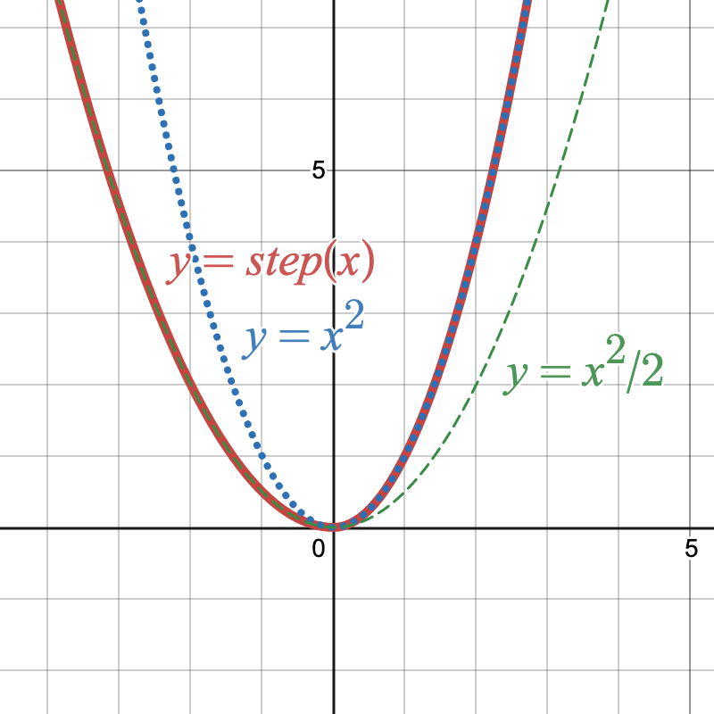
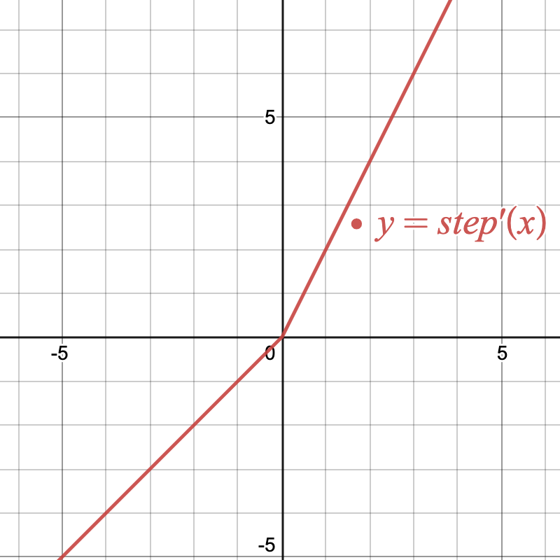
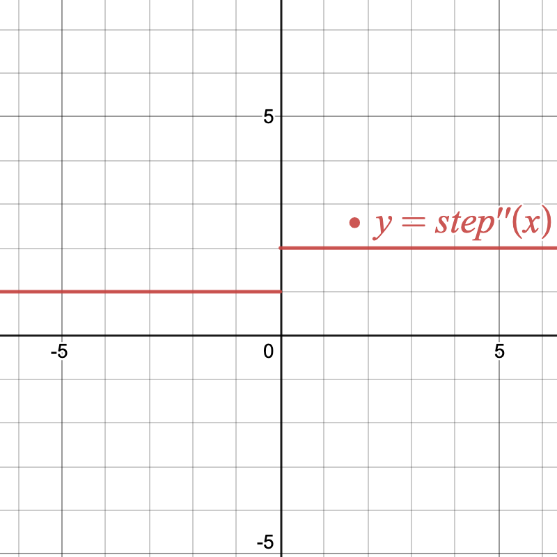
(a)	(b)	(c)

Figure 2: The piecewise quadratic function and its first two derivatives.

Our main technique is comparing the iterates $x^{(0)},x^{(1)},\cdots$ from running SGD on the piecewise quadratic function $f_{1}(x;\xi)$ to the iterates $\{y^{(k)}\}$ and $\{z^{(k)}\}$ obtained from running SGD on the quadratic functions

$$f_{\ell}(x;\xi):=\frac{L}{4}x^{2}+\xi x,\quad\text{and}\quad f_{u}(x;\xi):=\frac{L}{2}x^{2}+\xi x,$$ (B.4)

respectively. We will show in Lemma B.7 that if $x^{(0)}=y^{(0)}=z^{(0)}$, then the iterate $x^{(k)}$ is first-order stochastically dominated by both $y^{(k)}$ and $z^{(k)}$ (see Definition B.6 for the formal definition of first-order stochastic dominance). Fortunately, the iterates $y^{(k)}$ and $z^{(k)}$ are easy to analyze. A straightforward calculation in Lemma B.5 yields the closed form solutions

$$y^{(k)}\sim\alpha_{y}^{k}y^{(0)}+\mathcal{N}(0,\sigma_{y}^{2}),\quad\text{and}\quad z^{(k)}\sim\alpha_{z}^{k}z^{(0)}+\mathcal{N}(0,\sigma_{z}^{2}),$$ (B.5)

where

$$\alpha_{y}:=1-\eta L/2,\quad\alpha_{z}:=1-\eta L,\quad\sigma_{y}^{2}:=\frac{\eta^{2}\sigma^{2}(1-\alpha_{y}^{k})}{1-\alpha_{y}},\quad\sigma_{z}^{2}:=\frac{\eta^{2}\sigma^{2}(1-\alpha_{z}^{k})}{1-\alpha_{z}}.$$ (B.6)

We can then bound the expectation of $x^{(k)}$ in the following way:

$$\mathbb{E}[x^{(k)}]=-\int_{c=-\infty}^{0}{\Pr[x^{(k)}\leq c]}+\int_{c=0}^{\infty}{\Pr[x^{(k)}\geq c]}\leq-\int_{c=-\infty}^{0}{\Pr[y^{(k)}\leq c]}+\int_{c=0}^{\infty}{\Pr[z^{(k)}\geq c]}.$$ (B.7)

This decomposition means that the higher variance of $y^{(k)}$ to contributes to the negative term, while the relatively lower variance of $z^{(k)}$ contributes to the positive term.

To give some intuition, consider the case where $x^{(0)}=y^{(0)}=z^{(0)}=0$, and $\eta Lk\ll 1$. Here we have $y^{(k)}\sim\mathcal{N}(0,\sigma_{y}^{2})$ and $z^{(k)}\sim\mathcal{N}(0,\sigma_{z}^{2})$. Plugging in the cdf of a Gaussian, we obtain

$$\begin{split}-\int_{c=-\infty}^{0}{\Pr[y^{(k)}\leq c]}+\int_{c=0}^{\infty}{\Pr[z^{(k)}\geq c]}=-\frac{\sigma_{y}}{\sqrt{2\pi}}+\frac{\sigma_{z}}{\sqrt{2\pi}}.\end{split}$$

Using the fact that $\eta Lk\ll 1$, we can approximate

$$\sigma_{y}^{2}\approx\frac{\eta^{2}\sigma^{2}(\eta Lk/2+(\eta Lk)^{2}/8)}{\eta L/2}=\eta^{2}\sigma^{2}k(1-\eta Lk/4),$$

and

$$\sigma_{z}^{2}\approx\frac{\eta^{2}\sigma^{2}(\eta Lk/2+(\eta Lk)^{2}/2)}{\eta L}=\eta^{2}\sigma^{2}k(1-\eta Lk/2),$$

such that

$$\mathbb{E}[x^{(k)}]\leq-\frac{\sigma_{y}}{\sqrt{2\pi}}+\frac{\sigma_{z}}{\sqrt{2\pi}}\approx\frac{\eta\sigma\sqrt{k}}{\sqrt{2\pi}}\left(\frac{\eta Lk}{8}\right).$$ (B.8)

When $x^{(0)}$ is non-zero but sufficiently small, we can prove that this same negative iterate bias occurs in the expectation $\mathbb{E}[x^{(k)}]-x^{(0)}$. With slightly more effort, we can show that so long as the expectation $\mathbb{E}[x^{(0)}]$ is sufficiently small, there is a negative drift in $\mathbb{E}[x^{(k)}]-\mathbb{E}[x^{(0)}]$.

We formalize these observations in the following lemma. Note that this lemma also captures the case when $\eta Lk\geq 1$, where $\sigma_{y}-\sigma_{z}=\Theta\left(\sigma\eta^{1/2}L^{-1/2}\right)$.

Lemma B.3.

There exist universal constants $c_{1}$ and $c_{2}$ such that the following holds. Suppose we run SGD with step size $\eta$ on the function $f(x;\xi)=\frac{L}{2}\psi(x)+\xi x$ for $\xi\sim\mathcal{N}(0,\sigma^{2})$ with step size $\eta\leq\frac{1}{6L}$, starting at a possibly random iterate $x^{(0)}$. If

$$-\sqrt{c_{1}}\frac{\sigma_{y}}{\alpha_{y}^{k}}\leq\mathbb{E}[x^{(0)}]\leq 0,$$

then for any $k$,

$$\mathbb{E}[x^{(k)}]\leq\left(1-\eta L/2\right)^{k}\mathbb{E}[x^{(0)}]-\frac{1}{2}c_{2}\sigma\eta^{1/2}L^{-1/2}\min(1,\eta Lk)^{3/2},$$ (B.9)

where $\sigma_{y}$ and $\alpha_{y}$ are defined in Eq. B.6. In particular, we can choose $c_{1}=0.0005$ and $c_{2}=0.002$.

The proof of Lemma B.3 is relegated to Section B.2.

Using Lemma B.3 inductively, we can show that the bias accumulates over many rounds of FedAvg. Loosely speaking, the bias grows linearly with the number of rounds $R$ until the force of the gradient exceeds the drift from the difference $\sigma_{y}-\sigma_{z}$.

Lemma B.4.

Suppose we run FedAvg for $R$ rounds with $K$ local steps and step size $\eta$ on the 1-dimensional function $f(x;\xi)=\frac{L}{2}\psi(x)+\xi x$ for $\xi\sim\mathcal{N}(0,\sigma^{2})$. There exists a universal constant $c$ such that for $\eta\leq\frac{1}{6L}$, if $x^{(0,0)}=0$, then

$$\mathbb{E}[x^{(R,0)}]\leq-c\frac{\sqrt{\eta}\sigma}{\sqrt{L}}\min\left\{R(\eta LK)^{3/2},1,(\eta LK)^{1/2}\right\}$$

In particular, we can choose $c=0.0005$.

The proof of Lemma B.4 is relegated to Section B.3.

Now consider the FedAvg procedure on the 3-dimensional objective $f$ defined in Eq. B.2. Since the trajectories of coordinates of $\mathbf{x}=(x_{1},x_{2},x_{3})$ are completely decoupled, we prove Theorem B.1 by combining Lemma B.4 with bounds that relate the choice of $\eta$ to the suboptimality in the coordinates $x_{2}$ and $x_{3}$. This yields the first term, $O\left(\min\left(\frac{\sigma D}{\sqrt{KR}},\frac{\sigma^{2/3}H^{1/3}D^{4/3}}{K^{1/3}R^{2/3}}\right)\right)$, in Theorem B.1. To obtain the final term, we recall that any first order method which uses at most $MKR$ stochastic gradients has a lower bound of $O(\sigma D/\sqrt{MKR})$ in expected function error. It follows immediately that the function error of FedAvg is at least the maximum these two terms, which is on the same order as their sum. The details of the proof of Theorem B.1 are provided in Section B.5.

B.2 Proof of Lemma B.3

As outlined in the proof overview, we will compare the iterates of SGD on the piecewise quadratic function to the iterates of SGD on quadratic functions. The following lemma gives a closed form for the SGD iterates of a quadratic function.

Lemma B.5 (Distribution of SGD on Quadratic objectives).

Let $x^{(0)}\cdots x^{(t)}$ be the iterates of SGD on the stochastic function $f(x;\xi)=\frac{L}{2}x^{2}+\xi x$ with step size $\eta$ and $\xi\sim\mathcal{N}(0,\sigma^{2})$. Then $x^{(t)}\sim(1-\eta L)^{t}x^{(0)}+\mathcal{N}\left(0,\frac{(1-(1-\eta L)^{t})\eta^{2}\sigma^{2}}{\eta L}\right)$.

Proof of Lemma B.5.

Let $\xi^{(i)}\sim\mathcal{N}(0,\sigma^{2})$, such that

$$x^{(i+1)}=x^{(i)}-\eta(Lx^{(i)}+\xi^{(i)})=(1-\eta L)x^{(i)}-\eta\xi^{(i)}.$$ (B.10)

Recursing, we have

$$\begin{split}x^{(t)}&=(1-\eta L)^{t}x^{(0)}+\sum_{i=1}^{t}\left[(1-\eta L)^{t-i}\eta^{2}\xi^{(i)}\right]\\ &\sim(1-\eta L)^{t}x^{(0)}+\mathcal{N}\left(0,\sum_{i=1}^{t}(1-\eta L)^{t-i}\eta^{2}\sigma^{2}\right)\\ &\sim(1-\eta L)^{t}x^{(0)}+\mathcal{N}\left(0,\frac{(1-(1-\eta L)^{t})\eta^{2}\sigma^{2}}{\eta L}\right).\end{split}$$

∎

We introduce the following definition to facilitate the proof.

Definition B.6.

A random variable $Y$ first-order stochastically dominates a random variable $X$ if for all values $c\in\mathbb{R}$,

$$\Pr[Y\geq c]\geq\Pr[X\geq c].$$ (B.11)

We will use the following lemma.

Lemma B.7 (Markov Chain Stochastic Dominance).

Let $X_{t}$ and $Y_{t}$ be time-homogeneous discrete-time Markov chains on $\mathbb{R}$ such that for any $z$, the random variable $Y_{1}|Y_{0}=z$ first-order stochastically dominates $X_{1}|X_{0}=z$. Then for any $c$ and any $t>0$, $Y_{t}|Y_{0}=c$ first-order stochastically dominates $X_{t}|X_{0}=c$.

Proof of Lemma B.7.

We prove this by induction on $t$. Note that it holds trivially for $t=0$.

Let $p_{x}$ be the distribution of $X_{t-1}|X_{0}=c$ and $p_{y}$ be the distribution of $Y_{t-1}|Y_{0}=c$, such that by our inductive hypothesis, $p_{y}$ stochastically dominates $p_{x}$.

Then for any $c$, we have

$$\begin{split}\Pr[Y_{t}\geq c|Y_{t-1}\sim p_{y}]&=\Pr[Y_{1}\geq c|Y_{0}\sim p_{y}]\\ &\geq\Pr[X_{1}\geq c|X_{0}\sim p_{y}]\\ &\geq\Pr[X_{1}\geq c|X_{0}\sim p_{x}]\\ &=\Pr[X_{t}\geq c|X_{t-1}\sim p_{x}].\end{split}$$

Here the equalities follow from the fact that $X_{t}$ and $Y_{t}$ are Markov chains. The first inequality follows from our assumption that for any $z$, $Y_{1}|Y_{0}=z$ first-order stochastically dominates $X_{1}|X_{0}=z$. The second inequality follows from the fact that the function $f(z):=\Pr[X_{1}\leq c|X_{0}=z]$ is increasing in $z$, so its expectation is at least as large under $z\sim p_{y}$ as under $z\sim p_{x}$. ∎

Lemma B.3, the more general form of Lemma 3.4, gives the bias of SGD on the piecewise quadratic function if the expectation of the starting iterate is bounded. The most important part of its proof is the following weaker lemma, which gives the bias is SGD if the first iterate is deterministic and bounded.

Recall the variables introduced in the proof overview Eq. B.6, which we restate here for ease of reference:

$$\alpha_{y}:=1-\eta L/2,\quad\alpha_{z}:=1-\eta L,\quad\sigma_{y}^{2}:=\frac{\eta^{2}\sigma^{2}(1-\alpha_{y}^{k})}{1-\alpha_{y}},\quad\sigma_{z}^{2}:=\frac{\eta^{2}\sigma^{2}(1-\alpha_{z}^{k})}{1-\alpha_{z}}.$$ (B.12)

Lemma B.8.

If $\eta L\leq 1/6$ and

$$-\sqrt{c_{1}}\frac{\sigma_{y}}{\alpha_{y}^{k}}\leq x^{(0)}\leq\sqrt{c_{1}}\frac{\sigma_{y}}{\alpha_{y}^{k}},$$ (B.13)

then

$$\mathbb{E}[x^{(k)}|x^{(0)}]\leq\max\left\{\left(1-\eta L\right)^{k}x^{(0)},\left(1-\eta L/2\right)^{k}x^{(0)}\right\}-c_{2}\frac{\sigma\sqrt{\eta}}{\sqrt{L}}\min\left(\eta Lk,1\right)^{3/2},$$ (B.14)

where $c_{1}=0.0005$ and $c_{2}=0.002$.

The proof of Lemma B.8 is deferred to Section B.2.1.

The following lemma covers the edge cases when $|x^{(0)}|$ is large.

Lemma B.9.

For all $x^{(0)}\in\mathbb{R}$,

$$\mathbb{E}[x^{(k)}|x^{(0)}]\leq\left(1-\eta L\right)^{k}x^{(0)},$$ (B.15)

and

$$\mathbb{E}[x^{(k)}|x^{(0)}]\leq\left(1-\frac{\eta L}{2}\right)^{k}x^{(0)}.$$ (B.16)

We begin by proving Lemma B.9.

Proof of Lemma B.9.

This follows immediately from Lemma B.7, since $x^{(k)}$ is stochastically dominated by $k$ steps the SGD processes $y^{(k)}$ and $z^{(k)}$ on the functions $f_{\ell}(x,\xi):=\frac{L}{4}x^{2}+\xi x$ and $f_{u}(x;\xi):=\frac{L}{2}x^{2}+\xi x$ respectively, with $y^{(0)}=z^{(0)}=x^{(0)}$. Indeed by Lemma B.5,

$$\mathbb{E}[x^{(k)}]\leq\mathbb{E}[z^{(k)}]=\left(1-\eta L\right)^{k}x^{(0)},$$

and

$$\mathbb{E}[x^{(k)}]\leq\mathbb{E}[y^{(k)}]=\left(1-\frac{\eta L}{2}\right)^{k}x^{(0)}.$$

∎

We now prove Lemma B.3 from Lemmas B.8 and B.9.

Proof of Lemma B.3.

We divide the proof into two cases. Let $B:=\sqrt{c_{1}}\frac{\sigma_{y}}{\alpha_{y}^{k}}$ and let $\delta:=c_{2}\sigma\eta^{1/2}L^{-1/2}\min(1,\eta Lk)^{3/2}$.

Case 1: $\Pr[-B\leq x^{(0)}\leq B]\geq\frac{1}{2}$. In this case, using the second statement of Lemma B.9 in the first inequality and Lemma B.8 in the second inequality, we achieve

$$\begin{split}\mathbb{E}[x^{(k)}]&=\Pr[|x^{(0)}|\geq B]\mathbb{E}[x^{(k)}\mid|x^{(0)}|\geq B]+\Pr[|x^{(0)}|\leq B]\mathbb{E}\left[x^{(k)}\middle||x^{(0)}|\leq B\right]\\ &\leq\Pr[|x^{(0)}|\geq B]\mathbb{E}[\left(1-\eta L/2\right)^{k}x^{(0)}\mid|x^{(0)}|\geq B]+\Pr[|x^{(0)}|\leq B]\mathbb{E}\left[x^{(k)}\middle||x^{(0)}|\leq B\right]\\ &\leq\Pr[|x^{(0)}|\geq B]\mathbb{E}[\left(1-\eta L/2\right)^{k}x^{(0)}\mid|x^{(0)}|\geq B]+\Pr[|x^{(0)}|\leq B]\mathbb{E}[\left(1-\eta L\right)^{k}x^{(0)}-\delta\mid|x^{(0)}|\leq B]\\ &=\left(1-\eta L/2\right)^{k}\mathbb{E}[x^{(0)}]-\delta\Pr[|x^{(0)}|\leq B]\\ &\leq\left(1-\eta L/2\right)^{k}\mathbb{E}[x^{(0)}]-\frac{\delta}{2}.\end{split}$$

This gives the desired result.

Case 2: $\Pr[-B\leq x^{(0)}\leq B]\leq\frac{1}{2}$. In this case, using the first statement of Lemmas B.9 in the first inequality, and the second statement of Lemma B.9 in the second inequality, we have

$$\begin{split}\mathbb{E}[x^{(k)}]&=\Pr[x^{(0)}\leq B]\mathbb{E}[x^{(k)}\mid x^{(0)}\leq B]+\Pr[x^{(0)}>B]\mathbb{E}[x^{(k)}\mid x^{(0)}>B]\\ &\leq\Pr[x^{(0)}\leq B]\mathbb{E}\left[\left(1-\frac{\eta L}{2}\right)^{k}x^{(0)}\mid x^{(0)}\leq B\right]+\Pr[x^{(0)}>B]\mathbb{E}\left[x^{(k)}\mid x^{(0)}>B\right]\\ &\leq\Pr[x^{(0)}\leq B]\mathbb{E}\left[\left(1-\frac{\eta L}{2}\right)^{k}x^{(0)}\mid x^{(0)}\leq B\right]+\Pr[x^{(0)}>B]\mathbb{E}\left[\left(1-\eta L\right)^{k}x^{(0)}\mid x^{(0)}>B\right]\\ &=\left(1-\frac{\eta L}{2}\right)^{k}\mathbb{E}[x^{(0)}]+\Pr[x^{(0)}>B]\mathbb{E}\left[\left(\left(1-\eta L\right)^{k}-\left(1-\frac{\eta L}{2}\right)^{k}\right)x^{(0)}\mid x^{(0)}>B\right].\\ \end{split}$$

Now

$$\begin{split}(1-\eta L/2)^{k}-(1-\eta L)^{k}&\geq\begin{cases}1-\eta Lk/2-(1-\eta Lk+(\eta Lk)^{2}/2)&\eta Lk\leq 1/2;\\ \alpha_{y}^{k}\left(1-(1-\eta L/2)^{k}\right)&\eta Lk\geq 1/2,\end{cases}\\ &\geq\begin{cases}\eta Lk/4&\eta Lk\leq 1/2;\\ \alpha_{y}^{k}(1-e^{-\eta Lk/2})&\eta Lk\geq 1/2.\end{cases}\\ &\geq\begin{cases}\eta Lk/4&\eta Lk\leq 1/2;\\ \frac{\alpha_{y}^{k}}{5}&\eta Lk\geq 1/2.\end{cases}\\ \end{split}$$

Plugging this in to the previous equation, it follows that

$$\mathbb{E}[x^{(k)}]\leq\left(1-\frac{\eta L}{2}\right)^{k}\mathbb{E}[x^{(0)}]+\begin{cases}\Pr[x^{(0)}>B]\mathbb{E}[x^{(0)}|x^{(0)}\geq B]\frac{\eta Lk}{4}&\eta Lk\leq 1/2;\\ \Pr[x^{(0)}>B]\mathbb{E}[x^{(0)}|x^{(0)}\geq B]\frac{\alpha_{y}^{k}}{5}&\eta Lk\geq 1/2.\end{cases}$$ (B.17)

Now we can bound

$$\begin{split}\Pr[x^{(0)}>B]\mathbb{E}\left[x^{(0)}\mid x^{(0)}>B\right]&=\mathbb{E}[x^{(0)}]-\Pr[|x^{(0)}|\leq B]\mathbb{E}\left[x^{(0)}\mid|x^{(0)}|\leq B\right]-\Pr[x^{(0)}<-B]\mathbb{E}\left[x^{(0)}\mid x^{(0)}<-B\right]\\ &\geq\mathbb{E}[x^{(0)}]-\frac{1}{2}\left(B\right)-0\geq B-\frac{B}{2}\geq\frac{B}{2}.\end{split}$$

Plugging this calculation into the result of Equation B.17 yields

$$\begin{split}\mathbb{E}[x^{(k)}]&\leq\left(1-\eta L/2\right)^{k}\mathbb{E}[x^{(0)}]-\begin{cases}\frac{\sqrt{c_{1}}}{2}\frac{\sigma_{y}}{\alpha_{y}^{k}}\frac{\eta Lk}{4}&\eta Lk\leq 1/2\\ \frac{\sqrt{c_{1}}}{2}\frac{\sigma_{y}}{\alpha_{y}^{k}}\frac{\alpha_{y}^{k}}{5}&\eta Lk\geq 1/2\end{cases}\\ &\leq\left(1-\eta L/2\right)^{k}\mathbb{E}[x^{(0)}]-\begin{cases}\frac{\sqrt{c_{1}}}{2}\frac{\eta\sigma\sqrt{k}}{2}\frac{\eta Lk}{4}&\eta Lk\leq 1/2\\ \frac{\sqrt{c_{1}}}{2}\sigma_{y}\frac{1}{5}&\eta Lk\geq 1/2\end{cases}\\ &\leq\left(1-\eta L/2\right)^{k}\mathbb{E}[x^{(0)}]-\begin{cases}\frac{\sqrt{c_{1}}}{2}\frac{\eta\sigma\sqrt{k}}{2}\frac{\eta Lk}{4}&\eta Lk\leq 1/2\\ \frac{\sqrt{c_{1}}}{2}\frac{2\sqrt{\eta}\sigma}{\sqrt{L}}\frac{1}{5}&\eta Lk\geq 1/2\end{cases}\\ &\leq\left(1-\eta L/2\right)^{k}\mathbb{E}[x^{(0)}]-\begin{cases}\frac{\sqrt{c_{1}}}{16c_{2}}\delta&\eta Lk\leq 1/2\\ \frac{\sqrt{c_{1}}}{5c_{2}}\delta&\eta Lk\geq 1/2\end{cases}\\ &\leq\left(1-\eta L/2\right)^{k}\mathbb{E}[x^{(0)}]-\frac{\delta}{2}.\end{split}$$

This proves the lemma. ∎

B.2.1 Deferred proof of Lemma B.8

Proof of Lemma B.8.

Let $f_{\ell}(x,\xi):=\frac{L}{4}x^{2}+\xi x$ and $f_{u}(x,\xi):=\frac{L}{2}x^{2}+\xi x$. Let $y^{(k)}$ be the iterates of SGD on $f_{\ell}$ and let $z^{(k)}$ be the iterates of SGD on $f_{u}$, both initialized at $y^{(0)}=z^{(0)}=x^{(0)}$, with $\xi\sim\mathcal{N}(0,\sigma^{2})$.

Then by Lemma B.7,

$$\begin{split}\mathbb{E}[x^{(k)}]&=-\int_{c=-\infty}^{0}{\Pr[x^{(k)}\leq c]}+\int_{c=0}^{\infty}{\Pr[x^{(k)}\geq c]}\leq-\int_{c=-\infty}^{0}{\Pr[y^{(k)}\leq c]}+\int_{c=0}^{\infty}{\Pr[z^{(k)}\geq c]}\\ \end{split}$$

By Lemma B.5, we have

$$y^{(k)}\sim\alpha_{y}^{k}x^{(0)}+\mathcal{N}\left(0,\frac{(1-\alpha_{y}^{k})\eta^{2}\sigma^{2}}{1-\alpha_{y}}\right),\quad\text{and}\quad z^{(k)}\sim\alpha_{z}^{k}x^{(0)}+\mathcal{N}\left(0,\frac{(1-\alpha_{z}^{k})\eta^{2}\sigma^{2}}{1-\alpha_{z}}\right).$$

Now with $Y\sim\mathcal{N}\left(0,\sigma^{2}_{y}\right)$ for $\sigma^{2}_{y}=\frac{(1-\alpha_{y}^{k})\eta^{2}\sigma^{2}}{1-\alpha_{y}}$, we have

$$\begin{split}\Pr[y^{(k)}\leq c]=\Pr\left[Y\leq c-\alpha_{y}^{k}x^{(0)}\right],\end{split}$$

so

$$\begin{split}\int_{c=-\infty}^{0}\Pr\left[Y\leq c-\alpha_{y}^{k}x^{(0)}\right]&=\mathbb{E}\left[-\alpha_{y}^{k}x^{(0)}-Y|Y\leq-\alpha_{y}^{k}x^{(0)}\right]\Pr\left[Y\leq-\alpha_{y}^{k}x^{(0)}\right]\\ &=\left(-\alpha_{y}^{k}x^{(0)}-\mathbb{E}\left[Y|Y\leq-\alpha_{y}^{k}x^{(0)}\right]\right)\Pr\left[Y\leq-\alpha_{y}^{k}x^{(0)}\right].\end{split}$$

Now for any $a$,

$$\mathbb{E}[Y|Y\leq a]\Pr[Y\leq a]=\frac{1}{\sigma_{y}\sqrt{2\pi}}\int_{t=-\infty}^{a}te^{-\frac{t^{2}}{2\sigma_{y}^{2}}}dt=-\frac{\sigma_{y}^{2}}{\sigma_{y}\sqrt{2\pi}}e^{-\frac{t^{2}}{2\sigma_{y}^{2}}}\Bigg{|}_{t=-\infty}^{t=a}=-\sigma_{y}\frac{e^{-\frac{a^{2}}{2\sigma^{2}_{y}}}}{\sqrt{2\pi}}.$$ (B.18)

Hence we have

$$\int_{c=-\infty}^{0}{\Pr[y^{(k)}\leq c]}=-\alpha_{y}^{k}x^{(0)}\Pr\left[\mathcal{N}(0,\sigma_{y}^{2})\leq-a_{y}^{k}x^{(0)}\right]+\sigma_{y}\frac{e^{-\frac{(\alpha_{y}^{k}x^{(0)})^{2}}{2\sigma_{y}}}}{\sqrt{2\pi}}.$$ (B.19)

Similarly, with $Z\sim\mathcal{N}\left(0,\sigma_{z}^{2}\right)$ with $\sigma_{z}^{2}=\frac{(1-\alpha_{z}^{k})\eta^{2}\sigma^{2}}{1-\alpha_{z}}$, we have

$$\begin{split}\int_{c=0}^{\infty}{\Pr[z^{(k)}\geq c]}&=\mathbb{E}\left[Z+\alpha_{z}^{k}x^{(0)}|Z\geq-\alpha_{z}^{k}x^{(0)}\right]\Pr\left[Z\geq-\alpha_{z}^{k}x^{(0)}\right]\\ &=\left(\alpha_{z}^{k}x^{(0)}+\mathbb{E}\left[Z|Z\geq-\alpha_{z}^{k}x^{(0)}\right]\right)\Pr\left[Z\geq-\alpha_{z}^{k}x^{(0)}\right]\\ &=\alpha_{z}^{k}x^{(0)}\Pr\left[\mathcal{N}(0,\sigma_{z}^{2})\geq-\alpha_{z}^{k}x^{(0)}\right]+\sigma_{z}\frac{e^{-\frac{(\alpha_{z}^{k}x^{(0)})^{2}}{2\sigma_{z}}}}{\sqrt{2\pi}}.\end{split}$$

Summing, we have

$$\begin{split}\mathbb{E}[x^{(k)}]&=x^{(0)}\left(\alpha_{z}^{k}\Pr\left[\mathcal{N}(0,\sigma_{z}^{2})\geq-\alpha_{z}^{k}x^{(0)}\right]+\alpha_{y}^{k}\Pr\left[\mathcal{N}(0,\sigma_{y}^{2})\leq-\alpha_{y}^{k}x^{(0)}\right]\right)\\ &\qquad+\sigma_{z}\frac{e^{-\frac{(\alpha_{z}^{k}x^{(0)})^{2}}{2\sigma^{2}_{z}}}}{\sqrt{2\pi}}-\sigma_{y}\frac{e^{-\frac{(\alpha_{y}^{k}x^{(0)})^{2}}{2\sigma_{y}^{2}}}}{\sqrt{2\pi}}\end{split}$$

We bound the terms in Equation B.2.1 with the following three claims. The proofs of Claims B.10, B.11 and B.12 are deferred to the end of the present subsubsection.

Claim B.10.

$$\sigma_{z}\frac{e^{-\frac{(\alpha_{z}^{k}x^{(0)})^{2}}{2\sigma^{2}_{z}}}}{\sqrt{2\pi}}-\sigma_{y}\frac{e^{-\frac{(\alpha_{y}^{k}x^{(0)})^{2}}{2\sigma_{y}^{2}}}}{\sqrt{2\pi}}\leq\frac{\sigma_{z}-\sigma_{y}}{\sqrt{2\pi}}\left(e^{-c_{1}}\right)+\begin{cases}c_{1}\eta^{2}\sigma Lk^{3/2}&\eta Lk\leq 1/2;\\ \frac{\eta^{1/2}\sigma c_{1}}{L^{1/2}\sqrt{2\pi}}&\eta Lk\geq 1/2.\end{cases}$$ (B.20)

Claim B.11.

$$\begin{split}x^{(0)}&\left(\alpha_{z}^{k}\Pr\left[\mathcal{N}(0,\sigma_{z}^{2})\geq-\alpha_{z}^{k}x^{(0)}\right]+\alpha_{y}^{k}\Pr\left[\mathcal{N}(0,\sigma_{y}^{2})\leq-\alpha_{y}^{k}x^{(0)}\right]\right)\\ &\leq x^{(0)}\alpha_{y}^{k}+c_{1}\left(\sigma_{y}-\sigma_{x}\right)+\begin{cases}\sqrt{c_{1}}\eta^{2}\sigma Lk^{3/2}&\eta Lk\leq 1/2;\\ \frac{\sqrt{c_{1}}}{2}\frac{\sqrt{\eta}\sigma}{\sqrt{L}}&\eta Lk\geq 1/2.\end{cases}\end{split}$$

Claim B.12.

$$\sigma_{y}-\sigma_{z}\geq\begin{cases}\frac{1}{24}\eta^{2}L\sigma k^{3/2}&\eta Lk\leq 1/2;\\ \frac{0.12\eta\sigma}{\sqrt{\eta L}}&\eta Lk\geq 1/2.\end{cases}$$ (B.21)

Combining the results of Claims B.10 and B.11 with Equation B.2.1, we obtain

$$\begin{split}\mathbb{E}[x^{(k)}]&\leq x^{(0)}\alpha_{y}^{k}+\left(\sigma_{z}-\sigma_{y}\right)\left(\frac{e^{-c_{1}}}{\sqrt{2\pi}}-c_{1}\right)+\begin{cases}(c_{1}+\sqrt{c_{1}}/2)\eta^{2}\sigma Lk^{3/2}&\eta Lk\leq 1/2;\\ \frac{\sqrt{\eta}\sigma}{\sqrt{L}}\left(\frac{c_{1}}{\sqrt{2\pi}}+2\sqrt{c_{1}}\right)&\eta Lk\geq 1/2.\end{cases}\\ \end{split}$$

Plugging in Claim B.12, we obtain for $c_{1}\leq 0.0005$,

$$\begin{split}\mathbb{E}[x^{(k)}]&\leq x^{(0)}\alpha_{y}^{k}+\begin{cases}-\left(\frac{e^{-c_{1}}}{\sqrt{2\pi}}-c_{1}\right)\left(\frac{1}{24}\eta^{2}L\sigma k^{3/2}\right)+(c_{1}+\sqrt{c_{1}}/2)\eta^{2}\sigma Lk^{3/2}&\eta Lk\leq 1/2;\\ -\left(\frac{e^{-c_{1}}}{\sqrt{2\pi}}-c_{1}\right)\left(\frac{0.12\sqrt{\eta}\sigma}{\sqrt{L}}\right)+\frac{\sqrt{\eta}\sigma}{\sqrt{L}}\left(\frac{c_{1}}{\sqrt{2\pi}}+2\sqrt{c_{1}}\right)&\eta Lk\geq 1/2.\end{cases}\\ &=x^{(0)}\alpha_{y}^{k}+\begin{cases}-\left(\frac{e^{-c_{1}}}{\sqrt{2\pi}}-c_{1}-24c_{1}-12\sqrt{c_{1}}\right)\left(\frac{1}{24}\eta^{2}L\sigma k^{3/2}\right)&\eta Lk\leq 1/2;\\ -\left(\frac{e^{-c_{1}}}{\sqrt{2\pi}}-c_{1}-\frac{c_{1}}{0.12\sqrt{2\pi}}-\frac{2\sqrt{c_{1}}}{0.12}\right)\left(\frac{0.12\sqrt{\eta}\sigma}{\sqrt{L}}\right)&\eta Lk\geq 1/2.\end{cases}\\ &\leq x^{(0)}\alpha_{y}^{k}+\begin{cases}-0.117\left(\frac{1}{24}\eta^{2}L\sigma k^{3/2}\right)&\eta Lk\leq 1/2;\\ -0.023\left(\frac{0.12\sqrt{\eta}\sigma}{\sqrt{L}}\right)&\eta Lk\geq 1/2.\end{cases}\\ &\leq x^{(0)}\alpha_{y}^{k}-\frac{0.002\sqrt{\eta}\sigma\min(\eta Lk,1)^{3/2}}{\sqrt{L}}.\end{split}$$

This concludes the proof of the lemma aside from the proof of the three claims. To prove these, observe that $\alpha_{z}\leq\alpha_{y}$, and $\sigma_{z}\leq\sigma_{y}$. ∎

Deferred Proof of Claim B.10.

$$\begin{split}\sigma_{z}\frac{e^{-\frac{(\alpha_{z}^{k}x^{(0)})^{2}}{2\sigma^{2}_{z}}}}{\sqrt{2\pi}}-\sigma_{y}\frac{e^{-\frac{(\alpha_{y}^{k}x^{(0)})^{2}}{2\sigma_{y}^{2}}}}{\sqrt{2\pi}}&=\frac{\sigma_{z}-\sigma_{y}}{\sqrt{2\pi}}\left(e^{-\frac{(\alpha_{z}^{k}x^{(0)})^{2}}{2\sigma^{2}_{z}}}\right)+\frac{\sigma_{y}}{\sqrt{2\pi}}\left(e^{-\frac{(\alpha_{z}^{k}x^{(0)})^{2}}{2\sigma^{2}_{z}}}-e^{-\frac{(\alpha_{y}^{k}x^{(0)})^{2}}{2\sigma_{y}^{2}}}\right)\\ &\leq\frac{\sigma_{z}-\sigma_{y}}{\sqrt{2\pi}}\left(e^{-c_{1}/2}\right)+\frac{\sigma_{y}}{\sqrt{2\pi}}\left(e^{-\frac{(\alpha_{z}^{k}x^{(0)})^{2}}{2\sigma^{2}_{z}}}-e^{-\frac{(\alpha_{y}^{k}x^{(0)})^{2}}{2\sigma_{y}^{2}}}\right)\\ &\leq\frac{\sigma_{z}-\sigma_{y}}{\sqrt{2\pi}}\left(e^{-c_{1}/2}\right)+\frac{\sigma_{y}}{\sqrt{2\pi}}\left|\frac{(\alpha_{z}^{k}x^{(0)})^{2}}{2\sigma^{2}_{z}}-\frac{(\alpha_{y}^{k}x^{(0)})^{2}}{2\sigma_{y}^{2}}\right|\max\left(e^{-\frac{(\alpha_{z}^{k}x^{(0)})^{2}}{2\sigma^{2}_{z}}},e^{-\frac{(\alpha_{y}^{k}x^{(0)})^{2}}{2\sigma_{y}^{2}}}\right)\\ &\leq\frac{\sigma_{z}-\sigma_{y}}{\sqrt{2\pi}}\left(e^{-c_{1}/2}\right)+\frac{\sigma_{y}}{\sqrt{2\pi}}\left|\frac{(\alpha_{z}^{k}x^{(0)})^{2}}{2\sigma^{2}_{z}}-\frac{(\alpha_{y}^{k}x^{(0)})^{2}}{2\sigma_{y}^{2}}\right|\\ &=\frac{\sigma_{z}-\sigma_{y}}{\sqrt{2\pi}}\left(e^{-c_{1}/2}\right)+\frac{\sigma_{y}(x^{(0)})^{2}}{2\sqrt{2\pi}}\left|\frac{\alpha_{z}^{2k}}{\sigma^{2}_{z}}-\frac{\alpha_{y}^{2k}}{\sigma_{y}^{2}}\right|\\ &\leq\frac{\sigma_{z}-\sigma_{y}}{\sqrt{2\pi}}\left(e^{-c_{1}/2}\right)+\frac{\sigma_{y}(x^{(0)})^{2}}{2\sqrt{2\pi}}\left|\frac{\alpha_{z}^{2k}-\alpha_{y}^{2k}}{\sigma_{y}^{2}}\right|.\\ \end{split}$$

By the assumption on $(x^{(0)})^{2}$ in the lemma, we have

$$\frac{\sigma_{y}(x^{(0)})^{2}}{2\sqrt{2\pi}}\left|\frac{\alpha_{z}^{2k}-\alpha_{y}^{2k}}{\sigma_{y}^{2}}\right|\leq\frac{\sigma_{y}(x^{(0)})^{2}}{2\sqrt{2\pi}}\frac{\alpha_{y}^{2k}}{\sigma_{y}^{2}}\leq\frac{\sigma_{y}c_{1}}{2\sqrt{2\pi}}\leq\frac{\sqrt{\eta}\sigma c_{1}}{\sqrt{L}\sqrt{2\pi}}.$$ (B.22)

Now if $\eta Lk\leq 1/2$,

$$\begin{split}\frac{\sigma_{y}(x^{(0)})^{2}}{2\sqrt{2\pi}}\left|\frac{\alpha_{z}^{2k}-\alpha_{y}^{2k}}{\sigma_{y}^{2}}\right|&=\frac{(x^{(0)})^{2}\alpha_{y}^{2k}}{2\sigma_{y}\sqrt{2\pi}}\left|\left(\frac{(1-\eta L)}{(1-\eta L/2)}\right)^{2k}-1\right|\\ &=\frac{(x^{(0)})^{2}\alpha_{y}^{2k}}{2\sigma_{y}\sqrt{2\pi}}\left|\left(1-\eta L\right)^{2k}-1\right|\\ &\leq\frac{(x^{(0)})^{2}\alpha_{y}^{2k}}{2\sigma_{y}\sqrt{2\pi}}\left(2\eta Lk\right)\\ &\leq\sigma_{y}c_{1}\eta Lk,\\ &=\left(\sqrt{\frac{(1-(1-\eta L/2)^{k})\eta^{2}\sigma^{2}}{\eta L/2}}\right)c_{1}\eta Lk\\ &\leq\left(\eta\sigma\frac{1-(1-\eta Lk/2)}{\eta L/2}\right)c_{1}\eta Lk\\ &=c_{1}\eta^{2}\sigma Lk^{3/2}.\end{split}$$

Here in the second inequality we used the condition on $(x^{(0)})^{2}$. This proves the claim. ∎

Deferred Proof of Claim B.11.

Observe that

$$\begin{split}x^{(0)}\Pr\left[\mathcal{N}(0,\sigma_{z}^{2})\geq-\alpha_{z}^{k}x^{(0)}\right]\leq x^{(0)}\Pr\left[\mathcal{N}(0,\sigma_{z}^{2})\geq-\alpha_{y}^{k}x^{(0)}\right]\end{split}$$

and

$$\begin{split}\alpha_{y}^{k}x^{(0)}\Pr\left[\mathcal{N}(0,\sigma_{y}^{2})\leq-\alpha_{y}^{k}x^{(0)}\right]&=\alpha_{y}^{k}x^{(0)}\Pr\left[\mathcal{N}(0,\sigma_{z}^{2})\leq-\alpha_{y}^{k}x^{(0)}\right]-\alpha_{y}^{k}x^{(0)}\int_{c=-\alpha_{y}^{k}x^{(0)}}^{0}{\mu_{\sigma_{z}}(c)-\mu_{\sigma_{y}}(c)}dc\\ &\leq\alpha_{y}^{k}x^{(0)}\Pr\left[\mathcal{N}(0,\sigma_{z}^{2})\leq-\alpha_{y}^{k}x^{(0)}\right]+\alpha_{y}^{2k}(x^{(0)})^{2}\max_{-\infty\leq c\leq\infty}\left|\mu_{\sigma_{z}}(c)-\mu_{\sigma_{y}}(c)\right|,\end{split}$$

as shown in Figure 3.

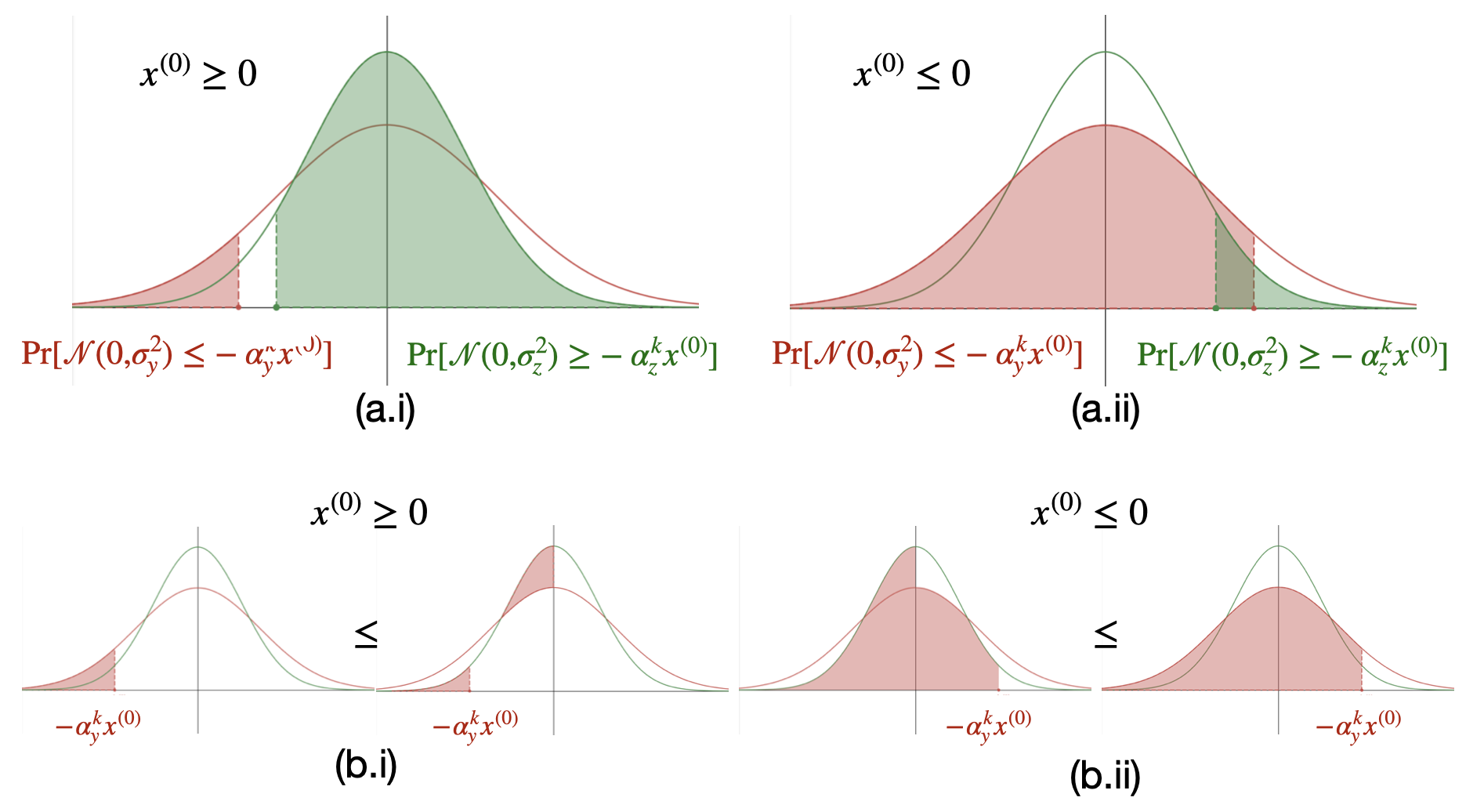
Figure 3: Comparison of CDFs. (a) and (b): the regions in the first line of Equation B.2.1 for positive (a.i) or negative $x^{(0)}$ (a.ii). (b) The inequality used in Equation B.2.1 for both positive (b.i) or negative $x^{(0)}$ (b.ii). In each of (b.i) and (b.ii), the shaded region on the right is larger than the shaded region on the left.

Now

$$\begin{split}\max_{-\infty\leq c\leq\infty}\left|\frac{1}{\sqrt{2\pi\sigma_{z}^{2}}}e^{-c^{2}/(2\sigma_{z}^{2})}-\frac{1}{\sqrt{2\pi\sigma_{y}^{2}}}e^{-c^{2}/(2\sigma_{y}^{2})}\right|&=\left(\frac{1}{\sqrt{2\pi\sigma_{z}^{2}}}-\frac{1}{\sqrt{2\pi\sigma_{y}^{2}}}\right)\\ &=\left(\frac{1}{\sqrt{2\pi\sigma_{z}^{2}}}\left(1-\frac{1}{\sqrt{1+(\sigma_{y}^{2}-\sigma_{z}^{2})/\sigma_{z}^{2}}}\right)\right)\\ &\leq\left(\frac{1}{\sqrt{2\pi\sigma_{z}^{2}}}\frac{\sigma_{y}^{2}-\sigma_{z}^{2}}{2\sigma_{z}^{2}}\right)\\ &=\left(\frac{(\sigma_{y}-\sigma_{z})\sigma_{y}}{2\sigma^{2}_{z}\sqrt{2\pi\sigma_{z}^{2}}}\right)\end{split}$$

To bound this term, observe that

$$\frac{\sigma_{y}^{2}}{\sigma_{z}^{2}}=\frac{(1-\alpha_{y}^{k})(1-\alpha_{z})}{(1-\alpha_{z}^{k})(1-\alpha_{y})}=2\frac{(1-\alpha_{y}^{k})}{(1-\alpha_{z}^{k})}\leq 2,$$ (B.23)

so

$$\alpha_{y}^{2k}(x^{(0)})^{2}\frac{\sigma_{y}(\sigma_{y}-\sigma_{z})}{2\sigma_{z}^{2}\sqrt{2\pi\sigma_{z}^{2}}} \leq\frac{\alpha_{y}^{k}(x^{(0)})^{2}}{\sigma_{y}^{2}}\frac{\sigma_{y}(\sigma_{y}-\sigma_{z})}{\sqrt{2\pi\sigma_{z}^{2}}} \sigma_{y}^{2}\leq 2\sigma_{z}^{2}$$ ()

$$\leq c_{1}\frac{\sigma_{y}(\sigma_{y}-\sigma_{z})}{\sqrt{2\pi\sigma_{z}^{2}}} (x^{(0)})^{2}\leq\frac{\sigma_{y}^{2}}{\alpha_{y}^{2k}}$$ ()

$$\leq c_{1}\left(\sigma_{y}-\sigma_{z}\right). \sigma_{y}^{2}\leq 2\sigma_{z}^{2}$$ ()

Plugging Equation B.2.1 into Equation B.2.1, and then plugging in this last equation, we obtain

$$\alpha_{y}^{k}x^{(0)}\Pr\left[\mathcal{N}(0,\sigma_{y}^{2})\leq-\alpha_{y}^{k}x^{(0)}\right]\leq\alpha_{y}^{k}x^{(0)}\Pr\left[\mathcal{N}(0,\sigma_{z}^{2})\leq-\alpha_{y}^{k}x^{(0)}\right]+c_{1}\left(\sigma_{y}-\sigma_{x}\right).$$ (B.24)

We combine Equations B.11 with B.24 to yield

$$\begin{split}x^{(0)}&\left(\alpha_{z}^{k}\Pr\left[\mathcal{N}(0,\sigma_{z}^{2})\geq-\alpha_{z}^{k}x^{(0)}\right]+\alpha_{y}^{k}\Pr\left[\mathcal{N}(0,\sigma_{y}^{2})\leq-\alpha_{y}^{k}x^{(0)}\right]\right)\\ &\leq x^{(0)}\left(\alpha_{z}^{k}\Pr\left[\mathcal{N}(0,\sigma_{z}^{2})\geq-\alpha_{y}^{k}x^{(0)}\right]+\alpha_{y}^{k}\Pr\left[\mathcal{N}(0,\sigma_{z}^{2})\leq-\alpha_{y}^{k}x^{(0)}\right]\right)+c_{1}\left(\sigma_{y}-\sigma_{x}\right)\\ &\leq\max(x^{(0)}\alpha_{y}^{k},x^{(0)}\alpha_{z}^{k})+c_{1}\left(\sigma_{y}-\sigma_{x}\right).\end{split}$$

Now by similar calculations as in Equation B.22 and B.2.1, we have

$$\begin{split}\max(x^{(0)}\alpha_{y}^{k},x^{(0)}\alpha_{z}^{k})&\leq x^{(0)}\alpha_{y}^{k}+(\alpha_{y}^{k}-\alpha_{z}^{k})|x^{(0)}|\\ &\leq x^{(0)}\alpha_{y}^{k}+\begin{cases}\sqrt{c_{1}}\sigma_{y}\frac{\eta Lk}{2}&\eta Lk\leq 1/2;\\ \sqrt{c_{1}}\sigma_{y}&\eta Lk\geq 1/2.\end{cases}\\ &\leq x^{(0)}\alpha_{y}^{k}+\begin{cases}\frac{\sqrt{c_{1}}}{2}\eta^{2}\sigma Lk^{3/2}&\eta Lk\leq 1/2;\\ \sqrt{c_{1}}\frac{2\sqrt{\eta}\sigma}{\sqrt{L}}&\eta Lk\geq 1/2.\end{cases}\\ \end{split}$$

Plugging this in to the previous equation concludes the proof of the claim. ∎

Deferred Proof of Claim B.12.

If $\eta Lk\leq 1/2$, we have the following:

$$\sigma_{y}-\sigma_{z} =\eta\sigma\left(\sqrt{\frac{1-\alpha_{y}^{k}}{1-\alpha_{y}}}-\sqrt{\frac{1-\alpha_{z}^{k}}{1-\alpha_{z}}}\right)$$ (B.25)

$$=\eta\sigma\left(\sqrt{\frac{1-(1-\eta L/2)^{k}}{\eta L/2}}-\sqrt{\frac{1-(1-\eta L)^{k}}{\eta L}}\right)$$ (B.26)

$$\geq\eta\sigma\left(\sqrt{\frac{\eta Lk/2-(\eta L)^{2}k(k-1)/8}{\eta L/2}}-\sqrt{\frac{\eta Lk-(\eta L)^{2}k(k-1)/2+(\eta L)^{3}\binom{k}{3}}{\eta L}}\right)$$ (B.27)

because for any integer $r\geq 2$ and $0\leq x\leq 1$,

$$1-rx+\binom{r}{2}x^{2}-\binom{r}{3}x^{3}\leq(1-x)^{r}\leq 1-rx+\binom{r}{2}x^{2}.$$

Continuing, we have

$$=\eta\sigma\left(\sqrt{\frac{\eta Lk/2-(\eta L)^{2}k(k-1)/8}{\eta L/2}}-\sqrt{\frac{\eta Lk-(\eta L)^{2}k(k-1)/2+(\eta L)^{3}\binom{k}{3}}{\eta L}}\right)$$ (B.29)

$$=\eta\sigma\sqrt{k}\left(\sqrt{1-\eta L(k-1)/4}-\sqrt{1-\eta L(k-1)/2+(\eta L)^{2}(k-1)(k-2)/6}\right)$$ (B.30)

$$\geq\frac{\eta\sigma\sqrt{k}}{2}\left(\eta L(k-1)/4-(\eta L)^{2}(k-1)(k-2)/6\right)$$ (B.31)

$$\geq\frac{\eta\sigma\sqrt{k}}{2}\left(\eta L(k-1)(1/4-1/12)\right) \eta Lk\leq 1/2$$ ()

$$\geq\frac{\eta^{2}L\sigma k^{3/2}}{24}. k\geq 2$$ ()

Here the first inequality follows from the fact that the derivative of $\sqrt{x}$ is at least $\frac{1}{2}$ for $0\leq x\leq 1$.

If $\eta Lk\geq 1/2$, we have

$$\sigma_{y}-\sigma_{z} =\eta\sigma\left(\sqrt{\frac{1-\alpha_{y}^{k}}{1-\alpha_{y}}}-\sqrt{\frac{1-\alpha_{z}^{k}}{1-\alpha_{z}}}\right)$$ (B.32)

$$=\eta\sigma\left(\sqrt{\frac{1-(1-\eta L/2)^{k}}{\eta L/2}}-\sqrt{\frac{1-(1-\eta L)^{k}}{\eta L}}\right)$$ (B.33)

$$\geq\eta\sigma\left(\sqrt{\frac{1-e^{-\eta Lk/2}}{\eta L/2}}-\sqrt{\frac{1-e^{-1.1\eta Lk/2}}{\eta L}}\right) \eta L\leq 1/6$$ ()

For $q\geq 1/2$,

$$1-e^{-q/2}\geq 0.52(1-e^{-1.1q}),$$

so letting $q=\eta Lk$, we have

$$\begin{split}\sigma_{y}-\sigma_{z}&\geq\eta\sigma\left(\sqrt{2(0.52)-1}\sqrt{\frac{1-e^{-\eta Lk}}{\eta L}}\right)\geq\frac{0.12\eta\sigma}{\sqrt{\eta L}}.\end{split}$$

∎

B.3 Proof of Lemma B.4

We now use Lemma B.3 to prove Lemma B.4, which we restate for the reader’s convenience. Recall that we use the notation $x^{(r,k)}_{m}$ to denote the $k$ iterate of FedAvg at the client $m$ in the $r$th round. Recall that we use the notation $x^{(r,0)}$ to denote the starting iterate at all clients in round $r$.

Lemma B.13 (Same as Lemma B.4).

Suppose we run FedAvg for $R$ rounds with $K$ local steps per round and step size $\eta$ on the function $f(x;\xi)=\frac{L}{2}\psi(x)+\xi x$ for $\xi\sim\mathcal{N}(0,\sigma^{2})$. There exists a universal constant $c$ such that for $\eta\leq\frac{1}{6L}$, if $x^{(0,0)}=0$, then

$$\mathbb{E}[x^{(R,0)}]\leq-c\frac{\sqrt{\eta}\sigma}{\sqrt{L}}\min\left(R(\eta LK)^{3/2},1,(\eta LK)^{1/2}\right).$$

In particular, we can choose $c=0.0005$.

Proof of Lemma B.13.

Let $c_{1}$ and $c_{2}$ be the constants in Lemma B.3. For simplicity, let $q:=\min(1,\eta LK)$. By Lemma B.3, for all $r\leq R$, if

$$-\sqrt{c_{1}}\frac{\sigma_{y}}{\alpha_{y}^{K}}\leq\mathbb{E}[x^{(r,0)}_{m}]\leq 0,$$

then for any client $m\in[M]$,

$$\mathbb{E}[x^{(r+1,0)}]=\mathbb{E}[x^{(r,K)}_{m}]\leq(1-\eta L/2)^{K}\mathbb{E}[x^{(r,0)}_{m}]-\frac{c_{2}\sqrt{\eta}\sigma q^{3/2}}{2\sqrt{L}}=(1-\eta L/2)^{K}\mathbb{E}[x^{(r,0)}]-\frac{c_{2}\sqrt{\eta}\sigma q^{3/2}}{2\sqrt{L}}.$$ (B.35)

If $\mathbb{E}[x^{(r,0)}]\leq-\sqrt{c_{1}}\frac{\sigma_{y}}{\alpha_{y}^{K}}$, then by Lemma B.7 and comparison to SGD on the quadratic $\frac{L}{4}x^{2}$, we have

$$\mathbb{E}[x^{(r+1,0)}]\leq(1-\eta L/2)^{K}\mathbb{E}[x^{(r,0)}]\leq-\sqrt{c_{1}}\sigma_{y}\leq-\sqrt{c_{1}}q^{1/2}\frac{\sqrt{\eta}\sigma}{\sqrt{L}}.$$

We will prove the lemma by induction on $r$. Notice that it holds for $r=0$. Then for all $r\geq 1$, assuming it holds for $r$, we have

$$\mathbb{E}[x^{(r+1,0)}]\leq\begin{cases}-\sqrt{c_{1}}q^{1/2}\frac{\sqrt{\eta}\sigma}{\sqrt{L}}&\mathbb{E}[x^{(r,0)}]\leq-\sqrt{c_{1}}\frac{\sigma_{y}}{\alpha_{y}^{K}}\\ -(1-\eta L/2)^{K}c\min\left(r\eta^{2}K^{3/2}\sigma,\frac{\sqrt{\eta}\sigma q^{1/2}}{\sqrt{L}}\right)-\frac{c_{2}\sqrt{\eta}\sigma q^{3/2}}{2\sqrt{L}}&-\sqrt{c_{1}}\frac{\sigma_{y}}{\alpha_{y}^{K}}\leq\mathbb{E}[x^{(r,0)}]\leq 0\\ \end{cases}$$ (B.36)

Now for $c=\frac{c_{2}}{4}=0.0005$, we have

$$\begin{split}-(1-\eta L/2)^{K}&c\min\left(r\eta^{2}K^{3/2}\sigma,\frac{\sqrt{\eta}\sigma q^{1/2}}{\sqrt{L}}\sigma\right)-\frac{c_{2}\sqrt{\eta}\sigma q^{3/2}}{2\sqrt{L}}\\ &\leq-(1-q)c\min\left(r\eta^{2}K^{3/2}\sigma,\frac{\sqrt{\eta}\sigma q^{1/2}}{\sqrt{L}}\sigma\right)-\frac{c_{2}\sqrt{\eta}\sigma q^{3/2}}{2\sqrt{L}}\\ &\leq-c\min\left(\left((1-q)r+\frac{c_{2}}{2c}\right)\frac{\sqrt{\eta}\sigma q^{3/2}}{\sqrt{L}},\frac{\sqrt{\eta}\sigma q^{1/2}}{\sqrt{L}}+\left(\frac{c_{2}}{2c}-1\right)\frac{\sqrt{\eta}\sigma q^{3/2}}{\sqrt{L}}\right)\\ &=-c\min\left(\left((1-q)r+2\right)\frac{\sqrt{\eta}\sigma q^{3/2}}{\sqrt{L}},\frac{\sqrt{\eta}\sigma q^{1/2}}{\sqrt{L}}\right)\\ &\leq-c\min\left(\left(r+1\right)\frac{\sqrt{\eta}\sigma q^{3/2}}{\sqrt{L}},\frac{\sqrt{\eta}\sigma q^{1/2}}{\sqrt{L}}\right).\end{split}$$

The last inequality follows from the fact that $((1-q)r+2)q\geq\min((r+1)q,1)$, for any $0\leq q\leq 1$.

Hence returning to Eq. B.36, we have

$$\begin{split}\mathbb{E}[x^{(r+1,0)}]&\leq\begin{cases}-\sqrt{c_{1}}q^{1/2}\frac{\sqrt{\eta}\sigma}{\sqrt{L}}&\mathbb{E}[x^{(r,0)}]\leq-\sqrt{c_{1}}\frac{\sigma_{y}}{\alpha_{y}^{K}}\\ -c\min\left(\left(r+1\right)\frac{\sqrt{\eta}\sigma q^{3/2}}{\sqrt{L}},\frac{\sqrt{\eta}\sigma q^{1/2}}{\sqrt{L}}\right)&0\geq\mathbb{E}[x^{(r,0)}]\geq-\sqrt{c_{1}}\frac{\sigma_{y}}{\alpha_{y}^{K}}\\ \end{cases}\\ &\leq-c\min\left(\left(r+1\right)\frac{\sqrt{\eta}\sigma q^{3/2}}{\sqrt{L}},\frac{\sqrt{\eta}\sigma q^{1/2}}{\sqrt{L}}\right)\end{split}$$

since $\sqrt{c_{1}}\geq\frac{c_{2}}{4}$. This proves the lemma.

∎

B.4 Proof of Lemma 3.6: Lower Bound on Bias of FedAvg with Heterogeneous Distribution

We restate Lemma 3.6 for the reader’s convenience.

Lemma B.14 (Same as Lemma 3.6).

Consider FedAvg with $M$ clients with

$$f^{(3)}(x;(\xi_{1},\xi_{2}))=\begin{cases}Hx^{2}-x\xi_{2}&\xi_{1}=1\\ \frac{H}{2}x^{2}-x\xi_{2}&\xi_{1}=2\\ \end{cases},$$

and for all the odd $m\in[M]$, we have $(\xi_{1},\xi_{2})=(1,\zeta_{*})$ always, while for all the even $m\in[M]$ we have $(\xi_{1},\xi_{2})=(2,-\zeta_{*})$. There exists a universal constant $c_{h}$ such that for $\eta\leq\frac{1}{H}$, if $x^{(0,0)}\leq 0$, then FedAvg with $R$ rounds and $K$ steps per round results in

$$x^{(R,0)}\leq-\frac{c_{h}}{H}\min(1,\eta HK,(\eta HK)^{2}R)\zeta_{*}.$$

In particular, we can choose $c_{h}=0.07$.

Proof of Lemma B.14.

As derived in Woodworth et al. (2020a), we have the following SGD dynamics, where $\mu:=H/2$: For $0\leq k<K$, we have

$$x_{1}^{(r,k+1)}=x_{1}^{(r,k)}(1-\eta H)+\eta\zeta_{*}=(1-\eta H)\left(x_{1}^{(r,0)}-\zeta_{*}/H\right)+\zeta_{*}/H,$$ (B.37)

and

$$x_{2}^{(r,k+1)}=x_{2}^{(r,k)}(1-\eta\mu)-\eta\zeta_{*}=(1-\eta\mu)\left(x_{2}^{(r,0)}-\zeta_{*}/\mu\right)-\zeta_{*}/\mu.$$ (B.38)

Recursing, we have

$$x_{1}^{(r,K)}=(1-\eta H)^{K}\left(x_{1}^{(r,0)}-\zeta_{*}/H\right)+\zeta_{*}/H,\qquad x_{2}^{(r,K)}=(1-\eta\mu)^{K}\left(x_{2}^{(r,0)}-\zeta_{*}/H\right)-\zeta_{*}/\mu.$$ (B.39)

Since $x_{1}^{(r+1,0)}=x_{2}^{(r+1,0)}=\frac{1}{2}\left(x_{1}^{(r,K)}+x_{2}^{(r,K)}\right)$, we have for $i\in\{1,2\}$,

$$x_{i}^{(r+1,0)}=ax_{i}^{(r,0)}+b\zeta_{*},$$ (B.40)

where

$$a=\frac{1}{2}\left((1-\eta H)^{K}+(1-\eta\mu)^{K}\right),\qquad b=\frac{1}{2}\left(1/H-(1-\eta H)^{K}-1/\mu+(1-\eta\mu)^{K}\right).$$ (B.41)

We defer the proof of the following claim to the end of the present subsection.

Claim B.15.

$$b\leq-\begin{cases}-0.4\eta^{2}K^{2}H&\eta HK\leq 1/2;\\ -0.015/H&\eta HK>1/2.\end{cases}$$ (B.42)

Recursing, we have for $x^{(0,0)}\leq 0$ and $\mu\leq H$,

$$\begin{split}x^{(R,0)}&=a^{R}x^{(0,0)}+\sum_{j=0}^{R-1}a^{j}b\zeta_{*}=a^{R}x^{(0,0)}+\frac{1-a^{R}}{1-a}b\zeta_{*}\leq\frac{1-a^{R}}{1-a}b\zeta_{*}\leq\frac{1-a^{R}}{1-(1-\eta\mu)^{K}}b\zeta_{*},\end{split}$$

where we have used the fact that $b\leq 0$ from the Claim.

Now if $\eta HK\leq 1/2$, we have

$$1-(1-\eta H)^{K}\leq 1-(1-\eta HK)=\eta HK.$$ (B.43)

Trivially,

$$1-(1-\eta H)^{K}\leq 1.$$ (B.44)

Finally

$$a\leq(1-\eta\mu)^{K}\leq e^{-\eta\mu K},$$ (B.45)

so

$$1-a^{R}\geq 1-e^{-\eta\mu KR}\geq\min(1/2,\eta\mu KR/2).$$ (B.46)

Putting together these approximations, we have

$$\begin{split}x^{(R,0)}\leq\frac{1-a^{R}}{1-(1-\eta H)^{K}}b\zeta_{*}\leq-\frac{c}{H}\min(1,\eta HK,(\eta HK)^{2}R)\zeta_{*},\end{split}$$

for $c=0.07$. ∎

B.4.1 Deferred Proof of Claim B.15

Proof of Claim B.15.

We follow the same steps as the proof of Claim B.12.

If $\eta HK\leq 1/2$, we have the following:

$$b =1/H-(1-\eta H)^{K}-1/\mu+(1-\eta\mu)^{K}$$ (B.47)

$$\leq\frac{\eta HK-(\eta H)^{2}K(K-1)/2+(\eta H)^{3}\binom{K}{3}}{H}-\frac{\eta\mu K-(\eta\mu)^{2}K(K-1)/2}{\mu}$$ (B.48)

$$=\eta\left(K-\eta HK(K-1)/2+(\eta H)^{2}K(K-1)(K-2)/6\right)-\eta\left(K-\eta\mu K(K-1)/2\right)$$ (B.49)

$$=-\eta^{2}(H-\mu)K(K-1)/2+(\eta H)^{2}K(K-1)(K-2)/6$$ (B.50)

$$=-\eta^{2}K(K-1)\left(H-\mu-\eta H^{2}(K-2)/6\right),$$ (B.51)

where we used the fact that for any integer $r\geq 2$ and $0\leq x\leq 1$,

$$1-rx+\binom{r}{2}x^{2}-\binom{r}{3}x^{3}\leq(1-x)^{r}\leq 1-rx+\binom{r}{2}x^{2}.$$

Continuing, we have

$$b\leq-\eta^{2}K(K-1)\left(H-\mu-H/12\right)\leq-\eta^{2}K^{2}\left(H-\mu-H/12\right),$$ (B.52)

if $\eta HK\leq 1/2$ and $H(11/12)\geq\mu$.

If $\eta HK\geq 1/2$, then

$$b=1/H-(1-\eta H)^{K}-1/\mu+(1-\eta\mu)^{K}\leq\frac{1-e^{-1.1\eta HK/2}}{H}-\frac{1-e^{-\eta HK/2}}{H/2}.$$ (B.53)

For $q\geq 1/2$,

$$1-e^{-q/2}\geq 0.52(1-e^{-1.1q}),$$

so letting $q=\eta Hk$, we have

$$b\leq\left((1-2(0.52))\frac{1-e^{-\eta Hk}}{H}\right)\leq-\frac{0.04(1-e^{-1/2})}{H}\leq-0.015/H.$$ (B.54)

∎

B.5 Proof of Theorem B.1: Lower bound of FedAvg convergence

In this section, we prove our main Theorem B.1. We use the following lemma.

Lemma B.16.

Let $f(x)=\mu x^{2}$, where

$$\mu=\frac{1}{D^{2}}\max\left(\min\left(\frac{\sigma D}{\sqrt{K}\sqrt{R}},\frac{\sigma^{2/3}H^{1/3}D^{4/3}}{K^{1/3}R^{2/3}}\right),\frac{\zeta_{*}^{2/3}H^{1/3}D^{4/3}}{R^{2/3}},\frac{HD^{2}}{KR}\right).$$

Suppose we run gradient descent starting at $x^{0}=D/2$ with step size $\eta$. Then if $\eta\leq\frac{1}{\mu KR},$ after $KR$ iterations, we have

$$f(x^{(KR)})>\frac{1}{30}\max\left(\min\left(\frac{\sigma D}{\sqrt{K}\sqrt{R}},\frac{\sigma^{2/3}H^{1/3}D^{4/3}}{K^{1/3}R^{2/3}}\right),\frac{\zeta_{*}^{2/3}H^{1/3}D^{4/3}}{R^{2/3}},\frac{HD^{2}}{KR}\right).$$

Proof of Lemma B.16.

For any iteration $t$, we have

$$x^{(t)}=\left(1-2\eta\mu\right)^{t}x^{(0)},$$ (B.55)

such that

$$\begin{split}f(x^{(KR)})&=\left(1-2\eta\mu\right)^{2KR}f(x^{0})\\ &=\left(1-2\eta\mu\right)^{2KR}\frac{D^{2}\mu}{4}\\ &\geq e^{-2\eta\mu KR}\frac{D^{2}\mu}{4}\\ &>\frac{D^{2}}{30}\frac{1}{D^{2}}\max\left(\min\left(\frac{\sigma D}{\sqrt{K}\sqrt{R}},\frac{\sigma^{2/3}H^{1/3}D^{4/3}}{K^{1/3}R^{2/3}}\right),\frac{\zeta_{*}^{2/3}H^{1/3}D^{4/3}}{R^{2/3}},\frac{HD^{2}}{KR}\right)\\ &=\frac{1}{30}\max\left(\min\left(\frac{\sigma D}{\sqrt{K}\sqrt{R}},\frac{\sigma^{2/3}H^{1/3}D^{4/3}}{K^{1/3}R^{2/3}}\right),\frac{\zeta_{*}^{2/3}H^{1/3}D^{4/3}}{R^{2/3}},\frac{HD^{2}}{KR}\right).\end{split}$$

∎

Proof of Theorem B.1.

We will use the following stochastic functions for our lower bound. Note that in the homogeneous case this reduces to the functions introduced in equation B.2.

$$f(\mathbf{x};(\xi_{1},\xi_{2},\xi_{3}))=f^{(1)}(x_{1};\xi_{1})+f^{(2)}(x_{2})+f^{(3)}(x_{3};(\xi_{2},\xi_{3})),$$

where

$$f^{(1)}(x;\xi)=\frac{L}{2}\psi(x)+x\xi,\quad f^{(2)}(x)=\mu x^{2},\quad f^{(3)}(x;(\xi_{2},\xi_{3}))=\begin{cases}Hx^{2}-x\xi_{3}&\xi_{2}=1\\ \frac{H}{2}x^{2}-x\xi_{3}&\xi_{2}=2\\ \end{cases},$$

and

$$\xi_{1}\sim\mathcal{N}(0,\sigma^{2}),\quad(\xi_{2},\xi_{3})=\begin{cases}(1,0)&\text{homogeneous case,}\\ (1,\zeta_{*})&\text{for odd $m$,}\\ (2,-\zeta_{*})&\text{for even $m$.}\\ \end{cases}$$

with $L:=\frac{H}{12}$, and

$$\mu:=\frac{1}{D^{2}}\max\left(\min\left(\frac{\sigma D}{\sqrt{K}\sqrt{R}},\frac{\sigma^{2/3}H^{1/3}D^{4/3}}{K^{1/3}R^{2/3}}\right),\frac{\zeta_{*}^{2/3}H^{1/3}D^{4/3}}{R^{2/3}},\frac{HD^{2}}{KR}\right).$$

Suppose we run FedAvg starting at $\left(0,D/2,D/2,0\right)$. Suppose the number of machines $M$ is even. We make the following three observations.

1. If $\eta>\frac{1}{H}$, then $x_{3}$ diverges, and hence it suffices to consider the case when $\eta\leq\frac{2}{H}$.

2. By Lemma B.16, if $\eta\leq\frac{1}{\mu KR}$, we have

   $$f^{(2)}(x)>\frac{1}{30}\max\left(\min\left(\frac{\sigma D}{\sqrt{K}\sqrt{R}},\frac{\sigma^{2/3}H^{1/3}D^{4/3}}{K^{1/3}R^{2/3}}\right),\frac{\zeta_{*}^{2/3}H^{1/3}D^{4/3}}{R^{2/3}},\frac{HD^{2}}{KR}\right).$$

   Furthermore, if $\frac{HD^{2}}{KR}\geq\max\left(\min\left(\frac{\sigma D}{\sqrt{K}\sqrt{R}},\frac{\sigma^{2/3}H^{1/3}D^{4/3}}{K^{1/3}R^{2/3}}\right),\frac{\zeta_{*}^{2/3}H^{1/3}D^{4/3}}{R^{2/3}}\right)$, then $\frac{1}{\mu KR}\geq\frac{1}{H}$, and so $\eta\leq\frac{1}{H}$ implies that

   $$f^{(2)}(x)\geq\frac{1}{30}\max\left(\min\left(\frac{\sigma D}{\sqrt{K}\sqrt{R}},\frac{\sigma^{2/3}H^{1/3}D^{4/3}}{K^{1/3}R^{2/3}}\right),\frac{\zeta_{*}^{2/3}H^{1/3}D^{4/3}}{R^{2/3}},\frac{HD^{2}}{KR}\right).$$

3. By Lemma B.4, for some constant $c$, for $\eta\leq\frac{1}{6L}=\frac{2}{H}$, we have

   $$\begin{split}\mathbb{E}[f^{(1)}(x^{(R,0)}_{1};\xi_{1})]&\geq\frac{L}{4}\mathbb{E}[(x_{1}^{(R,0)})^{2}]\\ &\geq\frac{L}{4}\left(\mathbb{E}[x_{1}^{(R,0)}]\right)^{2}\\ &\geq\frac{L}{4}\left(c\frac{\sqrt{\eta}\sigma}{\sqrt{L}}\min\left(R(\eta LK)^{3/2},1,(\eta LK)^{1/2}\right)\right)^{2}\\ &=\frac{c^{2}\eta\sigma^{2}}{4}\min\left(R^{2}(\eta LK)^{3},1,\eta LK\right).\end{split}$$

4. By Lemma B.14, if $\eta<1/H$, for some constant $c_{h}$, we have

   $$\mathbb{E}_{m}\mathbb{E}_{\xi_{2}\sim\mathcal{D}_{m}}[f^{(3)}(x^{(R,0)}_{3};\xi_{2})]\geq\frac{3H}{4}\mathbb{E}[(x_{3}^{(R,0)})^{2}]\geq\frac{3H}{4}\left(\mathbb{E}[x_{3}^{(R,0)}]\right)^{2}\geq\frac{3c_{h}}{4H}\min(1,(\eta HK)^{2},(\eta HK)^{4}R^{2})\zeta_{*}^{2}.$$ (B.56)

By items (1) and (2), its suffices to consider the case when $\eta>\frac{1}{\mu KR}$ and when

$$\frac{HD^{2}}{KR}<\max\left(\min\left(\frac{\sigma D}{\sqrt{K}\sqrt{R}},\frac{\sigma^{2/3}H^{1/3}D^{4/3}}{K^{1/3}R^{2/3}}\right),\frac{\zeta_{*}^{2/3}H^{1/3}D^{4/3}}{R^{2/3}}\right).$$

Otherwise, we immediately recover the theorem.

We consider two cases depending of the relative order of $\min\left(\frac{\sigma D}{\sqrt{K}\sqrt{R}},\frac{\sigma^{2/3}H^{1/3}D^{4/3}}{K^{1/3}R^{2/3}}\right)$ and $\frac{\zeta_{*}^{2/3}H^{1/3}D^{4/3}}{R^{2/3}}$.

Case 1: $\min\left(\frac{\sigma D}{\sqrt{K}\sqrt{R}},\frac{\sigma^{2/3}H^{1/3}D^{4/3}}{K^{1/3}R^{2/3}}\right)\geq\frac{\zeta_{*}^{2/3}H^{1/3}D^{4/3}}{R^{2/3}}$.

For

$$\eta\geq\frac{1}{\mu KR}=\frac{D^{2}}{KR\min\left(\frac{\sigma D}{\sqrt{K}\sqrt{R}},\frac{\sigma^{2/3}H^{1/3}D^{2/3}}{K^{1/3}R^{2/3}}\right)},$$

by the third item above, we have for some universal constant $C$:

$$\begin{split}\mathbb{E}\left[f^{(1)}(x^{(R,0)}_{1};\xi_{1})\right]&\geq\frac{c^{2}D^{2}\sigma^{2}}{4KR\min\left(\frac{\sigma D}{\sqrt{K}\sqrt{R}},\frac{\sigma^{2/3}H^{1/3}D^{4/3}}{K^{1/3}R^{2/3}}\right)}\min\left(R^{2}\left(\eta LK\right)^{3},1,\eta LK\right)\\ &\geq\frac{c^{2}D^{2}\sigma^{2}}{4KR\min\left(\frac{\sigma D}{\sqrt{K}\sqrt{R}},\frac{\sigma^{2/3}H^{1/3}D^{4/3}}{K^{1/3}R^{2/3}}\right)}\min\left(1,\frac{D^{2}L}{R\min\left(\frac{\sigma D}{\sqrt{K}\sqrt{R}},\frac{\sigma^{2/3}H^{1/3}D^{4/3}}{K^{1/3}R^{2/3}}\right)}\right)\\ &=\min\left(\max\left(\frac{c^{2}D\sigma}{4\sqrt{KR}},\frac{c^{2}D^{2/3}\sigma^{4/3}H^{1/3}}{4K^{2/3}R^{1/3}}\right),\max\left(\frac{c^{2}D^{2}L}{4R},\frac{c^{2}D^{4/3}\sigma^{2/3}L}{4K^{1/3}R^{2/3}H^{2/3}}\right)\right)\\ &\geq C\min\left(\max\left(\frac{D\sigma}{\sqrt{KR}},\frac{D^{4/3}\sigma^{4/3}H^{1/3}}{K^{2/3}R^{1/3}}\right),\max\left(\frac{D^{2}L}{R},\frac{D^{4/3}\sigma^{2/3}H^{1/3}}{K^{1/3}R^{2/3}}\right)\right)\\ &\geq C\min\left(\frac{D\sigma}{\sqrt{KR}},\frac{D^{4/3}\sigma^{2/3}H^{1/3}}{K^{1/3}R^{2/3}}\right),\end{split}$$

where we have used the fact that

$$R\eta LK\geq R\eta\mu K\geq 1$$

to get rid of the first of the three terms in the minimum.

Case 2: $\min\left(\frac{\sigma D}{\sqrt{K}\sqrt{R}},\frac{\sigma^{2/3}H^{1/3}D^{4/3}}{K^{1/3}R^{2/3}}\right)<\frac{\zeta_{*}^{2/3}H^{1/3}D^{4/3}}{R^{2/3}}$.

For

$$\eta\geq\frac{1}{\mu KR}=\frac{D^{2}}{KR\frac{H^{1/3}\zeta_{*}^{2/3}D^{4/3}}{R^{2/3}}},$$

by the fourth item above, we have

$$\begin{split}\mathbb{E}_{m}\mathbb{E}_{\xi_{2}\sim\mathcal{D}_{m}}[f^{(3)}(x^{(R,0)}_{3};\xi_{2})]&\geq\frac{3c_{h}}{4H}\min(1,(\eta HK)^{2},(\eta HK)^{4}R^{2})\zeta_{*}^{2}\\ &=\frac{3c_{h}\zeta_{*}^{2}}{4H}\min(1,(\eta HK)^{2})\\ &\geq\frac{3c_{h}\zeta_{*}^{2}}{4H}\min\left(1,\left(\frac{D^{2}HK}{KR\frac{\zeta_{*}^{2/3}H^{1/3}D^{4/3}}{R^{2/3}}}\right)^{2}\right)\\ &=\frac{3c_{h}\zeta_{*}^{2}}{4H}\min\left(1,\frac{D^{4/3}H^{4/3}}{R^{2/3}\zeta_{*}^{4/3}}\right)\\ &=\frac{3c_{h}}{4}\min\left(\frac{\zeta_{*}^{2}}{H},\frac{\zeta_{*}^{2/3}H^{1/3}D^{4/3}}{R^{2/3}}\right).\end{split}$$

where we have used in the first equality the fact that

$$R\eta HK\geq R\eta\mu K\geq 1$$

to get rid of the last of the three terms in the minimum.

Combining these two cases proves Theorem B.1.

∎

Appendix C Proof of Theorems 4.1 and 4.2: Upper Bounds of FedAvg Under 3rd-order Smoothness

In this section, we state and prove the formal theorems on the upper bounds of FedAvg under third-order smoothness, including both convex and non-convex cases.

Theorem C.1 (Upper bound for FedAvg under third-order smoothness, complete version of Theorem 4.1).

Suppose $f(\mathbf{x};\xi)$ satisfies Assumptions 1 and 2. Then for step size $\eta=\min\left\{\frac{1}{H},\frac{\sqrt{BM}}{\sigma\sqrt{HRK}},\frac{B^{1/5}}{K^{3/5}R^{1/5}Q^{2/5}\sigma^{4/5}}\right\}$ , FedAvg satisfies

$$\mathbb{E}\left[\left\|\nabla F(\hat{\mathbf{x}})\right\|^{2}\right]\leq O\left(\frac{HB}{KR}+\frac{\sigma\sqrt{BH}}{\sqrt{MKR}}+\frac{B^{\frac{4}{5}}\sigma^{\frac{4}{5}}Q^{\frac{2}{5}}}{K^{\frac{2}{5}}R^{\frac{4}{5}}}\right).$$ (C.1)

where $\hat{\mathbf{x}}:=\frac{1}{M}\sum_{m}{\mathbf{x}^{(r,k)}}$ for a uniformly random choice of $k\in[K]$, and $r\in[R]$, and $B=F(\mathbf{x}^{(0,0)})-\min_{\mathbf{x}}F(\mathbf{x})$.

In the non-convex case, we prove our results under the following assumption, which is slightly weaker than Assumption 4 in the main body.

Assumption 5 (Universal gradient bound of expected objective $F$).

For any $\mathbf{x}$,

$$\|\nabla F(\mathbf{x})\|\leq G.$$

Theorem C.2 (Upper bound for FedAvg for non-convex objectives under third-order smoothness, complete version of Theorem 4.2).

Suppose $F(\mathbf{x})$ is $H$-smooth and $f(\mathbf{x};\xi)$ satisfies Assumptions 2 and 5. Then for step size $\min\left\{\frac{1}{H},\frac{\sqrt{BM}}{\sigma\sqrt{HKR}},\frac{B^{1/5}}{KR^{1/5}Q^{2/5}(\sigma+G)^{4/5}}\right\}$, we have

$$\mathbb{E}\left[\left\|\nabla F(\hat{\mathbf{x}})\right\|^{2}\right]\leq\operatorname{O}\left(\frac{HB}{KR}+\frac{\sigma\sqrt{BH}}{\sqrt{MKR}}+\frac{B^{\frac{4}{5}}(G+\sigma)^{\frac{4}{5}}Q^{\frac{2}{5}}}{R^{\frac{4}{5}}}\right),$$ (C.2)

where $\hat{\mathbf{x}}:=\frac{1}{M}\sum_{m}{\mathbf{x}_{m}^{(r,k)}}$ for a random choice of $k\in[K]$, and $r\in[R]$, and $B:=F(\mathbf{x}^{(0,0)})-\inf_{\mathbf{x}}F(\mathbf{x})$.

Remark C.3.

Assumption 4 implies Assumption 5. Note also that we must have $G\geq\sigma$ in Assumption 4, since the second moment always exceeds the variance. It follows that the this Theorem C.2 implies Theorem 4.2 in the main body.

We prove both theorems using the following lemma. Define the shadow iterate $\overline{\mathbf{x}}^{(r,k)}:=\frac{1}{M}\sum_{i=1}^{M}\mathbf{x}_{m}^{(r,k)}$. The following claim bounds the expected difference $F(\overline{\mathbf{x}}^{(r,k+1)})-F(\overline{\mathbf{x}}^{(r,k)})$. In what follows, all expectations are conditional on $\overline{\mathbf{x}}^{(r,0)}$.

Lemma C.4.

For $\eta\leq\frac{1}{2H}$,

$$\mathbb{E}\left[F(\overline{\mathbf{x}}^{(r,k+1)})\right]\leq\mathbb{E}\left[F(\overline{\mathbf{x}}^{(r,k)})\right]-\frac{\eta}{2}\mathbb{E}\left[\left\|\nabla F(\overline{\mathbf{x}}^{(r,k)})\right\|^{2}\right]+\frac{\eta Q^{2}}{4}\mathbb{E}\left[\left(\frac{1}{M}\sum_{m}\left\|\mathbf{x}_{m}^{(r,k)}-\overline{\mathbf{x}}^{(r,k)}\right\|^{2}\right)^{2}\right]+\frac{H\eta^{2}\sigma^{2}}{M}.$$ (C.3)

Proof of Lemma C.4.

By $H$-smoothness, we have (recall $\mathbf{g}_{m}^{(r,k)}$ stands for the stochastic gradient of the $m$-th client taken at the $k$-th local step of the $r$-th round)

$$\begin{split}\mathbb{E}\left[F(\overline{\mathbf{x}}^{(r,k+1)})\right]&=\mathbb{E}\left[F\left(\overline{\mathbf{x}}^{(r,k)}-\eta\frac{1}{M}\sum_{m}\mathbf{g}_{m}^{(r,k)}\right)\right]\\ &\leq\mathbb{E}\left[F(\overline{\mathbf{x}}^{(r,k)})\right]-\eta\mathbb{E}\left[\langle{\nabla F(\overline{\mathbf{x}}^{(r,k)}),\frac{1}{M}\sum_{m}\mathbf{g}_{m}^{(r,k))}}\rangle\right]+\frac{H\eta^{2}}{M^{2}}\mathbb{E}\left[\left\|\sum_{m}\mathbf{g}_{m}^{(r,k))}\right\|^{2}\right]\\ &\leq\mathbb{E}\left[F(\overline{\mathbf{x}}^{(r,k)})\right]-\eta\mathbb{E}\left[\langle{\nabla F(\overline{\mathbf{x}}^{(r,k)}),\frac{1}{M}\sum_{m}\nabla F(\mathbf{x}_{m}^{(r,k)})}\rangle\right]+\frac{H\eta^{2}}{M^{2}}\mathbb{E}\left[\left\|\sum_{m}\nabla F(\mathbf{x}_{m}^{(r,k)})\right\|^{2}\right]+\frac{H\eta^{2}\sigma^{2}}{M}.\\ \end{split}$$

Observe that for any real vectors, $\mathbf{a}$ and $\mathbf{b}$, we have $\langle{\mathbf{a},\mathbf{b}}\rangle\geq\frac{1}{2}\|\mathbf{a}\|^{2}+\frac{1}{2}\|\mathbf{b}\|^{2}-\|\mathbf{a}-\mathbf{b}\|^{2}$. Letting $\mathbf{a}:=\nabla F(\overline{\mathbf{x}}^{(r,k)})$, and $\mathbf{b}:=\frac{1}{M}\sum_{m}\nabla F(\mathbf{x}_{m}^{(r,k)})$, we obtain

$$\begin{split}\mathbb{E}\left[F(\overline{\mathbf{x}}^{(r,k+1)})\right]&\leq\mathbb{E}\left[F(\overline{\mathbf{x}}^{(r,k)})\right]-\frac{\eta}{2}\mathbb{E}\left[\left\|\nabla F(\overline{\mathbf{x}}^{(r,k)})\right\|^{2}\right]-\frac{\eta}{2}\mathbb{E}\left[\left\|\frac{1}{M}\sum_{m}\nabla F(\mathbf{x}_{m}^{(r,k)})\right\|^{2}\right]\\ &\quad+\eta\mathbb{E}\left[\left\|\nabla F(\overline{\mathbf{x}}^{(r,k)})-\frac{1}{M}\sum_{m}\nabla F(\mathbf{x}_{m}^{(r,k)})\right\|^{2}\right]+\frac{H\eta^{2}}{M^{2}}\mathbb{E}\left[\left\|\sum_{m}\nabla F(\mathbf{x}_{m}^{(r,k)})\right\|^{2}\right]+\frac{H\eta^{2}\sigma^{2}}{M}\\ &\leq\mathbb{E}\left[F(\overline{\mathbf{x}}^{(r,k)})\right]-\frac{\eta}{2}\mathbb{E}\left[\left\|\nabla F(\overline{\mathbf{x}}^{(r,k)})\right\|^{2}\right]+\eta\mathbb{E}\left[\left\|\nabla F(\overline{\mathbf{x}}^{(r,k)})-\frac{1}{M}\sum_{m}\nabla F(\mathbf{x}_{m}^{(r,k)})\right\|^{2}\right]+\frac{H\eta^{2}\sigma^{2}}{M},\end{split}$$

where the last inequality follows because $\eta\leq\frac{1}{H}$.

We will use third order smoothness to bound $\mathbb{E}\left[\left\|\nabla F(\overline{\mathbf{x}}^{(r,k)})-\frac{1}{M}\sum_{m}\nabla F(\mathbf{x}_{m}^{(r,k)})\right\|^{2}\right]$. By definition of $Q$-third order smoothness, we have

$$\nabla F(\mathbf{x}_{m}^{(r,k)})=\nabla F(\overline{\mathbf{x}}^{(r,k)})+\nabla^{2}F(\overline{\mathbf{x}}^{(r,k)})(\mathbf{x}_{m}^{(r,k)}-\overline{\mathbf{x}}^{(r,k)})+\mathbf{e}_{m},$$ (C.4)

where $\|\mathbf{e}_{m}\|_{2}\leq\frac{Q}{2}\left\|\mathbf{x}_{m}^{(r,k)}-\overline{\mathbf{x}}^{(r,k)}\right\|^{2}$. It follows that

$$\left\|\nabla F(\overline{\mathbf{x}}^{(r,k)})-\frac{1}{M}\sum_{m}\nabla F(\mathbf{x}_{m}^{(r,k)})\right\|^{2}=\left\|\frac{1}{M}\sum_{m}\mathbf{e}_{m}\right\|^{2}\leq\left(\frac{1}{M}\sum_{m}\|\mathbf{e}_{m}\|_{2}\right)^{2}\leq\frac{Q^{2}}{4}\left(\frac{1}{M}\sum_{m}\left\|\mathbf{x}_{m}^{(r,k)}-\overline{\mathbf{x}}^{(r,k)}\right\|^{2}\right)^{2}.$$ (C.5)

Plugging this into equation C, we obtain the claim:

$$\mathbb{E}\left[F(\overline{\mathbf{x}}^{(r,k+1)})\right]\leq\mathbb{E}\left[F(\overline{\mathbf{x}}^{(r,k)})\right]-\frac{\eta}{2}\mathbb{E}\left[\left\|\nabla F(\overline{\mathbf{x}}^{(r,k)})\right\|^{2}\right]+\frac{\eta Q^{2}}{4}\mathbb{E}\left[\left(\frac{1}{M}\sum_{m}\left\|\mathbf{x}_{m}^{(r,k)}-\overline{\mathbf{x}}^{(r,k)}\right\|^{2}\right)^{2}\right]+\frac{H\eta^{2}\sigma^{2}}{M}.$$ (C.6)

∎

The following lemma bounds the term $\mathbb{E}\left[\left(\frac{1}{M}\sum_{m}\left\|\mathbf{x}_{m}^{(r,k)}-\overline{\mathbf{x}}^{(r,k)}\right\|^{2}\right)^{2}\right]$ when $f$ is convex.

Lemma C.5.

With $\mathbf{y}:=\mathbb{E}[\mathbf{x}^{(r,k)}_{m}]$, we have

$$\mathbb{E}\left[\left(\frac{1}{M}\sum_{m}\left\|\mathbf{x}_{m}^{(r,k)}-\overline{\mathbf{x}}^{(r,k)}\right\|^{2}\right)^{2}\right]\leq\mathbb{E}[\|\mathbf{x}^{(r,k)}_{m}-\mathbf{y}\|^{4}].$$ (C.7)

Proof of Lemma C.5.

By definition of the mean, we have

$$\frac{1}{M}\sum_{m}\left\|\mathbf{x}_{m}^{(r,k)}-\overline{\mathbf{x}}^{(r,k)}\right\|^{2}\leq\frac{1}{M}\sum_{m}\left\|\mathbf{x}_{m}^{(r,k)}-\mathbf{y}\right\|^{2}$$ (C.8)

By the independence of the $\mathbf{x}_{m}^{(r,k)}$, we have

$$\mathbb{E}\left[\left(\frac{1}{M}\sum_{m}\left\|\mathbf{x}_{m}^{(r,k)}-\overline{\mathbf{x}}^{(r,k)}\right\|^{2}\right)^{2}\right]=\frac{1}{M}\mathbb{E}\left[\|\mathbf{x}_{m}^{(r,k)}-\mathbf{y}\|^{4}\right]+\frac{M(M-1)}{M^{2}}\left(\mathbb{E}\left[\|\mathbf{x}_{m}^{(r,k)}-\mathbf{y}\|^{2}\right]\right)^{2}.$$ (C.9)

By Jensen’s inequality, we can move the square in the second term inside the expectation, so this is less than $\mathbb{E}[\|\mathbf{x}^{(r,k)}_{m}-\mathbf{y}\|^{4}]$. ∎

In the convex case, we bound this term using a result from Yuan and Ma (2020).

Lemma C.6 (Proposition D.6 in Yuan and Ma (2020)).

Under Assumptions 1 and 2,

$$\mathbb{E}\left[\left\|\mathbf{x}_{m}^{(r,k)}-\mathbf{y}\right\|^{4}\right]\leq 200k^{2}\eta^{4}\sigma^{4},$$ (C.10)

In the non-convex, we bound the term in Lemma C.5 in the following lemma.

Lemma C.7.

Under Assumptions 2 and 5, with $\mathbf{y}:=\mathbb{E}[\mathbf{x}^{(r,k)}_{m}]$, we have

$$\mathbb{E}[\|\mathbf{x}^{(r,k)}_{m}-\mathbf{y}\|^{4}]\leq 8\eta^{4}(G+\sigma)^{4}k^{4}.$$ (C.11)

Proof of Lemma C.7.

First note that $\mathbb{E}[\|\mathbf{x}^{(r,k)}_{m}-\mathbf{z}\|^{4}]$ is minimized over all $\mathbf{z}$ by the expectation $\mathbf{y}$, hence we have

$$\mathbb{E}[\|\mathbf{x}^{(r,k)}_{m}-\mathbf{y}\|^{4}]\leq\mathbb{E}[\|\mathbf{x}^{(r,k)}_{m}-\mathbf{x}^{(r,0)}_{m}\|^{4}]$$ (C.12)

We prove this by induction on $k$ with the following inductive hypothesis:

$$\mathbb{E}[\|\mathbf{x}^{(r,k)}_{m}-\mathbf{x}^{(r,0)}_{m}\|^{4}]\leq 8\eta^{4}(G+\sigma)^{4}k^{4}.$$ (C.13)

Clearly this holds in the base case for $k=0$. Suppose it holds for $k$ and we want to prove it for $k=1$. Then we can expand

$$\begin{split}\mathbb{E}[\|\mathbf{x}^{(r,k+1)}_{m}-\mathbf{x}^{(r,0)}_{m}\|^{4}]&=\mathbb{E}[\|\mathbf{x}^{(r,k)}_{m}-\eta\mathbf{g}^{(r,k)}_{m}-\mathbf{x}^{(r,0)}_{m}\|^{4}]\\ &\leq\left(\frac{k+1}{k}\right)^{3}\mathbb{E}[\|\mathbf{x}^{(r,k)}_{m}-\mathbf{x}^{(r,0)}_{m}\|^{4}]+(k+1)^{3}\mathbb{E}[\|\eta\mathbf{g}^{(r,k)}_{m}\|^{4}]\\ &=\left(\frac{k+1}{k}\right)^{3}\mathbb{E}[\|\mathbf{x}^{(r,k)}_{m}-\mathbf{x}^{(r,0)}_{m}\|^{4}]+(k+1)^{3}\mathbb{E}[\|\eta\nabla F(\mathbf{x}^{(r,k)})+\eta(\mathbf{g}^{(r,k)}_{m}-\nabla F(\mathbf{x}^{(r,k)})\|^{4}]\\ &\leq\left(\frac{k+1}{k}\right)^{3}\mathbb{E}[\|\mathbf{x}^{(r,k)}_{m}-\mathbf{x}^{(r,0)}_{m}\|^{4}]+8(k+1)^{3}\left(\eta^{4}\|\nabla F(\mathbf{x}^{(r,k)})\|^{4}+\eta^{4}\mathbb{E}[\mathbf{g}^{(r,k)}_{m}-\nabla F(\mathbf{x}^{(r,k)})]\right)\\ &\leq\left(\frac{k+1}{k}\right)^{3}\mathbb{E}[\|\mathbf{x}^{(r,k)}_{m}-\mathbf{x}^{(r,0)}_{m}\|^{4}]+8(k+1)^{3}\left(\eta^{4}G^{4}+\eta^{4}\sigma^{4}\right)\\ &\leq\left(\frac{k+1}{k}\right)^{3}\mathbb{E}[\|\mathbf{x}^{(r,k)}_{m}-\mathbf{x}^{(r,0)}_{m}\|^{4}]+8(k+1)^{3}\eta^{4}(G+\sigma)^{4}\\ &\leq 8\left(\frac{k+1}{k}\right)^{3}\eta^{4}(G+\sigma)^{4}k^{4}+8(k+1)^{3}\eta^{4}(G+\sigma)^{4}\\ &=8\eta^{4}(G+\sigma)^{4}(k+1)^{4}.\end{split}$$

where the first inequality following from Jenson’s inequality applied to the random variable $X$, where

$$X=\begin{cases}\frac{k+1}{k}(\mathbf{x}^{(r,k)}_{m}-\mathbf{x}^{(r,0)}_{m})&\text{ with probability }\frac{k}{k+1}\\ (k+1)\eta\mathbf{g}^{(r,k)}_{m}&\text{ with probability }\frac{1}{k+1}.\end{cases}$$ (C.14)

∎

Finishing the Proof of Theorem C.1.

For the convex case, we now put Lemma C.4 together with the moment bounds in Lemmas C.5 and C.6. Telescoping, we achieve the following for the convex case:

Lemma C.8.

Under Assumptions 1 and 2, for $\eta\leq\frac{1}{H}$, we have

$$\frac{1}{KR}\sum_{r=1}^{R}\sum_{k=1}^{K}\mathbb{E}\left[\left\|\nabla F(\overline{\mathbf{x}}^{(r,k)})\right\|^{2}\right]\leq\frac{2(F(\mathbf{x}^{(0,0)})-F(\mathbf{x}^{\star}))}{\eta KR}+50Q^{2}\eta^{4}\sigma^{4}K^{2}+\frac{H\eta\sigma^{2}}{M}.$$ (C.15)

Choosing

$$\eta=\min\left\{\frac{1}{H},\frac{\sqrt{BM}}{\sigma\sqrt{HKR}},\frac{B^{1/5}}{K^{3/5}R^{1/5}Q^{2/5}\sigma^{4/5}}\right\},$$ (C.16)

we achieve from this lemma the convergence bound in Theorem C.1.

Finishing the Proof of Theorem C.2.

For the non-convex case, we now put Lemma C.4 together with the moment bounds in Lemmas C.5 and C.7. Telescoping, we achieve the following for the non-convex case:

Lemma C.9.

Under Assumptions 2 and 5, for $\eta\leq\frac{1}{H}$, we have

$$\frac{1}{KR}\sum_{r=1}^{R}\sum_{k=1}^{K}\mathbb{E}\left[\left\|\nabla F(\overline{\mathbf{x}}^{(r,k)})\right\|^{2}\right]\leq\frac{2(F(\mathbf{x}^{(0,0)})-F(\mathbf{x}^{\star}))}{\eta KR}+8Q^{2}\eta^{4}(G+\sigma)^{4}K^{4}+\frac{H\eta\sigma^{2}}{M}.$$ (C.17)

Choosing

$$\eta=\min\left\{\frac{1}{H},\frac{\sqrt{BM}}{\sigma\sqrt{HKR}},\frac{B^{1/5}}{KR^{1/5}Q^{2/5}(\sigma+G)^{4/5}}\right\},$$ (C.18)

we achieve from this lemma the convergence bound in Theorem C.2.

C.1 Upper Bounds of FedAvg Under Second-Order Smoothness

For completeness, we also prove the following theorem, which can be obtained from Yu et al. (2019b).

Theorem C.10 (Upper bound for FedAvg for non-convex objectives under second-order smoothness).

Suppose $F(\mathbf{x})$ is $H$-smooth and $f(\mathbf{x};\xi)$ satisfies Assumption 5, and the variance of the gradients is bounded $\sigma^{2}$. Then for step size $\eta=\min\left\{\frac{1}{H},\frac{\sqrt{BM}}{\sigma\sqrt{HKR}},\frac{B^{\frac{1}{3}}}{KR^{\frac{1}{3}}H^{\frac{2}{3}}(G+\sigma)^{\frac{2}{3}}}\right\}$,, we have

$$\mathbb{E}\left[\left\|\nabla F(\hat{\mathbf{x}})\right\|^{2}\right]\leq\operatorname{O}\left(\frac{HB}{KR}+\frac{\sigma\sqrt{BH}}{\sqrt{MKR}}+\frac{B^{\frac{2}{3}}(G+\sigma)^{\frac{2}{3}}H^{\frac{2}{3}}}{R^{\frac{2}{3}}}\right),$$ (C.19)

where $\hat{\mathbf{x}}:=\frac{1}{M}\sum_{m}{\mathbf{x}_{m}^{(r,k)}}$ for a random choice of $k\in[K]$, and $r\in[R]$, and $B:=F(\mathbf{x}^{(0,0)})-\inf_{\mathbf{x}}F(\mathbf{x})$.

Proof of Section C.1.

The proof is similar to the $Q$-third order smooth case. Following the proof of Lemma C.4 up to Appendix C, we obtain from $H$-smoothness:

$$\mathbb{E}\left[F(\overline{\mathbf{x}}^{(r,k+1)})\right]\leq\mathbb{E}\left[F(\overline{\mathbf{x}}^{(r,k)})\right]-\frac{\eta}{2}\mathbb{E}\left[\left\|\nabla F(\overline{\mathbf{x}}^{(r,k)})\right\|^{2}\right]+\eta\mathbb{E}\left[\left\|\nabla F(\overline{\mathbf{x}}^{(r,k)})-\frac{1}{M}\sum_{m}\nabla F(\mathbf{x}_{m}^{(r,k)})\right\|^{2}\right]+\frac{H\eta^{2}\sigma^{2}}{M},$$ (C.20)

Now by Jensen’s inequality and $H$-smoothness, we have

$$\begin{split}\mathbb{E}\left[\left\|\nabla F(\overline{\mathbf{x}}^{(r,k)})-\frac{1}{M}\sum_{m}\nabla F(\mathbf{x}_{m}^{(r,k)})\right\|^{2}\right]&\leq\frac{1}{M}\sum_{m}\mathbb{E}\left[\left\|\nabla F(\overline{\mathbf{x}}^{(r,k)})-\nabla F(\mathbf{x}_{m}^{(r,k)})\right\|^{2}\right]\\ &\leq\frac{H^{2}}{M}\sum_{m}\mathbb{E}\left[\left\|\overline{\mathbf{x}}^{(r,k)}-\mathbf{x}_{m}^{(r,k)}\right\|^{2}\right]\\ &\leq H^{2}\mathbb{E}\left[\left\|\mathbf{x}^{(r,0)}-\mathbf{x}_{1}^{(r,k)}\right\|^{2}\right].\end{split}$$

The following claim shows bounds this expectation.

Claim C.11.

For any $k$,

$$\mathbb{E}[\|\mathbf{x}^{(r,k)}_{1}-\mathbf{x}^{(r,0)}\|^{2}]\leq 2\eta^{2}(G+\sigma)^{2}k^{2}.$$ (C.21)

The proof of this claim is by induction, and it is nearly identical to the proof of Lemma C.7.

Plugging in this claim, we have

$$\mathbb{E}\left[F(\overline{\mathbf{x}}^{(r,k+1)})\right]\leq\mathbb{E}\left[F(\overline{\mathbf{x}}^{(r,k)})\right]-\frac{\eta}{2}\mathbb{E}\left[\left\|\nabla F(\overline{\mathbf{x}}^{(r,k)})\right\|^{2}\right]+2\eta^{3}(G+\sigma)^{2}k^{2}+\frac{H\eta^{2}\sigma^{2}}{M},$$ (C.22)

Telescoping, we obtain

$$\frac{1}{KR}\sum_{r=1}^{R}\sum_{k=1}^{K}\mathbb{E}\left[\left\|\nabla F(\overline{\mathbf{x}}^{(r,k)})\right\|^{2}\right]\leq\frac{2(F(\mathbf{x}^{(0,0)})-F(\mathbf{x}^{\star}))}{\eta KR}+2H^{2}\eta^{2}(G+\sigma)^{2}K^{2}+\frac{H\eta\sigma^{2}}{M}.$$ (C.23)

Choosing $\eta=\min\left\{\frac{1}{H},\frac{\sqrt{BM}}{\sigma\sqrt{HKR}},\frac{B^{\frac{1}{3}}}{KR^{\frac{1}{3}}H^{\frac{2}{3}}(G+\sigma)^{\frac{2}{3}}}\right\}$, we obtain

$$\frac{1}{KR}\sum_{r=1}^{R}\sum_{k=1}^{K}\mathbb{E}\left[\left\|\nabla F(\overline{\mathbf{x}}^{(r,k)})\right\|^{2}\right]\leq\operatorname{O}\left(\frac{HB}{KR}+\frac{\sigma\sqrt{BH}}{\sqrt{MKR}}+\frac{B^{\frac{2}{3}}(G+\sigma)^{\frac{2}{3}}H^{\frac{2}{3}}}{R^{\frac{2}{3}}}\right).$$ (C.24)

This proves the theorem. ∎

References

- Acar et al. (2021a) Durmus Alp Emre Acar, Yue Zhao, Ramon Matas, Matthew Mattina, Paul Whatmough, and Venkatesh Saligrama. Federated learning based on dynamic regularization. In International Conference on Learning Representations, 2021a.
- Acar et al. (2021b) Durmus Alp Emre Acar, Yue Zhao, Ruizhao Zhu, Ramon Matas, Matthew Mattina, Paul Whatmough, and Venkatesh Saligrama. Debiasing model updates for improving personalized federated training. In Marina Meila and Tong Zhang, editors, Proceedings of the 38th International Conference on Machine Learning, volume 139 of Proceedings of Machine Learning Research, pages 21–31. PMLR, 18–24 Jul 2021b. URL https://proceedings.mlr.press/v139/acar21a.html.
- Agarwal et al. (2020) Alekh Agarwal, John Langford, and Chen-Yu Wei. Federated Residual Learning. arXiv:2003.12880 [cs, stat], 2020.
- Al-Shedivat et al. (2021) Maruan Al-Shedivat, Jennifer Gillenwater, Eric Xing, and Afshin Rostamizadeh. Federated Learning via Posterior Averaging: A New Perspective and Practical Algorithms. In International Conference on Learning Representations, 2021.
- Bistritz et al. (2020) Ilai Bistritz, Ariana Mann, and Nicholas Bambos. Distributed Distillation for On-Device Learning. In Advances in Neural Information Processing Systems 33, volume 33, 2020.
- Blanc et al. (2020) Guy Blanc, Neha Gupta, Gregory Valiant, and Paul Valiant. Implicit regularization for deep neural networks driven by an ornstein-uhlenbeck like process. In Conference on learning theory, pages 483–513. PMLR, 2020.
- Charles and Konečný (2020) Zachary Charles and Jakub Konečný. On the Outsized Importance of Learning Rates in Local Update Methods. arXiv:2007.00878 [cs, math, stat], 2020.
- Chen et al. (2019) Fei Chen, Mi Luo, Zhenhua Dong, Zhenguo Li, and Xiuqiang He. Federated Meta-Learning with Fast Convergence and Efficient Communication. arXiv:1802.07876 [cs], 2019.
- Chen and Chao (2021) Hong-You Chen and Wei-Lun Chao. FedBE: Making Bayesian Model Ensemble Applicable to Federated Learning. In International Conference on Learning Representations, 2021.
- Chen et al. (2020) Xiangyi Chen, Tiancong Chen, Haoran Sun, Steven Z. Wu, and Mingyi Hong. Distributed Training with Heterogeneous Data: Bridging Median- and Mean-Based Algorithms. In Advances in Neural Information Processing Systems 33, 2020.
- Damian et al. (2021) Alex Damian, Tengyu Ma, and Jason Lee. Label noise sgd provably prefers flat global minimizers. arXiv preprint arXiv:2106.06530, 2021.
- Deng et al. (2020) Yuyang Deng, Mohammad Mahdi Kamani, and Mehrdad Mahdavi. Adaptive Personalized Federated Learning. arXiv:2003.13461 [cs, stat], 2020.
- Diao et al. (2021) Enmao Diao, Jie Ding, and Vahid Tarokh. Hetero{}FL}: Computation and communication efficient federated learning for heterogeneous clients. In International Conference on Learning Representations, 2021.
- Dieuleveut et al. (2020) Aymeric Dieuleveut, Alain Durmus, and Francis Bach. Bridging the Gap between Constant Step Size Stochastic Gradient Descent and Markov Chains. Annals of Statistics, 48(3), 2020.
- Fallah et al. (2020) Alireza Fallah, Aryan Mokhtari, and Asuman E. Ozdaglar. Personalized federated learning with theoretical guarantees: A model-agnostic meta-learning approach. In Advances in Neural Information Processing Systems 33, 2020.
- Haddadpour et al. (2019) Farzin Haddadpour, Mohammad Mahdi Kamani, Mehrdad Mahdavi, and Viveck Cadambe. Trading redundancy for communication: Speeding up distributed SGD for non-convex optimization. In Proceedings of the 36th International Conference on Machine Learning, volume 97. PMLR, 2019.
- Hanzely and Richtárik (2020) Filip Hanzely and Peter Richtárik. Federated Learning of a Mixture of Global and Local Models. arXiv:2002.05516 [cs, math, stat], 2020.
- Hanzely et al. (2020) Filip Hanzely, Slavomír Hanzely, Samuel Horváth, and Peter Richtárik. Lower bounds and optimal algorithms for personalized federated learning. In Advances in Neural Information Processing Systems 33, 2020.
- Hastie et al. (2009) Trevor Hastie, Robert Tibshirani, and Jerome Friedman. The Elements of Statistical Learning. Springer New York, 2009.
- He et al. (2020) Chaoyang He, Murali Annavaram, and Salman Avestimehr. Group Knowledge Transfer: Federated Learning of Large CNNs at the Edge. In Advances in Neural Information Processing Systems 33, volume 33, 2020.
- Hochreiter and Schmidhuber (1997) Sepp Hochreiter and Jürgen Schmidhuber. Flat minima. Neural computation, 9(1):1–42, 1997.
- Hsu et al. (2019) Tzu-Ming Harry Hsu, Hang Qi, and Matthew Brown. Measuring the Effects of Non-Identical Data Distribution for Federated Visual Classification. arXiv:1909.06335 [cs, stat], 2019.
- Jain et al. (2018) Prateek Jain, Sham M. Kakade, Rahul Kidambi, Praneeth Netrapalli, and Aaron Sidford. Accelerating stochastic gradient descent for least squares regression. In Proceedings of the 31st Conference on Learning Theory, volume 75. PMLR, 2018.
- Jastrzkebski et al. (2017) Stanisław Jastrzkebski, Zachary Kenton, Devansh Arpit, Nicolas Ballas, Asja Fischer, Yoshua Bengio, and Amos Storkey. Three factors influencing minima in sgd. arXiv preprint arXiv:1711.04623, 2017.
- Jiang et al. (2019) Yihan Jiang, Jakub Konečný, Keith Rush, and Sreeram Kannan. Improving Federated Learning Personalization via Model Agnostic Meta Learning. arXiv:1909.12488 [cs, stat], 2019.
- Kairouz et al. (2019) Peter Kairouz, H. Brendan McMahan, Brendan Avent, Aurélien Bellet, Mehdi Bennis, Arjun Nitin Bhagoji, Keith Bonawitz, Zachary Charles, Graham Cormode, Rachel Cummings, Rafael G. L. D’Oliveira, Salim El Rouayheb, David Evans, Josh Gardner, Zachary Garrett, Adrià Gascón, Badih Ghazi, Phillip B. Gibbons, Marco Gruteser, Zaid Harchaoui, Chaoyang He, Lie He, Zhouyuan Huo, Ben Hutchinson, Justin Hsu, Martin Jaggi, Tara Javidi, Gauri Joshi, Mikhail Khodak, Jakub Konečný, Aleksandra Korolova, Farinaz Koushanfar, Sanmi Koyejo, Tancrède Lepoint, Yang Liu, Prateek Mittal, Mehryar Mohri, Richard Nock, Ayfer Özgür, Rasmus Pagh, Mariana Raykova, Hang Qi, Daniel Ramage, Ramesh Raskar, Dawn Song, Weikang Song, Sebastian U. Stich, Ziteng Sun, Ananda Theertha Suresh, Florian Tramèr, Praneeth Vepakomma, Jianyu Wang, Li Xiong, Zheng Xu, Qiang Yang, Felix X. Yu, Han Yu, and Sen Zhao. Advances and Open Problems in Federated Learning. arXiv:1912.04977 [cs, stat], 2019.
- Karimireddy et al. (2020) Sai Praneeth Karimireddy, Satyen Kale, Mehryar Mohri, Sashank J. Reddi, Sebastian U. Stich, and Ananda Theertha Suresh. SCAFFOLD: Stochastic Controlled Averaging for Federated Learning. In Proceedings of the International Conference on Machine Learning 1 Pre-Proceedings (ICML 2020), 2020.
- Khaled et al. (2020) Ahmed Khaled, Konstantin Mishchenko, and Peter Richtárik. Tighter Theory for Local SGD on Identical and Heterogeneous Data. In Proceedings of the Twenty Third International Conference on Artificial Intelligence and Statistics, volume 108. PMLR, 2020.
- Kloeden and Platen (1992) Peter E. Kloeden and Eckhard Platen. Numerical Solution of Stochastic Differential Equations. Springer Berlin Heidelberg, 1992.
- Koloskova et al. (2020) Anastasia Koloskova, Nicolas Loizou, Sadra Boreiri, Martin Jaggi, and Sebastian U. Stich. A Unified Theory of Decentralized SGD with Changing Topology and Local Updates. In Proceedings of the International Conference on Machine Learning 1 Pre-Proceedings (ICML 2020), 2020.
- Konecny et al. (2015) Jakub Konecny, Brendan McMahan, and Daniel Ramage. Federated optimization: Distributed optimization beyond the datacenter. In 8th NIPS Workshop on Optimization for Machine Learning, 2015.
- Li et al. (2020a) Tian Li, Anit Kumar Sahu, Ameet Talwalkar, and Virginia Smith. Federated Learning: Challenges, Methods, and Future Directions. IEEE Signal Processing Magazine, 37(3), 2020a.
- Li et al. (2020b) Tian Li, Anit Kumar Sahu, Manzil Zaheer, Maziar Sanjabi, Ameet Talwalkar, and Virginia Smith. Federated optimization in heterogeneous networks. In Proceedings of Machine Learning and Systems 2020, 2020b.
- Li et al. (2020c) Xiang Li, Kaixuan Huang, Wenhao Yang, Shusen Wang, and Zhihua Zhang. On the convergence of FedAvg on non-iid data. In International Conference on Learning Representations, 2020c.
- Liang et al. (2019) Xianfeng Liang, Shuheng Shen, Jingchang Liu, Zhen Pan, Enhong Chen, and Yifei Cheng. Variance Reduced Local SGD with Lower Communication Complexity. arXiv:1912.12844 [cs, math, stat], 2019.
- Lin et al. (2020a) Sen Lin, Guang Yang, and Junshan Zhang. Real-Time Edge Intelligence in the Making: A Collaborative Learning Framework via Federated Meta-Learning. arXiv:2001.03229 [cs, stat], 2020a.
- Lin et al. (2020b) Tao Lin, Lingjing Kong, Sebastian U. Stich, and Martin Jaggi. Ensemble Distillation for Robust Model Fusion in Federated Learning. In Advances in Neural Information Processing Systems 33, 2020b.
- Lin et al. (2020c) Tao Lin, Sebastian U. Stich, Kumar Kshitij Patel, and Martin Jaggi. Don’t use large mini-batches, use local SGD. In International Conference on Learning Representations, 2020c.
- London (2020) Ben London. PAC Identifiability in Federated Personalization. In NeurIPS 2020 Workshop on Scalability, Privacy and Security in Federated Learning (SpicyFL), 2020.
- Mcdonald et al. (2009) Ryan Mcdonald, Mehryar Mohri, Nathan Silberman, Dan Walker, and Gideon S. Mann. Efficient large-scale distributed training of conditional maximum entropy models. In Advances in Neural Information Processing Systems 22. Curran Associates, Inc., 2009.
- McMahan et al. (2017) Brendan McMahan, Eider Moore, Daniel Ramage, Seth Hampson, and Blaise Aguera y Arcas. Communication-efficient learning of deep networks from decentralized data. In Proceedings of the 20th International Conference on Artificial Intelligence and Statistics, volume 54. PMLR, 2017.
- Mohri et al. (2019) Mehryar Mohri, Gary Sivek, and Ananda Theertha Suresh. Agnostic federated learning. In Proceedings of the 36th International Conference on Machine Learning, volume 97. PMLR, 2019.
- Neyshabur (2017) Behnam Neyshabur. Implicit regularization in deep learning. arXiv preprint arXiv:1709.01953, 2017.
- Øksendal (2003) Bernt Øksendal. Stochastic Differential Equations. Springer Berlin Heidelberg, 2003.
- Pathak and Wainwright (2020) Reese Pathak and Martin J. Wainwright. FedSplit: An algorithmic framework for fast federated optimization. In Advances in Neural Information Processing Systems 33, 2020.
- Reddi et al. (2021) Sashank Reddi, Zachary Charles, Manzil Zaheer, Zachary Garrett, Keith Rush, Jakub Konečný, Sanjiv Kumar, and H. Brendan McMahan. Adaptive Federated Optimization. In International Conference on Learning Representations, 2021.
- Reisizadeh et al. (2020) Amirhossein Reisizadeh, Aryan Mokhtari, Hamed Hassani, Ali Jadbabaie, and Ramtin Pedarsani. FedPAQ: A Communication-Efficient Federated Learning Method with Periodic Averaging and Quantization. In Proceedings of the Twenty Third International Conference on Artificial Intelligence and Statistics. PMLR, 2020.
- Rosenblatt and Nadler (2016) Jonathan D. Rosenblatt and Boaz Nadler. On the optimality of averaging in distributed statistical learning. Information and Inference, 5(4), 2016.
- Shamir and Srebro (2014) Ohad Shamir and Nathan Srebro. Distributed stochastic optimization and learning. In 2014 52nd Annual Allerton Conference on Communication, Control, and Computing (Allerton). IEEE, 2014.
- Smith et al. (2017) Virginia Smith, Chao-Kai Chiang, Maziar Sanjabi, and Ameet S Talwalkar. Federated multi-task learning. In Advances in Neural Information Processing Systems 30. Curran Associates, Inc., 2017.
- Stich (2019) Sebastian U. Stich. Local SGD converges fast and communicates little. In International Conference on Learning Representations, 2019.
- T. Dinh et al. (2020) Canh T. Dinh, Nguyen Tran, and Tuan Dung Nguyen. Personalized Federated Learning with Moreau Envelopes. In Advances in Neural Information Processing Systems 33, 2020.
- Wang and Joshi (2018) Jianyu Wang and Gauri Joshi. Cooperative SGD: A unified Framework for the Design and Analysis of Communication-Efficient SGD Algorithms. arXiv:1808.07576 [cs, stat], 2018.
- Wang et al. (2021) Jianyu Wang, Zachary Charles, Zheng Xu, Gauri Joshi, H Brendan McMahan, Maruan Al-Shedivat, Galen Andrew, Salman Avestimehr, Katharine Daly, Deepesh Data, et al. A field guide to federated optimization. arXiv preprint arXiv:2107.06917, 2021.
- Wang et al. (2019) Pengfei Wang, Risheng Liu, Nenggan Zheng, and Zhefeng Gong. Asynchronous Proximal Stochastic Gradient Algorithm for Composition Optimization Problems. In Proceedings of the AAAI Conference on Artificial Intelligence, volume 33, 2019.
- Woodworth et al. (2020a) Blake Woodworth, Kumar Kshitij Patel, and Nathan Srebro. Minibatch vs Local SGD for Heterogeneous Distributed Learning. In Advances in Neural Information Processing Systems 33, 2020a.
- Woodworth et al. (2020b) Blake Woodworth, Kumar Kshitij Patel, Sebastian Stich, Zhen Dai, Brian Bullins, Brendan Mcmahan, Ohad Shamir, and Nathan Srebro. Is local sgd better than minibatch sgd? In International Conference on Machine Learning, pages 10334–10343. PMLR, 2020b.
- Yoon et al. (2021) Tehrim Yoon, Sumin Shin, Sung Ju Hwang, and Eunho Yang. FedMix: Approximation of mixup under mean augmented federated learning. In International Conference on Learning Representations, 2021.
- Yu and Jin (2019) Hao Yu and Rong Jin. On the computation and communication complexity of parallel SGD with dynamic batch sizes for stochastic non-convex optimization. In Proceedings of the 36th International Conference on Machine Learning, volume 97. PMLR, 2019.
- Yu et al. (2019a) Hao Yu, Rong Jin, and Sen Yang. On the linear speedup analysis of communication efficient momentum SGD for distributed non-convex optimization. In Proceedings of the 36th International Conference on Machine Learning, volume 97. PMLR, 2019a.
- Yu et al. (2019b) Hao Yu, Sen Yang, and Shenghuo Zhu. Parallel restarted sgd with faster convergence and less communication: Demystifying why model averaging works for deep learning. In Proceedings of the AAAI Conference on Artificial Intelligence, volume 33, pages 5693–5700, 2019b.
- Yuan and Ma (2020) Honglin Yuan and Tengyu Ma. Federated Accelerated Stochastic Gradient Descent. In Advances in Neural Information Processing Systems 33, 2020.
- Yuan et al. (2021a) Honglin Yuan, Warren Morningstar, Lin Ning, and Karan Singhal. What Do We Mean by Generalization in Federated Learning? arXiv:2110.14216 [cs, stat], 2021a.
- Yuan et al. (2021b) Honglin Yuan, Manzil Zaheer, and Sashank Reddi. Federated Composite Optimization. In Proceedings of the 38th International Conference on Machine Learning, 2021b.
- Zhang et al. (2020) Xinwei Zhang, Mingyi Hong, Sairaj Dhople, Wotao Yin, and Yang Liu. FedPD: A Federated Learning Framework with Optimal Rates and Adaptivity to Non-IID Data. arXiv:2005.11418 [cs, stat], 2020.
- Zhou and Cong (2018) Fan Zhou and Guojing Cong. On the convergence properties of a k-step averaging stochastic gradient descent algorithm for nonconvex optimization. In Proceedings of the Twenty-Seventh International Joint Conference on Artificial Intelligence, 2018.
- Zinkevich et al. (2010) Martin Zinkevich, Markus Weimer, Lihong Li, and Alex J. Smola. Parallelized stochastic gradient descent. In Advances in Neural Information Processing Systems 23. Curran Associates, Inc., 2010.