MIT-CTP/5347

March 9, 2024

Initial value problem in string-inspired

nonlocal field theory

Harold Erbin^1,2,3, Atakan Hilmi Fırat¹, and Barton Zwiebach¹

¹ Center for Theoretical Physics
Massachusetts Institute of Technology
Cambridge MA 02139, USA
² NSF AI Institute for Artificial Intelligence and Fundamental Interactions
³ Université Paris Saclay, CEA, LIST
Gif-sur-Yvette, F-91191, France
erbin@mit.edu, firat@mit.edu, zwiebach@mit.edu

Abstract

We consider a nonlocal scalar field theory inspired by the tachyon action in open string field theory. The Lorentz-covariant action is characterized by a parameter $\xi^{2}$ that quantifies the amount of nonlocality. Restricting to purely time-dependent configurations, we show that a field redefinition perturbative in $\xi^{2}$ reduces the action to a local two-derivative theory with a $\xi^{2}$-dependent potential. This picture is supported by evidence that the redefinition maps the wildly oscillating rolling tachyon solutions of the nonlocal theory to conventional rolling in the new scalar potential. For general field configurations we exhibit an obstruction to a local Lorentz-covariant formulation, but we can still achieve a formulation local in time, as well as a light-cone formulation. These constructions provide an initial value formulation and a Hamiltonian. Their causality is consistent with a lack of superluminal behavior in the nonlocal theory.

1 Introduction and summary

A central feature of string theory is the nonlocality of its interactions, displayed manifestly in all the current formulations of Lorentz invariant string field theories. Indeed, in coordinate space, the interactions feature exponentials of Laplacian operators. In momentum space, this nonlocality makes it clear that when working in Euclidean space, there are no ultraviolet divergences in string theory (see [1, 2]). The nonlocality of string theory has been the subject of intense discussion and much speculation. It has been suggested that it could play a role in resolving the difficult issues in black hole evaporation [3, 4, 5, 6, 7, 8, 9, 10]. In Lorentz-covariant formulations, nonlocality naturally exists both along spatial coordinates and along the time coordinate. While spatial nonlocality is an intriguing feature, nonlocality along the time direction is considered problematic. The theory could have trouble with unitarity and may have ghost states.

The possible complications of nonlocality along time appear even at the classical level. A theory with nonlocal time dynamics lacks an initial value problem, and lacks a Hamiltonian formulation (see, however, the alternatives considered in [11, 12, 13]). These are serious complications, as it becomes unclear in what sense the theory is predictive—it could take an infinite amount of initial data to evolve a configuration. Moreover, the theory could exhibit acausal behavior and theories whose equations of motion have a finite number $N>2$ of time derivatives are known to have Ostrogradski’s instability, a classical version of the troubles associated with ghost states.

There are two points, however, that are often emphasized and suggest that there the time-nonlocality of string theory need not be problematic. One is that the Ostrogradski analysis of instabilities does not apply to theories with infinite number of derivatives—for all we know theories with infinite number of time derivatives could be fully consistent. Second, string theory has a light-cone string field theory formulation in which the dynamics along the light-cone time $x^{+}$ is conventional and local. This string field theory has an initial value problem and a Hamiltonian formulation, while still exhibiting nonlocality along the spatial directions, including particularly intricate nonlocalities along the light-cone direction $x^{-}$. These nonlocalities make it sometimes difficult to use light-cone string field theory for computations that involve zero-momentum fields.

Most physicists believe that covariant string field theory is consistent, even though it does not make the existence of an initial value problem manifest. For that purpose, the physically equivalent light-cone formulation is available. In this viewpoint, one views both formulations as consistent and equivalent. Alternatively, as argued by Eliezer and Woodard over thirty years ago [14], it is conceivable that the light-cone formulation has filtered out solutions of the covariant theory associated with higher time derivatives. In this second viewpoint, light-cone string field theory is physically Lorentz invariant and equivalent to the covariant theory only perturbatively. While we do not try to resolve these conflicting viewpoints (for some discussion of the issues, see[15]), we note that no problems with causality have been identified in string field theory. Moreover, building on results obtained in a number of papers, Erler and Matsunaga [16] have largely established the relation between covariant and light-cone open string field theories. The subject is being steadily demystified.

In this paper, we largely focus on open string field theory truncated to the tachyon field. This is a nonlocal theory, with a unit-free, real nonlocality parameter $\xi$ that controls the derivative expansion of the theory. With unit-free fields and derivatives, the Lagrangian takes the form

$$L\ =\ \tfrac{1}{2}\,\phi\bigl{(}\partial^{2}+1\bigr{)}\phi+\tfrac{1}{3}\bigl{(}e^{\xi^{2}\partial^{2}}\phi\bigl{)}^{3}\,.$$ (1.1)

Here $\partial^{2}=-\partial_{t}^{2}+\nabla^{2}$. We analyze this field theory in the spirit of effective field theory, working in a series expansion in $\xi^{2}$, or equivalently, an expansion in the number of derivatives [17]. We use field redefinitions to see exactly to what degree one can eliminate higher derivatives from the theory. This approach was partly inspired by the analysis of Hohm and Zwiebach [18] who found a canonical presentation for the most general duality covariant $\alpha^{\prime}$-corrected action for cosmological solutions–that is, time dependent solutions. After a set of field redefinitions, the action for the metric, $b$-field, and the dilaton is particularly simple. The metric and $b$-field appear only within the generalized metric, and all the nonlocality of the $\alpha^{\prime}$ expansion can be effectively eliminated to find an action with only first-order time derivatives acting on the generalized metric. One wonders what is the most general class of nonlocal theories for which such a transformation is possible. The present paper presents a detailed analysis of this question for nonlocal scalar field theory of the type inspired by string theory. Our methods, however, can be easily extended for scalar theories with multiple fields, arbitrary potentials, and arbitrary nonlocal interactions. A small parameter must be identified to carry out the recursive elimination of higher derivatives.

This paper can also be viewed as an alternative analysis of the physics of the closely related p-adic string models discussed in the early 2000’s in order to understand the rolling of the open string tachyon in the process of D-brane decay [19, 21, 20, 22, 23]. The time-dependence of the rolling field exhibits wild, ever growing oscillations, instead of a steady rolling towards the tachyon vacuum. It was also noted in [19] that arbitrary initial conditions are in fact inconsistent in the infinite derivative theory. An analysis of the initial value problem both for p-adic strings and for the tachyon model was done in [24, 12]. For the tachyon model, these authors argued that the physical phase space at the unstable vacuum is two dimensional—this is a picture consistent with our results here. For the p-adic model, the unstable vacuum phase space is infinite dimensional and the canonical rolling solutions of [19] are selected due to an implicit initial condition.

Our work is a detailed analysis of nonlocal field theory in the framework of effective field theory. We first analyze the solely time-dependent theory and then the general spacetime-dependent theory. While there seems to be an intuition that the nonlocality can be removed perturbatively and thus no violation of causality will be observed within the resulting formulation, we have seen no detailed analysis of this procedure, and our work shows a number of interesting complications and subtleties. As a matter of definition, we have a higher derivative when two or more derivatives act on a single field. A higher-derivative term is one in which there is at least one higher derivative, after trying to eliminate it by making use of integration by parts, while discarding total derivatives. Thus, for example, $\partial^{2}\phi$ is a higher derivative, but $\phi\partial^{2}\phi\simeq-\partial\phi\partial\phi$ is not a higher-derivative term because it can be expressed with single derivatives after integration by parts (we use $\simeq$ to sometimes emphasize equality up to total derivatives). A term with $k$ fields and more than $k$ derivatives is clearly a higher-derivative term. In a theory without higher-derivative terms we have no nonlocality. Eliminating all higher-derivative terms in a nonlocal theory amounts to eliminating the nonlocality of the theory.

For the time dependent theory we find:

1. All higher-derivative terms can be removed by field redefinitions. Even more is true: all terms of the form $\phi^{k}(\partial_{t}\phi)^{n}$ with integers $n>2$ and $k\geq 0$, can also be eliminated. Note that a term for the form $\phi^{k}\partial_{t}\phi$ is a total derivative. The result is that the only appearance of time derivatives in the redefined theory is in the canonical kinetic term, proportional to $(\partial_{t}\phi)^{2}$.

2. Accompanying the kinetic term, there is a potential $\tilde{V}(\phi;\xi^{2})$ that we determine perturbatively in $\xi^{2}$. This is a scalar field theory in canonical form. It would be very illuminating to have a closed-form expression for the potential $\tilde{V}(\phi;\xi^{2})$. This potential, we show, has a minimum at the same depth as the original potential of the theory.

3. We show that the potential $\tilde{V}(\phi;\xi^{2})$ has a countable set of ambiguities that can be used to partially fix its $\xi^{2}$ expansion. This kind of ambiguity originates from a countable set of quasi-symmetries; field transformations of the Lagrangian that to leading order only change its non-derivative part. Such transformations are especially powerful in theories with infinite number of derivatives.

To test the redefined theory we examined rolling tachyons in the nonlocal model and considered the effect of the field redefinition to a canonical form. Such rolling process was considered in [12]. A few aspects of our analysis are novel:

1. The rolling tachyon solution in the nonlocal theory, which also shows wild oscillations, can be written as a series of the form $\sum_{n=1}^{\infty}b_{n}e^{nt}$, with the $b_{n}$ calculable coefficients. Along the lines of Fujita and Hata [21], we achieved some analytic control over the the large $n$ behavior of the $b_{n}$ coefficients that make a convincing case that the series is convergent for any $\xi^{2}>0$, and for all times. This solution is most useful for large $\xi^{2}$.

2. We developed an alternative perturbative analysis of the rolling problem, using the exact analytic time-dependent rolling of the $\xi=0$ theory as the zeroth-order approximation [25]. Notably, at each order in an expansion in $\xi^{2}$ the time dependence of the correction can be given in closed form. This solution is most useful for small $\xi$.

3. Equipped with the field redefinition that maps the nonlocal time dependent theory to a canonical theory, we insert the wildly oscillatory solution of the nonlocal theory into the redefinition and find evidence that it is mapped to a smooth, conventional rolling solution. As expected classically, the tachyon rolls down, runs over the tachyon vacuum, reaches the turning point, and turns around. Our numerical work, however, is not powerful enough to confirm that the solution returns to the unstable vacuum.

4. Ever since the surprising oscillations of rolling tachyons in p-adic models and open-string field theory were found [19], their relation to the decay of branes [26] and the state of ‘tachyon matter’ [27] has been somewhat opaque. Certainly the oscillations persist when writing exact open string field theory rolling solutions [28, 29], including a remarkably simple version obtained in [30]. Moreover, it has been shown, first on-shell [31, 32] and then off-shell [33, 34], that the rolling solution belongs to the class of solutions for which the associated boundary state is that from conformal field theory. This supports the idea that the wild oscillations build the stress-energy tensor of tachyon matter, a state with finite energy density but zero pressure. It would be useful, however, to see more explicitly how a wildly oscillating tachyon ends up giving a smoothly decaying pressure, especially because at the level of field theory, the tachyon models fail dramatically to reproduce the behavior of the pressure. For other viewpoints and discussion, see [35, 36, 37]. Our results are puzzling in that the mapping to a canonical scalar field theory suggests that the rolling solution represents the process that begins and ends at the same configuration: possibly a brane at $t=-\infty$ decaying and then reconstructing itself for $t=+\infty$. This would be the bosonic string analog of an $S$-brane—a spacelike brane [38]. It is not completely clear that the nonlocal model solution also begins and ends at the same configuration; this would require better control over the map to the canonical theory.

Encouraged by the removal of all higher derivatives from the solely time dependent theory, we then work with general configurations and try to eliminate perturbatively in $\xi^{2}$ all nonlocality, along both time and space. This turns out to be impossible; some nonlocality is irreducible—infinite classes of higher-derivative terms cannot be redefined away. Our results show that:

1. Removal of all higher-derivative terms is possible up to ${\cal O}(\xi^{6})$, where we have terms with six derivatives and terms with less than six derivatives, arising from previous redefinitions. At this order, the kinetic term receives its first correction, proportional to the four-derivative term $(\partial\phi)^{4}=(\partial_{\mu}\phi\partial^{\mu}\phi)^{2}$. This term is consistent with an initial value problem because at most one time derivative acts on any field—it is not a higher-derivative term.

2. At order ${\cal O}(\xi^{8})$, corresponding to eight derivatives or less, we encounter the six-derivative structure $(\partial\phi)^{2}\partial^{2}(\partial\phi)^{2}$ that cannot be redefined away while keeping manifest Lorentz covariance. Faced with this, we settle for the removal of terms with higher-order time derivatives, in order to have an initial value problem. This can be done, but requires breaking manifest Lorentz covariance. The result is a theory where fields are acted by at most one time derivative but any number of spatial derivatives—the spatial nonlocality is not removable. We give an algorithm to carry out the procedure to arbitrary order.

3. A light-cone formulation of the scalar field theory is also possible. Such a formulation uses light-cone coordinates $x^{+}=\tau$, for time and $x^{-}$ for space, along with transverse spatial coordinates ${\bf x}_{T}$. In a light-cone formulation time derivatives only appear in the kinetic term and in fact just one time derivative appears. Starting with the covariant analysis, the first obstacle is the $(\partial\phi)^{4}$ term mentioned above, being an interaction with $\partial_{\tau}$ derivatives. A field redefinition is used to eliminate these derivatives, at the cost of introducing $x^{-}$ nonlocalities. Again, we explain how this procedure can be carried out to arbitrary order.

A difficult but important question is the relation between the original nonlocal theory and the versions discussed above that have no higher-order time derivatives and thus have a well-defined initial value problem. Do the field redefinitions, constructed perturbatively in the nonlocality parameter, define an invertible map from the original theory to the local theory? If so, the construction we have given shows how to make the absence of causality violations manifest, at least classically. If the map is not truly invertible, there could exist difficulties with the nonlocal theory that are not visible in the redefined formulation.

Ideally, one would want to assess causality directly from the nonlocal quantum theory. A simple test of micro-causality requires showing that commutators of field operators vanish for spacelike separations. But given the absence of a standard Hamiltonian formalism for the nonlocal theory, it is not clear how to define field operators. The Bogoliubov causality condition [39], which applies in the path-integral formulation, may be a viable tool for this problem [40]. In this paper, we assess causality of the nonlocal classical theory directly by testing for superluminality in dispersion relations [43, 42, 44, 41, 45]. We find no evidence of acausal behavior in this situation.

This paper is organized as follows. Section 2 introduces the nonlocal model and the nonlocality parameter, discussing how it arises in string field theory. The analysis of solely time dependent backgrounds and the redefinition into a theory local in time is given in Section 3. Section 4 revisits the rolling tachyon calculation in the nonlocal theory and discusses how it is mapped to conventional rolling in the local version of the theory. The discussion of field redefinitions for general spacetime dependent configurations is given in Section 5. We see why it is necessary to break manifest Lorentz covariance and how to find a light-cone formulation of the theory. Our analysis of causality via dispersion relations is given in Section 6.

2 The model and the nonlocality parameter

The scalar field theory model we wish to study is motivated by bosonic open string field theory (OSFT) truncated to the tachyon field $\phi(x)$. Scaling $\phi$ to have no units, the tachyon potential $V(\phi)$, up to an overall multiplicative constant that carries the appropriate units, is given by [46]

$$V(\phi)\sim-\tfrac{1}{2}\phi^{2}-\tfrac{1}{3}\gamma^{3}\phi^{3}\,,\ \ \gamma=\tfrac{3\sqrt{3}}{4}\simeq 1.299\,.$$ (2.1)

The constant $\gamma$ is determined by the geometry of the Witten vertex. Moreover, $1/\gamma\simeq 0.7698$ is the parameter that controls the level expansion in cubic OSFT. Different choices for the cubic open string vertex, such as the hyperbolic vertex [47, 48], would produce different values for $\gamma$, along with higher-power nonlocal interactions for the open string tachyon $\phi$. In this paper, we are going to exclusively focus on the cubic interaction provided by the cubic OSFT truncated to the tachyon field.

The Lagrangian $L$ for this field, again up to an overall multiplicative constant, is given by

$$L\sim\tfrac{1}{2}\phi\bigl{(}\alpha^{\prime}\partial^{2}+1\bigr{)}\phi+\tfrac{1}{3}\bigl{(}e^{\log\gamma(\alpha^{\prime}\partial^{2}+1)}\phi\bigl{)}^{3}\,.$$ (2.2)

We use a metric diag$(-1,1,\ldots,1)$ and thus $\partial^{2}=-\partial_{t}^{2}+\nabla^{2}$. The kinetic term above fixes the mass via $-\alpha^{\prime}p^{2}+1=0$, giving $p^{2}=1/\alpha^{\prime}$. This is a tachyon, since the familiar mass-shell condition is $p^{2}=-m^{2}$. It is also clear that for constant $\phi$ we find $L=-V$, as expected. The nonlocality appears in the cubic interaction; each field is acted by an exponential that includes the Lorentz-covariant Laplacian $\partial^{2}$. The exponential vanishes for on-shell tachyons, but controls the off-shell behavior of the theory. The off-shell behavior encodes important physics, such as the depth of the tachyon potential and the dynamics of rolling tachyons.

To isolate a unit-free nonlocality parameter we use the magnitude of the scalar field mass to introduce unit-free coordinates $\tilde{x}$ and unit-free derivatives $\tilde{\partial}$. For the above tachyon, the magnitude of the mass-squared is $1/\alpha^{\prime}$, so we set

$$\sqrt{\alpha^{\prime}}\partial=\tilde{\partial}\,.$$ (2.3)

With unit-free derivatives the Lagrangian becomes

$$L\sim\tfrac{1}{2}\phi\bigl{(}\tilde{\partial}^{2}+1\bigr{)}\phi+\tfrac{1}{3}\bigl{(}e^{\xi^{2}(\tilde{\partial}^{2}+1)}\phi\bigl{)}^{3}\,,\ \ \ \xi^{2}=\log\gamma\,,$$ (2.4)

where we have the nonlocality parameter $\xi^{2}$, defined to be the constant that multiplies $\tilde{\partial}^{2}$ in the exponential. This parameter controls the amount of delocalization of each field at the interaction. For $\xi=0$ we have a completely local theory. The delocalization scale equals $\xi$ multiplied by the Compton wavelength of the particle represented by field. For the cubic OSFT tachyon, the nonlocality parameter is

$$\xi^{2}=\log\tfrac{3\sqrt{3}}{4}\simeq 0.26162\quad\implies\quad\xi\simeq 0.5115\,.$$ (2.5)

With this example in mind, we can introduce the more general model we will consider now. The Lagrangian, again up to a constant that carries the units, is given by

$$L\sim\tfrac{1}{2}\phi\bigl{(}\partial^{2}+m^{2}\bigr{)}\phi+\tfrac{1}{3}g\bigl{(}e^{a^{2}(\partial^{2}+m^{2})}\phi\bigl{)}^{3}\,.$$ (2.6)

Here $a$ and $m$ are real constants, so that $a^{2}>0$ and $m^{2}>0$, and $g$ is a coupling constant. The constant $a$ has units of inverse mass, so that $a^{2}m^{2}$ is unit-free. The Lagrangian above represents a tachyon field ($p^{2}=m^{2}$). The model is consistent with string field theory delocalization [1]. Indeed, in momentum space the exponential factor acting on each field participating in the interaction is

$$e^{-a^{2}(p^{2}+m^{2})}\ =\ e^{a^{2}(p^{0})^{2}}e^{-a^{2}{\bf p}\cdot{\bf p}}e^{-a^{2}m^{2}}\,.$$ (2.7)

This suppresses field configurations with large spatial momentum $|{\bf p}|$, while amplifies those with large energy $|p^{0}|$.

While (2.6) is the general model, a series of scalings of fields and coordinates can be used to put the theory in canonical form. Factoring out the constant part of the exponential factors, we see that

$$L\ \sim\ \tfrac{1}{2}\phi\bigl{(}\partial^{2}+m^{2}\bigr{)}\phi+\tfrac{1}{3}\tilde{g}\bigl{(}e^{a^{2}\partial^{2}}\phi\bigl{)}^{3}\,,\ \ \ \tilde{g}=ge^{3a^{2}m^{2}}\,.$$ (2.8)

Letting $\phi\to\phi/\tilde{g}$ we obtain

$$\tilde{g}^{2}L\ \sim\ \tfrac{1}{2}\phi\bigl{(}\partial^{2}+m^{2}\bigr{)}\phi+\tfrac{1}{3}\bigl{(}e^{a^{2}\partial^{2}}\phi\bigl{)}^{3}\,.$$ (2.9)

This is a convenient form for analysis, just depending on $m$ and $a$. It is possible to simplify further the theory using the mass $m$ to introduce unit-free derivatives $\tilde{\partial}$ as $\partial=m\tilde{\partial}$. This gives

$$\tilde{g}^{2}L\ \sim\ \tfrac{1}{2}m^{2}\,\phi\bigl{(}\tilde{\partial}^{2}+1\bigr{)}\phi+\tfrac{1}{3}\bigl{(}e^{a^{2}m^{2}\tilde{\partial}^{2}}\phi\bigl{)}^{3}\,.$$ (2.10)

Now, letting $\phi\to m^{2}\phi$ we obtain

$$\tfrac{\tilde{g}^{2}}{m^{6}}\,L\ \sim\ \tfrac{1}{2}\,\phi\bigl{(}\tilde{\partial}^{2}+1\bigr{)}\phi+\tfrac{1}{3}\bigl{(}e^{\xi^{2}\tilde{\partial}^{2}}\phi\bigl{)}^{3}\,,\ \ \ \xi^{2}=a^{2}m^{2}\,.$$ (2.11)

The theory only depends on the nonlocality parameter $\xi$ now. At this points, for most intents and purposes, we can forget about the constants multiplying $L$ and delete all tildes, to find our final, simplest form of the nonlocal theory:

$$\boxed{\phantom{\Biggl{(}}\ L\ =\ \tfrac{1}{2}\,\phi\bigl{(}\partial^{2}+1\bigr{)}\phi+\tfrac{1}{3}\bigl{(}e^{\xi^{2}\partial^{2}}\phi\bigl{)}^{3}\,.\ }$$ (2.12)

Here both the field $\phi$ and the derivatives are unit-free. We will call this the nonlocal tachyon theory. If we are interested in a nonlocal theory of an (ordinary) massive scalar, then we must change the $+1$ in the above kinetic term for $-1$. Operationally this is achieved by letting $\phi\to-\phi$, $\partial^{2}\to-\partial^{2}$, $\xi^{2}\to-\xi^{2}$, and then changing also the sign of the Lagrangian. These transformations can be applied to the various forms $L$ takes after field redefinitions.

The p-adic string models [49] are closely related to the field theory above:

$$L_{\rm p-adic}=-\tfrac{1}{2}\,\phi\,p^{-\tfrac{1}{2}\partial^{2}}\phi+\tfrac{1}{p+1}\,\phi^{p+1}\,,$$ (2.13)

where $p$ is a prime number. By redefining the field we can move the nonlocal factor to the interaction, where it then takes the form

$$L_{\rm p-adic}=-\tfrac{1}{2}\,\phi\phi+\tfrac{1}{p+1}\,\bigl{(}\,p^{\tfrac{1}{4}\partial^{2}}\phi\bigr{)}^{p+1}.$$ (2.14)

We identify the nonlocality parameter $\xi_{p}$ parameter of the p-adic model:

$$\xi_{p}^{2}=\tfrac{1}{4}\log p\ \ \to\ \ \xi_{p}=\tfrac{1}{2}\sqrt{\log p}\,.$$ (2.15)

For $p=2$ we get $\xi_{2}=\tfrac{1}{2}\sqrt{\log 2}\simeq 0.416277$. The higher the value of $p$ the larger the value of $\xi_{p}$ and the more nonlocal the theory is. Models sharing the same kinetic term as the p-adic string but involving more general interactions have been introduced to describe the 1PI effective action of neural networks [50, 51]. In this case, the nonlocality parameter is proportional to the inverse of the standard deviation of the weight distribution.

3 Redefining the purely time-dependent theory

In this section, we will focus on the time-dependent dynamics of the theory, assuming the field has no space dependence. For this, we start with the form of the Lagrangian in (2.12). With spatial derivatives vanishing when acting on $\phi$, the Lagrangian becomes

$$L\ =\ -\tfrac{1}{2}\,\phi\bigl{(}\partial_{t}^{2}-1\bigr{)}\phi+\tfrac{1}{3}\bigl{(}e^{-\xi^{2}\partial_{t}^{2}}\phi\bigl{)}^{3}\,.$$ (3.1)

Recall that in this presentation, fields, coordinates, and $\xi$ are all unit-free. The potential $V(\phi)$ for this theory is, as usual, minus $L$ evaluated for constant fields:

$$V(\phi)=-\tfrac{1}{2}\phi^{2}-\tfrac{1}{3}\phi^{3}\,.$$ (3.2)

The goal of this section is to show that after expanding this theory in powers of the nonlocality parameter $\xi^{2}$, we can use a sequence of field redefinitions to cast the theory in a form that only contains the conventional kinetic term above and a $\xi^{2}$-dependent potential.

The expansion of the Lagrangian goes as follows:

$$L=L_{0}+\xi^{2}L_{2}+\xi^{4}L_{4}+\xi^{6}L_{6}+\mathcal{O}(\xi^{8})\,,$$ (3.3)

with the first few terms given by

$$\begin{split}L_{0}\ =&-\tfrac{1}{2}\phi(\partial_{t}^{2}-1)\phi+\tfrac{1}{3}\,\phi^{3}=\tfrac{1}{2}(\partial_{t}\phi)^{2}+\tfrac{1}{2}\phi^{2}+\tfrac{1}{3}\,\phi^{3}\,,\\ L_{2}\ =&-\phi^{2}\partial_{t}^{2}\phi\,,\\ L_{4}\ =&\phantom{-}\tfrac{1}{2}\phi^{2}\partial_{t}^{4}\phi+\phi(\partial_{t}^{2}\phi)^{2}\,.\end{split}$$ (3.4)

Let us show the first step in the procedure to eliminate all the time derivatives from the interactions. For this we imagine letting

$$\phi\to\phi+\delta\phi\,,\ \hbox{with}\ \ \delta\phi\sim{\cal O}(\xi^{2})\,.$$ (3.5)

Then we have

$$L[\phi+\delta\phi]=\ L_{0}-\delta\phi\,(\partial_{t}^{2}\phi+V^{\prime}(\phi))-\xi^{2}\phi^{2}\partial_{t}^{2}\phi+{\cal O}(\xi^{4})\,.$$ (3.6)

Here prime on the potential denotes the derivative with respect to $\phi$. Note that because $\delta\phi$ is itself of order $\xi^{2}$ we only need the linear variation of $L$ if we are ignoring terms of order $\xi^{4}$ and higher. Choosing $\delta\phi=-\xi^{2}\phi^{2}$ the terms with derivatives cancel and we get

$$L[\phi+\delta\phi]=\ L_{0}+\xi^{2}\phi^{2}V^{\prime}(\phi)+{\cal O}(\xi^{4})\,.$$ (3.7)

The new potential $\tilde{V}$, correct to order $\xi^{2}$, is therefore

$$\tilde{V}(\phi;\xi^{2})\equiv\tilde{V}_{0}(\phi)+\xi^{2}\tilde{V}_{2}(\phi)+{\cal O}(\xi^{4})\ =\ V(\phi)-\xi^{2}\phi^{2}V^{\prime}(\phi)+{\cal O}(\xi^{4})\,,$$ (3.8)

so that

$$\tilde{V}_{0}(\phi)=V(\phi)=-\tfrac{1}{2}\phi^{2}-\tfrac{1}{3}\phi^{3}\quad\text{and}\quad\tilde{V}_{2}(\phi)=-\phi^{2}V^{\prime}(\phi)=\phi^{3}+\phi^{4}.$$ (3.9)

More explicitly,

$$\tilde{V}(\phi;\xi^{2})=-\tfrac{1}{2}\phi^{2}+\bigl{(}-\tfrac{1}{3}+\xi^{2}\bigr{)}\phi^{3}+\xi^{2}\phi^{4}+{\cal O}(\xi^{4})\,.$$ (3.10)

Next, we will show that field redefinitions allow to turn the whole set of higher-derivative interactions into a potential order-by-order in $\xi^{2}$.

3.1 Field redefinitions

In order to show that the purely time-dependent nonlocal theory is equivalent to a standard two-derivative theory with a $\xi$-dependent potential, we use an inductive argument. We assume that after field redefinitions and integration by parts the Lagrangian, now denoted as $\tilde{L}$ to differentiate from $L$ above, has been put in the form

$$\tilde{L}=\ L_{0}\,-\,\xi^{2}\tilde{V}_{2}-\cdots-\xi^{2k-2}\tilde{V}_{2k-2}\,+\xi^{2k}L^{\prime}_{2k}+{\cal O}(\xi^{2k+2})\,.$$ (3.11)

Here $\tilde{V}_{2},\cdots,\tilde{V}_{2k-2}$ are potentials, thus have no fields with time derivatives. We use $L^{\prime}_{2k}$ to denote the new term at order $\xi^{2k}$; it differs from $L_{2k}$ by the terms contributed by the field redefinitions needed so far to obtain the potentials. These terms do not all have $2k$ derivatives because the field redefinition effectively replaced $\partial_{t}^{2}\phi\to-V^{\prime}(\phi)=\phi+\phi^{2}$ at previous orders and reduced the number of derivatives by two each time it is used. We now want to show that we can turn each term with derivatives in $L^{\prime}_{2k}$ into a term without derivatives. Having shown that derivatives can be removed from $L_{2}^{\prime}=L_{2}$, this proves, by induction, that the redefinition of the purely time-dependent nonlocal theory results in a potential.

Under any variation $\phi\to\phi+\delta\phi$ we have

$$\tilde{L}[\phi]\ \to\ \tilde{L}[\phi+\delta\phi]=\tilde{L}[\phi]+\Delta\tilde{L}\,.$$ (3.12)

Here, $\delta\phi$ will have a series expansion in the parameter $\xi$. For our Lagrangian in (3.11) we have

$$\begin{split}\Delta\tilde{L}=&\ -\delta\phi\Bigl{[}\partial_{t}^{2}\phi+V^{\prime}(\phi)\Bigr{]}\\ &-\tfrac{1}{2}\delta\phi(\partial_{t}^{2}-1)\delta\phi+\phi(\delta\phi)^{2}+\tfrac{1}{3}(\delta\phi)^{3}\\ &\ -\xi^{2}\Delta\tilde{V}_{2}-\ \cdots-\xi^{2k-2}\Delta\tilde{V}_{2k-2}+\xi^{2k}\Delta L^{\prime}_{2k}+{\cal O}(\xi^{2k+2})\,,\end{split}$$ (3.13)

where $\Delta\tilde{V}_{2i}$ represents the exact variation of $\tilde{V}_{2i}$. The goal now is to produce a field redefinition

$$\phi\to\phi+\xi^{2k}\delta_{2k}\phi\,,$$ (3.14)

such that we turn the $L^{\prime}_{2k}$ Lagrangian into a potential $\tilde{V}_{2k}$ that doesn’t contain any derivatives. Note from (3.13) that to order $\xi^{2k}$ only the first line contributes. Terms with $(\delta\phi)^{2}$ are of order $\xi^{4k}$, $(\delta\phi)^{3}$ are of order $\xi^{6k}$ and terms that have a power of $\xi^{2}$ or higher in their prefactor also lead to terms of order higher than $\xi^{2k}$. Therefore,

$$\begin{split}\Delta\tilde{L}=&\ -\xi^{2k}(\delta_{2k}\phi)\Bigl{[}\partial_{t}^{2}\phi+V^{\prime}(\phi)\Bigr{]}+{\cal O}(\xi^{2k+2})\,.\end{split}$$ (3.15)

As a result

$$\begin{split}\tilde{L}+\Delta\tilde{L}=&\ \ L_{0}\ -\xi^{2}\tilde{V}_{2}-\cdots-\xi^{2k-2}\tilde{V}_{2k-2}\\ &+\xi^{2k}\Bigl{(}\underbrace{L^{\prime}_{2k}-(\delta_{2k}\phi)\bigl{[}(\partial_{t}^{2}\phi+V^{\prime}(\phi)\bigr{]}}_{F_{2k}}\Bigr{)}+{\cal O}(\xi^{2k+2}),\end{split}$$ (3.16)

where $F_{2k}$ is defined as shown above.

We wish to show that $\delta_{2k}\phi$ can be chosen to eliminate derivatives in $L^{\prime}_{2k}$. To see what we must do, consider a term $X$ in $L^{\prime}_{2k}$ that has been put in the following form, possibly after some integration-by-parts,

$$X=(\partial_{t}^{2}\phi)X_{0}[\phi,\partial_{t}\phi]\,\in L^{\prime}_{2k}\,,$$ (3.17)

where $X_{0}[\phi,\partial_{t}\phi]$, denotes a function that depends on $\phi$ and derivatives of $\phi$, possibly of many orders. Denoting other terms in $L^{\prime}_{2k}$ by dots, we have

$$F_{2k}=\cdots+(\partial_{t}^{2}\phi)X_{0}[\phi,\partial_{t}\phi]-(\delta_{2k}\phi)\bigl{[}\partial_{t}^{2}\phi+V^{\prime}(\phi)\bigr{]}\,.$$ (3.18)

We now choose

$$\delta_{2k}\phi=X_{0}[\phi,\partial_{t}\phi]+\delta^{\prime}_{2k}\phi\,,$$ (3.19)

where $\delta^{\prime}_{2k}\phi$ denotes additional redefinitions that may be needed. With this choice,

$$F_{2k}=\cdots-V^{\prime}(\phi)X_{0}[\phi,\partial_{t}\phi]-(\delta^{\prime}_{2k}\phi)\bigl{[}\partial_{t}^{2}\phi+V^{\prime}(\phi)\bigr{]}\,.$$ (3.20)

The rule is then clear, when eliminating a term of the form $(\partial_{t}^{2}\phi)X_{0}$ with the field redefinition (3.19) we induced a term of the form $-V^{\prime}(\phi)X_{0}$:

$$(\partial_{t}^{2}\phi)X_{0}[\phi,\partial_{t}\phi]\ \to\ -V^{\prime}(\phi)\,X_{0}[\phi,\partial_{t}\phi]\,.$$ (3.21)

We use the symbol $\to$ to denote terms that are equivalent using field redefinitions. Note that the number of derivatives in this term decreases by two with this replacement. Of course, the term on the right may need further elimination if $X_{0}$ still contains time derivatives. If that is the case, we must show that we can write

$$-V(\phi)X_{0}[\phi,\partial_{t}\phi]\simeq(\partial_{t}^{2}\phi)X_{1}[\phi,\partial_{t}\phi]\,,$$ (3.22)

for some $X_{1}[\phi,\partial_{t}\phi]$, possibly after some integration-by-parts. This term can now be removed by choosing

$$\delta_{2k}\phi\,=\,X_{0}[\phi,\partial_{t}\phi]+X_{1}[\phi,\partial_{t}\phi]+\delta^{\prime\prime}_{2k}\phi\,,$$ (3.23)

and the procedure continues if $X_{1}$ still contains derivatives. We can recursively eliminate all higher derivatives by this procedure as long as we establish that writing higher-derivative terms of the form $(\partial_{t}^{2}\phi)X[\phi,\partial_{t}\phi]$ is always possible. We will show that this is indeed the case in general in the following subsection.

3.2 The recursive argument

We now show how to recursively eliminate all derivatives from a term. For this consider a general term $T\in L^{\prime}_{2k}$. If the term has explicit factors of $\partial_{t}^{2}\phi$ these can be eliminated as explained above by field redefinitions that effectively replace each factor of $\partial_{t}^{2}\phi$ by $-V^{\prime}(\phi)$. Therefore, we can assume that the general term $T$ can be written without any second derivatives of $\phi$:

$$T=(\partial_{t}^{k_{1}}\phi)\ (\partial_{t}^{k_{2}}\phi)\cdots(\partial_{t}^{k_{\ell}}\phi)\ (\partial_{t}\phi)^{r}\ \phi^{s}\,.$$ (3.24)

Here $r,s\geq 0$ are integers. Moreover, all $k_{i}$’s are integers larger than 2. We order the $k$’s as follows

$$3\leq k_{1}\leq k_{2}\leq\cdots\leq k_{\ell}\,.$$ (3.25)

We say that the term $T$ is a term of index $\ell$. This means that there are $\ell$ factors with three or more derivatives on a field. We also call the $k_{1}$ the lowest order of $T$.

We are going to show that a series of steps can turn $T$ into a set of terms of index $\ell-1$, thus reducing the index by one unit. To do this we first show how to reduce the lowest order recursively. Consider $T$ and integrate by parts a time derivative acting on the first term:

$$\begin{split}T\simeq&\ -(\partial_{t}^{k_{1}-1}\phi)\partial_{t}\bigl{[}\ (\partial_{t}^{k_{2}}\phi)\cdots(\partial_{t}^{k_{\ell}}\phi)\ (\partial_{t}\phi)^{r}\ \phi^{s}\bigr{]}\\ =&\ -(\partial_{t}^{k_{1}-1}\phi)\partial_{t}\bigl{[}\ (\partial_{t}^{k_{2}}\phi)\cdots(\partial_{t}^{k_{\ell}}\phi)\bigr{]}\ (\partial_{t}\phi)^{r}\ \phi^{s}\\ &\ +r\,(\partial_{t}^{k_{1}-1}\phi)\ (\partial_{t}^{k_{2}}\phi)\cdots(\partial_{t}^{k_{\ell}}\phi)\ (\partial_{t}\phi)^{r-1}(\partial_{t}^{2}\phi)\ \phi^{s}\\ &\ +s\,(\partial_{t}^{k_{1}-1}\phi)\ (\partial_{t}^{k_{2}}\phi)\cdots(\partial_{t}^{k_{\ell}}\phi)\ (\partial_{t}\phi)^{r+1}\phi^{s-1}.\end{split}$$ (3.26)

On the last right-hand side we have three expressions on three lines. On the first line we have a collection of terms obtained by acting with the derivative on the bracket $[\cdots]$. All the terms of the first line have index $\ell$ but lowest order reduced by one unit. The same is true for the term on the third line. On the second line we have a $(\partial^{2}_{t}\phi)$ which can be replaced by $-V^{\prime}(\phi)$, yielding a term with index $\ell$ and lowest order reduced by one unit. This shows we can lower the lowest order recursively. Assume we have lowered the lowest order down to three. We now find that an additional step results on the lowering of the index. Indeed, consider a general term $T^{\prime}$ of index $\ell$ whose lowest order is three and integrate by parts as follows

$$T^{\prime}=(\partial_{t}^{3}\phi)\ (\partial_{t}^{k_{2}}\phi)\cdots(\partial_{t}^{k_{\ell}}\phi)\ (\partial_{t}\phi)^{r}\ \phi^{s}\simeq-(\partial_{t}^{2}\phi)\partial_{t}\Bigl{[}(\partial_{t}^{k_{2}}\phi)\cdots(\partial_{t}^{k_{\ell}}\phi)\ (\partial_{t}\phi)^{r}\ \phi^{s}\Bigr{]}\,.$$ (3.27)

It is clear that upon the replacement $\partial_{t}^{2}\phi\to-V^{\prime}(\phi)$ outside the square brackets, and subsequent action of the derivative on the square bracket along with replacing resulting $\partial_{t}^{2}\phi$, all that is left are terms of index $\ell-1$. This shows that the index can be reduced recursively down to zero.

Having shown that $T$ can be transformed by field redefinitions into terms of index zero, the general term we must consider now contains only powers of first derivatives of the field and powers of the field: $(\partial_{t}\phi)^{2p}\phi^{q}$, with $p,q$ nonnegative integers. Note that the number of derivatives is always even because all terms in the Lagrangian had even number of derivatives and we reduce the number of derivatives by two with each field redefinition. We now have

$$\begin{split}(\partial_{t}\phi)^{2p}\phi^{q}=&\ \ \partial_{t}\phi(\partial_{t}\phi)^{2p-1}\phi^{q}\simeq\ -\phi\partial_{t}\bigl{[}(\partial_{t}\phi)^{2p-1}\phi^{q}\bigr{]}\,,\end{split}$$ (3.28)

where we separated out one of the first derivatives and then integrated by parts. Evaluating it we get

$$\begin{split}(\partial_{t}\phi)^{2p}\phi^{q}=&\ -(2p-1)\,\phi(\partial_{t}^{2}\phi)(\partial_{t}\phi)^{2p-2}\phi^{q}\ -q\phi\,(\partial_{t}\phi)^{2p}\phi^{q-1}\\ =&\ -(2p-1)\,(\partial_{t}^{2}\phi)(\partial_{t}\phi)^{2p-2}\phi^{q+1}\ -q\,(\partial_{t}\phi)^{2p}\phi^{q}\,.\end{split}$$ (3.29)

Moving the second term to the left hand side we find that

$$(\partial_{t}\phi)^{2p}\phi^{q}=-{2p-1\over 1+q}(\partial_{t}^{2}\phi)(\partial_{t}\phi)^{2p-2}\phi^{q+1}.$$ (3.30)

Letting $\partial_{t}^{2}\phi\to-V^{\prime}(\phi)=\phi+\phi^{2}$, we can do the replacement:

$$\boxed{\phantom{\Biggl{(}}\ \ (\partial_{t}\phi)^{2p}\phi^{q}\ \,\to\,\ -{2p-1\over 1+q}(\partial_{t}\phi)^{2p-2}(\phi^{q+2}+\phi^{q+3})\,.\ \ }$$ (3.31)

This reduces the number of first derivatives by two. Applied recursively, this converts the term with a power of first derivatives into a set of terms without derivatives. This is what we wanted to show. For arbitrary $T$ the index is lowered to zero, and then, using (3.31) recursively the result is a set of terms without derivatives—that is, a contribution to the potential. By induction and the argument from previous subsection, we then conclude that eliminating all derivatives, except those in the kinetic term, is possible to all orders in $\xi^{2}$. This is what we wanted to establish.

We can summarize the procedure to remove derivatives algorithmically. The steps go as follows at a given order of $\xi^{2}$:

1. Remove all $\partial_{t}^{2}\phi$ factors by letting $\partial_{t}^{2}\phi\to-V^{\prime}(\phi)$.

2. In each term containing at least one derivative of order $\geq 3$, integrate by parts the lowest higher-order derivative. The result is a collection of monomials.

3. Repeat steps 1 and 2 with all monomials, until the collection of monomials contains no derivatives of order $\geq 3$ and thus, in fact, no derivatives of order greater than one.

4. In each monomial containing first-order derivatives, use (3.31) recursively until all derivatives are eliminated.

After employing this algorithm to $\mathcal{O}(\xi^{8})$, the potential $\tilde{V}(\phi;\xi^{2})$ we arrive to is the following:

$$\begin{split}\tilde{V}(\phi;\xi^{2})=-\tfrac{1}{2}\phi^{2}&+\left[-\tfrac{1}{3}+\xi^{2}-\tfrac{3}{2}\xi^{4}+2\xi^{6}-\tfrac{9}{4}\xi^{8}+\cdots\right]\phi^{3}\\ &+\left[\xi^{2}-\tfrac{19}{3}\xi^{4}+\tfrac{419}{18}\xi^{6}-\tfrac{4595}{72}\xi^{8}+\cdots\right]\phi^{4}\\ &+\left[-\tfrac{16}{3}\xi^{4}+\tfrac{517}{9}\xi^{6}-\tfrac{12331}{36}\xi^{8}+\cdots\right]\phi^{5}\\ &+\left[\tfrac{118}{3}\xi^{6}-\tfrac{9194}{15}\xi^{8}+\cdots\right]\phi^{6}\\ &+\left[-\tfrac{15812}{45}\xi^{8}+\cdots\right]\phi^{7}+\mathcal{O}(\phi^{8})\ .\end{split}$$ (3.32)

The dots in square brackets indicate $\mathcal{O}(\xi^{10})$ contributions. Note the simple pattern: the $\phi^{3}$ coefficient begins at ${\cal O}(\xi^{0})$, the $\phi^{4}$ coefficient begins at ${\cal O}(\xi^{2})$; the $\phi^{5}$ coefficient at ${\cal O}(\xi^{4})$, and so on. We get two extra powers of $\xi$ on the leading term for each extra power of $\phi$. This can be seen from the removal of the original higher-derivative cubic terms, recalling that each power of $\xi^{2}$ comes with two time derivatives and $\partial_{t}^{2}\phi\to\phi+\phi^{2}$, which implies that the elimination of two derivatives acting on a field adds one or at most two non-derivative fields. The two-derivative term $\xi^{2}(\partial_{t}^{2}\phi)\phi^{2}\to\xi^{2}(\phi+\phi^{2})\phi^{2}$ generates cubic and quartic potentials, but no higher. The four-derivative term $\xi^{4}(\partial_{t}^{2}\phi)(\partial_{t}^{2}\phi)\phi\to\xi^{4}(\phi+\phi^{2})^{2}\phi$ generates cubic, quartic and quintic potentials, but no higher. To get the lowest $\xi$ power in the coefficient of a given power of $\phi$, the $\partial_{t}^{2}\phi\to\phi^{2}$ part of the replacement is the relevant one.

The field redefinition $\delta\phi$ required to get this theory with potential $\tilde{V}(\phi;\xi^{2})$ is given by:

$$\begin{split}\delta\phi=-\xi^{2}\phi^{2}&+\xi^{4}\Bigl{[}\tfrac{3}{2}\phi^{2}+\tfrac{13}{3}\phi^{3}+(\partial_{t}\phi)^{2}+2\phi(\partial_{t}^{2}\phi)\Bigr{]}\\ &-\xi^{6}\Bigl{[}2\phi^{2}+\tfrac{178}{9}\phi^{3}+\tfrac{91}{3}\phi^{4}+\tfrac{4}{3}(\partial_{t}\phi)^{2}+\tfrac{46}{3}\phi\left(\partial_{t}\phi\right)^{2}+\tfrac{8}{3}\phi(\partial_{t}^{2}\phi)\\ &\hskip 28.45274pt+18\phi^{2}(\partial_{t}^{2}\phi)+\tfrac{4}{3}(\partial_{t}^{2}\phi)^{2}+\tfrac{4}{3}\left(\partial_{t}\phi\right)(\partial_{t}^{3}\phi)+\tfrac{4}{3}\phi(\partial_{t}^{4}\phi)\Bigr{]}\\ &+\xi^{8}\Bigl{[}\tfrac{9}{4}\phi^{2}+\tfrac{526}{9}\phi^{3}+\tfrac{2264}{9}\phi^{4}+\tfrac{1338}{5}\phi^{5}+\tfrac{5}{2}(\partial_{t}\phi)^{2}+\tfrac{1037}{6}\phi(\partial_{t}\phi)^{2}+\tfrac{2605}{6}\phi^{2}(\partial_{t}\phi)^{2}\\ &\hskip 28.45274pt+\tfrac{7}{2}\phi(\partial_{t}^{2}\phi)+\tfrac{637}{6}\phi^{2}(\partial_{t}^{2}\phi)+\tfrac{671}{3}\phi^{3}(\partial_{t}^{2}\phi)+4(\partial_{t}\phi)^{2}(\partial_{t}^{2}\phi)+(\partial_{t}^{2}\phi)^{2}\\ &\hskip 28.45274pt+\tfrac{32}{3}\phi(\partial_{t}^{2}\phi)^{2}+\tfrac{1}{2}(\partial_{t}\phi)(\partial_{t}^{3}\phi)-\tfrac{53}{3}\phi(\partial_{t}\phi)(\partial_{t}^{3}\phi)+\tfrac{5}{6}(\partial_{t}^{3}\phi)^{2}+\tfrac{3}{2}\phi(\partial_{t}^{4}\phi)\\ &\hskip 28.45274pt+\tfrac{35}{2}\phi^{2}(\partial_{t}^{4}\phi)+2(\partial_{t}^{2}\phi)(\partial_{t}^{4}\phi)+(\partial_{t}\phi)(\partial_{t}^{5}\phi)+\tfrac{2}{3}\phi(\partial_{t}^{6}\phi)\Bigr{]}+\mathcal{O}(\xi^{10}).\\ \end{split}$$ (3.33)

As it turns out, the redefinitions we have considered do not fix the redefined potential uniquely. We will examine this ambiguity next.

3.3 Quasi-symmetries and the nonuniqueness of the scalar potential

Consider a conventional scalar field theory with the canonical kinetic term and a potential polynomial in the field, restricted to configurations that are only time-dependent. A redefinition, polynomial in the field and involving a bounded number of derivatives, changing the potential, would also change the derivative terms in the Lagrangian. There are, however, field transformations that in fact change the potential while leaving the kinetic term unchanged at linearized order. We will call these transformations quasi-symmetries. In a nonlocal theory, these quasi-symmetries can be used in a novel way. The full nonlinear variation leads to further derivative terms that can be eliminated recursively, as we discussed. The result is a theory with a different potential but the same derivative structure—just the canonical kinetic term. We will use below quasi-symmetries to choose a natural form for the potential.

Consider a scalar field theory, still only time-dependent, with a scalar potential. The Lagrangian is

$$L=-\tfrac{1}{2}\phi\partial_{t}^{2}\phi-V(\phi)\,.$$ (3.34)

Now consider the variation

$$\hat{\delta}_{1}\phi=\dot{\phi}^{2}+V(\phi)\,,$$ (3.35)

where the dot indicates time derivative. The change of the Lagrangian to the first order is

$$\begin{split}L+\hat{\delta}_{1}L=&\ L-\delta\phi(\ddot{\phi}+V^{\prime}(\phi))+{\cal O}((\delta\phi)^{2})\\ =&\ L-(\dot{\phi}^{2}+V)(\ddot{\phi}+V^{\prime})+{\cal O}((\delta\phi)^{2})\,,\\ =&\ L-\dot{\phi}^{2}\ddot{\phi}-V\ddot{\phi}-\dot{\phi}^{2}V^{\prime}-VV^{\prime}+{\cal O}((\delta\phi)^{2})\,.\end{split}$$ (3.36)

We claim that the three terms following $L$ are a total time derivative and therefore we can ignore their variation in the action. Indeed,

$$\dot{\phi}^{2}\ddot{\phi}=\tfrac{1}{3}\partial_{t}\dot{\phi}^{3}\,,\ \ \ V\ddot{\phi}+\dot{\phi}^{2}V^{\prime}=\partial_{t}(V\dot{\phi})\,.$$ (3.37)

It follows that to first order the field redefinition just changes the potential by the addition of $VV^{\prime}$

$$L+\hat{\delta}_{1}L=L-V(\phi)V^{\prime}(\phi)+{\cal O}((\delta\phi)^{2})\,,$$ (3.38)

ignoring higher orders. For the theory we are considering, $V=-\tfrac{1}{2}\phi^{2}-\tfrac{1}{3}\phi^{3}$ and therefore the variation of the potential is

$$-VV^{\prime}=\,-\,\bigl{(}\tfrac{1}{2}\phi^{3}+\tfrac{5}{6}\phi^{4}+\tfrac{1}{3}\phi^{5}\bigr{)}\,.$$ (3.39)

In the context we are working, it is natural to make this redefinition go accompanied with a power of $\xi$ and an arbitrary constant $c_{1}$. We set

$$\delta\phi=\xi^{4}c_{1}\,\bigl{(}\dot{\phi}^{2}+V(\phi)\bigr{)}\,.$$ (3.40)

This variation to leading order affects just the ${\cal O}(\xi^{4})$ terms, adding $(-\xi^{4}c_{1}VV^{\prime})$ to the potential. The choice of power of $\xi$ is consistent with the pattern noted on the potential $\tilde{V}$: this term contributes to the leading coefficient of $\phi^{5}$ and to subleading coefficients of $\phi^{4}$ and $\phi^{3}$. A lower power of $\xi$ would have spoiled the pattern; a higher power of $\xi$ would not. Notice that with this choice, the variation of the ${\cal O}(\xi^{2})$ terms in the action starts contributing at order $\xi^{6}$, and variations proportional to $(\delta\phi)^{2}$ are of ${\cal O}(\xi^{8})$. Thus, this redefinition changes the potential at order $\xi^{4}$ and adds other terms, generally with derivatives, at higher orders, where they will themselves be transformed into higher order contributions to the potential in the recursive procedure.

Another viewpoint on this ambiguity of the potential emerges when we consider total derivatives in the action. These are irrelevant, of course, but, as it turns out, our algorithm applied to a total derivative term can produce a potential and an associated field redefinition. So starting from two Lagrangians differing by a total derivative one can arrive two different potentials. Since we have started with two physically equivalent theories and field redefinitions don’t change the physics, these two different potentials must describe the same theory.

In order to see this in practice, consider adding the following total derivative term to the Lagrangian

$$A_{3}=-\tfrac{1}{3}\partial_{t}[(\partial_{t}\phi)^{3}]=-(\partial_{t}\phi)^{2}(\partial_{t}^{2}\phi).$$ (3.41)

We can now eliminate the second-order derivative using equation (3.21) and get

$$A_{3}=-(\partial_{t}\phi)^{2}(\partial_{t}^{2}\phi)\to-(\partial_{t}\phi)^{2}(\phi+\phi^{2}).$$ (3.42)

Carrying on, we eliminate first-order derivatives using equation (3.31) and finally see

$$A_{3}\to\tfrac{1}{2}(\phi^{3}+\phi^{4})+\tfrac{1}{3}(\phi^{4}+\phi^{5})=\tfrac{1}{2}\phi^{3}+\tfrac{5}{6}\phi^{4}+\tfrac{1}{3}\phi^{5}.$$ (3.43)

These are, as anticipated, exactly the same terms we obtained in (3.39) up to a sign which can be accounted by redefining $-A_{3}$ instead.

The field variation in (3.35) is the first of a series of transformations that change the potential. To see the pattern, let us consider the next quasi-symmetry. It happens to be

$$\hat{\delta}_{2}\phi=\dot{\phi}^{4}+3\dot{\phi}^{2}V+\tfrac{3}{2}V^{2}\,.$$ (3.44)

Following the previous computation, this variation just changes the potential to leading order because

$$\hat{\delta}_{2}L=-(\dot{\phi}^{4}+3\dot{\phi}^{2}V+\tfrac{3}{2}V^{2})(\ddot{\phi}+V^{\prime})=-\tfrac{3}{2}V^{2}V^{\prime}+\hbox{total-derivatives}\,.$$ (3.45)

This is checked by expansion, with terms combining in pairs to create total derivatives. The general quasi-symmetry can be obtained after a bit of work and reads as follows

$$\begin{split}\hat{\delta}_{n}\phi=&\ \ \dot{\phi}^{2n}\,+(2n-1)\dot{\phi}^{2n-2}V\\ &\hskip 25.0pt+(2n-1)(2n-3)\dot{\phi}^{2n-4}\ \tfrac{1}{2}V^{2}\\ &\hskip 25.0pt+(2n-1)(2n-3)(2n-5)\dot{\phi}^{2n-6}\ \tfrac{1}{3!}V^{3}\\ &\hskip 25.0pt\ \ \vdots\ \ \ \ \ \ \ \ \vdots\\ &\hskip 25.0pt+(2n-1)!!\ \tfrac{1}{n!}V^{n}\,.\end{split}$$ (3.46)

The closed form expression is

$$\boxed{\phantom{\Biggl{(}}\ \ \hat{\delta}_{n}\phi=\sum_{p=0}^{n}\frac{(2n-1)!!}{(2n-1-2p)!!}\ (\dot{\phi})^{2(n-p)}\ \frac{V^{p}}{p!}\,,\ \ }$$ (3.47)

with the convention that $(-1)!!=1$. The associated contribution to the potential is then read from the variation of the Lagrangian:

$$L+\hat{\delta}_{n}L=L-\tfrac{(2n-1)!!}{n!}V^{n}V^{\prime}+{\cal O}\left((\delta\phi)^{2}\right)\,.$$ (3.48)

Associated with the classes of scalar potential ambiguities above we have total derivative terms that, using the algorithm, produce the same potentials. Consider the set of total derivatives

$$A_{p}\equiv-\tfrac{1}{p}\partial_{t}[(\partial_{t}\phi)^{p}]=-(\partial_{t}\phi)^{p-1}(\partial_{t}^{2}\phi)\,,\ \ \ p=3,5,\ldots\ \ .$$ (3.49)

The potential that arises from the quasi-symmetry $\hat{\delta}_{n}\phi$ also arises, up to a multiplicative constant, from the total derivative $A_{2n+1}$. Attempts to find other classes of ambiguities did not work. Henceforth, we will assume these are the only possible ambiguities for the potential.

3.4 Choices of potentials

We now use the ambiguities above to construct families of equivalent potentials where we can make choices for a simpler potential. For this purpose, and before performing any field redefinitions, we shift the original Lagrangian by adding a series of total derivatives:

$$L\to L+\sum_{p=3,5,\dots}\xi^{3p-5}f_{p}(\xi^{2})A_{p}\,.$$ (3.50)

The multiplicative factor $\xi^{3p-5}$ in front of $A_{p}$ is inserted to preserve the $\xi$ regularities noted in $\tilde{V}(\phi;\xi^{2})$, as discussed below equation (3.32). The $f_{p}(\xi^{2})$ are functions assumed to be of the form

$$f_{p}(\xi^{2})=c_{p,0}+\xi^{2}c_{p,2}+\xi^{4}c_{p,4}+\mathcal{O}(\xi^{6}),$$ (3.51)

where $c_{p,i}$ are real constants whose values are unconstrained. Applying now the algorithm to the shifted Lagrangian (3.50), we find, to $\mathcal{O}(\xi^{8})$,

$$\tilde{V}(\phi;\xi^{2})=-\tfrac{1}{2}\,\phi^{2} -\Bigl{[}\tfrac{1}{3}-\xi^{2}+\tfrac{3}{2}\xi^{4}(1+c_{3,0})-2\xi^{6}\bigl{(}1+\tfrac{4}{3}\,c_{3,2}\bigr{)}+\tfrac{9}{4}\xi^{8}\bigl{(}1+\tfrac{2}{3}\,c_{3,4}\bigr{)}+\cdots\Bigr{]}\phi^{3}$$

$$-\Bigl{[}-\xi^{2}+\xi^{4}\bigl{(}\tfrac{19}{3}+\tfrac{5}{2}\,c_{3,0}\bigr{)}-\xi^{6}\bigl{(}\tfrac{419}{18}+\tfrac{15}{2}\,c_{3,0}+\tfrac{5}{2}\,c_{3,2}\bigr{)}$$

$$\hskip 56.9055pt+\xi^{8}\bigl{(}\tfrac{$4595$}{72}+\tfrac{45}{4}\,c_{3,0}+\tfrac{45}{8}\,c_{3,0}^{2}+\tfrac{15}{2}\,c_{3,2}+\tfrac{5}{2}\,c_{3,4}\bigr{)}+\cdots\Bigr{]}\phi^{4}$$

$$-\Bigl{[}\xi^{4}\bigl{(}\tfrac{16}{3}+c_{3,0}\bigr{)}-\xi^{6}\bigl{(}\tfrac{517}{9}+15c_{3,0}+c_{3,2}\bigr{)}$$

$$\hskip 56.9055pt+\xi^{8}\bigl{(}\tfrac{$12\,331$}{36}+75c_{3,0}+\tfrac{63}{4}\,c_{3,0}^{2}+15\,c_{3,2}+c_{3,4}\bigr{)}+\cdots\Bigr{]}\phi^{5}$$

$$-\Bigl{[}-\xi^{6}\bigl{(}\tfrac{118}{3}+7c_{3,0}\bigr{)}+\xi^{8}\bigl{(}\tfrac{$9194$}{15}+\tfrac{364}{3}\,c_{3,0}+14\,c_{3,0}^{2}+7\,c_{3,2}+c_{3,4}\bigr{)}+\cdots\Bigr{]}\phi^{6}$$

$$-\Bigl{[}\xi^{8}\bigl{(}\tfrac{$15\,812$}{45}+\tfrac{164}{3}\,c_{3,0}+4\,c_{3,0}^{2}\bigr{)}+\cdots\Bigr{]}\phi^{7}+\mathcal{O}(\phi^{8}).$$ (3.52)

As before, the dots in square brackets indicate $\mathcal{O}(\xi^{10})$. Setting all the constants $c_{p,q}$ to zero reduces this potential back to (3.32). The field redefinitions in this case are (keeping terms up to $\mathcal{O}(\xi^{6})$ for brevity)

$$\begin{split}\delta\phi=-\xi^{2}\phi^{2}&+\xi^{4}\Bigl{[}\tfrac{3}{2}(1+c_{3,0})\phi^{2}+\left(\tfrac{13}{3}+c_{3,0}\right)\phi^{3}+(1-3c_{3,0})(\partial_{t}\phi)^{2}+2\phi(\partial_{t}^{2}\phi)\Bigr{]}\\ &-\xi^{6}\Bigl{[}\left(2+\tfrac{3}{2}c_{3,2}\right)\phi^{2}+\left(\tfrac{178}{9}+6c_{3,0}+c_{3,2}\right)\phi^{3}+\left(\tfrac{91}{3}+5c_{3,0}\right)\phi^{4}\\ &\hskip 28.45274pt+\left(\tfrac{4}{3}-3c_{3,2}\right)(\partial_{t}\phi)^{2}+\left(\tfrac{46}{3}-6c_{3,0}\right)\phi\left(\partial_{t}\phi\right)^{2}+\tfrac{8}{3}\phi(\partial_{t}^{2}\phi)+18\phi^{2}(\partial_{t}^{2}\phi)\\ &\hskip 28.45274pt+\tfrac{4}{3}(\partial_{t}^{2}\phi)^{2}+\tfrac{4}{3}\left(\partial_{t}\phi\right)(\partial_{t}^{3}\phi)+\tfrac{4}{3}\phi(\partial_{t}^{4}\phi)\Bigr{]}+\mathcal{O}(\xi^{8}).\end{split}$$ (3.53)

The $c_{p,q}$ constants define equivalence classes of potentials for the redefined theory. Choosing some values for the constants is choosing a representative for the potential.

A natural representative is obtained by demanding that the coefficients of odd powers of $\phi$ be polynomials in $\xi^{2}$, rather than never-ending power series. This condition can be satisfied because the term $A_{2n+1}$ contributes to the potential powers of $\phi$ that begin with $\phi^{2n+1}$, as one can see from (3.48) easily, where $n\in\mathbb{Z}_{\geq 0}$. However, this term would be always multiplied with some power of $\xi^{2}$ and this power would be always greater or equal to $3n-1$ by (3.50). In other words, the total derivative $A_{2n+1}$ would contribute terms of the form $\sim\xi^{2m}\phi^{2n+1}$ for $m\geq 3n-1$ to the potential. Since each of these terms comes with a constant multiplying them (see (3.50)), one can set terms of this form in the redefined potential to zero by adjusting the constants. Obviously, this will turn the coefficients of odd powers of $\phi$ to polynomials in $\xi^{2}$. Note that the coefficients of even powers of $\phi$ would not be constrained in this procedure, they are still never-ending power series in $\xi^{2}$.

The first few $c_{p,q}$ that specify this choice are given by

$$\begin{gathered}c_{3,0}=-1,\qquad c_{3,2}=-\tfrac{4}{3},\qquad c_{3,4}=-\tfrac{3}{2},\end{gathered}$$ (3.54)

as one can see easily from (3.52). Further specifying $c_{p,q}$ relevant to the order $\mathcal{O}(\xi^{14})$, we find the potential in this choice of representation is given by

$$\tilde{V}(\phi;\xi^{2})=-\tfrac{1}{2}\,\phi^{2} +\Bigl{[}-\tfrac{1}{3}+\xi^{2}\bigg{]}\phi^{3}$$

$$+\Bigl{[}\xi^{2}-\tfrac{23}{6}\,\xi^{4}+\tfrac{112}{9}\,\xi^{6}-\tfrac{400}{9}\,\xi^{8}+\tfrac{$5056$}{45}\,\xi^{10}-\tfrac{$30\,848$}{135}\,\xi^{12}+\tfrac{$372\,224$}{945}\,\xi^{14}+\cdots\Bigr{]}\phi^{4}$$

$$+\Bigl{[}-\tfrac{13}{3}\,\xi^{4}+\tfrac{370}{9}\,\xi^{6}-\tfrac{$2356$}{9}\,\xi^{8}\Bigr{]}\phi^{5}$$

$$+\Bigl{[}\tfrac{97}{3}\,\xi^{6}-\tfrac{$7444$}{15}\,\xi^{8}+\tfrac{$40\,016$}{27}\,\xi^{10}-\tfrac{$16\,951\,588$}{$2025$}\,\xi^{12}+\tfrac{$365\,040\,328$}{$4725$}\,\xi^{14}+\cdots\Bigr{]}\phi^{6}$$

$$+\Bigl{[}-\tfrac{$13\,532$}{45}\,\xi^{8}+\tfrac{$1\,645\,424$}{15}\,\xi^{10}-\tfrac{$246\,594\,764$}{$6075$}\,\xi^{12}+\tfrac{$18\,403\,444\,376$}{$42\,525$}\,\xi^{14}\Bigr{]}\phi^{7}$$

$$+\Bigl{[}\tfrac{$1\,057\,238$}{405}\,\xi^{10}-\tfrac{$528\,895\,198$}{$8505$}\,\xi^{12}+\tfrac{$293\,278\,365\,536$}{$297\,675$}\,\xi^{14}+\cdots\Bigr{]}\phi^{8}$$

$$+\Bigl{[}-\tfrac{$17\,612\,426$}{567}\,\xi^{12}+\tfrac{$1\,376\,189\,404$}{$1323$}\,\xi^{14}+\cdots\Bigr{]}\phi^{9}$$

$$+\Bigl{[}\tfrac{$17\,745\,598\,574$}{$42\,525$}\,\xi^{14}+\cdots\Bigr{]}\phi^{10}+\mathcal{O}(\phi^{11}).$$ (3.55)

As we have argued, the coefficients of odd powers of $\phi$ are going to be some polynomial given by the choice of $c_{p,q}$, and we already see this to be the case for $\phi^{3}$, $\phi^{5}$ and $\phi^{7}$, consistent with our analysis.

In this case field redefinitions are (reporting up to $\mathcal{O}(\xi^{6})$ for brevity)

$$\begin{split}\delta\phi=-\xi^{2}\phi^{2}&+\xi^{4}\Bigl{[}\,\tfrac{10}{3}\phi^{3}+4(\partial_{t}\phi)^{2}+2\phi(\partial_{t}^{2}\phi)\Bigr{]}\\ &-\xi^{6}\Bigl{[}\tfrac{112}{9}\phi^{3}+\tfrac{76}{3}\phi^{4}+\tfrac{16}{3}(\partial_{t}\phi)^{2}+\tfrac{64}{3}\phi\left(\partial_{t}\phi\right)^{2}\\ &\hskip 28.45274pt+\tfrac{8}{3}\phi(\partial_{t}^{2}\phi)+18\phi^{2}(\partial_{t}^{2}\phi)+\tfrac{4}{3}(\partial_{t}^{2}\phi)^{2}+\tfrac{4}{3}\left(\partial_{t}\phi\right)(\partial_{t}^{3}\phi)+\tfrac{4}{3}\phi(\partial_{t}^{4}\phi)\Bigr{]}+\mathcal{O}(\xi^{8}).\end{split}$$ (3.56)

We offer now some very preliminary observations on convergence, using data up to ${\cal O}(\xi^{22})$. Consider first the coefficients of even powers of $\phi$. These are infinite series in $\xi^{2}$ of the form $\sum_{n}a_{2n}\xi^{2n}$. We find $\log|a_{2n}|<2n$ and possibly $|a_{2n}|\lesssim(2n)^{\beta}$, for $\beta$ a positive number. This behavior is consistent with a radius of convergence for $\xi^{2}$ that could be as large as one. With the coefficients of $\phi^{n}$ convergent, one can ask if the potential itself $\sum_{n}c_{n}(\xi^{2})\phi^{n}$ has a region of convergence in $\phi$, for various fixed values of $\xi^{2}$. Here, at least for $\xi\lesssim 0.5$, we find $\log|c_{n}|<n$, consistent with a finite radius of convergence. A proper assessment, however, would require more data and possibly, taking into account the freedom in choosing the potential. We leave a complete analysis for the future.

A key property of the redefined potentials $\tilde{V}(\phi;\xi^{2})$ is that the depth at the critical point is independent of $\xi^{2}$. The critical point depends on $\xi^{2}$ and on the coefficients $c_{p,q}$ used to construct equivalence classes, but the value of the critical point does not depend on either. The depth of the tachyon potential has a physical interpretation in string field theory: it gives the tension of the unstable D-brane.

For zero nonlocality $\xi^{2}$, the redefined potential is equal to the original potential $V$ since no redefinitions are needed in the first place:

$$\tilde{V}(\phi;\xi^{2}=0)=V(\phi)=-\tfrac{1}{2}\phi^{2}-\tfrac{1}{3}\phi^{3}.$$ (3.57)

The (stable) minimum of the potential $V$ is at $\phi=-1$ with $V(\phi=-1)=-1/6$. We claim that for the critical point $\phi_{*}$ of $\tilde{V}(\phi;\xi^{2})$ one finds $\tilde{V}(\phi_{*};\xi^{2})=-1/6$.

The explanation of this result is simple. Consider the time-dependent nonlocal theory we started with written as follows:

$$L\ =\ -K(\phi,\partial\phi;\xi^{2})-V(\phi)\,,$$ (3.58)

where $K$ denotes all terms containing time derivatives of the fields and $V$ is the potential above. The field redefinitions that bring this Lagrangian to canonical kinetic term plus potential form, can be separated as follows:

$$\delta\phi=g(\phi;\xi^{2})+h(\phi,\partial\phi;\xi^{2}).$$ (3.59)

Here $g$ contains no derivatives of the fields while $h$ contains all terms with derivatives. Letting $\phi\to\phi+\delta\phi$ in $L$ is supposed to give us the canonical answer. But it is now clear that any variation of a field in $K$ still gives a terms with derivatives as well as any variation of $V$ by $h$, and only $g$-type variations of fields in $V$ would contribute the new potential. So, in fact, we have

$$\tilde{V}(\phi;\xi^{2})=V(\phi+g(\phi;\xi^{2}))\,.$$ (3.60)

This shows that $\tilde{V}$ is just a redefinition of $V$, explaining why the critical values of $\tilde{V}$ and $V$ must coincide in general.

We have tested our potentials $\tilde{V}$ and verified with Mathematica that, when computed to order $\xi^{2p}$ with $p$ an integer, the value of $\tilde{V}$ at the critical point is indeed $-1/6$ with corrections of order $\xi^{2p+2}$, up to $p=7$. In fact, first few of this can be tested directly using perturbation theory. Consider a potential $\tilde{V}$ written as in (3.8):

$$\tilde{V}(\phi;\xi^{2})=\tilde{V}_{0}(\phi)+\xi^{2}\tilde{V}_{2}(\phi)+\xi^{4}\tilde{V}_{4}(\phi)+\mathcal{O}(\xi^{6}).$$ (3.61)

Let $\phi_{0}$ denote the critical point of $V(\phi)=\tilde{V}_{0}(\phi)$. This is also the critical point of $\tilde{V}$ when $\xi^{2}=0$. We wish to see how this critical point, $\phi_{*}(\xi^{2})$, moves as $\xi^{2}$ becomes nonzero, and what is the value of $\tilde{V}$ at such point. A calculation shows that

$$\tilde{V}(\phi_{*}(\xi^{2});\xi^{2})=\tilde{V}_{0}(\phi_{0})+\xi^{2}\tilde{V}_{2}(\phi_{0})+\xi^{4}\Bigg{[}\tilde{V}_{4}(\phi_{0})-{\tilde{V}_{2}^{\prime}(\phi_{0})\tilde{V}_{2}^{\prime}(\phi_{0})\over 2\tilde{V}_{0}^{\prime\prime}(\phi_{0})}\Bigg{]}+{\cal O}(\xi^{6})\,.$$ (3.62)

For the depth of the potential not to change from the value $V(\phi_{0})=\tilde{V}_{0}(\phi_{0})$, the coefficients of the nonzero powers of $\xi^{2}$ must vanish. The simplest test is to see that $\tilde{V}_{2}(\phi_{0}=-1)=0$. From the potential in (3.55) we read

$$\tilde{V}_{0}=-\tfrac{1}{2}\phi^{2}-\tfrac{1}{3}\phi^{3}\,,\ \ \tilde{V}_{2}=\phi^{3}+\phi^{4}\,,\ \ \tilde{V}_{4}=-\tfrac{23}{6}\phi^{4}-\tfrac{13}{3}\phi^{5}\,.$$ (3.63)

Clearly $\tilde{V}_{2}(\phi=-1)=0$. One can also check that the coefficient of $\xi^{4}$ also vanishes for $\phi=-1$.

4 Rolling Tachyons

This section discusses the dynamics of the purely time-dependent tachyon in the nonlocal theory. We consider the situation where the scalar field is at the unstable $\phi=0$ vacuum at $t=-\infty$ and it rolls towards the minimum at $\phi=-1$. Following[19] we first solve for the scalar field solution in the nonlocal theory, working perturbatively in $e^{t}$, which is small for large negative $t$. We note that this solution has appeared in the literature before in [12]. Alternatively, using an exact rolling solution for the local limit $\xi^{2}=0$ as a starting point, we can find exact rolling solutions for the nonlocal theory in an expansion in powers of $\xi^{2}$. Finally, we take the resulting wildly oscillatory nonlocal theory rolling solution and apply the field redefinition obtained in section 3 that maps the theory to a standard kinetic term and a potential $\tilde{V}(\phi;\xi^{2})$. We find evidence that the mapped solution describes conventional rolling in $\tilde{V}(\phi;\xi^{2})$. This supports the consistency of the picture we have developed.

4.1 Rolling tachyon nonperturbatively in $\xi^{2}$

Consider again the nonlocal Lagrangian for the solely time-dependent field:

$$L=\tfrac{1}{2}\phi(-\partial_{t}^{2}+1)\phi+\tfrac{1}{3}\bigl{(}e^{-\xi^{2}\partial_{t}^{2}}\phi\bigr{)}^{3}.$$ (4.1)

The potential

$${V}(\phi)=-\tfrac{1}{2}\phi^{2}-\tfrac{1}{3}\phi^{3}\,,$$ (4.2)

has an unstable vacuum at $\phi=0$, and a stable vacuum at $\phi=-1$. For rolling that begins at $\phi=0$, the turning point is at $\phi=-3/2$. The equation of motion following from $L$ is

$$(\partial_{t}^{2}-1)\phi=e^{-\xi^{2}\partial_{t}^{2}}\bigl{(}e^{-\xi^{2}\partial_{t}^{2}}\phi\bigr{)}^{2}.$$ (4.3)

The left hand side vanishes for the rolling ansatz $\phi=-e^{t}$, where the tachyon starts at the unstable vacuum for $t=-\infty$ and rolls towards the minimum at $\phi=-1$. Any other coefficient in this ansatz can be absorbed by a shift of $t$. This is therefore the starting point for a series solution with coefficients $b_{n}$ for all $n>0$, and with $b_{1}=-1$:

$$\phi=\sum_{n=1}^{\infty}b_{n}e^{nt}=-e^{t}+b_{2}e^{2t}+b_{3}e^{3t}+\mathcal{O}(e^{4t}).$$ (4.4)

After substitution into (4.3) we get a recursive solution for the coefficients:

$$b_{n}={1\over n^{2}-1}\sum_{p=1}^{n-1}b_{p}b_{n-p}e^{-2\xi^{2}(n^{2}-np+p^{2})}\,.$$ (4.5)

The first few coefficients are found to be

$$\begin{split}b_{1}=&\ -1\,,\\ b_{2}=&\ \ \tfrac{1}{3}e^{-6\xi^{2}}\,,\\ b_{3}=&\ -\tfrac{1}{12}e^{-20\xi^{2}}\,,\\ b_{4}=&\ \tfrac{1}{15}\bigl{(}\tfrac{1}{6}e^{-46\xi^{2}}+\tfrac{1}{9}e^{-36\xi^{2}}\bigr{)}\,.\end{split}$$ (4.6)

With the coefficients determined, the rolling solution is that in (4.4). Just as in p-adic string theory and open string field theory in the level expansion [19], the solution above exhibit wildly oscillatory behavior. The field overshoots the turning point and the oscillation amplitude grows in time. We can see above that the sign of the first few $b_{n}$ coefficients alternates with $n$. A little thought shows this property holds in general on account of (4.4). Each $b_{n}$ is a sum of terms, all with the same sign.

A rolling solution with $\xi=0.39$ is shown in figure 1. The solution overshoots the turning points of the potential (4.2) and the resulting oscillations gets larger with time, similar to those observed in [19]. This oscillatory behavior becomes more prominent with increasing $\xi$, as this increases the degree of nonlocality in the theory.

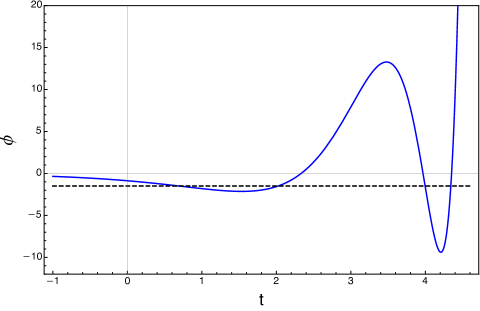
Figure 1: The rolling solution in nonlocal theory with $\xi=0.39$, keeping terms up to $n=30$. The turning point at $\phi=-3/2$ is marked with black dashed line. Similar to the rolling solutions in [19], this also overshoots the turning points and oscillations get larger with time.

To understand the convergence of the series (4.4) describing the rolling, we now attempt to find the behavior of the coefficients $b_{n}$ for $n\to\infty$. A similar analysis for a related solution was done by Fujita and Hata [21]. Our analysis below is not rigorous, but the result is supported by numerical work. The upshot is that for any time $t$ the series solution above converges whenever $\xi^{2}>0$. For $\xi=0$, the series solution converges only until the field reaches the turning point. This will be studied in the next subsection.

By the recursion (4.5) it is clear that the coefficients $b_{n}$ are given by sums of the terms of the form $C_{i}e^{-A_{i}\xi^{2}}$, with $A_{i}$ and $C_{i}$ are some $\xi^{2}$-independent constants. The constants $A_{i}$ are all positive; this follows because the exponent in (4.4) contains the factor $n^{2}-np+p^{2}$, which is positive in the range $1\leq p\leq n-1$. We now assume that $b_{n}$ is dominated by a single term of the form $C_{i}e^{-A_{i}\xi^{2}}$, the one with the lowest value of $A_{i}$. Unless the $C_{i}$ vary wildly, this is the least suppressed term for any nonzero value of $\xi^{2}$. Looking at the recursion (4.5), the sum is modulated by the exponential factor, which is largest at the minimum of $n^{2}-np+p^{2}$. This minimum, with value $3n^{2}/4$, occurs for $p=n/2$ (this is the exact value for the integer $p$ for even $n$, and the approximate value for odd $n$). If this term in the sum dominates, we have the approximate relation valid for very large $n$:

$$b_{n}\simeq\frac{1}{n^{2}}\Bigl{(}b_{\tfrac{n}{2}}\Bigr{)}^{2}\,e^{-\tfrac{3}{2}n^{2}\xi^{2}}\,.$$ (4.7)

Additionally, as stated above, we assume that for large $n$:

$$b_{n}\,\simeq\,C(n)e^{-\alpha(n)\xi^{2}}\,,$$ (4.8)

with constants $C(n)$ and $\alpha(n)>0$ to be determined. Inserting this ansatz into (4.7) we find the conditions:

$$\begin{split}\alpha(n)=2\alpha\left(\tfrac{n}{2}\right)+\tfrac{3}{2}n^{2}\quad\text{and}\quad C(n)=\tfrac{1}{n^{2}}C^{2}\left(\tfrac{n}{2}\right).\end{split}$$ (4.9)

By inspection, these are satisfied by

$$\alpha(n)=3n^{2}\quad\text{and }\quad C(n)=16n^{2}e^{-\beta n},$$ (4.10)

where $\beta\in\mathbb{R}$ is an undetermined constant. From this, $b_{n}$ at large $n$ is given by

$$b_{n}\,\simeq\,(-1)^{n}16n^{2}e^{-\beta n}\,e^{-3n^{2}\xi^{2}},$$ (4.11)

where have also included the correct sign for the coefficient for $b_{n}$. We have determined $\beta\simeq 2$ by fitting–for large $n$–the above expression to numerically calculated coefficients. A couple of fits are shown in figure 2. In fact, the exact value of $\beta$ as well as the prefactor $16n^{2}$ do not affect the following discussion of convergence.

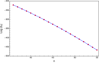
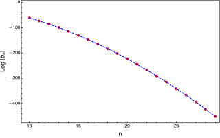
Figure 2: The dots are $\log|b_{n}|$ for $36\leq n\leq 55$ for $\xi=0.2$ (left) and $10\leq n\leq 29$ for $\xi=0.4$ (right), obtained numerically from (4.4). The curves give $\log|b_{n}|$ from the asymptotic result (4.11), with $\beta=2.08$ (left) and $\beta=1.99$ (right). The match of the logarithms is solid, giving evidence for (4.11). We found similar fits for other values of $\xi$ using $\beta\approx 2$.

Consider now the series expansion (4.4) for the rolling tachyon and imagine evaluating the sum for some fixed value $t_{0}$ of the time. To ascertain convergence, we use the ratio test. We consider the absolute value of the ratio of consecutive terms in the expansion, as $n\to\infty$

$$\left|{b_{n+1}e^{(n+1)t_{0}}\over b_{n}e^{nt_{0}}}\right|=\left|{b_{n+1}\over b_{n}}\right|e^{t_{0}}\simeq{(n+1)^{2}\over n^{2}}e^{-\beta}e^{t_{0}}e^{-3(2n+1)\xi^{2}}\,.$$ (4.12)

Due to the last exponent, it is clear that for any value of $t_{0}$ the ratio goes to zero as $n\to\infty$. So the ratio test shows the convergence of the series (4.4) for the nonlocal theory ($\xi^{2}>0$) for any value of $t\in\mathbb{R}$. In practical terms, as the value of time increases we have to include a larger number of terms in the series in order to see the convergence.

4.2 Rolling tachyon perturbatively in $\xi^{2}$

The previous subsection discussed the rolling tachyon nonperturbatively in $\xi^{2}$. The resulting series expansion has coefficients that involve exponentials of $\xi^{2}$, and the series itself is convergent for all values of time. The shortcoming of this solution is that we have not been able to sum the series to arrive a form valid in all times. In this section we work perturbatively in $\xi^{2}$ in order to achieve this. Thus our first step in the analysis would be finding the rolling solution for the local $\xi^{2}=0$ theory. As we will see, an exact analytic solution is possible. Moreover, working perturbatively in $\xi^{2}$ allows to find analytic expressions at each order. This discussion gives further insight into the nature of rolling solutions, and is particularly helpful for small nonlocality.

For the local theory ($\xi^{2}=0$) the rolling solution obtained from the recursion (4.5) is given by:

$$\phi(t)=-e^{t}+\tfrac{1}{3}e^{2t}-\tfrac{1}{12}e^{3t}+\tfrac{1}{54}e^{4t}-\tfrac{5}{1296}e^{5t}+\mathcal{O}(\epsilon^{6t}).$$ (4.13)

It turns out one can sum this series and get a closed form expression:

$$\phi_{0}(t)=-{e^{t}\over(1+\tfrac{1}{6}e^{t})^{2}}\,.$$ (4.14)

This solves the equation of motion (4.3) when $\xi^{2}=0$, with $\phi_{0}\to-e^{t}$ as $t\to-\infty$. The solution shows the scalar rolling down reaching the turning point $\phi=-3/2$ at $e^{t}=6$ and then going back to $\phi=0$ at $t=+\infty$. This result also shows that the series (4.13), arising from expansion of (4.14), converges only for $e^{t}<6$. Observe that the radius of convergence for the series (4.13) turns out to be the time where the tachyon reaches the turning point. The general solution (4.14) is valid for all times and for $e^{t}>6$, so it can be expanded in powers of $e^{-t}$. In fact, for large $t$ we have $\phi\simeq-36e^{-t}$.

Note that we have already argued that the nonlocal version (4.4) of the series solution (4.13) converges for all times, due to the exponential damping associated with $\xi^{2}$. But additionally, it is also clear from the structure of the $b_{n}$ coefficients that

$$|b_{n}(\xi^{2}=0)|\ >\ |b_{n}(\xi^{2}\neq 0)|.$$ (4.15)

It follows that we can conclude rigorously that the series (4.4) converges for $e^{t}<6$ for any $\xi^{2}\neq 0$.

The exact solvability of the local limit of the cubic potential was noticed long ago in the context of lump solutions [25]. With $\xi^{2}=0$, the equation of motion (4.3) can be solved by energy conservation. Since the total energy is zero when the tachyon is at the unstable critical point, and it does not change in time, we have that

$$0={1\over 2}\left({d\phi\over dt}\right)^{2}+{V}(\phi)\implies{d\phi\over dt}=-\sqrt{-2V(\phi)}\,,$$ (4.16)

where the sign is chosen so that the field rolls towards more negative values towards to the stable vacua $\phi=1$. This can be easily integrated, which gives

$$dt=-{d\phi\over\phi\sqrt{1+\tfrac{2}{3}\phi}}\quad\to\quad t-t_{0}=2\tanh^{-1}\sqrt{1+\tfrac{2}{3}\phi\,}\,.$$ (4.17)

Solving for $\phi$ in terms of $t$ one quickly gets

$$\phi(t)=\,-\frac{6e^{t-t_{0}}}{\bigl{(}1+e^{t-t_{0}}\bigr{)}^{2}}\,.$$ (4.18)

The condition $\phi\to-e^{t}$ as $t\to-\infty$ fixes $e^{-t_{0}}={1\over 6}$, and then the solution above coincides with (4.14).

To analyze the nonlocal theory perturbatively in $\xi^{2}$ we begin by expanding the equation of motion (4.3) in powers of $\xi^{2}$:

$$\begin{split}(\partial_{t}^{2}-1)\phi=&\ \phi^{2}-\xi^{2}\left[2(\partial_{t}\phi)^{2}+4\phi(\partial_{t}^{2}\phi)\right]\\ &\ \ \ \,+\xi^{4}\left[4\phi(\partial_{t}^{4}\phi)+6(\partial_{t}\phi)^{2}+8(\partial_{t}\phi)(\partial_{t}^{3}\phi)\right]+\mathcal{O}(\xi^{6}).\end{split}$$ (4.19)

Let the rolling solution $\phi$ for this equation take the form:

$$\phi=\phi_{0}+\xi^{2}\phi_{2}+\xi^{4}\phi_{4}+\mathcal{O}(\xi^{6})\,,$$ (4.20)

with $\phi_{0},\phi_{2},$ and $\phi_{4}$ functions of time to be determined. Inserting this series to the expanded equation of motion above, the first three equations that follow are

$$\begin{split}\mathcal{O}(\xi^{0}):\quad(\partial_{t}^{2}-1)\phi_{0}&=\phi_{0}^{2},\\ \mathcal{O}(\xi^{2}):\quad(\partial_{t}^{2}-1)\phi_{2}&=2\phi_{0}\phi_{2}-2(\partial_{t}\phi_{0})^{2}-4\phi_{0}(\partial_{t}^{2}\phi_{0}),\\ \mathcal{O}(\xi^{4}):\quad(\partial_{t}^{2}-1)\phi_{4}&=2\phi_{0}\phi_{4}+\phi_{2}^{2}-4(\partial_{t}\phi_{0})(\partial_{t}\phi_{2})-4\phi_{0}(\partial_{t}^{2}\phi_{2})-4\phi_{2}(\partial_{t}^{2}\phi_{0})\\ &\hskip 71.13188pt+4\phi_{0}(\partial_{t}^{4}\phi_{0})+6(\partial_{t}\phi_{0})^{2}+8(\partial_{t}\phi_{0})(\partial_{t}^{3}\phi_{0})\,.\end{split}$$ (4.21)

The first one is the equation of motion for the local theory whose rolling solution is already given in (4.14). We have second-order, non-homogeneous linear ordinary differential equations (ODE) at each order and these can be solved recursively. Since we know $\phi_{0}$, we now solve for $\phi_{2}$, and with $\phi_{0}$ and $\phi_{2}$ we can solve for $\phi_{4}$, and so on.

Let us solve for $\phi_{2}$. Inserting the exact solution $\phi_{0}$ in (4.14) and solving the resulting ODE with Mathematica’s DSolve, we obtain the solution:

$$\phi_{2}(t)=\frac{432e^{2t}\left(e^{t}-6\right)}{\left(6+e^{t}\right)^{4}}.$$ (4.22)

The solution from DSolve has two constants of integration. To fix them we imposed two conditions: (i) $\phi_{2}\to 0$ as $t\to-\infty$, and (ii) $\phi_{2}$, expanded in powers of $e^{t}$ must contain no $e^{t}$ term. These are imposed because we want to start the rolling at $\phi=0$, and the $-e^{t}$ term that drives the rolling is already provided by $\phi_{0}$ in (4.14). Carrying the same procedure for the next order we find

$$\phi(t)=-{36e^{t}\over(6+e^{t})^{2}}+\frac{432e^{2t}\left(e^{t}-6\right)}{\left(6+e^{t}\right)^{4}}\xi^{2}-\frac{864e^{2t}\left(2e^{3t}-129e^{2t}+576e^{t}-324\right)}{\left(6+e^{t}\right)^{6}}\xi^{4}+\mathcal{O}(\xi^{6}).$$ (4.23)

This procedure can be repeated recursively to arbitrary order to obtain the exact rolling solutions in the $\xi^{2}$-truncated theories. For higher orders we observed that it was easier to solve the required ODE by guessing an ansatz based on the pattern in (4.23), rather than using DSolve. In figure 3 to the left, we show the rolling solution (4.23), extended to ${\cal O}(\xi^{8})$ and then truncated at various orders; to the right, we show the ${\cal O}(\xi^{8})$ solution together with the series solution in $e^{nt}$. It seems clear that as one includes higher orders in $\xi^{2}$, the behavior of the rolling solution approaches that of the nonlocal theory. Indeed, we have checked that the solution (4.23) matches with the rolling solution (4.4) perturbatively up to the order $\mathcal{O}(\xi^{8},e^{14t})$.

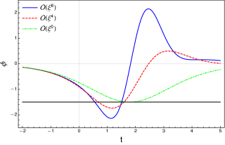
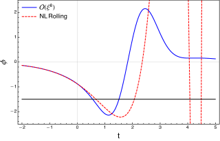
Figure 3: In both plots $\xi=0.4$. Left: The rolling solution (4.23) to orders $\mathcal{O}(\xi^{4}i)$ and $\mathcal{O}(\xi^{8})$, shown together with the rolling in the local theory. Right: The rolling solution to order $\mathcal{O}(\xi^{8})$ compared to the nonlocal theory rolling based on (4.4), including $b_{n}$ up to $n\leq 14$. The turning point at $\phi=-3/2$ is marked with straight black lines.

4.3 Rolling solution after field redefinition

Now that we have control over the rolling solution of the nonlocal theory, we can test our work in redefining the theory into a local one for the purely time-dependent fields. The expectation is that the wild oscillations of the nonlocal theory tachyon should turn into smooth rolling in the potential $V$ for the new redefined field. We can test this concretely, since we have already determined the field redefinition. This is a consistency check for the field redefinition, and for the claimed equivalence of the nonlocal theory to the local $\xi^{2}$-dependent theory.

To deal with the field redefinition, we have to introduce a bit of notation that we did not use in the previous section. We will still call $\phi$ the original field of the nonlocal theory, but we will call $\phi^{\prime}$ the field of the redefined theory. Our work before was based on replacements of the form

$$\phi\ \to\phi+\delta\phi(\phi,\partial\phi)\,,$$ (4.24)

implemented directly on the Lagrangian as in $L[\phi]\to L[\phi+\delta\phi]$, a replacement that yields an equivalent Lagrangian. But now the field in the final Lagrangian must be called $\phi^{\prime}$, this actually means that we are setting

$$\phi=\phi^{\prime}+\delta\phi(\phi^{\prime},\partial\phi^{\prime})\,,$$ (4.25)

so in order to demonstrate the taming of the wild $\phi$-field oscillations, we must calculate $\phi^{\prime}$ in terms of $\phi$ and its derivatives, and then use the rolling solution for $\phi$ in (4.23) to calculate the rolling solution $\phi^{\prime}$ in the redefined theory. Both the field redefinition and this rolling solution are perturbative in $\xi^{2}$.

To calculate $\phi^{\prime}$ we have to perturbatively invert the field redefinition (3.53) we found before. In the $\phi,\phi^{\prime}$ notation we are now using, this reads to $\mathcal{O}(\xi^{4})$,

$$\begin{split}\phi&=\phi^{\prime}-\xi^{2}{\phi^{\prime}}^{2}+\xi^{4}\Bigl{[}(1+c_{3,0})\tfrac{3}{2}{\phi^{\prime}}^{2}+\left(\tfrac{13}{3}+c_{3,0}\right){\phi^{\prime}}^{3}\\ &\hskip 142.26378pt+(1-3c_{3,0})(\partial_{t}\phi^{\prime})^{2}+2\phi^{\prime}(\partial_{t}^{2}\phi^{\prime})\bigg{]}+\mathcal{O}(\xi^{6}),\end{split}$$ (4.26)

The inversion can be done perturbative by writing the ansatz

$$\phi^{\prime}=\phi_{0}^{\prime}+\xi^{2}\phi_{2}^{\prime}+\xi^{4}\phi_{4}^{\prime}+\mathcal{O}(\xi^{6}),$$ (4.27)

and inserting this expression into (4.26) to solve recursively for $\phi_{0}^{\prime},\phi_{2}^{\prime},\phi_{4}^{\prime},\ldots$. The end result can be found after some algebra and it is

$$\begin{split}\phi^{\prime}&=\phi+\xi^{2}\phi^{2}+\xi^{4}\Bigl{[}\tfrac{3}{2}(-c_{3,0}-1)\phi^{2}+\left(-c_{3,0}-\tfrac{7}{3}\right)\phi^{3}\\ &\hskip 113.81102pt-\left(1-3c_{3,0}\right)(\partial_{t}\phi)^{2}-2\phi(\partial_{t}^{2}\phi)\Bigr{]}+\mathcal{O}(\xi^{6}).\end{split}$$ (4.28)

Setting $\phi$ equal to the rolling solution (4.23), we can evaluate the right-hand side of the equation above and find that

$$\begin{split}\phi^{\prime}(t)=&-{36e^{t}\over(6+e^{t})^{2}}+\frac{432e^{2t}\left(e^{t}-3\right)}{\left(6+e^{t}\right)^{4}}\xi^{2}\\ &-\frac{216e^{2t}}{\left(6+e^{t}\right)^{6}}\left(8e^{3t}+\left(-9c_{3,0}-345\right)e^{2t}+36\left(19+3c_{3,0}\right)e^{t}+324\left(-c_{3,0}-1\right)\right)\,\xi^{4}+\mathcal{O}(\xi^{6}).\end{split}$$ (4.29)

We have carried this procedure up to $\mathcal{O}(\xi^{8})$ and checked that the resulting $\phi^{\prime}$ satisfies the equation for conventional rolling in the potential $\tilde{V}(\phi^{\prime};\xi^{2})$ in (3.52), truncated to $\mathcal{O}(\xi^{8})$.

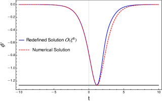
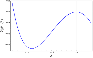
Figure 4: Plots calculated to ${\cal O}(\xi^{8})$ and setting $\xi=0.3$. Left: The redefined solution $\phi^{\prime}(t)$ compared to the rolling solution in $\tilde{V}(\phi^{\prime};\xi^{2})$. The black line denotes the value $\phi^{\prime}\simeq-1.27$ of the turning point in $\tilde{V}(\phi^{\prime};\xi^{2})$. Neither solution overshoots this turning point. Right: The potential $\tilde{V}(\phi^{\prime};\xi^{2})$.

Assume the constants $c_{i,j}$ take the values in (3.54), fixing the ambiguity of the potential. Working to ${\cal O}(\xi^{8})$ and taking $\xi=0.3$, figure 4, left, shows the numerical rolling solution for the potential $\tilde{V}(\phi^{\prime},\xi^{2})$ as well as redefined solution $\phi^{\prime}(t)$ above. As expected, but nonetheless still quite striking, the overshooting of the turning point has disappeared for the field variable $\phi^{\prime}$. The redefined and numerical solutions match before the turning point, but they differ slightly afterwards. We have observed that including more orders in $\xi$ improves the matching between these solutions. The potential $\tilde{V}(\phi;\xi^{2})$ itself is shown to the right. The comparison of the redefined rolling solution (4.29) with the rolling solution (4.4) of the original nonlocal theory for $\xi=0.35$ is shown in figure 5. We checked that similar behavior holds for potentials related by quasi-symmetries. The lack of late-time oscillations in the redefined solution is an automatic feature of the expansion. One must go to much higher orders in $\xi^{2}$ to truly test the disappearance of oscillations.

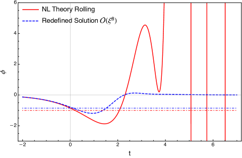
Figure 5: Comparison between the solutions (4.4) (solid red) and (4.29) (dashed blue) when $\xi=0.35$. The color-coded dot-dash horizontal lines mark the stable vacua of their respective potentials. Notice their first pass through the minimum occur roughly at the same time.

5 Noncovariant redefinitions of the general nonlocal theory

In this section, we extend the previous analysis of the solely time-dependent theory to the case of the completely general spacetime-dependent Lorentz-covariant Lagrangian:

$$L=\tfrac{1}{2}\,\phi\partial^{2}\phi+\tfrac{1}{2}\,\phi^{2}+\tfrac{1}{3}\,\big{(}e^{\xi^{2}\partial^{2}}\phi\big{)}^{3}.$$ (5.1)

We ask if it is possible to remove higher-order derivatives perturbatively in $\xi^{2}$ using a field redefinition while keeping manifest Lorentz covariance. Up to and including ${\cal O}(\xi^{6})$ terms we see that this is possible. At ${\cal O}(\xi^{8})$, however, we encounter an obstruction: we cannot eliminate certain higher-derivative terms covariantly. So instead, we settle for removing just higher-order time derivatives, since this suffices for setting up a well-posed initial value problem. We show that this can be achieved at ${\cal O}(\xi^{8})$, and then provide a general argument that this can be achieved for all orders.

Defining an obstruction as a higher-derivative term that cannot be removed from the theory covariantly, we will adapt the following strategy for field redefinitions. At any fixed order in $\xi^{2}$, after dealing with the lower-order terms we must

1. Remove all higher-order derivative terms that can be dealt with covariantly

2. Remove terms of the form $\phi^{n}(\partial\phi)^{2}$ for $n\geq 1$ in order to have a standard kinetic term.

3. Remove higher-order time derivatives from obstruction terms by breaking the manifest Lorentz covariance.

4. Repeat the steps above if additional higher-derivative or $\phi^{n}(\partial\phi)^{2}$ terms are introduced by the previous step.

Since the field redefinition $\delta\phi$ multiplies $\partial^{2}\phi$ (or $\partial_{t}^{2}\phi$), we need to apply successive redefinitions to decrease the total derivative order in steps of two. The end result would be a collection of terms in which there are only first order time derivatives, coming in arbitrary numbers. Note that not all terms with first-order derivatives can be removed since equation (3.30), which allowed us to do this in the time-dependent case, does not have a generalization to the general spacetime-dependent case. An immediate consequence is that the potential obtained in this section will be different from the one obtained in the purely time-dependent theory.

Alternatively, it is possible to write the Lagrangian (5.1) in the light-cone frame and give the theory an initial value formulation by eliminating all derivatives with respect to light-cone time $\tau\equiv x^{+}\equiv(x^{0}+x^{1})/2$, except the one that appears in the kinetic term. We will see this requires the familiar light-cone nonlocalities—inverse $x^{-}\equiv(x^{0}-x^{1})/2$ derivatives.

In subsection 5.1 we explicitly implement the algorithm above to ${\cal O}(\xi^{8})$ to display the first obstruction to a Lorentz covariant field redefinition, and to show how one implements the elimination of higher-order time derivatives in this case. Then, in subsection 5.2, we provide a general algorithm to carry out the procedure to all orders. A brief description of Hamiltonian formulation of the theory is given in subsection 5.3. The light-cone formulation of the theory is discussed in subsection 5.4.

5.1 Redefinitions up to ${\cal O}(\xi^{8})$

We begin by expanding the Lagrangian (5.1) in powers of $\xi^{2}$. To $\mathcal{O}(\xi^{8})$, we find

$$L=\tfrac{1}{2}\,\phi\partial^{2}\phi +\tfrac{1}{2}\,\phi^{2}+\tfrac{1}{3}\,\phi^{3}+\xi^{2}\,\phi^{2}\partial^{2}\phi+\xi^{4}\left(\tfrac{1}{2}\,\phi^{2}\partial^{4}\phi+\phi(\partial^{2}\phi)^{2}\right)$$ (5.2)

$$+\tfrac{1}{3}\,\xi^{6}\left(\tfrac{1}{2}\,\phi^{2}\partial^{6}\phi+3\phi\partial^{2}\phi\partial^{4}\phi+(\partial^{2}\phi)^{3}\right)$$

$$+\tfrac{1}{3}\xi^{8}\left(\tfrac{1}{8}\,\phi^{2}\partial^{8}\phi+\phi\partial^{2}\phi\partial^{6}\phi+\tfrac{3}{4}\,\phi(\partial^{4}\phi)^{2}+\tfrac{3}{2}\,(\partial^{2}\phi)^{2}\partial^{4}\phi\right)+\mathcal{O}(\xi^{10}).$$

Using the field redefinition

$$\phi\longrightarrow\phi+\xi^{2}\delta_{2}\phi+\xi^{4}\delta_{4}\phi+\xi^{6}\delta_{6}\phi+\xi^{8}\delta_{8}\phi+\mathcal{O}(\xi^{10})\,,$$ (5.3)

the field-redefined Lagrangian $(L\to\tilde{L})$ takes the following form:

$$\tilde{L}\equiv\sum_{n=0}^{\infty}\xi^{2n}\tilde{L}_{2n}\,,$$ (5.4)

where

$$\tilde{L}_{0}=\ \tfrac{1}{2}\,\phi\partial^{2}\phi+\tfrac{1}{2}\,\phi^{2}+\tfrac{1}{3}\,\phi^{3}\,,$$ (5.5)

$$\tilde{L}_{2}=\phi^{2}\partial^{2}\phi+\delta_{2}\phi\partial^{2}\phi+(\phi^{2}+\phi)\delta_{2}\phi\,,$$ (5.6)

$$\tilde{L}_{4}=\tfrac{1}{2}\,\phi^{2}\partial^{4}\phi +\phi(\partial^{2}\phi)^{2}+\delta_{4}\phi\,\partial^{2}\phi+(\phi^{2}+\phi)\,\delta_{4}\phi$$ (5.7)

$$+2\phi\delta_{2}\phi\partial^{2}\phi+\phi^{2}\partial^{2}\delta_{2}\phi+\tfrac{1}{2}\delta_{2}\phi\partial^{2}\delta_{2}\phi+\delta_{2}\phi(\tfrac{1}{2}+\phi)\delta_{2}\phi\,,$$

$$\tilde{L}_{6}=\tfrac{1}{6}\phi^{2}\partial^{6}\phi +\phi(\partial^{2}\phi)(\partial^{4}\phi)+\tfrac{1}{3}(\partial^{2}\phi)^{3}+\delta_{6}\phi\partial^{2}\phi+(\phi^{2}+\phi)\partial\phi_{6}+\delta_{4}\phi\partial^{2}\delta_{2}\phi$$

$$+(2\phi+1)\delta_{2}\phi\delta_{4}\phi+\tfrac{1}{3}(\delta_{2}\phi)^{3}+\phi^{2}\partial^{2}\delta_{4}\phi+2\phi\delta_{4}\phi\partial^{2}\phi+(\delta_{2}\phi)^{2}\partial^{2}\phi$$

$$+2\phi\delta_{2}\phi\partial^{2}\delta_{2}\phi+\phi\delta_{2}\phi\partial^{4}\phi+\tfrac{1}{2}\phi^{2}\partial^{4}\delta_{2}\phi+\delta_{2}\phi(\partial^{2}\phi)^{2}+2\phi(\partial^{2}\phi)(\partial^{2}\delta_{2}\phi)\,,$$

$$\tilde{L}_{8}=\tfrac{1}{24}\phi^{2}\partial^{8}\phi +\tfrac{1}{3}\phi(\partial^{2}\phi)(\partial^{6}\phi)+\tfrac{1}{4}\phi(\partial^{4}\phi)^{2}+\tfrac{1}{2}(\partial^{2}\phi)^{2}(\partial^{4}\phi)+\tfrac{1}{6}\phi^{2}\partial^{6}\delta_{2}\phi+\tfrac{1}{3}\phi\delta_{2}\phi\partial^{6}\phi$$ (5.8)

$$+\phi(\partial^{2}\phi)\partial^{4}\delta_{2}\phi+\phi(\partial^{2}\delta_{2}\phi)\partial^{4}\phi+\delta_{2}\phi(\partial^{2}\phi)(\partial^{4}\phi)+(\partial^{2}\phi)^{2}\partial^{2}\delta_{2}\phi+\phi\delta_{2}\phi\partial^{4}\delta_{2}\phi$$

$$+\tfrac{1}{2}(\delta_{2}\phi)^{2}\partial^{4}\phi+\phi(\partial^{2}\delta_{2}\phi)^{2}+2\delta_{2}\phi(\partial^{2}\delta_{2}\phi)\partial^{2}\phi+(\delta_{2}\phi)^{2}\partial^{2}\delta_{2}\phi+2\phi\delta_{4}\phi\partial^{2}\delta_{2}\phi$$

$$+2\phi\delta_{2}\phi\partial^{2}\delta_{4}\phi+2\delta_{2}\phi\delta_{4}\phi\partial^{2}\phi+(\delta_{2}\phi)^{2}\delta_{4}\phi+\delta_{2}\phi\partial^{2}\delta_{6}\phi+(1+2\phi)\delta_{2}\phi\delta_{6}\phi$$

$$+\tfrac{1}{2}\phi^{2}\partial^{4}\delta_{4}\phi+\phi\delta_{4}\phi\partial^{4}\phi+2\phi(\partial^{2}\phi)\partial^{2}\delta_{4}\phi+\delta_{4}\phi(\partial^{2}\phi)^{2}+\tfrac{1}{2}(\delta_{4}\phi)^{2}+\tfrac{1}{2}\delta_{4}\phi\partial^{2}\delta_{4}\phi$$

$$+\phi(\delta_{4}\phi)^{2}+\phi^{2}\partial^{2}\delta_{6}\phi+2\phi\delta_{6}\phi\partial^{2}\phi+\delta_{8}\phi\partial^{2}\phi+(\phi^{2}+\phi)\delta_{8}\phi\,.$$

Starting at ${\cal O}(\xi^{2})$, choosing $\delta_{2}\phi=-\phi^{2}$ eliminates the term $\phi^{2}\partial^{2}\phi$ and leaves us with no derivatives:

$$\tilde{L}_{2}=-\phi^{3}-\phi^{4}\,.$$ (5.9)

Using the chosen $\delta_{2}\phi$ and integrating-by-parts, we see $\tilde{L}_{4}$ takes the form

$$\tilde{L}_{4}\simeq\partial^{2}\phi\bigg{[}\delta_{4}\phi+\tfrac{1}{2}\,\partial^{2}\phi^{2}+\phi\partial^{2}\phi-2\phi^{3}\bigg{]}+(\phi^{2}+\phi)\,\delta_{4}\phi+\tfrac{1}{2}\phi^{4}+\phi^{5}+2\phi^{2}(\partial\phi)^{2}.$$ (5.10)

We now choose

$$\delta_{4}\phi=\delta_{4}\phi^{\prime}-\tfrac{1}{2}\,\partial^{2}\phi^{2}-\phi\partial^{2}\phi+2\phi^{3},$$ (5.11)

including a $\delta_{4}\phi^{\prime}$ for further redefinitions. We then find

$$\begin{split}\tilde{L}_{4}&\simeq\partial^{2}\phi\,\delta_{4}\phi^{\prime}+(\phi^{2}+\phi)\,\bigg{[}\delta_{4}\phi^{\prime}-\tfrac{1}{2}\,\partial^{2}\phi^{2}-\phi\partial^{2}\phi+2\phi^{3}\bigg{]}+\tfrac{1}{2}\phi^{4}+\phi^{5}+2\phi^{2}(\partial\phi)^{2}\\ &\simeq\partial^{2}\phi\bigg{[}\delta_{4}\phi^{\prime}-\tfrac{1}{2}\phi^{2}-(\phi^{2}+\phi)\phi\bigg{]}+(\phi^{2}+\phi)\delta_{4}\phi^{\prime}+\tfrac{5}{2}\phi^{4}+3\phi^{5}+4\phi^{2}(\partial\phi)^{2},\end{split}$$ (5.12)

after arranging terms and integrating by parts. Further, we can pick

$$\delta_{4}\phi^{\prime}=\tfrac{1}{2}\phi^{2}+(\phi^{2}+\phi)\phi=\phi^{3}+\tfrac{3}{2}\phi^{2},$$ (5.13)

and this eliminates the remaining higher-order derivative terms and yields

$$\begin{split}\tilde{L}_{4}\simeq(\phi^{2}+\phi)\big{(}\phi^{3}+\tfrac{3}{2}\phi^{2}\big{)}+\tfrac{5}{2}\phi^{4}+3\phi^{5}+4\phi^{2}(\partial\phi)^{2}=\tfrac{3}{2}\phi^{3}+5\phi^{4}+4\phi^{5}+4\phi^{2}(\partial\phi)^{2}.\end{split}$$ (5.14)

We can also eliminate the term $4\phi^{2}(\partial\phi)^{2}$ covariantly. For generality, we will show how to eliminate the generic term $\phi^{n}(\partial\phi)^{2}$, where $n$ is a positive integer. Integrating-by-parts, we see such term can be written as

$$\begin{split}\phi^{n}(\partial\phi)^{2}&\simeq-\phi\partial_{\mu}(\phi^{n}\partial^{\mu}\phi)=-n\phi^{n}(\partial\phi)^{2}-\phi^{n+1}\partial^{2}\phi\\ &\implies\phi^{n}(\partial\phi)^{2}\simeq-\tfrac{1}{n+1}\phi^{n+1}\partial^{2}\phi.\end{split}$$ (5.15)

Notice the similarity between this argument and that given in (3.30). The above holds only when we have two derivatives, otherwise the contractions of Lorentz indices do not work out. Suppose now that the Lagrangian at order $\xi^{2k}$ contains a term of the form $\beta\phi^{n}(\partial\phi)^{2}$, with $\beta$ a constant. This term can be eliminated with a field redefinition $\phi\to\phi+\xi^{2k}\delta_{2k}\widetilde{\phi}$, as follows:

$$\begin{split}T_{2k}&\equiv\delta_{2k}\widetilde{\phi}(\partial^{2}\phi+\phi+\phi^{2})+\beta\phi^{n}(\partial\phi)^{2}\\ &\simeq\partial^{2}\phi(\delta_{2k}\widetilde{\phi}-\tfrac{\beta}{n+1}\phi^{n+1})+\delta_{2k}\widetilde{\phi}(\phi+\phi^{2}).\end{split}$$ (5.16)

We then fix the redefinition and find:

$$\delta_{2k}\widetilde{\phi}=\tfrac{\beta}{n+1}\phi^{n+1}\quad\to\quad T_{2k}=\tfrac{\beta}{n+1}\phi^{n+2}+\tfrac{\beta}{n+1}\phi^{n+3}.$$ (5.17)

In particular, this shows the term $4\phi^{2}(\partial\phi)^{2}$ in (5.14) can be redefined to

$$4\phi^{2}(\partial\phi)^{2}\to\tfrac{4}{3}\phi^{4}+\tfrac{4}{3}\phi^{5}\ \ \hbox{with}\ \ \delta_{4}\widetilde{\phi}=\tfrac{4}{3}\phi^{3}\,.$$ (5.18)

Combining this with the rest at this order we see that

$$\tilde{L}_{4}\simeq\tfrac{3}{2}\phi^{3}+\tfrac{19}{3}\phi^{4}+\tfrac{16}{3}\phi^{5}.$$ (5.19)

Including $\delta_{4}\widetilde{\phi}$ in $\delta_{4}\phi$, the total field redefinition at order $\mathcal{O}(\xi^{4})$ to reach this form is

$$\delta_{4}\phi=-\tfrac{1}{2}\,\partial^{2}\phi^{2}-\phi\partial^{2}\phi+\tfrac{13}{3}\phi^{3}+\tfrac{3}{2}\phi^{2}.$$ (5.20)

As one can see, all derivatives have been eliminated to this order as well. The results so far are the same as those for the purely-time-dependent case (3.32) after replacing $\partial_{t}\to\partial$ and taking a minus sign into account, as we essentially implemented a similar procedure.

Repeating the analysis to ${\cal O}(\xi^{6})$ we find

$$\tilde{L}_{6} \simeq-\big{(}\tfrac{3}{2}\phi^{3}+\tfrac{178}{9}\phi^{4}+\tfrac{472}{9}\phi^{5}+\tfrac{112}{3}\phi^{6}\big{)}-\tfrac{8}{3}(\partial\phi)^{4},$$ (5.21)

after fixing the field redefinition as follows

$$\delta_{6}\phi =-\tfrac{1}{6}\partial^{4}\phi^{2}-\phi\partial^{4}\phi-\tfrac{1}{3}(\partial^{2}\phi)^{2}+18\phi^{2}\partial^{2}\phi$$ (5.22)

$$\quad+\tfrac{8}{3}\phi\partial^{2}\phi+\tfrac{70}{3}\phi(\partial\phi)^{2}+\tfrac{7}{3}(\partial\phi)^{2}-\tfrac{85}{3}\phi^{4}-\tfrac{151}{9}\phi^{3}-\tfrac{3}{2}\phi^{2}.$$

The $(\partial\phi)^{4}$ term in $\tilde{L}_{6}$ cannot be written as $(\partial\phi)^{4}=\partial^{2}\phi[\cdots]$ so it cannot get eliminated covariantly. But as explained before, this is not a higher derivative term, and it is no obstacle for an initial value formulation. The obstacle appears at next order, as we now show.

Repeating now the analysis to ${\cal O}(\xi^{8})$, successive field redefinitions remove all higher-order derivatives except for the term of the form $(\partial\phi)^{2}\partial^{2}(\partial\phi)^{2}$, which is an obstruction:

$$\tilde{L}_{8} \simeq\tfrac{9}{8}\phi^{3}+\tfrac{223}{6}\phi^{4}+\tfrac{483}{2}\phi^{5}+485\phi^{6}+\tfrac{2695}{9}\phi^{7}$$ (5.23)

$$\quad+\left(\tfrac{52}{3}+96\phi\right)(\partial\phi)^{4}-\tfrac{4}{3}\,(\partial\phi)^{2}\partial^{2}(\partial\phi)^{2}\,.$$

We omit the total redefinition to this order since it is rather long and unenlightening. The term $(\partial\phi)^{2}\partial^{2}(\partial\phi)^{2}$ in $\tilde{L}_{8}$ cannot be removed covariantly: no integration by parts allows it to be written in the factorized form $\partial^{2}\phi[\cdots]$ required for covariant elimination. We will therefore break manifest Lorentz covariance and focus on removing only higher-order time derivatives.

Focusing on the obstruction term $(\partial\phi)^{2}\partial^{2}(\partial\phi)^{2}$, we first evaluate the part of the term multiplying $(\partial\phi)^{2}$ by breaking derivatives into temporal and spatial parts:

$$\partial^{2}(\partial\phi)^{2} =(-\partial_{t}^{2}+\boldsymbol{\nabla}^{2})\big{(}-\dot{\phi}^{2}+(\boldsymbol{\nabla}\phi)^{2}\big{)}$$

$$=\partial_{t}^{2}(\dot{\phi}^{2})-\partial_{t}^{2}(\boldsymbol{\nabla}\phi)^{2}-\boldsymbol{\nabla}^{2}(\dot{\phi}^{2})+\boldsymbol{\nabla}^{2}(\boldsymbol{\nabla}\phi)^{2}$$

$$=2\dot{\phi}\phi^{(3)}+2\ddot{\phi}^{2}-2\boldsymbol{\nabla}\phi\cdot\boldsymbol{\nabla}\ddot{\phi}-4(\boldsymbol{\nabla}\dot{\phi})^{2}-2\dot{\phi}\boldsymbol{\nabla}^{2}\dot{\phi}+2\boldsymbol{\nabla}\phi\cdot\boldsymbol{\nabla}(\boldsymbol{\nabla}^{2}\phi)+2(\nabla_{i}\nabla_{j}\phi)^{2}$$

$$=2\big{[}\dot{\phi}\phi^{(3)}+\ddot{\phi}^{2}-\boldsymbol{\nabla}\phi\cdot\boldsymbol{\nabla}\ddot{\phi}-2(\boldsymbol{\nabla}\dot{\phi})^{2}+\partial^{\mu}\phi\partial_{\mu}(\boldsymbol{\nabla}^{2}\phi)+(\nabla_{i}\nabla_{j}\phi)^{2}\big{]}.$$

Here, we use $\phi^{(n)}\equiv\partial_{t}^{n}\phi$. Performing the field redefinition $\phi\to\phi+\xi^{8}\delta_{8}\hat{\phi}$ and letting $\tilde{T}_{8}$ denote the part of $\tilde{L}_{8}$ that contains the field redefinition and the obstruction term, we have

$$\widetilde{T}_{8} =-\ddot{\phi}\,\delta_{8}\hat{\phi}+(\boldsymbol{\nabla}^{2}\phi+\phi^{2}+\phi)\delta_{8}\hat{\phi}$$

$$\qquad-\tfrac{8}{3}\,(\partial\phi)^{2}\Big{(}\dot{\phi}\phi^{(3)}+\ddot{\phi}^{2}-\boldsymbol{\nabla}\phi\cdot\boldsymbol{\nabla}\ddot{\phi}-2(\boldsymbol{\nabla}\dot{\phi})^{2}+\partial^{\mu}\phi\partial_{\mu}(\boldsymbol{\nabla}^{2}\phi)+(\nabla_{i}\nabla_{j}\phi)^{2}\Big{)}$$

$$\simeq\ddot{\phi}\,\Big{(}-\delta_{8}\hat{\phi}-\tfrac{8}{3}\,(\partial\phi)^{2}\ddot{\phi}-\tfrac{8}{3}\,\nabla^{i}\big{(}(\partial\phi)^{2}\nabla_{i}\phi\big{)}+\tfrac{8}{3}\,\partial_{t}\big{(}(\partial\phi)^{2}\,\dot{\phi}\big{)}\Big{)}+(\boldsymbol{\nabla}^{2}\phi+\phi^{2}+\phi)\delta_{8}\hat{\phi}$$

$$\qquad-\tfrac{8}{3}\,(\partial\phi)^{2}\Big{(}-2(\boldsymbol{\nabla}\dot{\phi})^{2}+\partial^{\mu}\phi\,\partial_{\mu}(\boldsymbol{\nabla}^{2}\phi)+(\nabla_{i}\nabla_{j}\phi)^{2}\Big{)}.$$

Now fixing

$$\delta_{8}\hat{\phi}=\delta_{8}\hat{\phi}^{\prime}-\tfrac{8}{3}\,(\partial\phi)^{2}\ddot{\phi}-\tfrac{8}{3}\,\partial^{\mu}\big{(}(\partial\phi)^{2}\partial_{\mu}\phi\big{)},$$ (5.24)

we see that $\tilde{L}_{8}$ becomes, after some calculation,

$$\widetilde{T}_{8} \simeq\ddot{\phi}\,\Big{(}-\delta_{8}\hat{\phi}^{\prime}-\tfrac{8}{3}\,(\partial\phi)^{2}(\boldsymbol{\nabla}^{2}\phi+\phi^{2}+\phi)\Big{)}+(\boldsymbol{\nabla}^{2}\phi+\phi^{2}+\phi)\delta_{8}\hat{\phi}^{\prime}$$

$$\qquad-\tfrac{8}{3}\,(\partial\phi)^{2}\Big{(}(\nabla_{i}\nabla_{j}\phi)^{2}-\partial^{\mu}\phi\,\partial_{\mu}(\phi^{2}+\phi)-2(\boldsymbol{\nabla}\dot{\phi})^{2}\Big{)}.$$

We then take

$$\delta_{8}\hat{\phi}^{\prime}=\delta_{8}\hat{\phi}^{\prime\prime}-\tfrac{8}{3}\,(\partial\phi)^{2}(\boldsymbol{\nabla}^{2}\phi+\phi^{2}+\phi),$$ (5.25)

and after some simplification, we find

$$\widetilde{T}_{8} \simeq(\partial^{2}\phi+\phi^{2}+\phi)\delta_{8}\hat{\phi}^{\prime\prime}+\tfrac{8}{3}(2\phi+1)(\partial\phi)^{4}-\tfrac{8}{3}(\phi^{2}+\phi)^{2}(\partial\phi)^{2}$$ (5.26)

$$\qquad-\tfrac{8}{3}\,(\partial\phi)^{2}\Big{(}(\boldsymbol{\nabla}^{2}\phi)^{2}+(\nabla_{i}\nabla_{j}\phi)^{2}-2(\boldsymbol{\nabla}\dot{\phi})^{2}+2(\phi^{2}+\phi)\boldsymbol{\nabla}^{2}\phi\Big{)}.$$

Finally, we can eliminate the term $-\tfrac{8}{3}(\phi^{2}+\phi)^{2}(\partial\phi)^{2}=-\tfrac{8}{3}(\phi^{2}+2\phi^{3}+\phi^{4})(\partial\phi)^{2}$ by taking

$$\delta_{8}\hat{\phi}^{\prime\prime}=-\tfrac{8}{15}\phi^{5}-\tfrac{4}{3}\phi^{4}+\tfrac{8}{9}\phi^{3}\,.$$ (5.27)

This yields

$$\widetilde{T}_{8} \simeq-\tfrac{8}{9}\phi^{4}-\tfrac{20}{9}\phi^{5}-\tfrac{28}{15}\phi^{6}-\tfrac{8}{16}\phi^{7}+\tfrac{8}{3}(2\phi+1)(\partial\phi)^{4}$$ (5.28)

$$\qquad-\tfrac{8}{3}\,(\partial\phi)^{2}\Big{(}(\boldsymbol{\nabla}^{2}\phi)^{2}+(\nabla_{i}\nabla_{j}\phi)^{2}-2(\boldsymbol{\nabla}\dot{\phi})^{2}+2(\phi^{2}+\phi)\boldsymbol{\nabla}^{2}\phi\Big{)}.$$

Combining $\widetilde{T}_{8}$ with the rest of $\tilde{L}_{8}$, we finally get

$$\tilde{L}_{8} \simeq\tfrac{9}{8}\phi^{3}+\tfrac{653}{18}\phi^{4}+\tfrac{4307}{18}\phi^{5}+\tfrac{7247}{15}\phi^{6}+\tfrac{13451}{45}\phi^{7}+\left(20+\tfrac{304}{3}\phi\right)(\partial\phi)^{4}$$ (5.29)

$$\qquad-\tfrac{8}{3}\,(\partial\phi)^{2}\Big{(}(\boldsymbol{\nabla}^{2}\phi)^{2}+(\nabla_{i}\nabla_{j}\phi)^{2}-2(\boldsymbol{\nabla}\dot{\phi})^{2}+2(\phi^{2}+\phi)\boldsymbol{\nabla}^{2}\phi\Big{)}.$$

We no longer have higher time derivatives, but higher spatial derivatives remain.

Summarizing, the total Lagrangian after field redefinition can be written as:

$$\tilde{L}\simeq-\tilde{K}(\phi,\dot{\phi},\boldsymbol{\nabla}\phi;\xi^{2})-\tilde{V}(\phi;\xi^{2}),$$ (5.30)

where

$$\tilde{K}(\phi,\dot{\phi},\boldsymbol{\nabla}\phi;\xi^{2}) =\tfrac{1}{2}\,(\partial\phi)^{2}+\left(\tfrac{8}{3}\,\xi^{6}-20\xi^{8}\right)(\partial\phi)^{4}-\tfrac{304}{3}\xi^{8}\phi(\partial\phi)^{4}$$ (5.31)

$$\quad\ +\tfrac{8}{3}\,\xi^{8}(\partial\phi)^{2}\Big{(}(\boldsymbol{\nabla}^{2}\phi)^{2}+(\nabla_{i}\nabla_{j}\phi)^{2}-2(\boldsymbol{\nabla}\dot{\phi})^{2}+2(\phi^{2}+\phi)\boldsymbol{\nabla}^{2}\phi\Big{)}+\,{\cal O}(\xi^{10}),$$

and

$$\tilde{V}(\phi;\xi^{2})=-\tfrac{1}{2}\,\phi^{2} -\tfrac{1}{3}\,e^{-3\xi^{2}}\,\phi^{3}+\left[\xi^{2}-\tfrac{19}{3}\xi^{4}+\tfrac{178}{9}\xi^{6}-\tfrac{653}{18}\xi^{8}+\cdots\right]\,\phi^{4}$$ (5.32)

$$+\left[-\tfrac{16}{3}\xi^{4}+\tfrac{472}{9}\xi^{6}-\tfrac{4307}{18}\xi^{8}+\cdots\right]\,\phi^{5}$$

$$+\left[\tfrac{112}{3}\xi^{6}-\tfrac{7247}{15}\xi^{8}+\cdots\right]\,\phi^{6}+\left[-\tfrac{13451}{45}\xi^{8}+\cdots\right]\,\phi^{7}+\mathcal{O}(\phi^{8}).$$

In the potential we have summed the series in front of the cubic term:

$$e^{-3\xi^{2}}=1-3\xi^{2}+\tfrac{9}{2}\xi^{4}-\tfrac{9}{2}\xi^{6}+\tfrac{27}{8}\xi^{8}+\cdots$$ (5.33)

It is possible to prove this result as follows. First note that since the field redefinition $\delta\phi$ is at least quadratic in $\phi$, cubic terms in the Lagrangian can be generated only by variations linear in $\delta\phi$ of quadratic terms in the Lagrangian. In other words, cubic terms are generated from $\delta\phi(\partial^{2}\phi+\phi+\phi^{2})$, and only when trying to remove higher derivatives from the original cubic interactions of the nonlocal theory—quartic and higher order terms in $\phi$ induced by the redefinition process cannot generate cubic terms. As a consequence, the effective rule for the generation of cubic terms from the field redefinition is the replacement $\partial^{2}\phi\to-\phi$ on cubic terms. This means that $(e^{\xi^{2}\partial^{2}}\phi)^{3}\to(e^{-\xi^{2}}\phi)^{3}$. This makes clear the on-shell three-point amplitude in the redefined theory agrees to all orders in $\xi^{2}$ with the one derived from the original theory. We have also checked that the on-shell four-point amplitude with the redefined Lagrangian agrees with the one computed from the original Lagrangian up to and including $\mathcal{O}(\xi^{4})$.

As a check of this potential, we have also verified that its value at the critical point, computed to ${\cal O}(\xi^{8})$, is indeed $-1/6+{\cal O}(\xi^{10})$. This is the same consistency check we used for the potential in the solely time-dependent theory.

5.2 General algorithm

In this subsection, we extend the algorithm provided in section 3.2 to the Lorentz covariant Lagrangian (5.1). As we have just seen, it is not possible in general to remove all higher-order derivatives covariantly and at some point we simply need to settle for removing higher-order time derivatives. The purpose of this section is to show how these derivatives can be removed recursively. The end result would be a theory where fields are only acted upon by a single time derivative or none, but an arbitrary number of spatial derivatives—in other words spatial nonlocality would remain.

Consider a general term at some order in the $\xi^{2}$ expansion of the theory:

$$T =\big{(}W_{1}(\boldsymbol{\nabla})\partial_{t}^{k_{1}}\phi\big{)}\,\big{(}W_{2}(\boldsymbol{\nabla})\partial_{t}^{k_{2}}\phi\big{)}\cdots\big{(}W_{\ell}(\boldsymbol{\nabla})\partial_{t}^{k_{\ell}}\phi\big{)}\,\big{(}Y_{1}(\boldsymbol{\nabla})\partial_{t}\phi\big{)}\cdots\big{(}Y_{m}(\boldsymbol{\nabla})\partial_{t}\phi\big{)}$$ (5.34)

$$\hskip 56.9055pt\times\big{(}Z_{1}(\boldsymbol{\nabla})\phi\big{)}\cdots\big{(}Z_{n}(\boldsymbol{\nabla})\phi\big{)}\,,$$

where the $W_{1},\ldots,W_{\ell},Y_{1},\ldots,Y_{m},Z_{1},\ldots,Z_{n}$ are monomials built using spatial derivatives $\boldsymbol{\nabla}$. The monomials may have free indices; contractions, which we do not display, may occur between different factors. Some $W,Y,$ or $Z$’s may be just trivial—that is, equal to one. Moreover, we take

$$3\leq k_{1}\leq\cdots\leq k_{\ell}.$$ (5.35)

An example of such a term is $(\nabla_{i}\partial_{t}^{3}\phi)\,\partial_{t}\phi\,\nabla_{i}\phi$ for which $X_{1}=Z_{1}=\nabla_{i}$ and $Y_{1}=1$. Following our earlier notation, $\ell$ is called the index of the term $T$, and $k_{1}$ is called the lowest order of the term $T$.

Let us first make a general point about integration by parts: the spatial derivatives do not interfere with the manipulation of time derivatives and do not affect the way we do redefinitions. Indeed, suppose we have a term of the form

$$T^{\prime}\,=\,\big{(}W_{1}(\boldsymbol{\nabla})\partial_{t}^{2}\phi\big{)}\bigl{[}\cdots\bigr{]}\,,$$ (5.36)

where the dots represent arbitrary additional terms in the form of (5.34). We now have, integrating by parts the spatial derivatives in $W_{1}$,

$$T^{\prime}\,\simeq\,(-1)^{n_{1}}\partial_{t}^{2}\phi\,W_{1}(\boldsymbol{\nabla})\bigl{[}\cdots\bigr{]}\,.$$ (5.37)

Here $n_{1}$ is the number of derivatives in $W_{1}$. With $\partial_{t}^{2}\phi$ appearing multiplicatively, the effect of a field redefinition is implemented by the replacement $\partial_{t}^{2}\phi\to\boldsymbol{\nabla}^{2}\phi+\phi+\phi^{2}$, so we get

$$T^{\prime}\simeq(-1)^{n_{1}}(\,\boldsymbol{\nabla}^{2}\phi+\phi+\phi^{2})W_{1}(\boldsymbol{\nabla})\bigl{[}\cdots\bigr{]}\,=\,[W_{1}(\boldsymbol{\nabla})(\,\boldsymbol{\nabla}^{2}\phi+\phi+\phi^{2})]\bigl{[}\cdots\bigr{]}\,,$$ (5.38)

where we again integrated by parts $W_{1}(\boldsymbol{\nabla})$ resulting in the cancellation of the sign factor. The end result is that the replacement of $\partial_{t}^{2}\phi$ in $T^{\prime}$ could have been done from the get-go, ignoring the spatial derivatives acting on the field. This example also shows that $\partial_{t}^{2}$ operators on fields can be eliminated directly, and this is why the constraint (5.35) involves $k$’s that are greater than or equal to three.

We can now proceed with a procedure analogous to that in section 3.2. Integrating by parts a single time derivative acting on the first term of $T$, we have:

$$T \simeq-(W_{1}(\boldsymbol{\nabla})\partial_{t}^{k_{1}-1}\phi)\;\partial_{t}\Big{[}\big{(}W_{2}(\boldsymbol{\nabla})\partial_{t}^{k_{2}}\phi\big{)}\cdots\big{(}W_{\ell}(\boldsymbol{\nabla})\partial_{t}^{k_{\ell}}\phi\big{)}\Big{]}\,\big{(}Y_{1}(\boldsymbol{\nabla})\partial_{t}\phi\big{)}\cdots\big{(}Y_{m}(\boldsymbol{\nabla})\partial_{t}\phi\big{)}$$ (5.39)

$$\hskip 85.35826pt\times\big{(}Z_{1}(\boldsymbol{\nabla})\phi\big{)}\cdots\big{(}Z_{n}(\boldsymbol{\nabla})\phi\big{)}$$

$$\qquad-(W_{1}(\boldsymbol{\nabla})\partial_{t}^{k_{1}-1}\phi)\,\Big{[}\big{(}W_{2}(\boldsymbol{\nabla})\partial_{t}^{k_{2}}\phi\big{)}\cdots\big{(}W_{\ell}(\boldsymbol{\nabla})\partial_{t}^{k_{\ell}}\phi\big{)}\,\times\big{(}Z_{1}(\boldsymbol{\nabla})\phi\big{)}\cdots\big{(}Z_{n}(\boldsymbol{\nabla})\phi\big{)}\Big{]}$$

$$\hskip 85.35826pt\times\Big{[}\big{(}Y_{1}(\boldsymbol{\nabla})\partial_{t}^{2}\phi\big{)}\cdots\big{(}Y_{m}(\boldsymbol{\nabla})\partial_{t}\phi\big{)}+\cdots+\big{(}Y_{1}(\boldsymbol{\nabla})\partial_{t}\phi\big{)}\cdots\big{(}Y_{m}(\boldsymbol{\nabla})\partial_{t}^{2}\phi\big{)}\Big{]}$$

$$\qquad-(W_{1}(\boldsymbol{\nabla})\partial_{t}^{k_{1}-1}\phi)\,\Big{[}\big{(}W_{2}(\boldsymbol{\nabla})\partial_{t}^{k_{2}}\phi\big{)}\cdots\big{(}W_{\ell}(\boldsymbol{\nabla})\partial_{t}^{k_{\ell}}\phi\big{)}\,\big{(}Y_{1}(\boldsymbol{\nabla})\partial_{t}\phi\big{)}\cdots\big{(}Y_{m}(\boldsymbol{\nabla})\partial_{t}\phi\big{)}\Big{]}$$

$$\hskip 85.35826pt\times\partial_{t}\Big{[}\big{(}Z_{1}(\boldsymbol{\nabla})\phi\big{)}\cdots\big{(}Z_{n}(\boldsymbol{\nabla})\phi\big{)}\Big{]}.$$

After distributing the time derivative in the first and third terms, we obtain terms of the same form as $T$ but with the lowest order reduced by one unit. All contributions from the second term contain factors of $\partial_{t}^{2}\phi$ which can be removed by a field redefinition; here also the lowest order has been reduced by one unit. This shows that one can reduce the lowest order recursively, until it becomes three. Then, we can perform a last integration by part and obtain a term proportional to $\partial_{t}^{2}\phi$ which can be eliminated by a field redefinition. At this point the index has been reduced by one unit. Reducing the index recursively until it becomes zero means that we have shown that any general term can be reduced to the form:

$$T^{\prime\prime}=\ \big{(}Y_{1}(\boldsymbol{\nabla})\partial_{t}\phi\big{)}\cdots\big{(}Y_{m}(\boldsymbol{\nabla})\partial_{t}\phi\big{)}\,\big{(}Z_{1}(\boldsymbol{\nabla})\phi\big{)}\cdots\big{(}Z_{n}(\boldsymbol{\nabla})\phi\big{)},$$ (5.40)

which proves our claim that all higher-order time derivatives can be removed.

We conclude by explaining why it is not possible to remove first-order derivatives. Considering the term $T^{\prime\prime}$ above, and integrating by parts the first time derivative:

$$T^{\prime\prime} \simeq Y_{1}(\boldsymbol{\nabla})\phi\,\Big{[}\big{(}Y_{2}(\boldsymbol{\nabla})\partial_{t}^{2}\phi\big{)}\cdots\big{(}Y_{m}(\boldsymbol{\nabla})\partial_{t}\phi\big{)}+\cdots\Big{]}\,\Big{[}\big{(}Z_{1}(\boldsymbol{\nabla})\phi\big{)}\cdots\big{(}Z_{n}(\boldsymbol{\nabla})\phi\big{)}\Big{]}$$ (5.41)

$$\qquad+Y_{1}(\boldsymbol{\nabla})\phi\,\Big{[}\big{(}Y_{2}(\boldsymbol{\nabla})\partial_{t}\phi\big{)}\cdots\big{(}Y_{m}(\boldsymbol{\nabla})\partial_{t}\phi\big{)}\Big{]}\,\Big{[}\big{(}Z_{1}(\boldsymbol{\nabla})\partial_{t}\phi\big{)}\cdots\big{(}Z_{n}(\boldsymbol{\nabla})\phi\big{)}+\cdots\Big{]}.$$

All terms on the first line can be written with fewer time derivatives using the field redefinition. In order to write $T^{\prime\prime}$ with fewer time derivatives, as in the strategy to obtain (3.30) in the time-dependent case, it is crucial for the terms on the second line to be proportional to $T^{\prime\prime}$ itself. Here, this is not possible for unless all $Y_{i},Z_{i}=1$, making it apparent that in general first-order time derivatives cannot be removed.

5.3 Hamiltonian for the redefined theory

Since the Lagrangian is of the form (5.30) after field redefinition, it is now a simple matter to write down a Hamiltonian for the nonlocal theory. To this end, first note that the canonical momenta $\Pi$ associated with $\phi$ is given by a series in $\xi^{2}$:

$$\Pi=\frac{\partial\tilde{L}}{\partial\dot{\phi}}=-\frac{\partial\tilde{K}}{\partial\dot{\phi}}=\dot{\phi}\bigg{[}1+\tfrac{32}{3}\xi^{6}(\partial\phi)^{2}+\mathcal{O}(\xi^{8})\bigg{]}=\dot{\phi}\bigg{[}1-\tfrac{32}{3}\xi^{6}\dot{\phi}^{2}+\tfrac{32}{3}\xi^{6}(\boldsymbol{\nabla}\phi)^{2}+\mathcal{O}(\xi^{8})\bigg{]}.$$ (5.42)

We must invert this expression and determine $\dot{\phi}$ in terms of $\Pi$, in order to write the Hamiltonian. So let us make the ansatz

$$\dot{\phi}=p_{0}+\xi^{2}p_{2}+\xi^{4}p_{4}+\xi^{6}p_{6}+\mathcal{O}(\xi^{8}),$$ (5.43)

where $p_{2i}$ are some functions of $(\phi,\boldsymbol{\nabla}\phi,\Pi,\boldsymbol{\nabla}\Pi)$ and solve for $p_{2i}$ order-by-order in $\xi^{2}$ after inserting this expansion in (5.42). We find

$$\dot{\phi}=\Pi+\tfrac{32}{3}\xi^{6}\Pi^{3}-\tfrac{32}{3}\xi^{6}\Pi(\boldsymbol{\nabla}\phi)^{2}+\mathcal{O}(\xi^{8}).$$ (5.44)

This inversion was possible, even though the right-hand side of (5.42) is non-linear in $\dot{\phi}$, because we are working perturbatively in $\xi^{2}$. After we insert the ansatz for $\dot{\phi}$, we are able to solve for $p_{2i}$ order-by-order. Note that the function $p_{2j}$ appears for the first time, linearly, at order $\xi^{2j}$ in the expansion of (5.42). It can therefore be solved for in terms of (known) lower $p_{2i}$’s. Thus, it is clear that this procedure can be extended to higher-orders in $\xi^{2}$ straightforwardly.

Now, substituting the equation (5.44) for $\dot{\phi}$ in $\tilde{K}(\phi,\dot{\phi},\boldsymbol{\nabla}\phi)$, we get the expression for which we replaced $\dot{\phi}$ with the canonical momenta $\Pi$ in $\tilde{K}$:

$$\begin{split}\tilde{K}(\phi,\boldsymbol{\nabla}\phi,\Pi,\boldsymbol{\nabla}\Pi)&=\tfrac{1}{2}\bigl{[}-\Pi^{2}+(\boldsymbol{\nabla}\phi)^{2}\bigr{]}\\ &\quad+\xi^{6}\bigl{[}-\tfrac{32}{3}\Pi^{4}+\tfrac{32}{3}\Pi^{2}(\boldsymbol{\nabla}\phi)^{2}+\tfrac{8}{3}(-\Pi^{2}+\boldsymbol{\nabla}\phi)^{2}\bigr{]}+\mathcal{O}(\xi^{8}),\end{split}$$ (5.45)

which yields the following Hamiltonian after Legendre-transforming $L$ in (5.30):

$$\begin{split}H&=\dot{\phi}\Pi-\tilde{L}=\dot{\phi}\Pi+\tilde{K}+\tilde{V}\\ &=\bigl{[}\tfrac{1}{2}\Pi^{2}+\tfrac{1}{2}(\boldsymbol{\nabla}\phi)^{2}-\tfrac{1}{2}\phi^{2}-\tfrac{1}{3}\phi^{3}\bigr{]}\\ &\hskip 85.35826pt+\xi^{2}\bigl{[}\phi^{3}+\phi^{4}\bigr{]}-\xi^{4}\bigl{[}\tfrac{3}{2}\phi^{3}+\tfrac{19}{3}\phi^{4}+\tfrac{16}{3}\phi^{5}\bigr{]}\\ &\hskip 85.35826pt+\xi^{6}\bigl{[}\tfrac{8}{3}(-\Pi^{2}+\boldsymbol{\nabla}\phi)^{2}+\tfrac{3}{2}\phi^{3}+\tfrac{178}{9}\phi^{4}+\tfrac{472}{9}\phi^{5}+\tfrac{112}{3}\phi^{6}\bigr{]}+\mathcal{O}(\xi^{8}).\end{split}$$ (5.46)

It is clear that Hamiltonian can be found arbitrarily high orders in $\xi^{2}$. The existence of a Hamiltonian makes that initial-value formulation for the nonlocal theory manifest and supports the claim that this theory is causal. Lastly, notice that Hamiltonian reduces to the one for the local cubic tachyonic theory when $\xi^{2}=0$, as it should be.

5.4 Light-cone formulation

In this section, we consider the nonlocal theory in the light-cone frame and show that it becomes manifestly first-order in light-cone time derivatives after a suitable field redefinition. For $d>1$ spatial dimensions, light-cone coordinates are defined by

$$x^{\pm}\equiv\tfrac{1}{2}(x^{0}\pm x^{1})\implies x^{2}=-2x^{+}x^{-}+\boldsymbol{x}_{T}^{2},$$ (5.47)

with $\boldsymbol{x}_{T}=(x_{2},\cdots,x_{d})$ collectively denotes the transverse directions. Here and henceforth $T$ subscript will denote the transverse directions to $x^{\pm}$. Similarly for derivatives and momentum we have

$$\begin{split}\partial_{\pm}\equiv\tfrac{1}{2}(\tfrac{\partial}{\partial x^{0}}+\tfrac{\partial}{\partial x^{1}})&\implies\partial^{2}=-2\partial_{-}\partial_{+}+\boldsymbol{\nabla}_{T}^{2},\\ p^{\pm}\equiv\tfrac{1}{2}(p^{0}\pm p^{1})&\implies p^{2}=-2p^{+}p^{-}+\boldsymbol{p}_{T}^{2}.\end{split}$$ (5.48)

We can also write

$$p\cdot x=-p^{+}x^{-}-p^{-}x^{+}+\boldsymbol{p}_{T}\cdot\boldsymbol{x}_{T}.$$ (5.49)

In particular, Fourier transformation of the $x^{-}$ dependence introduces $p^{+}$ dependence:

$$\phi(x^{-})=\int\frac{dp^{+}}{2\pi}e^{-ip^{+}x^{-}}\tilde{\phi}(p^{+}).$$ (5.50)

While light-cone field theories are often written in momentum space and thus using $p^{+}$ rather than $x^{-}$, we will work in coordinate space throughout. To translate, one can use $\partial_{-}=-ip^{+}$.

With $\tau\equiv x^{+}$, the action is written as $S=\int d\tau d\boldsymbol{x}_{T}dx^{-}\,L$, with Lagrangian $L$ given by

$$L\,=\,\tfrac{1}{2}\phi(-2\partial_{-}\partial_{\tau}+\boldsymbol{\nabla}_{T}^{2}+1)\phi+\tfrac{1}{3}(e^{-2\xi^{2}\partial_{-}\partial_{\tau}+\xi^{2}\boldsymbol{\nabla}_{T}^{2}}\phi)^{3}\,.$$ (5.51)

In the light-cone formulation of field theories, the light-cone time derivative $\partial_{\tau}$ is supposed to only appear in the standard kinetic term, and does so to first-order. This means we should be able to put the nonlocal theory in the form

$$L\,=\,\tfrac{1}{2}\phi(-2\partial_{-}\partial_{\tau}+\boldsymbol{\nabla}_{T}^{2}+1)\phi+L_{int}(\phi,\boldsymbol{\nabla}_{T}\phi;\partial_{-})\,.$$ (5.52)

after performing appropriate field redefinitions. Here the interaction term, $L_{int}$, is expected to involve arbitrary powers of transverse derivatives $\boldsymbol{\nabla}_{T}$ (i.e. being non-local in transverse directions), but no light-cone time derivative $\partial_{\tau}$. The price one has to pay to put the theory in this form is to introduce nonlocality in the $x^{-}$ direction at each order in $\xi^{2}$ so that $L_{int}$ involves the inverse of $\partial_{-}$.

In order to show that it is possible to obtain the form described above, let us start with the covariant form of the action (5.1) and reduce it to the form above until we hit an obstruction for which we cannot eliminate light-cone time-derivatives while keeping covariance. As we have showed in the previous subsection, this will happen starting at the order $\mathcal{O}(\xi^{6})$ for which we have

$$\tilde{L}_{6} \simeq-\big{(}\tfrac{3}{2}\phi^{3}+\tfrac{178}{9}\phi^{4}+\tfrac{472}{9}\phi^{5}+\tfrac{112}{3}\phi^{6}\big{)}-\tfrac{8}{3}(\partial\phi)^{4}.$$ (5.53)

The term $(\partial\phi)^{4}$ cannot be eliminated covariantly and contains light-cone time derivatives. To eliminate them we break manifest Lorentz covariance, which means specializing to the light-cone frame.

Let us first discuss the removal of terms. Suppose we have a term of the form $(\partial_{\tau}\phi)X[\phi,\partial_{\tau}\phi]$ and consider a variation $\delta\phi$ to remove the explicit $\tau$ derivative

$$\begin{split}T\ =&\ \delta\phi(\partial^{2}\phi+\phi+\phi^{2})+(\partial_{\tau}\phi)X[\phi,\partial_{\tau}\phi]\\ =&\ \delta\phi(-2\partial_{-}\partial_{\tau}\phi+\boldsymbol{\nabla}_{T}^{2}\phi+\phi+\phi^{2})+\Bigl{[}{1\over 2\partial_{-}}(2\partial_{-}\partial_{\tau}\phi)\Bigr{]}X[\phi,\partial_{\tau}\phi]\\ =&\ \delta\phi(-2\partial_{-}\partial_{\tau}\phi+\boldsymbol{\nabla}_{T}^{2}\phi+\phi+\phi^{2})-(2\partial_{-}\partial_{\tau}\phi){1\over 2\partial_{-}}X[\phi,\partial_{\tau}\phi]\,,\end{split}$$ (5.54)

where we introduced inverse $x^{-}$ derivatives and noticed that integrating by parts is allowed with inverse derivatives, as one can verify by either writing $1/\partial_{-}$ in Schwinger representation or by switching to the momentum basis. We now choose

$$\delta\phi=-{1\over 2\partial_{-}}X[\phi,\partial_{\tau}\phi]\,,$$ (5.55)

This yields:

$$T\ =\ (\boldsymbol{\nabla}_{T}^{2}\phi+\phi+\phi^{2})\Bigl{[}-{1\over 2\partial_{-}}X[\phi,\partial_{\tau}\phi]\Bigr{]}\,=\Bigl{[}{1\over 2\partial_{-}}(\boldsymbol{\nabla}_{T}^{2}\phi+\phi+\phi^{2})\Bigr{]}X[\phi,\partial_{\tau}\phi]\,.$$ (5.56)

Summarizing the rule, we have

$$(\partial_{\tau}\phi)X[\phi,\partial_{\tau}\phi]\ \to\ \Bigl{[}{1\over 2\partial_{-}}(\boldsymbol{\nabla}_{T}^{2}\phi+\phi+\phi^{2})\Bigr{]}X[\phi,\partial_{\tau}\phi]\ \ \ \hbox{with}\ \ \ \delta\phi=-{1\over 2\partial_{-}}X[\phi,\partial_{\tau}\phi]\,.$$ (5.57)

Consider now the problematic term at $\xi^{6}$:

$$-\tfrac{8}{3}(\partial\phi)^{4}=-\tfrac{8}{3}(-2\partial_{\tau}\phi\partial_{-}\phi+(\boldsymbol{\nabla}_{T}\phi)^{2})^{2}=-\tfrac{32}{3}(\partial_{\tau}\phi\partial_{-}\phi)^{2}+\tfrac{32}{3}(\partial_{\tau}\phi)(\partial_{-}\phi)(\boldsymbol{\nabla}_{T}\phi)^{2}-\tfrac{8}{3}(\boldsymbol{\nabla}_{T}\phi)^{4}.$$ (5.58)

Using the rule, this becomes

$$\begin{split}-\tfrac{8}{3}(\partial\phi)^{4}\ \to\ &\ -\tfrac{32}{3}\Bigl{[}{1\over 2\partial_{-}}(\boldsymbol{\nabla}_{T}^{2}\phi+\phi+\phi^{2})\Bigr{]}(\partial_{\tau}\phi)(\partial_{-}\phi)^{2}\\ &\ +\tfrac{32}{3}\Bigl{[}{1\over 2\partial_{-}}(\boldsymbol{\nabla}_{T}^{2}\phi+\phi+\phi^{2})\Bigr{]}(\partial_{-}\phi)(\boldsymbol{\nabla}_{T}\phi)^{2}-\tfrac{8}{3}(\boldsymbol{\nabla}_{T}\phi)^{4}\,,\end{split}$$ (5.59)

after the field redefinition

$$\delta\phi=\tfrac{32}{3}{1\over 2\partial_{-}}\bigl{[}(\partial_{\tau}\phi)(\partial_{-}\phi)^{2}\bigr{]}-\tfrac{32}{3}{1\over 2\partial_{-}}\bigl{[}(\partial_{-}\phi)(\boldsymbol{\nabla}_{T}\phi)^{2}\bigr{]}\,.$$ (5.60)

A second redefinition is needed for the first term in (5.59). Indeed, we now get

$$\begin{split}-\tfrac{8}{3}(\partial\phi)^{4}\ \to\ &\ -\tfrac{32}{3}\Bigl{[}{1\over 2\partial_{-}}(\boldsymbol{\nabla}_{T}^{2}\phi+\phi+\phi^{2})\Bigr{]}^{2}(\partial_{-}\phi)^{2}\\ &\ +\tfrac{32}{3}\Bigl{[}{1\over 2\partial_{-}}(\boldsymbol{\nabla}_{T}^{2}\phi+\phi+\phi^{2})\Bigr{]}(\partial_{-}\phi)(\boldsymbol{\nabla}_{T}\phi)^{2}-\tfrac{8}{3}(\boldsymbol{\nabla}_{T}\phi)^{4}\,,\end{split}$$ (5.61)

after the field redefinition

$$\delta^{\prime}\phi=\tfrac{32}{3}{1\over 2\partial_{-}}\Biggl{(}\Bigl{[}{1\over 2\partial_{-}}(\boldsymbol{\nabla}_{T}^{2}\phi+\phi+\phi^{2})\Bigr{]}(\partial_{-}\phi)^{2}\Biggr{)}\,.$$ (5.62)

The interaction has now been stripped of the offending light-cone time derivatives.

Combining the above results with the rest of $\tilde{L}_{6}$, we find

$$\tilde{L}_{6} \simeq-\big{(}\tfrac{3}{2}\phi^{3}+\tfrac{178}{9}\phi^{4}+\tfrac{472}{9}\phi^{5}+\tfrac{112}{3}\phi^{6}\big{)}-\tfrac{8}{3}((\boldsymbol{\nabla}_{T}\phi)^{2})^{2}$$ (5.63)

$$\hskip 8.5359pt+\tfrac{32}{3}(\partial_{-}\phi)(\boldsymbol{\nabla}_{T}\phi)^{2}\tfrac{1}{2\partial_{-}}\big{(}\boldsymbol{\nabla}_{T}^{2}\phi+\phi+\phi^{2}\big{)}-\tfrac{32}{3}\big{(}\partial_{-}\phi\big{)}^{2}\big{[}\tfrac{1}{2\partial_{-}}\big{(}\boldsymbol{\nabla}_{T}^{2}\phi+\phi+\phi^{2}\big{)}\big{]}^{2}.$$

Including every field redefinition performed at this order to $\delta_{6}\phi$, the total field redefinition needed to reach this term is

$$\begin{split}\delta_{6}\phi&=-\tfrac{1}{6}\partial^{4}\phi^{2}-\phi\partial^{4}\phi-\tfrac{1}{3}(\partial^{2}\phi)^{2}+18\phi^{2}\partial^{2}\phi+\tfrac{8}{3}\phi\partial^{2}\phi\\ &\quad\ +\tfrac{70}{3}\phi(\partial\phi)^{2}+\tfrac{7}{3}(\partial\phi)^{2}-\tfrac{85}{3}\phi^{4}-\tfrac{151}{9}\phi^{3}-\tfrac{3}{2}\phi^{2}\\ &\quad\ +\tfrac{32}{3}\tfrac{1}{2\partial_{-}}\big{[}(\partial_{\tau}\phi)(\partial_{-}\phi)^{2}\big{]}-\tfrac{32}{3}\tfrac{1}{2\partial_{-}}\big{[}(\partial_{-}\phi)(\boldsymbol{\nabla}_{T}\phi)^{2}\big{]}+\tfrac{32}{3}\tfrac{1}{2\partial_{-}}\big{[}(\partial_{-}\phi)^{2}\tfrac{1}{2\partial_{-}}(\boldsymbol{\nabla}_{T}^{2}\phi+\phi+\phi^{2})\big{]}.\end{split}$$ (5.64)

In conclusion, we find the field-redefined Lagrangian is given by

$$\tilde{L} \simeq\bigg{[}\tfrac{1}{2}\,\phi\partial^{2}\phi+\tfrac{1}{2}\,\phi^{2}+\tfrac{1}{3}\,\phi^{3}\bigg{]}-\xi^{2}\bigg{[}\phi^{3}+\phi^{4}\bigg{]}+\xi^{4}\bigg{[}\tfrac{3}{2}\phi^{3}+\tfrac{19}{3}\phi^{4}+\tfrac{16}{3}\phi^{5}\bigg{]}$$ (5.65)

$$\ +\xi^{6}\bigg{[}-\big{(}\tfrac{3}{2}\phi^{3}+\tfrac{178}{9}\phi^{4}+\tfrac{472}{9}\phi^{5}+\tfrac{112}{3}\phi^{6}\big{)}-\tfrac{8}{3}((\boldsymbol{\nabla}_{T}\phi)^{2})^{2}$$

$$\ +\tfrac{32}{3}(\partial_{-}\phi)(\boldsymbol{\nabla}_{T}\phi)^{2}\tfrac{1}{2\partial_{-}}\big{(}\boldsymbol{\nabla}_{T}^{2}\phi+\phi+\phi^{2}\big{)}-\tfrac{32}{3}\big{(}\partial_{-}\phi\big{)}^{2}\big{[}\tfrac{1}{2\partial_{-}}\big{(}\boldsymbol{\nabla}_{T}^{2}\phi+\phi+\phi^{2}\big{)}\big{]}^{2}\bigg{]}+\mathcal{O}(\xi^{8}),$$

after performing the following field redefinition

$$\phi\to\phi+\delta\phi=\phi-\xi^{2}\phi^{2}+\xi^{4}\Bigl{[}-\tfrac{1}{2}\,\partial^{2}\phi^{2}-\phi\partial^{2}\phi+\tfrac{3}{2}\phi^{2}+\tfrac{13}{3}\phi^{3}\Bigr{]}+\delta_{6}\phi+\mathcal{O}(\xi^{8}),$$ (5.66)

with $\delta_{6}\phi$ given above. As desired, the only $\tau$ derivative is in the kinetic term; the interactions became highly nonlocal in the $x^{-}$ direction. Notice that having commuting and off-diagonal derivatives $\partial_{\pm}$ was crucial to be able to run this argument, which doesn’t have analog in the covariant approach we considered in the previous subsections.

It is quite simple to argue that one can always eliminate light-cone time derivatives. Consider a higher derivative $\partial_{\tau}^{m}\phi$ ($m>1$) acted by the derivatives $\boldsymbol{\nabla}_{T}$ and $\partial_{-}$ (possibly including the inverse factors), and multiplied by products of $\phi,\boldsymbol{\nabla}_{T}\phi,\partial_{-}\phi$, and $\partial_{\tau}\phi$. We write such a term as follows:

$$T=[W(\boldsymbol{\nabla},\partial_{-})\,\partial_{\tau}^{m}\phi]\,Z[\phi,\partial_{\tau}\phi,\boldsymbol{\nabla},\partial_{-}].$$ (5.67)

Up to a sign, we can integrate by parts all the spatial derivatives in $W$ and all but one of the $\tau$ derivatives, finding

$$T=\pm(\partial_{\tau}\phi)\,\partial_{\tau}^{m-1}W(\boldsymbol{\nabla},\partial_{-})Z[\phi,\partial_{\tau}\phi,\boldsymbol{\nabla},\partial_{-}].$$ (5.68)

The replacement discussed in the rule (5.57) now gives

$$\begin{split}T=&\ \pm\Bigl{[}{1\over 2\partial_{-}}(\boldsymbol{\nabla}_{T}^{2}\phi+\phi+\phi^{2})\Bigr{]}\,\partial_{\tau}^{m-1}W(\boldsymbol{\nabla},\partial_{-})Z[\phi,\partial_{\tau}\phi,\boldsymbol{\nabla},\partial_{-}]\\ =&\ W(\boldsymbol{\nabla},\partial_{-})\Bigl{[}{1\over 2\partial_{-}}\partial_{\tau}^{m-1}(\boldsymbol{\nabla}_{T}^{2}\phi+\phi+\phi^{2})\Bigr{]}\,Z[\phi,\partial_{\tau}\phi,\boldsymbol{\nabla},\partial_{-}].\end{split}$$ (5.69)

We integrated by parts back in the second equality above. We see that we have reduced by one unit the number of $\tau$ derivatives. Doing this recursively we can eliminate them all.

6 Causality from superluminality

In this section, we discuss causality from the point of view of dispersion relations and superluminality. The general approach consists in linearizing the equations of motion around an on-shell background. To study this linear equation one considers a plane wave and computes the refractive index, defined as the ratio between the norm of the spatial momentum and the frequency, from which the phase and group velocities can be extracted [43, 42, 44, 41, 45]. As we review below, however, these two velocities are not necessarily physical, and a proper assessment of superluminality asks whether the wavefront velocity (the infinite-frequency limit of the phase velocity) is larger than the speed of light. Another way to understand this claim is to look at the effective light-cone of the wave equation [42, 44, 45, 55]. Studying the propagation of a wave in the WKB approximation, one finds again that the relevant speed is the wavefront velocity.

The Lagrangian of the redefined theory is of the k-inflation type [53], up to $\mathcal{O}(\xi^{6})$ or up to the non-covariant terms at higher orders. Causality of these theories have been investigated in [54, 55] and no problem has been found. Hence, this provides a strong hint that the redefined theory is also perfectly causal. We will not discuss here this approach and refer the reader to the original literature [53, 54, 55] for more details.

6.1 Velocities, refractive index, and effective light-cone

Several velocities can be introduced when describing the propagation of a wave, making it important to determine which ones are relevant for causality. In this subsection, we briefly review the definitions of the most common velocities and refer to the literature for more details [43, 44, 45, 55, 52].

Using $c=1$ for the speed of light, we consider the $d$-dimensional momentum $k^{\mu}=(\omega,\boldsymbol{k})$ associated to the wave

$$e^{i(\boldsymbol{k}\cdot\boldsymbol{x}-\omega t)}\,.$$ (6.1)

We take $\omega$ to be real and positive but $\boldsymbol{k}$ can be complex. The dispersion relation of a given theory is obtained by considering the linearized equation of motion in momentum space and the wave above. The dispersion relation provides a relation between $\omega$ and $\boldsymbol{k}$. This relation determines $\boldsymbol{k}\cdot\boldsymbol{k}$ in terms of $\omega$. Taking the square root, we have the function

$$k(\omega)=\sqrt{\boldsymbol{k}\cdot\boldsymbol{k}}\,,\ \ k(\omega)\in\mathbb{C},$$ (6.2)

which is complex in general. The function $k(\omega)$ is related to the refractive index $n(\omega)$ as follows:

$$n(\omega)={k(\omega)\over\omega}\,\,.$$ (6.3)

This is in accord to the familiar relation $n=c/v$, with $c$ the speed of light and $v$ the phase velocity $v_{\text{p}}=\omega/k(\omega)$. The refractive index can be complex, indicating attenuation in the direction of wave propagation if Im$(n)>0$ and gain if Im$(n)<0$. The phase velocity $v_{\text{p}}(\omega)$ and the group velocity $v_{\text{g}}(\omega)$ are defined by:

$$v_{\text{p}}(\omega)\equiv\frac{1}{n(\omega)},\qquad v_{\text{g}}(\omega)\equiv\left(\frac{dk(\omega)}{d\omega}\right)^{-1}=\left(n(\omega)+\omega\,\frac{dn(\omega)}{d\omega}\right)^{-1}.$$ (6.4)

Finally, the wavefront velocity is defined as the infinite-frequency limit of the phase velocity, that is argued to coincide with the infinite-frequency limit of the group velocity [43]:

$$v_{\text{wf}}\equiv\lim_{\omega\to\infty}v_{\text{p}}(\omega)=\lim_{\omega\to\infty}v_{\text{g}}(\omega)\,.$$ (6.5)

It is sometimes stated that causality requires $v_{\text{p}}(\omega)\leq 1$ or $v_{\text{g}}(\omega)\leq 1$, but this is not correct. Indeed, the phase velocity is not physical because it describes the propagation of a single frequency. The group velocity is often more physical because it describes the propagation of a wave packet made of the superposition of several frequencies and, in this case, equals the speed of energy propagation. There are cases, however, where this velocity is not physical: in particular, superluminal group velocities have been measured experimentally [56]. The wavefront velocity measures the effective propagation of a disturbance in an empty medium, and can be seen to be the relevant velocity from the theory of PDEs.

For later comparison, let’s discuss the case of a free massive scalar field [55]. The dispersion relation reads

$$k^{2}=-\omega^{2}+k^{2}(\omega)=-m^{2}\,.$$ (6.6)

Taking differentials we note that the group velocity equals the index of refraction and therefore it is the inverse of the phase velocity:

$$-\omega d\omega+k(\omega)dk(\omega)=0\quad\implies\quad v_{\rm g}={d\omega\over dk(\omega)}={k(\omega)\over\omega}=n(\omega)={1\over v_{\rm p}}\,.$$ (6.7)

Moreover, factoring $\omega^{2}$ in (6.6) we get

$$\omega^{2}\big{(}-1+n^{2}(\omega)\big{)}=-m^{2}\,,$$ (6.8)

from which we see that

$$n(\omega)=\sqrt{1-{m^{2}\over\omega^{2}}}\,,\qquad v_{\rm p}(\omega)=\frac{1}{\sqrt{1-{m^{2}\over\omega^{2}}}}\,.$$ (6.9)

Consequently, for both $m^{2}>0$ and $m^{2}<0$ we find, on account of (6.5):

$$v_{\text{wf}}=\lim_{\omega\to\infty}v_{\rm p}(\omega)=1.$$ (6.10)

Hence, signals in both theories are causal. We also see that:

• $m^{2}>0$:  $v_{\text{g}}(\omega)\leq 1\leq v_{\text{p}}(\omega)$,  for  $m<\omega<\infty$.

• $m^{2}<0$:  $v_{\text{p}}(\omega)\leq 1\leq v_{\text{g}}(\omega)$,  for   $0<\omega<\infty$.

The tachyonic theory has group velocity larger than $c=1$, but this signals no acausality, it is a sign of instability.

6.2 Nonlocal theory dispersion

We consider the Lagrangian (2.12):

$$L=-\frac{1}{2}\,\phi(-\partial^{2}+\epsilon)\phi+\frac{1}{3}\,\big{(}e^{\xi^{2}\partial^{2}}\phi\big{)}^{3},$$ (6.11)

where $m^{2}=\epsilon=1$ for the massive theory, and $m^{2}=\epsilon=-1$ for the tachyonic theory. The linearized equations of motion of this theory (and the p-adic string) were considered in [12, 24], and the following discussion can be viewed as an elaboration of their analysis, geared towards the questions of superluminality and focused on the nonlocality dependence.

Expanding the field around a background $\phi_{0}(x)$ which solves the equation of motion

$$\phi(x)=\phi_{0}(x)+\psi(x),$$ (6.12)

we find that the Lagrangian $L$ above becomes $L_{\psi}$ with:

$$L_{\psi}\equiv-\frac{1}{2}\,\psi\big{(}-\partial^{2}+\epsilon)\psi+(e^{\xi^{2}\partial^{2}}\phi_{0})\big{(}e^{\xi^{2}\partial^{2}}\psi\big{)}^{2}+\frac{1}{3}\,\big{(}e^{\xi^{2}\partial^{2}}\psi\big{)}^{3}.$$ (6.13)

The linearized equation of motion reads:

$$0=(-\partial^{2}+\epsilon)\psi-2\,e^{\xi^{2}\partial^{2}}\big{(}e^{\xi^{2}\partial^{2}}\phi_{0}\,e^{\xi^{2}\partial^{2}}\psi\big{)}.$$ (6.14)

The constant solutions to the equations of motion are $\phi_{0}=0,\epsilon$. The solution with $\phi_{0}=0$ is too simple: the associated field equation for $\psi$ is just that of a free scalar. For the tachyonic theory $(\epsilon=-1)$ this is the unstable vacuum and for the massive theory $(\epsilon=1)$ this is the stable vacuum.

Our focus here will be on the nontrivial solution $\phi_{0}=\epsilon$. For the tachyonic theory this represents the stable tachyon vacuum, for the massive theory this represents the unstable vacuum. Taking $\phi_{0}=\epsilon$, the dispersion relation becomes:

$$0=k^{2}+\epsilon-2\epsilon\,e^{-2\xi^{2}k^{2}}\quad\implies\quad k^{2}=-\epsilon+2\epsilon\,e^{-2\xi^{2}k^{2}}\,.$$ (6.15)

Following [12, 24], we can solve for $k^{2}$ using the Lambert $W$ function, also called the product log function, and defined as the solution for $w$ in the equation $z=w\,e^{w}$:

$$z=w\,e^{w}\quad\Longrightarrow\quad w=W(z).$$ (6.16)

Indeed, one can quickly show that

$$x=a+be^{cx}\,\ \ \hbox{is solved for $x$ by:}\ \ \ x=a-\tfrac{1}{c}W(-bce^{ac})\,.$$ (6.17)

Using this result, we find

$$k^{2}=-\epsilon+{1\over 2\xi^{2}}W(4\epsilon\xi^{2}e^{2\epsilon\xi^{2}})\,.$$ (6.18)

This defines an effective mass through $k^{2}=-m_{\text{eff}}^{2}$, so that we have:

$$n^{2}(\omega)=1-\frac{m_{\text{eff}}^{2}}{\omega^{2}},\qquad m_{\text{eff}}^{2}:=\epsilon-\frac{1}{2\xi^{2}}\,W\Big{(}4\epsilon\xi^{2}e^{2\epsilon\xi^{2}}\Big{)}\,.$$ (6.19)

We have cast the solution in the form of a free massive scalar. This time, however, the effective mass of the scalar is a nontrivial function of the nonlocality parameter.

Before continuing, observe that the Lambert $W$ function is multi-valued and has an infinite number of branches $W_{n}$ with $n\in\mathbb{Z}$. Above, we implicitly take the principal branch, i.e. $W\equiv W_{0}$. Nonetheless, the dispersion relation admits an infinite number of solutions for the refractive index, with $W$ replaced by $W_{n}$ in (6.19). The only real solutions are $W_{0}(x)$ for $x\geq-1/e$, and $W_{-1}(x)$ for $x\in[-1/e,0)$. Moreover, all $W_{n}$ with $n\neq 0$ has a branch point at the origin such that one does not recover the local theory for $\xi^{2}\to 0$. These solutions are non-perturbative in $\xi$, and one may wonder if they are at all relevant to the redefined theory, as discussed in the introduction. From an effective field theory perspective obtained as a perturbative series in $\xi$, it makes sense to ignore these solutions by requiring that the limit $\xi^{2}\to 0$ is well-defined. But from the viewpoint of causality of the original nonlocal theory, they are certainly relevant. In the following, we focus mostly on the solution with $W\equiv W_{0}$ and comment on the other solutions at the end.

Some useful properties of the Lambert function $W\equiv W_{0}$ are as follows:

$$\begin{gathered}W(0)=0,\qquad W(-1/e)=-1,\qquad W(-\pi/2)=\tfrac{i\pi}{2},\qquad\lim_{x\to-\infty}W(x)=\infty+i\pi,\\ W(x)\geq 0\quad\text{for $x\geq 0$},\qquad W(x)\leq 0\quad\text{for $x\in[-1/e,0]$},\\ \operatorname{Re}W(x)\in[-1,\infty]\quad\text{for $x<-1/e$},\qquad\operatorname{Im}W(x)\in[0,\pi]\quad\text{for $x<-1/e$}\\ \lim_{x\to\infty}W(x)=\log x-\log\log x+{\cal O}(1)\,,\quad W(x)=x-x^{2}+{\cal O}(x^{3}).\end{gathered}$$ (6.20)

As expected, we recover the local result for $m_{\text{eff}}^{2}$ when $\xi^{2}\to 0$. Indeed, using the expansion of $W$ for small argument we find

$$\lim_{\xi^{2}\to 0}m_{\text{eff}}^{2}=-\epsilon\,.$$ (6.21)

This is the mass-squared at the $\phi_{0}$ vacuum, opposite to the one at the $\phi=0$ vacuum. The effective mass-squared is also finite as $\xi^{2}\to\infty$, as can be checked both for $\epsilon$ equal plus or minus one. In the massive theory it goes to zero and in the tachyonic theory it goes to $-1$. Since the effective mass is always finite, the wavefront velocity is not affected by the nonlocality and we still find:

$$v_{\text{wf}}=1.$$ (6.22)

The effective mass-squared $m_{\text{eff}}^{2}$ is plotted in figure 6. The argument of $W$ is positive for the massive theory ($\epsilon=1$) and negative for the tachyonic theory ($\epsilon=-1$). In the massive case, $W$ is always real such that there is no attenuation. As $\xi^{2}$ goes from zero to infinity, the effective mass-squared goes from $-1$ to zero, and nonlocality does not seem to have any specific influence. Note that for the tachyonic theory the mass-squared is complex over a finite range of values of $\xi^{2}$, as will be explained below. The real part of the mass-squared goes from $1$ to $-1$ as the nonlocality goes from zero to infinity.

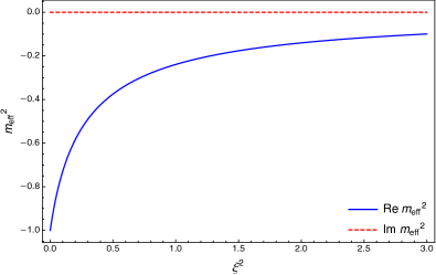
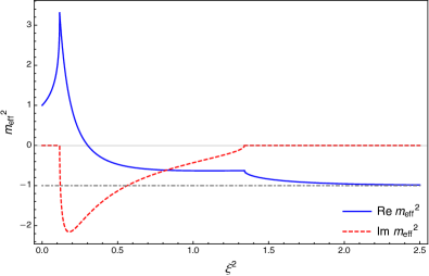
Figure 6: Effective mass-squared as a function of $\xi^{2}$ on the principal branch of the Lambert function. Left: massive theory. Since this represents the unstable vacuum, the mass-squared goes to $-1$ as $\xi\to 0$. The mass-squared is real. Right: tachyonic theory. Since this represents the stable vacuum, the mass-squared goes to $+1$ as $\xi\to 0$. Here, the mass-squared acquires a non-zero imaginary part for a range of values of $\xi$.

As noted before, we have $v_{\text{g}}(\omega)=n(\omega)=v_{\text{p}}(\omega)^{-1}$. The velocities for the massive theory, with $\xi^{2}=0.1$ for illustration, are given are given as a function of frequency in Figure 7. The figure also shows these quantities for the $\xi=0$ theory.

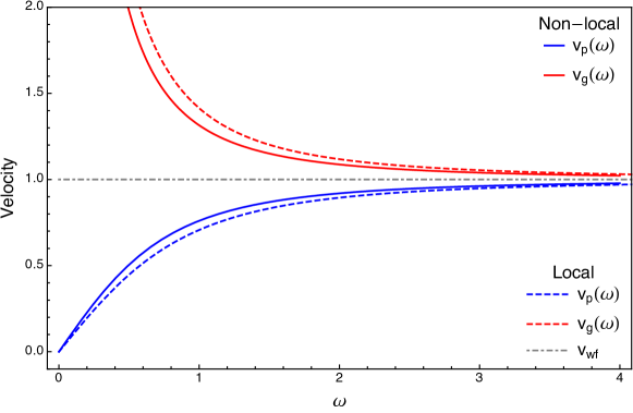
Figure 7: Phase and group velocities for a scalar with $m^{2}>0$ as a function of $\omega$. The continuous lines correspond to the case $\xi^{2}=0.1$ (nonlocal). The dashed lines correspond to $\xi=0$ (local).

The complex effective mass-squared of the tachyonic theory arises because the argument of $W=W_{0}$ is negative and $W_{0}(z)$ has a branch point at $z=-1/e$, and a branch cut extending along the real axis all the way to minus infinity. The nonlocality parameter $\xi_{c}$ at such branch point must satisfy the equation

$$-4\xi_{c}^{2}e^{-2\xi_{c}^{2}}=-\frac{1}{e}\,.$$ (6.23)

This equation admits two real solutions:

$$\xi_{c,1}^{2}:=-\tfrac{1}{2}\,W\left(-\tfrac{1}{2e}\right)\approx 0.116,\qquad\xi_{c,2}^{2}:=-\tfrac{1}{2}\,W_{-1}\left(-\tfrac{1}{2e}\right)\approx 1.339.$$ (6.24)

The behavior of the argument is plotted in Figure 8. For $\xi^{2}$ on the interval $(\xi^{2}_{c,1},\xi^{2}_{c,2})$, the argument of $W_{0}$ is less than $-1/e$ and $W_{0}$ is complex, with positive imaginary part (this corresponds to going above the branch cut). This results in a negative imaginary part for the effective mass-squared. This can be interpreted as attenuation in propagation, because as $\operatorname{Im}W(x)\in[0,\pi]$, we find that the imaginary part of the effective mass satisfies:

$$-\frac{\pi}{2\xi^{2}}\leq\operatorname{Im}m_{\text{eff}}^{2}\leq 0\,,$$ (6.25)

such that

$$\operatorname{Im}n(\omega)^{2}\sim\frac{1}{2\xi^{2}\omega^{2}}>0.$$ (6.26)

If we use the principal branch of the square root, any sign for Im$\,n^{2}(\omega)$ gives $\operatorname{Im}n(\omega)>0$.

In local QFT, the imaginary part of the refractive index must be positive [58, 45, 52] as a consequence of causality of the retarded Green function, analyticity and unitarity. While analyticity properties for nonlocal theories are only partially understood [59, 60, 61] (see [57] for a case where the usual argument fails), it is reassuring to see that we can consistenly work with $\operatorname{Im}n(\omega)>0$ here.

Let us comment briefly on the other solutions with $W_{n}$ and $n\neq 0$. In this case, the solutions are generically complex. The effective mass (6.19), however, is finite for all $n$ and $\xi^{2}>0$, implying that the wavefront velocity is still $v_{\rm wf}=1$ and there is no superluminal propagation. Moreover, given arbitrary finite $\operatorname{Im}n^{2}$ of any sign, we can always take the branch such that $\operatorname{Im}n>0$. This means that any equation of the form $k^{2}=-m_{\text{eff}}^{2}$ is consistent with $\operatorname{Im}n>0$. In Figure 9 we show the $\xi^{2}$ dependence of the effective mass-squared for a solution that uses the branch $W_{-1}$.

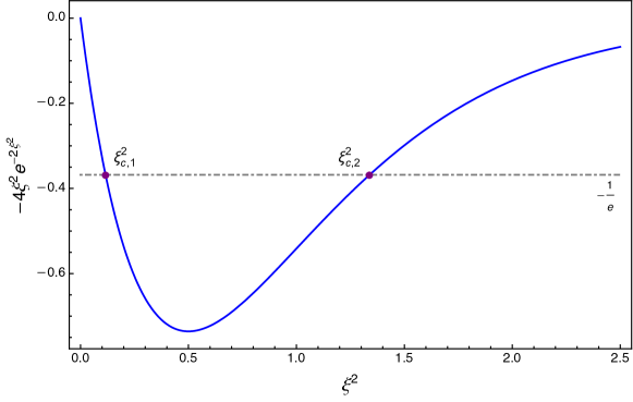
Figure 8: Behavior of the argument of $W$ in (6.19) for the tachyonic theory.

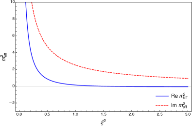
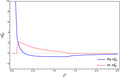
Figure 9: Effective mass-squared as a function of $\xi^{2}$ using the $W_{-1}$ branch of the Lambert function. Left: massive theory. Right: tachyonic theory. In both cases the limit $\xi^{2}\to 0$ does not give the local theory; the mass-squared diverges.

7 Remarks and open questions

We have analyzed nonlocal field theories that appear in string field theory using an effective field theory perspective. We used a derivative expansion of the Lagrangian, and at each order used field redefinitions to adjust the theory and to put it into some canonical form. The results appear to be technically novel and show a set of subtleties and possibilities. We have seen that full locality can be achieved for the purely time-dependent situation and an initial value problem can be formulated for general configurations at the cost of losing manifest Lorentz covariance. Moreover, our analysis suggests, but does not demonstrate, that the theory in question is causal.

There are a number of open questions that could be investigated:

1. It would be significant progress if a closed form expression could be found for the potential $\tilde{V}(\phi;\xi^{2})$ relevant to the purely time-dependent theory. This could require a clever choice for the quasi-symmetry discussed in section 3.3 that is used to simplify the potential. The availability of such a closed form would help settle if the redefinition of the theory is valid non-perturbatively.

2. In a similar vein, it would be useful if some simpler forms or exact subsectors of the redefined Lagrangians were available for the case of fully spacetime dependent configurations. Here, a comparison of the S-matrix elements of the nonlocal and the redefined theory could help—as it allowed us to fix the cubic term in the potential of the redefined theory nonperturbatively.

3. We have argued that the rolling solution in the redefined canonical model poses a puzzle, as it appears to represent the decay and subsequent re-creation of the unstable spacefilling D-brane. This is in sharp contrast with the SFT intuition and evidence that the final state of the tachyon is not the same as the original state. It would be important to confirm that the wild oscillations of the tachyon model map under the redefinition to a smooth rolling solution. At stake is whether the tachyon model captures any of the physics of the string theory. We need to learn how to compute pressure in nonlocal field theory, and test this against the string field theory results. The pressure in rolling solutions does not seem to go to zero, as expected for tachyon matter. Instead, calculations in p-adic theories and the model discussed here (see [22]) exhibit a pressure with ever growing oscillations. It is conceivable that improvements of the stress tensor could change this conclusion.

4. A full investigation of the causality of the original nonlocal (quantum) theory is warranted. A path-integral approach to the question could use a condition derived by Bogoliubov [39] and discussed extensively by Tomboulis [40] as well as ’t Hooft and Veltman [62].

5. An even deeper question asks if our removal of time nonlocalities of the theory, done here perturbatively, is valid beyond perturbation theory and thus defines an equivalent, manifestly causal formulation of the theory. This claim requires two necessary but perhaps not sufficient conditions. One, the redefined theory must be well defined—that is, physically unique. Second, the original nonlocal theory is found to be completely causal, once this analysis can be done reliably. Any progress on this question would help rule out causality troubles in string theory.

References

- [1] R. Pius and A. Sen, “Cutkosky rules for superstring field theory,” JHEP 10, 024 (2016) [erratum: JHEP 09, 122 (2018)] doi:10.1007/JHEP10(2016)024 [arXiv:1604.01783 [hep-th]].
- [2] C. de Lacroix, H. Erbin, S. P. Kashyap, A. Sen and M. Verma, “Closed Superstring Field Theory and its Applications,” Int. J. Mod. Phys. A 32, no.28n29, 1730021 (2017) doi:10.1142/S0217751X17300216 [arXiv:1703.06410 [hep-th]].
- [3] L. Susskind and J. Uglum, “Black hole entropy in canonical quantum gravity and superstring theory,” Phys. Rev. D 50, 2700-2711 (1994) doi:10.1103/PhysRevD.50.2700 [arXiv:hep-th/9401070 [hep-th]]; D. A. Lowe, L. Susskind and J. Uglum, “Information spreading in interacting string field theory,” Phys. Lett. B 327, 226-233 (1994) doi:10.1016/0370-2693(94)90722-6 [arXiv:hep-th/9402136 [hep-th]]; D. A. Lowe, J. Polchinski, L. Susskind, L. Thorlacius and J. Uglum, “Black hole complementarity versus locality,” Phys. Rev. D 52, 6997-7010 (1995) doi:10.1103/PhysRevD.52.6997 [arXiv:hep-th/9506138 [hep-th]].
- [4] D. A. Lowe and A. Strominger, “Strings near a Rindler or black hole horizon,” Phys. Rev. D 51, 1793-1799 (1995) doi:10.1103/PhysRevD.51.1793 [arXiv:hep-th/9410215 [hep-th]].
- [5] J. Polchinski, “String theory and black hole complementarity,” [arXiv:hep-th/9507094 [hep-th]].
- [6] H. Hata, H. Oda and S. Yahikozawa, “String field theory in Rindler space-time and string thermalization,” Prog. Theor. Phys. 96, 985-1020 (1996) doi:10.1143/PTP.96.985 [arXiv:hep-th/9512206 [hep-th]].
- [7] S. B. Giddings, “Locality in quantum gravity and string theory,” Phys. Rev. D 74, 106006 (2006) doi:10.1103/PhysRevD.74.106006 [arXiv:hep-th/0604072 [hep-th]]; S. B. Giddings, D. J. Gross and A. Maharana, “Gravitational effects in ultra high-energy string scattering,” Phys. Rev. D 77, 046001 (2008) doi:10.1103/PhysRevD.77.046001 [arXiv:0705.1816 [hep-th]]; S. B. Giddings, “Nonlocality versus complementarity: A Conservative approach to the information problem,” Class. Quant. Grav. 28, 025002 (2011) doi:10.1088/0264-9381/28/2/025002 [arXiv:0911.3395 [hep-th]]; S. B. Giddings, “Nonviolent nonlocality,” Phys. Rev. D 88, 064023 (2013) doi:10.1103/PhysRevD.88.064023 [arXiv:1211.7070 [hep-th]].
- [8] D. A. Lowe and L. Thorlacius, “Black hole complementarity: The inside view,” Phys. Lett. B 737, 320-324 (2014) doi:10.1016/j.physletb.2014.08.062 [arXiv:1402.4545 [hep-th]].
- [9] M. Dodelson and E. Silverstein, “Long-Range Nonlocality in Six-Point String Scattering: simulation of black hole infallers,” Phys. Rev. D 96, no.6, 066009 (2017) doi:10.1103/PhysRevD.96.066009 [arXiv:1703.10147 [hep-th]]; M. Dodelson and E. Silverstein,“String-theoretic breakdown of effective field theory near black hole horizons,” Phys. Rev. D 96, no.6, 066010 (2017) doi:10.1103/PhysRevD.96.066010 [arXiv:1504.05536 [hep-th]]; A. Mousatov and E. Silverstein, “Recovering Infalling Information via String Spreading,” [arXiv:2002.12377 [hep-th]].
- [10] U. Naseer, “Entanglement Entropy in Closed String Theory,” [arXiv:2002.12148 [hep-th]].
- [11] J. Llosa and J. Vives, “Hamiltonian formalism for nonlocal Lagrangians,” J. Math. Phys. 35, 2856 (1994) doi:10.1063/1.530492; J. Gomis, K. Kamimura and J. Llosa, “Hamiltonian formalism for space-time noncommutative theories,” Phys. Rev. D 63, 045003 (2001) doi:10.1103/PhysRevD.63.045003 [arXiv:hep-th/0006235 [hep-th]].
- [12] J. Gomis, K. Kamimura and T. Ramirez, “Physical degrees of freedom of non-local theories,” Nucl. Phys. B 696, 263-291 (2004) doi:10.1016/j.nuclphysb.2004.06.046 [arXiv:hep-th/0311184 [hep-th]].
- [13] E. T. Tomboulis, “Nonlocal and quasilocal field theories,” Phys. Rev. D 92, no.12, 125037 (2015) doi:10.1103/PhysRevD.92.125037 [arXiv:1507.00981 [hep-th]].
- [14] D. A. Eliezer and R. P. Woodard, “The Problem of Nonlocality in String Theory,” Nucl. Phys. B 325, 389 (1989) doi:10.1016/0550-3213(89)90461-6
- [15] T. Erler and D. J. Gross, “Locality, causality, and an initial value formulation for open string field theory,” [arXiv:hep-th/0406199 [hep-th]].
- [16] T. Erler and H. Matsunaga, “Mapping between Witten and Lightcone String Field Theories,” [arXiv:2012.09521 [hep-th]].
- [17] J. C. Criado and M. Pérez-Victoria, “Field redefinitions in effective theories at higher orders,” JHEP 03, 038 (2019) doi:10.1007/JHEP03(2019)038 [arXiv:1811.09413 [hep-ph]].
- [18] O. Hohm and B. Zwiebach, “Duality invariant cosmology to all orders in ’,” Phys. Rev. D 100, no.12, 126011 (2019) doi:10.1103/PhysRevD.100.126011 [arXiv:1905.06963 [hep-th]].
- [19] N. Moeller and B. Zwiebach, “Dynamics with infinitely many time derivatives and rolling tachyons,” JHEP 10, 034 (2002) doi:10.1088/1126-6708/2002/10/034 [arXiv:hep-th/0207107 [hep-th]].
- [20] N. Moeller and M. Schnabl, “Tachyon condensation in open closed p adic string theory,” JHEP 01, 011 (2004) doi:10.1088/1126-6708/2004/01/011 [arXiv:hep-th/0304213 [hep-th]].
- [21] M. Fujita and H. Hata, “Time dependent solution in cubic string field theory,” JHEP 05, 043 (2003) doi:10.1088/1126-6708/2003/05/043 [arXiv:hep-th/0304163 [hep-th]].
- [22] H. t. Yang, “Stress tensors in p-adic string theory and truncated OSFT,” JHEP 11, 007 (2002) doi:10.1088/1126-6708/2002/11/007 [arXiv:hep-th/0209197 [hep-th]].
- [23] J. A. Minahan, “Quantum corrections in p-adic string theory,” [arXiv:hep-th/0105312 [hep-th]].
- [24] N. Barnaby and N. Kamran, “Dynamics with infinitely many derivatives: The Initial value problem,” JHEP 02, 008 (2008) doi:10.1088/1126-6708/2008/02/008 [arXiv:0709.3968[hep-th]].
- [25] B. Zwiebach, “A Solvable toy model for tachyon condensation in string field theory,” JHEP 09, 028 (2000) doi:10.1088/1126-6708/2000/09/028 [arXiv:hep-th/0008227 [hep-th]].
- [26] A. Sen, “Rolling tachyon,” JHEP 04, 048 (2002) doi:10.1088/1126-6708/2002/04/048 [arXiv:hep-th/0203211 [hep-th]].
- [27] A. Sen, “Tachyon matter,” JHEP 07, 065 (2002) doi:10.1088/1126-6708/2002/07/065 [arXiv:hep-th/0203265 [hep-th]].
- [28] M. Schnabl, “Comments on marginal deformations in open string field theory,” Phys. Lett. B 654, 194-199 (2007) doi:10.1016/j.physletb.2007.08.023 [arXiv:hep-th/0701248 [hep-th]].
- [29] M. Kiermaier, Y. Okawa, L. Rastelli and B. Zwiebach, “Analytic solutions for marginal deformations in open string field theory,” JHEP 01, 028 (2008) doi:10.1088/1126-6708/2008/01/028 [arXiv:hep-th/0701249 [hep-th]].
- [30] M. Kiermaier, Y. Okawa and P. Soler, “Solutions from boundary condition changing operators in open string field theory,” JHEP 03, 122 (2011) doi:10.1007/JHEP03(2011)122 [arXiv:1009.6185 [hep-th]].
- [31] I. Ellwood, “The Closed string tadpole in open string field theory,” JHEP 08, 063 (2008) doi:10.1088/1126-6708/2008/08/063 [arXiv:0804.1131 [hep-th]].
- [32] I. Kishimoto, “Comments on gauge invariant overlaps for marginal solutions in open string field theory,” Prog. Theor. Phys. 120, 875-886 (2008) doi:10.1143/PTP.120.875 [arXiv:0808.0355 [hep-th]].
- [33] M. Kiermaier, Y. Okawa and B. Zwiebach, “The boundary state from open string fields,” [arXiv:0810.1737 [hep-th]].
- [34] M. Kudrna, C. Maccaferri and M. Schnabl, “Boundary State from Ellwood Invariants,” JHEP 07, 033 (2013) doi:10.1007/JHEP07(2013)033 [arXiv:1207.4785 [hep-th]].
- [35] I. Ellwood, “Rolling to the tachyon vacuum in string field theory,” JHEP 12, 028 (2007) doi:10.1088/1126-6708/2007/12/028 [arXiv:0705.0013 [hep-th]].
- [36] S. Hellerman and M. Schnabl, “Light-like tachyon condensation in Open String Field Theory,” JHEP 04, 005 (2013) doi:10.1007/JHEP04(2013)005 [arXiv:0803.1184 [hep-th]].
- [37] T. Erler, T. Masuda and M. Schnabl, “Rolling near the tachyon vacuum,” JHEP 04, 104 (2020) doi:10.1007/JHEP04(2020)104 [arXiv:1902.11103 [hep-th]].
- [38] M. Gutperle and A. Strominger, “Space - like branes,” JHEP 04, 018 (2002) doi:10.1088/1126-6708/2002/04/018 [arXiv:hep-th/0202210 [hep-th]].
- [39] N. N. Bogoliubov and D. V. Shirkov, Fortschr. der Physik, 3 (1955) 439; N. N. Bogoliubov, B. Medvedev and M. Polivanov, ibid, 6 (1958) 169; N. N. Bogoliubov and D. V. Shirkov, Introduction to the theory of quantized fields, Wiley-Interscience (1959).
- [40] E. T. Tomboulis, “Causality and Unitarity via the Tree-Loop Duality Relation,” JHEP 05, 148 (2017) doi:10.1007/JHEP05(2017)148 [arXiv:1701.07052 [hep-th]].
- [41] A. Adams, N. Arkani-Hamed, S. Dubovsky, A. Nicolis, and R. Rattazzi, “Causality, Analyticity and an IR Obstruction to UV Completion,” JHEP, vol. 2006, no. 10, pp. 014–014 (2006) doi: 10.1088/1126-6708/2006/10/014 [hep-th/0602178]
- [42] Y. Aharonov, A. Komar, and L. Susskind, “Superluminal Behavior, Causality, and Instability,” Phys. Rev., vol. 182, no. 5, pp. 1400–1403 (1969), doi: 10.1103/PhysRev.182.1400.
- [43] J. L. Leander, “On the relation between the wavefront speed and the group velocity concept,” The Journal of the Acoustical Society of America, vol. 100, no. 6, pp. 3503–3507, Dec. 1996, doi:10.1121/1.417249.
- [44] G. M. Shore, “Causality and Superluminal Light,” presented at the Time and Matter, Venice, Italy, Feb. 2003 [arxiv:gr-qc/0302116].
- [45] G. M. Shore, “Superluminality and UV Completion,” Nuclear Physics B, vol. 778, no. 3, pp. 219–258, Sep. 2007, doi:10.1016/j.nuclphysb.2007.03.034 [arxiv:hep-th/0701185].
- [46] A. Sen and B. Zwiebach, “Tachyon condensation in string field theory,” JHEP 03, 002 (2000) doi:10.1088/1126-6708/2000/03/002 [arXiv:hep-th/9912249 [hep-th]].
- [47] M. Cho, “Open-closed Hyperbolic String Vertices,” JHEP 05, 046 (2020) doi:10.1007/JHEP05(2020)046 [arXiv:1912.00030 [hep-th]].
- [48] A. H. Fırat, “Hyperbolic three-string vertex,” doi:10.1007/JHEP08(2021)035 [arXiv:2102.03936 [hep-th]].
- [49] L. Brekke, P. G. O. Freund, M. Olson and E. Witten, “Nonarchimedean String Dynamics,” Nucl. Phys. B 302, 365-402 (1988) doi:10.1016/0550-3213(88)90207-6
- [50] J. Halverson, A. Maiti and K. Stoner, “Neural Networks and Quantum Field Theory,” Mach. Learn. Sci. Tech. 2, no.3, 035002 (2021) doi:10.1088/2632-2153/abeca3 [arXiv:2008.08601 [cs.LG]].
- [51] H. Erbin, V. Lahoche and D. O. Samary, “Nonperturbative renormalization for the neural network-QFT correspondence,” [arXiv:2108.01403 [hep-th]].
- [52] C. de Rham and A. J. Tolley, “Causality in Curved Spacetimes: The Speed of Light & Gravity,” Phys. Rev. D, vol. 102, no. 8, p. 084048, Oct. 2020, doi:10.1103/PhysRevD.102.084048 [arxiv:2007.01847].
- [53] C. Armendariz-Picon, T. Damour, and V. Mukhanov, “k-Inflation,” Physics Letters B, vol. 458, no. 2–3, pp. 209–218, Jul. 1999, doi: 10.1016/S0370-2693(99)00603-6 [hep-th/9904075].
- [54] J. Garriga and V. Mukhanov, “Perturbations in k-inflation,” Physics Letters B, vol. 458, no. 2–3, pp. 219–225 (1999), doi: 10.1016/S0370-2693(99)00602-4 [hep-th/9904176].
- [55] E. Babichev, V. Mukhanov, and A. Vikman, “k-Essence, superluminal propagation, causality and emergent geometry,” J. High Energy Phys., vol. 2008, no. 02, pp. 101–101, Feb. 2008, doi:10.1088/1126-6708/2008/02/101 [arxiv:0708.0561].
- [56] N. Brunner, V. Scarani, M. Wegmüller, M. Legré and N. Gisin, “Direct Measurement of Superluminal Group Velocity and Signal Velocity in an Optical Fiber,” Phys. Rev. Lett., vol. 93, issue 20, Nov. 2004, doi:10.1103/PhysRevLett.93.203902 [arXiv:quant-ph/0407155].
- [57] T. J. Hollowood and G. M. Shore, “Causality and Micro-Causality in Curved Spacetime,” Physics Letters B, vol. 655, no. 1–2, pp. 67–74, Oct. 2007, doi: 10.1016/j.physletb.2007.08.073 [0707.2302].
- [58] J. S. Toll, “Causality and the Dispersion Relation: Logical Foundations,” Phys. Rev. 104, 1760-1770 (1956) doi:10.1103/PhysRev.104.1760
- [59] C. De Lacroix, H. Erbin and A. Sen, “Analyticity and Crossing Symmetry of Superstring Loop Amplitudes,” JHEP 05, 139 (2019) doi:10.1007/JHEP05(2019)139 [arXiv:1810.07197 [hep-th]].
- [60] R. Bhattacharya and R. Mahanta, “Analyticity of off-shell Green’s functions in superstring field theory,” JHEP 01, 010 (2021) doi:10.1007/JHEP01(2021)010 [arXiv:2009.03375 [hep-th]].
- [61] R. Bhattacharya and R. Mahanta, “Analyticity Domain for Off-shell Five-point Superstring Loop Amplitudes,” [arXiv:2110.13215 [hep-th]].
- [62] G. ’t Hooft and M. J. G. Veltman, “DIAGRAMMAR,” NATO Sci. Ser. B 4, 177-322 (1974) doi:10.1007/978-1-4684-2826-1_5