Risk-averse Heteroscedastic Bayesian Optimization

Anastasiia Makarova
ETH Zürich
anmakaro@ethz.ch
& Ilnura Usmanova
ETH Zürich
ilnurau@ethz.ch
& Ilija Bogunovic
ETH Zürich
ilijab@ethz.ch
& Andreas Krause
ETH Zürich
krausea@ethz.ch
Abstract

Many black-box optimization tasks arising in high-stakes applications require risk-averse decisions. The standard Bayesian optimization (BO) paradigm, however, optimizes the expected value only. We generalize BO to trade mean and input-dependent variance of the objective, both of which we assume to be unknown a priori. In particular, we propose a novel risk-averse heteroscedastic Bayesian optimization algorithm (RAHBO) that aims to identify a solution with high return and low noise variance, while learning the noise distribution on the fly. To this end, we model both expectation and variance as (unknown) RKHS functions, and propose a novel risk-aware acquisition function. We bound the regret for our approach and provide a robust rule to report the final decision point for applications where only a single solution must be identified. We demonstrate the effectiveness of RAHBO on synthetic benchmark functions and hyperparameter tuning tasks.

1 Introduction

Black-box optimization tasks arise frequently in high-stakes applications such as drug and material discovery [22, 17, 28], genetics [16, 27], robotics [5, 12, 25], hyperparameter tuning of complex learning systems [21, 13, 34], to name a few. In many of these applications, there is often a trade-off between achieving high utility and minimizing risk. Moreover, uncertain and costly evaluations are an inherent part of black-box optimization tasks, and modern learning methods need to handle these aspects when balancing between the previous two objectives.

Bayesian optimization (BO) is a powerful framework for optimizing such costly black-box functions from noisy zeroth-order evaluations. Classical BO approaches are typically risk-neutral as they seek to optimize the expected function value only. In practice, however, two different solutions might attain similar expected function values, but one might produce significantly noisier realizations. This is of major importance when it comes to actual deployment of the found solutions. For example, when selecting hyperparameters of a machine learning algorithm, we might prefer configurations that lead to slightly higher test errors but at the same time lead to smaller variance.

In this paper, we generalize BO to trade off mean and input-dependent noise variance when sequentially querying points and outputting final solutions. We introduce a practical setting where both the black-box objective and input-dependent noise variance are unknown a priori, and the learner needs to estimate them on the fly. We propose a novel optimistic risk-averse algorithm – RAHBO – that makes sequential decisions by simultaneously balancing between exploration (learning about uncertain actions), exploitation (choosing actions that lead to high gains) and risk (avoiding unreliable actions). We bound the cumulative regret of RAHBO as well as the number of samples required to output a single near-optimal risk-averse solution. In our experiments, we demonstrate the risk-averse performance of our algorithm and show that standard BO methods can severely fail in applications where reliability of the reported solutions is of utmost importance.
Refer to caption
(a)
Refer to caption
(b)
Refer to caption
(c)
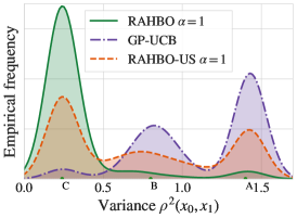
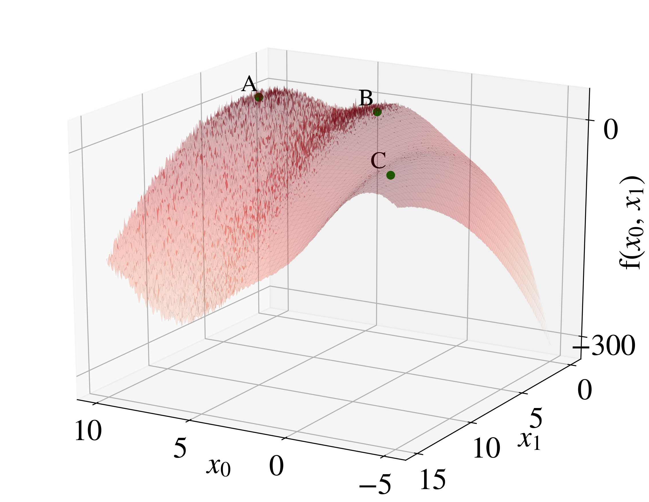
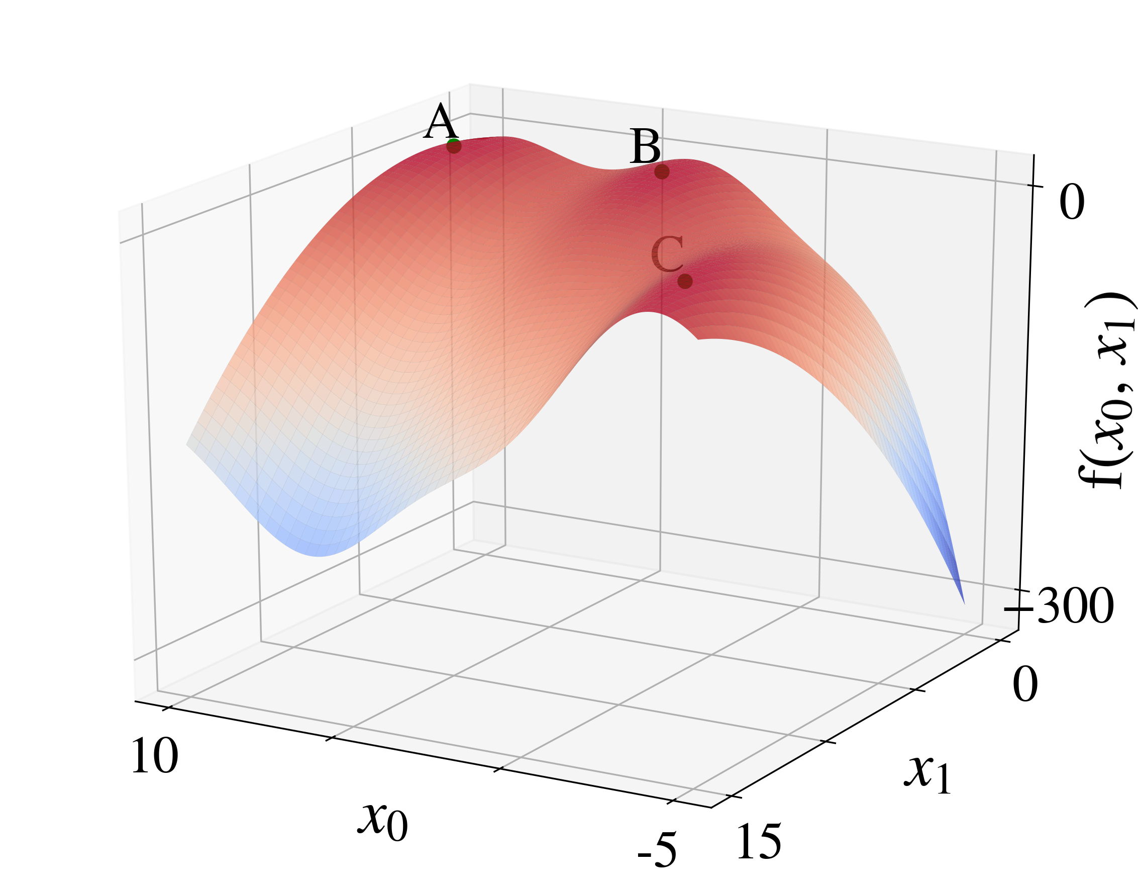
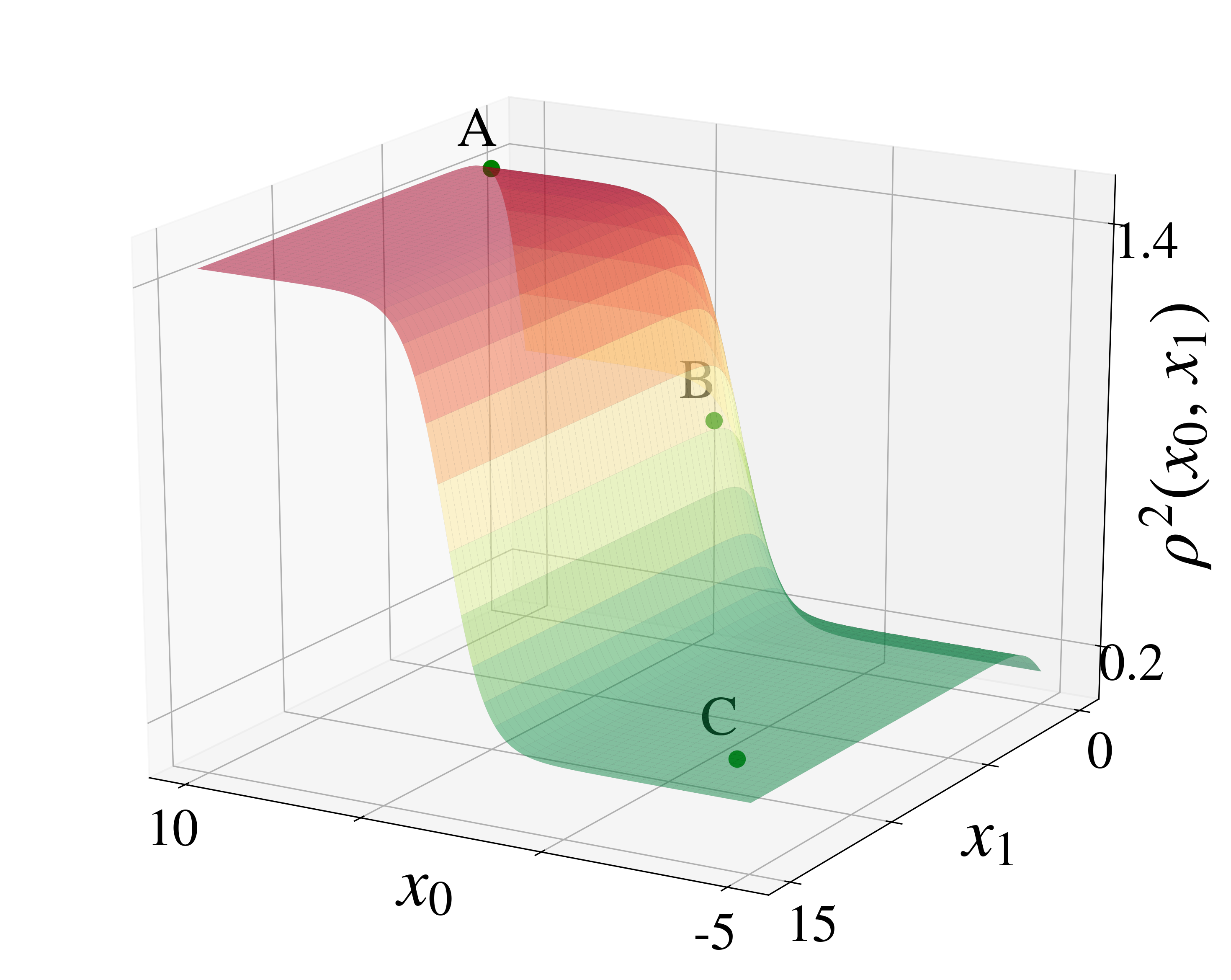
Figure 1: When there is a choice between identical optima with different noise level, standard BO tends to query points corresponding to higher noise. (a) Unknown objective with 3 global maxima marked as (A, B, C); (b) Heteroscedastic noise variance over the same domain: the noise level at (A, B, C) varies according to the sigmoid function; (c) Empirical variance distribution at all points acquired during BO procedure (over 9 experiments with different seeds). The three bumps correspond to the three global optima with different noise variance. RAHBO dominates in choosing the risk-averse optimum, consequently yielding lower risk-averse regret in Figure 5(a).
Related work.

Bayesian optimization (BO) [26] refers to approaches for optimizing a noisy black-box objective that is typically expensive to evaluate. A great number of BO methods have been developed over the years, including a significant number of variants of popular algorithms such as GP-UCB [35], Expected Improvement [26], and Thompson Sampling [14]. While the focus of standard BO approaches is mainly on trading-off exploration vs. exploitation and optimizing for the expected performance, in this work, we additionally focus on the risk that is involved when working with noisy objectives, as illustrated in Figure 1.

The vast majority of previous BO works assume (sub-) Gaussian and homoscedastic noise (i.e., input independent and of some known fixed level). Both assumptions can be restrictive in practice. For example, as demonstrated in [15], the majority of hyperparameter tuning tasks exhibit heteroscedasticity. A few works relax the first assumption and consider, e.g., heavy-tailed noise models [31] and adversarially corrupted observations [8]. The second assumption is typically generalized via heteroscedastic Gaussian process (GP), allowing an explicit dependence of the noise distribution on the evaluation points [6, 10, 7, 20]. Similarly, in this work, we consider heteroscedastic GP models, but unlike the previous works, we specifically focus on the risk that is associated with querying and reporting noisy points.

Several works have recently considered robust and risk-averse aspects in BO. Their central focus is on designing robust strategies and protecting against the change/shift in uncontrollable covariates. They study various notions including worst-case robustness [9], distributional robustness [19, 30], robust mixed strategies [33] and other notions of risk-aversion [18, 11, 29], and while some of them report robust regret guarantees, their focus is primarily on the robustness in the homoscedastic GP setting. Instead, in our setting, we account for the risk that comes from the realization of random noise with unknown distribution. Rather than optimizing the expected performance, in our risk-averse setting, we prefer inputs with lower variance. To this end, we incorporate the learning of the noise distribution into the optimization procedure via a mean-variance objective. The closest to our setting is risk-aversion with respect to noise in multi-armed bandits [32]. Their approach, however, fails to exploit correlation in rewards among similar arms.

Contributions.

We propose a novel Risk-averse Heteroscedastic Bayesian optimization (RAHBO) approach based on the optimistic principle that trades off the expectation and uncertainty of the mean-variance objective function. We model both the objective and variance as (unknown) functions belonging to RKHS space of functions, and propose a practical risk-aware algorithm in the heteroscedastic GP setting. In our theoretical analysis, we establish rigorous sublinear regret guarantees for our algorithm, and provide a robust reporting rule for applications where only a single solution is required. We demonstrate the effectiveness of RAHBO on synthetic benchmarks, as well as on hyperparameter tuning tasks for the Swiss free-electron laser and a machine learning model.

2 Problem setting

Let 𝒳𝒳\mathcal{X} be a given compact set of inputs (𝒳d𝒳superscript𝑑\mathcal{X}\subset\mathbb{R}^{d} for some d𝑑d\in\mathbb{N}). We consider a problem of sequentially interacting with a fixed and unknown objective f:𝒳:𝑓𝒳f:\mathcal{X}\rightarrow\mathbb{R}. At every round of this procedure, the learner selects an action xt𝒳subscript𝑥𝑡𝒳x_{t}\in\mathcal{X}, and obtains a noisy observation

yt=f(xt)+ξ(xt),subscript𝑦𝑡𝑓subscript𝑥𝑡𝜉subscript𝑥𝑡y_{t}=f(x_{t})+\xi(x_{t}), (1)

where ξ(xt)𝜉subscript𝑥𝑡\xi(x_{t}) is zero-mean noise independent across different time steps t𝑡t. In this work, we consider sub-Gaussian heteroscedastic noise that depends on the query location.

Definition 1.

A zero-mean real-valued random variable ξ𝜉\xi is ρ𝜌\rho–sub-Gaussian, if there exists variance-proxy ρ2superscript𝜌2\rho^{2} such that λ,𝔼[eλξ]eλ2ρ22formulae-sequencefor-all𝜆𝔼delimited-[]superscript𝑒𝜆𝜉superscript𝑒superscript𝜆2superscript𝜌22\forall\lambda\in\mathbb{R},\ \ \mathbb{E}[e^{\lambda\xi}]\leq e^{\frac{\lambda^{2}\rho^{2}}{2}}.

For a sub-Gaussian ξ𝜉\xi, its variance 𝕍ar[ξ]𝕍𝑎𝑟delimited-[]𝜉\mathbb{V}ar[\xi] lower bounds any valid variance-proxy ρ𝜌\rho, i.e., 𝕍ar[ξ]ρ2𝕍𝑎𝑟delimited-[]𝜉superscript𝜌2\mathbb{V}ar[\xi]\leq\rho^{2}. In case 𝕍ar[ξ]=ρ2𝕍𝑎𝑟delimited-[]𝜉superscript𝜌2\mathbb{V}ar[\xi]=\rho^{2} holds, ξ𝜉\xi is said to be strictly ρ𝜌\rho–sub-Gaussian. Besides zero-mean Gaussian random variables, most standard symmetric bounded random variables (e.g., Bernoulli, beta, uniform, binomial) are strictly sub-Gaussian (see [2, Proposition 1.1]). Throughout the paper, we consider sub-Gaussian noise, and in Section 3.3, we specialize to the case of strictly sub-Gaussian noise.

Optimization objective. Unlike the previous works that mostly focus on sequential optimization of f𝑓f in the homoscedastic noise case, in this work, we consider the trade-off between risk and return in the heteroscedastic case. While there exist a number of risk-averse objectives, we consider the simple and frequently used mean-variance objective (MV) [32]. Here, the objective value at x𝒳𝑥𝒳x\in\mathcal{X} is a trade-off between the (mean) return f(x)𝑓𝑥f(x) and the risk expressed by its variance-proxy ρ2(x)superscript𝜌2𝑥\rho^{2}(x):

MV(x)=f(x)αρ2(x),MV𝑥𝑓𝑥𝛼superscript𝜌2𝑥\displaystyle\text{MV}(x)=f(x)-\alpha\rho^{2}(x), (2)

where α0𝛼0\alpha\geq 0 is a so-called coefficient of absolute risk tolerance. In this work, we assume α𝛼\alpha is fixed and known to the learner. In the case of α=0𝛼0\alpha=0, maximizing MV(x)MV𝑥\text{MV}(x) coincides with the standard BO objective.

Performance metrics. We aim to construct a sequence of input evaluations xtsubscript𝑥𝑡x_{t} that eventually maximizes the risk-averse objective MV(x)MV𝑥\text{MV}(x). To assess this convergence, we consider two metrics. The first metric corresponds to the notion of cumulative regret similar to the one used in standard BO and bandits. Here, the learner’s goal is to maximize its risk-averse cumulative reward over a time horizon T𝑇T, or equivalently minimize its risk-averse cumulative regret:

RT=t=1T[MV(x)MV(xt)],subscript𝑅𝑇superscriptsubscript𝑡1𝑇delimited-[]MVsuperscript𝑥MVsubscript𝑥𝑡R_{T}=\sum_{t=1}^{T}\Bigl{[}\text{MV}(x^{*})-\text{MV}(x_{t})\Bigr{]}, (3)

where xargmaxx𝒳MV(x)superscript𝑥subscript𝑥𝒳MV𝑥x^{*}\in\arg\max_{x\in\mathcal{X}}\text{MV}(x). A sublinear growth of RTsubscript𝑅𝑇R_{T} with T𝑇T implies vanishing average regret RT/T0subscript𝑅𝑇𝑇0R_{T}/T\rightarrow 0 as T𝑇T\rightarrow\infty. Intuitively, this implies the existence of some t𝑡t such that MV(xt)MVsubscript𝑥𝑡\text{MV}(x_{t}) is arbitrarily close to the optimal value MV(x)MVsuperscript𝑥\text{MV}(x^{*}).

The second metric is used when the learner seeks to simultaneously minimize the number of expensive function evaluations T𝑇T. Namely, for a given accuracy ϵ0italic-ϵ0\epsilon\geq 0, we report a single "good" risk-averse point x^T𝒳subscript^𝑥𝑇𝒳\hat{x}_{T}\in\mathcal{X} after a total of T𝑇T rounds, that satisfies:

MV(x^T)MV(x)ϵ.MVsubscript^𝑥𝑇MVsuperscript𝑥italic-ϵ\text{MV}(\hat{x}_{T})\geq\text{MV}(x^{*})-\epsilon. (4)

Both metrics are important for choosing risk-averse solutions and which one is preferred depends on the application at hand. For example, risk-averse cumulative regret RTsubscript𝑅𝑇R_{T} might be of a greater interest in online recommendation systems, while reporting a single point with high MV value might be more suitable when tuning machine learning hyperparameters. We consider both performance metrics in our experiments.

Regularity assumptions. We consider standard smoothness assumptions [35, 9] when it comes to the unknown function f:𝒳:𝑓𝒳f:\mathcal{X}\rightarrow\mathbb{R}. In particular, we assume that f()𝑓f(\cdot) belongs to a reproducing kernel Hilbert space (RKHS) κsubscript𝜅\mathcal{H}_{\kappa} (a space of smooth and real-valued functions defined on 𝒳𝒳\mathcal{X}), i.e., fκ𝑓subscript𝜅f\in\mathcal{H}_{\kappa}, induced by a kernel function κ(,)𝜅\kappa(\cdot,\cdot). We also assume that κ(x,x)1𝜅𝑥superscript𝑥1\kappa(x,x^{\prime})\leq 1 for every x,x𝒳𝑥superscript𝑥𝒳x,x^{\prime}\in\mathcal{X}. Moreover, the RKHS norm of f()𝑓f(\cdot) is assumed to be bounded fκfsubscriptnorm𝑓𝜅subscript𝑓\|f\|_{\kappa}\leq\mathcal{B}_{f} for some fixed constant f>0subscript𝑓0\mathcal{B}_{f}>0. We assume that the noise ξ(x)𝜉𝑥\xi(x) is ρ(x)𝜌𝑥\rho(x)–sub-Gaussian with variance-proxy ρ2(x)superscript𝜌2𝑥\rho^{2}(x) uniformly bounded ρ(x)[ϱ¯,ϱ¯]𝜌𝑥¯italic-ϱ¯italic-ϱ\rho(x)\in[\smash{\underline{\varrho}},\bar{\varrho}] for some constant values ϱ¯ϱ¯>0¯italic-ϱ¯italic-ϱ0\bar{\varrho}\geq\smash{\underline{\varrho}}>0.

3 Algorithms

We first recall the Gaussian process (GP) based framework for sequential learning of RKHS functions from observations with heteroscedastic noise. Then, in Section 3.2, we consider a simple risk-averse Bayesian optimization problem with known variance-proxy, and later on in Section 3.3, we focus on our main problem setting in which the variance-proxy is unknown.

3.1 Bayesian optimization with heteroscedastic noise

Before addressing the risk-averse objective, we briefly recall the standard GP-UCB algorithm [35] in the setting of heteroscedastic sub-Gaussian noise. The regularity assumptions permit the construction of confidence bounds via GP model. Particularly, to decide which point to query at every round, GP-UCB makes use of the posterior GP mean and variance denoted by μt()subscript𝜇𝑡\mu_{t}(\cdot) and σt2()subscriptsuperscript𝜎2𝑡\sigma^{2}_{t}(\cdot), respectively. They are computed based on the previous measurements y1:t=[y1,,yt]subscript𝑦:1𝑡superscriptsubscript𝑦1subscript𝑦𝑡topy_{1:t}=[y_{1},\dots,y_{t}]^{\top} and the given kernel κ(,)𝜅\kappa(\cdot,\cdot) :

μt(x)=κt(x)T(Kt+λΣt)1y1:t,subscript𝜇𝑡𝑥subscript𝜅𝑡superscript𝑥𝑇superscriptsubscript𝐾𝑡𝜆subscriptΣ𝑡1subscript𝑦:1𝑡\displaystyle\mu_{t}(x)=\kappa_{t}(x)^{T}(K_{t}+\lambda\Sigma_{t})^{-1}y_{1:t}, (5)
σt2(x)=1λ(κ(x,x)κt(x)(Kt+λΣt)1κt(x)),subscriptsuperscript𝜎2𝑡𝑥1𝜆𝜅𝑥𝑥subscript𝜅𝑡superscript𝑥topsuperscriptsubscript𝐾𝑡𝜆subscriptΣ𝑡1subscript𝜅𝑡𝑥\displaystyle\sigma^{2}_{t}(x)=\frac{1}{\lambda}\big{(}\kappa(x,x)-\kappa_{t}(x)^{\top}(K_{t}+\lambda\Sigma_{t})^{-1}\kappa_{t}(x)\big{)}, (6)

where Σt:=diag(ρ2(x1),,ρ2(xt))assignsubscriptΣ𝑡diagsuperscript𝜌2subscript𝑥1superscript𝜌2subscript𝑥𝑡\Sigma_{t}:=\text{diag}(\rho^{2}(x_{1}),\dots,\rho^{2}(x_{t})), (Kt)i,j=κ(xi,xj),κt(x)T=[κ(x1,x),,κ(xt,x)]Tformulae-sequencesubscriptsubscript𝐾𝑡𝑖𝑗𝜅subscript𝑥𝑖subscript𝑥𝑗subscript𝜅𝑡superscript𝑥𝑇superscript𝜅subscript𝑥1𝑥𝜅subscript𝑥𝑡𝑥𝑇(K_{t})_{i,j}=\kappa(x_{i},x_{j}),\ \kappa_{t}(x)^{T}=[\kappa(x_{1},x),\dots,\kappa(x_{t},x)]^{T}, λ>0𝜆0\lambda>0 and prior modelling assumptions are ξ()𝒩(0,ρ2())similar-to𝜉𝒩0superscript𝜌2\xi(\cdot)\sim\mathcal{N}(0,\rho^{2}(\cdot)) and fGP(0,λ1κ)similar-to𝑓𝐺𝑃0superscript𝜆1𝜅f\sim GP(0,\lambda^{-1}\kappa).

At time t𝑡t, GP-UCB maximizes the upper confidence bound of f()𝑓f(\cdot), i.e.,

xtargmaxx𝒳μt1(x)+βtσt1(x)=:ucbtf(x).subscript𝑥𝑡subscriptargmax𝑥𝒳subscriptsubscript𝜇𝑡1𝑥subscript𝛽𝑡subscript𝜎𝑡1𝑥:absentsubscriptsuperscriptucb𝑓𝑡𝑥\displaystyle x_{t}\in\operatorname*{arg\,max}_{x\in\mathcal{X}}\;\underbrace{\mu_{t-1}(x)+\beta_{t}\sigma_{t-1}(x)}_{=:\mathrm{ucb}^{f}_{t}(x)}. (7)

If the noise ξt(xt)subscript𝜉𝑡subscript𝑥𝑡\xi_{t}(x_{t}) is heteroscedastic and ρ(xt)𝜌subscript𝑥𝑡\rho(x_{t})-sub-Gaussian, the following confidence bounds hold:

Lemma 1 (Lemma 7 in [20]).

Let fκ𝑓subscript𝜅f\in\mathcal{H}_{\kappa}, and μt()subscript𝜇𝑡\mu_{t}(\cdot) and σt2()subscriptsuperscript𝜎2𝑡\sigma^{2}_{t}(\cdot) be defined as in Eqs. 5 and 6 with λ>0.𝜆0\lambda>0. Assume that the observations (xt,yt)t1subscriptsubscript𝑥𝑡subscript𝑦𝑡𝑡1(x_{t},y_{t})_{t\geq 1} satisfy Eq. 1. Then the following holds for all t1𝑡1t\geq 1 and x𝒳𝑥𝒳x\in\mathcal{X} with probability at least 1δ1𝛿1-\delta:

|μt1(x)f(x)|(2ln(det(λΣt+Kt)1/2δdet(λΣt)1/2)+λfκ):=βtσt1(x).\displaystyle|\mu_{t-1}(x)-f(x)|\leq\underbrace{\Bigg{(}\sqrt{2\ln\bigg{(}\frac{\det(\lambda\Sigma_{t}+K_{t})^{1/2}}{\delta\det(\lambda\Sigma_{t})^{1/2}}}\bigg{)}+\sqrt{\lambda}\|f\|_{\kappa}\Bigg{)}}_{:=\beta_{t}}\sigma_{t-1}(x). (8)

Here, βtsubscript𝛽𝑡\beta_{t} stands for the parameter that balances between exploration vs. exploitation and ensures the validity of confidence bounds. The analogous concentration inequalities in case of homoscedastic noise were considered in [1, 14, 35].

Failure of GP-UCB in the risk-averse setting. GP-UCB is guaranteed to achieve sublinear cumulative regret with high probability in the risk-neutral (homoscedastic/heteroscedastic) BO setting [35, 14]. However, for the risk-averse setting in Eq. 2, the maximizers xargmaxx𝒳MV(x)superscript𝑥subscriptargmax𝑥𝒳MV𝑥x^{*}\in\operatorname*{arg\,max}_{x\in\mathcal{X}}\text{MV}(x) and xfargmaxx𝒳f(x)subscriptsuperscript𝑥𝑓subscriptargmax𝑥𝒳𝑓𝑥x^{*}_{f}\in\operatorname*{arg\,max}_{x\in\mathcal{X}}f(x) might not coincide, and consequently, MV(x)MVsuperscript𝑥\text{MV}(x^{*}) can be significantly larger than MV(xf)MVsubscriptsuperscript𝑥𝑓\text{MV}(x^{*}_{f}). This is illustrated in Figure 1, where GP-UCB most frequently chooses optimum A𝐴A of the highest risk.

3.2 Warm up: Known variance-proxy

We remedy the previous issue with GP-UCB by proposing a natural Risk-averse Heteroscedastic BO (RAHBO) in case of the known variance-proxy ρ2()superscript𝜌2\rho^{2}(\cdot). At each round t𝑡t, RAHBO chooses the action:

xtargmaxx𝒳μt1(x)+βtσt1(x)αρ2(x),subscript𝑥𝑡subscriptargmax𝑥𝒳subscript𝜇𝑡1𝑥subscript𝛽𝑡subscript𝜎𝑡1𝑥𝛼superscript𝜌2𝑥x_{t}\in\operatorname*{arg\,max}_{x\in\mathcal{X}}\;\mu_{t-1}(x)+\beta_{t}\sigma_{t-1}(x)-\alpha\rho^{2}(x), (9)

where βtsubscript𝛽𝑡\beta_{t} is from Lemma 1 and α𝛼\alpha is from Eq. 2. In the next section, we further relax the assumption of the variance-proxy and consider a more practical setting when ρ2()superscript𝜌2\rho^{2}(\cdot) is unknown to the learner. For the current setting, the performance of RAHBO is formally captured in the following proposition.

Proposition 1.

Consider any fκ𝑓subscript𝜅f\in\mathcal{H}_{\kappa} with fκfsubscriptnorm𝑓𝜅subscript𝑓\|f\|_{\kappa}\leq\mathcal{B}_{f} and sampling model from Eq. 1 with known variance-proxy ρ2(x)superscript𝜌2𝑥\rho^{2}(x). Let {βt}t=1Tsuperscriptsubscriptsubscript𝛽𝑡𝑡1𝑇\{\beta_{t}\}_{t=1}^{T} be set as in Lemma 1 with λ=1𝜆1\lambda=1. Then, with probability at least 1δ1𝛿1-\delta, RAHBO attains cumulative risk-averse regret RT=𝒪(βTTγT(ϱ¯2+1))subscript𝑅𝑇𝒪subscript𝛽𝑇𝑇subscript𝛾𝑇superscript¯italic-ϱ21R_{T}=\mathcal{O}\big{(}\beta_{T}\sqrt{T\gamma_{T}(\bar{\varrho}^{2}+1)}\big{)}.

Here, γTsubscript𝛾𝑇\gamma_{T} denotes the maximum information gain [35] at time T𝑇T defined via mutual information I(y1:T,f1:T)𝐼subscript𝑦:1𝑇subscript𝑓:1𝑇I(y_{1:T},f_{1:T}) between evaluations y1:Tsubscript𝑦:1𝑇y_{1:T} and f1:T=[f(x1),,f(xT)]subscript𝑓:1𝑇superscript𝑓subscript𝑥1𝑓subscript𝑥𝑇topf_{1:T}=[f(x_{1}),\dots,f(x_{T})]^{\top} at points AD𝐴𝐷A\subset D:

γT:=maxA𝒳,|A|=TI(y1:T,f1:T),assignsubscript𝛾𝑇formulae-sequence𝐴𝒳𝐴𝑇𝐼subscript𝑦:1𝑇subscript𝑓:1𝑇\displaystyle\gamma_{T}:=\underset{A\subset\mathcal{X},\;|A|=T}{\max}\;I(y_{1:T},f_{1:T}), (10)
whereI(y1:T,f1:T)=12t=1Tln(1+σt12(xt)ρ2(xt))where𝐼subscript𝑦:1𝑇subscript𝑓:1𝑇12superscriptsubscript𝑡1𝑇1superscriptsubscript𝜎𝑡12subscript𝑥𝑡superscript𝜌2subscript𝑥𝑡\displaystyle\text{where}\ \ I(y_{1:T},f_{1:T})=\frac{1}{2}\sum_{t=1}^{T}\ln\Big{(}1+\tfrac{\sigma_{t-1}^{2}(x_{t})}{\rho^{2}(x_{t})}\Big{)} (11)

in case of heteroscedastic noise (see Section A.1.1). The upper bounds on γTsubscript𝛾𝑇\gamma_{T} are provided in [35] widely used kernels. These upper bounds typically scale sublinearly in T𝑇T; for linear kernel γT=𝒪(dlogT)subscript𝛾𝑇𝒪𝑑𝑇\gamma_{T}=\mathcal{O}(d\log T), and in case of squared exponential kernel γT=𝒪(d(logT)d+1)subscript𝛾𝑇𝒪𝑑superscript𝑇𝑑1\gamma_{T}=\mathcal{O}(d(\log T)^{d+1}). While these bounds are derived assuming the homoscedastic GP setting with some fixed constant noise variance, we show (in Section A.1.3) that the same rates (up to a multiplicative constant factor) apply in the heteroscedastic case.

3.3 RAHBO for unknown variance-proxy

In the case of unknown variance-proxy, the confidence bounds for the unknown f(x)𝑓𝑥f(x) in Lemma 1 can not be readily used, and we construct new ones on the combined mean-variance objective. To learn about the unknown ρ2(x)superscript𝜌2𝑥\rho^{2}(x), we make some further assumptions.

Assumption 1.

The variance-proxy ρ2(x)superscript𝜌2𝑥\rho^{2}(x) belongs to an RKHS induced by some kernel κvarsuperscript𝜅𝑣𝑎𝑟\kappa^{var}, i.e., ρ2κvarsuperscript𝜌2subscriptsuperscript𝜅𝑣𝑎𝑟\rho^{2}\in\mathcal{H}_{\kappa^{var}}, and its RKHS norm is bounded ρ2κvarvarsubscriptnormsuperscript𝜌2superscript𝜅𝑣𝑎𝑟subscript𝑣𝑎𝑟\|\rho^{2}\|_{\kappa^{var}}\leq\mathcal{B}_{var} for some finite var>0subscript𝑣𝑎𝑟0\mathcal{B}_{var}>0. Moreover, the noise ξ(x)𝜉𝑥\xi(x) in Eq. 1 is strictly ρ(x)𝜌𝑥\rho(x)–sub-Gaussian, i.e., 𝕍ar[ξ(x)]=ρ2(x)𝕍𝑎𝑟delimited-[]𝜉𝑥superscript𝜌2𝑥\mathbb{V}ar[\xi(x)]=\rho^{2}(x) for every x𝒳𝑥𝒳x\in\mathcal{X}.

As a consequence of our previous assumption, we can now focus on estimating the variance since 𝕍ar[ξ()]𝕍𝑎𝑟delimited-[]𝜉\mathbb{V}ar[\xi(\cdot)] and ρ2()superscript𝜌2\rho^{2}(\cdot) coincide. In particular, to estimate 𝕍ar[ξ()]𝕍𝑎𝑟delimited-[]𝜉\mathbb{V}ar[\xi(\cdot)] we consider a repeated experiment setting, where for each xtsubscript𝑥𝑡x_{t} we collect k>1𝑘1k>1 evaluations {yi(xt)}i=1ksuperscriptsubscriptsubscript𝑦𝑖subscript𝑥𝑡𝑖1𝑘\{y_{i}(x_{t})\}_{i=1}^{k}, yi(xt)=f(xt)+ξi(xt)subscript𝑦𝑖subscript𝑥𝑡𝑓subscript𝑥𝑡subscript𝜉𝑖subscript𝑥𝑡y_{i}(x_{t})=f(x_{t})+\xi_{i}(x_{t}). Then, the sample mean and variance of ξ(xt)𝜉subscript𝑥𝑡\xi(x_{t}) are given as:

m^k(xt)=1ki=1kyi(xt)ands^k2(xt)=1k1i=1k(yi(xt)m^k(xt))2.formulae-sequencesubscript^𝑚𝑘subscript𝑥𝑡1𝑘superscriptsubscript𝑖1𝑘subscript𝑦𝑖subscript𝑥𝑡andsubscriptsuperscript^𝑠2𝑘subscript𝑥𝑡1𝑘1superscriptsubscript𝑖1𝑘superscriptsubscript𝑦𝑖subscript𝑥𝑡subscript^𝑚𝑘subscript𝑥𝑡2\hat{m}_{k}(x_{t})=\frac{1}{k}\sum_{i=1}^{k}y_{i}(x_{t})\quad\text{and}\quad\hat{s}^{2}_{k}(x_{t})=\frac{1}{k-1}\sum_{i=1}^{k}\big{(}y_{i}(x_{t})-\hat{m}_{k}(x_{t})\big{)}^{2}. (12)

The key idea is that for strictly sub-Gaussian noise ξ(x)𝜉𝑥\xi(x), s^1:t2=[s^k2(x1),,s^k2(xt)]subscriptsuperscript^𝑠2:1𝑡superscriptsubscriptsuperscript^𝑠2𝑘subscript𝑥1subscriptsuperscript^𝑠2𝑘subscript𝑥𝑡top\hat{s}^{2}_{1:t}=[\hat{s}^{2}_{k}(x_{1}),\dots,\hat{s}^{2}_{k}(x_{t})]^{\top} yields unbiased, but noisy evaluations of the unknown variance-proxy ρ1:t2=[ρ2(x1),,ρ2(xt)]subscriptsuperscript𝜌2:1𝑡superscriptsuperscript𝜌2subscript𝑥1superscript𝜌2subscript𝑥𝑡top\rho^{2}_{1:t}=[\rho^{2}(x_{1}),\dots,\rho^{2}(x_{t})]^{\top}, i.e.,

s^k2(xt)=ρ2(xt)+η(xt)subscriptsuperscript^𝑠2𝑘subscript𝑥𝑡superscript𝜌2subscript𝑥𝑡𝜂subscript𝑥𝑡\hat{s}^{2}_{k}(x_{t})=\rho^{2}(x_{t})+\eta(x_{t}) (13)

with zero-mean noise η(xt)𝜂subscript𝑥𝑡\eta(x_{t}). In order to efficiently estimate ρ2()superscript𝜌2\rho^{2}(\cdot), we need an additional assumption.

Assumption 2.

The noise η(x)𝜂𝑥\eta(x) in Eq. 13 is ρη(x)subscript𝜌𝜂𝑥\rho_{\eta}(x)–sub-Gaussian with known ρη2(x)superscriptsubscript𝜌𝜂2𝑥\rho_{\eta}^{2}(x) and the realizations {η(xt)}t1subscript𝜂subscript𝑥𝑡𝑡1\{\eta(x_{t})\}_{t\geq 1} are independent between t𝑡t.

We note that a similar assumption is made in [32] in the multi-armed bandit setting. The fact that ρη2()subscriptsuperscript𝜌2𝜂\rho^{2}_{\eta}(\cdot) is known is rather mild as Assumption 1 allows controlling its value. For example, in case of strictly sub-Gaussian η(x)𝜂𝑥\eta(x) we show (in Section A.2) that 𝕍ar[η()]=ρη2()2ρ4()/(k1)𝕍𝑎𝑟delimited-[]𝜂subscriptsuperscript𝜌2𝜂2superscript𝜌4𝑘1\mathbb{V}ar[\eta(\cdot)]=\rho^{2}_{\eta}(\cdot)\leq 2\rho^{4}(\cdot)/(k-1). Then, given that ρ2()ϱ¯2superscript𝜌2superscript¯italic-ϱ2\rho^{2}(\cdot)\leq\bar{\varrho}^{2}, we can utilize the following (rather conservative) bound as a variance-proxy, i.e., ρη2(x)=2ϱ¯4/(k1)superscriptsubscript𝜌𝜂2𝑥2superscript¯italic-ϱ4𝑘1\rho_{\eta}^{2}(x)=2\bar{\varrho}^{4}/(k-1).

Algorithm 1 Risk-averse Heteroscedastic Bayesian Optimization (RAHBO)
0:  Parameters α,{βt,βtvar}t1,λ𝛼subscriptsubscript𝛽𝑡superscriptsubscript𝛽𝑡𝑣𝑎𝑟𝑡1𝜆\alpha,\{\beta_{t},\beta_{t}^{var}\}_{t\geq 1},\lambda, k𝑘k, Prior μ0f=μ0var=0superscriptsubscript𝜇0𝑓superscriptsubscript𝜇0𝑣𝑎𝑟0\mu_{0}^{f}=\mu_{0}^{var}=0, Kernel functions κ,κvar𝜅superscript𝜅𝑣𝑎𝑟\kappa,\kappa^{var}
1:  for t=1,2,𝑡12t=1,2,\ldots do
2:     Construct confidence bounds ucbtvar()superscriptsubscriptucb𝑡𝑣𝑎𝑟\mathrm{ucb}_{t}^{var}(\cdot) and lcbtvar()superscriptsubscriptlcb𝑡𝑣𝑎𝑟\mathrm{lcb}_{t}^{var}(\cdot) as in Eqs. 14 and 15
3:     Construct ucbtf()subscriptsuperscriptucb𝑓𝑡\mathrm{ucb}^{f}_{t}(\cdot) as in Eq. 7
4:     Select xtargmaxx𝒳ucbtf(x)αlcbtvar(x)subscript𝑥𝑡subscriptargmax𝑥𝒳subscriptsuperscriptucb𝑓𝑡𝑥𝛼superscriptsubscriptlcb𝑡𝑣𝑎𝑟𝑥x_{t}\in\operatorname*{arg\,max}_{x\in\mathcal{X}}\mathrm{ucb}^{f}_{t}(x)-\alpha\;\mathrm{lcb}_{t}^{var}(x)
5:     Observe k𝑘k samples: yi(xt)=f(xt)+ξi(xt)for everyi[k]formulae-sequencesubscript𝑦𝑖subscript𝑥𝑡𝑓subscript𝑥𝑡subscript𝜉𝑖subscript𝑥𝑡for every𝑖delimited-[]𝑘y_{i}(x_{t})=f(x_{t})+\xi_{i}(x_{t})\quad\text{for every}\quad i\in[k]
6:     Use samples {yi(xt)}i=1ksuperscriptsubscriptsubscript𝑦𝑖subscript𝑥𝑡𝑖1𝑘\{y_{i}(x_{t})\}_{i=1}^{k} to compute sample mean m^k(xt)subscript^𝑚𝑘subscript𝑥𝑡\hat{m}_{k}(x_{t}) and variance s^k2(xt)subscriptsuperscript^𝑠2𝑘subscript𝑥𝑡\hat{s}^{2}_{k}(x_{t}) as in Eq. 12
7:     Use xt,s^k2(xt)subscript𝑥𝑡superscriptsubscript^𝑠𝑘2subscript𝑥𝑡x_{t},\hat{s}_{k}^{2}(x_{t}) to update posterior μtvar()superscriptsubscript𝜇𝑡𝑣𝑎𝑟\mu_{t}^{var}(\cdot) and σtvar()superscriptsubscript𝜎𝑡𝑣𝑎𝑟\sigma_{t}^{var}(\cdot) as in Eqs. 32 and 33
8:     Use ucbtvar()superscriptsubscriptucb𝑡𝑣𝑎𝑟\mathrm{ucb}_{t}^{var}(\cdot) to compute Σ^tsubscript^Σ𝑡\hat{\Sigma}_{t} as in Eq. 16
9:     Use xt,m^k(xt)subscript𝑥𝑡subscript^𝑚𝑘subscript𝑥𝑡x_{t},\hat{m}_{k}(x_{t}) and Σ^tsubscript^Σ𝑡\hat{\Sigma}_{t} to update posterior μt()subscript𝜇𝑡\mu_{t}(\cdot) and σt()subscript𝜎𝑡\sigma_{t}(\cdot) as in Eqs. 5 and 6
10:  end for

RAHBO algorithm. We present our Risk-averse Heteroscedastic BO approach for unknown variance-proxy in Algorithm 1. Our method relies on building the following two GP models.

Firstly, we use sample variance evaluations s^1:t2subscriptsuperscript^𝑠2:1𝑡\hat{s}^{2}_{1:t} to construct a GP model for ρ2()superscript𝜌2\rho^{2}(\cdot). The corresponding μt1var()subscriptsuperscript𝜇𝑣𝑎𝑟𝑡1\mu^{var}_{t-1}(\cdot) and σt1var()subscriptsuperscript𝜎𝑣𝑎𝑟𝑡1\sigma^{var}_{t-1}(\cdot) are computed as in Eqs. 5 and 6 by using kernel κvarsuperscript𝜅𝑣𝑎𝑟\kappa^{var}, variance-proxy ρη2()subscriptsuperscript𝜌2𝜂\rho^{2}_{\eta}(\cdot) and noisy observations s^1:t2subscriptsuperscript^𝑠2:1𝑡\hat{s}^{2}_{1:t}. Consequently, we build the upper and lower confidence bounds ucbtvar()subscriptsuperscriptucb𝑣𝑎𝑟𝑡\mathrm{ucb}^{var}_{t}(\cdot) and lcbtvar()subscriptsuperscriptlcb𝑣𝑎𝑟𝑡\mathrm{lcb}^{var}_{t}(\cdot) of the variance-proxy ρ2()superscript𝜌2\rho^{2}(\cdot) and we set βtvarsuperscriptsubscript𝛽𝑡𝑣𝑎𝑟\beta_{t}^{var} according to Lemma 1:

ucbtvar(x)superscriptsubscriptucb𝑡𝑣𝑎𝑟𝑥\displaystyle\mathrm{ucb}_{t}^{var}(x) :=μt1var(x)+βtvarσt1var(x),assignabsentsubscriptsuperscript𝜇𝑣𝑎𝑟𝑡1𝑥superscriptsubscript𝛽𝑡𝑣𝑎𝑟subscriptsuperscript𝜎𝑣𝑎𝑟𝑡1𝑥\displaystyle:=\mu^{var}_{t-1}(x)+\beta_{t}^{var}\sigma^{var}_{t-1}(x), (14)
lcbtvar(x)superscriptsubscriptlcb𝑡𝑣𝑎𝑟𝑥\displaystyle\mathrm{lcb}_{t}^{var}(x) :=μt1var(x)βtvarσt1var(x).assignabsentsubscriptsuperscript𝜇𝑣𝑎𝑟𝑡1𝑥superscriptsubscript𝛽𝑡𝑣𝑎𝑟subscriptsuperscript𝜎𝑣𝑎𝑟𝑡1𝑥\displaystyle:=\mu^{var}_{t-1}(x)-\beta_{t}^{var}\sigma^{var}_{t-1}(x). (15)

Secondly, we use sample mean evaluations m^1:t=[m^k(x1),,m^k(xt)]subscript^𝑚:1𝑡superscriptsubscript^𝑚𝑘subscript𝑥1subscript^𝑚𝑘subscript𝑥𝑡top\hat{m}_{1:t}=[\hat{m}_{k}(x_{1}),\dots,\hat{m}_{k}(x_{t})]^{\top} to construct a GP model for f()𝑓f(\cdot). The mean μt()subscript𝜇𝑡\mu_{t}(\cdot) and variance σt2()superscriptsubscript𝜎𝑡2\sigma_{t}^{2}(\cdot) in Eqs. 6 and 5, however, rely on the unknown variance-proxy ρ2()superscript𝜌2\rho^{2}(\cdot) in ΣtsubscriptΣ𝑡\Sigma_{t}, an we thus use its upper confidence bound ucbtvar()subscriptsuperscriptucb𝑣𝑎𝑟𝑡\mathrm{ucb}^{var}_{t}(\cdot) truncated with ϱ¯2superscript¯italic-ϱ2\bar{\varrho}^{2}:

Σ^t:=1kdiag(min{ucbtvar(x1),ϱ¯2},,min{ucbtvar(xt),ϱ¯2}),assignsubscript^Σ𝑡1𝑘diagsubscriptsuperscriptucb𝑣𝑎𝑟𝑡subscript𝑥1superscript¯italic-ϱ2subscriptsuperscriptucb𝑣𝑎𝑟𝑡subscript𝑥𝑡superscript¯italic-ϱ2\displaystyle\hat{\Sigma}_{t}:=\tfrac{1}{k}\text{diag}\big{(}\min\{\mathrm{ucb}^{var}_{t}(x_{1}),\bar{\varrho}^{2}\},\ldots,\min\{\mathrm{ucb}^{var}_{t}(x_{t}),\bar{\varrho}^{2}\}\big{)}, (16)

where Σ^tsubscript^Σ𝑡\hat{\Sigma}_{t} is corrected by k𝑘k since every evaluation in m^1:tsubscript^𝑚:1𝑡\hat{m}_{1:t} is an average over k𝑘k samples. This substitution of the unknown variance-proxy by its conservative estimate guarantees that the confidence bounds ucbtf(x):=μt1(x)+βtσt1(x)assignsubscriptsuperscriptucb𝑓𝑡𝑥subscript𝜇𝑡1𝑥subscript𝛽𝑡subscript𝜎𝑡1𝑥\mathrm{ucb}^{f}_{t}(x):=\mu_{t-1}(x)+\beta_{t}\sigma_{t-1}(x) on f𝑓f also hold with high probability (conditioning on the confidence bounds for ρ()𝜌\rho(\cdot) holding true; see Section A.3 for more details).

Finally, we define the acquisition function as ucbtMV(x):=ucbtf(x)αlcbtvar(x)assignsubscriptsuperscriptucbMV𝑡𝑥subscriptsuperscriptucb𝑓𝑡𝑥𝛼superscriptsubscriptlcb𝑡𝑣𝑎𝑟𝑥\mathrm{ucb}^{\text{MV}}_{t}(x):=\mathrm{ucb}^{f}_{t}(x)-\alpha\mathrm{lcb}_{t}^{var}(x), i.e., selecting xtargmaxx𝒳ucbtMV(x)subscript𝑥𝑡subscript𝑥𝒳subscriptsuperscriptucbMV𝑡𝑥x_{t}\in\arg\max_{x\in\mathcal{X}}\mathrm{ucb}^{\text{MV}}_{t}(x) at each round t𝑡t.

The proposed algorithm leads to new maximum information gains γ^T=maxAI(m^1:T,f1:T)subscript^𝛾𝑇subscript𝐴𝐼subscript^𝑚:1𝑇subscript𝑓:1𝑇\hat{\gamma}_{T}=\max_{A}I(\hat{m}_{1:T},f_{1:T}) and ΓT=maxAI(s^1:T2,ρ1:T2)subscriptΓ𝑇subscript𝐴𝐼subscriptsuperscript^𝑠2:1𝑇subscriptsuperscript𝜌2:1𝑇\Gamma_{T}=\max_{A}I(\hat{s}^{2}_{1:T},\rho^{2}_{1:T}) for sample mean m^1:Tsubscript^𝑚:1𝑇\hat{m}_{1:T} and sample variance s^1:T2subscriptsuperscript^𝑠2:1𝑇\hat{s}^{2}_{1:T} evaluations. The corresponding mutual information in γ^Tsubscript^𝛾𝑇\hat{\gamma}_{T} and ΓTsubscriptΓ𝑇\Gamma_{T} is computed according to Eq. 11 for heteroscedastic noise with variance-proxy ϱ¯2/ksuperscript¯italic-ϱ2𝑘\bar{\varrho}^{2}/k and ρη2subscriptsuperscript𝜌2𝜂\rho^{2}_{\eta}, respectively (see Section A.4). The performance of RAHBO is captured in the following theorem.

Theorem 1.

Consider any fκ𝑓subscript𝜅f\in\mathcal{H}_{\kappa} with fκfsubscriptnorm𝑓𝜅subscript𝑓\|f\|_{\kappa}\leq\mathcal{B}_{f} and sampling model in Eq. 1 with unknown variance-proxy ρ2(x)superscript𝜌2𝑥\rho^{2}(x) that satisfies Assumptions 1 and 2. Let {xt}t=1Tsuperscriptsubscriptsubscript𝑥𝑡𝑡1𝑇\{x_{t}\}_{t=1}^{T} denote the set of actions chosen by RAHBO (Algorithm 1) over T rounds. Set {βt}t=1Tsuperscriptsubscriptsubscript𝛽𝑡𝑡1𝑇\{\beta_{t}\}_{t=1}^{T} and {βtvar}t=1Tsuperscriptsubscriptsubscriptsuperscript𝛽𝑣𝑎𝑟𝑡𝑡1𝑇\{\beta^{var}_{t}\}_{t=1}^{T} according to Lemma 1 with λ=1𝜆1\lambda=1, 2=maxx𝒳ρη2(xt)superscript2subscript𝑥𝒳subscriptsuperscript𝜌2𝜂subscript𝑥𝑡\mathcal{R}^{2}=\max_{x\in\mathcal{X}}\rho^{2}_{\eta}(x_{t}) and ρ()[ϱ¯,ϱ¯]𝜌¯italic-ϱ¯italic-ϱ\rho(\cdot)\in[\smash{\underline{\varrho}},\bar{\varrho}]. Then, the risk-averse cumulative regret RTsubscript𝑅𝑇R_{T} of RAHBO is bounded as follows:

Pr{RTβTk2Tγ^Tln(1+k/ϱ¯2)+αβTvark2TΓTln(1+2),T1}1δ.Prformulae-sequencesubscript𝑅𝑇subscript𝛽𝑇𝑘2𝑇subscript^𝛾𝑇1𝑘superscript¯italic-ϱ2𝛼superscriptsubscript𝛽𝑇𝑣𝑎𝑟𝑘2𝑇subscriptΓ𝑇1superscript2for-all𝑇11𝛿\displaystyle\mathrm{Pr}\bigg{\{}R_{T}\leq\beta_{T}k\sqrt{\frac{2T\hat{\gamma}_{T}}{\ln(1+k/\bar{\varrho}^{2})}}+\alpha\beta_{T}^{var}k\sqrt{\frac{2T\Gamma_{T}}{\ln(1+\mathcal{R}^{-2})}},\quad\forall T\geq 1\bigg{\}}\geq 1-\delta. (17)

The risk-averse cumulative regret of RAHBO depends sublinearly on T𝑇T for most of the popularly used kernels. This follows from the implicit sublinear dependence on T𝑇T in βT,βTvarsubscript𝛽𝑇superscriptsubscript𝛽𝑇𝑣𝑎𝑟\beta_{T},\beta_{T}^{var} and γ^T,ΓTsubscript^𝛾𝑇subscriptΓ𝑇\hat{\gamma}_{T},\Gamma_{T} (the bounds in case of heteroscedastic noise replicate the ones used in Proposition 1 as shown in Sections A.1.2 and A.1.3). Finally, the result of Theorem 1 provides a non-trivial trade-off for number of repetitions k𝑘k where larger k𝑘k increases sample complexity but also leads to better estimation of the noise model. Furthermore, we obtain the bound for the number of rounds T𝑇T required for identifying an ϵitalic-ϵ\epsilon-optimal point:

Corollary 1.1.

Consider the setup of Theorem 1. Let A={xt}t=1T𝐴superscriptsubscriptsubscript𝑥𝑡𝑡1𝑇A=\{x_{t}\}_{t=1}^{T} denote actions selected by RAHBO over T𝑇T rounds. Then, with probability at least 1δ1𝛿1-\delta, the reported point x^T:=argmaxxtAlcbtMV(xt),assignsubscript^𝑥𝑇subscriptsubscript𝑥𝑡𝐴subscriptsuperscriptlcbMV𝑡subscript𝑥𝑡\hat{x}_{T}:=\arg\max_{x_{t}\in A}\mathrm{lcb}^{\text{MV}}_{t}(x_{t}), where lcbtMV(xt)=lcbtf(x)αucbtvar(x)subscriptsuperscriptlcbMV𝑡subscript𝑥𝑡subscriptsuperscriptlcb𝑓𝑡𝑥𝛼superscriptsubscriptucb𝑡𝑣𝑎𝑟𝑥\mathrm{lcb}^{\text{MV}}_{t}(x_{t})=\mathrm{lcb}^{f}_{t}(x)-\alpha\;\mathrm{ucb}_{t}^{var}(x), achieves ϵitalic-ϵ\epsilon-accuracy, i.e., MV(x)MV(x^T)ϵMVsuperscript𝑥MVsubscript^𝑥𝑇italic-ϵ\text{MV}(x^{*})-\text{MV}(\hat{x}_{T})\leq\epsilon, after T4βT2γ^T/ln(1+k/ϱ¯2)+4α(βtvar)2ΓT/ln(1+2)ϵ2𝑇4superscriptsubscript𝛽𝑇2subscript^𝛾𝑇1𝑘superscript¯italic-ϱ24𝛼superscriptsuperscriptsubscript𝛽𝑡𝑣𝑎𝑟2subscriptΓ𝑇1superscript2superscriptitalic-ϵ2T\geq\tfrac{4\beta_{T}^{2}\hat{\gamma}_{T}/\ln(1+k/\bar{\varrho}^{2})+4\alpha(\beta_{t}^{var})^{2}\Gamma_{T}/\ln(1+\mathcal{R}^{-2})}{\epsilon^{2}} rounds.

The previous result demonstrates the sample complexity rates when a single risk-averse reported solution is required. We note that both Theorem 1 and Corollary 1.1 provide guarantees for choosing risk-averse solutions, and depending on application at hand, we might consider either one of the proposed performance metrics. We demonstrate use-cases for both in the following section.

4 Experiments

In this section, we experimentally validate RAHBO on two synthetic examples and two real hyperparameter tuning tasks, and compare it with the baselines. We provide an open-source implementation of our method.111https://github.com/Avidereta/risk-averse-hetero-bo

Baselines. We compare against two baselines: As the first baseline, we use GP-UCB with heteroscedastic noise as a standard risk-neutral algorithm that optimizes the unknown f(x)𝑓𝑥f(x). As the second one, we consider a risk-averse baseline that uniformly learns variance-proxy ρ2(x)superscript𝜌2𝑥\rho^{2}(x) before the optimization procedure, in contrast to RAHBO which learns the variance-proxy on the fly. We call it RAHBO-US, standing for RAHBO with uncertainty sampling. It consists of two stages: (i) uniformly learning ρ2(x)superscript𝜌2𝑥\rho^{2}(x) via uncertainty sampling, (ii) GP-UCB applied to the mean-variance objective, in which instead of the unknown ρ2(x)superscript𝜌2𝑥\rho^{2}(x) we use the mean of the learned model. Note that RAHBO-US is the closest to the contextual BO setting [18], where the context distribution is assumed to be known.

Experimental setup. At each iteration t𝑡t, an algorithm queries a point xtsubscript𝑥𝑡x_{t} and observes sample mean and sample variance of k𝑘k observations {yi(xt)}i=1ksuperscriptsubscriptsubscript𝑦𝑖subscript𝑥𝑡𝑖1𝑘\{y_{i}(x_{t})\}_{i=1}^{k}. We use a heteroscedastic GP for modelling f(x)𝑓𝑥f(x) and a homoscedastic GP for ρ2(x)superscript𝜌2𝑥\rho^{2}(x). We set λ=1𝜆1\lambda=1 and βt=2subscript𝛽𝑡2\beta_{t}=2, which is commonly used in practice to improve performance over the theoretical results. Before the BO procedure, we determine the GP hyperparameters maximizing the marginal likelihood. To this end, we use initial points that are same for all the baselines and are chosen via Sobol sequence that generates low discrepancy quasi-random samples. We repeat each experiment several times, generating new initial points for every repetition. We use two metrics: (a) risk-averse cumulative regret Rtsubscript𝑅𝑡R_{t} computed for the acquired inputs; (b) simple regret MV(x)MV(x^T)MVsuperscript𝑥MVsubscript^𝑥𝑇\text{MV}(x^{*})-\text{MV}(\hat{x}_{T}) computed for inputs as reported via Corollary 1.1. For each metric, we report its mean ±plus-or-minus\pm two standard errors over the repetitions.

Refer to caption
(a)
Refer to caption
(b)
Refer to caption
(c)
Refer to caption
(d)
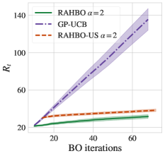
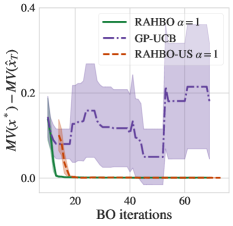
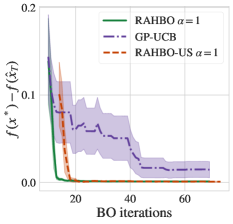
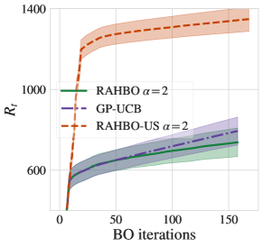
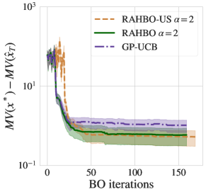
Figure 2: (a) Unknown true objective along with noisy evaluations with varying noise level (left) and unknown true noise variance and its evaluations (right). (b) Cumulative regret. (c) Simple MV regret for reporting rule x^T=argmaxxtlcbT(xt)subscript^𝑥𝑇subscriptargmaxsubscript𝑥𝑡subscriptlcb𝑇subscript𝑥𝑡\hat{x}_{T}=\operatorname*{arg\,max}_{x_{t}}\mathrm{lcb}_{T}(x_{t}). (c) Simple regret f(x)f(x^T)𝑓superscript𝑥𝑓subscript^𝑥𝑇f(x^{*})-f(\hat{x}_{T}) for the unknown function at the reported point x^Tsubscript^𝑥𝑇\hat{x}_{T} from (d). RAHBO not only leads to strong results in terms of MV but also in terms of the mean objective f(x)𝑓𝑥f(x).

Example function We first illustrate the methods performance on a sine function depicted in Figure 2(a). This function has two global optimizers. We induce a heteroscedastic zero-mean Gaussian noise on the measurements. We use a sigmoid function for the noise variance, as depicted in Figure 2(a), that induces small noise on [0,1]01[0,1] and higher noise on (1,2]12(1,2]. We initialize the algorithms by selecting 101010 inputs x𝑥x at random and keep these points the same for all the algorithms. We use k=10𝑘10k=10 samples at each chosen xtsubscript𝑥𝑡x_{t}. The number of acquisition rounds is T=60𝑇60T=60. We repeat the experiment 303030 times for each method and show their average performances in Figure 2.

Refer to caption
Figure 3: GP models fitted for GP-UCB (left) and RAHBO (right) for sine function. After initialization with the same sampled points, GP-UCB concentrates on the high-noise region whereas RAHBO prefers small variance. Additional plots are presented in Section A.6.

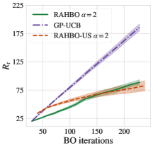
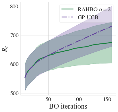
Branin benchmark   Next, we evaluate the methods on the (negated) Branin benchmark function in Figure 1(a), achieving its optimum value f=0.4superscript𝑓0.4f^{*}=-0.4 at (π,12.3),(π,2.3),(9.4,2.5)𝜋12.3𝜋2.39.42.5(-\pi,12.3),(\pi,2.3),(9.4,2.5). The heteroscedastic variance function illustrated in Figure 1(b) defines different noise variances for the three optima. We initialize all algorithms by selecting 101010 inputs. We use k=10𝑘10k=10 samples to estimate the noise variance. The number of acquisition rounds is T=150𝑇150T=150. We repeat BO 252525 times and show the results in Figures 5(a) and 1(c). Figure 1(c) provides more intuition behind the observed regret: UCB exploits the noisiest maxima the most, while RAHBO prefers smaller variance.

Tuning Swiss free-electron laser   In this experiment, we tune the parameters of Swiss X-ray free-electron laser (SwissFEL), an important scientific instrument that generates very short pulses of X-ray light and enables researchers to observe extremely fast processes. The main objective is to maximize the pulse energy measured by a gas detector, that is a time-consuming and repetitive task during the SwissFEL operation. Such (re-)tuning takes place while user experiments on SwissFEL are running, and thus the cumulative regret is the metric of high importance in this application.

We use real SwissFEL measurements collected in [21] to train a neural network surrogate model, and use it to simulate the SwissFEL objective f(x)𝑓𝑥f(x) for new parameter settings x𝑥x. We similarly fit a model of the heteroscedastic variance by regressing the squared residuals via a GP model. Here, we focus on the calibration of the four most sensitive parameters.

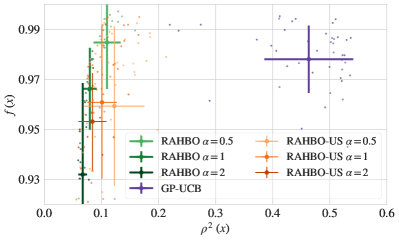
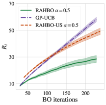
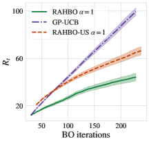
We report our comparison in Figure 4 where we also assess the effect of varying the coefficient of absolute risk tolerance α𝛼\alpha. We use 30 points to initialize the baselines and then perform 200 acquisition rounds. We repeat each experiment 15 times. In Figure 4(a) we plot the empirical frequency of the true (unknown to the methods) values f(xt)𝑓subscript𝑥𝑡f(x_{t}) and ρ2(xt)superscript𝜌2subscript𝑥𝑡\rho^{2}(x_{t}) at the inputs xtsubscript𝑥𝑡x_{t} acquired by the methods. The empirical frequency for ρ2(x)superscript𝜌2𝑥\rho^{2}(x) illustrates the tendency of risk-neutral GP-UCB to query points with higher noise, while risk-averse achieves substantially reduced variance and minimal reduction in mean performance. Sometimes, risk-neutral GP-UCB also fails to succeed in querying points with the highest f𝑓f-value. That tendency results in lower cumulative regret for RAHBO in Figures 4(c) and 4(d). We also compare the performance of the reporting rule from Corollary 1.1 in Figure 4(b), where we plot error bars with standard deviation both for f(x^T)𝑓subscript^𝑥𝑇f(\hat{x}_{T}) and ρ2(x^T)superscript𝜌2subscript^𝑥𝑇\rho^{2}(\hat{x}_{T}) at the reported point x^Tsubscript^𝑥𝑇\hat{x}_{T}. As before, RAHBO drastically reduces the variance compared to GP-UCB, while having only slightly lower mean performance. Additional results are presented in Figure 10 in Appendix.

Refer to caption
(a)
Refer to caption
(b)
Refer to caption
(c)
Refer to caption
(d)
Figure 4: Experimental results for SwissFEL: (a) Distributions of f(x)𝑓𝑥f(x) and ρ2(x)superscript𝜌2𝑥\rho^{2}(x) for all points queried during the optimization. GP-UCB queries points with higher noise (but not necessarily high return f𝑓f) in contrast to the risk-averse methods. (b) Mean f(x^T)𝑓subscript^𝑥𝑇f(\hat{x}_{T}) and variance ρ2(x^T)superscript𝜌2subscript^𝑥𝑇\rho^{2}(\hat{x}_{T}) at the reported x^T=argmaxxtlcbT(xt)subscript^𝑥𝑇subscriptargmaxsubscript𝑥𝑡subscriptlcb𝑇subscript𝑥𝑡\hat{x}_{T}=\operatorname*{arg\,max}_{x_{t}}\mathrm{lcb}_{T}(x_{t}): for each method, we repeat BO experiment 15 times (separate points) and plot corresponding standard deviation error bars. RAHBO reports solutions with reasonable mean-variance tradeoff, while GP-UCB produces solutions with high mean value but also high noise variance. (c-d) Cum. regret for α=0.5𝛼0.5\alpha=0.5 and α=1𝛼1\alpha=1 (see more in Section A.7.1).

Random Forest tuning    BO is widely used by cloud services for tuning machine learning hyperparameters and the resulting models might be then used in high-stakes applications such as credit scoring or fraud detection. In k-fold cross-validation, the average metric over the validation sets is optimized – a canonical example of the repeated experiment setting that we consider in the paper. High across-folds variance is a practical problem [24] where the mean-variance approach might be beneficial.

In our experiment, we tune hyperparameters of a random forest classifier (RF) on a dataset of fraudulent credit card transactions [23].222https://www.kaggle.com/mlg-ulb/creditcardfraud It consist of  285k transactions with 29 features (processed due to confidentiality issues) that are distributed over time, and only 0.2% are fraud examples (see Appendix for more details). The search space for the RF hyperparameters is also provided in the Appendix. We use the balanced accuracy score and 5 validation folds, i.e., k=5𝑘5k=5, and each validation fold is shifted in time with respect to the training data. We seek not only for high performance on average but also for low variance across the validation folds that have different time shifts with respect to the training data.

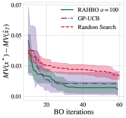
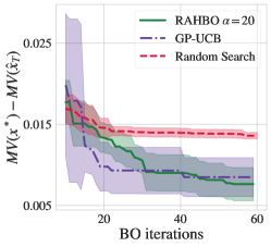
We initialize the algorithms by selecting 10 hyperparameter settings and keep these points the same for all algorithms. We use Matérn 5/2 kernels with Automatic Relevance Discovery (ARD) and normalize the input features to the unit cube. The number of acquisition rounds in one experiment is 50 and we repeat each experiment 15 times. We demonstrate our results in Figures 5(b) and 5(c) where we plot mean ±plus-or-minus\pm 2 standard errors. While both RAHBO and GP-UCB perform comparable in terms of the mean error, its standard deviation for RAHBO is smaller.
Refer to caption
(a)
Refer to caption
(b)
Refer to caption
(c)
Figure 5: Branin: (a) Cumulative regret. Random Forest: (b-c) Simple regret for the reported x^T=argmaxxtMV(xt)subscript^𝑥𝑇subscriptargmaxsubscript𝑥𝑡𝑀𝑉subscript𝑥𝑡\hat{x}_{T}=\operatorname*{arg\,max}_{x_{t}}MV(x_{t}) for (b) α=20𝛼20\alpha=20 and (c) α=100𝛼100\alpha=100. While both methods have comparable mean, RAHBO has consistently lower variance.

5 Conclusion

In this work, we generalize Bayesian optimization to the risk-averse setting and propose RAHBO algorithm aiming to find an input with both large expected return and small input-dependent noise variance. Both the mean objective and the variance are assumed to be unknown a priori and hence are estimated online. RAHBO is equipped with theoretical guarantees showing (under reasonable assumptions) sublinear dependence on the number of evaluation rounds T𝑇T both for cumulative risk-averse regret and ϵitalic-ϵ\epsilon-accurate mean-variance metric. The empirical evaluation of the algorithm on synthetic benchmarks and hyperparameter tuning tasks demonstrate promising examples of heteroscedastic use-cases benefiting from RAHBO.

Acknowledgements

This research has been gratefully supported by NCCR Automation grant 51NF40 180545, by ERC under the European Union’s Horizon grant 815943, SNSF grant 200021_172781, and ETH Zürich Postdoctoral Fellowship 19-2 FEL-47. The authors thank Sebastian Curi, Mojmír Mutný and Johannes Kirschner as well as the anonymous reviewers of this paper for their helpful feedback.

References

  • [1] Y. Abbasi-Yadkori. Online learning for linearly parametrized control problems. PhD thesis, Edmonton, Alberta, 2012.
  • [2] J. Arbel, O. Marchal, and H. D. Nguyen. On strict sub-Gaussianity, optimal proxy variance and symmetry for bounded random variables. arXiv:1901.09188, 2019.
  • [3] M. Balandat, B. Karrer, D. R. Jiang, S. Daulton, B. Letham, A. G. Wilson, and E. Bakshy. BoTorch: a framework for efficient Monte-Carlo Bayesian optimization. In Neural Information Processing Systems (NeurIPS), 2020.
  • [4] E. Benhamou. A few properties of sample variance. arXiv:1809.03774, 2018.
  • [5] F. Berkenkamp, A. Krause, and A. P. Schoellig. Bayesian optimization with safety constraints: Safe and automatic parameter tuning in robotics. arXiv:1602.04450, 2016.
  • [6] M. Binois, R. B. Gramacy, and M. Ludkovski. Practical heteroscedastic Gaussian process modeling for large simulation experiments. Journal of Computational and Graphical Statistics, 2018.
  • [7] M. Binois, J. Huang, R. B. Gramacy, and M. Ludkovski. Replication or exploration: Sequential design for stochastic simulation experiments. In Technometrics, 2019.
  • [8] I. Bogunovic, A. Krause, and J. Scarlett. Corruption-tolerant Gaussian process bandit optimization. In Conference on Artificial Intelligence and Statistics (AISTATS), 2020.
  • [9] I. Bogunovic, J. Scarlett, S. Jegelka, and V. Cevher. Adversarially robust optimization with Gaussian processes. In Neural Information Processing Systems (NeurIPS), 2018.
  • [10] I. Bogunovic, J. Scarlett, A. Krause, and V. Cevher. Truncated variance reduction: A unified approach to Bayesian optimization and level-set estimation. In Neural Information Processing Systems (NeurIPS), 2016.
  • [11] S. Cakmak, R. Astudillo, P. I. Frazier, and E. Zhou. Bayesian optimization of risk measures. In Neural Information Processing Systems (NeurIPS), 2020.
  • [12] R. Calandra, A. Seyfarth, J. Peters, and M. P. Deisenroth. Bayesian optimization for learning gaits under uncertainty. Annals of Mathematics and Artificial Intelligence, 2016.
  • [13] Y. Chen, A. Huang, Z. Wang, I. Antonoglou, J. Schrittwieser, D. Silver, and N. de Freitas. Bayesian optimization in Alphago. arXiv:1812.06855, 2018.
  • [14] S. R. Chowdhury and A. Gopalan. On kernelized multi-armed bandits. In International Conference on Machine Learning (ICML), 2017.
  • [15] A. I. Cowen-Rivers, W. Lyu, R. Tutunov, Z. Wang, A. Grosnit, R. R. Griffiths, H. Jianye, J. Wang, and H. B. Ammar. An empirical study of assumptions in Bayesian optimisation. arXiv:2012.03826, 2021.
  • [16] J. González, J. Longworth, D. C. James, and N. D. Lawrence. Bayesian optimization for synthetic gene design. arXiv:1505.01627, 2015.
  • [17] R.-R. Griffiths and J. M. Hernández-Lobato. Constrained Bayesian optimization for automatic chemical design using variational autoencoders. Chemical Science, 2020.
  • [18] S. Iwazaki, Y. Inatsu, and I. Takeuchi. Mean-variance analysis in Bayesian optimization under uncertainty. In Conference on Artificial Intelligence and Statistics (AISTATS), 2021.
  • [19] J. Kirschner, I. Bogunovic, S. Jegelka, and A. Krause. Distributionally robust Bayesian optimization. In Conference on Artificial Intelligence and Statistics (AISTATS), 2020.
  • [20] J. Kirschner and A. Krause. Information directed sampling and bandits with heteroscedastic noise. In Conference On Learning Theory (COLT), 2018.
  • [21] J. Kirschner, M. Mutny, N. Hiller, R. Ischebeck, and A. Krause. Adaptive and safe Bayesian optimization in high dimensions via one-dimensional subspaces. In International Conference on Machine Learning (ICML), 2019.
  • [22] K. Korovina, S. Xu, K. Kandasamy, W. Neiswanger, B. Poczos, J. Schneider, and E. P. Xing. Chembo: Bayesian optimization of small organic molecules with synthesizable recommendations. arXiv:1908.01425, 2019.
  • [23] Y.-A. Le Borgne and G. Bontempi. Machine Learning for Credit Card Fraud Detection - Practical Handbook. Université Libre de Bruxelles, 2021.
  • [24] A. Makarova, H. Shen, V. Perrone, A. Klein, J. B. Faddoul, A. Krause, M. Seeger, and C. Archambeau. Overfitting in Bayesian optimization: an empirical study and early-stopping solution. In ICLR Workshop on Neural Architecture Search, 2021.
  • [25] A. Marco, P. Hennig, J. Bohg, S. Schaal, and S. Trimpe. Automatic LQR tuning based on Gaussian process global optimization. In International Conference on Robotics and Automation (ICRA), 2016.
  • [26] J. Močkus. On Bayesian methods for seeking the extremum. In Optimization Techniques, 1975.
  • [27] H. Moss, D. Leslie, D. Beck, J. González, and P. Rayson. BOSS: Bayesian optimization over string spaces. In Neural Information Processing Systems (NeurIPS), 2020.
  • [28] D. M. Negoescu, P. I. Frazier, and W. B. Powell. The knowledge-gradient algorithm for sequencing experiments in drug discovery. INFORMS J. on Computing, 2011.
  • [29] Q. P. Nguyen, Z. Dai, B. K. H. Low, and P. Jaillet. Value-at-risk optimization with Gaussian processes. In International Conference on Machine Learning (ICML), 2021.
  • [30] T. Nguyen, S. Gupta, H. Ha, S. Rana, and S. Venkatesh. Distributionally robust Bayesian quadrature optimization. In Conference on Artificial Intelligence and Statistics (AISTATS), 2020.
  • [31] S. Ray Chowdhury and A. Gopalan. Bayesian optimization under heavy-tailed payoffs. In Neural Information Processing Systems (NeurIPS), 2019.
  • [32] A. Sani, A. Lazaric, and R. Munos. Risk-aversion in multi-armed bandits. In Neural Information Processing Systems (NeurIPS), 2012.
  • [33] P. G. Sessa, I. Bogunovic, M. Kamgarpour, and A. Krause. Mixed strategies for robust optimization of unknown objectives. In Conference on Artificial Intelligence and Statistics (AISTATS), 2020.
  • [34] J. Snoek, H. Larochelle, and R. P. Adams. Practical Bayesian optimization of machine learning algorithms. In Neural Information Processing Systems (NeurIPS), 2012.
  • [35] N. Srinivas, A. Krause, S. Kakade, and M. Seeger. Gaussian process optimization in the bandit setting: No regret and experimental design. In International Conference on International Conference on Machine Learning (ICML), 2010.

Appendix A Appendix
Risk-averse Heteroscedastic Bayesian Optimization
(Anastasiia Makarova, Ilnura Usmanova, Ilija Bogunovic, Andreas Krause)

A.1 Details on Proposition 1

We first provide the proof of Proposition 1 for cumulative risk-averse regret Eq. 3 with known variance-proxy ρ2()superscript𝜌2\rho^{2}(\cdot) (see Definition 1) (Section A.1.1). We further provide data-independent bounds for βTsubscript𝛽𝑇\beta_{T} (Section A.1.2) and maximum information gain γTsubscript𝛾𝑇\gamma_{T} (Section A.1.3) that together conclude the proof for sub-linear on T𝑇T regret guarantees for most of the popularly used kernels.

A.1.1 Proof Proposition 1

Proposition 1. Consider any fκ𝑓subscript𝜅f\in\mathcal{H}_{\kappa} with fκfsubscriptnorm𝑓𝜅subscript𝑓\|f\|_{\kappa}\leq\mathcal{B}_{f} and sampling model from Eq. 1 with known variance-proxy ρ2(x)superscript𝜌2𝑥\rho^{2}(x). Let {βt}t=1Tsuperscriptsubscriptsubscript𝛽𝑡𝑡1𝑇\{\beta_{t}\}_{t=1}^{T} be set as in Lemma 1 with λ=1𝜆1\lambda=1. Then, with probability at least 1δ1𝛿1-\delta, RAHBO attains cumulative risk-averse regret RT=𝒪(βTTγT(ϱ¯2+1))subscript𝑅𝑇𝒪subscript𝛽𝑇𝑇subscript𝛾𝑇superscript¯italic-ϱ21R_{T}=\mathcal{O}\big{(}\beta_{T}\sqrt{T\gamma_{T}(\bar{\varrho}^{2}+1)}\big{)}.

Proof.

The main steps of the proof are as follows: In Step 1, we derive the upper and the lower confidence bounds, ucbtMV(xt)subscriptsuperscriptucbMV𝑡subscript𝑥𝑡\mathrm{ucb}^{\text{MV}}_{t}(x_{t}) and lcbtMV(xt)subscriptsuperscriptlcbMV𝑡subscript𝑥𝑡\mathrm{lcb}^{\text{MV}}_{t}(x_{t}), on MV(xt)MVsubscript𝑥𝑡\text{MV}(x_{t}) at iteration t𝑡t. In Step 2, we bound the instantaneous risk-averse regret r(xt):=MV(x)MV(xt)assign𝑟subscript𝑥𝑡MVsuperscript𝑥MVsubscript𝑥𝑡r(x_{t}):=\text{MV}(x^{*})-\text{MV}(x_{t}). In Step 3, we derive mutual information I(y1:T,f1:T)𝐼subscript𝑦:1𝑇subscript𝑓:1𝑇I(y_{1:T},f_{1:T}) in case of the heteroscedastic noise. In Step 4, we bound the sum of variances t=1Tσt1(xt)superscriptsubscript𝑡1𝑇subscript𝜎𝑡1subscript𝑥𝑡\sum_{t=1}^{T}\sigma_{t-1}(x_{t}) via mutual information I(y1:T,f1:T)𝐼subscript𝑦:1𝑇subscript𝑓:1𝑇I(y_{1:T},f_{1:T}). In Step 5, we bound the cumulative regret RT=t=1Tr(xt)subscript𝑅𝑇superscriptsubscript𝑡1𝑇𝑟subscript𝑥𝑡R_{T}=\sum_{t=1}^{T}r(x_{t}) based on the previous steps.

Step 1: On the confidence bounds for MV(x)MV𝑥\text{MV}(x).
In case of known variance-proxy ρ2(x)superscript𝜌2𝑥\rho^{2}(x), the confidence bounds for MV(x)MV𝑥\text{MV}(x) at iteration t𝑡t can be directly obtained based on the posterior μt(x)subscript𝜇𝑡𝑥\mu_{t}(x) and σt(x)subscript𝜎𝑡𝑥\sigma_{t}(x) for f(x)𝑓𝑥f(x) defined in Eqs. 5 and 6. Particularly, for βt=βt(δ)subscript𝛽𝑡subscript𝛽𝑡𝛿\beta_{t}=\beta_{t}(\delta) defined in Eq. 8, Pr{lcbtMV(x)MV(x)ucbtMV(x)x𝒳,t0}1δPrsuperscriptsubscriptlcb𝑡MV𝑥MV𝑥superscriptsubscriptucb𝑡MV𝑥for-all𝑥𝒳for-all𝑡01𝛿\Pr\big{\{}\mathrm{lcb}_{t}^{\text{MV}}(x)\leq\text{MV}(x)\leq\mathrm{ucb}_{t}^{\text{MV}}(x)~{}\forall x\in\mathcal{X},\forall t\geq 0\big{\}}\geq 1-\delta with the confidence bounds:

lcbtMV(x):=μt1(x)βtσt1(x)αρ2(x),assignsubscriptsuperscriptlcbMV𝑡𝑥subscript𝜇𝑡1𝑥subscript𝛽𝑡subscript𝜎𝑡1𝑥𝛼superscript𝜌2𝑥\displaystyle\mathrm{lcb}^{\text{MV}}_{t}(x):=\mu_{t-1}(x)-\beta_{t}\sigma_{t-1}(x)-\alpha\rho^{2}(x), (18)
ucbtMV(x):=μt1(x)+βtσt1(x)αρ2(x).assignsubscriptsuperscriptucbMV𝑡𝑥subscript𝜇𝑡1𝑥subscript𝛽𝑡subscript𝜎𝑡1𝑥𝛼superscript𝜌2𝑥\displaystyle\mathrm{ucb}^{\text{MV}}_{t}(x):=\mu_{t-1}(x)+\beta_{t}\sigma_{t-1}(x)-\alpha\rho^{2}(x). (19)

Step 2: On bounding the instantaneous risk-averse regret rt(x)subscript𝑟𝑡𝑥r_{t}(x). We have

r(xt)𝑟subscript𝑥𝑡\displaystyle r(x_{t}) =MV(x)MV(xt)absentMVsuperscript𝑥MVsubscript𝑥𝑡\displaystyle={\text{MV}}(x^{*})-{\text{MV}}(x_{t})
ucbtMV(x)lcbtMV(xt)absentsubscriptsuperscriptucbMV𝑡superscript𝑥subscriptsuperscriptlcbMV𝑡subscript𝑥𝑡\displaystyle\leq\mathrm{ucb}^{\text{MV}}_{t}(x^{*})-\mathrm{lcb}^{\text{MV}}_{t}(x_{t})
ucbtMV(xt)lcbtMV(xt)=2βtσt1(xt),absentsubscriptsuperscriptucbMV𝑡subscript𝑥𝑡subscriptsuperscriptlcbMV𝑡subscript𝑥𝑡2subscript𝛽𝑡subscript𝜎𝑡1subscript𝑥𝑡\displaystyle\leq\mathrm{ucb}^{\text{MV}}_{t}(x_{t})-\mathrm{lcb}^{\text{MV}}_{t}(x_{t})=2\beta_{t}\sigma_{t-1}(x_{t}),

where the first inequality is due to the definition of confidence bounds, the second is due to the acquisition strategy xtargmaxx𝒳ucbtMV(x);subscript𝑥𝑡subscriptargmax𝑥𝒳subscriptsuperscriptucbMV𝑡𝑥x_{t}\in\operatorname*{arg\,max}_{x\in\mathcal{X}}\mathrm{ucb}^{\text{MV}}_{t}(x); and the equality further expands lcbtMV(x)subscriptsuperscriptlcbMV𝑡𝑥\mathrm{lcb}^{\text{MV}}_{t}(x) and ucbtMV(x).subscriptsuperscriptucbMV𝑡𝑥\mathrm{ucb}^{\text{MV}}_{t}(x). Thus, the cumulative regret can be bounded as follows:

RT=t=1Tr(xt)t=1T2βtσt1(xt)2βTt=1Tσt1(xt),subscript𝑅𝑇superscriptsubscript𝑡1𝑇𝑟subscript𝑥𝑡superscriptsubscript𝑡1𝑇2subscript𝛽𝑡subscript𝜎𝑡1subscript𝑥𝑡2subscript𝛽𝑇superscriptsubscript𝑡1𝑇subscript𝜎𝑡1subscript𝑥𝑡\displaystyle R_{T}=\sum_{t=1}^{T}r(x_{t})\leq\sum_{t=1}^{T}2\beta_{t}\sigma_{t-1}(x_{t})\leq 2\beta_{T}\sum_{t=1}^{T}\sigma_{t-1}(x_{t}), (20)

where the last inequality holds since {βt}t=1Tsuperscriptsubscriptsubscript𝛽𝑡𝑡1𝑇\{\beta_{t}\}_{t=1}^{T} is a non-decreasing sequence.

Step 3: On mutual information I(y1:T,f1:T)𝐼subscript𝑦:1𝑇subscript𝑓:1𝑇I(y_{1:T},f_{1:T}) and maximum information gain γTsubscript𝛾𝑇\gamma_{T}.
Mutual information I(y1:T,f1:T)𝐼subscript𝑦:1𝑇subscript𝑓:1𝑇I(y_{1:T},f_{1:T}) between the vector of evaluations y1:TTsubscript𝑦:1𝑇superscript𝑇y_{1:T}\in\mathbb{R}^{T} at points A={xt}t=1T𝐴superscriptsubscriptsubscript𝑥𝑡𝑡1𝑇A=\{x_{t}\}_{t=1}^{T} and f1:T=[f(x1),,f(xT)]subscript𝑓:1𝑇superscript𝑓subscript𝑥1𝑓subscript𝑥𝑇topf_{1:T}=[f(x_{1}),\dots,f(x_{T})]^{\top} is defined by

I(y1:T,f1:T)=H(y1:T)H(y1:T|f1:T),𝐼subscript𝑦:1𝑇subscript𝑓:1𝑇𝐻subscript𝑦:1𝑇𝐻conditionalsubscript𝑦:1𝑇subscript𝑓:1𝑇I(y_{1:T},f_{1:T})=H(y_{1:T})-H(y_{1:T}|f_{1:T}),

where H()𝐻H(\cdot) denotes entropy. Under the modelling assumptions f1:T𝒩(0,λ1KT)similar-tosubscript𝑓:1𝑇𝒩0superscript𝜆1subscript𝐾𝑇f_{1:T}\sim\mathcal{N}(0,\lambda^{-1}K_{T}) and ξ1:T𝒩(0,ΣT)similar-tosubscript𝜉:1𝑇𝒩0subscriptΣ𝑇\xi_{1:T}\sim\mathcal{N}(0,\Sigma_{T}) for the noise ξ1:T=[ξ(x1),,ξ(xT)]subscript𝜉:1𝑇superscript𝜉subscript𝑥1𝜉subscript𝑥𝑇top\xi_{1:T}=[\xi(x_{1}),\dots,\xi(x_{T})]^{\top}, the measurements are distributed as y1:T𝒩(0,λ1KT+ΣT)similar-tosubscript𝑦:1𝑇𝒩0superscript𝜆1subscript𝐾𝑇subscriptΣ𝑇y_{1:T}\sim\mathcal{N}(0,\lambda^{-1}K_{T}+\Sigma_{T}) and yt|y1:t1𝒩(μt1(xt),ρ2(xt)+σt12(xt))similar-toconditionalsubscript𝑦𝑡subscript𝑦:1𝑡1𝒩subscript𝜇𝑡1subscript𝑥𝑡superscript𝜌2subscript𝑥𝑡subscriptsuperscript𝜎2𝑡1subscript𝑥𝑡y_{t}|y_{1:t-1}\sim\mathcal{N}(\mu_{t-1}(x_{t}),\rho^{2}(x_{t})+\sigma^{2}_{t-1}(x_{t})), where σt12()subscriptsuperscript𝜎2𝑡1\sigma^{2}_{t-1}(\cdot) is defined in Eq. 6. Hence, the entropy of each new measurement ytsubscript𝑦𝑡y_{t} conditioned on the previous history y1:t1subscript𝑦:1𝑡1y_{1:t-1} is:

H(yt|y1:t1)𝐻conditionalsubscript𝑦𝑡subscript𝑦:1𝑡1\displaystyle H(y_{t}|y_{1:t-1}) =12ln(2πe(ρ2(xt)+σt12(xt)))absent122𝜋𝑒superscript𝜌2subscript𝑥𝑡subscriptsuperscript𝜎2𝑡1subscript𝑥𝑡\displaystyle=\frac{1}{2}\ln\left(2\pi e\left(\rho^{2}(x_{t})+\sigma^{2}_{t-1}(x_{t})\right)\right)
=12ln(2πeρ2(xt)(1+σt12(xt)ρ2(xt)))absent122𝜋𝑒superscript𝜌2subscript𝑥𝑡1subscriptsuperscript𝜎2𝑡1subscript𝑥𝑡superscript𝜌2subscript𝑥𝑡\displaystyle=\frac{1}{2}\ln\bigg{(}2\pi e\rho^{2}(x_{t})\left(1+\frac{\sigma^{2}_{t-1}(x_{t})}{\rho^{2}(x_{t})}\right)\bigg{)}
=12ln(2πeρ2(xt))+12ln(1+σt12(xt)ρ2(xt)),absent122𝜋𝑒superscript𝜌2subscript𝑥𝑡121subscriptsuperscript𝜎2𝑡1subscript𝑥𝑡superscript𝜌2subscript𝑥𝑡\displaystyle=\frac{1}{2}\ln\bigg{(}2\pi e\rho^{2}(x_{t})\bigg{)}+\frac{1}{2}\ln\bigg{(}1+\frac{\sigma^{2}_{t-1}(x_{t})}{\rho^{2}(x_{t})}\bigg{)},
H(y1:T)𝐻subscript𝑦:1𝑇\displaystyle H(y_{1:T}) =t=1TH(yt|y1:t1)=12t=1Tln(2πeρ2(xt))+12t=1Tln(1+σt12(xt)ρ2(xt)),absentsuperscriptsubscript𝑡1𝑇𝐻conditionalsubscript𝑦𝑡subscript𝑦:1𝑡112superscriptsubscript𝑡1𝑇2𝜋𝑒superscript𝜌2subscript𝑥𝑡12superscriptsubscript𝑡1𝑇1subscriptsuperscript𝜎2𝑡1subscript𝑥𝑡superscript𝜌2subscript𝑥𝑡\displaystyle=\sum_{t=1}^{T}H(y_{t}|y_{1:t-1})=\frac{1}{2}\sum_{t=1}^{T}\ln\bigg{(}2\pi e\rho^{2}(x_{t})\bigg{)}+\frac{1}{2}\sum_{t=1}^{T}\ln\bigg{(}1+\frac{\sigma^{2}_{t-1}(x_{t})}{\rho^{2}(x_{t})}\bigg{)},
H(y1:T|f1:T)𝐻conditionalsubscript𝑦:1𝑇subscript𝑓:1𝑇\displaystyle H(y_{1:T}|f_{1:T}) =t=1TH(yt|ft)=12t=1Tln(2πeρ2(xt)).absentsuperscriptsubscript𝑡1𝑇𝐻conditionalsubscript𝑦𝑡subscript𝑓𝑡12superscriptsubscript𝑡1𝑇2𝜋𝑒superscript𝜌2subscript𝑥𝑡\displaystyle=\sum_{t=1}^{T}H(y_{t}|f_{t})=\frac{1}{2}\sum_{t=1}^{T}\ln(2\pi e\rho^{2}(x_{t})).

Therefore, the information gain for y1:Tsubscript𝑦:1𝑇y_{1:T} is:

I(y1:T,f1:T)=H(y1:T)H(y1:T|f1:T)=12t=1Tln(1+σt12(xt)ρ2(xt)).𝐼subscript𝑦:1𝑇subscript𝑓:1𝑇𝐻subscript𝑦:1𝑇𝐻conditionalsubscript𝑦:1𝑇subscript𝑓:1𝑇12superscriptsubscript𝑡1𝑇1subscriptsuperscript𝜎2𝑡1subscript𝑥𝑡superscript𝜌2subscript𝑥𝑡\displaystyle I(y_{1:T},f_{1:T})=H(y_{1:T})-H(y_{1:T}|f_{1:T})=\frac{1}{2}\sum_{t=1}^{T}\ln\bigg{(}1+\frac{\sigma^{2}_{t-1}(x_{t})}{\rho^{2}(x_{t})}\bigg{)}. (21)

Then, by definition of maximum information gain:

γT:=maxA𝒳,|A|=TI(y1:T,f1:T)12t=1Tln(1+σt12(xt)ρ2(xt)).assignsubscript𝛾𝑇formulae-sequence𝐴𝒳𝐴𝑇𝐼subscript𝑦:1𝑇subscript𝑓:1𝑇12superscriptsubscript𝑡1𝑇1subscriptsuperscript𝜎2𝑡1subscript𝑥𝑡superscript𝜌2subscript𝑥𝑡\displaystyle\gamma_{T}:=\underset{A\subset\mathcal{X},\;|A|=T}{\max}\;I(y_{1:T},f_{1:T})\geq\frac{1}{2}\sum_{t=1}^{T}\ln\bigg{(}1+\frac{\sigma^{2}_{t-1}(x_{t})}{\rho^{2}(x_{t})}\bigg{)}. (22)

Step 4: On bounding t=1Tσt1(xt)superscriptsubscript𝑡1𝑇subscript𝜎𝑡1subscript𝑥𝑡\sum_{t=1}^{T}\sigma_{t-1}(x_{t}).

t=1Tσt1(xt)superscriptsubscript𝑡1𝑇subscript𝜎𝑡1subscript𝑥𝑡\displaystyle\sum_{t=1}^{T}\sigma_{t-1}(x_{t}) =t=1Tρ(xt)ρ(xt)σt1(xt)Tt=1Tρ2(xt)σt12(xt)ρ2(xt)absentsuperscriptsubscript𝑡1𝑇𝜌subscript𝑥𝑡𝜌subscript𝑥𝑡subscript𝜎𝑡1subscript𝑥𝑡𝑇superscriptsubscript𝑡1𝑇superscript𝜌2subscript𝑥𝑡subscriptsuperscript𝜎2𝑡1subscript𝑥𝑡superscript𝜌2subscript𝑥𝑡\displaystyle=\sum_{t=1}^{T}\frac{\rho(x_{t})}{\rho(x_{t})}\sigma_{t-1}(x_{t})\leq\sqrt{T\sum_{t=1}^{T}\rho^{2}(x_{t})\frac{\sigma^{2}_{t-1}(x_{t})}{\rho^{2}(x_{t})}}
Tt=1T1ln(1+ρ2(xt))ln(1+σt12(xt)ρ2(xt))absent𝑇superscriptsubscript𝑡1𝑇11superscript𝜌2subscript𝑥𝑡1superscriptsubscript𝜎𝑡12subscript𝑥𝑡superscript𝜌2subscript𝑥𝑡\displaystyle\leq\sqrt{T\sum_{t=1}^{T}\frac{1}{\ln(1+\rho^{-2}(x_{t}))}\ln\bigg{(}1+\frac{\sigma_{t-1}^{2}(x_{t})}{\rho^{2}(x_{t})}\bigg{)}}
2Tln(1+ϱ¯2)12t=1Tln(1+σt12(xt)ρ2(xt))mutualinformationEq. 21,absent2𝑇1superscript¯italic-ϱ2subscript12superscriptsubscript𝑡1𝑇1superscriptsubscript𝜎𝑡12subscript𝑥𝑡superscript𝜌2subscript𝑥𝑡mutualinformationEq. 21\displaystyle\leq\sqrt{\frac{2T}{\ln(1+\bar{\varrho}^{-2})}\underbrace{\frac{1}{2}\sum_{t=1}^{T}\ln\bigg{(}1+\frac{\sigma_{t-1}^{2}(x_{t})}{\rho^{2}(x_{t})}\bigg{)}}_{\mathrm{mutual~{}information~{}\lx@cref{creftype~refnum}{app:eq_information_gain_known_rho}}}}, (23)

where the first inequality follows from the Cauchy-Schwarz inequality. The second one is due to the fact that for any s2[0,ρ2(xt)]superscript𝑠20superscript𝜌2subscript𝑥𝑡s^{2}\in[0,\rho^{-2}(x_{t})] we can bound s2ρ2(xt)ln(1+ρ2(xt))ln(1+s2)superscript𝑠2superscript𝜌2subscript𝑥𝑡1superscript𝜌2subscript𝑥𝑡1superscript𝑠2s^{2}\leq\frac{\rho^{-2}(x_{t})}{\ln(1+\rho^{-2}(x_{t}))}\ln(1+s^{2}), that also holds for s2:=ρ2(xt)σt12(xt)assignsuperscript𝑠2superscript𝜌2subscript𝑥𝑡subscriptsuperscript𝜎2𝑡1subscript𝑥𝑡s^{2}:=\rho^{-2}(x_{t})\sigma^{2}_{t-1}(x_{t}) since ρ2(xt)σt12(xt)ρ2(xt)λ1κ(xt,xt)ρ2(xt)superscript𝜌2subscript𝑥𝑡subscriptsuperscript𝜎2𝑡1subscript𝑥𝑡superscript𝜌2subscript𝑥𝑡superscript𝜆1𝜅subscript𝑥𝑡subscript𝑥𝑡superscript𝜌2subscript𝑥𝑡\rho^{-2}(x_{t})\sigma^{2}_{t-1}(x_{t})\leq\rho^{-2}(x_{t})\lambda^{-1}\kappa(x_{t},x_{t})\leq\rho^{-2}(x_{t}) for λ1𝜆1\lambda\geq 1. The third inequality is due to ρ(x)[ϱ¯,ϱ¯]𝜌𝑥¯italic-ϱ¯italic-ϱ\rho(x)\in[\smash{\underline{\varrho}},\bar{\varrho}].

Step 5: Bounding risk-averse cumulative regret RT=t=1Tr(xt)subscript𝑅𝑇superscriptsubscript𝑡1𝑇𝑟subscript𝑥𝑡R_{T}=\sum_{t=1}^{T}r(x_{t}).
Combining the previous three steps together: Eq. 20, Eq. 22, and Eq. 23 we finally obtain:

RTt=1T2βtσt1(xt)2βTt=1Tσt1(xt)2βT2Tln(1+ϱ¯2)γTsubscript𝑅𝑇superscriptsubscript𝑡1𝑇2subscript𝛽𝑡subscript𝜎𝑡1subscript𝑥𝑡2subscript𝛽𝑇superscriptsubscript𝑡1𝑇subscript𝜎𝑡1subscript𝑥𝑡2subscript𝛽𝑇2𝑇1superscript¯italic-ϱ2subscript𝛾𝑇\displaystyle R_{T}\leq\sum_{t=1}^{T}2\beta_{t}\sigma_{t-1}(x_{t})\leq 2\beta_{T}\sum_{t=1}^{T}\sigma_{t-1}(x_{t})\leq 2\beta_{T}\sqrt{\frac{2T}{\ln(1+\bar{\varrho}^{-2})}\gamma_{T}}

Also, note that for any α0𝛼0\alpha\geq 0 the bound ln(1+α)α1+α1𝛼𝛼1𝛼\ln(1+\alpha)\geq\frac{\alpha}{1+\alpha} holds, thus 1ln(1+ϱ¯2)1+ϱ¯2ϱ¯2=ϱ¯2+1.11superscript¯italic-ϱ21superscript¯italic-ϱ2superscript¯italic-ϱ2superscript¯italic-ϱ21\frac{1}{\ln(1+\bar{\varrho}^{-2})}\leq\frac{1+\bar{\varrho}^{-2}}{\bar{\varrho}^{-2}}=\bar{\varrho}^{2}+1. Therefore, the cumulative regret can be also bounded as RT=O(βTTγT(ϱ¯2+1)).subscript𝑅𝑇𝑂subscript𝛽𝑇𝑇subscript𝛾𝑇superscript¯italic-ϱ21R_{T}=O(\beta_{T}\sqrt{T\gamma_{T}(\bar{\varrho}^{2}+1)}).

A.1.2 Bounds for βTsubscript𝛽𝑇\beta_{T}

We provide the bounds for the data-dependent βTsubscript𝛽𝑇\beta_{T} that appear in the regret bound (see Eq. 8). Following our modelling assumptions f1:T𝒩(0,λ1KT)similar-tosubscript𝑓:1𝑇𝒩0superscript𝜆1subscript𝐾𝑇f_{1:T}\sim\mathcal{N}(0,\lambda^{-1}K_{T}) and ξ1:T𝒩(0,ΣT)similar-tosubscript𝜉:1𝑇𝒩0subscriptΣ𝑇\xi_{1:T}\sim\mathcal{N}(0,\Sigma_{T}), the information gain I(y1:T,f1:T)=H(y1:T)H(y1:T|f1:T)𝐼subscript𝑦:1𝑇subscript𝑓:1𝑇𝐻subscript𝑦:1𝑇𝐻conditionalsubscript𝑦:1𝑇subscript𝑓:1𝑇I(y_{1:T},f_{1:T})=H(y_{1:T})-H(y_{1:T}|f_{1:T}) is given as follows:

I(y1:T,f1:T)=12ln(det(2πe(λ1KT+ΣT)))H(y1:T)12ln(det(2πeΣT))H(y1:T|f1:T)=12ln(det(KT+λΣT)det(λΣT)).𝐼subscript𝑦:1𝑇subscript𝑓:1𝑇subscript122𝜋𝑒superscript𝜆1subscript𝐾𝑇subscriptΣ𝑇𝐻subscript𝑦:1𝑇subscript122𝜋𝑒subscriptΣ𝑇𝐻conditionalsubscript𝑦:1𝑇subscript𝑓:1𝑇12subscript𝐾𝑇𝜆subscriptΣ𝑇𝜆subscriptΣ𝑇\displaystyle I(y_{1:T},f_{1:T})=\underbrace{\frac{1}{2}\ln\big{(}\det(2\pi e(\lambda^{-1}K_{T}+\Sigma_{T}))\big{)}}_{H(y_{1:T})}-\underbrace{\frac{1}{2}\ln\big{(}\det(2\pi e\Sigma_{T})\big{)}}_{H(y_{1:T}|f_{1:T})}=\frac{1}{2}\ln\left(\frac{\det(K_{T}+\lambda\Sigma_{T})}{\det(\lambda\Sigma_{T})}\right). (24)

By definition then γT=maxA𝒳,|A|=TI(y1:T,f1:T)12ln(det(KT+λΣT)det(λΣT))subscript𝛾𝑇formulae-sequence𝐴𝒳𝐴𝑇𝐼subscript𝑦:1𝑇subscript𝑓:1𝑇12subscript𝐾𝑇𝜆subscriptΣ𝑇𝜆subscriptΣ𝑇\gamma_{T}=\underset{A\subset\mathcal{X},\;|A|=T}{\max}\;I(y_{1:T},f_{1:T})\geq\frac{1}{2}\ln\left(\frac{\det(K_{T}+\lambda\Sigma_{T})}{\det(\lambda\Sigma_{T})}\right). On the other hand, βTsubscript𝛽𝑇\beta_{T} defined in Lemma 1 can be expanded in a data-independent manner as follows:

βTsubscript𝛽𝑇\displaystyle\beta_{T} :=2ln(det(λΣT+KT)1/2δdet(λΣT)1/2)+λfκ\displaystyle:=\sqrt{2\ln\bigg{(}\frac{\det(\lambda\Sigma_{T}+K_{T})^{1/2}}{\delta\det(\lambda\Sigma_{T})^{1/2}}}\bigg{)}+\sqrt{\lambda}\|f\|_{\kappa}
=2ln1δ+ln(det(λΣT+KT)det(λΣT))+λfκ2ln1δ+γT+λBf.absent21𝛿𝜆subscriptΣ𝑇subscript𝐾𝑇𝜆subscriptΣ𝑇𝜆subscriptnorm𝑓𝜅21𝛿subscript𝛾𝑇𝜆subscript𝐵𝑓\displaystyle=\sqrt{2\ln\frac{1}{\delta}+\ln\left(\frac{\det(\lambda\Sigma_{T}+K_{T})}{\det(\lambda\Sigma_{T})}\right)}+\sqrt{\lambda}\|f\|_{\kappa}\leq\sqrt{2\ln\frac{1}{\delta}+\gamma_{T}}+\sqrt{\lambda}B_{f}. (25)

A.1.3 Bounds for γTsubscript𝛾𝑇\gamma_{T}

Here, we show the relation between the information gains under heteroscedastic and homoscedastic noise. Note that for the latter the upper bounds are widely known, e.g., [35]. To distinguish between the maximum information gain for heteroscedastic noise with variance-proxy ρ2(x)superscript𝜌2𝑥\rho^{2}(x) and the maximum information gain for homoscedastic noise with fixed variance-proxy σ2superscript𝜎2\sigma^{2}, we denote them as γTρxsuperscriptsubscript𝛾𝑇subscript𝜌𝑥\gamma_{T}^{\rho_{x}} and γTσsuperscriptsubscript𝛾𝑇𝜎\gamma_{T}^{\sigma} respectively. Recall that ϱ2()[ϱ¯2,ϱ¯2]superscriptitalic-ϱ2superscript¯italic-ϱ2superscript¯italic-ϱ2\varrho^{2}(\cdot)\in[\smash{\underline{\varrho}^{2}},\bar{\varrho}^{2}] for some constant values ϱ¯2ϱ¯2>0superscript¯italic-ϱ2superscript¯italic-ϱ20\bar{\varrho}^{2}\geq\smash{\underline{\varrho}^{2}}>0.

Below, we show that γTρxγTσϱ¯2ϱ¯2superscriptsubscript𝛾𝑇subscript𝜌𝑥superscriptsubscript𝛾𝑇𝜎superscript¯italic-ϱ2superscript¯italic-ϱ2\gamma_{T}^{\rho_{x}}\leq\gamma_{T}^{\sigma}\frac{\bar{\varrho}^{2}}{\smash{\underline{\varrho}^{2}}} with σ2superscript𝜎2\sigma^{2} set to ϱ¯2superscript¯italic-ϱ2\bar{\varrho}^{2}, that only affects the constants but not the main scaling (in terms of T𝑇T) of the known bound for the homoscedastic maximum information gain.

γTρxsuperscriptsubscript𝛾𝑇subscript𝜌𝑥\displaystyle\gamma_{T}^{\rho_{x}} =1maxA𝒳,|A|=T12t=1Tln(1+σt12(xt|ρ2(xt))ρ2(xt))1formulae-sequence𝐴𝒳𝐴𝑇12superscriptsubscript𝑡1𝑇1subscriptsuperscript𝜎2𝑡1conditionalsubscript𝑥𝑡superscript𝜌2subscript𝑥𝑡superscript𝜌2subscript𝑥𝑡\displaystyle\overset{\tiny\leavevmode\hbox to10.08pt{\vbox to10.08pt{\pgfpicture\makeatletter\hbox{\hskip 5.03984pt\lower-5.03984pt\hbox to0.0pt{\pgfsys@beginscope\pgfsys@invoke{ }\definecolor{pgfstrokecolor}{rgb}{0,0,0}\pgfsys@color@rgb@stroke{0}{0}{0}\pgfsys@invoke{ }\pgfsys@color@rgb@fill{0}{0}{0}\pgfsys@invoke{ }\pgfsys@setlinewidth{0.4pt}\pgfsys@invoke{ }\nullfont\hbox to0.0pt{\pgfsys@beginscope\pgfsys@invoke{ }{ {{}}\hbox{\hbox{{\pgfsys@beginscope\pgfsys@invoke{ }{{}{{{}}}{{}}{}{}{}{}{}{}{}{}{}{{}\pgfsys@moveto{4.83984pt}{0.0pt}\pgfsys@curveto{4.83984pt}{2.673pt}{2.673pt}{4.83984pt}{0.0pt}{4.83984pt}\pgfsys@curveto{-2.673pt}{4.83984pt}{-4.83984pt}{2.673pt}{-4.83984pt}{0.0pt}\pgfsys@curveto{-4.83984pt}{-2.673pt}{-2.673pt}{-4.83984pt}{0.0pt}{-4.83984pt}\pgfsys@curveto{2.673pt}{-4.83984pt}{4.83984pt}{-2.673pt}{4.83984pt}{0.0pt}\pgfsys@closepath\pgfsys@moveto{0.0pt}{0.0pt}\pgfsys@stroke\pgfsys@invoke{ } }{{{{}}\pgfsys@beginscope\pgfsys@invoke{ }\pgfsys@transformcm{1.0}{0.0}{0.0}{1.0}{-1.25pt}{-1.6111pt}\pgfsys@invoke{ }\hbox{{\definecolor{pgfstrokecolor}{rgb}{0,0,0}\pgfsys@color@rgb@stroke{0}{0}{0}\pgfsys@invoke{ }\pgfsys@color@rgb@fill{0}{0}{0}\pgfsys@invoke{ }\hbox{{1}} }}\pgfsys@invoke{\lxSVG@closescope }\pgfsys@endscope}}} \pgfsys@invoke{\lxSVG@closescope }\pgfsys@endscope}}} } \pgfsys@invoke{\lxSVG@closescope }\pgfsys@endscope{{{}}}{}{}\hss}\pgfsys@discardpath\pgfsys@invoke{\lxSVG@closescope }\pgfsys@endscope\hss}}\lxSVG@closescope\endpgfpicture}}}{=}\underset{A\subset\mathcal{X},|A|=T}{\max}\frac{1}{2}\sum_{t=1}^{T}\ln\bigg{(}1+\frac{\sigma^{2}_{t-1}(x_{t}|\rho^{2}(x_{t}))}{\rho^{2}(x_{t})}\bigg{)} 2maxA𝒳,|A|=T12t=1Tln(1+σt12(xt|ϱ¯2)ϱ¯2)2formulae-sequence𝐴𝒳𝐴𝑇12superscriptsubscript𝑡1𝑇1subscriptsuperscript𝜎2𝑡1conditionalsubscript𝑥𝑡superscript¯italic-ϱ2superscript¯italic-ϱ2\displaystyle\overset{\tiny\leavevmode\hbox to10.08pt{\vbox to10.08pt{\pgfpicture\makeatletter\hbox{\hskip 5.03984pt\lower-5.03984pt\hbox to0.0pt{\pgfsys@beginscope\pgfsys@invoke{ }\definecolor{pgfstrokecolor}{rgb}{0,0,0}\pgfsys@color@rgb@stroke{0}{0}{0}\pgfsys@invoke{ }\pgfsys@color@rgb@fill{0}{0}{0}\pgfsys@invoke{ }\pgfsys@setlinewidth{0.4pt}\pgfsys@invoke{ }\nullfont\hbox to0.0pt{\pgfsys@beginscope\pgfsys@invoke{ }{ {{}}\hbox{\hbox{{\pgfsys@beginscope\pgfsys@invoke{ }{{}{{{}}}{{}}{}{}{}{}{}{}{}{}{}{{}\pgfsys@moveto{4.83984pt}{0.0pt}\pgfsys@curveto{4.83984pt}{2.673pt}{2.673pt}{4.83984pt}{0.0pt}{4.83984pt}\pgfsys@curveto{-2.673pt}{4.83984pt}{-4.83984pt}{2.673pt}{-4.83984pt}{0.0pt}\pgfsys@curveto{-4.83984pt}{-2.673pt}{-2.673pt}{-4.83984pt}{0.0pt}{-4.83984pt}\pgfsys@curveto{2.673pt}{-4.83984pt}{4.83984pt}{-2.673pt}{4.83984pt}{0.0pt}\pgfsys@closepath\pgfsys@moveto{0.0pt}{0.0pt}\pgfsys@stroke\pgfsys@invoke{ } }{{{{}}\pgfsys@beginscope\pgfsys@invoke{ }\pgfsys@transformcm{1.0}{0.0}{0.0}{1.0}{-1.25pt}{-1.6111pt}\pgfsys@invoke{ }\hbox{{\definecolor{pgfstrokecolor}{rgb}{0,0,0}\pgfsys@color@rgb@stroke{0}{0}{0}\pgfsys@invoke{ }\pgfsys@color@rgb@fill{0}{0}{0}\pgfsys@invoke{ }\hbox{{2}} }}\pgfsys@invoke{\lxSVG@closescope }\pgfsys@endscope}}} \pgfsys@invoke{\lxSVG@closescope }\pgfsys@endscope}}} } \pgfsys@invoke{\lxSVG@closescope }\pgfsys@endscope{{{}}}{}{}\hss}\pgfsys@discardpath\pgfsys@invoke{\lxSVG@closescope }\pgfsys@endscope\hss}}\lxSVG@closescope\endpgfpicture}}}{\leq}\underset{A\subset\mathcal{X},|A|=T}{\max}\frac{1}{2}\sum_{t=1}^{T}\ln\bigg{(}1+\frac{\sigma^{2}_{t-1}(x_{t}|\bar{\varrho}^{2})}{\smash{\underline{\varrho}}^{2}}\bigg{)} (26)
=3maxA𝒳,|A|=T12t=1Tln(1+ϱ¯2ϱ¯2σt12(xt|ϱ¯2)ϱ¯2)3formulae-sequence𝐴𝒳𝐴𝑇12superscriptsubscript𝑡1𝑇1superscript¯italic-ϱ2superscript¯italic-ϱ2subscriptsuperscript𝜎2𝑡1conditionalsubscript𝑥𝑡superscript¯italic-ϱ2superscript¯italic-ϱ2\displaystyle\overset{\tiny\leavevmode\hbox to10.08pt{\vbox to10.08pt{\pgfpicture\makeatletter\hbox{\hskip 5.03984pt\lower-5.03984pt\hbox to0.0pt{\pgfsys@beginscope\pgfsys@invoke{ }\definecolor{pgfstrokecolor}{rgb}{0,0,0}\pgfsys@color@rgb@stroke{0}{0}{0}\pgfsys@invoke{ }\pgfsys@color@rgb@fill{0}{0}{0}\pgfsys@invoke{ }\pgfsys@setlinewidth{0.4pt}\pgfsys@invoke{ }\nullfont\hbox to0.0pt{\pgfsys@beginscope\pgfsys@invoke{ }{ {{}}\hbox{\hbox{{\pgfsys@beginscope\pgfsys@invoke{ }{{}{{{}}}{{}}{}{}{}{}{}{}{}{}{}{{}\pgfsys@moveto{4.83984pt}{0.0pt}\pgfsys@curveto{4.83984pt}{2.673pt}{2.673pt}{4.83984pt}{0.0pt}{4.83984pt}\pgfsys@curveto{-2.673pt}{4.83984pt}{-4.83984pt}{2.673pt}{-4.83984pt}{0.0pt}\pgfsys@curveto{-4.83984pt}{-2.673pt}{-2.673pt}{-4.83984pt}{0.0pt}{-4.83984pt}\pgfsys@curveto{2.673pt}{-4.83984pt}{4.83984pt}{-2.673pt}{4.83984pt}{0.0pt}\pgfsys@closepath\pgfsys@moveto{0.0pt}{0.0pt}\pgfsys@stroke\pgfsys@invoke{ } }{{{{}}\pgfsys@beginscope\pgfsys@invoke{ }\pgfsys@transformcm{1.0}{0.0}{0.0}{1.0}{-1.25pt}{-1.6111pt}\pgfsys@invoke{ }\hbox{{\definecolor{pgfstrokecolor}{rgb}{0,0,0}\pgfsys@color@rgb@stroke{0}{0}{0}\pgfsys@invoke{ }\pgfsys@color@rgb@fill{0}{0}{0}\pgfsys@invoke{ }\hbox{{3}} }}\pgfsys@invoke{\lxSVG@closescope }\pgfsys@endscope}}} \pgfsys@invoke{\lxSVG@closescope }\pgfsys@endscope}}} } \pgfsys@invoke{\lxSVG@closescope }\pgfsys@endscope{{{}}}{}{}\hss}\pgfsys@discardpath\pgfsys@invoke{\lxSVG@closescope }\pgfsys@endscope\hss}}\lxSVG@closescope\endpgfpicture}}}{=}\underset{A\subset\mathcal{X},|A|=T}{\max}\frac{1}{2}\sum_{t=1}^{T}\ln\bigg{(}1+\frac{\bar{\varrho}^{2}}{\smash{\underline{\varrho}}^{2}}\frac{\sigma^{2}_{t-1}(x_{t}|\bar{\varrho}^{2})}{\bar{\varrho}^{2}}\bigg{)} 4maxA𝒳,|A|=T12t=1Tϱ¯2ϱ¯2ln(1+σt12(xt|ϱ¯2)ϱ¯2)4formulae-sequence𝐴𝒳𝐴𝑇12superscriptsubscript𝑡1𝑇superscript¯italic-ϱ2superscript¯italic-ϱ21subscriptsuperscript𝜎2𝑡1conditionalsubscript𝑥𝑡superscript¯italic-ϱ2superscript¯italic-ϱ2\displaystyle\overset{\tiny\leavevmode\hbox to10.08pt{\vbox to10.08pt{\pgfpicture\makeatletter\hbox{\hskip 5.03984pt\lower-5.03984pt\hbox to0.0pt{\pgfsys@beginscope\pgfsys@invoke{ }\definecolor{pgfstrokecolor}{rgb}{0,0,0}\pgfsys@color@rgb@stroke{0}{0}{0}\pgfsys@invoke{ }\pgfsys@color@rgb@fill{0}{0}{0}\pgfsys@invoke{ }\pgfsys@setlinewidth{0.4pt}\pgfsys@invoke{ }\nullfont\hbox to0.0pt{\pgfsys@beginscope\pgfsys@invoke{ }{ {{}}\hbox{\hbox{{\pgfsys@beginscope\pgfsys@invoke{ }{{}{{{}}}{{}}{}{}{}{}{}{}{}{}{}{{}\pgfsys@moveto{4.83984pt}{0.0pt}\pgfsys@curveto{4.83984pt}{2.673pt}{2.673pt}{4.83984pt}{0.0pt}{4.83984pt}\pgfsys@curveto{-2.673pt}{4.83984pt}{-4.83984pt}{2.673pt}{-4.83984pt}{0.0pt}\pgfsys@curveto{-4.83984pt}{-2.673pt}{-2.673pt}{-4.83984pt}{0.0pt}{-4.83984pt}\pgfsys@curveto{2.673pt}{-4.83984pt}{4.83984pt}{-2.673pt}{4.83984pt}{0.0pt}\pgfsys@closepath\pgfsys@moveto{0.0pt}{0.0pt}\pgfsys@stroke\pgfsys@invoke{ } }{{{{}}\pgfsys@beginscope\pgfsys@invoke{ }\pgfsys@transformcm{1.0}{0.0}{0.0}{1.0}{-1.25pt}{-1.6111pt}\pgfsys@invoke{ }\hbox{{\definecolor{pgfstrokecolor}{rgb}{0,0,0}\pgfsys@color@rgb@stroke{0}{0}{0}\pgfsys@invoke{ }\pgfsys@color@rgb@fill{0}{0}{0}\pgfsys@invoke{ }\hbox{{4}} }}\pgfsys@invoke{\lxSVG@closescope }\pgfsys@endscope}}} \pgfsys@invoke{\lxSVG@closescope }\pgfsys@endscope}}} } \pgfsys@invoke{\lxSVG@closescope }\pgfsys@endscope{{{}}}{}{}\hss}\pgfsys@discardpath\pgfsys@invoke{\lxSVG@closescope }\pgfsys@endscope\hss}}\lxSVG@closescope\endpgfpicture}}}{\leq}\underset{A\subset\mathcal{X},|A|=T}{\max}\frac{1}{2}\sum_{t=1}^{T}\frac{\bar{\varrho}^{2}}{\smash{\underline{\varrho}}^{2}}\ln\bigg{(}1+\frac{\sigma^{2}_{t-1}(x_{t}|\bar{\varrho}^{2})}{\bar{\varrho}^{2}}\bigg{)} (27)
=5maxA𝒳,|A|=Tϱ¯2ϱ¯212t=1Tln(1+σt12(xt|σ2)σ2)5formulae-sequence𝐴𝒳𝐴𝑇superscript¯italic-ϱ2superscript¯italic-ϱ212superscriptsubscript𝑡1𝑇1subscriptsuperscript𝜎2𝑡1conditionalsubscript𝑥𝑡superscript𝜎2superscript𝜎2\displaystyle\overset{\tiny\leavevmode\hbox to10.08pt{\vbox to10.08pt{\pgfpicture\makeatletter\hbox{\hskip 5.03984pt\lower-5.03984pt\hbox to0.0pt{\pgfsys@beginscope\pgfsys@invoke{ }\definecolor{pgfstrokecolor}{rgb}{0,0,0}\pgfsys@color@rgb@stroke{0}{0}{0}\pgfsys@invoke{ }\pgfsys@color@rgb@fill{0}{0}{0}\pgfsys@invoke{ }\pgfsys@setlinewidth{0.4pt}\pgfsys@invoke{ }\nullfont\hbox to0.0pt{\pgfsys@beginscope\pgfsys@invoke{ }{ {{}}\hbox{\hbox{{\pgfsys@beginscope\pgfsys@invoke{ }{{}{{{}}}{{}}{}{}{}{}{}{}{}{}{}{{}\pgfsys@moveto{4.83984pt}{0.0pt}\pgfsys@curveto{4.83984pt}{2.673pt}{2.673pt}{4.83984pt}{0.0pt}{4.83984pt}\pgfsys@curveto{-2.673pt}{4.83984pt}{-4.83984pt}{2.673pt}{-4.83984pt}{0.0pt}\pgfsys@curveto{-4.83984pt}{-2.673pt}{-2.673pt}{-4.83984pt}{0.0pt}{-4.83984pt}\pgfsys@curveto{2.673pt}{-4.83984pt}{4.83984pt}{-2.673pt}{4.83984pt}{0.0pt}\pgfsys@closepath\pgfsys@moveto{0.0pt}{0.0pt}\pgfsys@stroke\pgfsys@invoke{ } }{{{{}}\pgfsys@beginscope\pgfsys@invoke{ }\pgfsys@transformcm{1.0}{0.0}{0.0}{1.0}{-1.25pt}{-1.6111pt}\pgfsys@invoke{ }\hbox{{\definecolor{pgfstrokecolor}{rgb}{0,0,0}\pgfsys@color@rgb@stroke{0}{0}{0}\pgfsys@invoke{ }\pgfsys@color@rgb@fill{0}{0}{0}\pgfsys@invoke{ }\hbox{{5}} }}\pgfsys@invoke{\lxSVG@closescope }\pgfsys@endscope}}} \pgfsys@invoke{\lxSVG@closescope }\pgfsys@endscope}}} } \pgfsys@invoke{\lxSVG@closescope }\pgfsys@endscope{{{}}}{}{}\hss}\pgfsys@discardpath\pgfsys@invoke{\lxSVG@closescope }\pgfsys@endscope\hss}}\lxSVG@closescope\endpgfpicture}}}{=}\underset{A\subset\mathcal{X},|A|=T}{\max}\frac{\bar{\varrho}^{2}}{\smash{\underline{\varrho}}^{2}}\frac{1}{2}\sum_{t=1}^{T}\ln\bigg{(}1+\frac{\sigma^{2}_{t-1}(x_{t}|\sigma^{2})}{\sigma^{2}}\bigg{)} =ϱ¯2ϱ¯2γTσ,absentsuperscript¯italic-ϱ2superscript¯italic-ϱ2superscriptsubscript𝛾𝑇𝜎\displaystyle=\frac{\bar{\varrho}^{2}}{\smash{\underline{\varrho}}^{2}}\gamma_{T}^{\sigma}, (28)

where 1 follows from Eq. 21. In 2, we lower bound the denominator ρ2(xt)superscript𝜌2subscript𝑥𝑡\rho^{2}(x_{t}) and upper bound the numerator σt12(xt)subscriptsuperscript𝜎2𝑡1subscript𝑥𝑡\sigma^{2}_{t-1}(x_{t}) (due to monotonicity w.r.t. noise variance, i.e., σt12(xt|Σt)σt12(xt|ϱ¯2𝐈t)subscriptsuperscript𝜎2𝑡1conditionalsubscript𝑥𝑡subscriptΣ𝑡subscriptsuperscript𝜎2𝑡1conditionalsubscript𝑥𝑡superscript¯italic-ϱ2subscript𝐈𝑡\sigma^{2}_{t-1}(x_{t}|\Sigma_{t})\leq\sigma^{2}_{t-1}(x_{t}|\bar{\varrho}^{2}\mathbf{I}_{t})). In 3, we multiply by 1=ϱ¯2/ϱ¯21superscript¯italic-ϱ2superscript¯italic-ϱ21=\bar{\varrho}^{2}/\bar{\varrho}^{2}. In 4 we use Bernoulli inequality since ϱ¯2/ϱ¯21superscript¯italic-ϱ2superscript¯italic-ϱ21\bar{\varrho}^{2}/\smash{\underline{\varrho}^{2}}\geq 1. The obtained expression can be interpreted as a standard information gain for homoscedastic noise and, particularly, with the variance-proxy σ2superscript𝜎2\sigma^{2} set to ϱ¯2superscript¯italic-ϱ2\bar{\varrho}^{2} due to 5. Finally, the upper bounds on γTσsuperscriptsubscript𝛾𝑇𝜎\gamma_{T}^{\sigma} typically scale sublinearly in T𝑇T for most of the popularly used kernels [35], e.g, for linear kernel γT=𝒪(dlogT)subscript𝛾𝑇𝒪𝑑𝑇\gamma_{T}=\mathcal{O}(d\log T), and for squared exponential kernel γT=𝒪(d(logT)d+1)subscript𝛾𝑇𝒪𝑑superscript𝑇𝑑1\gamma_{T}=\mathcal{O}(d(\log T)^{d+1}).

A.2 Tighter bounds for the variance-proxy ρη2(x)subscriptsuperscript𝜌2𝜂𝑥\rho^{2}_{\eta}(x).

Assumption 2 states that noise η(x)𝜂𝑥\eta(x) from Eq. 13 is ρη2(x)subscriptsuperscript𝜌2𝜂𝑥\rho^{2}_{\eta}(x)-sub-Gaussian with variance-proxy ρη2(x)subscriptsuperscript𝜌2𝜂𝑥\rho^{2}_{\eta}(x) being known. In practice, ρη2(x)subscriptsuperscript𝜌2𝜂𝑥\rho^{2}_{\eta}(x) might be unknown. Here, we describe a way to estimate ρη2(x)superscriptsubscript𝜌𝜂2𝑥\rho_{\eta}^{2}(x) under the following two assumptions: the evaluation noise ξ(x)𝜉𝑥\xi(x) is strictly sub-Gaussian (that is already reflected in the Assumption 1) and the noise η(x)𝜂𝑥\eta(x) of variance evaluation is also strictly sub-Gaussian, that is, 𝕍ar[η(x)]=ρη2(x)𝕍𝑎𝑟delimited-[]𝜂𝑥subscriptsuperscript𝜌2𝜂𝑥\mathbb{V}ar[\eta(x)]=\rho^{2}_{\eta}(x) and 𝕍ar[ξ(x)]=ρ2(x)𝕍𝑎𝑟delimited-[]𝜉𝑥superscript𝜌2𝑥\mathbb{V}ar[\xi(x)]=\rho^{2}(x).

(i) Reformulation of the sample variance. We first rewrite the sample variance defined in Eq. 12 as the average over squared differences over all pairs {y1(x),,yk(x)}subscript𝑦1𝑥subscript𝑦𝑘𝑥\{y_{1}(x),\dots,y_{k}(x)\}:

s^k2(x)subscriptsuperscript^𝑠2𝑘𝑥\displaystyle\hat{s}^{2}_{k}(x) =112k(k1)i=1kj=1k(yi(x)yj(x))2=212k(k1)i=1kj=1k(ξi(x)ξj(x))2,112𝑘𝑘1superscriptsubscript𝑖1𝑘superscriptsubscript𝑗1𝑘superscriptsubscript𝑦𝑖𝑥subscript𝑦𝑗𝑥2212𝑘𝑘1superscriptsubscript𝑖1𝑘superscriptsubscript𝑗1𝑘superscriptsubscript𝜉𝑖𝑥subscript𝜉𝑗𝑥2\displaystyle\overset{\tiny\leavevmode\hbox to10.08pt{\vbox to10.08pt{\pgfpicture\makeatletter\hbox{\hskip 5.03984pt\lower-5.03984pt\hbox to0.0pt{\pgfsys@beginscope\pgfsys@invoke{ }\definecolor{pgfstrokecolor}{rgb}{0,0,0}\pgfsys@color@rgb@stroke{0}{0}{0}\pgfsys@invoke{ }\pgfsys@color@rgb@fill{0}{0}{0}\pgfsys@invoke{ }\pgfsys@setlinewidth{0.4pt}\pgfsys@invoke{ }\nullfont\hbox to0.0pt{\pgfsys@beginscope\pgfsys@invoke{ }{ {{}}\hbox{\hbox{{\pgfsys@beginscope\pgfsys@invoke{ }{{}{{{}}}{{}}{}{}{}{}{}{}{}{}{}{{}\pgfsys@moveto{4.83984pt}{0.0pt}\pgfsys@curveto{4.83984pt}{2.673pt}{2.673pt}{4.83984pt}{0.0pt}{4.83984pt}\pgfsys@curveto{-2.673pt}{4.83984pt}{-4.83984pt}{2.673pt}{-4.83984pt}{0.0pt}\pgfsys@curveto{-4.83984pt}{-2.673pt}{-2.673pt}{-4.83984pt}{0.0pt}{-4.83984pt}\pgfsys@curveto{2.673pt}{-4.83984pt}{4.83984pt}{-2.673pt}{4.83984pt}{0.0pt}\pgfsys@closepath\pgfsys@moveto{0.0pt}{0.0pt}\pgfsys@stroke\pgfsys@invoke{ } }{{{{}}\pgfsys@beginscope\pgfsys@invoke{ }\pgfsys@transformcm{1.0}{0.0}{0.0}{1.0}{-1.25pt}{-1.6111pt}\pgfsys@invoke{ }\hbox{{\definecolor{pgfstrokecolor}{rgb}{0,0,0}\pgfsys@color@rgb@stroke{0}{0}{0}\pgfsys@invoke{ }\pgfsys@color@rgb@fill{0}{0}{0}\pgfsys@invoke{ }\hbox{{1}} }}\pgfsys@invoke{\lxSVG@closescope }\pgfsys@endscope}}} \pgfsys@invoke{\lxSVG@closescope }\pgfsys@endscope}}} } \pgfsys@invoke{\lxSVG@closescope }\pgfsys@endscope{{{}}}{}{}\hss}\pgfsys@discardpath\pgfsys@invoke{\lxSVG@closescope }\pgfsys@endscope\hss}}\lxSVG@closescope\endpgfpicture}}}{=}\frac{1}{2k(k-1)}\sum_{i=1}^{k}\sum_{j=1}^{k}(y_{i}(x)-y_{j}(x))^{2}\overset{\tiny\leavevmode\hbox to10.08pt{\vbox to10.08pt{\pgfpicture\makeatletter\hbox{\hskip 5.03984pt\lower-5.03984pt\hbox to0.0pt{\pgfsys@beginscope\pgfsys@invoke{ }\definecolor{pgfstrokecolor}{rgb}{0,0,0}\pgfsys@color@rgb@stroke{0}{0}{0}\pgfsys@invoke{ }\pgfsys@color@rgb@fill{0}{0}{0}\pgfsys@invoke{ }\pgfsys@setlinewidth{0.4pt}\pgfsys@invoke{ }\nullfont\hbox to0.0pt{\pgfsys@beginscope\pgfsys@invoke{ }{ {{}}\hbox{\hbox{{\pgfsys@beginscope\pgfsys@invoke{ }{{}{{{}}}{{}}{}{}{}{}{}{}{}{}{}{{}\pgfsys@moveto{4.83984pt}{0.0pt}\pgfsys@curveto{4.83984pt}{2.673pt}{2.673pt}{4.83984pt}{0.0pt}{4.83984pt}\pgfsys@curveto{-2.673pt}{4.83984pt}{-4.83984pt}{2.673pt}{-4.83984pt}{0.0pt}\pgfsys@curveto{-4.83984pt}{-2.673pt}{-2.673pt}{-4.83984pt}{0.0pt}{-4.83984pt}\pgfsys@curveto{2.673pt}{-4.83984pt}{4.83984pt}{-2.673pt}{4.83984pt}{0.0pt}\pgfsys@closepath\pgfsys@moveto{0.0pt}{0.0pt}\pgfsys@stroke\pgfsys@invoke{ } }{{{{}}\pgfsys@beginscope\pgfsys@invoke{ }\pgfsys@transformcm{1.0}{0.0}{0.0}{1.0}{-1.25pt}{-1.6111pt}\pgfsys@invoke{ }\hbox{{\definecolor{pgfstrokecolor}{rgb}{0,0,0}\pgfsys@color@rgb@stroke{0}{0}{0}\pgfsys@invoke{ }\pgfsys@color@rgb@fill{0}{0}{0}\pgfsys@invoke{ }\hbox{{2}} }}\pgfsys@invoke{\lxSVG@closescope }\pgfsys@endscope}}} \pgfsys@invoke{\lxSVG@closescope }\pgfsys@endscope}}} } \pgfsys@invoke{\lxSVG@closescope }\pgfsys@endscope{{{}}}{}{}\hss}\pgfsys@discardpath\pgfsys@invoke{\lxSVG@closescope }\pgfsys@endscope\hss}}\lxSVG@closescope\endpgfpicture}}}{=}\frac{1}{2k(k-1)}\sum_{i=1}^{k}\sum_{j=1}^{k}(\xi_{i}(x)-\xi_{j}(x))^{2}, (29)

where 2 is due to yi(x)=f(x)+ξi(x)subscript𝑦𝑖𝑥𝑓𝑥subscript𝜉𝑖𝑥y_{i}(x)=f(x)+\xi_{i}(x), and 1 is equivalent to the Eq. 12 due to the following:

12k(k1)i=1kj=1k(yiyj)2=12k(k1)i=1kj=1k(yim^k+m^kyj)212𝑘𝑘1superscriptsubscript𝑖1𝑘superscriptsubscript𝑗1𝑘superscriptsubscript𝑦𝑖subscript𝑦𝑗212𝑘𝑘1superscriptsubscript𝑖1𝑘superscriptsubscript𝑗1𝑘superscriptsubscript𝑦𝑖subscript^𝑚𝑘subscript^𝑚𝑘subscript𝑦𝑗2\displaystyle\frac{1}{2k(k-1)}\sum_{i=1}^{k}\sum_{j=1}^{k}(y_{i}-y_{j})^{2}=\frac{1}{2k(k-1)}\sum_{i=1}^{k}\sum_{j=1}^{k}(y_{i}-\hat{m}_{k}+\hat{m}_{k}-y_{j})^{2} (30)
=12k(k1)i=1kj=1k[(yim^k)2+(yjm^k)22(yim^k)(yjm^k)]absent12𝑘𝑘1superscriptsubscript𝑖1𝑘superscriptsubscript𝑗1𝑘delimited-[]superscriptsubscript𝑦𝑖subscript^𝑚𝑘2superscriptsubscript𝑦𝑗subscript^𝑚𝑘22subscript𝑦𝑖subscript^𝑚𝑘subscript𝑦𝑗subscript^𝑚𝑘\displaystyle=\frac{1}{2k(k-1)}\sum_{i=1}^{k}\sum_{j=1}^{k}\big{[}\big{(}y_{i}-\hat{m}_{k}\big{)}^{2}+\big{(}y_{j}-\hat{m}_{k}\big{)}^{2}-2\big{(}y_{i}-\hat{m}_{k}\big{)}\big{(}y_{j}-\hat{m}_{k}\big{)}\big{]}
=12k(k1)i=1kj=1k[(yim^k)2+(yjm^k)2]absent12𝑘𝑘1superscriptsubscript𝑖1𝑘superscriptsubscript𝑗1𝑘delimited-[]superscriptsubscript𝑦𝑖subscript^𝑚𝑘2superscriptsubscript𝑦𝑗subscript^𝑚𝑘2\displaystyle=\frac{1}{2k(k-1)}\sum_{i=1}^{k}\sum_{j=1}^{k}\big{[}\big{(}y_{i}-\hat{m}_{k}\big{)}^{2}+\big{(}y_{j}-\hat{m}_{k}\big{)}^{2}\big{]}
=1k1i=1k(yim^k)2.absent1𝑘1superscriptsubscript𝑖1𝑘superscriptsubscript𝑦𝑖subscript^𝑚𝑘2\displaystyle=\frac{1}{k-1}\sum_{i=1}^{k}(y_{i}-\hat{m}_{k})^{2}. (31)

(ii) Variance of the sample variance 𝕍ar[s^k2(x)]𝕍𝑎𝑟delimited-[]subscriptsuperscript^𝑠2𝑘𝑥\mathbb{V}ar[\hat{s}^{2}_{k}(x)]. In Eq. 29, we show that sample variance can be written in terms of the noise ξ(x)𝜉𝑥\xi(x). In [4] (see Eq. (37)), it is shown that for i.i.d observations {ξ1(x),,ξk(x)}subscript𝜉1𝑥subscript𝜉𝑘𝑥\{\xi_{1}(x),\dots,\xi_{k}(x)\}, sampled from a distribution with the 2nd and 4th central moments 𝕍ar[ξ(x)]𝕍𝑎𝑟delimited-[]𝜉𝑥\mathbb{V}ar[\xi(x)] and μ4(x)=𝔼[ξ4(x)]subscript𝜇4𝑥𝔼delimited-[]superscript𝜉4𝑥\mu_{4}(x)=\mathbb{E}[\xi^{4}(x)], respectively, the variance of the sample variance can be computed as follows:

𝕍ar[s^k2(x)]=𝔼[(s^k2(x))2]𝔼[s^k2(x)]2=μ4(x)k(k3)𝕍ar2[ξ(x)]k(k1).𝕍𝑎𝑟delimited-[]subscriptsuperscript^𝑠2𝑘𝑥𝔼delimited-[]superscriptsubscriptsuperscript^𝑠2𝑘𝑥2𝔼superscriptdelimited-[]subscriptsuperscript^𝑠2𝑘𝑥2subscript𝜇4𝑥𝑘𝑘3𝕍𝑎superscript𝑟2delimited-[]𝜉𝑥𝑘𝑘1\displaystyle\mathbb{V}ar[\hat{s}^{2}_{k}(x)]=\mathbb{E}[\big{(}\hat{s}^{2}_{k}(x)\big{)}^{2}]-\mathbb{E}[\hat{s}^{2}_{k}(x)]^{2}=\frac{\mu_{4}(x)}{k}-\frac{(k-3)\mathbb{V}ar^{2}[\xi(x)]}{k(k-1)}.

Since ξ(x)𝜉𝑥\xi(x) is strictly ρ(x)𝜌𝑥\rho(x)–sub-Gaussian, the latter can be further adapted as

𝕍ar[s^k2(x)]=μ4(x)k(k3)ρ4(x)k(k1).𝕍𝑎𝑟delimited-[]subscriptsuperscript^𝑠2𝑘𝑥subscript𝜇4𝑥𝑘𝑘3superscript𝜌4𝑥𝑘𝑘1\displaystyle\mathbb{V}ar[\hat{s}^{2}_{k}(x)]=\frac{\mu_{4}(x)}{k}-\frac{(k-3)\rho^{4}(x)}{k(k-1)}.

(iii) Due to η(x)𝜂𝑥\eta(x) being strictly sub-Gaussian, i.e., ρη2(x)=𝕍ar[η(x)]=𝕍ar[s^k2(x)]subscriptsuperscript𝜌2𝜂𝑥𝕍𝑎𝑟delimited-[]𝜂𝑥𝕍𝑎𝑟delimited-[]subscriptsuperscript^𝑠2𝑘𝑥\rho^{2}_{\eta}(x)=\mathbb{V}ar[\eta(x)]=\mathbb{V}ar[\hat{s}^{2}_{k}(x)], the derivation above also holds for the variance-proxy ρη2(x)subscriptsuperscript𝜌2𝜂𝑥\rho^{2}_{\eta}(x):

ρη2(x)=μ4(x)k(k3)ρ4(x)k(k1).subscriptsuperscript𝜌2𝜂𝑥subscript𝜇4𝑥𝑘𝑘3superscript𝜌4𝑥𝑘𝑘1\rho^{2}_{\eta}(x)=\frac{\mu_{4}(x)}{k}-\frac{(k-3)\rho^{4}(x)}{k(k-1)}.

(iv) Bound 4th moment μ4(x)subscript𝜇4𝑥\mu_{4}(x). The 4th moment μ4(x)subscript𝜇4𝑥\mu_{4}(x) can expressed in terms of the distribution kurtosis that is bounded under our assumptions. Particularly, kurtosis Kurt[ξ]:=𝔼[(ξ𝔼[ξ])4]𝕍ar2(ξ)assignKurtdelimited-[]𝜉𝔼delimited-[]superscript𝜉𝔼delimited-[]𝜉4𝕍𝑎superscript𝑟2𝜉\mathrm{Kurt}[\xi]:=\frac{\mathbb{E}[(\xi-\mathbb{E}[\xi])^{4}]}{\mathbb{V}ar^{2}(\xi)} is measure that identifies the tails behaviour of the distribution of ξ𝜉\xi; Kurt(ξ)=3Kurt𝜉3\mathrm{Kurt}(\xi)=3 for normallly distribute ξ𝜉\xi and Kurt(ξ)3Kurt𝜉3\mathrm{Kurt}(\xi)\leq 3 for strictly sub-Gaussian random variable ξ𝜉\xi (see [2]). This implies

μ4(x)=Kurt(ξ(x))ρ4(x)3ρ4(x).subscript𝜇4𝑥Kurt𝜉𝑥superscript𝜌4𝑥3superscript𝜌4𝑥\mu_{4}(x)=\mathrm{Kurt}\big{(}\xi(x)\big{)}\rho^{4}(x)\leq 3\rho^{4}(x).

(v) Bound variance-proxy. There

ρη2(x)3(k1)ρ4(x)(k3)ρ4(x)k(k1)=3k3k+3k(k1)ρ4(x)=2ρ4(x)k1.subscriptsuperscript𝜌2𝜂𝑥3𝑘1superscript𝜌4𝑥𝑘3superscript𝜌4𝑥𝑘𝑘13𝑘3𝑘3𝑘𝑘1superscript𝜌4𝑥2superscript𝜌4𝑥𝑘1\displaystyle\rho^{2}_{\eta}(x)\leq\frac{3(k-1)\rho^{4}(x)-(k-3)\rho^{4}(x)}{k(k-1)}=\frac{3k-3-k+3}{k(k-1)}\rho^{4}(x)=\frac{2\rho^{4}(x)}{k-1}.

In case of the known bound ϱ¯2ρ2(x)superscript¯italic-ϱ2superscript𝜌2𝑥\bar{\varrho}^{2}\geq\rho^{2}(x), we bound the unknown ρη2(x)subscriptsuperscript𝜌2𝜂𝑥\rho^{2}_{\eta}(x) as follows:

ρη2(x)subscriptsuperscript𝜌2𝜂𝑥\displaystyle\rho^{2}_{\eta}(x) 2ϱ¯4k1.absent2superscript¯italic-ϱ4𝑘1\displaystyle\leq\frac{2\bar{\varrho}^{4}}{k-1}.

A.3 Method details: GP-estimator of variance-proxy ρ2superscript𝜌2\rho^{2}

According to the Assumption 2, variance-proxy ρ2κvarsuperscript𝜌2subscriptsuperscript𝜅𝑣𝑎𝑟\rho^{2}\in\mathcal{H}_{\kappa^{var}} is smooth, and η(x)=s^k2(x)ρ2(x)𝜂𝑥superscriptsubscript^𝑠𝑘2𝑥superscript𝜌2𝑥\eta(x)=\hat{s}_{k}^{2}(x)-\rho^{2}(x) is ρη(x)subscript𝜌𝜂𝑥\rho_{\eta}(x)-sub-Gaussian with known variance-proxy ρη2(x)subscriptsuperscript𝜌2𝜂𝑥\rho^{2}_{\eta}(x). In this case, confidence bounds for ρ2(x)superscript𝜌2𝑥\rho^{2}(x) follow the ones derived in Lemma 1 with βtvarsubscriptsuperscript𝛽𝑣𝑎𝑟𝑡\beta^{var}_{t} based on ΣtvarsuperscriptsubscriptΣ𝑡𝑣𝑎𝑟\Sigma_{t}^{var}. Particularly, we collect noise variance evaluations {xt,s^k(xt)}t=0T.superscriptsubscriptsubscript𝑥𝑡subscript^𝑠𝑘subscript𝑥𝑡𝑡0𝑇\{x_{t},\hat{s}_{k}(x_{t})\}_{t=0}^{T}. Then the estimates for μTvar(x)subscriptsuperscript𝜇𝑣𝑎𝑟𝑇𝑥\mu^{var}_{T}(x) and σTvar(x)subscriptsuperscript𝜎𝑣𝑎𝑟𝑇𝑥\sigma^{var}_{T}(x) for ρ2superscript𝜌2\rho^{2} follow the corresponding estimates for f(x)𝑓𝑥f(x). Particularly,

μtvar(x)subscriptsuperscript𝜇𝑣𝑎𝑟𝑡𝑥\displaystyle\mu^{var}_{t}(x) =κtvar(x)T(Ktvar+λΣtvar)1s^1:t,absentsubscriptsuperscript𝜅𝑣𝑎𝑟𝑡superscript𝑥𝑇superscriptsubscriptsuperscript𝐾𝑣𝑎𝑟𝑡𝜆subscriptsuperscriptΣ𝑣𝑎𝑟𝑡1subscript^𝑠:1𝑡\displaystyle=\kappa^{var}_{t}(x)^{T}(K^{var}_{t}+\lambda\Sigma^{var}_{t})^{-1}\hat{s}_{1:t}, (32)
σtvar(x)2superscriptsubscript𝜎𝑡𝑣𝑎𝑟superscript𝑥2\displaystyle\sigma_{t}^{var}(x)^{2} =1λ(κvar(x,x)κtvar(x)(Ktvar+λΣtvar)1κtvar(x)),absent1𝜆superscript𝜅𝑣𝑎𝑟𝑥𝑥subscriptsuperscript𝜅𝑣𝑎𝑟𝑡superscript𝑥topsuperscriptsubscriptsuperscript𝐾𝑣𝑎𝑟𝑡𝜆subscriptsuperscriptΣ𝑣𝑎𝑟𝑡1subscriptsuperscript𝜅𝑣𝑎𝑟𝑡𝑥\displaystyle=\frac{1}{\lambda}(\kappa^{var}(x,x)-\kappa^{var}_{t}(x)^{\top}(K^{var}_{t}+\lambda\Sigma^{var}_{t})^{-1}\kappa^{var}_{t}(x)), (33)

where Σtvar=diag[ρη2(x1),,ρη2(xt)]subscriptsuperscriptΣ𝑣𝑎𝑟𝑡diagsuperscriptsubscript𝜌𝜂2subscript𝑥1superscriptsubscript𝜌𝜂2subscript𝑥𝑡\Sigma^{var}_{t}=\text{diag}[\rho_{\eta}^{2}(x_{1}),\dots,\rho_{\eta}^{2}(x_{t})], κtvar(x)=[κvar(x1,x),,κvar(xt,x)]Tsubscriptsuperscript𝜅𝑣𝑎𝑟𝑡𝑥superscriptsuperscript𝜅𝑣𝑎𝑟subscript𝑥1𝑥superscript𝜅𝑣𝑎𝑟subscript𝑥𝑡𝑥𝑇\kappa^{var}_{t}(x)=[\kappa^{var}(x_{1},x),\dots,\kappa^{var}(x_{t},x)]^{T} and (Ktvar)i,j=κvar(xi,xj)subscriptsubscriptsuperscript𝐾𝑣𝑎𝑟𝑡𝑖𝑗superscript𝜅𝑣𝑎𝑟subscript𝑥𝑖subscript𝑥𝑗(K^{var}_{t})_{i,j}=\kappa^{var}(x_{i},x_{j}). The confidence bounds are then:

ucbtvar(x)superscriptsubscriptucb𝑡𝑣𝑎𝑟𝑥\displaystyle\mathrm{ucb}_{t}^{var}(x) =μt1var(x)+βtvarσt1var(x)absentsubscriptsuperscript𝜇𝑣𝑎𝑟𝑡1𝑥superscriptsubscript𝛽𝑡𝑣𝑎𝑟subscriptsuperscript𝜎𝑣𝑎𝑟𝑡1𝑥\displaystyle=\mu^{var}_{t-1}(x)+\beta_{t}^{var}\sigma^{var}_{t-1}(x)
lcbtvar(x)superscriptsubscriptlcb𝑡𝑣𝑎𝑟𝑥\displaystyle\mathrm{lcb}_{t}^{var}(x) =μt1var(x)βtvarσt1var(x),absentsubscriptsuperscript𝜇𝑣𝑎𝑟𝑡1𝑥superscriptsubscript𝛽𝑡𝑣𝑎𝑟subscriptsuperscript𝜎𝑣𝑎𝑟𝑡1𝑥\displaystyle=\mu^{var}_{t-1}(x)-\beta_{t}^{var}\sigma^{var}_{t-1}(x),

with {βtvar}t=1Tsuperscriptsubscriptsubscriptsuperscript𝛽𝑣𝑎𝑟𝑡𝑡1𝑇\{\beta^{var}_{t}\}_{t=1}^{T} set according to Lemma 1.

A.4 Proof of Theorem 1

Theorem 1.

Consider any fκ𝑓subscript𝜅f\in\mathcal{H}_{\kappa} with fκfsubscriptnorm𝑓𝜅subscript𝑓\|f\|_{\kappa}\leq\mathcal{B}_{f} and sampling model in Eq. 1 with unknown variance-proxy ρ2(x)superscript𝜌2𝑥\rho^{2}(x) that satisfies Assumptions 1 and 2. Let {xt}t=1Tsuperscriptsubscriptsubscript𝑥𝑡𝑡1𝑇\{x_{t}\}_{t=1}^{T} denote the set of actions chosen by RAHBO (Algorithm 1) over T rounds. Set {βt}t=1Tsuperscriptsubscriptsubscript𝛽𝑡𝑡1𝑇\{\beta_{t}\}_{t=1}^{T} and {βtvar}t=1Tsuperscriptsubscriptsubscriptsuperscript𝛽𝑣𝑎𝑟𝑡𝑡1𝑇\{\beta^{var}_{t}\}_{t=1}^{T} according to Lemma 1 with λ=1𝜆1\lambda=1, 2=maxx𝒳ρη2(xt)superscript2subscript𝑥𝒳subscriptsuperscript𝜌2𝜂subscript𝑥𝑡\mathcal{R}^{2}=\max_{x\in\mathcal{X}}\rho^{2}_{\eta}(x_{t}) and ρ()[ϱ¯,ϱ¯]𝜌¯italic-ϱ¯italic-ϱ\rho(\cdot)\in[\smash{\underline{\varrho}},\bar{\varrho}]. Then, the risk-averse cumulative regret RTsubscript𝑅𝑇R_{T} of RAHBO is bounded as follows:

Pr{RTβTk2Tγ^Tln(1+k/ϱ¯2)+αβTvark2TΓTln(1+2),T1}1δ.Prformulae-sequencesubscript𝑅𝑇subscript𝛽𝑇𝑘2𝑇subscript^𝛾𝑇1𝑘superscript¯italic-ϱ2𝛼superscriptsubscript𝛽𝑇𝑣𝑎𝑟𝑘2𝑇subscriptΓ𝑇1superscript2for-all𝑇11𝛿\displaystyle\mathrm{Pr}\bigg{\{}R_{T}\leq\beta_{T}k\sqrt{\frac{2T\hat{\gamma}_{T}}{\ln(1+k/\bar{\varrho}^{2})}}+\alpha\beta_{T}^{var}k\sqrt{\frac{2T\Gamma_{T}}{\ln(1+\mathcal{R}^{-2})}},\quad\forall T\geq 1\bigg{\}}\geq 1-\delta. (34)

Proof. The main steps of our proof are as follows: In Step 1, we derive the upper and the lower confidence bounds, ucbtMV(xt)subscriptsuperscriptucbMV𝑡subscript𝑥𝑡\mathrm{ucb}^{\text{MV}}_{t}(x_{t}) and lcbtMV(xt)subscriptsuperscriptlcbMV𝑡subscript𝑥𝑡\mathrm{lcb}^{\text{MV}}_{t}(x_{t}), on MV(xt)MVsubscript𝑥𝑡\text{MV}(x_{t}) at iteration t𝑡t. In Step 2, we bound the instantaneous risk-averse regret r(xt):=MV(x)MV(xt)assign𝑟subscript𝑥𝑡MVsuperscript𝑥MVsubscript𝑥𝑡r(x_{t}):=\text{MV}(x^{*})-\text{MV}(x_{t}). In Step 3, we derive mutual information both for function and variance-proxy evaluations. In Step 4, we bound the sum of variances via mutual information. In Step 5, we bound the cumulative regret RT=t=1Tr(xt)subscript𝑅𝑇superscriptsubscript𝑡1𝑇𝑟subscript𝑥𝑡R_{T}=\sum_{t=1}^{T}r(x_{t}) based on the previous steps.

Step 1: On confidence bounds for MV(x)MVx\text{MV}(x).

(i) On confidence bounds for ρ2(x)superscript𝜌2𝑥\rho^{2}(x). According to Eq. 33, with probability 1δ1𝛿1-\delta the following confidence bounds hold with {βtvar}t=1Tsuperscriptsubscriptsubscriptsuperscript𝛽𝑣𝑎𝑟𝑡𝑡1𝑇\{\beta^{var}_{t}\}_{t=1}^{T} set according to Lemma 1:

ucbtvar(x)superscriptsubscriptucb𝑡𝑣𝑎𝑟𝑥\displaystyle\mathrm{ucb}_{t}^{var}(x) =μt1var(x)+βtvarσt1var(x),absentsubscriptsuperscript𝜇𝑣𝑎𝑟𝑡1𝑥superscriptsubscript𝛽𝑡𝑣𝑎𝑟subscriptsuperscript𝜎𝑣𝑎𝑟𝑡1𝑥\displaystyle=\mu^{var}_{t-1}(x)+\beta_{t}^{var}\sigma^{var}_{t-1}(x),
lcbtvar(x)superscriptsubscriptlcb𝑡𝑣𝑎𝑟𝑥\displaystyle\mathrm{lcb}_{t}^{var}(x) =μt1var(x)βtvarσt1var(x).absentsubscriptsuperscript𝜇𝑣𝑎𝑟𝑡1𝑥superscriptsubscript𝛽𝑡𝑣𝑎𝑟subscriptsuperscript𝜎𝑣𝑎𝑟𝑡1𝑥\displaystyle=\mu^{var}_{t-1}(x)-\beta_{t}^{var}\sigma^{var}_{t-1}(x).

(ii) On confidence bounds for f(x)𝑓𝑥f(x). Here we adapt confidence bounds introduced in Eq. 18-(19) since Eq. 5 relies on the unknown variance-proxy ρ2(x)superscript𝜌2𝑥\rho^{2}(x) incorporated into ΣTsubscriptΣ𝑇\Sigma_{T}. Conditioning on the event that ρ2(x)superscript𝜌2𝑥\rho^{2}(x) is upper bounded by ucbtvar(x)ρ(x)2superscriptsubscriptucb𝑡𝑣𝑎𝑟𝑥𝜌superscript𝑥2\mathrm{ucb}_{t}^{var}(x)\geq\rho(x)^{2} defined in (i), the confidence bounds for f𝑓f with probability 1δ1𝛿1-\delta are:

ucbtf(x)=μt1(x|Σ^t1)+βtσt1(x|Σ^t1),subscriptsuperscriptucb𝑓𝑡𝑥subscript𝜇𝑡1conditional𝑥subscript^Σ𝑡1subscript𝛽𝑡subscript𝜎𝑡1conditional𝑥subscript^Σ𝑡1\displaystyle\mathrm{ucb}^{f}_{t}(x)=\mu_{t-1}(x|\hat{\Sigma}_{t-1})+\beta_{t}\sigma_{t-1}(x|\hat{\Sigma}_{t-1}), (35)
lcbtf(x)=μt1(x|Σ^t1)βtσt1(x|Σ^t1),x,t.subscriptsuperscriptlcb𝑓𝑡𝑥subscript𝜇𝑡1conditional𝑥subscript^Σ𝑡1subscript𝛽𝑡subscript𝜎𝑡1conditional𝑥subscript^Σ𝑡1for-all𝑥𝑡\displaystyle\mathrm{lcb}^{f}_{t}(x)=\mu_{t-1}(x|\hat{\Sigma}_{t-1})-\beta_{t}\sigma_{t-1}(x|\hat{\Sigma}_{t-1}),~{}\forall x,t. (36)

(iii) On confidence bounds for MV(x)MV𝑥\text{MV}(x). Finally, combining (i) and (ii) and using the union bound, with probability 12δ12𝛿1-2\delta, we get lcbtMV(x)MV(x)ucbtMV(x)subscriptsuperscriptlcbMV𝑡𝑥MV𝑥subscriptsuperscriptucbMV𝑡𝑥\mathrm{lcb}^{\text{MV}}_{t}(x)\leq\text{MV}(x)\leq\mathrm{ucb}^{\text{MV}}_{t}(x) with

ucbtMV(x)=ucbtf(x)αlcbtvar(x),subscriptsuperscriptucbMV𝑡𝑥subscriptsuperscriptucb𝑓𝑡𝑥𝛼subscriptsuperscriptlcb𝑣𝑎𝑟𝑡𝑥\displaystyle\mathrm{ucb}^{\text{MV}}_{t}(x)=\mathrm{ucb}^{f}_{t}(x)-\alpha\mathrm{lcb}^{var}_{t}(x), (37)
lcbtMV(x)=lcbtf(x)αucbtvar(x),x,t.subscriptsuperscriptlcbMV𝑡𝑥subscriptsuperscriptlcb𝑓𝑡𝑥𝛼subscriptsuperscriptucb𝑣𝑎𝑟𝑡𝑥for-all𝑥𝑡\displaystyle\mathrm{lcb}^{\text{MV}}_{t}(x)=\mathrm{lcb}^{f}_{t}(x)-\alpha\mathrm{ucb}^{var}_{t}(x),~{}\forall x,t. (38)

Step 2: On bounding the instantaneous regret.
First, we bound instantaneous regret of a single measurement at point xtsubscript𝑥𝑡x_{t}, but with unknown variance-proxy ρ2(x)superscript𝜌2𝑥\rho^{2}(x) as follows:

rt:=MV(x)MV(xt)\displaystyle r_{t}:=\text{MV}(x^{*})-\text{MV}(x_{t}) ucbtMV(x)lcbtMV(xt)absentsubscriptsuperscriptucbMV𝑡superscript𝑥subscriptsuperscriptlcbMV𝑡subscript𝑥𝑡\displaystyle\leq\mathrm{ucb}^{\text{MV}}_{t}(x^{*})-\mathrm{lcb}^{\text{MV}}_{t}(x_{t})
ucbtMV(xt)lcbtMV(xt)absentsubscriptsuperscriptucbMV𝑡subscript𝑥𝑡subscriptsuperscriptlcbMV𝑡subscript𝑥𝑡\displaystyle\leq\mathrm{ucb}^{\text{MV}}_{t}(x_{t})-\mathrm{lcb}^{\text{MV}}_{t}(x_{t})
=ucbtf(xt)lcbtf(xt)+α(ucbtvar(xt)lcbtvar(xt))absentsubscriptsuperscriptucb𝑓𝑡subscript𝑥𝑡subscriptsuperscriptlcb𝑓𝑡subscript𝑥𝑡𝛼subscriptsuperscriptucb𝑣𝑎𝑟𝑡subscript𝑥𝑡subscriptsuperscriptlcb𝑣𝑎𝑟𝑡subscript𝑥𝑡\displaystyle=\mathrm{ucb}^{f}_{t}(x_{t})-\mathrm{lcb}^{f}_{t}(x_{t})+\alpha(\mathrm{ucb}^{var}_{t}(x_{t})-\mathrm{lcb}^{var}_{t}(x_{t}))
=2βtσt1(xt|Σ^t1)+2αβtvarσt1var(xt).absent2subscript𝛽𝑡subscript𝜎𝑡1conditionalsubscript𝑥𝑡subscript^Σ𝑡12𝛼superscriptsubscript𝛽𝑡𝑣𝑎𝑟superscriptsubscript𝜎𝑡1𝑣𝑎𝑟subscript𝑥𝑡\displaystyle=2\beta_{t}\sigma_{t-1}(x_{t}|\hat{\Sigma}_{t-1})+2\alpha\beta_{t}^{var}\sigma_{t-1}^{var}(x_{t}). (39)

The second inequality is due to the acquisition algorithm. The last equality is due to the fact that ucbtf(x)lcbtf(x)=2βtσt1(xt)subscriptsuperscriptucb𝑓𝑡𝑥subscriptsuperscriptlcb𝑓𝑡𝑥2subscript𝛽𝑡subscript𝜎𝑡1subscript𝑥𝑡\mathrm{ucb}^{f}_{t}(x)-\mathrm{lcb}^{f}_{t}(x)=2\beta_{t}\sigma_{t-1}(x_{t}) by definition, as well as ucbtvar(x)lcbtvar(x)=2βtvarσt1var(xt).subscriptsuperscriptucb𝑣𝑎𝑟𝑡𝑥subscriptsuperscriptlcb𝑣𝑎𝑟𝑡𝑥2subscriptsuperscript𝛽𝑣𝑎𝑟𝑡subscriptsuperscript𝜎𝑣𝑎𝑟𝑡1subscript𝑥𝑡\mathrm{ucb}^{var}_{t}(x)-\mathrm{lcb}^{var}_{t}(x)=2\beta^{var}_{t}\sigma^{var}_{t-1}(x_{t}).

Note that at each iteration t𝑡t we take k𝑘k measurements, hence the total number of measurements is Tk𝑇𝑘Tk. Thus, we can bound the cumulative regret by

RTsubscript𝑅𝑇\displaystyle R_{T} =t=1Tkr(xt)kt=1T2βtσt1(xt|Σ^t1)+kt=1T2αβtvarσt1var(xt)absentsuperscriptsubscript𝑡1𝑇𝑘𝑟subscript𝑥𝑡𝑘superscriptsubscript𝑡1𝑇2subscript𝛽𝑡subscript𝜎𝑡1conditionalsubscript𝑥𝑡subscript^Σ𝑡1𝑘superscriptsubscript𝑡1𝑇2𝛼superscriptsubscript𝛽𝑡𝑣𝑎𝑟superscriptsubscript𝜎𝑡1𝑣𝑎𝑟subscript𝑥𝑡\displaystyle=\sum_{t=1}^{T}kr(x_{t})\leq k\sum_{t=1}^{T}2\beta_{t}\sigma_{t-1}(x_{t}|\hat{\Sigma}_{t-1})+k\sum_{t=1}^{T}2\alpha\beta_{t}^{var}\sigma_{t-1}^{var}(x_{t})
2kβTt=1Tσt1(xt|Σ^t1)+2kαβTvart=1Tσt1var(xt).absent2𝑘subscript𝛽𝑇superscriptsubscript𝑡1𝑇subscript𝜎𝑡1conditionalsubscript𝑥𝑡subscript^Σ𝑡12𝑘𝛼superscriptsubscript𝛽𝑇𝑣𝑎𝑟superscriptsubscript𝑡1𝑇superscriptsubscript𝜎𝑡1𝑣𝑎𝑟subscript𝑥𝑡\displaystyle\leq 2k\beta_{T}\sum_{t=1}^{T}\sigma_{t-1}(x_{t}|\hat{\Sigma}_{t-1})+2k\alpha\beta_{T}^{var}\sum_{t=1}^{T}\sigma_{t-1}^{var}(x_{t}). (40)

Step 3: On bounding maximum information gain.
We follow the notion of information gain I(m^1:T,f1:T)𝐼subscript^𝑚:1𝑇subscript𝑓:1𝑇I(\hat{m}_{1:T},f_{1:T}) computed assuming that m^1:T=[m^k(x1),,m^k(xT)]Tsubscript^𝑚:1𝑇superscriptsubscript^𝑚𝑘subscript𝑥1subscript^𝑚𝑘subscript𝑥𝑇𝑇\hat{m}_{1:T}=[\hat{m}_{k}(x_{1}),\ldots,\hat{m}_{k}(x_{T})]^{T} with m^k(xt)=1ki=1kyi(xt)subscript^𝑚𝑘subscript𝑥𝑡1𝑘superscriptsubscript𝑖1𝑘subscript𝑦𝑖subscript𝑥𝑡\hat{m}_{k}(x_{t})=\frac{1}{k}\sum_{i=1}^{k}y_{i}(x_{t}) (Eq. 12). Under the modelling assumptions f1:T𝒩(0,λ1KT)similar-tosubscript𝑓:1𝑇𝒩0superscript𝜆1subscript𝐾𝑇f_{1:T}\sim\mathcal{N}(0,\lambda^{-1}K_{T}), and m^1:T𝒩(f1:T,diag(ϱ¯2/k))similar-tosubscript^𝑚:1𝑇𝒩subscript𝑓:1𝑇diagsuperscript¯italic-ϱ2𝑘\hat{m}_{1:T}\sim\mathcal{N}(f_{1:T},\text{diag}(\bar{\varrho}^{2}/k)) with variance-proxy ϱ¯2/ksuperscript¯italic-ϱ2𝑘\bar{\varrho}^{2}/k, the information gain is:

I(m^1:T,f1:T):=t=1T12ln(1+σt12(xt|diag(ϱ¯2/k))ϱ¯2/k).assign𝐼subscript^𝑚:1𝑇subscript𝑓:1𝑇superscriptsubscript𝑡1𝑇121superscriptsubscript𝜎𝑡12conditionalsubscript𝑥𝑡diagsuperscript¯italic-ϱ2𝑘superscript¯italic-ϱ2𝑘\displaystyle I(\hat{m}_{1:T},f_{1:T}):=\sum_{t=1}^{T}\frac{1}{2}\ln\bigg{(}1+\frac{\sigma_{t-1}^{2}(x_{t}|\text{diag}(\bar{\varrho}^{2}/k))}{\bar{\varrho}^{2}/k}\bigg{)}. (41)

We define the corresponding maximum information gain γ^T=maxA𝒳,|A|=TI(m^1:T,f1:T)subscript^𝛾𝑇subscriptformulae-sequence𝐴𝒳𝐴𝑇𝐼subscript^𝑚:1𝑇subscript𝑓:1𝑇\hat{\gamma}_{T}=\max_{A\subset\mathcal{X},|A|=T}I(\hat{m}_{1:T},f_{1:T})

γ^T:=maxA𝒳,|A|=Tt=1T12ln(1+σt12(xt|diag(ϱ¯2/k))ϱ¯2/k).assignsubscript^𝛾𝑇subscriptformulae-sequence𝐴𝒳𝐴𝑇superscriptsubscript𝑡1𝑇121superscriptsubscript𝜎𝑡12conditionalsubscript𝑥𝑡diagsuperscript¯italic-ϱ2𝑘superscript¯italic-ϱ2𝑘\displaystyle\hat{\gamma}_{T}:=\max_{A\subset\mathcal{X},|A|=T}\sum_{t=1}^{T}\frac{1}{2}\ln\bigg{(}1+\frac{\sigma_{t-1}^{2}(x_{t}|\text{diag}(\bar{\varrho}^{2}/k))}{\bar{\varrho}^{2}/k}\bigg{)}. (42)

Analogously, for ρ(x)𝜌𝑥\rho(x) with the posterior 𝒩(μtvar(x),(σtvar(x))2),𝒩superscriptsubscript𝜇𝑡𝑣𝑎𝑟𝑥superscriptsuperscriptsubscript𝜎𝑡𝑣𝑎𝑟𝑥2\mathcal{N}(\mu_{t}^{var}(x),(\sigma_{t}^{var}(x))^{2}), the information gain is defined as:

I(s^1:T2,ρ1:T2):=12t=1Tln(1+(σt1var)2(x)ρη2(xt)).assign𝐼subscriptsuperscript^𝑠2:1𝑇subscriptsuperscript𝜌2:1𝑇12superscriptsubscript𝑡1𝑇1superscriptsuperscriptsubscript𝜎𝑡1𝑣𝑎𝑟2𝑥superscriptsubscript𝜌𝜂2subscript𝑥𝑡\displaystyle I(\hat{s}^{2}_{1:T},\rho^{2}_{1:T}):=\frac{1}{2}\sum_{t=1}^{T}\ln\left(1+\frac{(\sigma_{t-1}^{var})^{2}(x)}{\rho_{\eta}^{2}(x_{t})}\right). (43)

Then, the corresponding maximum information gain ΓTsubscriptΓ𝑇\Gamma_{T} is as follows:

ΓT:=maxA𝒳,|A|=TI(s^1:T2,ρ1:T2)=maxA𝒳,|A|=T12t=1Tln(1+(σt1var)2(x)ρη2(xt)),assignsubscriptΓ𝑇subscriptformulae-sequence𝐴𝒳𝐴𝑇𝐼subscriptsuperscript^𝑠2:1𝑇subscriptsuperscript𝜌2:1𝑇subscriptformulae-sequence𝐴𝒳𝐴𝑇12superscriptsubscript𝑡1𝑇1superscriptsuperscriptsubscript𝜎𝑡1𝑣𝑎𝑟2𝑥superscriptsubscript𝜌𝜂2subscript𝑥𝑡\displaystyle\Gamma_{T}:=\max_{A\subset\mathcal{X},|A|=T}I(\hat{s}^{2}_{1:T},\rho^{2}_{1:T})=\max_{A\subset\mathcal{X},|A|=T}\frac{1}{2}\sum_{t=1}^{T}\ln\left(1+\frac{(\sigma_{t-1}^{var})^{2}(x)}{\rho_{\eta}^{2}(x_{t})}\right), (44)

where A𝐴A is again a set of size T𝑇T with points {x1,,xT}subscript𝑥1subscript𝑥𝑇\{x_{1},\ldots,x_{T}\} .

Step 4: On bounding t=1Tσt1(xt|Σ^t1)superscriptsubscript𝑡1𝑇subscript𝜎𝑡1conditionalsubscript𝑥𝑡subscript^Σ𝑡1\sum_{t=1}^{T}\sigma_{t-1}(x_{t}|\hat{\Sigma}_{t-1}) and t=1Tσt1var(xt)superscriptsubscript𝑡1𝑇superscriptsubscript𝜎𝑡1𝑣𝑎𝑟subscript𝑥𝑡\sum_{t=1}^{T}\sigma_{t-1}^{var}(x_{t})
We repeat the corresponding derivation for known ρ2(x)superscript𝜌2𝑥\rho^{2}(x), recalling that ρ2(x)ϱ¯2,x𝒳formulae-sequencesuperscript𝜌2𝑥superscript¯italic-ϱ2for-all𝑥𝒳\rho^{2}(x)\leq\bar{\varrho}^{2},\forall x\in\mathcal{X}:

t=1Tσt1(xt|Σ^t1)superscriptsubscript𝑡1𝑇subscript𝜎𝑡1conditionalsubscript𝑥𝑡subscript^Σ𝑡1\displaystyle\sum_{t=1}^{T}\sigma_{t-1}(x_{t}|\hat{\Sigma}_{t-1}) =t=1Tϱ¯ϱ¯σt1(xt|Σ^t1)Tt=1Tϱ¯2kσt12(xt|diag(ϱ¯2/k))ϱ¯2/kabsentsuperscriptsubscript𝑡1𝑇¯italic-ϱ¯italic-ϱsubscript𝜎𝑡1conditionalsubscript𝑥𝑡subscript^Σ𝑡1𝑇superscriptsubscript𝑡1𝑇superscript¯italic-ϱ2𝑘superscriptsubscript𝜎𝑡12conditionalsubscript𝑥𝑡diagsuperscript¯italic-ϱ2𝑘superscript¯italic-ϱ2𝑘\displaystyle=\sum_{t=1}^{T}\frac{\bar{\varrho}}{\bar{\varrho}}\sigma_{t-1}(x_{t}|\hat{\Sigma}_{t-1})\leq\sqrt{T\sum_{t=1}^{T}\frac{\bar{\varrho}^{2}}{k}\frac{\sigma_{t-1}^{2}\big{(}x_{t}|\text{diag}(\bar{\varrho}^{2}/k)\big{)}}{\bar{\varrho}^{2}/k}}
Tϱ¯2kk/ϱ¯2ln(1+k/ϱ¯2)t=1Tln(1+σt12(xt|diag(ϱ¯2/k))ϱ¯2/k)absent𝑇superscript¯italic-ϱ2𝑘𝑘superscript¯italic-ϱ21𝑘superscript¯italic-ϱ2superscriptsubscript𝑡1𝑇1superscriptsubscript𝜎𝑡12conditionalsubscript𝑥𝑡diagsuperscript¯italic-ϱ2𝑘superscript¯italic-ϱ2𝑘\displaystyle\leq\sqrt{T\frac{\bar{\varrho}^{2}}{k}\frac{k/\bar{\varrho}^{2}}{\ln(1+k/\bar{\varrho}^{2})}\sum_{t=1}^{T}\ln\bigg{(}1+\frac{\sigma_{t-1}^{2}\big{(}x_{t}|\text{diag}(\bar{\varrho}^{2}/k)\big{)}}{\bar{\varrho}^{2}/k}\bigg{)}}
2Tln(1+k/ϱ¯2)t=1T12ln(1+σt12(xt|diag(ϱ¯2/k))ϱ¯2/k)mutualinformationEq. 41.absent2𝑇1𝑘superscript¯italic-ϱ2subscriptsuperscriptsubscript𝑡1𝑇121superscriptsubscript𝜎𝑡12conditionalsubscript𝑥𝑡diagsuperscript¯italic-ϱ2𝑘superscript¯italic-ϱ2𝑘mutualinformationEq. 41\displaystyle\leq\sqrt{\frac{2T}{\ln(1+k/\bar{\varrho}^{2})}\underbrace{\sum_{t=1}^{T}\frac{1}{2}\ln\bigg{(}1+\frac{\sigma_{t-1}^{2}\big{(}x_{t}|\text{diag}(\bar{\varrho}^{2}/k)\big{)}}{\bar{\varrho}^{2}/k}\bigg{)}}_{\mathrm{mutual~{}information~{}\lx@cref{creftype~refnum}{eq:mutual_information_mean}}}}. (45)

Here, the first inequality follows from Cauchy-Schwarz inequality and the fact that σt(xt|Σ^t)σt(xt|diag(ϱ¯2/k)).subscript𝜎𝑡conditionalsubscript𝑥𝑡subscript^Σ𝑡subscript𝜎𝑡conditionalsubscript𝑥𝑡diagsuperscript¯italic-ϱ2𝑘\sigma_{t}(x_{t}|\hat{\Sigma}_{t})\leq\sigma_{t}(x_{t}|\text{diag}(\bar{\varrho}^{2}/k)). The latter holds by the definition of Σ^tsubscript^Σ𝑡\hat{\Sigma}_{t}, particularly:

σt2(xt|Σ^t)subscriptsuperscript𝜎2𝑡conditionalsubscript𝑥𝑡subscript^Σ𝑡\displaystyle\sigma^{2}_{t}(x_{t}|\hat{\Sigma}_{t}) =1λ(κ(x,x)κt(x)(Kt+λΣ^t)1κt(x)),absent1𝜆𝜅𝑥𝑥subscript𝜅𝑡superscript𝑥topsuperscriptsubscript𝐾𝑡𝜆subscript^Σ𝑡1subscript𝜅𝑡𝑥\displaystyle=\frac{1}{\lambda}(\kappa(x,x)-\kappa_{t}(x)^{\top}(K_{t}+\lambda\hat{\Sigma}_{t})^{-1}\kappa_{t}(x)),
σt2(xt|diag(ϱ¯2/k))subscriptsuperscript𝜎2𝑡conditionalsubscript𝑥𝑡diagsuperscript¯italic-ϱ2𝑘\displaystyle\sigma^{2}_{t}\big{(}x_{t}|\text{diag}(\bar{\varrho}^{2}/k)\big{)} =1λ(κ(x,x)κt(x)(Kt+λdiag(ϱ¯2/k))1κt(x)),absent1𝜆𝜅𝑥𝑥subscript𝜅𝑡superscript𝑥topsuperscriptsubscript𝐾𝑡𝜆diagsuperscript¯italic-ϱ2𝑘1subscript𝜅𝑡𝑥\displaystyle=\frac{1}{\lambda}(\kappa(x,x)-\kappa_{t}(x)^{\top}\big{(}K_{t}+\lambda\text{diag}(\bar{\varrho}^{2}/k)\big{)}^{-1}\kappa_{t}(x)),
Σ^tsubscript^Σ𝑡\displaystyle\hat{\Sigma}_{t} =1kdiag(min{ucbtvar(x1),ϱ¯2},,min{ucbtvar(xt),ϱ¯2}),absent1𝑘diagsubscriptsuperscriptucb𝑣𝑎𝑟𝑡subscript𝑥1superscript¯italic-ϱ2subscriptsuperscriptucb𝑣𝑎𝑟𝑡subscript𝑥𝑡superscript¯italic-ϱ2\displaystyle=\tfrac{1}{k}\text{diag}\big{(}\min\{\mathrm{ucb}^{var}_{t}(x_{1}),\bar{\varrho}^{2}\},\ldots,\min\{\mathrm{ucb}^{var}_{t}(x_{t}),\bar{\varrho}^{2}\}\big{)},

then Σ^tdiag(ϱ¯2/k),precedes-or-equalssubscript^Σ𝑡diagsuperscript¯italic-ϱ2𝑘\hat{\Sigma}_{t}\preceq\text{diag}(\bar{\varrho}^{2}/k), and (Kt+λΣ^t)1(Kt+λdiag(ϱ¯2/k))1.precedes-or-equalssuperscriptsubscript𝐾𝑡𝜆subscript^Σ𝑡1superscriptsubscript𝐾𝑡𝜆diagsuperscript¯italic-ϱ2𝑘1-(K_{t}+\lambda\hat{\Sigma}_{t})^{-1}\preceq-(K_{t}+\lambda\text{diag}(\bar{\varrho}^{2}/k))^{-1}. That implies

σt2(xt|Σ^t)σt2(xt|diag(ϱ¯2/k))subscriptsuperscript𝜎2𝑡conditionalsubscript𝑥𝑡subscript^Σ𝑡subscriptsuperscript𝜎2𝑡conditionalsubscript𝑥𝑡diagsuperscript¯italic-ϱ2𝑘\displaystyle\sigma^{2}_{t}(x_{t}|\hat{\Sigma}_{t})-\sigma^{2}_{t}\big{(}x_{t}|\text{diag}(\bar{\varrho}^{2}/k)) =κt(x)(Kt+λΣ^t)1κt(x))\displaystyle=-\kappa_{t}(x)^{\top}\big{(}K_{t}+\lambda\hat{\Sigma}_{t})^{-1}\kappa_{t}(x)\big{)}
+κt(x)(Kt+λdiag(ϱ¯2/k))1κt(x))\displaystyle+\kappa_{t}(x)^{\top}(K_{t}+\lambda\text{diag}(\bar{\varrho}^{2}/k))^{-1}\kappa_{t}(x)\big{)}
0.absent0\displaystyle\leq 0.

The second inequality in Eq. 45 is due to the fact that for any s2[0,k/ϱ¯2(xt)]superscript𝑠20𝑘superscript¯italic-ϱ2subscript𝑥𝑡s^{2}\in[0,k/\bar{\varrho}^{2}(x_{t})] we can bound s2k/ϱ¯2(xt)ln(1+k/ϱ¯2(xt))ln(1+s2)superscript𝑠2𝑘superscript¯italic-ϱ2subscript𝑥𝑡1𝑘superscript¯italic-ϱ2subscript𝑥𝑡1superscript𝑠2s^{2}\leq\frac{k/\bar{\varrho}^{2}(x_{t})}{\ln(1+k/\bar{\varrho}^{2}(x_{t}))}\ln(1+s^{2}), that also holds for s2:=σt12(xt|diag(ϱ¯2/k))ϱ¯2/kassignsuperscript𝑠2superscriptsubscript𝜎𝑡12conditionalsubscript𝑥𝑡diagsuperscript¯italic-ϱ2𝑘superscript¯italic-ϱ2𝑘s^{2}:=\frac{\sigma_{t-1}^{2}\big{(}x_{t}|\text{diag}(\bar{\varrho}^{2}/k)\big{)}}{\bar{\varrho}^{2}/k} since for any λ1𝜆1\lambda\geq 1

σt12(xt|diag(ϱ¯2/k))ϱ¯2/kλ1κ(xt,xt)ϱ¯2/kk/ϱ¯2.superscriptsubscript𝜎𝑡12conditionalsubscript𝑥𝑡diagsuperscript¯italic-ϱ2𝑘superscript¯italic-ϱ2𝑘superscript𝜆1𝜅subscript𝑥𝑡subscript𝑥𝑡superscript¯italic-ϱ2𝑘𝑘superscript¯italic-ϱ2\frac{\sigma_{t-1}^{2}\big{(}x_{t}|\text{diag}(\bar{\varrho}^{2}/k)\big{)}}{\bar{\varrho}^{2}/k}\leq\frac{\lambda^{-1}\kappa(x_{t},x_{t})}{\bar{\varrho}^{2}/k}\leq k/\bar{\varrho}^{2}.

Similarly, we bound

t=1Tσt1var(xt)superscriptsubscript𝑡1𝑇superscriptsubscript𝜎𝑡1𝑣𝑎𝑟subscript𝑥𝑡\displaystyle\sum_{t=1}^{T}\sigma_{t-1}^{var}(x_{t}) =t=1Tρη(xt)ρη(xt)σt1var(xt)Tt=1Tρη2(xt)(σt1var)2(xt)ρη2(xt)absentsuperscriptsubscript𝑡1𝑇subscript𝜌𝜂subscript𝑥𝑡subscript𝜌𝜂subscript𝑥𝑡superscriptsubscript𝜎𝑡1𝑣𝑎𝑟subscript𝑥𝑡𝑇superscriptsubscript𝑡1𝑇subscriptsuperscript𝜌2𝜂subscript𝑥𝑡superscriptsubscriptsuperscript𝜎𝑣𝑎𝑟𝑡12subscript𝑥𝑡subscriptsuperscript𝜌2𝜂subscript𝑥𝑡\displaystyle=\sum_{t=1}^{T}\frac{\rho_{\eta}(x_{t})}{\rho_{\eta}(x_{t})}\sigma_{t-1}^{var}(x_{t})\leq\sqrt{T\sum_{t=1}^{T}\rho^{2}_{\eta}(x_{t})\frac{(\sigma^{var}_{t-1})^{2}(x_{t})}{\rho^{2}_{\eta}(x_{t})}}
2Tln(1+2)t=1T12ln(1+(σt1var)2(xt)ρη2(xt))mututalinformationEq. 43,absent2𝑇1superscript2subscriptsuperscriptsubscript𝑡1𝑇121superscriptsuperscriptsubscript𝜎𝑡1𝑣𝑎𝑟2subscript𝑥𝑡subscriptsuperscript𝜌2𝜂subscript𝑥𝑡mututalinformationEq. 43\displaystyle\leq\sqrt{\frac{2T}{\ln(1+\mathcal{R}^{-2})}\underbrace{\sum_{t=1}^{T}\frac{1}{2}\ln\bigg{(}1+\frac{(\sigma_{t-1}^{var})^{2}(x_{t})}{\rho^{2}_{\eta}(x_{t})}\bigg{)}}_{\mathrm{mututal~{}information~{}\lx@cref{creftype~refnum}{eq:mutual_information_variance}}}}, (46)

in the above we define 2:=maxxAρη2(x),A={x1,,xT}.formulae-sequenceassignsuperscript2subscript𝑥𝐴subscriptsuperscript𝜌2𝜂𝑥𝐴subscript𝑥1subscript𝑥𝑇\mathcal{R}^{2}:=\max_{x\in A}\rho^{2}_{\eta}(x),A=\{x_{1},\dots,x_{T}\}.

Step 5: On bounding cumulative regret RT=t=1Tkr(xt)subscript𝑅𝑇superscriptsubscript𝑡1𝑇𝑘𝑟subscript𝑥𝑡R_{T}=\sum_{t=1}^{T}kr(x_{t})

Combining the above three steps together, we obtain with probability 12δ12𝛿1-2\delta

RTβTk2Tγ^Tln(1+k/ϱ¯2)+αβTvark2TΓTln(1+2).subscript𝑅𝑇subscript𝛽𝑇𝑘2𝑇subscript^𝛾𝑇1𝑘superscript¯italic-ϱ2𝛼superscriptsubscript𝛽𝑇𝑣𝑎𝑟𝑘2𝑇subscriptΓ𝑇1superscript2\displaystyle R_{T}\leq\beta_{T}k\sqrt{\frac{2T\hat{\gamma}_{T}}{\ln(1+k/\bar{\varrho}^{2})}}+\alpha\beta_{T}^{var}k\sqrt{\frac{2T\Gamma_{T}}{\ln(1+\mathcal{R}^{-2})}}. (47)

A.5 Proof of Corollary 1.1

Corollary 1.1  Consider the setup of Theorem 1. Let A={xt}t=1T𝐴superscriptsubscriptsubscript𝑥𝑡𝑡1𝑇A=\{x_{t}\}_{t=1}^{T} denote actions selected by RAHBO over T𝑇T rounds. Then, with probability at least 1δ1𝛿1-\delta, the reported point x^T:=argmaxxtAlcbtMV(xt),assignsubscript^𝑥𝑇subscriptsubscript𝑥𝑡𝐴subscriptsuperscriptlcbMV𝑡subscript𝑥𝑡\hat{x}_{T}:=\arg\max_{x_{t}\in A}\mathrm{lcb}^{\text{MV}}_{t}(x_{t}), where lcbtMV(xt)=lcbtf(x)αucbtvar(x)subscriptsuperscriptlcbMV𝑡subscript𝑥𝑡subscriptsuperscriptlcb𝑓𝑡𝑥𝛼superscriptsubscriptucb𝑡𝑣𝑎𝑟𝑥\mathrm{lcb}^{\text{MV}}_{t}(x_{t})=\mathrm{lcb}^{f}_{t}(x)-\alpha\;\mathrm{ucb}_{t}^{var}(x), achieves ϵitalic-ϵ\epsilon-accuracy, i.e., MV(x)MV(x^T)ϵMVsuperscript𝑥MVsubscript^𝑥𝑇italic-ϵ\text{MV}(x^{*})-\text{MV}(\hat{x}_{T})\leq\epsilon, after T4βT2γ^T/ln(1+k/ϱ¯2)+4α(βtvar)2ΓT/ln(1+2)ϵ2𝑇4superscriptsubscript𝛽𝑇2subscript^𝛾𝑇1𝑘superscript¯italic-ϱ24𝛼superscriptsuperscriptsubscript𝛽𝑡𝑣𝑎𝑟2subscriptΓ𝑇1superscript2superscriptitalic-ϵ2T\geq\tfrac{4\beta_{T}^{2}\hat{\gamma}_{T}/\ln(1+k/\bar{\varrho}^{2})+4\alpha(\beta_{t}^{var})^{2}\Gamma_{T}/\ln(1+\mathcal{R}^{-2})}{\epsilon^{2}} rounds.

Proof.

We select the maximizer of lcbtMV(xt)subscriptsuperscriptlcbMV𝑡subscript𝑥𝑡\mathrm{lcb}^{\text{MV}}_{t}(x_{t}) over the past points xtsubscript𝑥𝑡x_{t}:

x^T:=xt, where t:=argmaxt{lcbtMV(xt)}=argmint{MV(x)lcbtMV(xt)},formulae-sequenceassignsubscript^𝑥𝑇subscript𝑥superscript𝑡assign where superscript𝑡subscript𝑡subscriptsuperscriptlcbMV𝑡subscript𝑥𝑡subscript𝑡MVsuperscript𝑥subscriptsuperscriptlcbMV𝑡subscript𝑥𝑡\hat{x}_{T}:=x_{t^{*}},\text{ where }t^{*}:=\arg\max_{t}\{\mathrm{lcb}^{\text{MV}}_{t}(x_{t})\}=\arg\min_{t}\{\text{MV}(x^{*})-\mathrm{lcb}^{\text{MV}}_{t}(x_{t})\},

since adding a constant does not change the solution. We denote r^(xt):=MV(x)lcbtMV(xt).assign^𝑟subscript𝑥𝑡MVsuperscript𝑥subscriptsuperscriptlcbMV𝑡subscript𝑥𝑡\hat{r}(x_{t}):=\text{MV}(x^{*})-\mathrm{lcb}^{\text{MV}}_{t}(x_{t}). Then we obtain the following bound

MV(x)MV(xt)MVsuperscript𝑥MVsubscript𝑥superscript𝑡\displaystyle\text{MV}(x^{*})-\text{MV}(x_{t^{*}}) MV(x)lcbtMV(xt)=1Tt=1Tr^(xt)absentMVsuperscript𝑥subscriptsuperscriptlcbMVsuperscript𝑡subscript𝑥superscript𝑡1𝑇superscriptsubscript𝑡1𝑇^𝑟subscript𝑥superscript𝑡\displaystyle\leq\text{MV}(x^{*})-\mathrm{lcb}^{\text{MV}}_{t^{*}}(x_{t^{*}})=\frac{1}{T}\sum_{t=1}^{T}\hat{r}(x_{t^{*}})
1Tt=1Tr^(xt)=1Tt=1T(MV(x)lcbtMV(xt))absent1𝑇superscriptsubscript𝑡1𝑇^𝑟subscript𝑥𝑡1𝑇superscriptsubscript𝑡1𝑇MVsuperscript𝑥superscriptsubscriptlcb𝑡MVsubscript𝑥𝑡\displaystyle\leq\frac{1}{T}\sum_{t=1}^{T}\hat{r}(x_{t})=\frac{1}{T}\sum_{t=1}^{T}\left(\text{MV}(x^{*})-\mathrm{lcb}_{t}^{\text{MV}}(x_{t})\right)
1Tt=1T(ucbtMV(x)lcbtMV(xt))absent1𝑇superscriptsubscript𝑡1𝑇subscriptsuperscriptucbMV𝑡superscript𝑥superscriptsubscriptlcb𝑡MVsubscript𝑥𝑡\displaystyle\leq\frac{1}{T}\sum_{t=1}^{T}\left(\mathrm{ucb}^{\text{MV}}_{t}(x^{*})-\mathrm{lcb}_{t}^{\text{MV}}(x_{t})\right)
1Tt=1T(ucbtMV(xt)lcbtMV(xt)).absent1𝑇superscriptsubscript𝑡1𝑇subscriptsuperscriptucbMV𝑡subscript𝑥𝑡superscriptsubscriptlcb𝑡MVsubscript𝑥𝑡\displaystyle\leq\frac{1}{T}\sum_{t=1}^{T}\left(\mathrm{ucb}^{\text{MV}}_{t}(x_{t})-\mathrm{lcb}_{t}^{\text{MV}}(x_{t})\right). (48)

In the above, the first inequality holds with high probability by definition lcbtMV(xt)MV(xt)subscriptsuperscriptlcbMVsuperscript𝑡subscript𝑥superscript𝑡MVsubscript𝑥superscript𝑡\mathrm{lcb}^{\text{MV}}_{t^{*}}(x_{t^{*}})\leq\text{MV}(x_{t^{*}}), the second inequality is due to t:=argmintr^(xt)assignsuperscript𝑡subscript𝑡^𝑟subscript𝑥𝑡t^{*}:=\arg\min_{t}\hat{r}(x_{t}) and therefore r^(xt)r^(xt)t=1,,T.formulae-sequence^𝑟subscript𝑥superscript𝑡^𝑟subscript𝑥𝑡for-all𝑡1𝑇\hat{r}(x_{t^{*}})\leq\hat{r}(x_{t})\ \forall t=1,\ldots,T. The third inequality holds since ucbtMV(x)MV(x)subscriptsuperscriptucbMV𝑡𝑥MV𝑥\mathrm{ucb}^{\text{MV}}_{t}(x)\geq\text{MV}(x) with high probability, and the fourth is due to ucbtMV(xt)ucbtMV(x)subscriptsuperscriptucbMV𝑡subscript𝑥𝑡subscriptsuperscriptucbMV𝑡𝑥\mathrm{ucb}^{\text{MV}}_{t}(x_{t})\geq\mathrm{ucb}^{\text{MV}}_{t}(x) for every x𝑥x, since xtsubscript𝑥𝑡x_{t} is selected via Algorithm 1.

Recalling Eq. 47, note that the following bounds hold:

RT=t=1Tkr(xt)t=1Tk(ucbtMV(xt)lcbtMV(xt))βTk2Tγ^Tln(1+k/ϱ¯2)+αβTvark2TΓTln(1+2).\displaystyle R_{T}=\sum_{t=1}^{T}kr(x_{t})\leq\sum_{t=1}^{T}k(\mathrm{ucb}^{\text{MV}}_{t}(x_{t})-\mathrm{lcb}^{\text{MV}}_{t}(x_{t}))\leq\beta_{T}k\sqrt{\frac{2T\hat{\gamma}_{T}}{\ln(1+k/\bar{\varrho}^{2})}}+\alpha\beta_{T}^{var}k\sqrt{\frac{2T\Gamma_{T}}{\ln(1+\mathcal{R}^{-2})}.} (49)

Combining the above Eq. 49 with Section A.5 we can get the following upper bound

MV(x)MV(xt)MVsuperscript𝑥MVsubscript𝑥superscript𝑡\displaystyle\text{MV}(x^{*})-\text{MV}(x_{t^{*}}) βTk2Tγ^T/ln(1+k/ϱ¯2)+αβTvark2TΓT/ln(1+2)kTabsentsubscript𝛽𝑇𝑘2𝑇subscript^𝛾𝑇1𝑘superscript¯italic-ϱ2𝛼superscriptsubscript𝛽𝑇𝑣𝑎𝑟𝑘2𝑇subscriptΓ𝑇1superscript2𝑘𝑇\displaystyle\leq\frac{\beta_{T}k\sqrt{2T\hat{\gamma}_{T}/\ln(1+k/\bar{\varrho}^{2})}+\alpha\beta_{T}^{var}k\sqrt{2T\Gamma_{T}/\ln(1+\mathcal{R}^{-2})}}{kT}
4(kβT2γ^T/ln(1+k/ϱ¯2)+αk(βtvar)2ΓT/ln(1+2))kT.absent4𝑘superscriptsubscript𝛽𝑇2subscript^𝛾𝑇1𝑘superscript¯italic-ϱ2𝛼𝑘superscriptsuperscriptsubscript𝛽𝑡𝑣𝑎𝑟2subscriptΓ𝑇1superscript2𝑘𝑇\displaystyle\leq\frac{\sqrt{4\big{(}k\beta_{T}^{2}\hat{\gamma}_{T}/\ln(1+k/\bar{\varrho}^{2})+\alpha k(\beta_{t}^{var})^{2}\Gamma_{T}/\ln(1+\mathcal{R}^{-2})\big{)}}}{\sqrt{kT}}.

Therefore, for Tk𝑇𝑘Tk samples with Tk4(kβT2γ^T/ln(1+k/ϱ¯2)+αk(βtvar)2ΓT/ln(1+2))ϵ2𝑇𝑘4𝑘superscriptsubscript𝛽𝑇2subscript^𝛾𝑇1𝑘superscript¯italic-ϱ2𝛼𝑘superscriptsuperscriptsubscript𝛽𝑡𝑣𝑎𝑟2subscriptΓ𝑇1superscript2superscriptitalic-ϵ2Tk\geq\frac{4(k\beta_{T}^{2}\hat{\gamma}_{T}/\ln(1+k/\bar{\varrho}^{2})+\alpha k(\beta_{t}^{var})^{2}\Gamma_{T}/\ln(1+\mathcal{R}^{-2}))}{\epsilon^{2}} we finally obtain

MV(x)MV(xt)ϵ.MVsuperscript𝑥MVsubscript𝑥superscript𝑡italic-ϵ\text{MV}(x^{*})-\text{MV}(x_{t^{*}})\leq\epsilon.

A.6 Experimental settings and extended results

Implementation and resources

We implemented all our experiments using Python and BoTorch [3].333https://botorch.org/ We ran our experiments on an Intel(R) Xeon(R) CPU E5-2699 v3 @ 2.30GHz machine.

A.6.1 Example function

We provide additional visualizations for the example sine function in Fig. 6. These examples demonstrate that exploration-exploitation trade-off (as in GP-UCB) might not be enough to prefer points with lower noise and GP-UCB might tend to acquire points with higher variance. In contrast, RAHBO, initialized with the same point, prefers points with lower risk inherited in noise.

Refer to caption
(a)
Refer to caption
(b)
Figure 6: Additional examples for Fig. 3 (each row corresponds to one initialization). GP models fitted for GP-UCB (left column) and RAHBO (right column) for sine function. After initialization with the same sampled points, GP-UCB concentrates on the high-noise region whereas RAHBO prefers small variance.

A.6.2 Branin

We provide additional visualizations, experimental details and results. Firstly, we plot the noise-perturbed objective function in Fig. 7 in addition to the visualization in Fig. 1(c). In Fig. 8, we plot cumulative regret and simple mean-variance regrets that extends the results in Fig. 5(a) with RAHBO-US. The general setting is the same as described for Fig. 5(a): we use 101010 initial samples, repeat each evaluation k=10𝑘10k=10 times, and RAHBO-US additionally uses 101010 samples for learning the variance function with uncertainty sampling. During the optimization, RAHBO-US updates the GP model for variance function after every acquired point.

Refer to caption
(a)
Refer to caption
(b)
Refer to caption
(c)
Figure 7: Visualization of noise-perturbed function landscape:(a) Unknown objective with 3 global maxima marked as (A, B, C). (b) Heteroscedastic noise variance over the same domain: the noise level at (A, B, C) varies according to the sigmoid function. (c) Noise-perturbed evaluations: A is located in the noisiest region.
Refer to caption
(a)
Refer to caption
(b)
Figure 8: Branin: (a) Cumulative regret. (b) Suboptimality w.r.t. MV

A.7 Random Forest tuning

Experiment motivation:

Consider the motivating example first: the optimized RF model will be exploited under the data drift over time, e.g., detecting fraud during a week. We are interested not only in high performance on average but also in low variance across the results. Particularly, the first can be a realization of the decent result in the first days and unacceptable result in the last days, and the latter ensures lower dispersion over the days while keeping a reasonable mean. In this case, when training an over-parametrized model that is prone to overfitting (to the training data), e.g., Random Forest (RF) with deep trees, high variance in validation error might be observed. In contrast, a model that is less prone to overfitting can result into a similar validation error with lower variance.

RF specifications:

We use scikit-learn implementation of RF. The RF search spaces for BO are listed in Table 1 and other parameters are the default provided by scikit-learn. 444https://scikit-learn.org/stable/modules/generated/sklearn.ensemble.RandomForestClassifier.html During BO, we transform the parameter space to the unit-cube space.

Dataset:

We tune RF on a dataset of fraudulent credit card transactions [23] originally announced for Kaggle competition.555https://www.kaggle.com/mlg-ulb/creditcardfraud It is a highly imbalanced dataset that consists of  285k transactions and only 0.2% are fraud examples. The transactions occurred in two days and each has a time feature that contains the seconds elapsed between each transaction and the first transaction in the dataset. We use the time feature to split the data into train and validation sets such that validation transactions happen later than the training ones. The distribution of the fraud and non-fraud transactions in time is presented in Fig. 9.

In BO, we collect evaluation in the following way: we fix the training data to be the first half of the transactions, and the rest we split into 5 validation folds that are consecutive in time. The RF model is then trained on the fixed training set, and evaluated on the validations sets. We use a balanced accuracy score that takes imbalance in the data into account.

Table 1: Search space description for RF.

task hyperparameter search space RandomForest n_estimators [111, 100100100] max_features [555, 282828] max_depth [111, 151515]

Refer to caption
Figure 9: Distribution of non-fraud (left) and fraud (right) transactions in the dataset

A.7.1 Tuning Swiss free-electron laser (SwissFEL)
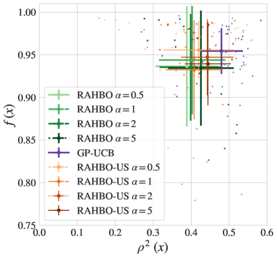
Refer to caption
(a)
Refer to caption
(b)
Refer to caption
(c)
Figure 10: (a) We plot standard deviation error bars for f(x)𝑓𝑥f(x) and ρ2(x)superscript𝜌2𝑥\rho^{2}(x) at the reported point by the best observed value x(T)=argmaxxtyt(xt)superscript𝑥𝑇subscriptargmaxsubscript𝑥𝑡subscript𝑦𝑡subscript𝑥𝑡x^{(T)}=\operatorname*{arg\,max}_{x_{t}}y_{t}(x_{t}) after BO completion for SwissFEL. The mean and std of the error bars are taken over the repeated BO experiments. The results demonstrate, that reporting based on the best observed value inherits high noise and as the result all methods perform similarly. Intuitively, when noise variance is high, it is possible to observe higher values. That however also inherits observing much lower value at this point, this leading to very non-robust solutions. (b-c) Cumulative regret for α=2𝛼2\alpha=2 and α=5𝛼5\alpha=5.