NAS-Bench-x11 and the Power of Learning Curves

Abstract

While early research in neural architecture search (NAS) required extreme computational resources, the recent releases of tabular and surrogate benchmarks have greatly increased the speed and reproducibility of NAS research. However, two of the most popular benchmarks do not provide the full training information for each architecture. As a result, on these benchmarks it is not possible to run many types of multi-fidelity techniques, such as learning curve extrapolation, that require evaluating architectures at arbitrary epochs. In this work, we present a method using singular value decomposition and noise modeling to create surrogate benchmarks, NAS-Bench-111, NAS-Bench-311, and NAS-Bench-NLP11, that output the full training information for each architecture, rather than just the final validation accuracy. We demonstrate the power of using the full training information by introducing a learning curve extrapolation framework to modify single-fidelity algorithms, showing that it leads to improvements over popular single-fidelity algorithms which claimed to be state-of-the-art upon release. Our code and pretrained models are available at https://github.com/automl/nas-bench-x11.

1 Introduction

In the past few years, algorithms for neural architecture search (NAS) have been used to automatically find architectures that achieve state-of-the-art performance on various datasets [82, 53, 38, 13]. In 2019, there were calls for reproducible and fair comparisons within NAS research [34, 57, 75, 36] due to both the lack of a consistent training pipeline between papers and experiments with not enough trials to reach statistically significant conclusions. These concerns spurred the release of tabular benchmarks, such as NAS-Bench-101 [76] and NAS-Bench-201 [11], created by fully training all architectures in search spaces of size $423\,624$ and $6\,466$, respectively. These benchmarks allow researchers to easily simulate NAS experiments, making it possible to run fair NAS comparisons and to run enough trials to reach statistical significance at very little computational cost or carbon emissions [17]. Recently, to extend the benefits of tabular NAS benchmarks to larger, more realistic NAS search spaces which cannot be evaluated exhaustively, it was proposed to construct surrogate benchmarks [60]. The first such surrogate benchmark is NAS-Bench-301 [60], which models the DARTS [38] search space of size $10^{18}$ architectures. It was created by fully training $60\,000$ architectures (both drawn randomly and chosen by top NAS methods) and then fitting a surrogate model that can estimate the performance of all of the remaining architectures. Since 2019, dozens of papers have used these NAS benchmarks to develop new algorithms [67, 55, 73, 64, 59].

An unintended side-effect of the release of these benchmarks is that it became significantly easier to devise single fidelity NAS algorithms: when the NAS algorithm chooses to evaluate an architecture, the architecture is fully trained and only the validation accuracy at the final epoch of training is outputted. This is because NAS-Bench-301 only contains the architectures’ accuracy at epoch 100, and NAS-Bench-101 only contains the accuracies at epochs 4, 12, 36, and 108 (allowing single fidelity or very limited multi-fidelity approaches). NAS-Bench-201 does allow queries on the entire learning curve (every epoch), but it is smaller in size ($6\,466$) than NAS-Bench-101 ($423\,624$) or NAS-Bench-301 ($10^{18}$). In a real world experiment, since training architectures to convergence is computationally intensive, researchers will often run multi-fidelity algorithms: the NAS algorithm can train architectures to any desired epoch. Here, the algorithm can make use of speedup techniques such as learning curve extrapolation (LCE) [63, 8, 1, 28] and successive halving [35, 14, 32, 29]. Although multi-fidelity techniques are often used in the hyperparameter optimization community [20, 21, 35, 14, 63], they have been under-utilized by the NAS community in the last few years.

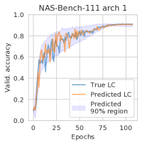
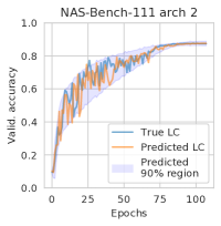
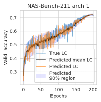
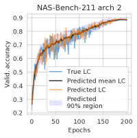
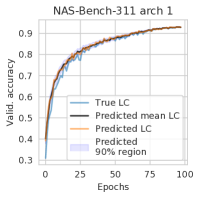
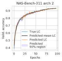
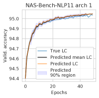
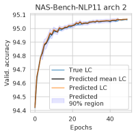
In this work, we fill in this gap by releasing NAS-Bench-111, NAS-Bench-311, and NAS-Bench-NLP11, surrogate benchmarks with full learning curve information for train, validation, and test loss and accuracy for all architectures, significantly extending NAS-Bench-101, NAS-Bench-301, and NAS-Bench-NLP [30], respectively. With these benchmarks, researchers can easily incorporate multi-fidelity techniques, such as early stopping and LCE into their NAS algorithms. Our technique for creating these benchmarks can be summarized as follows. We use a training dataset of architectures (drawn randomly and chosen by top NAS methods) with good coverage over the search space, along with full learning curves, to fit a model that predicts the full learning curves of the remaining architectures. We employ three techniques to fit the model: (1) dimensionality reduction of the learning curves, (2) prediction of the top singular value coefficients, and (3) noise modeling. These techniques can be used in the future to create new NAS benchmarks as well. To ensure that our surrogate benchmarks are highly accurate, we report statistics such as Kendall Tau rank correlation and Kullback Leibler divergence between ground truth learning curves and predicted learning curves on separate test sets. See Figure 1 for examples of predicted learning curves on the test sets.

Figure 1: Each image shows the true learning curve vs. the learning curve predicted by our surrogate models, with and without predicted noise modeling. We also plot the 90% confidence interval of the predicted noise distribution. We plot two architectures each for NAS-Bench-111, NAS-Bench-211, NAS-Bench-311, and NAS-Bench-NLP11.

To demonstrate the power of using the full learning curve information, we present a framework for converting single-fidelity NAS algorithms into multi-fidelity algorithms using LCE. We apply our framework to popular single-fidelity NAS algorithms, such as regularized evolution [53], local search [68], and BANANAS [67], all of which claimed state-of-the-art upon release, showing that they can be further improved across four search spaces. Finally, we also benchmark multi-fidelity algorithms such as Hyperband [35] and BOHB [14] alongside single-fidelity algorithms. Overall, our work bridges the gap between different areas of AutoML and will allow researchers to easily develop effective multi-fidelity and LCE techniques in the future. To promote reproducibility, we release our code and we follow the NAS best practices checklist [36], providing the details in Appendix A.

Our contributions. We summarize our main contributions below.

• We develop a technique to create surrogate NAS benchmarks that include the full training information for each architecture, including train, validation, and test loss and accuracy learning curves. This technique can be used to create future NAS benchmarks on any search space.

• We apply our technique to create NAS-Bench-111, NAS-Bench-311, and NAS-Bench-NLP11, which allow researchers to easily develop multi-fidelity NAS algorithms that achieve higher performance than single-fidelity techniques.

• We present a framework for converting single-fidelity NAS algorithms into multi-fidelity NAS algorithms using learning curve extrapolation, and we show that our framework allows popular state-of-the-art NAS algorithms to achieve further improvements.

2 Related Work

NAS has been studied since at least the late 1980s [43, 26, 62] and has recently seen a resurgence [82, 44, 52, 22, 53, 18]. Weight sharing algorithms have become popular due to their computational efficiency [2, 38, 10, 79, 77, 51, 78]. Recent advances in performance prediction [65, 46, 59, 74, 39, 69, 55, 67] and other iterative techniques [14, 45] have reduced the runtime gap between iterative and weight sharing techniques. For detailed surveys on NAS, we suggest referring to [13, 71].

Learning curve extrapolation.

Several methods have been proposed to estimate the final validation accuracy of a neural network by extrapolating the learning curve of a partially trained neural network. Techniques include fitting the partial curve to an ensemble of various parametric functions [8], predicting the performance based on the derivatives of the learning curves of partially trained neural network configurations [1], summing the training losses [54], using the basis functions as the output layer of a Bayesian neural network [28], using previous learning curves as basis function extrapolators [4], using the positive-definite covariance kernel to capture a variety of training curves [63], or using a Bayesian recurrent neural network [15]. While in this work we focus on multi-fidelity optimization utilizing learning curve-based extrapolation, another main category of methods lie in bandit-based algorithm selection [35, 14, 29, 19, 40], and the fidelities can be further adjusted according to the previous observations or a learning rate scheduler [20, 21, 27].

Table 1: Overview of existing NAS benchmarks. We introduce NAS-Bench-111, -311, and -NLP11.

Benchmark	Size	Queryable	Based on	Full train info
NAS-Bench-101	423k	✓		✗
NAS-Bench-201	6k	✓		✓
NAS-Bench-301	$10^{18}$	✓	DARTS	✗
NAS-Bench-NLP	$10^{53}$	✗		✗
NAS-Bench-ASR	8k	✓		✓
NAS-Bench-111	423k	✓	NAS-Bench-101	✓
NAS-Bench-311	$10^{18}$	✓	DARTS	✓
NAS-Bench-NLP11	$10^{53}$	✓	NAS-Bench-NLP	✓

NAS benchmarks.

NAS-Bench-101 [76], a tabular NAS benchmark, was created by defining a search space of size $423\,624$ unique architectures and then training all architectures from the search space on CIFAR-10 until 108 epochs. However, the train, validation, and test accuracies are only reported for epochs 4, 12, 36, and 108, and the training, validation, and test losses are not reported. NAS-Bench-1shot1 [80] defines a subset of the NAS-Bench-101 search space that allows one-shot algorithms to be run. NAS-Bench-201 [11] contains $15\,625$ architectures, of which $6\,466$ are unique up to isomorphisms. It comes with full learning curve information on three datasets: CIFAR-10 [31], CIFAR-100 [31], and ImageNet16-120 [7]. Recently, NAS-Bench-201 was extended to NATS-Bench [9] which searches over architecture size as well as architecture topology.

Virtually every published NAS method for image classification in the last three years evaluates on the DARTS search space with CIFAR-10 [61]. The DARTS search space  [38] consists of $10^{18}$ neural architectures, making it computationally prohibitive to create a tabular benchmark. To overcome this fundamental limitation and query architectures in this much larger search space, NAS-Bench-301 [60] evaluates various regression models trained on a sample of $60\,000$ architectures that is carefully created to cover the whole search space. The surrogate models allow users to query the validation accuracy (at epoch 100) and training time for any of the $10^{18}$ architectures in the DARTS search space. However, since the surrogates do not predict the entire learning curve, it is not possible to run multi-fidelity algorithms.

NAS-Bench-NLP [30] is a search space for language modeling tasks. The search space consists of $10^{53}$ architectures, of which $14\,322$ are evaluated on Penn Tree Bank [42], containing the training, validation, and test losses/accuracies from epochs 1 to 50. Since only $14\,322$ of $10^{53}$ architectures can be queried, this dataset cannot be directly used for NAS experiments. NAS-Bench-ASR [41] is a recent tabular NAS benchmark for speech recognition. The search space consists of $8\,242$ architectures with full learning curve information. For an overview of NAS benchmarks, see Table 1.

3 Creating Surrogate Benchmarks with Learning Curves

In this section, we describe our technique to create a surrogate model that outputs realistic learning curves, and then we apply this technique to create NAS-Bench-111, NAS-Bench-311, and NAS-Bench-NLP11. Our technique applies to any type of learning curve, including train/test losses and accuracies. For simplicity, the following presentation assumes validation accuracy learning curves.

3.1 General Technique

Figure 2: A summary of our approach to create surrogate benchmarks that output realistic learning curves. Compression and decompression functions are learned using the training set of learning curves (in the figure, SVD is shown, but a VAE can also be used). The compression also helps to de-noise the learning curves. A model ($\mu$-model) is trained to predict the compressed (de-noised) learning curves given the architecture encoding. A separate model ($\Sigma$-model) is trained to predict each learning curve’s noise distribution, given the architecture encoding and predicted compressed learning curve. A realistic learning curve can then be outputted by decompressing the predicted learning curve and sampling noise from the noise distribution.

Given a search space $\mathcal{D}$, let $(\bm{x}_{i},\bm{y}_{i})\sim\mathcal{D}$ denote one datapoint, where $\bm{x}_{i}\in\mathbb{R}^{d}$ is the architecture encoding (e.g., one-hot adjacency matrix [76, 66]), and $\bm{y}_{i}\in[0,1]^{E_{\text{max}}}$ is a learning curve of validation accuracies drawn from a distribution $Y(\bm{x}_{i})$ based on training the architecture for $E_{\text{max}}$ epochs on a fixed training pipeline with a random initial seed. Without loss of generality, each learning curve $\bm{y}_{i}$ can be decomposed into two parts: one part that is deterministic and depends only on the architecture encoding, and another part that is based on the inherent noise in the architecture training pipeline. Formally, $\bm{y}_{i}=\mathbb{E}[Y(\bm{x}_{i})]+\bm{\epsilon}_{i}$, where $\mathbb{E}[Y(\bm{x}_{i})]\in[0,1]^{E_{\text{max}}}$ is fixed and depends only on $\bm{x}_{i}$, and $\bm{\epsilon}_{i}\in[0,1]^{E_{\text{max}}}$ comes from a noise distribution $Z_{i}$ with expectation 0 for all epochs. In practice, $\mathbb{E}[Y(\bm{x}_{i})]$ can be estimated by averaging a large set of learning curves produced by training architecture $\bm{x}_{i}$ with different initial seeds. We represent such an estimate as $\bar{\bm{y}}_{i}$.

Our goal is to create a surrogate model that takes as input any architecture encoding $\bm{x}_{i}$ and outputs a distribution of learning curves that mimics the ground truth distribution. We assume that we are given two datasets, $\mathcal{D}_{\text{train}}$ and $\mathcal{D}_{\text{test}}$, of architecture and learning curve pairs. We use $\mathcal{D}_{\text{train}}$ (often size $>10\,000$) to train the surrogate, and we use $\mathcal{D}_{\text{test}}$ for evaluation. We describe the process of creating $\mathcal{D}_{\text{train}}$ and $\mathcal{D}_{\text{test}}$ for specific search spaces in the next section. In order to predict a learning curve distribution for each architecture, we split up our approach into two separate processes: we train a model $f:\mathbb{R}^{d}\to[0,1]^{E_{\text{max}}}$ to predict the deterministic part of the learning curve, $\bar{\bm{y}}_{i}$, and we train a noise model $p_{\phi}(\bm{\epsilon}\mid\bar{\bm{y}},\bm{x})$, parameterized by $\phi$, to simulate the random draws from $Z_{i}$.

Surrogate model training.

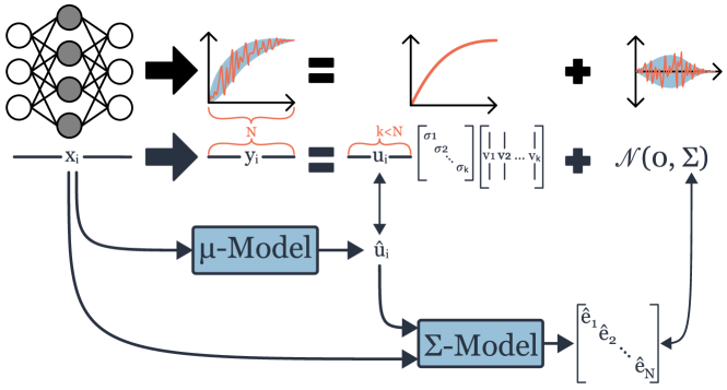
Training a model $f$ to predict mean learning curves is a challenging task, since the training datapoints $\mathcal{D}_{\text{train}}$ consist only of a single (or few) noisy learning curve(s) $\bm{y}_{i}$ for each $\bm{x}_{i}$. Furthermore, $E_{\text{max}}$ is typically length 100 or larger, meaning that $f$ must predict a high-dimensional output. We propose a technique to help with both of these challenges: we use the training data to learn compression and decompression functions $c_{k}:[0,1]^{E_{\text{max}}}\rightarrow[0,1]^{k}$ and $d_{k}:[0,1]^{k}\rightarrow[0,1]^{E_{\text{max}}}$, respectively, for $k\ll E_{\text{max}}$. The surrogate is trained to predict compressed learning curves $c_{k}\left(\bm{y}_{i}\right)$ of size $k$ from the corresponding architecture encoding $\bm{x}_{i}$, and then each prediction can be reconstructed to a full learning curve using $d_{k}$. A good compression model should not only cause the surrogate prediction to become significantly faster and simpler, but should also reduce the noise in the learning curves, since it would only save the most important information in the compressed representations. That is, $(d_{k}\circ c_{k})\left(\bm{y}_{i}\right)$ should be a less noisy version of $\bm{y}_{i}$. Therefore, models trained on $c_{k}\left(\bm{y}_{i}\right)$ tend to have better generalization ability and do not overfit to the noise in individual learning curves.

Figure 3: The singular values from the SVD decomposition of the learning curves (LC) (left). The MSE of a reconstructed LC, showing that $k=6$ is closest to the true mean LC, while larger values of $k$ overfit to the noise of the LC (middle). An LC reconstructed using different values of $k$ (right).

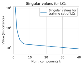
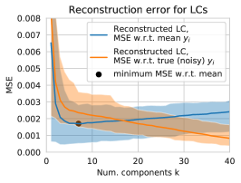
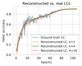
We test two compression techniques: singular value decomposition (SVD) [16] and variational autoencoders (VAEs) [25], and we show later that SVD performs better. We give the details of SVD here and describe the VAE compression algorithm in Appendix C. Formally, we take the singular value decomposition of a matrix $S$ of dimension $(|\mathcal{D}_{\text{train}}|,E_{\text{max}})$ created by stacking together the learning curves from all architectures in $\mathcal{D}_{\text{train}}$. Performing the truncated SVD on the learning curve matrix $S$ allow us to create functions $c_{k}$ and $d_{k}$ that correspond to the optimal linear compression of $S$. In Figure 3 (left), we see that for architectures in the NAS-Bench-101 search space, there is a steep dropoff of importance after the first six singular values, which intuitively means that most of the information for each learning curve is contained in its first six singular values. In Figure 3 (middle), we compute the mean squared error (MSE) of the reconstructed learning curves $(d_{k}\circ c_{k})\left(\bm{y}_{i}\right)$ compared to a test set of ground truth learning curves averaged over several initial seeds (approximating $\mathbb{E}[Y(\bm{x}_{i})]$). The lowest MSE is achieved at $k=6$, which implies that $k=6$ is the value where the compression function minimizes reconstruction error without overfitting to the noise of individual learning curves. We further validate this in Figure 3 (right) by plotting $(d_{k}\circ c_{k})\left(\bm{y}_{i}\right)$ for different values of $k$. Now that we have compression and decompression functions, we train a surrogate model with $\bm{x}_{i}$ as features and $c_{k}\left(\bm{y}_{i}\right)$ as the label, for architectures in $\mathcal{D}_{\text{train}}$. We test LGBoost [23], XGBoost [5], and MLPs for the surrogate model.

Noise modeling.

The final step for creating a realistic surrogate benchmark is to add a noise model, so that the outputs are noisy learning curves. We first create a new dataset of predicted $\bm{\epsilon}_{i}$ values, which we call residuals, by subtracting the reconstructed mean learning curves from the real learning curves in $\mathcal{D}_{\text{train}}$. That is, $\hat{\bm{\epsilon}}_{i}=\bm{y}_{i}-(d_{k}\circ c_{k})\left(\bm{y}_{i}\right)$ is the residual for the $i$th learning curve. Since the training data only contains one (or few) learning curve(s) per architecture $\bm{x}_{i}$, it is not possible to accurately estimate the distribution $Z_{i}$ for each architecture without making further assumptions. We assume that the noise comes from an isotropic Gaussian distribution, and we consider two other noise assumptions: (1) the noise distribution is the same for all architectures (to create baselines, or for very homogeneous search spaces), and (2) for each architecture, the noise in a small window of epochs are iid. In Appendix C, we estimate the extent to which all of these assumptions hold true. Assumption (1) suggests two potential (baseline) noise models: (i) a simple sample standard deviation statistic, $\bm{\sigma}\in\mathbb{R}_{+}^{E_{\text{max}}}$, where

$$\sigma_{j}=\sqrt{\frac{1}{|\mathcal{D}_{\text{train}}|-1}\sum_{i=1}^{|\mathcal{D}_{\text{train}}|}\hat{\epsilon}_{i,j}^{2}}.$$

To sample the noise using this model, we sample from $\mathcal{N}(\bm{0},\text{diag}(\bm{\sigma}))$. (ii) The second model is a Gaussian kernel density estimation (GKDE) model [58] trained on the residuals to create a multivariate Gaussian kernel density estimate for the noise. Assumption (2) suggests one potential noise model: (iii) a model that is trained to estimate the distribution of the noise over a window of epochs of a specific architecture. For each architecture and each epoch, the model is trained to estimate the sample standard deviation of the residuals within a window centered around that epoch.

See Figure 2 for a summary of the entire surrogate creation method (assuming SVD). Throughout this section, we described two compression methods (SVD and VAE), three surrogate models (LGB, XGB, and MLP), and three noise models (stddev, GKDE, and sliding window), for a total of eighteen disctinct approaches. In the next section, we describe the methods we will use to evaluate these approaches.

3.2 Surrogate Benchmark Evaluation

The performance of a surrogate benchmark depends on factors such as the size of the training set of architecture + learning curve pairs, the length of the learning curves, and the extent to which the distribution of learning curves satisfy the noise assumptions discussed in the previous section. It is important to thoroughly evaluate surrogate benchmarks before their use in NAS research, and so we present a number of different methods for evaluation, which we will use to evaluate the surrogate benchmarks we create in the next section.

We evaluate both the predicted mean learning curves and the predicted noise distributions using held-out test sets $\mathcal{D}_{\text{test}}$. To evaluate the mean learning curves, we compute the coefficient of determination ($R^{2}$) [70] and Kendall Tau (KT) rank correlation [24] between the set of predicted mean learning curves and the set of true learning curves, both at the final epoch and averaged over all epochs. To measure KT rank correlation for a specific epoch $n$, we find the number of concordant, $P$, and discordant, $Q$, pairs of predicted and true learning curve values for that epoch. The number of concordant pairs is given by the number of pairs, $((\hat{y}_{i,n},y_{i,n}),(\hat{y}_{j,n},y_{j,n}))$, where either both $\hat{y}_{i,n}>\hat{y}_{j,n}$ and $y_{i,n}>y_{j,n}$, or both $\hat{y}_{i,n}<\hat{y}_{j,n}$ and $y_{j,n}<y_{i,n}$. We can then calculate $KT=\frac{P-Q}{P+Q}$. While these metrics can be used to compare surrogate predictions and have been used in prior work [60], the rank correlation values are affected by the inherent noise in the learning curves - even an oracle would have $R^{2}$ and KT values smaller than 1.0 because architecture training is noisy. In order to give reference values, we also compute the KT of the set of true learning curves averaged over 2, 3, or 4 independent random seeds.

The next metric to be used in Section 3.3 is the Kullback Leibler (KL) divergence between the ground truth distribution of noisy learning curves, and the predicted distribution of noisy learning curves on a test set. Since we can only estimate the ground truth distribution, we assume the ground truth is an isotropic Gaussian distribution. Then we measure the KL divergence between the true and predicted learning curves for architecture $i$ by the following formula:

$$D_{KL}(\bm{y}_{i}||\hat{\bm{y}}_{i})=\frac{1}{2E_{\text{max}}}\left[\log\frac{|\Sigma_{\hat{\bm{y}}_{i}}|}{|\Sigma_{\bm{y}_{i}}|}-E_{\text{max}}+(\bm{\mu_{\bm{y}_{i}}}-\bm{\mu_{\hat{\bm{y}}_{i}}})^{T}\Sigma_{\hat{\bm{y}}_{i}}^{-1}(\bm{\mu_{\bm{y}_{i}}}-\bm{\mu_{\hat{\bm{y}}_{i}}})+tr\left\{\Sigma_{\hat{\bm{y}}_{i}}^{-1}\Sigma_{\bm{y}_{i}}\right\}\right]$$

where $\Sigma_{\{\bm{y}_{i},\hat{\bm{y}}_{i}\}}$ is a diagonal matrix with the entries ${\Sigma_{\{\bm{y}_{i},\hat{\bm{y}}_{i}\}}}_{k,k}$ representing the sample variance of the $k$-th epoch, and $\bm{\mu}_{\{\bm{y}_{i},\hat{\bm{y}}_{i}\}}$ is the sample mean for either learning curves $\{\bm{y}_{i},\hat{\bm{y}}_{i}\}$.

The final metric is the probability of certain anomalies which we call spike anomalies. Even if the KL divergences between the surrogate benchmark distributions and the ground-truth distributions are low, anomalies in the learning curves can still throw off NAS algorithms. For example, there may be anomalies that cause some learning curves to have a much higher maximum validation accuracy than their final validation accuracy. In order to test for these anomalies, first we compute the largest value $x$ such that there are fewer than 5% of learning curves whose maximum validation accuracy is $x$ higher than their final validation accuracy, on the real set of learning curves. Then, we compute the percentage of surrogate learning curves whose maximum validation accuracy is $x$ higher than their final validation accuracy. The goal is for this value to be close to 5%.

3.3 Creating NAS-Bench-111, -211, -311, and -NLP11

Now we describe the creation of NAS-Bench-111, NAS-Bench-311, and NAS-Bench-NLP11. We also create NAS-Bench-211 purely to evaluate our technique (since NAS-Bench-201 already has complete learning curves). Our code and pretrained models are available at https://github.com/automl/nas-bench-x11. As described above, we test two different compression methods (SVD, VAE), three different surrogate models (LGB, XGB, MLP), and three different noise models (stddev, GKDE, sliding window) for a total of eighteen distinct approaches. See Appendix C for a full ablation study and Table 2 for a summary using the best techniques for each search space. See Figure 1 for a visualization of predicted learning curves from the test set of each search space using these models.

First, we describe the creation of NAS-Bench-111. Since the NAS-Bench-101 tabular benchmark [76] consists only of accuracies at epochs 4, 12, 36, and 108 (and without losses), we train a new set of architectures and save the full learning curves. Similar to prior work [12, 60], we sample a set of architectures with good overall coverage while also focusing on the high-performing regions exploited by NAS algorithms. Specifically, we sample 861 architectures generated uniformly at random, 149 architectures generated by 30 trials of BANANAS, local search, and regularized evolution, and all 91 architectures which contain fewer than five nodes, for a total of 1101 architectures. We kept our training pipeline as close as possible to the original pipeline. See Appendix C for the full training details. We find that SVD-LGB-window and SVD-LGB-GKDE achieve the best performance. Since the tabular benchmark already exists, we can substantially improve the accuracy of our surrogate by using the accuracies from the tabular benchmark (at epochs 4, 12, 36, 108) as additional features along with the architecture encoding. This substantially improves the performance of the surrogate, as shown in Table 2. The large difference between the average KT and last epoch KT values show that the learning curves are very noisy (which is also evidenced in Figure 1). On a separate test set that contains two seeds evaluated per architecture, we show that the KT values for NAS-Bench-111 are roughly equivalent to those achieved by a 1-seed tabular benchmark (Appendix Table 4).

Next, we create NAS-Bench-311 by using the training data from NAS-Bench-301, which consists of $40\,000$ random architectures along with $26\,000$ additional architectures generated by evolution [53], Bayesian optimization [3, 67, 47], and one-shot [38, 72, 10, 6] techniques in order to achieve good coverage over the search space. SVD-LGB-GKDE achieves the best performance. The GKDE model performing well is consistent with prior work that notes DARTS is very homogeneous [75]. NAS-Bench-311 achieves average and last epoch KT values of 0.728 and 0.788, respectively. This is comparable to the last epoch KT of 0.817 reported by NAS-Bench-301 [60], despite optimizing for the full learning curve rather than only the final epoch. Furthermore, our KL divergences in Table 2 surpasses the top value of 16.4 reported by NAS-Bench-301 (for KL divergence, lower is better). In Appendix Table 5, we show that the mean model in NAS-Bench-311 achieves higher rank correlation even than a set of learning curves averaged over four random seeds, by using a separate test set from the NAS-Bench-301 dataset which evaluates 500 architectures with 5 seeds each. We also show that the percentage of spike anomalies for real vs. surrogate data (defined in the previous section) is 5% and 7.02%, respectively.

Finally, we create NAS-Bench-NLP11 by using the NAS-Bench-NLP dataset consisting of $14\,322$ architectures drawn uniformly at random. Due to the extreme size of the search space ($10^{53}$), we achieve an average and final epoch KT of 0.449 and 0.416, respectively. Since there are no architectures trained multiple times on the NAS-Bench-NLP dataset [30], we cannot compute the KL divergence or additional metrics. To create a stronger surrogate, we add the first three epochs of the learning curve as features in the surrogate. This improves the average and final epoch KT values to 0.862 and 0.820, respectively. To use this surrogate, any architecture to be predicted with the surrogate must be trained for three epochs. Note that the small difference between the average and last epoch KT values indicates that the learning curves have very little noise, which can also be seen in Figure 1. This technique can be used to improve the performance of other surrogates too, such as NAS-Bench-311. For NAS-Bench-311, we find that adding the validation accuracies from the first three epochs as additional epochs, improves the average and final epoch KT from 0.728 and 0.788 to 0.749 and 0.795, respectively.

We also create NAS-Bench-211 to further evaluate our surrogate creation technique (only for evaluation purposes, since NAS-Bench-201 already has complete learning curves). We train the surrogate on 90% of architectures from NAS-Bench-201 (14 062 architectures) and test on the remaining 10%. SVD-LGB-window achieves the best performance. The average and final KT values are 0.701 and 0.842, respectively, which is on par with a 1-seed tabular benchmark (see Table 6). We also show that the percentage of spike anomalies for real vs. surrogate data (defined in the previous section) is 5% and 10.14%, respectively.

Table 2: Evaluation of the surrogate benchmarks on test sets. For NAS-Bench-111 and NAS-Bench-NLP11, we use architecture accuracies as additional features to improve performance.

Benchmark	Avg. $R^{2}$	Final $R^{2}$	Avg. KT	Final KT	Avg. KL	Final KL
NAS-Bench-111	0.529	0.630	0.531	0.645	2.016	1.061
NAS-Bench-111 (w. accs)	0.630	0.853	0.611	0.794	1.710	0.926
NAS-Bench-311	0.779	0.800	0.728	0.788	0.905	0.600
NAS-Bench-NLP11	0.327	0.292	0.449	0.416	-	-
NAS-Bench-NLP11 (w. accs)	0.906	0.882	0.862	0.820	-	-

4 The Power of Learning Curve Extrapolation

Now we describe a simple framework for converting single-fidelity NAS algorithms to multi-fidelity NAS algorithms using learning curve extrapolation techniques. We show that this framework is able to substantially improve the performance of popular algorithms such as regularized evolution [53], BANANAS [67], and local search [68, 48].

A single-fidelity algorithm is an algorithm which iteratively chooses an architecture based on its history, which is then fully trained to $E_{\text{max}}$ epochs. To exploit parallel resources, many single-fidelity algorithms iteratively output several architectures at a time, instead of just one. In Algorithm 1, we present pseudocode for a generic single-fidelity algorithm. For example, for local search, gen_candidates would output the neighbors of the architecture with the best accuracy in history.

Our framework makes use of learning curve extrapolation (LCE) techniques [8, 1] to predict the final validation accuracies of all architecture choices after only training for a small number of epochs. See Algorithm 2. After each iteration of gen_candidates, only the architectures predicted by LCE() to be in the top percentage of validation accuracies of history are fully trained. For example, when the framework is applied to local search, in each iteration, all neighbors are trained to $E_{\text{few}}$ epochs, and only the most promising architectures are trained up to $E_{\text{max}}$ epochs. This simple modification can substantially improve the runtime efficiency of popular NAS algorithms by weeding out unpromising architectures before they are fully trained.

Any LCE technique can be used, and in our experiments in Section 5, we use weighted probabilistic modeling (WPM) [8] and learning curve support vector regressor (LcSVR) [1]. The first technique, WPM [8], is a function that takes a partial learning curve as input, and then extrapolates it by fitting the learning curve to a set of parametric functions, using MCMC to sample the most promising fit. The second technique, LcSVR [1], is a model-based learning curve extrapolation technique: after generating an initial set of training architectures, a support vector regressor is trained to predict the final validation accuracy from the architecture encoding and partial learning curve.

Algorithm 1 Single-Fidelity Algorithm

1:  initialize history

2:  while $t<t_{\max}:$

3:   arches = gen_candidates(history)

4:   accs = train(arches, epoch=$E_{\text{max}}$)

5:   history.update(arches, accs)

6:  Return arch with the highest acc

Algorithm 2 LCE Framework

1:  initialize history

2:  while $t<t_{\max}:$

3:   arches = gen_candidates(history)

4:   accs = train(arches, epoch=$E_{\text{few}}$)

5:   sorted_by_pred = LCE(arches, accs)

6:   arches = sorted_by_pred[:top_n]

7:   accs = train(arches, epoch=$E_{\text{max}}$)

8:   history.update(arches, accs)

9:  Return arch with the highest acc

5 Experiments

In this section, we benchmark single-fidelity and multi-fidelity NAS algorithms, including popular existing single-fidelity and multi-fidelity algorithms, as well as algorithms created using our framework defined in the previous section. In the experiments, we use our three surrogate benchmarks defined in Section 3, as well as NAS-Bench-201.

NAS algorithms.

For single-fidelity algorithms, we implemented random search (RS) [34], local search (LS) [68, 48], regularized evolution (REA) [53], and BANANAS [67]. For multi-fidelity bandit-based algorithms, we implemented Hyperband (HB) [35] and Bayesian optimization Hyperband (BOHB) [14]. For all methods, we use the original implementation whenever possible. See Appendix D for a description, implementation details, and hyperparameter details for each method. Finally, we use our framework from Section 4 to create six new multi-fidelity algorithms: BANANAS, LS, and REA are each augmented using WPM and LcSVR. This gives us a total of $12$ algorithms.

Experimental setup.

For each search space, we run each algorithm for a total wall-clock time that is equivalent to running 500 iterations of the single-fidelity algorithms for NAS-Bench-111 and NAS-Bench-311, and 100 iterations for NAS-Bench-201 and NAS-Bench-NLP11. For example, the average time to train a NAS-Bench-111 architecture to 108 epochs is roughly $10^{3}$ seconds, so we set the maximum runtime on NAS-Bench-111 to roughly $5\cdot 10^{5}$ seconds. We run 30 trials of each NAS algorithm and compute the mean and standard deviation.

Figure 4: LCE Framework applied to single-fidelity algorithms on NAS-Bench-311.

Results.

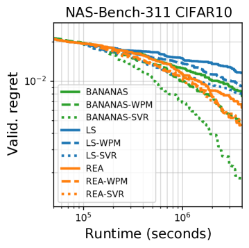
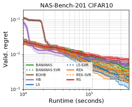
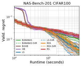
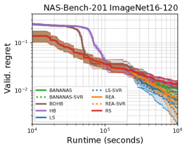
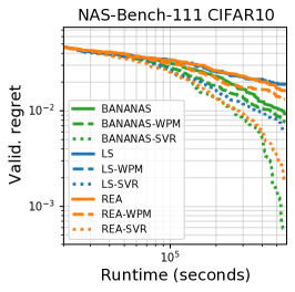
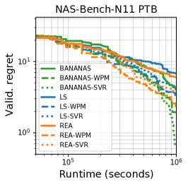
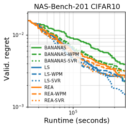
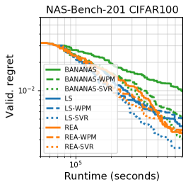
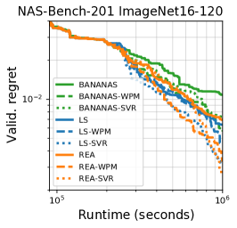
We evaluate BANANAS, LS, and REA compared to their augmented WPM and SVR versions in Figure 4 (NAS-Bench-311) and Appendix D (all other search spaces). Across four search spaces, we see that WPM and SVR improve all algorithms in almost all settings. The improvements are particularly strong for the larger NAS-Bench-111 and NAS-Bench-311 search spaces. We also see that for each single-fidelity algorithm, the LcSVR variant often outperforms the WPM variant. This suggests that model-based techniques for extrapolating learning curves are more reliable than extrapolating each learning curve individually, which has also been noted in prior work [69].

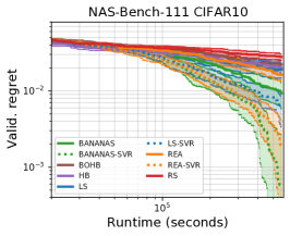
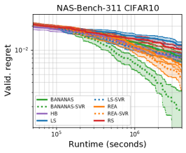
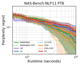
In Figure 5, we compare single- and multi-fidelity algorithms on four search spaces, along with the three SVR-based algorithms from Figure 4. Across all search spaces, an SVR-based algorithm is the top-performing algorithm. Specifically, BANANAS-SVR performs the best on NAS-Bench-111, NAS-Bench-311, and NAS-Bench-NLP11, and LS-SVR performs the best on NAS-Bench-201. Note that HB and BOHB may not perform well on search spaces with low correlation between the relative rankings of architectures using low fidelities and high fidelities (such as NAS-Bench-101 [76] and NAS-Bench-201 [11]) since HB-based methods will predict the final accuracy of partially trained architectures directly from the last trained accuracy (i.e., extrapolating the learning curve as a constant after the last seen accuracy). On the other hand, SVR-based approaches use a model that can learn more complex relationships between accuracy at an early epoch vs. accuarcy at the final epoch, and are therefore more robust to this type of search space.

In Appendix D, we perform an ablation study on the epoch at which the SVR and WPM methods start extrapolating in our framework (i.e., we ablate $E_{\text{few}}$ from Algorithm 2). We find that for most search spaces, running SVR and WPM based NAS methods by starting the LCE at roughly $20\%$ of the total number of epochs performs the best. Any earlier, and there is not enough information to accurately extrapolate the learning curve. Any later, and the LCE sees diminishing returns because less time is saved by early stopping the training.

Figure 5: NAS results on six different combinations of search spaces and datasets. For every setting, an SVR augmented method performs best.

6 Societal Impact

Our hope is that our work will make it quicker and easier for researchers to run fair experiments and give reproducible conclusions. In particular, the surrogate benchmarks allow AutoML researchers to develop NAS algorithms directly on a CPU, as opposed to using a GPU, which may decrease the carbon emissions from GPU-based NAS research [50, 17]. In terms of our proposed NAS speedups, these techniques are a level of abstraction away from real applications, but they can indirectly impact the broader society. For example, this work may facilitate the creation of new high-performing NAS techniques, which can then be used to improve various deep learning methods, both beneficial (e.g. algorithms that reduce $\text{CO}_{2}$ emissions), or harmful (e.g. algorithms that produce deep fakes).

7 Conclusions, Limitations, and Guidelines

In this work, we released three benchmarks for neural architecture search based on three popular search spaces, which substantially improve the capability of existing benchmarks due to the availability of the full learning curve for train/validation/test loss and accuracy for each architecture. Our techniques to generate these benchmarks, which includes singular value decomposition of the learning curve and noise modeling, can be used to model the full learning curve for future surrogate NAS benchmarks as well.

Furthermore, we demonstrated the power of the full learning curve information by introducing a framework that converts single-fidelity NAS algorithms into multi-fidelity NAS algorithms that make use of learning curve extrapolation techniques. This framework improves the performance of recent popular single-fidelity algorithms which claimed to be state-of-the-art upon release.

While we believe our surrogate benchmarks will help advance scientific research in NAS, a few guidelines and limitations are important to keep in mind. As with prior surrogate benchmarks [60], we give the following two caveats. (1) We discourage evaluating NAS methods that use the same internal techniques as those used in the surrogate model. For example, any NAS method that makes use of variational autoencoders or XGBoost should not be benchmarked using our VAE-XGB surrogate benchmark. (2) As the surrogate benchmarks are likely to evolve as new training data is added, or as better techniques for training a surrogate are devised, we recommend reporting the surrogate benchmark version number whenever running experiments. (3) When creating new surrogate benchmarks, before use in NAS, it is important to give a thorough evaluation such as the evaluation methods described in Section 3.2.

We also note the following strengths and limitations for specific benchmarks. Our NAS-Bench-111 surrogate benchmark gives strong mean performance even with just $1\,101$ architectures used as training data, due to the existence of the four extra validation accuracies from NAS-Bench-101 that can be used as additional features. We hope that all future tabular benchmarks will save the full learning curve information from the start so that the creation of an after-the-fact extended benchmark is not necessary.

Although all of our surrogates had strong mean performance, the noise model was strongest only for NAS-Bench-311, which had a training dataset of size 60k, as evidenced especially because of the rate of spike anomalies, described in Section 3.2. This can be mitigated by adding more training data.

Since the NAS-Bench-NLP11 surrogate benchmark achieves significantly stronger performance when the accuracy of the first three epochs are added as features, we recommend using this benchmark by training architectures for three epochs before querying the surrogate. Therefore, benchmarking NAS algorithms are slower than for NAS-Bench-111 and NAS-Bench-311, but NAS-Bench-NLP11 still offers a $15\times$ speedup compared to a NAS experiment without this benchmark. We still release the version of NAS-Bench-NLP11 that does not use the first three accuracies as features but with a warning that the observed NAS trends may differ from the true NAS trends. We expect that the performance of these benchmarks will improve over time, as data for more trained architectures become available.

Appendix A NAS Best Practices Checklist

In the past few years, the NAS community has called for improving the reproducibility and fairness in experimental comparisons [34, 76, 75]. Recently, a NAS best practices checklist was released [36]. We answer each question from this checklist below.

1. Best Practices for Releasing Code
   For all experiments you report:

   1. Did you release code for the training pipeline used to evaluate the final architectures? [N/A] We used the training pipelines from NAS-Bench-101, NAS-Bench- 301, and NAS-Bench-NLP, and the code for all three are already publicly available.

   2. Did you release code for the search space [N/A] We used the search spaces from NAS-Bench-101, NAS-Bench- 301, and NAS-Bench-NLP, and the code for all three are already publicly available.

   3. Did you release the hyperparameters used for the final evaluation pipeline, as well as random seeds? [N/A] As with prior work that use NAS-Bench-101, NAS-Bench- 301, and NAS-Bench-NLP, our final evaluation pipeline is identical to the training pipeline. Since we averaged over 30 trials of each experiment, we did not report random seeds.

   4. Did you release code for your NAS method? [Yes] Our code is available at https://github.com/automl/nas-bench-x11.

   5. Did you release hyperparameters for your NAS method, as well as random seeds? [Yes] Our code includes runner files with the same hyperparameters and seeds from our paper.

2. Best practices for comparing NAS methods

   1. For all NAS methods you compare, did you use exactly the same NAS benchmark, including the same dataset (with the same training-test split), search space and code for training the architectures and hyperparameters for that code? [Yes] This is true automatically because we only used NAS benchmarks, which fix the training and evaluation protocols.

   2. Did you control for confounding factors (different hardware, versions of DL libraries, different runtimes for the different methods)? [Yes] This is true automatically because we only used NAS Benchmarks, which fix the training and evaluation protocols.

   3. Did you run ablation studies? [Yes] In Sections 4 and D.2, we run ablation studies for the our LCE framework. In Section C, we run ablation studies for our surrogate benchmarks.

   4. Did you use the same evaluation protocol for the methods being compared? [Yes] This is true automatically because we only used NAS Benchmarks, which fix the training and evaluation protocols.

   5. Did you compare performance over time? [Yes] We did compare performance over time.

   6. Did you compare to random search? [Yes] We did compare to random search.

   7. Did you perform multiple runs of your experiments and report seeds? [Yes] We ran 30 trials for each experiment.

   8. Did you use tabular or surrogate benchmarks for in-depth evaluations? [Yes] We did use NAS benchmarks.

3. Best practices for reporting important details

   1. Did you report how you tuned hyperparameters, and what time and resources this required? [Yes] We did report information on tuning hyperparameters, including an ablation study in Section D.2.

   2. Did you report the time for the entire end-to-end NAS method (rather than, e.g., only for the search phase)? [Yes] Our results include the end-to-end NAS time.

   3. Did you report all the details of your experimental setup? [Yes] We include all details of our experimental setup.

Appendix B Related Work Continued

In this section, we give a more detailed discussion of related work (a superset of the related work discussed in Section 2).

NAS has been studied since at least the late 1980s [43, 26, 62] and has recently seen a resurgence [82, 44, 52, 22, 53, 18]. Early techniques included reinforcement learning [82, 52], regularized evolution [53], and Bayesian optimization [22]. Recently, weight sharing [52, 38] has become a popular approach to substantially speed up the runtime of NAS. In this approach, an over-parameterized supernetwork is trained, which can represent all architectures in the search space. Then all architectures in the search space can be evaluated using the shared weights. Some work has claimed that the shared weights are sometimes not effective at ranking architectures [57, 80, 81], however, weight sharing techniques still achieve strong overall NAS performance [79, 33].

Recently, many works have been devoted to performance prediction [65, 46, 59, 74, 39, 69, 55, 67] and multi-fidelity techniques [14] which has reduced the runtime gap between iterative and weight sharing techniques. For detailed surveys on NAS, see [13, 71]. The most widely used type of search space in prior work is the cell-based search space [83, 37], where the architecture search is over a relatively small directed acyclic graph representing an architecture.

Learning curve extrapolation.

Several methods have been proposed to estimate the final validation accuracy of a neural network by extrapolating the learning curve of a partially trained neural network. Techniques include, fitting the partial curve to an ensemble of parametric functions [8], predicting the performance based on the partial trained neural network configurations [1], summing the training losses [54], using the basis functions as the output layer of a Bayesian neural network [28], using previous learning curves as basis function extrapolators [4], using the positive-definite covariance kernel to capture a variety of training curves [63], or using a Bayesian recurrent neural network [15]. While in this work we focus on multi-fidelity optimization utilizing learning curve-based extrapolation, another main category of methods lie in bandit-based algorithm selection [35, 14, 29, 19, 40], and the fidelities can be further adjusted according to the previous observations or a learning rate scheduler [20, 21, 27].

NAS benchmarks.

NAS-Bench-101 [76], a tabular NAS benchmark, was created by defining a search space of size $423\,624$ unique architectures and then training all architectures from the search space on CIFAR-10 until 108 epochs. However, the train, validation, and test accuracies are only reported for epochs 4, 12, 36, and 108, and the train/valid/test losses are not reported. NAS-Bench-1shot1 [80] defines a subset of the NAS-Bench-101 search space that allows one-shot algorithms to be run. NAS-Bench-201 [11] contains $15\,625$ architectures, of which $6\,466$ are unique up to isomorphisms. It comes with full learning curve information on three datasets: CIFAR-10 [31], CIFAR-100 [31], and ImageNet16-120 [7]. Recently, NAS-Bench-201 was extended to NATS-Bench [9] which searches over architecture size as well as architecture topology.

Virtually every published NAS method for image classification in the last 3 years evaluates on the DARTS search space with CIFAR-10 [61]. The DARTS search space  [38] consists of $10^{18}$ neural architectures, making it computationally prohibitive to create a tabular benchmark. To overcome this fundamental limitation and query architectures in this much larger search space, NAS-Bench-301 [60] evaluates various regression models trained on a sample of $60\,000$ architectures that is carefully created to cover the whole search space. The surrogate models allow users to query the validation accuracy (at epoch 100) and training time for any of the $10^{18}$ architectures in the DARTS search space. However, since the surrogates do not predict the entire learning curve, it is not possible to run multi-fidelity algorithms.

NAS-Bench-NLP [30] is a search space for language modeling tasks. The search space consists of $10^{53}$ LSTM-like architectures, of which $14\,322$ are evaluated on Penn Tree Bank [42], containing the training, validation, and test losses/accuracies from epochs 1 to 50. Since only $14\,322$ of $10^{53}$ architectures can be queried, this dataset cannot be directly used for NAS experiments. NAS-Bench-ASR [41] is a recent tabular NAS benchmark for speech recognition. The search space consists of $8\,242$ architectures with full learning curve information. For an overview of NAS benchmarks, see Table 1. We give a more detailed discussion of all related work in Appendix B.

Appendix C Details from Section 3

In this section, we give more details from Section 3, and we present a full ablation study.

Recall the following notation, repeated from Section 3. Given a search space $\mathcal{D}$, let $(\bm{x}_{i},\bm{y}_{i})\sim\mathcal{D}$ denote one datapoint, where $\bm{x}_{i}\in\mathbb{R}^{d}$ is the architecture encoding, and $\bm{y}_{i}\in[0,1]^{E_{\text{max}}}$ is a learning curve of validation accuracies drawn from a distribution $Y(\bm{x}_{i})$ based on training the architecture for $E_{\text{max}}$ epochs on a fixed training pipeline with a random initial seed. For each learning curve $\bm{y}_{i}$, we have $\bm{y}_{i}=\mathbb{E}[Y(\bm{x}_{i})]+\bm{\epsilon}_{i}$, where $\mathbb{E}[Y(\bm{x}_{i})]\in[0,1]^{E_{\text{max}}}$ is fixed and depends only on $\bm{x}_{i}$, and $\bm{\epsilon}_{i}\in[0,1]^{E_{\text{max}}}$ comes from a noise distribution $Z_{i}$ with expectation 0 for all epochs. In practice, $\mathbb{E}[Y(\bm{x}_{i})]$ can be estimated by averaging a large set of learning curves produced by training architecture $\bm{x}_{i}$ with different initial seeds. We represent such an estimate as $\bar{\bm{y}}_{i}$. As explained in Section 3, we split the surrogate model creation into two parts: we train a model $f:\mathbb{R}^{d}\to[0,1]^{E_{\text{max}}}$ to predict the deterministic part of the learning curve, $\bar{\bm{y}}_{i}$, and we train a noise model $p_{\phi}(\bm{\epsilon}\mid\bar{\bm{y}},\bm{x})$, parameterized by $\phi$, to simulate the random draws from $Z_{i}$. See Figure 2 for a summary of our entire surrogate creation method (assuming SVD).

In Section 3, we described singular value decomposition (SVD) as a technique to create the compression and decompression functions $c_{k}:[0,1]^{E_{\text{max}}}\rightarrow[0,1]^{k}$ and $d_{k}:[0,1]^{k}\rightarrow[0,1]^{E_{\text{max}}}$, respectively, for $k\ll E_{\text{max}}$, which aid in the creation of a model $f$. Now we describe our second technique for compression and decompression: a variational autoencoder (VAE) [25]. The VAE has the benefit over SVD that it is a non-linear dimensionality reduction technique. However, it is harder to train as it has more hyperparameters, as opposed to SVD which only has $k$ as a parameter. We fit a VAE model to the learning curves. We used a simple PyTorch [49] implementation of VAE which has four fully connected layers of 512 nodes, separated by ReLU, in both the encoder and decoder architecture. Finally, we add dropout of 0.2 and the Adam optimizer. We constrain the dimension of the bottleneck latent space the same amount as with SVD: $k=5$. This creates a non-linear dimensionality reduction model. In Table 3, we see that the VAE does not perform as well as SVD.

As mentioned in Section 3, we try three different models for the main $\mu$-model (which predicts the compressed learning curves from the architecture encodings): LGBoost [23], XGBoost [5], and a standard multilayer perceptron (MLP). For LGBoost and XGBoost, we use the default parameters reported from NAS-Bench-301 [60]. For MLP, we use one layer with 64 nodes, with SGD with learning rate 0.001. We also tried five layers, which performed worse.

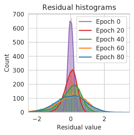
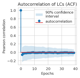
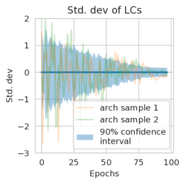
Finally, we consider three different noise models as described in Section 3. Recall that we create a new dataset of predicted $\bm{\epsilon}_{i}$ values, which we call residuals, by subtracting the reconstructed mean learning curves from the real learning curves in $\mathcal{D}_{\text{train}}$. That is, $\hat{\bm{\epsilon}}_{i}=\bm{y}_{i}-(d_{k}\circ c_{k})\left(\bm{y}_{i}\right)$ is the residual for the $i$th learning curve. Our three noise models are based on two different assumptions: (1) the noise distribution is the same for all architectures, and (2) for each architecture, the noise in a small window of epochs are iid. Now we evaluate these assumptions. In Figure 6 (left), we plot the residuals from the NAS-Bench-301 training set at five different epochs, showing that the distributions are roughly Gaussian, across all architectures. Recall that noise model (i) is a simple standard deviation statistic computed for each epoch independently, across all architectures. In Figure 6 (middle), we plot the autocorrelation function (ACF) averaged over all training learning curves on NAS-Bench-301. We see that there is very little autocorrelation in the learning curves, which justifies the use of the first noise model. Recall that our second noise model uses Gaussian kernel density estimation (GKDE) [58] across all learning curves. This is essentially the same as the first noise model but with the ability to capture the small amount of autocorrelation present. Finally, recall that our our third noise model does not assume that the residual distribution is similar across all architectures. Instead, it estimates the standard deviation for each epoch using a sliding window of size 10 across the epochs for each architecture. See Figure 6 (right) for the 90% confidence intervals of the residuals at each epoch on NAS-Bench-301. Although the sliding window noise model has the benefit of capturing different distributions for different architectures, we see that the standard deviation steadily decreases as the epoch number increases, meaning that the noise in a small window of epochs are not perfectly iid.

In Table 3, we run a full ablation study by testing all eighteen combinations of {SVD, VAE}, {LGB, XGB, MLP}, and {GKDE, STD, window} for NAS-Bench-111 and NAS-Bench-311. Recall that, as explained in Section 3, the first four metrics evaluate only the prediction of the mean learning curves using a held-out test set, so the noise model has no effect on the first four metrics (average $R^{2}$, final $R^{2}$, average KT, and final KT). For the final two metrics (average KL and final KL), we use a test set of learning curves consisting of five seeds of architectures, so that we can estimate the KL divergence between the real learning curve distribution and the predicted distribution. Note that none of the NAS-Bench-NLP architectures were trained more than once, so we are unable to test the noise models for NAS-Bench-NLP11. Across NAS-Bench-111, NAS-Bench-311, and NAS-Bench-NLP11, we see that SVD-LGB performs substantially better than all of the other options for the model.

Figure 6: A plot of the residuals across all architectures for five different epochs (left). We see that the distributions are roughly Gaussian. A plot of the autocorrelation function (ACF) averaged over all training learning curves (middle). We see that there is only a small amount of autocorrelation. A plot of the 90% confidence intervals of the residuals at each epoch (right). All plots use the NAS-Bench-301 learning curve training set.

Table 3: Evaluation of the surrogate benchmarks on test sets, with all combinations of models. For NAS-Bench-111 and NAS-Bench-NLP11, we use architecture accuracies as additional features to improve performance. As explained in Section C, no architectures in the NAS-Bench-NLP dataset were trained more than once, so we do not compute KL divergence for NAS-Bench-NLP11.

Benchmark	Avg. $R^{2}$	Final $R^{2}$	Avg. KT	Final KT	Avg. KL	Final KL
NAS-Bench-111
SVD-LGB-GKDE	0.630	0.853	0.611	0.794	1.641	0.516
SVD-LGB-STD	0.630	0.853	0.611	0.794	2.768	0.383
SVD-LGB-window	0.630	0.853	0.611	0.794	24.402	3.303
SVD-XGB-GKDE	0.329	0.378	0.408	0.429	2.743	0.580
SVD-XGB-STD	0.329	0.378	0.408	0.429	4.867	0.503
SVD-XGB-window	0.329	0.378	0.408	0.429	38.457	16.172
SVD-MLP-GKDE	0.195	0.065	0.330	0.290	4.599	0.762
SVD-MLP-STD	0.195	0.065	0.330	0.290	8.417	0.848
SVD-MLP-window	0.195	0.065	0.330	0.290	82.180	15.711
VAE-LGB-GKDE	0.267	0.218	0.462	0.617	3.788	0.829
VAE-LGB-STD	0.267	0.218	0.462	0.617	6.866	0.972
VAE-LGB-window	0.267	0.218	0.462	0.617	53.866	19.820
VAE-XGB-GKDE	0.311	0.272	0.453	0.559	3.828	0.828
VAE-XGB-STD	0.311	0.272	0.453	0.559	6.940	0.969
VAE-XGB-window	0.311	0.272	0.453	0.559	55.654	19.614
VAE-MLP-GKDE	0.218	0.007	0.386	0.369	4.583	0.844
VAE-MLP-STD	0.218	0.007	0.386	0.369	8.386	1.001
VAE-MLP-window	0.218	0.007	0.386	0.369	83.481	19.091
NAS-Bench-311
SVD-LGB-GKDE	0.779	0.800	0.728	0.788	0.503	0.548
SVD-LGB-STD	0.779	0.800	0.728	0.788	0.919	1.036
SVD-LGB-window	0.779	0.800	0.728	0.788	1.566	4.083
SVD-XGB-GKDE	0.522	0.546	0.607	0.654	1.783	3.272
SVD-XGB-STD	0.522	0.546	0.607	0.654	3.271	5.958
SVD-XGB-window	0.522	0.546	0.607	0.654	5.282	19.432
SVD-MLP-GKDE	0.564	0.549	0.573	0.603	15.727	29.057
SVD-MLP-STD	0.564	0.549	0.573	0.603	28.833	52.515
SVD-MLP-window	0.564	0.549	0.573	0.603	45.071	167.140
VAE-LGB-GKDE	0.431	0.447	0.568	0.616	5.995	13.486
VAE-LGB-STD	0.431	0.447	0.568	0.616	11.015	24.836
VAE-LGB-window	0.431	0.447	0.568	0.616	17.510	79.773
VAE-XGB-GKDE	0.397	0.427	0.577	0.624	6.520	16.739
VAE-XGB-STD	0.397	0.427	0.577	0.624	11.978	30.368
VAE-XGB-window	0.397	0.427	0.577	0.624	18.883	97.485
VAE-MLP-GKDE	0.509	0.520	0.584	0.619	13.545	33.851
VAE-MLP-STD	0.509	0.520	0.584	0.619	24.770	61.455
VAE-MLP-window	0.509	0.520	0.584	0.619	38.593	196.246
NAS-Bench-NLP11
SVD-LGB	0.906	0.882	0.862	0.820	-	-
SVD-XGB	0.849	0.865	0.786	0.735	-	-
SVD-MLP	0.120	0.108	0.292	0.275	-	-
VAE-LGB	0.789	0.795	0.802	0.747	-	-
VAE-XGB	0.826	0.838	0.797	0.739	-	-
VAE-MLP	0.150	0.160	0.315	0.300	-	-

Surrogate training details.

Finally, we give more details for the surrogate training. For NAS-Bench-111, as discussed in Section 3, we created a new set of trained architectures with the full learning curve information. We kept the training pipeline nearly the same as in the orginal NAS-Bench-101 repository. However, instead of the TPU v2 acceleator as in the original work, we used an RTX 3070. We needed to change the batch size from 256 to 200 to account for this hardware change, which we found had a negligible affect on the final accuracy. We trained 1101 new architectures and used this new set as the new “ground-truth” when training and evaluating NAS-Bench-111. As explained in Section 3, the accuracies from the original NAS-Bench-101 benchmark were used as features to improve the performance of our surrogate, but not used as ground truth. In Table 4, we show that the KT values for NAS-Bench-111 are roughly equivalent to those achieved by a 1-seed tabular benchmark.

Table 4: NAS-Bench-111 rank correlations computed on a separate test set with architectures trained for two different random seeds each. This allows the comparison with the rank correlation of an independent set of ground truth architectures. We find that the NAS-Bench-111 mean model is on par with the ground truth.

Benchmark	Avg. $R^{2}$	Final $R^{2}$	Avg. KT	Final KT
NAS-Bench-111	0.557	0.541	0.660	0.860
Ground truth (1 seed)	0.593	0.920	0.619	0.873

For NAS-Bench-311, training was straightforward. We used the original NAS-Bench-301 dataset, which already achieves good coverage [60], and we did not use any additional features. In Table 5, we show that the mean model in NAS-Bench-311 achieves higher rank correlation even than a set of learning curves averaged over four random seeds, by using a separate test set from the NAS-Bench-301 dataset which evaluates 500 architectures with 5 seeds each.

Table 5: NAS-Bench-311 rank correlations computed on a separate test set with architectures trained for five different random seeds each. This allows the comparison with sets of learning curves averaged over multiple seeds. We find that the NAS-Bench-311 mean model performs better than a 4-seed mean.

Benchmark	Avg. $R^{2}$	Final $R^{2}$	Avg. KT	Final KT
NAS-Bench-311	0.731	0.845	0.637	0.718
Ground truth (1 seed)	0.534	0.782	0.508	0.641
Ground truth (mean of 2 seeds)	0.651	0.835	0.555	0.683
Ground truth (mean of 3 seeds)	0.690	0.859	0.579	0.704
Ground truth (mean of 4 seeds)	0.710	0.870	0.592	0.712

For NAS-Bench-NLP11, as described earlier, it is challenging to create an accurate surrogate benchmark because there are only $14\,322$ evaluated architectures for a search space of total size $10^{53}$. Therefore, we used two techniques to improve performance. First, we used a subset of the search space, restricting the architectures to a maximum of 12 nodes (reducing the size to $10^{22}$), and we added the validation accuracies from the first three epochs of training each architecture, as features. These two techniques were shown to substantially improve the performance of NAS-Bench-NLP11, as shown in Table 2. On an RTX 3070, training architectures from NAS-Bench-NLP takes about 90 seconds per epoch. Although adding in the first three epochs substantially improves the accuracy of our surrogate benchmark, it comes at the cost of query time. While NAS-Bench-111 and NAS-Bench-311 take under one second to query, a query to NAS-Bench-NLP11 now requires training an architecture for three epochs. Note that this is still a $15\times$ speedup over performing NAS directly without a surrogate benchmark.

We also create NAS-Bench-211 to further evaluate our surrogate creation technique (since NAS-Bench-201 already has complete learning curves). We train the surrogate on 90% of architectures from NAS-Bench-201 (14 062 architectures) and test on the remaining 10%. SVD-LGB-window achieves the best performance. The rank correlation values are on par with a 1-seed tabular benchmark (see Table 6).

Table 6: NAS-Bench-211 rank correlations computed on a test set with architectures trained for three different random seeds each. This allows the comparison with sets of learning curves averaged over multiple seeds. We find that the NAS-Bench-211 mean model performs on par with 1-seed ground truth.

Benchmark	Avg. $R^{2}$	Final $R^{2}$	Avg. KT	Final KT
NAS-Bench-211	0.893	0.958	0.701	0.842
Ground truth (1 seed)	0.866	0.999	0.646	0.916
Ground truth (mean of 2 seeds)	0.900	0.999	0.679	0.926

Appendix D Details from Section 5 (Experiments)

In this section, we give more details from Section 5, and we present more experiments.

Our work uses existing NAS Benchmarks. In Table 7, we report the licenses for each one.

Table 7: Licenses for the datasets that we use.

Dataset	License	URL
NAS-Bench-101	Apache 2.0	https://github.com/google-research/nasbench
NAS-Bench-201	MIT	https://github.com/D-X-Y/NAS-Bench-201
NAS-Bench-301	Apache 2.0	https://github.com/automl/nasbench301
NAS-Bench-NLP	None	https://github.com/fmsnew/nas-bench-nlp-release

D.1 LCE Results

Next, we give the LCE results for four search spaces, which is an extension of the results from Figure 4. That is, we test the improvement of three different single-fidelity algorithms when used with our LCE framework from Section 4, using WPM or SVR as the LCE techniques. We see that across all search spaces, for each single-fidelity algorithm, WPM and SVR both give improvements over the original algorithm, and SVR tends to give the larger improvement compared to WPM. In Figures 5 and 7, an earlier version of the NAS-Bench-NLP11 noise model was used. We also added slight clipping for NAS-Bench-111 and -311 to reduce the number of spike anomalies as described in Section 3.3.

Figure 7: LCE Framework applied to single-fidelity algorithms on NAS-Bench-111, NAS-Bench-311, NAS-Bench-NLP11, and NAS-Bench-201.

D.2 Ablation study.

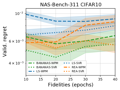
We evaluate the effect of different fidelities on NAS-Bench-311. In Figure 8, we plot the validation regret of the SVR and WPM-based algorithms after $2\times 10^{6}$ seconds, varying the initial fidelity (epoch) from which the learning curve is extracted, from 10 to 40. That is, the leftmost points run LCE by extrapolating from epoch 10 to epoch 100, and the rightmost points run LCE by extrapolating from epoch 40 to epoch 100. Note that there is a tradeoff between time saved (from only evaluating to 10 epochs vs 40) and accuracy of LCE (extrapolating from 10 epochs is more challenging than from 40 epochs). We see that overall, epoch 20 performs the best. Notably, BANANAS-SVR and REA-SVR (two of the best-performing algorithms across all search spaces) achieve top performance at epoch 20.

Figure 8: Different fidelities and their effect on NAS performance on NAS-Bench-311. The wall-clock time [s] is set to 2e6. The result are reported across 30 seeds.

D.3 NAS algorithm descriptions and details

We give a description and implementation details for each NAS algorithm from Section 5. Note that all algorithms were implemented in NASLib [56], keeping the implementation as close as possibe to the original implementation.

• Random search. Random search is a simple baseline which draws architectures at random and then returns the architecture with the lowest validation error. Note that multiple papers have shown that random search is competitive with other NAS algorithms [34, 57].

• Local search. Another baseline, local search has been shown to perform surprisingly well [68, 48], even on the DARTS search space [60]. It works by iteratively evaluating all architectures in the neighborhood of the current best architecture found so far. The neighborhood is defined as the set of architectures which differ by one operation or edge. We used the implementation from NASLib [56]. Notably, this is slightly different from the White et al. [68] implementation which may explain the worse performance on NAS-Bench-311.

• BANANAS. This algorithm [67] is based on Bayesian optimization using an ensemble of three MLPs as the model. We use the code directly from the original repository. We set the encoding to the adjacency matrix encoding instead of the path encoding. A predictor (trained on all architectures evaluated so far) chooses $k$ architectures which are then evaluated. In our experiments, the candidate pool is created by mutating the top four architectures ten times each (two times for each of the edit distance from one to five), and we set $k=20$.

• Regularized evolution. This algorithm [53] is based on evolution. It consists of iteratively mutating the best architectures out of a sample of all architectures evaluated so far. A mutation is defined as randomly changing one operation or edge. We used the NAS-Bench-101 [76] implementation, changing the population size from 50 to 20.

• Hyperband. This algorithm [35] is based on random search with successive halving. It is based on successive halving, in which architectures are iteratively trained at a low fidelity, and then only the best-performing architectures are trained for longer in the next iteration, until the maximum number of epochs is reached. Hyperband performs multiple rounds of successive halving at different initial fidelities. We use the hpbandster implementation, adapted to NASLib [56].

• Bayesian optimization Hyperband. This algorithm [14] is based on combining Hyperband with Bayesian optimization. It starts the same way as Hyperband, but in the later rounds, for each fidelity a KDE model is trained using the trained architectures from previous rounds. Then the best architectures are chosen using Bayesian optimization with the model. We use the hpbandster implementation, adapted to NASLib [56].

References

- [1] Bowen Baker, Otkrist Gupta, Ramesh Raskar, and Nikhil Naik. Accelerating neural architecture search using performance prediction. In ICLR Workshop, 2018.
- [2] Gabriel Bender, Pieter-Jan Kindermans, Barret Zoph, Vijay Vasudevan, and Quoc Le. Understanding and simplifying one-shot architecture search. In ICML, 2018.
- [3] James S Bergstra, Rémi Bardenet, Yoshua Bengio, and Balázs Kégl. Algorithms for hyper-parameter optimization. In NeurIPS, 2011.
- [4] Akshay Chandrashekaran and Ian R Lane. Speeding up hyper-parameter optimization by extrapolation of learning curves using previous builds. In ECML-PKDD, 2017.
- [5] Tianqi Chen and Carlos Guestrin. Xgboost: A scalable tree boosting system. In Proceedings of the 22nd acm sigkdd international conference on knowledge discovery and data mining, pages 785–794, 2016.
- [6] Xiangning Chen, Ruochen Wang, Minhao Cheng, Xiaocheng Tang, and Cho-Jui Hsieh. Drnas: Dirichlet neural architecture search. In ICLR, 2021.
- [7] Patryk Chrabaszcz, Ilya Loshchilov, and Frank Hutter. A downsampled variant of imagenet as an alternative to the cifar datasets. In arXiv:1707.08819, 2017.
- [8] Tobias Domhan, Jost Tobias Springenberg, and Frank Hutter. Speeding up automatic hyperparameter optimization of deep neural networks by extrapolation of learning curves. In IJCAI, 2015.
- [9] Xuanyi Dong, Lu Liu, Katarzyna Musial, and Bogdan Gabrys. Nats-bench: Benchmarking nas algorithms for architecture topology and size. In PAMI, 2021.
- [10] Xuanyi Dong and Yi Yang. Searching for a robust neural architecture in four gpu hours. In CVPR, 2019.
- [11] Xuanyi Dong and Yi Yang. Nas-bench-201: Extending the scope of reproducible neural architecture search. In ICLR, 2020.
- [12] Katharina Eggensperger, Frank Hutter, Holger Hoos, and Kevin Leyton-Brown. Efficient benchmarking of hyperparameter optimizers via surrogates. In AAAI, 2015.
- [13] Thomas Elsken, Jan Hendrik Metzen, and Frank Hutter. Neural architecture search: A survey. In JMLR, 2019.
- [14] Stefan Falkner, Aaron Klein, and Frank Hutter. Bohb: Robust and efficient hyperparameter optimization at scale. In ICML, 2018.
- [15] Matilde Gargiani, Aaron Klein, Stefan Falkner, and Frank Hutter. Probabilistic rollouts for learning curve extrapolation across hyperparameter settings. arXiv preprint arXiv:1910.04522, 2019.
- [16] Gene Golub and William Kahan. Calculating the singular values and pseudo-inverse of a matrix. Journal of the Society for Industrial and Applied Mathematics, Series B: Numerical Analysis, 2(2):205–224, 1965.
- [17] Karen Hao. Training a single ai model can emit as much carbon as five cars in their lifetimes. MIT Technology Review, 2019.
- [18] Hanzhang Hu, John Langford, Rich Caruana, Saurajit Mukherjee, Eric Horvitz, and Debadeepta Dey. Efficient forward architecture search. In NeurIPS, 2019.
- [19] Yimin Huang, Yujun Li, Hanrong Ye, Zhenguo Li, and Zhihua Zhang. An asymptotically optimal multi-armed bandit algorithm and hyperparameter optimization. arXiv preprint arXiv:2007.05670, 2020.
- [20] Kirthevasan Kandasamy, Gautam Dasarathy, Junier B. Oliva, Jeff Schneider, and Barnabas Poczos. Multi-fidelity gaussian process bandit optimisation. In NeurIPS, 2016.
- [21] Kirthevasan Kandasamy, Gautam Dasarathy, Jeff Schneider, and Barnabas Poczos. Multi-fidelity bayesian optimisation with continuous approximations. In JMLR, 2017.
- [22] Kirthevasan Kandasamy, Willie Neiswanger, Jeff Schneider, Barnabas Poczos, and Eric P Xing. Neural architecture search with bayesian optimisation and optimal transport. In NeurIPS, 2018.
- [23] Guolin Ke, Qi Meng, Thomas Finley, Taifeng Wang, Wei Chen, Weidong Ma, Qiwei Ye, and Tie-Yan Liu. Lightgbm: A highly efficient gradient boosting decision tree. In NeurIPS, 2017.
- [24] Maurice G Kendall. A new measure of rank correlation. Biometrika, 30(1/2):81–93, 1938.
- [25] Diederik P Kingma and Max Welling. Auto-encoding variational bayes. In ICLR, 2014.
- [26] Hiroaki Kitano. Designing neural networks using genetic algorithms with graph generation system. Complex systems, 4(4):461–476, 1990.
- [27] Aaron Klein, Stefan Falkner, Simon Bartels, Philipp Hennig, and Frank Hutter. Fast Bayesian Optimization of Machine Learning Hyperparameters on Large Datasets. In AISTATS, 2017.
- [28] Aaron Klein, Stefan Falkner, Jost Tobias Springenberg, and Frank Hutter. Learning curve prediction with bayesian neural networks. In ICLR, 2017.
- [29] Aaron Klein, Louis Tiao, Thibaut Lienart, Cedric Archambeau, and Matthias Seeger. Model-based asynchronous hyperparameter and neural architecture search. arXiv preprint arXiv:2003.10865, 2020.
- [30] Nikita Klyuchnikov, Ilya Trofimov, Ekaterina Artemova, Mikhail Salnikov, Maxim Fedorov, and Evgeny Burnaev. Nas-bench-nlp: neural architecture search benchmark for natural language processing. arXiv preprint arXiv:2006.07116, 2020.
- [31] Alex Krizhevsky. Learning multiple layers of features from tiny images. Technical report, University of Toronto, 2009.
- [32] Liam Li, Kevin Jamieson, Afshin Rostamizadeh, Ekaterina Gonina, Moritz Hardt, Benjamin Recht, and Ameet Talwalkar. A system for massively parallel hyperparameter tuning. In MLSys Conference, 2020.
- [33] Liam Li, Mikhail Khodak, Maria-Florina Balcan, and Ameet Talwalkar. Geometry-aware gradient algorithms for neural architecture search. In Proceedings of the International Conference on Learning Representations (ICLR), 2021.
- [34] Liam Li and Ameet Talwalkar. Random search and reproducibility for neural architecture search. In UAI, 2019.
- [35] Lisha Li, Kevin Jamieson, Giulia DeSalvo, Afshin Rostamizadeh, and Ameet Talwalkar. Hyperband: A novel bandit-based approach to hyperparameter optimization. In JMLR, 2018.
- [36] Marius Lindauer and Frank Hutter. Best practices for scientific research on neural architecture search. In JMLR, 2020.
- [37] Chenxi Liu, Barret Zoph, Maxim Neumann, Jonathon Shlens, Wei Hua, Li-Jia Li, Li Fei-Fei, Alan Yuille, Jonathan Huang, and Kevin Murphy. Progressive neural architecture search. In ECCV, 2018.
- [38] Hanxiao Liu, Karen Simonyan, and Yiming Yang. Darts: Differentiable architecture search. In ICLR, 2019.
- [39] Renqian Luo, Xu Tan, Rui Wang, Tao Qin, Enhong Chen, and Tie-Yan Liu. Semi-supervised neural architecture search. In NeurIPS, 2020.
- [40] Neeratyoy Mallik and Noor Awad. Dehb: Evolutionary hyperband for scalable, robust and efficient hyperparameter optimization. In IJCAI, 2021.
- [41] Abhinav Mehrotra, Alberto Gil C. P. Ramos, Sourav Bhattacharya, Łukasz Dudziak, Ravichander Vipperla, Thomas Chau, Mohamed S Abdelfattah, Samin Ishtiaq, and Nicholas Donald Lane. Nas-bench-asr: Reproducible neural architecture search for speech recognition. In ICLR, 2021.
- [42] Tomáš Mikolov, Martin Karafiát, Lukáš Burget, Jan Černockỳ, and Sanjeev Khudanpur. Recurrent neural network based language model. In Annual conference of the international speech communication association, 2010.
- [43] Geoffrey F Miller, Peter M Todd, and Shailesh U Hegde. Designing neural networks using genetic algorithms. In ICGA, volume 89, pages 379–384, 1989.
- [44] Renato Negrinho and Geoff Gordon. Deeparchitect: Automatically designing and training deep architectures. arXiv preprint arXiv:1704.08792, 2017.
- [45] Vu Nguyen, Sebastian Schulze, and Michael Osborne. Bayesian optimization for iterative learning. In NeurIPS, 2020.
- [46] Xuefei Ning, Wenshuo Li, Zixuan Zhou, Tianchen Zhao, Yin Zheng, Shuang Liang, Huazhong Yang, and Yu Wang. A surgery of the neural architecture evaluators. arXiv preprint arXiv:2008.03064, 2020.
- [47] Changyong Oh, Jakub M Tomczak, Efstratios Gavves, and Max Welling. Combinatorial bayesian optimization using the graph cartesian product. arXiv preprint arXiv:1902.00448, 2019.
- [48] T Den Ottelander, Arkadiy Dushatskiy, Marco Virgolin, and Peter AN Bosman. Local search is a remarkably strong baseline for neural architecture search. In International Conference on Evolutionary Multi-Criterion Optimization, 2021.
- [49] Adam Paszke, Sam Gross, Francisco Massa, Adam Lerer, James Bradbury, Gregory Chanan, Trevor Killeen, Zeming Lin, Natalia Gimelshein, Luca Antiga, et al. Pytorch: An imperative style, high-performance deep learning library. In Proceedings of the Annual Conference on Neural Information Processing Systems (NeurIPS), 2019.
- [50] David Patterson, Joseph Gonzalez, Quoc Le, Chen Liang, Lluis-Miquel Munguia, Daniel Rothchild, David So, Maud Texier, and Jeff Dean. Carbon emissions and large neural network training. arXiv preprint arXiv:2104.10350, 2021.
- [51] Houwen Peng, Hao Du, Hongyuan Yu, Qi Li, Jing Liao, and Jianlong Fu. Cream of the crop: Distilling prioritized paths for one-shot neural architecture search. In NeurIPS, 2020.
- [52] Hieu Pham, Melody Y Guan, Barret Zoph, Quoc V Le, and Jeff Dean. Efficient neural architecture search via parameter sharing. In ICML, 2018.
- [53] Esteban Real, Alok Aggarwal, Yanping Huang, and Quoc V Le. Regularized evolution for image classifier architecture search. In AAAI, 2019.
- [54] Binxin Ru, Clare Lyle, Lisa Schut, Mark van der Wilk, and Yarin Gal. Revisiting the train loss: an efficient performance estimator for neural architecture search. arXiv preprint arXiv:2006.04492, 2020.
- [55] Binxin Ru, Xingchen Wan, Xiaowen Dong, and Michael Osborne. Neural architecture search using bayesian optimisation with weisfeiler-lehman kernel. In ICLR, 2021.
- [56] Michael Ruchte, Arber Zela, Julien Siems, Josif Grabocka, and Frank Hutter. Naslib: a modular and flexible neural architecture search library, 2020.
- [57] Christian Sciuto, Kaicheng Yu, Martin Jaggi, Claudiu Musat, and Mathieu Salzmann. Evaluating the search phase of neural architecture search. In ICLR, 2020.
- [58] David W Scott. Multivariate density estimation: theory, practice, and visualization. John Wiley & Sons, 2015.
- [59] Han Shi, Renjie Pi, Hang Xu, Zhenguo Li, James Kwok, and Tong Zhang. Bridging the gap between sample-based and one-shot neural architecture search with bonas. In NeurIPS, 2020.
- [60] Julien Siems, Lucas Zimmer, Arber Zela, Jovita Lukasik, Margret Keuper, and Frank Hutter. Nas-bench-301 and the case for surrogate benchmarks for neural architecture search. arXiv preprint arXiv:2008.09777, 2020.
- [61] Julien Siems, Lucas Zimmer, Arber Zela, Jovita Lukasik, Margret Keuper, and Frank Hutter. Nas-bench-301 and the case for surrogate benchmarks for neural architecture search: Openreview response, 2021.
- [62] Kenneth O Stanley and Risto Miikkulainen. Evolving neural networks through augmenting topologies. Evolutionary computation, 10(2):99–127, 2002.
- [63] Kevin Swersky, Jasper Snoek, and Ryan Prescott Adams. Freeze-thaw bayesian optimization. arXiv preprint arXiv:1406.3896, 2014.
- [64] Chen Wei, Chuang Niu, Yiping Tang, and Jimin Liang. Npenas: Neural predictor guided evolution for neural architecture search. arXiv preprint arXiv:2003.12857, 2020.
- [65] Wei Wen, Hanxiao Liu, Hai Li, Yiran Chen, Gabriel Bender, and Pieter-Jan Kindermans. Neural predictor for neural architecture search. In ECCV, 2020.
- [66] Colin White, Willie Neiswanger, Sam Nolen, and Yash Savani. A study on encodings for neural architecture search. In NeurIPS, 2020.
- [67] Colin White, Willie Neiswanger, and Yash Savani. Bananas: Bayesian optimization with neural architectures for neural architecture search. In AAAI, 2021.
- [68] Colin White, Sam Nolen, and Yash Savani. Local search is state of the art for nas benchmarks. In UAI, 2021.
- [69] Colin White, Arber Zela, Binxin Ru, Yang Liu, and Frank Hutter. How powerful are performance predictors in neural architecture search? arXiv preprint arXiv:2104.01177, 2021.
- [70] Sewall Wright. Correlation and causation. Journal of Agricultural Research, 20:557–580, 1921.
- [71] Lingxi Xie, Xin Chen, Kaifeng Bi, Longhui Wei, Yuhui Xu, Zhengsu Chen, Lanfei Wang, An Xiao, Jianlong Chang, Xiaopeng Zhang, et al. Weight-sharing neural architecture search: A battle to shrink the optimization gap. arXiv preprint arXiv:2008.01475, 2020.
- [72] Yuhui Xu, Lingxi Xie, Xiaopeng Zhang, Xin Chen, Guo-Jun Qi, Qi Tian, and Hongkai Xiong. Pc-darts: Partial channel connections for memory-efficient architecture search. In ICLR, 2019.
- [73] Shen Yan, Kaiqiang Song, Fei Liu, and Mi Zhang. Cate: Computation-aware neural architecture encoding with transformers. In ICML, 2021.
- [74] Shen Yan, Yu Zheng, Wei Ao, Xiao Zeng, and Mi Zhang. Does unsupervised architecture representation learning help neural architecture search? In NeurIPS, 2020.
- [75] Antoine Yang, Pedro M Esperança, and Fabio M Carlucci. Nas evaluation is frustratingly hard. In ICLR, 2020.
- [76] Chris Ying, Aaron Klein, Esteban Real, Eric Christiansen, Kevin Murphy, and Frank Hutter. Nas-bench-101: Towards reproducible neural architecture search. In ICML, 2019.
- [77] Shan You, Tao Huang, Mingmin Yang, Fei Wang, Chen Qian, and Changshui Zhang. Greedynas: Towards fast one-shot nas with greedy supernet. In CVPR, 2020.
- [78] Kaicheng Yu, Rene Ranftl, and Mathieu Salzmann. Landmark regularization: Ranking guided super-net training in neural architecture search. In CVPR, 2021.
- [79] Arber Zela, Thomas Elsken, Tonmoy Saikia, Yassine Marrakchi, Thomas Brox, and Frank Hutter. Understanding and robustifying differentiable architecture search. In ICLR, 2020.
- [80] Arber Zela, Julien Siems, and Frank Hutter. Nas-bench-1shot1: Benchmarking and dissecting one-shot neural architecture search. In ICLR, 2020.
- [81] Yuge Zhang, Zejun Lin, Junyang Jiang, Quanlu Zhang, Yujing Wang, Hui Xue, Chen Zhang, and Yaming Yang. Deeper insights into weight sharing in neural architecture search. arXiv preprint arXiv:2001.01431, 2020.
- [82] Barret Zoph and Quoc V. Le. Neural architecture search with reinforcement learning. In ICLR, 2017.
- [83] Barret Zoph, Vijay Vasudevan, Jonathon Shlens, and Quoc V Le. Learning transferable architectures for scalable image recognition. In CVPR, 2018.