Arnold diffusion and Nekhoroshev theory

Abstract

Starting with Arnold’s pioneering work [2], the term “Arnold diffusion” has been used to describe the slow diffusion taking place in the space of the actions in Hamiltonian nonlinear dynamical systems with three or more degrees of freedom. The present text is an elaborated transcript of the introductory course given in the Milano I-CELMECH school on the topic of Arnold diffusion and its relation to Nekhoroshev theory. The course introduces basic concepts related to our current understanding of the mechanisms leading to Arnold diffusion. Emphasis is placed upon the identification of those invariant objects in phase space which drive chaotic diffusion, such as the stable and unstable manifolds emanating from (partially) hyperbolic invariant objects. Besides a qualitative understanding of the diffusion mechanisms, a precise quantification of the speed of Arnold diffusion can be achieved by methods based on canonical perturbation theory, i.e. by the construction of a suitable normal form at optimal order. As an example of such methods, we discuss the (quasi-)stationary-phase approximation for the selection of remainder terms acting as driving terms for the diffusion. Finally, we discuss the efficiency of such methods through numerical examples in which the optimal normal form is determined by a computer-algebraic implementation of a normalization algorithm.

1 Introduction

In some introductory texts (see, for example, [58][46][17]), the topic of Arnold diffusion is introduced by a simplified topological argument, related to a difference between the cases of invariant tori in Hamiltonian systems with $n=2$ and with $n\geq 3$ degrees of freedom. Consider a $n-$degrees of freedom Hamiltonian system $H(q,p)$, $q\in\mathbb{R}^{n}$, $p\in\mathbb{R}^{n}$, whose phase space contains a large measure of $n-$dimensional Kolmogorov - Arnold - Moser (KAM) tori ([43, 1, 51]). Any orbit $(q(t),p(t))$ with initial conditions $(q_{0},p_{0})$ on a KAM torus remains forever confined to the torus. Any orbit with initial conditions $(q_{0},p_{0})$ belonging to the complement, in phase space, with respect to the set of all KAM tori, remains confined to the $(2n-1)$-dimensional manifold defined by the orbit’s constant energy value ${\cal M}_{E}:=\{(q,p)\in\mathbb{R}^{2n}:H(q,p)=E=H(q_{0},p_{0})\}$. Take first $n=2$. Thus, $\dim\left({\cal M}_{E}\right)=3$. Suppose there is a KAM torus ${\cal T}$ embedded in the same energy manifold. We have $\dim\left({\cal T}\right)=2$. Since the torus’s dimension differs just by one from the dimension of the energy manifold, ${\cal T}$ divides ${\cal M}_{E}$ into two parts, which can be called the ‘interior’ and the ‘exterior’ of the torus. Furthermore, since $H(q,p)$ is autonomous, there can be no trajectory going from the interior to the exterior of the torus; such a trajectory would necessarily have to cross transversally the torus at a point $(q(t_{c}),p(t_{c}))\in{\cal T}$ at some time $t_{c}$, but this is impossible since the flow on the torus is invariant, i.e., the initial condition $q=q(t_{c}),p=p(t_{c})$ would lead necessarily to a trajectory confined on the torus. We roughly refer to this as the ‘dividing property’ of KAM tori in systems with $n=2$ degrees of freedom. On the other hand, there is no dividing property of the KAM tori when $n\geq 3$, since, in that case $\dim\left({\cal M}_{E}\right)-\dim\left({\cal T}\right)\geq 2$. For example, when $n=3$ we have $\dim({\cal M})=5$, and $\dim({\cal T})=3$, thus ${\cal T}$ cannot divide ${\cal M}$ into disconnected sets. To visualize this just lower all dimensions in the above examples by one: hence, a circle (dimension 1) divides a plane (dimension 2) to the interior and the exterior of the circle, while a circle embedded in Euclidean space (dimension 3) cannot divide the latter into disconnected sets.

The non-existence of topological barriers when $n\geq 3$ renders a priori possible to have long excursions of the chaotic orbits throughout the whole constant energy manifold. However, two questions become immediately relevant: i) can we prove that the chaotic orbits do really undergo those (topologically allowed) arbitrarily long chaotic excursions? ii) is the timescale involved short enough to make the phenomenon relevant and worth of further study as regards applications in physical systems (including, for the purposes of the present course, systems of interest in celestial mechanics or astrodynamics)?

We refer to question (i) above as the problem of the existence of Arnold diffusion. In the words of Lochak’s influential review [49], it is the problem of demonstrating that “topological transitivity on the energy surface generically takes place”. We refer, instead, to question (ii) as the problem of how to quantitatively estimate the speed of Arnold diffusion. Addressing this question in the context of particular problems encountered in physics and astronomy requires a (partly heuristic) use of computational techniques, as discussed in detail, for example, in a well known review by Chirikov [13]. It is worth mentioning that, after about 60 years of research, only partial answers are available today regarding both questions. In particular, the existence of Arnold diffusion has been rigorously established in various cases of so-called a priori unstable systems (see [11][10][32][22]). Instead, it remains an open problem in the far more difficult case of a priori stable systems (see section 3 for definitions). In the latter case, we avail, however, ample numerical evidence of the global drift of the trajectories within the so-called Arnold’s web of resonances, as visualized in a series of beautiful numerical studies ([44][37][30] [38]; see [45] for a review). In fact, the visualization of the Arnold web in a priori stable systems was made possible by the use of techniques allowing to carefully choose initial conditions along the thin resonance layers in phase space marked by the web of resonances. The Fast Lyapunov Indicator (FLI, [28]) is an example of such technique (see also the lecture by M. Guzzo in the present volume of proceedings).

As emphasized by Lochak [49], a demonstration that the Arnold diffusion really takes place requires establishing the existence of a mechanism of transport for the weakly chaotic orbits within the Arnold web. Arnold’s original example [2] actually describes such a mechanism. This is based on proving the existence of heteroclinic intersections between the stable and unstable manifolds emanating from a set of nearby partially hyperbolic low-dimensional tori arranged in a so-called ‘transition chain’. One initially demonstrates that two nearby tori, of a small distance, say, ${\cal O}(\delta)$, where $\delta$ is a small parameter, exhibit a ‘splitting of the separatrices’ (their stable and unstable manifolds) such that these manifolds develop heteroclinic intersections. Let $\tau_{i}$, $i=1,2,\ldots$ be a sequence of tori, $\tau_{i}$ being neighbor to $\tau_{i-1},\tau_{i+1}$. Assume we know that the unstable manifold emanating from $\tau_{i}$ has a heteroclinic intersection with the stable manifold ending at $\tau_{i+1}$. Then, there is a ‘doubly asymptotic’ orbit which tends to $\tau_{i}$ as $t\rightarrow-\infty$, while it tends to $\tau_{i+1}$ forward in time as $t\rightarrow\infty$. Such orbits can be established for any pair $\tau_{i},\tau_{i+1}$, $i=1,2,...$, but of course they cannot themselves be the orbits of Arnold diffusion, since they never go very far either from $\tau_{i}$ or $\tau_{i+1}$. On the other hand, invoking a so-called ‘shadowing lemma’ (see [20] for a review), one demonstrates that there are true orbits of the system which shadow the whole chain of heteroclinic orbits established in the above way. Thus, these shadowing orbits undergo Arnold diffusion. A quick estimate of the speed of diffusion is obtained as follows: upon completion of one cycle of the transition mechanism, the trajectory has traveled a distance $S={\cal O}(\delta)$ in a time $T_{i,i+1}\approx T_{s}$, which roughly coincides with the time required to cover one homoclinic loop close to the separatrix of the resonance associated with the unstable tori $\tau_{i}$ (see section 2 below). Hence, the local speed of Arnold diffusion is $V_{AD}\approx\delta/T_{s}$, where both parameters $\delta$ and $T_{s}$ depend on the small parameters of the problem under study. Of course, this is an oversimplified estimate. Estimates of practical interest are rather hard to obtain, as explained in the sections to follow. On the other hand, the topic of how to describe itself the one-step transition of the chaotic trajectories far from, and then back to the asymptotic ends of the intersecting manifolds has been developed substantially in recent years, leading to the concept of the so-called ‘scattering map’ (see [19][21]). Applications of the scattering map technique in Celestial Mechanics are discussed, in particular, by [6] (see also [8] and references therein).

Regarding numerical investigations of Arnold diffusion, since this is a slow phenomenon its revelation requires a rather high computing power and the capacity to numerical propagate large sets of trajectories over long integration times. Owing to its complexity, the numerical investigation of the weakly chaotic diffusion has so far been limited to few DOF dynamical systems, including several systems of particular interest for dynamical astronomy (see an extensive, but only indicative, list of references in section 4 of [25]). However, it is unclear whether the notion of Arnold diffusion can be useful for the analysis of the diffusive processes in all those models. On the other hand, there are cases, in particular around normally hyperbolic invariant objects in the restricted three-body problem, where Arnold diffusion has been explicitly demonstrated to apply (see, for example, [52][6] [7][8][27]).

The present tutorial is organized as follows: section 2 presents in some detail the original example discussed in [2], serving to introduce most elements of the conceptual framework for the discussion of Arnold diffusion. Section 3 deals with the case of a priori stable systems and with the connection of Arnold diffusion with Nekhoroshev theory. Finally, Section 4 discusses various semi-analytical approaches to the quantification of the speed of Arnold diffusion.

2 Arnold’s example

The Hamiltonian model presented by Arnold in [2] is

$$H(q,\phi_{1},t,p,J_{1})=\frac{1}{2}p^{2}+\frac{1}{2}J_{1}^{2}+\epsilon\left(\cos q-1\right)\,\left(1+\mu\left(\sin\phi_{1}+\cos t\right)\right)~{},$$ (1)

It is a model of a pendulum (variables $(q,p)$) coupled with a rotator (variables $(\phi_{1},J_{1})$) via the time-dependent term $\epsilon\mu\cos q\cos t$. We will assume $\epsilon>0$ and fixed, while varying $\mu$, with $|\mu|<<\epsilon$. The Hamiltonian can be formally extended to 3DOF autonomous by introducing the angle $\phi_{2}=t$ conjugated to a dummy action $J_{2}$:

$$H\rightarrow H(q,\phi_{1},\phi_{2},p,J_{1},J_{2})=\frac{1}{2}p^{2}+\frac{1}{2}J_{1}^{2}+J_{2}+\epsilon\left(\cos q-1\right)\,\left(1+\mu\left(\sin\phi_{1}+\cos\phi_{2}\right)\right)~{}.$$ (2)

For $\mu=0$, we have $\dot{J_{1}}=\dot{J_{2}}=0$, thus the actions remain invariant along the trajectories. For any values $(J_{1},J_{2})$, the angles $\phi_{1}$, $\phi_{2}$ evolve linearly with frequencies $\omega_{1}=J_{1}$, $\omega_{2}=1$. Thus, changing the value of $J_{1}$, we can obtain any desired frequency ratio $\omega_{1}/\omega_{2}=J_{1}$ (the dummy action $J_{2}$ can be set initially to any value (e.g. $J_{2}(0)=0$) without consequences for the dynamics).

Consider now the case $\mu\neq 0$. For generic trajectories, we obtain $\dot{J}_{1}\neq 0$, $\dot{J}_{2}\neq 0$. However, there is a particular set of initial conditions for which the trajectories preserve the actions:

$$\tau(J_{1},J_{2})=\left\{q=p=0,J_{1}=const,J_{2}=const,(\phi_{1},\phi_{2})\in\mathbb{T}^{2}\right\}~{}~{}.$$ (3)

Taking Hamilton’s equations for the complete system:

$$\dot{q} =p,~{}~{}~{}~{}\dot{p} =-\epsilon\sin q(1+\mu(\sin\phi_{1}+\cos\phi_{2}))$$

$$\dot{\phi_{1}} =J_{1},~{}~{}~{}\dot{J}_{1} =~{}~{}\epsilon\mu(\cos q-1)\cos\phi_{1}$$ (4)

$$\dot{\phi_{2}} =1,~{}~{}~{}\dot{J}_{2} =-\epsilon\mu(\cos q-1)\sin\phi_{2}$$

we immediately find that any initial condition in the set $\tau(J_{1},J_{2})$ leads to $\dot{q}=\dot{p}=0=\dot{J}_{1}=\dot{J}_{2}=0$, while $\dot{\phi}_{1}=J_{1}(t)=const$, $\dot{\phi}_{2}=J_{2}(t)=const$. Thus, $\tau(J_{1},J_{2})$ is invariant under the flow and homeomorphic to the 2D-torus $(\phi_{1},\phi_{2})\in\mathbb{T}^{2}$. We will denote by $\mathcal{T}$ the invariant set formed by the family of all the tori $\tau(J_{1},J_{2})$ $(J_{1},J_{2})\in\mathbb{R}^{2}$.

The invariance of the tori $\tau(J_{1},J_{2})$ crucially relies on having set $(q,p)$ as $(q,p)=(0,0)$. We now wish to explore what will happen if, instead, we choose the initial condition $(q_{0},p_{0})$ close to, but not equal to $(0,0)$. For example, we can set $q_{0}=0,p_{0}\neq 0$, with $|p_{0}|<D$ and $D$ small, and $(J_{1,0},J_{2,0},\phi_{1,0},\phi_{2,0})$ chosen at will. We then want to understand the future evolution, in particular of the actions $J_{1}(t),J_{2}(t)$, as a consequence of choosing initial conditions in the neighborhood of, but not exactly on the torus $\tau(J_{10},J_{20})$. Addressing this question requires the use of a mixture of analytical as well as geometric arguments. Let us summarize some basic ones:

2.1 Existence of KAM tori

We can demonstrate the existence of Kolmogorov-Arnold-Moser (KAM) tori for a Cantor set (of non-zero measure) of initial conditions $p_{0}$ along the line $q=0$. Decomposing the Hamiltonian as:

$$H(q,\phi_{1},\phi_{2},p,J_{1},J_{2})=H_{0}(p,J_{1},J_{2})+\epsilon H_{1}(q,\phi_{1},\phi_{2},p,J_{1},J_{2};\mu)$$ (5)

where $H_{0}={1\over 2}(p^{2}+J_{1}^{2})+J_{2}$, $H_{1}=\epsilon\left(\cos q-1\right)\,\left(1+\mu\left(\sin\phi_{1}+\cos\phi_{2}\right)\right)$, the Hamiltonian $H_{0}$ satisfies the iso-energetic non-degeneracy condition:

$$\det\left(\begin{array}[]{cc}\mbox{Hess}(H_{0})&\nabla_{I}(H_{0})\\ (\nabla_{I}(H_{0}))^{T}&0\end{array}\right)=0$$ (6)

where $\mbox{Hess}(H_{0})$ is the $3\times 3$ Hessian matrix of $H_{0}$ with respect to $I\equiv(p,J_{1},J_{2})$. Thus, the necessary conditions for the Kolmogorov theorem [43] hold, namely:

Theorem (Kolmogorov 1954): there exist positive constants $\epsilon_{0},\gamma,\tau$ such that, for $|\epsilon|<\epsilon_{0}$, and $(p_{0},J_{10})$ such that the frequencies $\omega_{p}=(\partial H_{0}/\partial p)_{p=p_{0}}=p_{0}$, $\omega_{1}=J_{1}$, $\omega_{2}=1$ satisfy the Diophantine condition

$$|k_{p}\omega_{p}+k_{1}\omega_{1}+k_{2}\omega_{2}|>{\gamma\over k^{\tau}}$$ (7)

where $k=|k_{p}|+|k_{1}|+|k_{2}|$, the trajectory with initial conditions $p(0)=p_{0}$, $J_{1}(0)=J_{10})$, $q(0)=0$, $J_{2}(0)=J_{20}\in\mathbb{R}$, as well as $(\phi_{1}(0),\phi_{2}(0))\in\mathbb{T}^{2}$ lies in a three-dimensional torus, where all phase-space co-ordinates evolve quasi-periodically with the frequencies $(\omega_{p},\omega_{1},\omega_{2})$.

The above theorem can be proven by the construction of the so-called Kolmogorov normal form in the neighborhood of the chosen initial conditions. The value of $\gamma$ restricts the measure of initial conditions satisfying the Diophantine condition. By number-theoretical arguments we find $|p_{0}|>D={\cal O}(\gamma)$, hence motions very close to $p_{0}=0$ cannot be quasi-periodic.

2.2 Semi-analytical (‘Melnikov’) approach

In order to deal with non-quasiperiodic motions, very close to the torus $p_{0}=0$, we can try to approximate the evolution of the variables $(\phi_{1},\phi_{2},J_{1},J_{2})$ by a model in which the evolution in the variables $(q(t),p(t))$ is a priori modeled via some ‘near-separatrix’ analytical approximation $(q_{s}(t;\varepsilon_{s}),p_{s}(t;\varepsilon_{s}))$ based on the pendulum model (or, in general, the model of resonance giving rise to a particular form of the separatrix). This strategy is explored heuristically in a well known review on Arnold diffusion by Chirikov [13] and set in a rigorous base in [42]. It is based on the remark that choosing $(q_{0},p_{0})$ very close to the values $(0,0)$ leads to a motion in the variables $(q(t),p(t))$ which can be modeled as a sequence of stochastic alterations between pendulum librations or rotations, each with nearly conserved pendulum energy

$$h_{s}(q,p)=\varepsilon_{s}={1\over 2}p^{2}+\epsilon(\cos q-1)~{}~{}$$ (8)

with $\varepsilon_{s}\approx\varepsilon_{s,0}=0$ (corresponding to the invariant torus $(q,p)=(0,0)$). Figure 1 exemplifies this approach. The figure shows the evolution of the trajectory with initial conditions $q(0)=0$,$\phi_{1}(0)=0$, $\phi_{2}(0)=0$, $p(0)=5{\scriptstyle\times 10}^{[}-5]$, $J_{1}(0)=0.3\sqrt{2}$, $J_{2}=0$, under the complete flow (2), with $\epsilon=0.03$ and $\mu=0.01$.

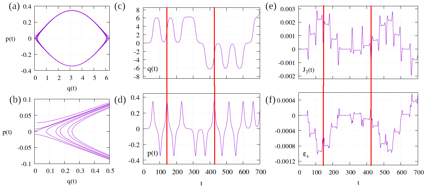
Figure 1: Evolution of the orbit with initial conditions $\phi_{1}(0)=0$, $\phi_{2}(0)=0$, $p(0)=5{\scriptstyle\times 10}^{[}-5]$, $J_{1}(0)=0.3\sqrt{2}$, $J_{2}=1$, under the flow of the Hamiltonian (2) with $\epsilon=0.03$ and $\mu=0.01$: $p(t)$ vs $q(t)$ in panel (a) and (b), $q(t)$ in panel (c),$p(t)$ in panel (d), $J_{1}(t)$ in panel (e), in the time interval $t\in[0,700]$. (f) Evolution of the pendulum energy $\varepsilon_{s}$ for the same orbit. In (a) the angle $q(t)$ is shown modulo $2\pi$. The two red vertical lines in panels (c) to (f) are helping guides to the eye: they indicate two different moments where the trajectory passes from the uppermost point of the separatrix. All jumps in $J_{1}(t)$ occur at these passages.

Since the coupling term between pendulum and the rest of the system has size ${\cal O}(\mu\epsilon)$, with $\mu=0.01$ this term is two orders of magnitude smaller than the $\epsilon\cos q$ term defining the pendulum separatrix. As a consequence, the ‘splitting’ of the separatrix will be quite small. This means that there will be only a small error in approximating the evolution of $(q(t),p(t))$ as if it was governed only by the pendulum Hamiltonian $h_{s}(q,p)$ (Eq.(8)). Figure 1 indicates that this is essentially correct. Denote by $R(+),R(-)$ a pendulum rotation with the Hamiltonian $h_{s}(q,p)$ and with $p>0$ or $p<0$ respectively, and by $L(+),L(-)$ the upper and lower parts (again $p>0$ or $p<0$) of a librational curve in the same Hamiltonian. Then, the evolution of $p(t),q(t)$ in Fig. 1 can be represented as a sequence of segments of pendulum librational or rotational curves. Up to $t=700$ we have

$$R(+),L(-),L(+),L(-),L(+),R(-),R(-),L(+),L(-),L(+),L(-),R(+),R(+),\ldots$$

Denoting by $T_{s,i}$, $i=1,2,\ldots$ the time it takes to accomplish one segment, the times $T_{s,i}$ can be estimated as the times between two successive local extrema in Fig. 1(c). We find that $T_{s,i}$ has value nearly always around $T_{s}\lesssim 100$. Also, using the values $q(t_{i}),p(t_{i})$ at the times $t_{i}$ of the local extrema of the curve $q(t)$, we can compute a sequence of corresponding pendulum energies $\varepsilon_{i}=h_{s}(q(t_{i}),p(t_{i}))$ characteristic of each segment.

Chirikov [13] proposed a model to study the qualitative properties of the mapping $(q(t_{i}),p(t_{i}))\rightarrow(q(t_{i+1}),p(t_{i+1}))$, or, equivalently, $\varepsilon_{i}\rightarrow\varepsilon_{i+1}$, $t_{i}\rightarrow t_{i+1}$, called, by him the whisker mapping (‘whiskers’ meaning the separatrices of the torus $(q,p)=(0,0)$). Figure 1(f) shows the first few transitions in the energy values $\varepsilon_{s}$. In every step, $\varepsilon_{s}(t)$ takes nearly constant value in a ‘plateau’, separated from the next plateau by a rapid oscillation. These oscillations take place mid-way along each homoclinic transition far from and back to the neighborhood ofthe torus $(q,p)=(0,0)$.

We now discuss how to exploit the above empirical information in order to model the evolution in the remaining variables $J_{1}$, $J_{2}$, $\phi_{1}$, $\phi_{2}$ along such homoclinic transitions. The so-called ‘Melnikov approach’ consists essentially of the following approximation: in the interval $t_{i}<t<t_{i+1}$, we will evolve the remaining variables according to the approximate system

$$\dot{\phi_{1}} =J_{1},~{}~{}~{}\dot{J}_{1} =~{}~{}\epsilon\mu(\cos q_{s}(t)-1)\cos\phi_{1}$$ (9)

$$\dot{\phi_{2}} =1,~{}~{}~{}\dot{J}_{2} =-\epsilon\mu(\cos q_{s}(t)-1)\sin\phi_{2}$$

which is the same as the original system but with $q(t),p(t)$ substituted with by the solutions $q_{s}(t),p_{s}(t)$ of the pendulum equations

$$\dot{q}_{s}=p_{s},~{}~{}~{}~{}\dot{p}_{s}=-\epsilon\sin q_{s}$$ (10)

with initial conditions $q_{s}=q(t_{i}),p_{s}=p(t_{i})$.

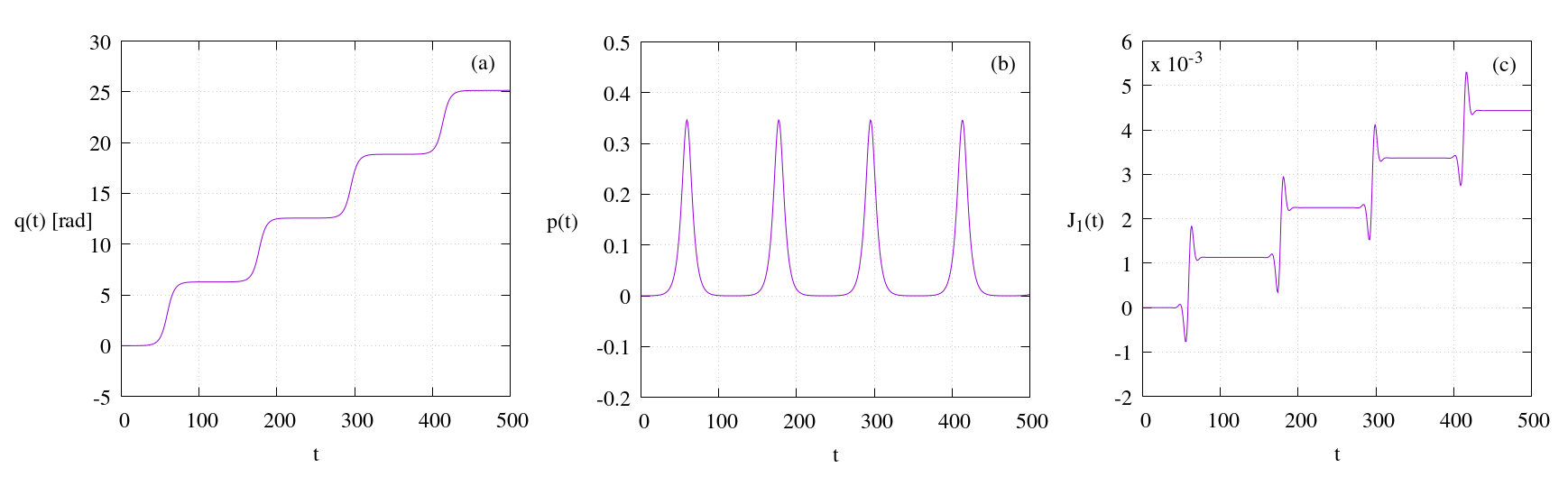
Figure 2: Evolution of the pendulum solution (a) $q_{s}(t)$, (b) $p_{s}(t)$, for the same initial condition as in Fig.1, namely $q_{s}(0)=0$, $p_{s}(0)=5\times 10^{-5}$, but following the pendulum equations (Eqs.(10)). (c) Evolution of the action $J_{1}(t)$ under the equations of the Melnikov approximation (Eqs.(9)). We observe that $J_{1}(t)$ exhibits jumps in time which are qualitatively similar as those of the complete model, shown in panel (e) of Fig.1.

Figure 2 shows the evolution under the approximate equations (10) and (9), starting with the same initial condition as in Fig. 1, which belongs to the upper rotation domain of the pendulum $(q(0)=0,p(0)>0)$. Since we now integrate the exact pendulum equations we obtain a periodic evolution of the angle $q$ completing a circle at the period $T(\varepsilon_{s})$ given by

$$T_{s}(\varepsilon_{s})\simeq\int_{0}^{2\pi}{dq\over\sqrt{2\left(\varepsilon_{s}-\epsilon(\cos q-1)\right)}}={32\over\sqrt{\epsilon}}\ln\left({|\varepsilon_{s}|\over\epsilon}\right)~{}~{}.$$ (11)

However, the action variable $J_{1}(t)$ (Fig.2(c)) undergoes abrupt jumps of size $~{}10^{-3}$ every time when the pendulum variables are mid-way along accomplishing one homoclinic transition.

The jumps in Fig. 2(c) are qualitatively quite similar to the jumps seen in the real orbit (Fig. 1(e)). In fact, the real jumps can be easily modeled by one further simplification: since all along the depicted solution $J_{1}(t)$ undergoes only a small (${\cal O}(10^{-3})$) variation around the initial value $J_{10}=0.3\sqrt{2}$, we can approximate the solution of the angular equation $\dot{\phi_{1}}(t)=J_{1}(t)$ by $\phi_{1}(t)=\phi_{1,0}+J_{10}(t-t_{0})$, where $\phi_{1,0}$ is the value of the angle $\phi_{1}$ at the starting time $t_{0}$ of one homoclinic transition. We also approximate the solution $q_{s}(t)$ by the one holding along the pendulum separatrix:

$$q_{s}(t)\approx 4\arctan\left(e^{\sqrt{\epsilon}(t-t_{0}-T_{s}/2)}\right)~{}~{},$$ (12)

with $T_{s}$ still given by Eq. (11) (this last approximation is not really needed, but makes the computation easier with respect to the pendulum solution for the exact initial conditions given in terms of elliptic functions). As shown in Fig. 3(a), the separatrix solution (12) fits the evolution of $q(t)$ along the first homoclinic transition as obtained numerically by the complete model (2) up to a time $t\approx 80$, where the real orbit starts its second homoclinic transition. Using the above approximations, all quantities in the r.h.s. of the differential equation for $J_{1}$ in the system (9) becomes explicit functions of the time $t$, Then, the approximative solution $J_{1}(t)$ can be obtained by quadratures:

$$J_{1}^{(M)}(t)=J_{1}(0)+\epsilon\mu\int_{0}^{t}\left(\cos(4\arctan(\exp(\sqrt{\epsilon}(t^{\prime}-T_{s}/2))))-1\right)\cos(\phi_{10}+J_{10}t^{\prime})dt^{\prime}$$ (13)

An integral of the form (13) is called a ‘Melnikov integral’. It has the distinguishing feature that the integrand contains trigonometric functions $\cos\phi$, with $\phi=m_{q}q+m_{1}\phi_{1}+m_{1}\phi_{2}$, $(m_{q},m_{1},m_{2})\in\mathbb{Z}^{3}$, for some of which the evolution is not linear in time, as for example, the angle $q$ which follows the near-separatrix pendulum solution (13). Figure 3(b) shows the comparison between the ‘Melnikov’ model $J_{1}^{(M)}(t)$ and the real evolution of the same variable up to the end of the first homoclinic transition, showing an excellent fit for the observed jump of the action $J_{1}(t)$.

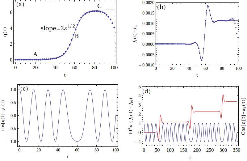
Figure 3: (a) The evolution of the variable $q(t)$ along the first homoclinic transition, as obtained by numerical integration in the complete model (2) (points), and with the model of Eq.(12) (solid curve). (b) The first observed numerical jump in $J_{1}(t)$ (points) against the prediction of the model of Eq.(13). (c) The curve $\cos(q(t)-\phi_{1}(t))$ in the time interval corresponding to the first jump. (d) Left axis: several jumps in the variable $J_{1}(t)$ compared with (right axis) the evolution of $\cos(q(t)-\phi_{1}(t))$. The jumps take place at precisely those points where the phase $q-\phi_{1}$ forms a local plateau, departing from a pure oscillation.

How can we understand this success of the ‘Melnikov approximation’? Of course the answer is hidden in the properties of the quadrature (13). As a coarse remark, by the equation for $\dot{J}_{1}(t)$ in (9)), the evolution of $J_{1}(t)$ is determined by the terms $\cos(q+\phi_{1})$, $\cos(q-\phi_{1})$ and $\cos\phi_{1}$. We saw that $\phi_{1}$ evolves nearly linearly $\phi_{1}(t)\approx\phi_{1}(0)+J_{10}t$, so the integral $\int_{0}^{t}\cos(\phi_{1}(t^{\prime}))dt^{\prime}\approx{1\over J_{10}}\sin(\phi_{1}(0)+J_{10}t)$ will only produce some rapid oscillation in the evolution of $J_{1}(t)$. The remaining terms, however, $\cos(q+\phi_{1})$, $\cos(q-\phi_{1})$ depend on the angle $q$, which evolves approximately by the pendulum trajectory of Eq. (12) (as shown in Fig. 3(a)). Now, the pendulum trajectory spends most of the time near the unstable origin, hence we have $\dot{q}\approx 0$ there. On the other hand the speed $\dot{q}$ in the middle of the homoclinic transition can be estimated as $\dot{q}(t)\approx 2\sqrt{\epsilon}$ (equal to $\dot{q}_{s}(t=T_{s}/2)$ in Eq. (12)). Thus, the curve $q(t)$ consists, essentially, of three parts, marked in Fig. 3(a) by A,B,and C respectively. In the domains A,C the curve is nearly horizontal, and $\cos(q\pm\phi_{1})\simeq\cos(\phi_{1})$, thus the integrals $\int\cos(q\pm\phi)$ yield essentially the same oscillatory behavior as for the integral $\cos\phi_{1}$ alone. In the domain $B$, instead, we have a slower evolution of the angle $q-\phi_{1}$: in our example we have $\dot{q}-\dot{\phi}_{1}\simeq 2\sqrt{\epsilon}-J_{10}=-0.07785...$ in B, compared to $\dot{q}-\dot{\phi}_{1}\simeq\sqrt{2\epsilon}=0.34...$, $J_{10}=0.4242...$ in A or C. As a consequence, The curve $\cos(q(t)-\phi_{1}(t))$ develops an approximate ‘plateau’ near the time $t=T_{s}/2\simeq 59.$ (Fig. 3(c)). Since the integrand of the Melnikov integral in (13) temporarily stabilizes to a constant value, the integral will give a locally linear evolution of $J_{1}(t)$, thus causing a quick jump, lasting roughly as the time duration of B. After exit from B, the $J_{1}(t)$ returns to an oscillatory evolution, which keeps up to the next homoclinic transition. More jumps then occur at each successive homoclinic transition, as shown in (Fig. 3(d)).

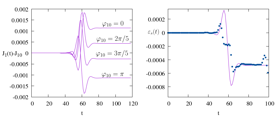
Figure 4: Left: the jumps in the variable $J_{1}$ obtained through formula (13) by changing the initial angle $\phi_{0}$ according to the values indicated in the figure. Right: The jump in the pendulum energy $\varepsilon_{s}=p^{2}/2+\epsilon(\cos q-1)$ as computed for the numerical orbit in the complete model (points) and with the ‘Melnikov model’ of Eq.(14).

Comparing the above picture with Fig.1(e), we do now interpret qualitatively the nature of the jumps, but we still need to understand why the jumps differ in size and/or sign. The sequences of times where jumps occur can be estimated by $t_{i+1}-t_{i}\approx T_{s}(\varepsilon_{s,i})$, with $T_{s}$ given by Eq. (11). These times are of similar order, but different one from the other even for a small change in $\varepsilon_{s}$ (compare the times $T_{s}$ when $\varepsilon_{s}=10^{-5}$ or $10^{-3}$). As a consequence, at the starting point of each homoclinic transition, the orbit is at a different value of the starting angle $\phi_{1,0}$. However, as shown in Fig. 4, according to the value of $\phi_{1,0}(t_{i})$ we can obtain jumps in $J_{1}$ of various sizes, positive or negative. Under the assumption that the sequence $\phi_{1,0}(t_{i})$ is random (‘random phase approximation’), this leads to a random walk model for the variations of $J_{1}(t)$. In reality, long correlations can survive in the sequence $\phi_{1,0}(t_{i})$, and the diffusion in $J_{1}(t)$ can partly loose its normal character (typically the dynamics becomes sub-diffusive, see [50]). Also, using the Melnikov approach, we may compute a continuous in time approximation for the evolution of the energy $\varepsilon_{s}(t)$

$$\varepsilon_{s}=\varepsilon-\frac{1}{2}(J_{1}^{(M)})(t))^{2}-J_{2}^{(M)}(t)-\epsilon\mu\left(\cos(q_{s}(t))-1\right)\left(\sin(\phi_{10}+J_{10}t)+\cos(\phi_{20}+t)\right)~{},$$ (14)

where $J_{2}^{(M)}(t)$ is the ‘Melnikov’ model for the evolution of the action $J_{2}$, analogous to the model (13) for the action $J_{1}$. The right panel in Fig. 4 shows the evolution of the pendulum energy $\varepsilon_{s}(t)$ for the first jump in the real orbit and as obtained by the model (14), showing again a good fit. Then using all the above approximations, we can arrive at a heuristic model for Chirikov’s ‘whisker map’. While deterministic, in practice this model leads to nearly random sequences $\varepsilon_{i}$, $\phi_{1,i}$, that is, to a stochastic process for the evolution of the orbit in the action space. Estimating the value of the diffusion coefficient relies on some semi-analytical approaches, as discussed in sections 3 and 4 below.

As a final comment, one can remark that the ‘plateaus’ of the curve $\cos(q-\phi_{1})$, responsible for the jumps Fig. 3(d), are due to the tuning of the values of $\dot{q}$ and $\dot{\phi}_{1}\simeq J_{10}$ at region B of Fig. 3. This tuning is rather exceptional, and was essentially imposed for illustration purposes by the choice of the initial condition $J_{10}$. Generic initial conditions instead (as, for example, choosing $J_{10}$ one order of magnitude larger) will destroy such tuning. Does this imply that there is no more drift in action space by jumps as the above? As will be discussed in section 4, we can make a number of steps of perturbation theory, seeking to eliminate altogether the now useless combinations $\cos(q-\phi_{1})$, $\cos(q+\phi)$ and prove perpetual stability for the actions $J_{1}$ and $J_{2}$. However, doing so generates new ‘dangerous’ harmonics along the normalization process (see, for example, [53]). As higher order harmonics $\cos(m_{q}q+m_{1}\phi_{1})$ are generated by the normalization, there will eventually appear some harmonics causing important jumps. Recalling that the jumps always take place in the domain B of Fig. 3(a), where the condition $\dot{q}\approx 2\sqrt{\epsilon}$ should hold, the tuning occurs for a harmonic satisfying $2m_{q}\sqrt{\epsilon}+m_{1}J_{10}\approx 0$. This implies a ratio $|m_{1}|/|m_{q}|={\cal O}(1/\sqrt{\epsilon})$. In Arnold’s model, such a harmonics will be generated for the first time at the normalization order $s_{0}=|m_{1}|+|m_{q}|={\cal O}(1/\sqrt{\epsilon})$. Then, it turns out that there is an optimal normalization order beyond which the critical harmonic can no longer be removed from the Hamiltonian. Usual normal form estimates (see section 4) lead to $s_{opt}={\cal O}(1/\mu^{b})$, for a positive exponent $b$. The size of the harmonic at optimal order will be ${\cal O}(\exp(1/\mu^{b}))$, i.e., i.e., exponentially small in $1/\mu$. This, yields, in general, an exponentially small drift velocity in action space.

An important remark regarding the precise estimates on the speed of Arnold diffusion is that the latter depend crucially on whether a system is a priori stable or a priori unstable (see also section 3 below). This distinction has been emphasized in a central paper on the subject by [11] (hereafter CG). That paper provides a rigorous proof of the occurrence of Arnold diffusion in a priori unstable systems and also along the simple resonances of a priori stable systems. It also discusses lower bounds on the times necessary for making ${\cal O}(1)$ excursions in action space. These bounds are estimated as exponentially small in $1/\mu^{2}$.

2.3 Geometric approach

The arguments exposed so far justify local variations in the values of the actions $J_{1}$ and $J_{2}$, but provide no theory for the long (${\cal O}(1)$) excursions of the trajectories in the action space. Demonstration that such excursions are possible requires, instead, the use of some geometric method. A standard method relies on the existence of orbits shadowing the heteroclinic intersections between the stable and unstable invariant manifolds emanating from the family of hyperbolic tori lying in the phase space of the system under study.

In Arnold’s example, these are the tori $\tau(J_{1},J_{2})$ defined in Eq. (3), which are quite distinct from the 3-dimensional KAM tori referred to subsection 2.1. In particular, along the tori $\tau(J_{1},J_{2})$ we always have the invariance $q(t)=p(t)=0$, corresponding to the hyperbolic fixed point of the pendulum. However, contrary to what we saw in the previous subsection, in the geometric method we seek to characterize the motions in the neighborhood of a hyperbolic torus $\tau(J_{1},J_{2})$ via the study of the invariant asymptotic manifolds emanating from the torus.

Consider first the case $\mu=0$. We define the stable and unstable manifolds, ${\cal W}^{U}_{(0,0)}$, ${\cal W}^{S}_{(0,0)}$ of the unstable fixed point of the pendulum as the set of all initial conditions $(q_{0},p_{0})$ whose time evolution leads to orbits $(q(t;q_{0},p_{0}),p(t;q_{0},p_{0})$ tending asymptotically to the unstable point $(0,0)$ as $t\rightarrow-\infty$ (for the unstable manifold) or $t\rightarrow\infty$ (for the stable manifold):

$${\cal W}^{U}_{(0,0)} = \left\{(q_{0},p_{0})\in\mathbb{T}\times\mathbb{R}:\lim_{t\rightarrow-\infty}(q(t;q_{0},p_{0}),p(t;q_{0},p_{0}))=(0,0)\right\}$$ (15)

$${\cal W}^{S}_{(0,0)} = \left\{(q_{0},p_{0})\in\mathbb{T}\times\mathbb{R}:\lim_{t\rightarrow\infty}(q(t;q_{0},p_{0}),p(t;q_{0},p_{0}))=(0,0)\right\}~{}~{}.$$

For $\mu=0$ the sets ${\cal W}^{U}_{(0,0)}$, ${\cal W}^{S}_{(0,0)}$ coincide, as they both correspond to the pendulum separatrix. Consider, now, the following set of initial conditions of the full problem:

$${\cal Q}_{0}:J_{1}(0)=J_{10},~{}~{}J_{2}(0)=J_{20},~{}~{}\phi_{1}(0)=\phi_{10},~{}~{}\phi_{2}(0)=\phi_{20}$$

$$(q(0)=q_{0},p(0)=p_{0})\in{\cal W}^{S}_{(0,0)}~{}~{}.$$

Since $\mu=0$ the variables $(q,p)$ evolve independently from the variables $(\phi,J)$. Since $(q_{0},p_{0})\in{\cal W}^{S}_{(0,0)}$, $(q(t),p(t))$ will tend to $(0,0)$ as $t\rightarrow\infty$, while $(\phi,J)$ will have an identical evolution as in the torus $\tau(J_{1},J_{2})$. Hence, the trajectory tends to the torus $\tau(J_{10},J_{20})$ as $t\rightarrow\infty$. We then define the stable and unstable manifolds of a torus $\tau(J_{1},J_{2})$ as:

$${\cal W}^{U}_{\tau(J_{1},J_{2})} = \left\{{\cal Q}_{0}\in\mathbb{T}^{3}\times\mathbb{R}^{3}:\lim_{t\rightarrow-\infty}\mbox{dist}\left({\cal Q}(t;{\cal Q}_{0}),\tau(J_{1},J_{2})\right)=0\right\}$$ (17)

$${\cal W}^{S}_{\tau(J_{1},J_{2})} = \left\{{\cal Q}_{0}\in\mathbb{T}^{3}\times\mathbb{R}^{3}:\lim_{t\rightarrow\infty}\mbox{dist}\left({\cal Q}(t;{\cal Q}_{0}),\tau(J_{1},J_{2})\right)=0\right\}$$

where ${\cal Q}(t;{\cal Q}_{0})\in\mathbb{T}\times\mathbb{R}^{3}$ denotes the trajectory (in all six variables) corresponding to the initial condition ${\cal Q}_{0}$.

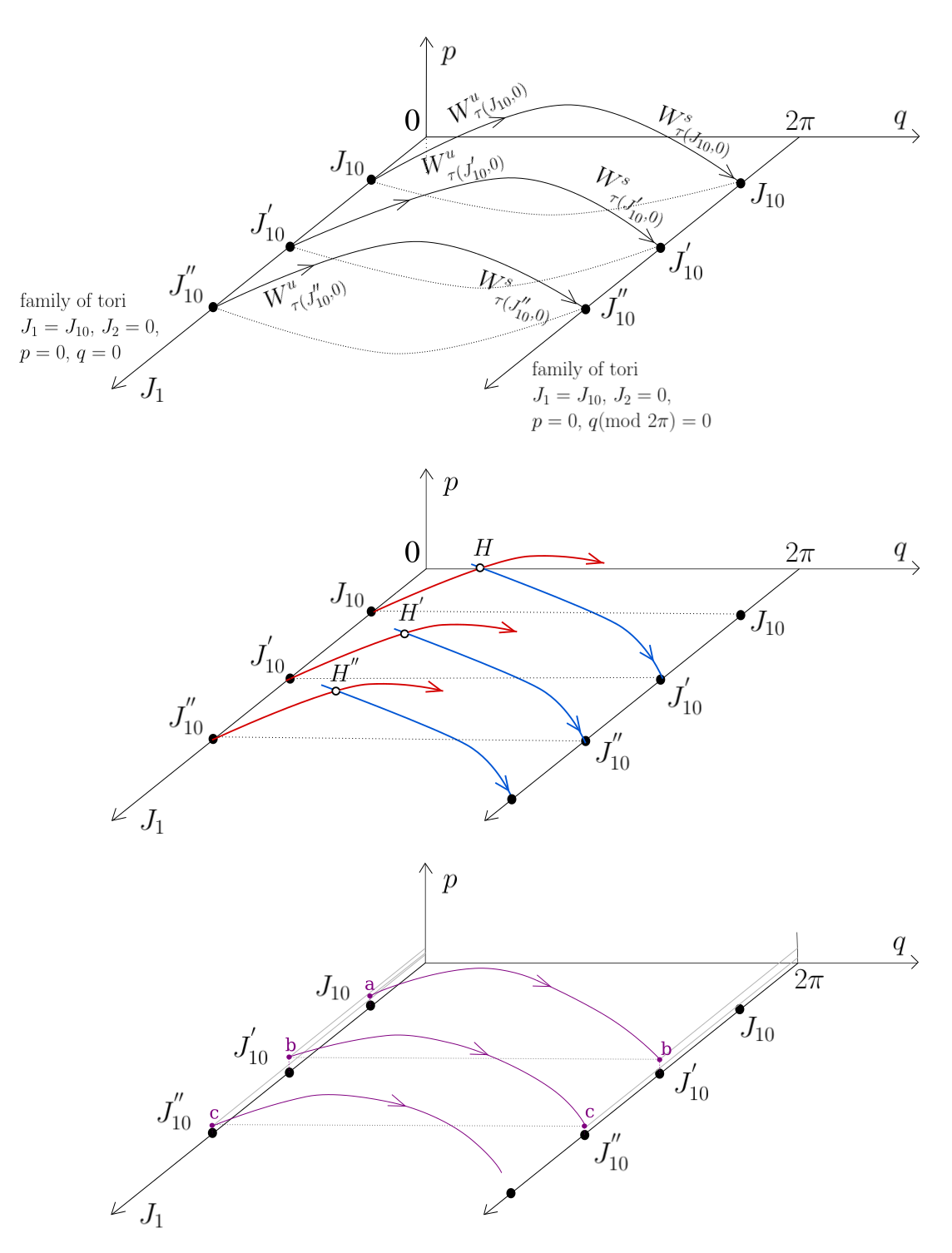
Figure 5: Schematic representation of Arnold’s mechanism: Top: When $\mu=0$, the ‘whiskers’ (stable and unstable manifolds) of three nearby hyperbolic 2D tori labeled by the actions $J_{10}$, $J_{10}^{\prime}$ and $J_{10}^{\prime\prime}$ are joined smoothly as pendulum separatrices. Middle: For $\mu\neq 0$, the unstable manifolds (red) of one torus intersect heteroclinically with the stable manifolds (blue) of a nearby torus. This establishes a ‘chain’ of heteroclinic connections. Bottom: There is a true orbit (purple) ‘shadowing’ the above chain, that is, undergoing Arnold diffusion.

We saw that the invariant tori $\tau(J_{1},J_{2})$ (with $q=p=0$) continue to exist when $\mu\neq 0$. Is it, however, possible to find initial conditions ${\cal Q}_{0}$ satisfying the definition of the stable and unstable manifolds ${\cal W}^{S}_{\tau(J_{1},J_{2})}$, ${\cal W}^{U}_{\tau(J_{1},J_{2})}$ when $\mu\neq 0$? The answer to this question is affirmative. In fact, a local normal form around the torus $\tau(J_{1},J_{2})$ allows to give in parametric form initial conditions in the neighborhood of the torus which satisfy the manifold definition. Then, propagating these local initial conditions backwards of forwards in time, respectively, we can unfold the whole set of initial conditions belonging to the manifolds ${\cal W}^{S}_{\tau(J_{1},J_{2})}$, ${\cal W}^{U}_{\tau(J_{1},J_{2})}$ in the perturbed case as well. However, as argued by Arnold([2]; see also [11]), the manifolds emanating from different tori in the perturbed system $\mu\neq 0$ have a property not holding when $\mu=0$, namely, manifolds of tori corresponding to the same energy but being sufficiently close to each other can intersect heteroclinically, i.e. the unstable manifold of one torus can interest with the stable manifold of a nearby torus and vice versa. Figure 5 shows schematically what happens with the manifolds of the tori $\tau(J_{1},J_{2})$ in Arnold’s model (2): Consider a fixed value of the energy $E$. On one such torus we have $q=p=0$, thus $E=J_{1}^{2}/2+J_{2}$. For every initial condition with $J_{1}=J_{1,0}$ we can specify $J_{2}=E-J_{1}^{2}/2$, and thus define the torus $\tau(J_{1}=J_{10},J_{2}=E-J_{1}^{2}/2$. In reality, since $J_{2}$ is a dummy action variable measuring the change of energy in the non-autonomous system (1), which is equivalent to the system (2), only the action $J_{10}$ truly labels different tori. Hence, for different values of $J_{10}$ we obtain a family of tori, denoted by $\tau(J_{10},0)$, for different values of the constant $J_{10}$. The top panel of Fig. 5 shows three such tori, $\tau(J_{10},0)$, $\tau(J_{10}^{\prime},0)$, $\tau(J_{10}^{\prime\prime},0)$, corresponding to three points on the axis $J_{1}$ of the figure. In reality, the tori are not points, but they are parameterized by the angles $\phi_{1},\phi_{2}$ given by all possible trajectories $\phi_{1}(t)=\phi_{10}+J_{10}t$, $\phi_{2}=t$. These angular variables are not included in the schematic figure 5.

Now, from every torus $\tau(J_{10},0)$ emanate the stable and unstable manifolds ${\cal W}^{S}_{\tau(J_{10},0)}$, ${\cal W}^{U}_{\tau(J_{10},0)}$. In the case $\mu=0$, we saw that these manifolds join each other smoothly, as they actually coincide with the pendulum separatrix. Hence, as shown in the top panel of Fig. 5, the manifolds of different tori cannot intersect, i.e., ${\cal W}^{U}_{\tau(J_{10},0)}$ cannot intersect with ${\cal W}^{S}_{\tau(J_{10}^{\prime},0)}$, ${\cal W}^{U}_{\tau(J_{10}^{\prime},0)}$ cannot intersect with ${\cal W}^{S}_{\tau(J_{10}^{\prime\prime},0)}$, etc., no matter how close the tori $\tau(J_{10},0)$, $\tau(J_{10}^{\prime},0)$, $\tau(J_{10}^{\prime\prime},0)$ are one to the other. However, this changes when $\mu\neq 0$, and it can be demonstrated that if $\tau(J_{10},0)$ is taken sufficiently close to $\tau(J_{10}^{\prime},0)$, the manifolds ${\cal W}^{U}_{\tau(J_{10},0)}$ and ${\cal W}^{S}_{\tau(J_{10}^{\prime},0)}$ can intersect. The middle panel of Fig. 5 shows such an intersection, at the point H, called a heteroclinic point. The sequence of the heteroclinic points H,H’,H” of the middle panel of Fig. 5 will be called a ‘heteroclinic chain’. The sequence of tori whose manifolds yield the points H,H’,H” are known with various names, namely, the Arnold chain of ‘whiskered tori’ (the manifolds are the ‘whiskers’), or the ‘diffusion path’ (see [11]).

Consider, finally, the past and future trajectories with initial conditions corresponding to the points H,H’,H”, etc. The trajectory from H belongs to both the invariant manifolds ${\cal W}^{U}_{\tau(J_{10},0)}$ and ${\cal W}^{S}_{\tau(J_{10}^{\prime},0)}$. Thus, in the limit $t\rightarrow\-\infty$ the trajectory tends to the torus $\tau(J_{10},0$, while, in the limit $t\rightarrow\infty$ the trajectory tends to the torus $\tau(J_{10}^{\prime},0$. This implies that this particular trajectory undergoes no large excursion in the action space, since its past and future is confined between two nearby asymptotic limits. Similarly, the past and future from the heteroclinic point H’ connect the tori $\tau(J_{10}^{\prime},0)$ with $\tau(J_{10}^{\prime\prime},0)$, those from the heteroclinic point H” connect the tori $\tau(J_{10}^{\prime\prime},0)$ with $\tau(J_{10}^{\prime\prime\prime},0)$, etc., but the corresponding trajectories make only bounded excursions in the action space. However, employing a so-called shadowing lemma, it is possible to demonstrate that there is one continuous in time trajectory of the system which remains piece-wise close (i.e. ‘shadows’) any one of the distinct heteroclinic trajectories from the points $H$,$H^{\prime}$,$H^{\prime\prime}$,… Such a trajectory is shown schematically in the last panel of Fig. 5. It is precisely this trajectory which materializes the ‘Arnold’s mechanism’ referred to in the introduction. Extending the heteroclinic chain $H,H^{\prime},H^{\prime\prime},...,H^{(n)},...$ to include more heteroclinic points, one can find a trajectory connecting the neighborhoods of the initial torus $\tau(J_{10},0)$ and another torus $\tau(J_{10}^{(n)},0)$ located at arbitrarily large distance from $\tau(J_{10},0)$ (possibly limited only by the requirement of the two tori being isoenergetic).

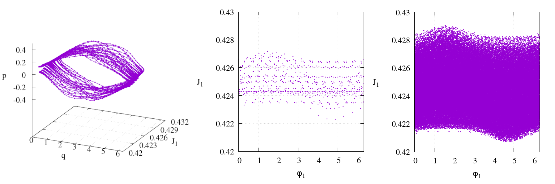
Figure 6: Left: Real (non-schematic) orbit shadowing the intersecting manifolds of nearby tori in Arnold’s model, obtained by plotting in the $(p,q)\times J_{1}$ space the same orbit as in Fig. 1, for the integration time $t=700$. Center and Right: the projection of the orbit on the $(\phi_{1},J_{1})$ plane at two different integration times, $t=700$ and $t=150000$.

Does the ‘Arnold mechanism’ interpret the long-term evolution of the numerical trajectory used in our example in the previous subsection? Figure 6 suggests this to be so, provided that the trajectory is integrated for times much longer than those referred to in the previous subsection. The left panel shows how the trajectory produced by integration of the complete model (2), and with the same initial conditions as in Fig. 1 shadows the whiskers of nearby tori $\tau(J_{1},J_{2})$. The middle and right panels show the projection of the trajectory in the plane $(\phi_{1},J_{1}$. Clearly, the trajectory remains piece-wise close to various rotational tori (corresponding to different values of $J_{1}$), however, as the integration time extends from $t=700$ to $t=1.5\times 10^{5}$ the excursion in $J_{1}$ extends from a total size $\sim 10^{-2}$ to nearly $\sim 10^{-1}$. Note that as the trajectory reaches domains further and further away from this particularly selected initial condition, the drift in action space actually gets slower (see last paragraph of subsection 2.2).

As a final remark, the above geometric picture of intersecting manifolds can be extended, from the chain of nearby tori, to include the whole invariant set ${\cal T}$ of the tori $\tau(J_{1},J_{2})$. This is a four-dimensional subset of $\mathbb{R}^{2}\times\mathbb{T}^{2}$, which is normally hyperbolic (see [21] for definitions). Normal hyperbolicity implies the existence of a stable and unstable manifold for the whole invariant set $\cal{T}$. Since, in Arnold’s example, $\cal{T}$ is just foliated by the tori $\tau{J_{1},J_{2}}$, the manifolds ${\cal W}^{U}_{\cal T}$, ${\cal W}^{S}_{\cal T}$ are just the union of the unstable and stable manifolds of all the tori. Homoclinic orbits can then be described by a ‘scattering map’ indicating how a point on ${\cal T}$ is mapped asymptotically in time to another point on ${\cal T}$ via a doubly-asymptotic orbit.

3 A priori stable systems - Nekhoroshev theory

Consider the following Hamiltonian in action-angle variables, which, according to Poincaré [56], represents the “fundamental problem of dynamics”:

$$H(\phi,I)=H_{0}(I)+\epsilon H_{1}(\phi,I)$$ (18)

with $\phi\in\mathbb{T}^{n}$, $I\in\mathbb{R}^{n}$.

For $\epsilon=0$ the system is integrable $H=H_{0}(I)$ and the phase space is foliated by invariant tori labeled by the constant actions $I$. On each torus the angles evolve linearly with the frequencies $\omega(I)=\nabla_{I}H_{0}(I)$. Periodic orbits, or, in general, tori of dimension $n^{\prime}<n$ correspond to values of the actions $I$ for which the frequencies $\omega(I)$ satisfy $n-n^{\prime}$ commensurability conditions. However, all these low-dimensional objects are neutral in stability, and there are no separatrices or any other type of asymptotic manifolds (‘whiskers’) associated to them. In other words, there is no in-built hyperbolicity in the Hamiltonian $H_{0}(I)$. Hence, invariant objects of (partially) hyperbolic character can only be born by setting $\epsilon\neq 0$. Such systems were thus called (by CG) ‘a priori stable’.

The lack of invariant phase space objects with inherent hyperbolicity generates several challenging new questions regarding Arnold diffusion. We now summarize some of these questions as well as known results related to Arnold diffusion in a priori stable systems.

3.1 Nekhoroshev theory and exponential stability

Whatever the mechanism possible to cause Arnold diffusion in an a priori stable system, the speed of the drift in action space in such a system is bounded before all by the Nekhoroshev theorem ([55], [3], [4],[48], [57]):

Nekhoroshev theorem: Assume a Hamiltonian of the form (18) with $\epsilon>0$, with $H$ analytic in a complex extension ${\cal D}$ of the set $D\times\mathbb{T}^{n}$, where $D\subset\mathbb{R}^{n}$ is open, and $H_{1}$ bounded. Assume that $H_{0}$ satisfies suitable steepness conditions. Then, there are positive constants $a,b,\epsilon_{0}$ such that, for $\epsilon<\epsilon_{0}$ and for all initial conditions in ${\cal D}$, under the flow of the Hamiltonian $H$ we have:

$$|J(t)-J(0)|<\epsilon^{a}~{}~{}~{}\mbox{for all times~{}$t<T_{N}$ with~{}}T_{N}={\cal O}\left({\epsilon_{0}\over\epsilon}\exp((\epsilon_{0}/\epsilon)^{b})\right)$$ (19)

We refer to $T_{N}$ as the ‘Nekhoroshev time’. A detailed discussion of the meaning and importance of ‘steepness’ in the above theorem is made in [39][60][12]. We briefly refer to steepness in subsection 3.2 below.

Demonstration of the Nekhoroshev Theorem (see [34] for a tutorial) requires combining an analytical with a geometric part. The analytical part deals with the local construction of a ‘Nekhoroshev normal form’, whose remainder at the optimal normalization order turns to be exponentially small. On the other hand, the geometric part deals with the construction of a set of subdomains $D_{1},D_{2},\ldots\subset{\cal D}$ defined so that: i) a different local normal form with exponentially small remainder can be constructed in each domain, and ii) the union of all domains provides a covering of ${\cal D}$. The structure of resonant manifolds (see below), depending on the form of the integrable part $H_{0}(I)$ of the Hamiltonian, as well as the size of the analyticity domain around each manifold, determined by the form of $H_{1}(\phi,I)$, are crucial factors in the appropriate definition of the domains $D_{i}$. In particular, the domains $D_{i}$ must have size depending algebraically on $\epsilon$, i.e. $\mbox{diam}(D_{i})={\cal O}(\epsilon^{a_{i}})$, $a_{i}>0$. One then demonstrates that this dependence allows to obtain a covering of ${\cal D}$ by combining many such domains when $\epsilon$ is arbitrarily small (see [54] for a heuristic argument). Now, the size of the optimal remainder of each local normal form scales as $||R||=O\left(-\exp((\epsilon_{0,i}/\epsilon)^{b_{i}})\right)$, for some positive constant $\epsilon_{0,i}$ and positive exponent $b_{i}$. Choosing the worst possible combination $a_{i},b_{i}$ and $\epsilon_{i,0}$ from those holding in each domain allows to arrive at the global bound (19). In practice, locally we can obtain better bounds using the local parameters $a_{i},b_{i},\epsilon_{0,i}$. It turns out that the exponents $a,b$ depend on i) the number of degrees of freedom $n$, ii) the so-called steepness indices holding within the domain (see [39] for definitions) and, finally, iii) the multiplicity of the local resonance considered (see below).

It is noteworthy that, while in the proof of the theorem the analytical part plays a minimal role, the actual construction of the Nekhoroshev normal form in any explicit application implies reaching a very high order of normalization, involving typically millions of operations that can only be carried out with the aid of a computer-algebraic program. Starting from the sixties ([15],[16], [36], [35]), such programs dealt first with the simpler case of systems with elliptic equilibria, such as the celebrated Hénon-Heiles system [41]. In such systems, exponential estimates can be obtained without the need of a geometric construction as the one of the Nekhoroshev theorem. Well known applications in Celestial Mechanics have been given, referring, for example, to the long term stability of the Trojan asteroids of Jupiter [9][33][23][47], the spin-orbit problem [59], and the $J_{2}$ problem of satellite motions [61][18]. On the other hand, computing the optimal Nekhoroshev normal form in a generic Hamiltonian of the form (18) has been possible so far only in simple models with $n=3$ degrees of freedom [24][26][14] [40]. Such computations allow for a direct comparison between ‘semi-analytical’ (i.e. by the remainder of the Nekhoroshev normal form) and numerical results on the speed of Arnold diffusion, as well as on the adiabatic evolution of the action variables in a priori stable systems. Most notable among the numerical experiments are those carried over the years by the group of C. Froeschlé, M. Guzzo and E. Lega ([44][37] [30][39]), which have given clear evidence of the occurrence of Arnold diffusion in a priori stable systems. A comparison of the exponents $a,b$ found by the Nekhoroshev normal form construction and by the numerical experiments has shown a very good agreement. This has extended also to estimates on the coefficient of Arnold diffusion as well as to the modeling of the jumps carried by the adiabatic action variables along the heteroclinic transitions taking place in single resonance domains. In the sequel we give a summary of the above results with the help (as in the previous section) of a simple example of a priori stable system with $n=3$ degrees of freedom.

3.2 A simple example

Consider the 3DOF Hamiltonian in action-angle variables:

$$H=H_{0}+\epsilon H_{1}=\frac{I_{1}^{2}}{2}-\frac{I_{2}^{2}}{2}+\frac{I_{2}^{3}}{3\pi}+2\pi I_{3}+{\epsilon\over 4+\cos\phi_{1}+\cos\phi_{2}+\cos\phi_{3}}~{}~{}.$$ (20)

The Hamiltonian (20) has been used in [40] in the study of the evolution of the adiabatic action variables. An analogous 4D symplectic mapping was used in [39] for the study of the effects of steepness on the stability of the orbits.

The flow corresponding to the integrable part of (20)

$$H_{0}=\frac{I_{1}^{2}}{2}-\frac{I_{2}^{2}}{2}+\frac{I_{2}^{3}}{3\pi}+2\pi I_{3}~{}~{}.$$ (21)

is given by $\dot{I_{i}}=0$, $i=1,2,3$ and $\dot{\phi}_{1}=\omega_{0,1}=I_{1}$, $\dot{\phi}_{2}=\omega_{0,2}=-I_{2}+\frac{1}{\pi}I_{2}^{2}$, $\dot{\phi}_{3}=\omega_{0,3}=2\pi$. Thus, all trajectories lie on invariant tori labeled by the actions $I_{i}$ or the corresponding frequencies $\omega_{0,i}$.

Let $k\equiv(k_{1},k_{2},k_{3})\in\mathbb{Z}^{3}$. We call resonant manifold ${\cal RM}(k_{1},k_{2},k_{3})$ associated to the Hamiltonian $H_{0}$ the two-dimensional manifold

$${\cal RM}(k_{1},k_{2},k_{3}) := \bigg{\{}(I_{1},I_{2},I_{3})\in\mathbb{R}^{3}:$$

$$k\cdot\omega_{0}(I)=k_{1}I_{1}+k_{2}(-I_{2}+\frac{1}{\pi}I_{2}^{2})+k_{3}\,2\pi=0\bigg{\}}~{}~{}.$$

We call energy manifold ${\cal E}(E)$ the two-dimensional manifold

$${\cal E}(E):=\left\{(I_{1},I_{2},I_{3})\in\mathbb{R}^{3}:~{}~{}H_{0}(I)={1\over 2}(I_{1}^{2}-I_{2}^{2})+\frac{I_{2}^{3}}{3\pi}+2\pi I_{3}=E\right\}~{}~{}.$$ (23)

Figure 7(a) shows a part of the energy manifold ${\cal E}(E)$ for $E=1$ as well as parts of the two resonant manifolds ${\cal RM}(1,1,0)$ and ${\cal RM}(4,-1,-1)$. The set of all curves formed by the intersection of all resonant manifolds ${\cal RM}(k)$, $k\in\mathbb{Z}^{3}$, $|k|\neq 0$ with the energy manifold ${\cal E}(E)$ is called the Arnold web (or ‘web of resonances’). In our example, the definition of the resonant manifolds via Eq. (3.2) does not depend on $I_{3}$. Thus all resonant manifolds intersect normally the plane $(I_{1},I_{2})$ at curves given by Eq. (3.2). Figure 7(b) shows some of these resonant curves marked with the corresponding integers $(k_{1},k_{2},k_{3})$.

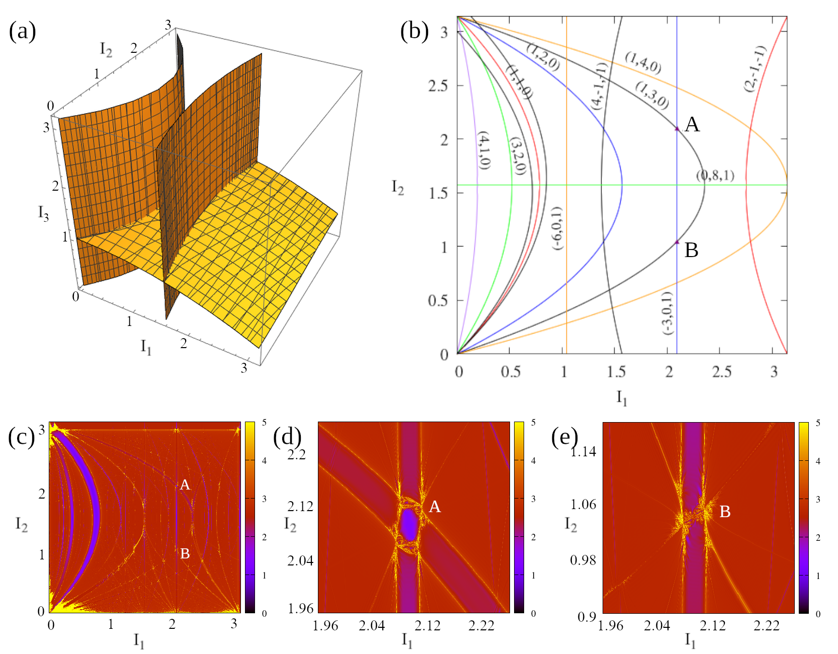
Figure 7: (a) Part of the energy manifold ${\cal E}(E)$ in the model (21) for $E=1$ (yellow), intersected by parts of the resonant manifolds ${\cal RM}(1,1,0)$ and ${\cal RM}(4,-1,-1)$ (orange). (b) Projection of the Arnold web of resonances on the $(I_{1},I_{2})$ plane. For the resonance (1,1,0) the corresponding separatrix borders are also displayed as computed theoretically for $\epsilon=0.05$ (see text). (c) FLI stability map for the Hamiltonian (20) with $\epsilon=0.05$. The web of resonances is visualized through the detection of weakly chaotic orbits at the borders of each resonance. (d) and (e) Details of figure (c) around the resonance junctions A and B, respectively, where the resonant manifolds ${\cal RM}(1,3,0)$ and ${\cal RM}(3,0,-1)$ intersect.

The set of the resonant curves defined by all possible $(k_{1},k_{2},k_{3})\in\mathbb{Z}^{3}$, $|k|\neq 0$ is dense in the square $S(I_{1},I_{2})$ depicted in Fig. 7(b): for any open, small whatsoever, neighborhood $S_{i}\subset S(I_{1},I_{2})$ there exist integers$(k_{1},k_{2},k_{3})$ such that the corresponding resonant curve crosses $S_{i}$. However, not all these resonances are equally important for dynamics. This is evidenced by computing a stability map in the same square $S(I_{1},I_{2})$ via the use of a chaotic indicator. Figure 7(c) shows the stability map computed by the Fast Lyapunov Indicator (FLI, [28] and the chapter by Guzzo and Lega in this book) in a grid of initial conditions for $(I_{1},I_{2})$, setting initially $I_{3}=\phi_{1}=\phi_{2}=\phi_{3}=0$, and for an integration time $t=1000$. We immediately note that the FLI map in Fig. 7(c) is able to depict the structure of the Arnold web in great detail. This fact, first found in [29] has played a crucial role in the numerical study of Arnold diffusion in a priori stable systems.

In Fig. 7(c) we see that the most prominent structures are related to low order resonances ($|k|=|k_{1}|+|k_{2}|+|k_{3}|$ small). Also, we notice that, for some resonances (e.g. (1,1,0)), the FLI map shows a double set of curves going nearly parallel one to the other along the resonance, with a blue zone between the curves. Other resonances, instead, are identified by a single line (yellow). This distinction depends on the sign of the Fourier coefficient of the corresponding resonant harmonics in the function $H_{1}$ of Eq. (20). We have:

$${1\over 4+\cos\phi_{1}+\cos\phi_{2}+\cos\phi_{3}}=\sum_{k_{1},k_{2},k_{3}=-\infty}^{\infty}h_{k_{1},k_{2},k_{3}}\cos(k_{1}\phi_{1}+k_{2}\cos\phi_{2}+k_{3}\phi_{3})$$

where $h_{k_{1},k_{2},k_{3}}$ can be easily computed expanding the denominator in Taylor series and using the trigonometric reduction formulas. Consider a toy Hamiltonian in which only one harmonic is isolated:

$$H_{res}=\frac{I_{1}^{2}}{2}-\frac{I_{2}^{2}}{2}+\frac{I_{2}^{3}}{3\pi}+2\pi I_{3}+\epsilon h_{k_{1},k_{2},k_{3}}\cos(k_{1}\phi_{1}+k_{2}\cos\phi_{2}+k_{3}\phi_{3})~{}~{}.$$ (24)

Such a model will be obtained by just performing one step of perturbation theory eliminating from the Hamiltonian (20) all other harmonics except for the resonant one (see section 4). Now, the Hamiltonian (24) is integrable. To show this, assume (without loss of generality) $k_{1}\neq 0$. Consider two linearly independent integer vectors $m,n\in\mathbb{Z}^{3}$ such that $m\cdot k=n\cdot k=0$ (for example $m=(k_{2},-k_{1},0)$, $n=(k_{3},0,-k_{1})$). Consider the canonical transformation $(\phi_{1},\phi_{2},\phi_{3},I_{1},I_{2},I_{3})$ $\rightarrow$ $(\phi_{R},\phi_{F1},\phi_{F2},I_{R},I_{F1},I_{F2})$ defined by

$$\phi_{R}=k\cdot\phi,\phi_{F1}=m\cdot\phi,\phi_{F2}=n\cdot\phi~{}~{},$$

as well as the inverse of the equations

$$I_{1} = k_{1}I_{R}+m_{1}I_{F1}+n_{1}I_{F2},$$

$$I_{2} = k_{2}I_{R}+m_{2}I_{F1}+n_{2}I_{F2},$$ (25)

$$I_{3} = k_{3}I_{R}+m_{3}I_{F1}+n_{3}I_{F2}~{}~{}.$$

Substituting these expressions into (24) we arrive at:

$$H_{res}=H_{0}(I_{R},I_{F1},I_{F2})+\epsilon h_{k_{1},k_{2},k_{3}}\cos(\phi_{R})~{}~{}.$$ (26)

Since the angles $\phi_{F1},\phi_{F2}$ are ignorable, the above model has two integrals of motion $I_{F1},I_{F2}$ besides the energy. We are interested in studying the behavior of the model $H_{res}$ in a neighborhood around values $(I_{1*},I_{2*},I_{3*})$ which satisfy the resonance exactly. Setting $I_{i}=I_{i*}+J_{i}$, $i=1,2,3$ and substituting into (24) we arrive at:

$$H_{0}(J) = H_{0}(I_{*})+\nabla_{I}H_{0}(I_{*})\cdot J+{1\over 2}\sum_{i=1}^{3}\sum_{j=1}^{3}{\partial^{2}H_{0}(I_{*})\over\partial I_{i}\partial I_{j}}J_{i}J_{j}$$

$$+ {1\over 6}\sum_{i=1}^{3}\sum_{j=1}^{3}\sum_{l=1}^{3}{\partial^{3}H_{0}(I_{*})\over\partial I_{i}\partial I_{j}\partial I_{l}}J_{i}J_{j}J_{l}+\ldots~{}~{}.$$

The constant term $H_{0}(I_{*})$ can be omitted. The term $\nabla_{I}H_{0}(I_{*})\cdot J$ has the form

$$\nabla_{I}H_{0}(I_{*})\cdot J=(k\cdot\omega_{*})J_{R}+(m\cdot\omega_{*})J_{F1}+(n\cdot\omega_{*})J_{F2}=(m\cdot\omega_{*})J_{F1}+(n\cdot\omega_{*})J_{F2}~{}~{}.$$

where $\omega_{*}$ denotes the vector of the resonant frequencies $\omega_{i*}=\omega_{i}(I_{*})$, and the variables $J_{R},J_{F1},J_{F2}$ are defined as $J_{R}=I_{R}-I_{R*}$, $J_{F1}=I_{F1}-I_{F1*}$, $J_{F2}=I_{F2}-I_{F2*}$ with

$$\left(\begin{array}[]{c}I_{R*}\\ I_{F1*}\\ I_{F2*}\end{array}\right)=\left(\begin{array}[]{ccc}k_{1}&m_{1}&n_{1}\\ k_{2}&m_{2}&n_{2}\\ k_{3}&m_{3}&n_{3}\end{array}\right)\left(\begin{array}[]{c}I_{1*}\\ I_{2*}\\ I_{3*}\end{array}\right)$$

The frequencies $\omega_{*}$ satisfy $k\cdot\omega_{*}=0$, hence the transformed Hamiltonian contains linear terms only for the ‘fast’ action variables $J_{F1},J_{F2}$. Instead, the resonant action $J_{R}$ appears in the Hamiltonian only in quadratic terms (or of higher degree) in the actions. Setting the integrals as $J_{F1}=0$, $J_{F2}=0$ implies the relations $I_{F1}=I_{F1*}$, $I_{F2}=I_{F2*}$, that is:

$$I_{1} = k_{1}I_{R}+m_{1}I_{F1*}+n_{1}I_{F2*}$$

$$I_{2} = k_{2}I_{R}+m_{2}I_{F1*}+n_{2}I_{F2*}$$ (28)

$$I_{3} = k_{3}I_{R}+m_{3}I_{F1*}+n_{3}I_{F2*}$$

Thus, the motion in all three action variables under the flow of the model Hamiltonian (24) is determined by the only evolving action, namely $I_{R}$, and it is confined along a line ${\cal L}(I_{*})$ in the space $(I_{1},I_{2},I_{3})$ defined parametrically by Eq. (3.2). The projection of the line ${\cal L}(I_{*})$ on the plane $(I_{1},I_{2})$ is given by

$$I_{2}={1\over k_{1}}\left(-k_{2}I_{I}+(k_{2}m_{1}-k_{1}m_{2})I_{F1*}+(k_{2}n_{1}-k_{1}n_{2})I_{F2*}\right)$$ (29)

Also, the only non-ignorable angle in the model Hamiltonian of the resonance is $\phi_{R}\in\mathbb{T}$. The set ${\cal P}_{F}(I_{*})={\cal L}(I_{*})\times\mathbb{T}$ is called plane of fast drift. On this plane the motion is described by a pendulum-like Hamiltonian in the local variables $(\phi_{R},J_{R})$. The equations (3.2) imply $J_{R}=(k\cdot J)/(k\cdot k)$. Then, the quadratic term in the actions in (3.2) takes the form:

$${1\over 2}\sum_{i=1}^{3}\sum_{j=1}^{3}{\partial^{2}H_{0}(I_{*})\over\partial I_{i}\partial I_{j}}J_{i}J_{j}={1\over 2}\beta(I_{*})J_{R}^{2}~{}~{}\mbox{with}~{}~{}\beta(I_{*})={1\over k^{2}}(M(I_{*})k)\cdot k$$ (30)

where $M(I_{*})$ is the $3\times 3$ Hessian of the Hamiltonian $H_{0}$ calculated at the point $I_{*}$

$$M_{ij}(I_{*})=\left({\partial^{2}H_{0}\over\partial I_{i}\partial I_{j}}\right)_{I=I_{*}}$$

Similarly, the cubic term in the actions takes the form $(1/3)\gamma(I_{*})J_{R}^{3}$ with

$$\gamma(I_{*})={1\over 2|k|^{3/2}}\sum_{i=1}^{3}\sum_{j=1}^{3}\sum_{l=1}^{3}\left({\partial^{3}H_{0}(I_{*})\over\partial I_{i}\partial I_{j}\partial I_{l}}\right)_{I=I_{*}}k_{i}k_{j}k_{l}$$ (31)

Hence, apart from constants we have

$$H_{res}={1\over 2}\beta(I_{*})J_{R}^{2}+{1\over 3}\gamma(I_{*})J_{R}^{3}+\epsilon h_{k}\cos(\phi_{R})$$ (32)

where, in the model (21) we get:

$$\beta(I_{*})=k_{1}^{2}+k_{2}^{2}\left({2I_{2*}\over\pi}-1\right),~{}~{}~{}\gamma(I_{*})={k_{2}^{3}\over\pi}$$ (33)

Except for the case $k_{1}=k_{2}$ and $I_{2*}\rightarrow 0$, the coefficient $\beta(I_{*})$ is in general a ${\cal O}(1)$ quantity. Then, taking $J_{R}$ in a domain of size ${\cal O}(\epsilon^{1/2})$, the term ${1\over 2}\beta(I_{*})J_{R}^{2}$ is more important than the term ${1\over 3}\gamma(I_{*})J_{R}^{3}$ in $H_{res}$. This means that $H_{res}$ (ignoring cubic terms) becomes a pendulum Hamiltonian with separatrices extending in a domain $J_{R,min}\leq J_{R}\leq J_{R,max}$ estimated by:

$$J_{R,min}\simeq-2\left({\epsilon\over|\beta(I_{*})|}\right)^{1/2},~{}~{}~{}J_{R,max}\simeq 2\left({\epsilon\over|\beta(I_{*})|}\right)^{1/2}~{}~{}.$$ (34)

In reality, the motion very close to the separatrix will be weakly chaotic, due to the fact that, as discussed below, the remaining resonances can be eliminated only up to an exponentially small remainder, and hence there is some degree of chaos due to the interaction of these resonances with the principal one $(k_{1},k_{2},k_{3})$. The motion along the separatrix-like thin chaotic layer of the resonance can be projected also on the plane $(I_{1},I_{2})$. The projection is constrained in a segment along the line ${\cal L}(I_{*})$, which represents the intersection of the plane of fast drift with the plane $(I_{1},I_{2})$. In particular, the motion along the separatrix layer projects to a linear segment given by Eq. (3.2), setting $I_{R}=I_{R*}+J_{R}$, and varying $J_{R}$ in the limits $J_{R,min}\leq J_{R}\leq J_{R,max}$.

We are now able to understand the structure of the FLI map shown in Fig. 7(c). Let $I_{*}$ be one point along the resonance $(k_{1},k_{2},k_{3})$. Since in the computation of the FLI we have set the initial conditions $\phi_{i}=0$, $i=1,2,3$, the FLI map intersects the plane of fast drift crossing the point $I_{*}$ at the value $\phi_{R}=0$. Whenever the coefficients $\beta(I_{*})$ and $h_{k_{1},k_{2},k_{3}}$ have the same sign, the point $\phi_{R}$ represents the unstable equilibrium point of the Hamiltonian $H_{res}$. One has $J_{R}=0$ there, thus, by Eqs. (3.2) we get a unique point on the FLI map, given by $I_{1}=I_{1*}$, $I_{2}=I_{2*}$. On the contrary, when $\beta(I_{*})$ and $h_{k_{1},k_{2},k_{3}}$ have opposite signs, the point $\phi_{R}$ corresponds to the stable equilibrium point of the Hamiltonian $H_{res}$. Then, the line $\phi_{R}=0$ on the fast drift plane crosses the separatrix layer approximately at the values $J_{R}=J_{R,min}$ and $J_{R}=J_{R,max}$. Thus, by Eqs. (3.2) we get two point on the FLI map, given by $I_{1}=I_{1*}+k_{1}J_{R,min}$, $I_{2}=I_{2*}+k_{2}J_{R,min}$, and $I_{1}=I_{1*}+k_{1}J_{R,max}$, $I_{2}=I_{2*}+k_{2}J_{R,max}$. Joining the two families of points representing the separatrices for different points $I_{*}$ along the same resonance yields two curves on the plane $(I_{1},I_{2})$ which follow nearly parallelly the curve of the resonance, having between themselves a ${\cal O}(\epsilon^{1/2})$ distance. Figure 7 shows the two curves marking the borders of the resonance (1,1,0), as computed by the above formulas. This fits very well the borders found by the FLI map of Fig. 7(c). The blue zone between the two borders corresponds to regular orbits, which are the libration orbits of the pendulum for initial conditions inside the separatrices.

In general, fixing a certain model $H_{0}$, we have $\mbox{sign}[\beta(I_{*})]=\mbox{sign}[(M(I_{*})k)\cdot k]$. When the quadratic form $(M(I_{*})k)\cdot k$ is positive definite, $\beta(I_{*})$ has always the same sign, independently of the resonant vector $k$. In this case, whether the separatrices intersect with the chosen section at a single or double curve depends only on the sign of the coefficient $h_{k}$ of the Fourier harmonic $\cos(k\cdot\phi)$ in $H_{1}$. On the contrary, if the Hessian matrix $M(I_{*})$ is not positive definite, the sign of $\beta(I_{*})$ depends on the value of $I_{*}$ and on the choice of resonance, i.e., of the vector $k$. In the model (21), we readily find that $M(I_{*})$ is positive definite in the semi-plane $I_{2*}>\pi/2$, while it is not in the semi-plane $I_{2*}<\pi/2$. In the latter one, the sign of $\beta$ depends on the particular choice of resonance. For example, for the resonance $k=(1,1,0)$ there is no change of sign of $\beta(I_{*})$ across the two semi-planes. For all other resonances $k=(1,k_{2},0)$, $k_{2}>1$, $\beta(I_{*})$ changes sign, instead, at the value $I_{2*}=(\pi/2)(1-k_{2}^{2}/k_{1}^{2})$, a fact easily verified by carefully inspecting the FLI map of Fig.(7).

Besides graphical consequences for the FLI maps, positive-definiteness (or not) of the Hessian matrix $M(I_{*})$ affects several aspects of the dynamics: an important aspect regards the dynamics around resonance junctions. In the case with $n=3$ DOF, we consider points $I_{*}$ for which there exist two linearly independent non-zero integer vectors $k^{(1)}$, $k^{(2)}$ satisfying:

$$k^{(1)}\cdot\omega(I_{*})=0,~{}~{}~{}k^{(2)}\cdot\omega(I_{*})=0~{}~{}.$$ (35)

Such points $I_{*}$ are said to belong to resonant junctions of multiplicity 2: this is a curve, in the 3D action space, where all resonant manifolds ${\cal RM}(\lambda_{1}k^{(1)}+\lambda_{2}k^{(2)})$ defined by the two linearly independent vectors $k^{(1)},k^{(2)}$ and by $\lambda_{1},\lambda_{2}\in\mathbb{Z}$ intersect each other. For $n=3$ a resonant junction can only be of multiplicity 2. For $n>3$, instead, resonance junctions can be of multiplicity $2\leq mult\leq n-1$), and the corresponding resonant junctions are manifolds of dimension $n-mult$.

Figures 7(d) and (e) show the FLI maps around the resonance junctions formed by the crossing of the resonances $(1,3,0)$ and (3,0,-1) at the points A and B. We immediately notice the difference in structure of the resonance crossings at these two points. Briefly, this can be understood as follows (see [25] for details): let $I_{*}$ be a doubly resonant point. Define the vector $m=k^{(1)}\times k^{(2)}$ as well as the canonical transformation:

$$J_{i} = k_{i}^{(1)}J_{R1}+k_{i}^{(2)}J_{R2}+m_{i}J_{F},~{}~{}~{}i=1,2,3$$

$$\phi_{R1} = k^{(1)}\cdot\phi,~{}~{}~{}\phi_{R2}=k^{(2)}\cdot\phi,~{}~{}~{}\phi_{F}=m\cdot\phi$$ (36)

where, as before, $J_{i}=I_{i}-I_{i*}$. By Eq.(3.2) up to quadratic terms we now get (apart from a constant)

$$H_{0} = \omega_{F}J_{F}$$

$$+ {1\over 2}\sum_{i=1}^{3}\sum_{j=1}^{3}M_{ij}(I_{*})(k_{i}^{(1)}J_{R1}+k_{i}^{(2)}J_{R2}+m_{i}J_{F})(k_{j}^{(1)}J_{R1}+k_{j}^{(2)}J_{R2}+m_{j}J_{F})$$

The frequency $\omega_{F}=m\cdot\omega$ yields the rate of change of the unique ‘fast angle’ of the problem $\phi_{F}=m\cdot\phi$ (conjugate to $J_{F}$). As before, we can assume computing a resonant normal form which eliminates all harmonics in the problem except $\cos((\lambda_{1}k^{1}+\lambda_{2}k^{(2)})\cdot\phi)$. Thus, an appropriate toy model for the double resonance is

$$H_{doubleres}=H_{0}(J_{F1},J_{F2},J_{F})+\epsilon\sum_{l_{1},l_{2}}g_{l_{1},l_{2}}\cos(l_{1}\phi_{R1}+l_{2}\phi_{R2})~{}~{}.$$ (38)

The coefficients $g_{l_{1},l_{2}}$ are expressed in terms of the original Fourier coefficients $h_{k}$. Now, contrary to the case of single resonance, $H_{doubleres}$ has only one ignorable angle ($\phi_{F}$), hence, besides the energy, only the action $J_{F}$ is integral of motion. Then, considering $J_{F}$ as a parameter, the dynamics of $H_{doubleres}$ corresponds to a non-integrable system with two degrees of freedom. This is a general property of multiple resonances, for which the Nekhoroshev normal form induces a non-integrable dynamics. Availing no other restrictions than those imposed by energy conservation, the dynamics near the junction can be very chaotic (see, for example, [26], [31]). However, as discussed in [4] and [57], energy conservation can still be used in many cases to constrain the orbits consistently with the Nekhoroshev theorem. As in the case of simple resonance, consider, without loss of generality, the normal form dynamics induced by the Hamiltonian Eq. (38) for (constant) $J_{F}=0$. The normal form energy $E=H_{doubleres}$ is a constant of motion. Thus, the quantity $H_{0}(J_{R1},J_{R2},0)$ can only undergo ${\cal O}(\epsilon)$ oscillations around the value $E=H_{0}(J_{R1},J_{R2},0)$. We then seek for conditions on $H_{0}$ such that the manifold $E=H_{0}(J_{R1},J_{R2},0)$ be bounded, i.e. that none of $J_{R1}$,$J_{R2}$ can take ${\cal O}(1)$ values while the energy $E=H_{0}(J_{R1},J_{R2},0)$ still remains in the interval $E-{\cal O}\epsilon<H_{0}<E+{\cal O}(\epsilon)$. Subtracting an irrelevant constant, consider values of the energy $E={\cal O}(\epsilon)$. We have (for $J_{F}=0$):

$$E = {1\over 2}\sum_{i=1}^{3}\sum_{j=1}^{3}M_{ij}(I_{*})(k_{i}^{(1)}J_{R1}+k_{i}^{(2)}J_{R2})(k_{i}^{(1)}J_{R1}+k_{i}^{(2)}J_{R2})$$ (39)

$$= \zeta_{2}=(J_{R1},J_{R2})Y(J_{R1},J_{R2})^{T}$$

where $Y$ is the $2\times 2$ matrix

$$Y=k^{(1,2)}M(I_{*})(k^{(1,2)})^{T}$$

with

$$k^{1,2}=\left(\begin{array}[]{ccc}k^{(1)}_{1}&k^{(1)}_{2}&k^{(1)}_{3}\\ k^{(2)}_{1}&k^{(2)}_{2}&k^{(2)}_{3}\end{array}\right)$$

The quadratic form (39) is positive definite when $M(I_{*})$ has three non-zero eigenvalues of equal sign, or two eigenvalues of equal sign and one equal to zero. In the first case, the Hamiltonian $H_{0}$ will be called convex, and in the second quasi-convex. In general, we give the following definitions:

Convexity: The n-degrees of freedom Hamiltonian $H_{0}$ is convex at the point $I_{*}$ if there is a positive constant $M$ such that for any $x\in R^{n}$, $x\neq 0$ we have $|(M(I_{*})x)\cdot x|\geq M$.

Quasi-convexity: The Hamiltonian $H_{0}$ is quasi-convex at the point $I_{*}$ if $\omega(I_{*})\neq 0$ and the only solution to the system $\omega(I_{*})\cdot x=0$ and $(M(I_{*})x)\cdot x=0$ is $x=0$.

We leave to the reader as an exercise to demonstrate that when $H_{0}$ is (quasi)convex at the point $I_{*}$, the $2\times 2$ matrix $Y$ of Eq.(39) is positive definite (see also equation (171) in [25]). Then, the equation $\zeta_{2}(J_{R1},J_{R2})=E$ is the equation of an ellipse. For fixed value of $E={\cal O}(\epsilon)$, both actions $J_{R1},J_{R2}$ are bounded by the fixed size (say, the semi-major axis) of the ellipse. The latter is of order $\sqrt{\epsilon}$, hence the actions $J_{R1},J_{R2}$ are bounded in a domain of size ${\cal O}(\sqrt{\epsilon})$. On the contrary, at points $I_{*}$ where (quasi-)convexity is not satisfied, the matrix $Y$ can be positive-definite or not, depending on the particular resonant vectors $k^{(1)},k^{(2)}$. Correspondingly, the equation $\zeta_{2}(J_{R1},J_{R2})=E$ gives either an ellipse or a hyperbola. At those junctions where we have hyperbolas, the actions $J_{R1},J_{R2}$ are unbounded along the asymptotes of the hyperbolas.

In this case, however, a bound for the actions $J_{R1},J_{R2}$ via the requirement $|H_{0}(J_{R1},J_{R2},0)|<{\cal O}(\epsilon)$ can still be obtained using the cubic terms in the formula for $H_{0}$ (Eq.(3.2)). Without entering into details, we only mention that such a bound exists when the Hamiltonian $H_{0}$ satisfies the three-jet condition:

Three-jet: at the point $I_{*}$ we have $\omega(I_{*})\neq 0$ and the only solution to the system of equations

$$\omega(I_{*})\cdot x=0,~{}~{}~{}(M(I_{*})x)\cdot x=0,~{}~{}~{}\sum_{i=1}^{n}\sum_{j=1}^{n}\sum_{l=1}^{n}\left({\partial^{3}H_{0}\over\partial I_{i}\partial I_{j}\partial I_{l}}\right)_{I=I_{*}}x_{i}x_{j}x_{l}=0$$ (40)

is $x=0$. In the case $n=3$ the three-jet condition is generically satisfied, as only coincidentally we can find a model $H_{0}$ in which all three equations (40) be satisfied for some $x\neq 0$. However, when $n>3$ the fulfillment of the condition depends on the choice of $H_{0}$ has to be checked case by case (see [60]).

Returning to the example of Figs. 7(d), (e), we can easily check the above conditions at the junctions A,B. We have $A=(I_{*1},I_{*2},I_{*3})=(2\pi/3,2\pi/3,0)$, $B=(I_{*1},I_{*2},I_{*3})=(2\pi/3,\pi/3,0)$. We saw already that The Hessian matrix of $H_{0}$ is positive definite if $I_{*2}\geq\pi/2$. Thus $H_{0}$ is convex in the case A. At B, instead, we have $k_{1}=(3,1,0)$, $k_{2}=(3,0,-1)$, thus

$$Y_{B}=\left(\begin{array}[]{cc}-2&3\\ 3&9\end{array}\right)$$

with opposite sign eigenvalues $\lambda_{1,2}={1\over 2}(7\pm\sqrt{157})$. This means that the quadratic form of Eq.(39) yields hyperbolas (see figure 8 below).

3.3 Diffusion in the web of resonances

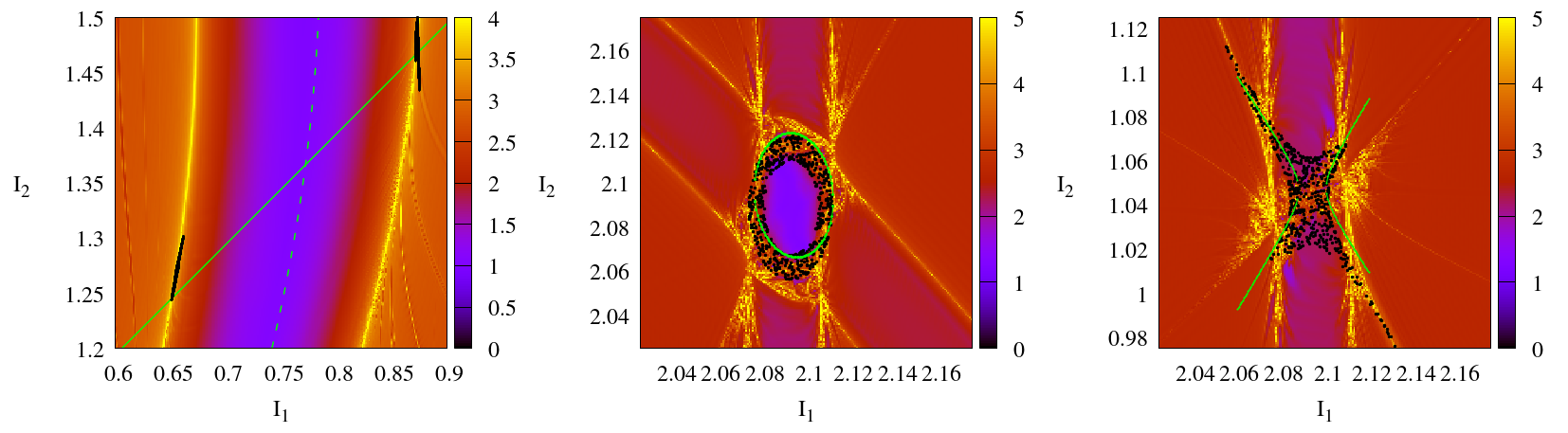
Figure 8: (a) Left: Arnold diffusion along a simple resonance in the model (20) for $\epsilon=0.1$ (see text). Center: Diffusion around the resonance junction A (quasi-convex domain). The ellipse represents the constant energy condition of Eq. (39). Right: Same as previously, but for the resonant junction B (non-convex, steep). The constant energy condition (39) now yields hyperbolas.

We mentioned in section 2 that it is possible to prove the existence of Arnold diffusion along the simple resonances of a priori stable systems (see CG). The first numerical example of Arnold diffusion in an a priori stable system similar to the one treated in the examples above (but with $H_{0}=(I_{1}^{2}+I_{2}^{2})+I_{3}$ satisfying everywhere the quasi-convexity condition) was provided by [44]. Several more examples, including a spectacular demonstration of the drift of the trajectories throughout the entire Arnold web, were provided in [37].

Figure 8 (left) gives an example of the slow drift along the resonance (1,1,0) in the model (20) around the point $I_{*}$ with $I_{1*}=0.77211...$, $I_{2*}=1.3665$, $I_{3*}=0$, for $\epsilon=0.1$. Using the FLI map, we first compute the borders of the resonance (yellow). We then compute the plane of fast drift crossing the chosen point $I_{*}$ (Eq. (29), thin line in Fig. 8). Computing the FLI (for $t=1000$) for initial conditions along this line, we obtain two points (on each separatrix layer) where the FLI has a local maximum. The point of maximum on the top right of the figure has co-ordinates $I_{1}=0.87166$, $I_{2}=1.466054$. Taking trajectories in a very small square (of size $10^{-5}$ in our case) around this point, and forward propagating these trajectories, allows to observe their slow drift along the separatrix layers of the resonance. The points in black in Fig. 8 correspond to only four such trajectories, integrated up to a time $t=10^{9}$. The trajectories are shown only when returning to the same angular section $(\phi_{1}+\phi_{2})\mod 2\pi=0$, and $\phi_{3}\mod 2\pi=0$ as the one for which the FLI was computed (with a numerical tolerance $10^{-2}$). We notice that the trajectories make an overall excursion in the action space of length $\sim 0.5$ after this long integration time. Due to the selected section, the trajectories yield points near the extrema of both branches of the theoretical separatrix of the resonance (see previous subsection), corresponding to the left and right groups of points in Fig. 8, which are both produced by the same trajectories. Besides the fast change in the resonant action $I_{R}$ (Eq. (3.2)), we observe that the trajectories undergo a slow change of the value of the adiabatic actions $I_{F1},I_{F2}$, a fact making them to jump from one to a nearby plane of fast drift, with all these planes parallel to the one shown in Fig. 8. How to quantify these jumps will be discussed in the next section.

The center and right panels of Fig. 8 refer now to chaotic trajectories around the resonant junctions A and B. We saw that the quadratic form of the constant energy condition of Eq. (39) yields ellipses in the case of the point A, while it yields hyperbolas in the case of the point B. Clearly, the chaotic trajectories around the junction are governed by this difference. In the case of the junction A, the normal form dynamics impedes the chaotic trajectories to move beyond a layer of thickness ${\cal O}(e)$ around each ellipse. In the case of the junction B, instead, the chaotic trajectories can have larger excursions by following a path close to the asymptotes of the hyperbolas. In that case, the trajectories are still limited around the resonant junction due to the cubic terms in the Hamiltonian (21).

On the other hand, all predictions made by the normal form models are valid up to an error determined by the exponentially small remainder of the normal form. More specifically, the Nekhoroshev normal form has the form:

$$H_{N}=Z_{N}+R_{N}$$ (41)

where $Z_{N}$ is the normal form part and $R_{N}$ the remainder, with

$$||R_{N}||={\cal O}\left(\exp((\epsilon_{0}/\epsilon)^{b})\right)~{}~{}.$$

Let $I_{Fi}$ (the ‘adiabatic actions’) be the integrals of $Z_{N}$ (in the 3DOF case, $i=1,2$ in the case of a simple resonance, and $i=1$ in the case of the double resonance). We have

$$\dot{I}_{Fi}=-\partial R_{N}/\partial\phi_{Fi},~{}~{}~{}i=1,2$$ (42)

For the derivatives we have the estimate $||\dot{I}_{F_{i}}||={\cal O}\left(\exp((\epsilon_{0}/\epsilon)^{b})\right)$. From this, we can conclude that, although the actions $I_{Fi}$ cease to be integrals of motion in the complete Hamiltonian, up to a given time $t$ the actions $I_{F_{i}}$ can have excursions of length bounded from above by $\Delta I_{F_{i}}<{\cal O}\left(t\exp((\epsilon_{0}/\epsilon)^{b})\right)$. This estimate yields the local speed of Arnold diffusion, which can hence be measured using the norm $||R_{N}||$. Another numerical test regards the comparison between the numerically computed (by ensembles of trajectories) value of the diffusion coefficient $D$, and the size of the remainder $||R_{N}||$. Empirical fitting has given the law $D\sim||R_{N}||^{3}$ in the case of simple resonances, and $D\sim||R_{N}||^{2}$ in the case of double resonances. Implementing the theory of Chirikov, instead, leads to the estimate $D\propto||R_{N}||^{2+\alpha}$, where the correction $0<\alpha<1$ depends locally (in a simply-resonant domain) on the detailed structure of the ‘layer resonances’ determining the remainder of the local Nekhoroshev normal form [14].

To unveil the detailed evolution of the variables $I_{F,i}(t)$ for any trajectory one needs to solve the initial value problem for the differential equations (41) up to any desired time $t$. It turns out that, even availing the explicit expressions for a high order truncation of the remainder $R_{N}$, in practice it is hard to try to integrate the differential equations (42) directly in the computer. A good number of reasons impede us on this task, starting from the fact that the remainder $R_{N}$ is actually a series, whose representation in the computer is given by a truncated trigonometric polynomial typically containing millions of terms. This is an expression hard to deal with not only numerically, but also in any theoretical attempt to establish the existence of phase space objects (e.g. manifolds like the ones of Fig. 5) having the role of drivers of Arnold diffusion.

On the other hand, we can always attempt to model the dynamics of itself the remainder $R_{N}$. As discussed in the sequel, such a modeling is possible and leads to a way more tractable expression $R_{N}^{(model)}$. Using $R_{N}^{(model)}$ we can then probe and visualize most phenomena related to Arnold diffusion. In particular, we can unravel the ‘jumps’ in action space (similar as in Fig. 1(d)) undergone by the weakly chaotic trajectories within the layers of a selected resonance. We can also predict and model the size of these jumps. Finally, we can identify the fastest drifting trajectories and monitor how close their speed is to the theoretical upper bound provided by the Nekhoroshev theorem $\Delta I_{F_{i}}(max)=t\sup_{{\cal D}_{*}}|\partial R_{N}/\partial\phi_{Fi}|$ (see examples in the next section).

4 Construction of the Nekhoroshev normal form: semi-analytical estimates

4.1 Construction of the Nekhoroshev normal form

It was mentioned before that most semi-analytical results on the quantification of the Arnold diffusion follow after the appropriate construction of a local Nekhoroshev normal form in a selected domain ${\cal D}_{*}$ around some point $I_{*}\in\mathbb{R}^{n}$ of the action space of the problem. We here summarize the method implemented in [24],[26],[14],[40], for an efficient computation of the Nekhoroshev normal form. We assume a n-DOF system with Hamiltonian

$$H(I,\phi)=H_{0}(I)+\epsilon H_{1}(I,\phi)~{}~{}~{},$$ (43)

satisfying the properties enumerated below.

4.1.1 Analyticity

We assume that there is an open domain ${\cal I}\subset\mathbb{R}^{3}$ and real constants $\rho>0,\sigma>0$ such that for all points $I_{*}\in{\cal I}$ and all complex quantities $J_{i}\in\mathbb{C}$, $i=1,\ldots n$ satisfying $|J_{i}|<\rho$ the following properties hold true:

i) the function $H_{0}$ can be expanded as a convergent Taylor series

$$H_{0}=H_{0*}+\omega_{*}\cdot J+{1\over 2}\sum_{i=1}^{n}\sum_{j=1}^{n}M_{ij*}J_{i}J_{j}+\ldots$$ (44)

where $\omega_{*}=\nabla_{I}H_{0}(I_{*})$ and $M_{ij*}$ are the elements of the Hessian matrix of $H_{0}$ at $I_{*}$, denoted by $M_{*}$.

ii) For all $I_{*}\in{\cal I}$, $H_{1}$ admits a Fourier expansion

$$H_{1}=\sum_{k}h_{k}(I_{*}+J)\exp(ik\cdot\phi)$$ (45)

analytic in the domain

$${\cal D}(I_{*})=\left\{I_{i}=I_{i*}+J_{i},|J_{i}|<\rho,\Re(\phi_{i})\in\mathbb{T},|\Im(\phi_{i})|<\sigma,i=1,\ldots n\right\}~{}~{}.$$ (46)

The analyticity of the function $H_{1}$ in the domain ${\cal D}$ implies that all the coefficients $h_{k}$ can be expanded in convergent Taylor series around $I_{*}$ as

$$h_{k}=h_{k*}+\nabla_{I_{*}}h_{k}\cdot J+{1\over 2}\sum_{i=1}^{n}\sum_{j=1}^{n}h_{k,ij*}J_{i}J_{j}+\ldots$$ (47)

4.1.2 Book-keeping

Due to the analyticity of $H_{1}$, the Fourier coefficients $h_{k}$ in the domain ${\cal D}(I_{*})$ decay exponentially, that is, there are positive constants $A$, $\sigma$ such that

$$\sup_{\cal D_{*}}|h_{k}(I)|<Ae^{-|k|\sigma}$$ (48)

Taking the exponential decay into account, we then split the Fourier harmonics in groups with the wave number satisfying $(s-1)\leq|k|<sK-1$, $s=1,2,\ldots$, and

$$K=-{1\over\sigma}\log(\rho_{0})~{}~{},$$ (49)

where $\rho_{0}$ is the size of the domain around the point $I_{*}$ where the normal form is to be computed, i.e., $|J_{i}|<\rho_{0}$. For resonant constructions of any multiplicity it is convenient to take $\rho_{0}={\cal O}(\sqrt{\epsilon})$. Introducing a ‘book-keeping’ symbol $\lambda$, with numerical value $\lambda=1$, the Hamiltonian can then be split in ascending powers of $\lambda$:

$$H=H^{(0)}(J,\phi) = Z_{0}+\sum_{s=1}^{\infty}\lambda^{s}H^{(0)}_{s}(J,\phi;\epsilon)$$ (50)

where

$$Z_{0}=\omega_{*}\cdot J$$

and

$$H^{(0)}_{s}=\sum_{\mu=1}^{s}\sum_{k=K^{\prime}(s-\mu)}^{K^{\prime}(s-\mu+1)-1}H^{(0)}_{\mu,k}(J)\exp(ik\cdot\phi)$$ (51)

where $H^{(0)}_{\mu,k}(J)$ are polynomials containing terms of degree $\mu-1$ or $\mu$ in the action variables $J$. In the $n=3$ cases dealt with in the numerical examples of this article, we have, in particular:

$$H^{(0)}_{\mu,k}(J)=\epsilon\sum_{\mu_{1}=0}^{\mu-1}~{}~{}\sum_{\mu_{2}=0}^{\mu-1-\mu_{1}}~{}~{}\sum_{\mu_{3}=0}^{\mu-1-\mu_{1}-\mu_{2}}{1\over\mu_{1}!\mu_{2}!\mu_{3}!}{\partial^{\mu-1}h_{1,k}(I_{*})\over\partial^{\mu_{1}}I_{1}\partial^{\mu_{2}}I_{2}\partial^{\mu_{3}}I_{3}}J_{1}^{\mu_{1}}J_{2}^{\mu_{2}}J_{3}^{\mu_{3}}$$

if $|k|>0$, or

$$H^{(0)}_{\mu,k}(J)=\sum_{\mu_{1}=0}^{\mu}~{}~{}\sum_{\mu_{2}=0}^{\mu-\mu_{1}}~{}~{}\sum_{\mu_{3}=0}^{\mu-\mu_{1}-\mu_{2}}{1\over\mu_{1}!\mu_{2}!\mu_{3}!}{\partial^{\mu}H_{0}(I_{*})\over\partial^{\mu_{1}}I_{1}\partial^{\mu_{2}}I_{2}\partial^{\mu_{3}}I_{3}}J_{1}^{\mu_{1}}J_{2}^{\mu_{2}}J_{3}^{\mu_{3}}$$

$$~{}~{}~{}~{}~{}~{}~{}~{}+\epsilon\sum_{\mu_{1}=0}^{\mu-1}~{}~{}\sum_{\mu_{2}=0}^{\mu-1-\mu_{1}}~{}~{}\sum_{\mu_{3}=0}^{\mu-1-\mu_{1}-\mu_{2}}{1\over\mu_{1}!\mu_{2}!\mu_{3}!}{\partial^{\mu-1}h_{1,0}(I_{*})\over\partial^{\mu_{1}}I_{1}\partial^{\mu_{2}}I_{2}\partial^{\mu_{3}}I_{3}}J_{1}^{\mu_{1}}J_{2}^{\mu_{2}}J_{3}^{\mu_{3}}$$

if $k=0$. In all the above expressions, the superscript $(0)$ means ‘the starting Hamiltonian of the iterative normalization process’. This is simply the original Hamiltonian re-organized in powers of the book-keeping symbol $\lambda$. Subscripts (as e.g. $s$ in the functions $H^{(0)}_{s}(J,\phi;\epsilon)$) mean terms book-kept with the power $\lambda^{s}$. In physical terms, this can be interpreted as ‘terms of the s-th order of smallness’. All expressions in the initial and in subsequent normalization steps are finite, i.e., they are trigonometric polynomials easily represented in the computer’s memory via an indexing function. The maximum ‘book-keeping’ order $N_{tr}$ adopted in the normalization algorithm is called the truncation order.

4.1.3 Resonant module

Following the definitions given in subsection 4.2, the point $I_{*}$, and its corresponding frequency vector $\omega_{*}=\omega(I_{*})$, are called ‘$M-$tuple resonant’ (with $0\leq M\leq n-1$) if there can be found $M$ linearly independent non-zero integer vectors $k^{(i)}$, $i=1,\ldots M$ such that $k^{(i)}\cdot\omega_{*}=k^{(i)}\cdot\omega(I_{*})=0$ for all $i=1,\ldots,M$. When a point $I_{*}$ is $M-$tuple resonant, there are many harmonics $\cos(k\cdot\phi)$ with $|k|\neq 0$ in the Hamiltonian which cannot be normalized since their elimination would involve a divisor exactly equal to zero. The set of all possible wavevectors $k$ such that $k\cdot\omega_{*}=0$ is called the resonant module at the point $I_{*}$. Since checking numerically the condition $k\cdot\omega_{*}=0$, with $\omega_{*}\in\mathbb{R}^{n}$, is sensitive to round-off errors, a convenient way to define the resonant module, which involves only operations among integer numbers, is by use of the concept of ‘pseudo-frequency’ vector. This is defined as follows: if $\omega_{*}$ is $M-$tuple resonant with $M\geq 1$, choose $M$ non-zero linearly independent integer vectors $k^{(i)}$, $i=1,\ldots,M$ such that $k^{(i)}\cdot\omega(I_{*})=0$. Then, there exist $n-M$ non-zero integer vectors $m^{(j)}$, $j=1,\ldots,n-M$ such that $k^{(i)}\cdot m^{(j)}=0$ for all possible pairs $i,j$. To define these vectors, solve the $n-M$ systems of linear equations given by

$$k^{(1)}_{1}q_{1}^{(j)}+k^{(1)}_{2}q_{2}^{(j)}+\ldots+k^{(1)}_{M}q_{M}^{(j)}=-k^{(1)}_{M+j}$$

$$k^{(2)}_{1}q_{1}^{(j)}+k^{(2)}_{2}q_{2}^{(j)}+\ldots+k^{(2)}_{M}q_{M}^{(j)}=-k^{(2)}_{M+j}$$

$$\ldots$$

$$k^{(M)}_{1}q_{1}^{(j)}+k^{(M)}_{2}q_{2}^{(j)}+\ldots+k^{(M)}_{M}q_{M}^{(j)}=-k^{(M)}_{M+j}$$

for $j=1,\ldots,n-M$. The solutions give vectors $q^{(j)}=(q_{1}^{(j)},\ldots,q_{M}^{(j)},\delta_{M+1,M+j},\ldots,\delta_{n,M+j})$ with rational components. Multiplying the vector $q^{(j)}$ with the maximal common divisor of all its components yields the j-th pseudo-frequency vector $m^{(j)}$.

We can now determine which harmonics $\cos(k\cdot\phi)$ to be excluded from the normalization process. The set of all integer vectors $k$ corresponding to the excluded harmonics is called the resonant module ${\cal M}(k^{(1)},\ldots,k^{(M)})$ defined as:

$${\cal M}(k^{(1)},\ldots,k^{(M)})=\left\{\begin{array}[]{ll}\{k=(0,0,\ldots,0)\}&~{}~{}\mbox{if}~{}M=0\\ \{k\in\mathbb{Z}^{n}:k\cdot m^{(j)}=0~{}~{}~{}\mbox{for all}~{}j=1,\ldots,n-M\}&~{}~{}\mbox{if}~{}M>0\end{array}\right.$$ (53)

where $m^{(j)}$, $j=1,\ldots,n-M$ are the pseudo-frequency vectors determined through Eq.(4.1.3).

Note that, even when the origin of the expansion $I_{*}$ is non-resonant, i.e., when $M=0$, arbitrarily close to it there can be found $M-$tuple resonant points of any multiplicity $M>0$. This is a consequence of the fact that resonances are dense in the action space (see the examples in [25]). Whenever the non-resonant vector $\omega_{*}$ is ‘close’ to a low-order M-tuple resonant vector $\Omega$, in the sense that $|\omega_{*}-\Omega|<\alpha$ with $\alpha$ small, and the wavevectors $k$ satisfying $k\cdot\Omega$ are of order $|k|$ smaller than the ‘cut-off’ order (see below), we say to be in a ‘near-resonance’ case. In this case too, we may wish to avoid the presence in the series of those divisors $k\cdot\omega_{*}$ for which $k\cdot\Omega=0$. We then define the resonant module as above, but using $\Omega$ in the place of $\omega_{*}$.

4.1.4 Hamiltonian normalization

We consider a sequence of normalizing canonical transformations

$$(\phi,J)\equiv(\phi^{(0)},J^{(0)})\rightarrow(\phi^{(1)},J^{(1)})\rightarrow(\phi^{(2)},J^{(2)})\rightarrow\ldots$$

leading to re-express the Hamiltonian, after $r$ normalization steps, in new canonical variables $(\phi^{(r)},J^{(r)})$ such that

$$H(\phi((\phi^{(r)},J^{(r)}))=Z^{(r)}((\phi^{(r)},J^{(r)});\lambda,\epsilon)+R^{(r)}(\phi^{(r)},J^{(r)};\lambda,\epsilon)~{}~{}.$$ (54)

The functions $Z^{(r)}(J^{(r)},\phi^{(r)};\lambda,\epsilon)$ and $R^{(r)}(J^{(r)},\phi^{(r)};\lambda,\epsilon)$ are called the normal form and the remainder respectively. The normal form is a finite expression which contains terms up to order $r$ in the book-keeping parameter $\lambda$. By definition, these are terms belonging to the resonant module ${\cal M}(k^{(1)},\ldots,k^{(M)})$. The remainder, instead, is a convergent series containing terms of order $\lambda^{r+1}$, including all possible harmonics.

To compute the normalizing transformation, we use the composition of Lie series with generating functions $\chi_{1},\ldots,\chi_{r}$. Denote $Q=(\phi,J)\equiv Q^{(0)}$. The normalizing transformation is:

$$Q^{(r)}=\exp(-L_{\chi_{1}})\exp(-L_{\chi_{2}})\ldots\exp(-L_{\chi_{r}})Q\\$$ (55)

The generating functions are determined recursively, by solving, for
$n_{r}=0,\ldots,r-1$ the homological equations:

$$\{\omega_{*}\cdot J^{(n_{r}+1)},\chi_{n_{r}+1}\}+\lambda^{n_{r}+1}\tilde{H}^{(n_{r})}_{n_{r}+1}(J^{(n_{r}+1)},\phi^{(n_{r}+1)})=0$$ (56)

where

$$H^{(n_{r})}=\exp(L_{\chi_{n_{r}}})H^{(n_{r}-1)}~{}~{}.$$ (57)

4.1.5 Optimal remainder

Basic normal form theory (see [25]) establishes that the above normalization process has an asymptotic character. Namely, i) the domain of convergence of the remainder series $R^{(r)}$ shrinks as the normalization order $r$ increases, and ii) the size $||R^{(r)}||$ of $R^{(r)}$, where $||\cdot||$ is a properly defined norm in the space of trigonometric polynomials, initially decreases, as $r$ increases, up to an optimal order $r_{opt}$ beyond which $||R^{(r)}||$ increases with $r$. In the Nekhoroshev regime, one has $||Z^{(r_{opt})}||>>||R^{(r_{opt})}||$. Hence, the normal form obtained at the order $r_{opt}$ best unravels the dynamics, which is given essentially by the Hamiltonian flow of $Z^{(r_{opt})}$ slightly perturbed by $R^{(r_{opt})}$. Furthermore, the optimal normalization order $r_{opt}$ depends on $\epsilon$ via an inverse power-law ([24][26]), namely

$$r_{opt}\sim\epsilon^{-a}~{}~{},$$ (58)

for some positive exponent $a$ depending on the multiplicity of the resonance around which the normal form is computed. The leading terms in the optimal remainder function are $O(\lambda^{r_{opt}+1})$. Due to the book-keeping relation (49), the terms of order $\lambda^{r_{opt}}$ have size estimated as $e^{-\sigma K_{opt}}$, where

$$K_{opt}(\epsilon)=K^{\prime}r_{opt}(\epsilon)$$ (59)

is called the Nekhoroshev cut-off order. Then, $K_{opt}\sim K^{\prime}\epsilon^{-a}$, implying:

$$||R^{(r_{opt})}||\sim\epsilon^{1/2}\exp\left({-K^{\prime}\sigma\over\epsilon^{a}}\right)$$ (60)

i.e., the remainder at the optimal normalization order is exponentially small in $1/\epsilon$.

In practice, to specify the optimal normalization order, after performing all the above symbolic computations with the aid of a computer program, we proceed as follows: we set the truncation order $N_{t}$ to be several orders larger than the maximum reached normalization order $r$. Then, we compute the truncated-norm estimates

$$||R^{(r)}||_{W^{(r)}}=\sum_{s=r+1}^{N_{t}}\sum_{m}\sup|R^{(r)}_{s}|_{W^{(r)}}$$ (61)

where $\sup|R^{(r)}_{s}|$ means the sup norm of the s-th book-keeping term of the truncated remainder over a domain of interest $Q^{(r)}\in W^{(r)}$ where the r-th step canonical variables. To this end, we first probe numerically that $W^{(r)}$ is smaller than the convergence domain for the r-th step normalization. We then verify the asymptotic character of the sequence $||R^{(r)}||_{W^{(r)}}$, for $r=1,2,3,\ldots$. That is, for $\epsilon$ sufficiently small, initially (at low orders) $||R^{(r)}||_{W^{(r)}}$ decreases as $r$ increases, up to the optimal order $r_{opt}$ at which $||R^{(r_{opt})}||_{W^{(r_{opt})}}$ reaches a minimum. Then, for $r>r_{opt}$, $||R^{(r)}||_{W^{(r)}}$ increases with $r$. This behavior is exemplified in Fig.9, referring to the normal form computed for the data of the simple resonance corresponding to the left panel of Fig. 8.

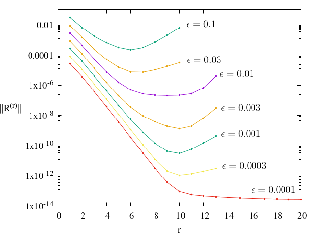
Figure 9: Size of the remainder as a function of the normalization order $r$ for various values of $\epsilon$. The value of $r$ at the minimum of each curve corresponds to the optimal normalization order. Note that the optimal order is higher than 20 in the case $\epsilon=0.0001$.

4.2 Removal of deformation effects

We have seen that, at the optimal order, the adiabatic actions $I^{(r_{opt})}_{Fi}$ are integrals of the normal form dynamics, while in the full Hamiltonian they undergo exponentially small time variations due to the exponentially small optimal remainder. One important effect, which impedes to measure the real speed of the variations of the adiabatic action variables is deformation. Consider the inverse of the transformation (55) at optimal order:

$$Q=\exp(L_{\chi_{r}})\exp(L_{\chi_{r-1}})\ldots\exp(L_{\chi_{1}})Q^{(r_{opt})}\\$$ (62)

Due to the relation $\exp(L_{\chi_{1}})Q^{(r_{opt})}=Q^{(r_{opt})}+\{Q^{(r_{opt})},\chi_{1}\}+\ldots$, as well as the fact that $\chi_{s}={\cal O}(\rho_{0}^{s})$, we have that

$$Q=Q^{(r_{opt})}+{\cal O}(\rho_{0})$$ (63)

Furthermore, for resonant normal forms, we saw that $\rho_{0}={\cal O}(\epsilon^{1/2})$. Thus, we find that even while the adiabatic actions $I^{(r_{opt})}_{Fi}$ undergo a very slow time variation (including drift), in the original variables this variation is completely hidden in a ${\cal O}(\epsilon^{1/2})$ oscillation, due entirely to the canonical transformation linking old with new variables. Since, without knowledge of the normalizing transformation, we are forced to deduce all the information on the behavior of the system by numerical experiments performed using the original variables, this implies that we have to recover the drift by removing all the noise induced by these large amplitude, but irrelevant for dynamics, oscillations.

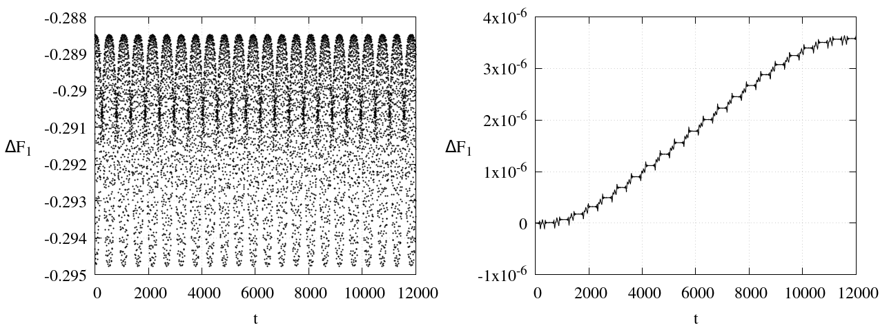
Figure 10: Evolution of the adiabatic action $J_{F}$ along a simple resonance in the model (20). Left: numerical trajectory. Right:, the same trajectory, but plotted in the optimal canonical variable $J_{F}^{(r_{opt})}$ (see text).

Being able to compute the optimal normalizing transformation, allows, instead to spectacularly remove the deformation effect and easily obtain (and measure) the underlying drift of the adiabatic action variables. Figure 10 shows the removal of the deformation in the case of a trajectory undergoing Arnold diffusion in the model (20) and with initial condition as in Fig. 8. Recall that to visualize the drift using the original variables in that case has required an extremely long integration time $t=10^{9}$. For quite shorter times, instead, ($t=10^{4}$ in Fig. 10) the drift of the unique adiabatic action of the problem, measured by $\Delta{F,1}=I_{F}(t)-I_{F}(0)$ is completely hidden in a oscillation of size $~{}0.2$ (Fig. 10, left), and thus impossible to measure with numerical experiments up to the time $t=10^{4}$. If, instead, we pass all the numerical data $Q(t)$ of the trajectory through the optimal normalizing transformation (Eq. (55)), we obtain the evolution of the optimal variable $\Delta{F,1}^{(r_{opt})}=I_{F}^{(r_{opt})}(t)-I_{F}^{(r_{opt})}(0)$, shown in Fig. 10, right. Now, the drift is clearly demonstrated, and its local velocity can be measured by a simple fitting to the data. In fact, as discussed in the next subsection, the drift in the action space is not necessarily monotone, and $\Delta{F,1}^{(r_{opt})}(t)$ may exhibit both an increase or decrease at different intervals of time. At any rate, the ability to remove the deformation effect can be exploited in the modeling of the evolution of the adiabatic action variables, as discussed in the next subsection.

4.3 Modeling the jumps in the adiabatic action variables

We have mentioned that it is possible to prove the occurrence of the Arnold mechanism in a priori stable systems only in the case of simple resonances (CG). We will now discuss how to model the evolution of the adiabatic action variables, including the jumps similar in nature as those of the original Arnold model, using, however, the information encapsulated in the remainder at the optimal normalization order. Consider an optimal Hamiltonian of the form (54) obtained by normalization around a simply-resonant point $I_{*}$.

Following [40], to simplify all notations, denote as $H^{N}$ (the ‘Nekhoroshev normal form’) the Hamiltonian $H^{(r_{opt})}$, depending on the resonant action-angle variables $(S,\sigma)\equiv\left(J_{R}^{(r_{opt})},\phi_{R}^{(r_{opt})}\right)$ and the $n-1$ adiabatic action variables conjugate to fast angles $(F,\phi)\equiv\left(J_{F}^{(r_{opt})},\phi_{F}^{(r_{opt})}\right)$ (see section 3). With the new notation, we have

$$H^{N}=h(F,S)+\epsilon f^{N}(F,S,\sigma)+r^{N}(F,S,\sigma,\phi)~{}~{}~{}.$$ (64)

The (simply-resonant) normal form is

$$\overline{H}^{N}=h(F,S)+\epsilon f^{N}(F,S,\sigma)~{}.$$ (65)

The remainder $r^{N}$ is provided as a Taylor-Fourier series:

$$r^{N}=\sum_{m\geq 0}\sum_{\nu\in{\mathbb{Z}}^{d}}\sum_{k\in{\mathbb{Z}}^{n-d}}r^{m}_{\nu,k}(F)(S-S_{*})^{m}e^{i\nu\cdot\sigma+ik\cdot\phi}$$ (66)

expanded at a suitable $S_{*}$, with computer-evaluated truncations involving a large number (typically $10^{7}$ to $10^{8}$) terms.

To define the resonant normal form dynamics, as in section 3 we first expand $\overline{H}^{N}$ at the values of the actions $(F_{*},S_{*})$ identifying the center of the resonance, where

$${\partial h\over\partial S}(S_{*},F_{*})=0,$$ (67)

Then

$$\overline{H}=\overline{H}_{0}+...\ \ ,\ \ \overline{H}_{0}=\omega_{*}\cdot\hat{F}+{A\over 2}\hat{S}^{2}+\hat{S}B\cdot\hat{F}+{1\over 2}C\hat{F}\cdot\hat{F}+\epsilon v(\sigma)$$ (68)

where $\hat{F}=F-F_{*}$, $\hat{S}=S-S_{*}$, $A\in{\mathbb{R}}$, $\omega_{*},B\in{\mathbb{R}}^{n-1}$, $C$ is a $(n-1)\times(n-1)$ square matrix and $v(\sigma)$ is a trigonometric function depending parametrically on $S_{*}(I_{*}),F_{*}(I_{*})$. The actions $\hat{F}$ are the constants of motion for the Hamiltonian flow of $\overline{H}_{0}$.

Consider, now, the family of curves $\hat{S}(u;\alpha)$, for different $a$, given by

$$\hat{S}=\sqrt{\epsilon}s_{\alpha}(\sigma)=\pm\sqrt{\epsilon}\sqrt{{2\over|A|}(M(1+\alpha)-v(\sigma))}$$ (69)

where $M=\max_{\sigma\in[0,2\pi]}v(\sigma)$, and $\alpha$ is the energy of the pendulum Hamiltonian (equal to $\overline{H}_{0}$ for $\hat{F}=0$):

$$a={A\over 2}\hat{S}^{2}+\epsilon v(\sigma)=\epsilon M(1+\alpha)~{}~{}.$$ (70)

Since $\overline{H}_{0}$ has the structure of a pendulum Hamiltonian, we can attempt to implement the Melnikov approximation, introduced in section 2, in order to compute the jumps in the variables $F$ over one complete homoclinic transition of the variables $(\hat{S},\sigma)$, assigning to the remainder $r^{N}$ (Eq. (66)) the role of the coupling term between the resonant variables $(S,\sigma)$ and the remaining variables $(F,\phi)$. Since $\dot{F_{j}}=-\partial r^{N}/\partial\phi_{j}$, the Melnikov approximation will then consist of estimating the variation $\Delta F_{j}(T)=F_{j}(t)-F_{j}(0)$ after a time $T$ via the integral

$$\Delta F_{j}(T)=-\sum_{m,\nu,k}\int_{0}^{T}ik_{j}r^{m}_{\nu,k}(F(t))\hat{S}(t)^{m}e^{i\nu\sigma(t)+ik\cdot\phi(t)}dt:=\sum_{m,\nu,k}\Delta F_{j,T}^{m,\nu,k}~{}~{}.$$ (71)

where the true solution $(F(t),S(t),\sigma(t),\phi(t))$ in the r.h.s of the integrals (71) will be substituted by the approximate solution under the flow of the normal form $\overline{H}_{0}$

$$(F_{*},S^{0}(t),\sigma^{0}(t),\phi^{0}(t))=(F_{*},S_{*},0,0)+(0,\hat{S}^{0}(t),\sigma^{0}(t),\phi^{0}(t))$$

where $(0,\hat{S}^{0}(t),\sigma^{0}(t),\phi^{0}(t))$ is a solution of Hamilton’s equations of $\overline{H}_{0}$.

Contrary to the simple model of section 2, it is important to recall that the number of Melnikov integrals to compute in (71) are of the same order as the number of remainder terms ($10^{7}$ to $10^{8}$), thus the computation is hardly tractable in practice. However, we get an enormous simplification of the problem noticing that, out of all these integrals, only few ($\sim 10^{3}$) really contribute to the result. To this end, we first observe that representing $\hat{S}^{0}(t)$ parametrically as a function of $\sigma^{0}(t)$, for fixed $\alpha$, allows to change the integration variable in (71) from $t$ to $\sigma$:

$$\Delta F_{j,T}^{m,\nu,k}(T)\simeq\Delta^{0}F_{j,T}^{m,\nu,k}(T)\hskip-5.69046pt=-ik_{j}{{r^{m}_{\nu,k}(F_{*})\epsilon^{m-1\over 2}\over A}e^{ik\cdot\phi(0)}}\hskip-5.69046pt\int_{0}^{\sigma^{0}(T)}\hskip-17.07182pt[s_{\alpha}(\sigma)]^{m-1}e^{i\theta(\sigma)}d\sigma$$ (72)

where the phase $\theta(\sigma)$ is defined by:

$$\theta(\sigma)={{\cal N}\sigma+{\Omega\over A\sqrt{\epsilon}}\int_{0}^{\sigma}{dx\over s_{\alpha}(x)}}$$

with

$${\cal N}=\nu+k\cdot B/A,~{}~{}~{}~{}\Omega=k\cdot\omega_{*}~{}~{}~{}.$$ (73)

Then, invoking the principle of stationary phase, it is clear that only integrals involving a slow variation of the phase $\theta(\sigma)$ over a time $T_{\alpha}$, representing the period of one homoclinic transition, will be important in the computation of the jumps via the Eq. (72).

To make this argument more explicit, assume that the lowermost order terms in the resonant normal form (for $\hat{F}=0$) have the form of the pendulum Hamiltonian:

$$H_{pend}={|A|\over 2}{\hat{S}}^{2}+\epsilon\beta\cos\sigma+...$$ (74)

where, for simplicity, we set $\epsilon,\beta>0$. Consider a remainder term labeled by the integers $(m,\nu,k)$ in Eq. (72). Using the approximation (74), and setting $\alpha=0$ (separatrix solution), the function $\theta(\sigma)$ for the term in question can be approximated by:

$$\theta(\sigma)\approx\theta_{0}+{\cal N}\sigma+{\cal W}\ln\tan(\sigma/4),~{}~{}~{}{\cal W}={\Omega\over\sqrt{|A|\beta\epsilon}}~{}~{}.$$ (75)

where ${\cal N}$ and $\Omega$ are given by Eq. (73), hence, they depend only on the term labels $\nu,k$. From Eq. (75), we obtain

$$\theta^{\prime}(\sigma)\approx{\cal N}+\frac{{\cal W}}{2}\frac{1}{\sin(\sigma/2)}$$ (76)

Therefore, one has $\lim_{\sigma\rightarrow 0}W\theta^{\prime}(\sigma)=\lim_{\sigma\rightarrow 2\pi}W\theta^{\prime}(\sigma)=+\infty$, and since $\theta^{\prime}(\sigma)$ is a function symmetric with respect to $\pi$ and monotonically decreasing (increasing) in $[0,\pi)$ ($(\pi,2\pi]$), there exists a minimum of the function at $\sigma=\pi$ of value $\theta^{\prime}(\sigma)={\cal N}+{\cal W}/2$. Thus, $\theta^{\prime}(\sigma)$ has zeroes (stationary points) $\sigma_{c}=\pi\pm\Delta\sigma_{c}$, with $0<\Delta\sigma_{c}<\pi$, if and only if the minimum value $\theta^{\prime}(\pi)$ is negative. This lead to the following condition:

$$\mathrm{The\,\,term\,\,defined\,\,by\,\,}(m,\nu,k)\mathrm{\,\,is\,\,stationary}\iff{\cal N}\cdot{\cal W}<0\,\,\mathrm{and}\,\,|{\cal N}|>{|{\cal W}|\over 2}$$ (77)

In case the condition (77) is not satisfied, we still have to check for the existence of terms $(m,\nu,k)$ which, albeit non-stationary, exhibit only a small variation of the phase $\theta(\sigma)$ over the period of the homoclinic transition. Such terms will be called quasi-stationary and they can be selected from the remainder by the following procedure: neglecting the slowly varying factor $[s_{a}(\sigma)]^{m-1}$ in Eq. (72), and factoring out a constant phase $e^{i(\theta_{0}+{\cal N}\pi)}$, important quasi-stationary terms are those for which the integral

$$\Delta{\cal I}=\int_{0}^{2\pi}\cos\left({\cal N}(\sigma-\pi)+{\cal W}\ln\tan(\sigma/4)\right)$$ (78)

has absolute value above a small (arbitrarily chosen) threshold $\mu_{0}$. Consider for a moment the approximation ${\cal W}\simeq const.$. Since the inspected term is assumed not to be stationary (not selected by the condition (77)), we have that ${\cal N}$ varies according to ${\cal N}\geq-{\cal W}/2$ for ${\cal W}>0$, or ${\cal N}\leq-{\cal W}/2$ for ${\cal W}<0$. Different values of ${\cal N}$ generate different behaviors for $\theta(\sigma)$, symmetric with respect to $\sigma=\pi$, as shown in Fig. 11(a). Figure 11(b) shows the functions $\cos\left({\cal N}(\sigma-\pi)+{\cal W}\ln\tan(\sigma/4)\right)$, for the same frequencies $\sigma$ of panel (a). From the comparison of the two plots, we see that the nearly flat domains of the curve $\theta(\sigma)$ near $\sigma=\pi$, along with the sigmoid variations at the two ends (in panel (a)) imply the formation of a plateau of the curves in (b) accompanied by fast lopsided oscillations, which nearly cancel each other in the integral (78). The flatter the function $\theta(\sigma)$ in the vicinity of $\sigma=\pi$, the wider is the plateau of $\cos(\theta(\sigma))$. Since the dominant contribution in $\Delta{\cal I}$ comes from the central plateau of $\cos(\theta(\sigma))$, the maximum absolute value of $\Delta{\cal I}$ occurs when the slope $\theta^{\prime}(\sigma)$ becomes zero at $\sigma=\pi$. Hence, from Eq. (76), the maximum occurs when ${\cal N}=-{\cal W}/2$. The length of the plateau is given by $\Delta\sigma_{p}=2\sigma_{p}$, where $\theta(\pi\pm\sigma_{p})=\pi/2$. From Eq. (75), we find $\sigma_{p}\simeq(24\pi/{\cal W})^{1/3}$, and hence $\Delta{\cal I}_{{\cal N}=-{\cal W}/2}\propto{\cal W}^{-1/3}$, an estimate verified numerically (Fig. 11(e)).

On the other hand, if ${\cal N}$ is ‘detuned’ from the maximum value $-{\cal W}/2$, the associated plateaus attenuate, leading to a decrease of $\Delta{\cal I}$. Yet, some of these contributions can be larger than minimum threshold considered for Eq. (78). Setting ${\cal N}=(\delta-1){\cal W}/2$, Fig. 11(f) shows the attenuation as function of the detuning $\delta$ for fixed ${\cal W}$. For small $\delta$, the attenuation is nearly a linear function of $\delta$ with negative slope, $\Delta{\cal I}\propto\Delta\sigma_{p}\approx(24\pi)^{1/3}{\cal W}^{-1/3}-(64/3\pi)^{1/3}{\cal W}^{1/3}\delta$. If we extend the straight line with negative slope in Fig. 11(f) up to the point where the line intersects the axis $\Delta I=0$ we find a critical detuning $\delta_{c}\approx(3\pi/2\sqrt{2})^{2/3}{\cal W}^{-2/3}$ beyond which the term can no longer be characterized as quasi-stationary. Actually, $\delta_{c}$ computed as above underestimates the true value of the detuning, since (i) the curve $\Delta{\cal I}$ has a tail extending only asymptotically to zero (i.e. as small as it may be, the contribution of a quasi-stationary terms is never exactly zero) and (ii) the slope found by linear fitting of the left part of the curves $\Delta I$ vs. $\delta$ for various values of ${\cal W}$ shows that the power law estimate of the slope $\propto{\cal W}^{p}$ yields an exponent substantially larger than $1/3$ for values of ${\cal W}$ well below unity (Fig. 11(g)). On the other hand, a numerical evaluation of the dependence of the critical detuning $\delta_{c}$ as function of ${\cal W}$ (Fig. 11(h)) yields a law $\delta_{c}\propto{\cal W}^{-q}$, with $q\approx 0.8$, i.e., slightly larger than the theoretical estimate $q=2/3$. Taking into account all these considerations, we formulate a heuristic criterion for quasi-stationarity, namely:

$$\mathrm{The\,\,term\,\,defined\,\,by\,\,}(m,\nu,k)\mathrm{\,\,is\,\,quasi-stationary\,\,\,}$$

$$\iff{\cal N}\cdot{\cal W}<0\,\,\mathrm{and}\,\,|{\cal N}|<(1-\delta_{c}){|{\cal W}|\over 2}$$

with $\delta_{c}=\delta_{c0}|{\cal W}|^{-0.8}$, where, by numerical fitting, $\delta_{c0}\simeq 3$ for an adopted attenuation factor $0.1$, or $\delta_{c0}=4.2$ for an adopted attenuation factor $\sim 0.01$.

Figure 11: (a) The function $\theta(\sigma)$ (equation 75) written as $\theta(\sigma)={\cal W}[0.5(1-\delta)](\sigma-\pi)+\ln\tan(\sigma/4))$ for ${\cal W}=1$ and $\delta=0$ (thick blue), $\delta=1$ (dashed green), or $\delta=2$ (thin red). The corresponding curves $\cos(\theta(\sigma)$ are shown in (b). The extent of the ‘plateau’ is reduced for larger $\delta$. Similar curves are shown in (c) and (d) for ${\cal W}=10$, and $\delta=0$, $0.1$ and $0.5$. (e), the integral $\Delta I$ (equation 78) for $\delta=0$, as a function of $|{\cal W}|$. (f) The attenuation of the integral $\Delta I$ with respect to its value for $\delta=0$ as $\delta$ increases, for fixed ${\cal W}=10$. The linear part of the curve, for small $\delta$ can be fitted with a line of negative slope $Q_{\delta}$. (g) The slope $|Q_{\delta}|$ as a function of $|{\cal W}|$. (h) The critical value $\delta_{c}$ for which the integral $\Delta I$ attenuates to $10\%$ its value at $\delta=0$, as a function of $|{\cal W}|$.

The conditions (77) and (4.3) are derived by considering the upper branch of the separatrix solution $\theta(\sigma)$. For the lower branch we have, instead, $\theta(\sigma)={\cal N}\sigma-{\cal W}\ln\tan(\sigma/4)$, hence we obtain the same conditions for stationary of quasi-stationary terms, but with the inequality ${\cal N}\cdot{\cal W}>0$ instead of ${\cal N}\cdot{\cal W}<0$. Also, the above analysis, based solely on the behavior of the phase $\theta(\sigma)$, allows to identify stationary or quasi-stationary terms for $|{\cal W}|$ arbitrarily large. It is important to recognize that the quantity $\Omega=k.\omega_{*}={\cal W}(|A|\beta\epsilon)^{1/2}$, represents the divisor associated with the remainder term $(m,\nu,k)$. Thus, we may further restrict the selection of remainder terms by retaining only those passing the stationary or quasi-stationary criterion, and simultaneously satisfying an upper threshold for the divisor value, say $|\Omega|<1$.

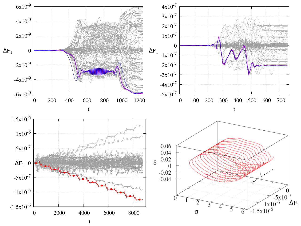
Figure 12: Top: Evolution of $F_{1}(t)$ for a swarm of 100 trajectories with initial conditions very close to the hyperbolic torus at the simply resonant point $I_{*}$ same as in Fig.8, but for $\epsilon=0.003$ (left) or $\epsilon=0.01$ (right). The blue curves show the fitting to one trajectory of the swarm using the Melnikov integrals (71) for only those remainder terms selected as stationary or quasi-stationary. Bottom: A ballistic orbit, drifting continuously in the same direction along the resonance, as depicted for the evolution $F_{1}(t)$ (left) or $F_{1}\times$ the pendulum variables $S,\sigma$ (right).

Figure 12 shows the main result obtained by selecting only the few terms ($\sim 1000$) of the remainder passing the criteria of stationarity or quasi-stationarity. Swarms of 100 trajectories with initial conditions very close to the hyperbolic torus at the simply resonant point $I_{*}$ same as in Fig. 8, but for $\epsilon=0.003$ (top left) or $\epsilon=0.01$ (top right) for a very small time ($T=1200$ and $T=700$ respectively), corresponding to the time required for the orbits to complete the first homoclinic transition along the pendulum, according to the approximative formula:

$$T_{\alpha}={1\over\sqrt{A\epsilon\beta}}\ln(32A\epsilon\beta/||R^{opt}||)~{}$$ (80)

This formula is the same as Eq. (11) used in section 2, setting the pendulum energy as $\varepsilon=A\epsilon\beta$, with the coefficients $A$ and $\beta$ obtained from the simply-resonant normal form (section 3). As discussed before, showing numerically computed original values of the adiabatic action $J_{F}(t)$ for these trajectories provides no information, due to the deformation effect. Showing, however, the same variable at optimal order by use of the transformation (55) makes clear the jumps along homoclinic transitions exhibited by these trajectories. In particular, we distinguish how the random distribution of the initial phases results in a stochastic spreading of the actions $F_{1}(t)=J_{F}^{(r_{opt})}(t)$ (with $r_{opt}=10$ in the left panel, and $r_{opt}=7$ in the right panel), in a way qualitatively similar to the one observed at Fig.(4) in Arnold’s model. The bottom left panel extends the calculation in the case $\epsilon=0.01$ up to a time $t=9000$. At this time the trajectories have undergone $~{}13$ transitions. The jump $\Delta F_{1}$ in every transition shows the behavior of a random walk with size $~{}10^{-7}$. Thus, most trajectories spread over an interval $(-(13)^{1/2}10^{-7},(13)^{1/2}10^{-7})$. However, we distinguish also rare trajectories which move in ‘ballistic’ motion, i.e., drifting systematically in the same direction. These are the fastest moving trajectories, with speed bounded by an estimate which is the closest possible to the absolute bound provided by the Nekhoroshev theorem. Note, finally, the excellent representation of the jumps by the semi-analytical (Melnikov) approximation (blue curves) using only the remainder terms selected by the stationarity or quasi-stationarity criteria.

For more rigorous statements on the (quasi-)stationary phase approximation method see [40].

References

- [1] Arnold, V.I., Proof of a theorem of A.N. Kolmogorov on the invariance of quasi-periodic motions under small perturbations of the Hamiltonian, Usp. Mat. Nauk. 18 p 13, Russ. Math. Surv. 18, p 9. (1963)
- [2] Arnold, V.I., Instability of dynamical systems with several degrees of freedom, Sov. Math. Dokl. 6, 581 (1964).
- [3] Benettin, G., Galgani, L., Giorgilli, A., A proof of Nekhoroshev’s theorem for the stability times in nearly integrable Hamiltonian systems, Celest. Mech. Dyn. Astron. 37, p 1 (1985).
- [4] Benettin G., Gallavotti., G., Stability of motions near resonances in quasi–integrable Hamiltonian systems, J. Stat. Phys. 44, p 293 (1986).
- [5] Bernard, P., Kaloshin, V., Zhang, Ke, Arnold diffusion in arbitrary degrees of freedom and normally hyperbolic invariant cylinders Acta Math. 217, p 1 (2016).
- [6] Canalias, E., Delshams, A., Masdemont, J., Roldán González, P., The scattering map in the planar restricted three body problem, Cel. Mech. Dyn. Astron, 95, p 155 (2006).
- [7] Capinski, M.J., Zgliczyski, P., Transition tori in the planar restricted elliptic three-body problem, Nonlinearity, 24(5), p 1395 (2011).
- [8] Capinski M.J., Gidea M., de la Llave R., Arnold diffusion in the planar elliptic restricted three-body problem: mechanics and numerical verification, Nonlinearity 30(1), p 329 (2017).
- [9] Celletti A., Giorgilli A., On the stability of the Lagrangian points in the spatial restricted problem of three bodies, Cel. Mech. Dyn. Astron. 50, p 31 (1991).
- [10] Cheng, C.Q., Yan, J., Existence of diffusion orbits in a priori unstable Hamiltonian systems, J. Differential Geom. 67(3), p 457 (2004).
- [11] Chierchia, L., Gallavotti, G., Drift and diffusion in phase space, Annales de l’I. H. P. A 60(1), p 1 (1994).
- [12] Chierchia L., Faraggiana M.A. Guzzo M., On Steepness of 3-jet non degenerate functions, Annali di Matematica Pura ed Applicata 198(6), p 2151 (2019).
- [13] Chirikov, B.V., A universal instability of many-dimensional oscillator systems, Phys. Rep. 52, p 263 (1979).
- [14] Cincotta, P., Efthymiopoulos, C., Giordano, C., Mestre, M., Chirikov and Nekhoroshev diffusion estimates: bridging the two sides of the river, Physica D 266, P 49 (2014).
- [15] Contopoulos, G. A third Integral of Motion in a Galaxy, Z. Astrophys., 49, p 273 (1960).
- [16] Contopoulos, G., Moutsoulas, M., Resonance cases and small divisors in a third integral of motion, Astron. J. 70, p 817 (1965).
- [17] Contopoulos, G., Order and Chaos in Dynamical Astronomy, Springer (2002).
- [18] De Blasi, I., Celletti, A., Efthymiopoulos, C. Semi-analytical estimates for the orbital stability of Earth’s satellites, ArXiv2101.0534 (2021)
- [19] Delshams, A., de la Llave, R., Seara, T.M., A geometric mechanism for diffusion in Hamiltonian systems overcoming the large gap problem: heuristics and rigorous verification on a model, Mem. Amer. Math. Soc. 179(844), p viii+141 (2006).
- [20] Delshams, A., Gidea, M., de la Llave, R., Seara, T.M., Geometric approaches to the problem of instability in Hamiltonian systems. An informal presentation, in Craig, W. (ed): Hamiltonian Dynamical Systems and Applications, NATO SPSS-B Series, p 285 (2008)
- [21] Delshams, A., de la Llave, R., Seara, T.M., Geometric properties of the scattering map of a normally hyperbolic invariant manifold, Adv. Math. 217(3), p. 1096 (2008).
- [22] Delshams, A., De la Llave, R., Seara, T.M., Instability of high dimensional Hamiltonian systems: Multiple resonances do not impede diffusion, Advances in Mathematics 294, p 689 (2016).
- [23] Efthymiopoulos, C., Sándor, Z., Optimized Nekhoroshev stability estimates for the Trojan asteroids with a symplectic mapping model of co-orbital motion, Mon. Not. R. Astron. Soc., 364, p 253 (2005).
- [24] Efthymiopoulos, C., On the Connection between the Nekhoroshev Theorem and Arnold Diffusion Cel. Mech. Dyn. Astron. 102, p 49 (2008).
- [25] Efthymiopoulos C., Canonical perturbation theory, stability and diffusion in Hamiltonian systems: applications in dynamical astronomy, in 3rd La Plata International School on Astronomy and Geophysics “Chaos, Diffusion and Non-integrability in Hamiltonian Systems - Aplications to Astronomy” (1st edition), Cincotta, P., Giordano, C., Efthymiopoulos, C., eds., Uni. Nac. de la Plata, La Plata, p 1 (2012).
- [26] Efthymiopoulos, C., Harsoula. M., The speed of Arnold diffusion, Physica D 251, p 19 (2013).
- [27] Féjoz, J., Guàrdia, M., Kaloshin, V., PRoldán, P., Kirkwood gaps and diffusion along mean motion resonances in the restricted planar three-body problem, J. Eur. Math. Soc. 18, p 2313 (2016).
- [28] Froeschlé, C., Lega, E., Gonczi, R., Fast Lyapunov Indicators. Application to Asteroidal Motions, Cel. Mech. Dyn. Astron., 67, p 41 (1997).
- [29] Froeschlé, C., Guzzo, M., Lega, E., Graphical evolution of the Arnold web: from order to chaos, Science 289(5487), p 2108 (2000).
- [30] Froeschlé, C., Guzzo, M., Lega, E., Local and global diffusion along resonant lines in discrete quasi–integrable dynamical systems, Cel. Mech. Dyn. Astron. 92, p 243 (2005).
- [31] Gelfreich, V., Simó, C., Vieiro, A., Dynamics of 4D symplectic maps near a double resonance, Physica D 243, p 92 (2013).
- [32] Gidea, M., de la Llave, R., Topological methods in the instability problem of Hamiltonian systems, Discrete Contin. Dyn. Syst. 14(2), p 295 (2006).
- [33] Giorgilli, A., Skokos, C., On the stability of the Trojan asteroids Astron. Astrophys. 317, p 254 (1997)
- [34] Giorgilli A., Notes on exponential stability of Hamiltonian systems, in Dynamical Systems. Part I: Hamiltonian Systems and Celestial Mechanics (1st edition), Pubblicazioni della Classe di Scienze, Scuola Normale Superiore, Centro di Ricerca Matematica ”Ennio De Giorgi”, Pisa (2003).
- [35] Giorgilli, A, A computer program for integrals of motion Comp. Phys. Communications 16(3), p. 331 (1979)
- [36] Gustavson, F. G., On constructing formal integrals of a Hamiltonian system near ail equilibrium point, Astron. J. 71, p 670 (1966).
- [37] Guzzo, M., Lega, E., & Froeschlé, C., First numerical evidence of Arnold diffusion in quasi–integrable systems, Discr. Con. Dyn. Sys. B 5, p 687 (2005).
- [38] Guzzo, M., Lega, E., & Froeschlé, C., Diffusion and stability in perturbed non convex integrable systems, Nonlinearity, 19, p 1049 (2006).
- [39] Guzzo, M., Lega, E., Froeschlé, C., First numerical investigation of a conjecture by N. N. Nekhoroshev about stability in quasi-integrable systems, Chaos 21, 033101 (2011).
- [40] Guzzo M., Efthymiopoulos C., Páez R.I., Semi-analytic computations of the speed of Arnold diffusion along single resonances in a priori stable Hamiltonian systems, J. Nonlin. Science 30, p 851 (2020).
- [41] Hénon, M., Heiles, C., The applicability of the third integral of motion: Some numerical experiments, Astron. J. 69, p 73 (1964).
- [42] Holmes, P.J., Marsden, J.E., Melnikov’s method and Arnold diffusion for perturbations of integrable Hamiltonian systems, J. Math. Phys. 23, p 669 (1982).
- [43] Kolmogorov, A.N., Preservation of conditionally periodic movements with small change in the Hamiltonian function, Dokl. Akad. Nauk. SSSR 98, p 527 (1954).
- [44] Lega, E., Guzzo, M., Froeschlé, C., Detection of Arnold diffusion in Hamiltonian systems, Physica D 182, p 179 (2003).
- [45] Lega, E., Froeschlé, C., Guzzo, M., Diffusion in Hamiltonian quasi-integrable systems, in Lecture Notes in Physics, vol. 729, “Topics in gravitational dynamics”, Benest, Froeschlé, Lega (eds), Springer (2007).
- [46] Lichtenberg, A. and Lieberman, M., Regular and Chaotic Dynamics, 2nd ed. New York: Springer-Verlag, (1994).
- [47] Lhotka, Ch., Efthymiopoulos, C., Dvorak, R., Nekhoroshev stability at L4 or L5 in the elliptic-restricted three-body problem – application to Trojan asteroids, Mon. Not. R. Astron. Soc. 384, p 1165 (2008).
- [48] Lochak P., Canonical perturbation theory via simultaneous approximation, Russ. Math. Surv. 47, p 57 (1992).
- [49] Lochak P., Arnold Diffusion: a Compendium of Remarks and Questions, in Simó, C. (ed) Hamiltonian Systems with Three or More Degrees of Freedom. NATO ASI Series (Series C: Mathematical and Physical Sciences), 533, p 168. Springer, Dordrecht (1999).
- [50] Mestre, M., Cincotta, P., Giordano, C., Diffusion measurements in a 3DoF Hamiltonian flow, in 3rd La Plata International School on Astronomy and Geophysics “Chaos, Diffusion and Non-integrability in Hamiltonian Systems - Aplications to Astronomy” (1st edition), Cincotta, P., Giordano, C., Efthymiopoulos, C., eds., Uni. Nac. de la Plata, La Plata, p 319 (2012).
- [51] Moser, J., On invariant curves of area-preserving mappings of an annulus, Nachr. Akad. Wiss. Gött. II Math. Phys. KI, p 1 (1962).
- [52] Moeckel, R., Transition tori in the five-body problem, J. Differential Equations, 129(2), p 290 (1996).
- [53] Morbidelli, A., Giorgilli, A., On the role of high order resonances in normal forms and in separatrix splitting, Physica D, 102(3–4), p 195 (1997)
- [54] Morbidelli A., Guzzo M.. The Nekhoroshev thorem and the asteroid belt dynamical system, Celest. Mech. Dyn. Astron. 65, p 107 (1997).
- [55] Nekhoroshev, N.N., An exponential estimate of the time of stability of nearly-integrable Hamiltonian systems, Russ. Math. Surv., 32(6), p 1 (1977).
- [56] Poincaré, H., Méthodes Nouvelles de la Mécanique Céleste, Gauthier-Villars, Paris (1892).
- [57] Pöshel, J., Nekhoroshev estimates for quasi-convex Hamiltonian systems, Math. Z. 213, p 187 (1993).
- [58] Rasband, S. N., Chaotic Dynamics of Nonlinear Systems, Wiley, New York (1990).
- [59] Sansottera, M, Lhotka, C, Lemaitre, A., Effective stability around the Cassini state in the spin-orbit problem, Cel. Mech. Dyn. Astron. 119(1), p 75 (2014).
- [60] Schirinzi G., Guzzo M., On the formulation of new explicit conditions for steepness from a former result of N.N. Nekhoroshev, J. Math. Phys. 54, p 072702 (2013).
- [61] Steichen, D., Giorgilli, A., Long time stability for the main problem of artificial satellites, Cel. Mech. Dyn. Astron. 69, p 317 (1997).
- [62] Xue, J., Arnold diffusion in a restricted planar four-body problem, Nonlinearity 27(12), p 2887 (2014).
- [63] Zhang, K., Speed of Arnold diffusion for analytic Hamiltonian systems, Invent math 186, p 255 (2011) .