On the relevance of prognostic
information for clinical trials:
A theoretical quantification

On the relevance of prognostic information for clinical trials On the relevance of prognostic information for clinical trials Siegfried and Senn and Hothorn Clinical trials, Covariate adjustment, Machine learning, Prognostic covariates, Sample size reduction Sandra Siegfried and Torsten Hothorn
Institut für Epidemiologie, Biostatistik und Prävention
Universität Zürich
Hirschengraben 84, CH-8001 Zürich, Switzerland
Torsten.Hothorn@uzh.ch
Stephen Senn
School of Health and Related Research
University of Sheffield
Sheffield, United Kingdom
The question of how individual patient data from cohort studies or historical clinical trials can be leveraged for designing more powerful, or smaller yet equally powerful, clinical trials becomes increasingly important in the era of digitalisation. Today, the traditional statistical analyses approaches may seem questionable to practitioners in light of ubiquitous historical covariate information. Several methodological developments aim at incorporating historical information in the design and analysis of future clinical trials, most importantly Bayesian information borrowing, propensity score methods, stratification, and covariate adjustment. Recently, adjusting the analysis with respect to a prognostic score, which was obtained from some machine learning procedure applied to historical data, has been suggested and we study the potential of this approach for randomised clinical trials. In an idealised situation of a normal outcome in a two-arm trial with 1:1 allocation, we derive a simple sample size reduction formula as a function of two criteria characterising the prognostic score: (1) The coefficient of determination $R^{2}$ on historical data and (2) the correlation $\rho$ between the estimated and the true unknown prognostic scores. While maintaining the same power, the original total sample size $n$ planned for the unadjusted analysis reduces to $(1-R^{2}\rho^{2})\times n$ in an adjusted analysis. Robustness in less ideal situations was assessed empirically. We conclude that there is potential for substantially more powerful or smaller trials, but only when prognostic scores can be accurately estimated.

1 Introduction

Randomised controlled trials (RCTs) are the gold standard design for the estimation of an average treatment effect of some novel intervention. The high level of evidence deducible from such a study, however, comes at a high price: Large sample sizes are often required to demonstrate an anticipated treatment effect with sufficient power. This not only renders many RCTs financially intensive, but also raises ethical considerations. An important goal of methodological research is therefore the development of methods allowing for a substantial reduction of the overall sample size or to estimate the treatment effect with higher precision from equally large trials.

In many contexts, individual patient data from large cohort studies or previously conducted RCTs have been collected with great effort over long periods of time. Such data contain valuable information about the course of a disease under standard of care or even in untreated patient populations. When planning a novel RCT, the questions “if” and “how” such prognostic information can be leveraged to increase precision or to reduce the necessary future sample size arise naturally.

Many contributions to contemporary RCT methodology can be understood as attempts to solve this common problem. Information borrowing, propensity score matching and adjustment, stratification and covariate adjustment are the main strands of research concentrating on the “how” part of the question. We focus on the “if” aspect and try to identify conditions allowing trials to be smaller through incorporation of historical prognostic information. In an idealised normal model, we derive a simple relationship between the strength of prognostic information contained in historical controls, the quality of a prognostic score capturing this information, and the reduction in total sample size or gain in precision achievable by adjusting for such a prognostic score in an RCT.

The prognostic score, originally formalised by Hansen (2008), represents a baseline “risk” in terms of a summary score of observed covariates. More specifically, the score quantifies the expected response under control conditions, estimated from reference data, e.g.,  historical control data. The concept of prognostic scores can thus be utilised to collapse large number of covariates, and potentially high-dimensional or unstructured information, in a composite score. In clinical practice, prognostic scores aim to provide a tool for risk stratification, for example for clinical behaviour of a disease (e.g.,  in prostate cancer, Kreuz et al., 2020) or in the intensive care unit (e.g., the APACHE or FOUR scores, Knaus et al., 1991; Wijdicks et al., 2005). Statistical methods relying on prognostic scores (i.e.,  disease risk scores for binary outcomes), are widely employed for observational studies (Nguyen et al., 2020; Aikens et al., 2020; Wyss et al., 2016; Arbogast and Ray, 2011, 2009) and have since also found application in clinical trials, e.g.,  for stratification (Cellini et al., 2019; Hurwitz et al., 2018; Herrera et al., 2020; Saffi et al., 2014) or covariate adjustment (Schuler et al., 2021; Branders et al., 2021).

Prognostic score methods have strong ties to stratification and covariate adjustment, where, in practice, little is known about the actual extent of the efficiency gained by stratification (Kernan et al., 1999) or covariate adjustment (Steingrimsson et al., 2017; Robinson and Jewell, 1991). Similar to information borrowing or propensity score matching and adjustment, the prognostic score dynamically leverages historical information.

In our work we explore this idea in an exemplary setup to quantify the benefits, “if” prognostic information is leveraged in the statistical analysis. We present a simple and general situation in Section 2, and contrast conditions determining the potential benefits when employing this approach in Section 3.

2 Methods

We consider a simple two-arm RCT aiming to estimate the effect of a treatment on some continuous primary outcome $Y\in\mathbb{R}$. In the trial, patients were randomly assigned to either the treatment, $z=1$, or the control arm, $z=0$. For each patient a set of patient characteristics $\text{\boldmath$X$}\in\chi$ were retrieved at baseline, from potentially high-dimensional, structured or unstructured information. The prognostic score is defined in terms of an unknown function $s:\chi\rightarrow\mathbb{R}$ collapsing the $k$ baseline covariates in $X$. Assuming the outcome $Y$ stems from a normal distribution, we study the following data-generating process (DGP)

$$Y=\alpha+\beta z+\{\pi s(\text{\boldmath$X$})+\sqrt{\sigma^{2}-\pi^{2}}\varepsilon\}\sim\operatorname{N}(\alpha+\beta z,\sigma^{2}),$$ (1)

where $\alpha$ is the intercept parameter and $\beta$ the treatment effect we wish to estimate. The unexplained variability $\sigma^{2}$ is decomposed into a structured error term,

$$\{\pi s(\text{\boldmath$X$})+\sqrt{\sigma^{2}-\pi^{2}}\varepsilon\} \sim \operatorname{N}(0,\sigma^{2}),\quad\text{\boldmath$X$}\perp\!\!\!\perp\varepsilon,$$ (2)

consisting of a mixture distribution of a prognostic score $s(\text{\boldmath$X$})\sim\operatorname{N}(0,1)$, which follows a standard normal distribution by assumption, and an independent standard normal residual $\varepsilon\sim\operatorname{N}(0,1)$. The parameter $\pi\in[0,\sigma]$ governs the fraction of variability explained by the prognostic score $s(\text{\boldmath$X$})$.

The standard deviation of the residual, $\sqrt{\sigma^{2}-\pi^{2}}$, depends on $\pi$, such that the variance $\sigma^{2}$ of the structured error term (2) is constant. For $\pi=0$, the residual variance is $\sigma^{2}$ and the prognostic score does not impact the outcome in any way. For $\pi=\sigma$, the prognostic score $s(\text{\boldmath$X$})$ accounts for the total variability and the residual variance is zero. Values of $\pi\in(0,\sigma)$ indicate DGPs with different signal-to-noise ratios regarding the prognostic score $s(\text{\boldmath$X$})$. Large values of $\pi s(\text{\boldmath$X$})$ are associated with large values of the outcome $Y$, in both the treatment and control groups.

In rare cases, the prognostic score function $\pi s()$ might be known and $\pi s(\text{\boldmath$x$})$ can be used as an offset in (1), when $\text{\boldmath$X$}=\text{\boldmath$x$}$ was observed for patients in the trial. The standard error of the treatment parameter estimate, $\hat{\beta}$, and thus also the sample size necessary to demonstrate a certain clinically relevant effect, only depend on the residual variance $\sigma^{2}-\pi^{2}$ in this case. Typically, neither $\pi$ nor the prognostic score $s(\text{\boldmath$x$})$ are available and need to be estimated. Sometimes it is appropriate to assume a linear model $\pi s(\text{\boldmath$x$})=\text{\boldmath$x$}^{\top}\text{\boldmath$\gamma$}$, where an adjusted estimate for the treatment effect $\beta$ is computed from simultaneous estimation with $\gamma$. Using trial data, the joint estimation of the treatment parameter $\beta$ and $\pi s(\text{\boldmath$x$})$ is much more difficult, inefficient, or even impossible for high-dimensional (e.g.,  microarray data) or unstructured (e.g.,  clinical notes and reports) covariates $X$ (Zhang and Ma, 2019), thus potentially necessitating an independent sample for the estimation of $\pi s(\text{\boldmath$x$})$.

We are interested in the setup, where one was able to obtain an estimate, $\mathfrak{s}(\text{\boldmath$x$})=\widehat{\pi s}(\text{\boldmath$x$})$, of $\pi s(\text{\boldmath$x$})$ either from the literature or from historical control data. The latter situation received some interest recently. Assuming one has access to data from past trials on the same outcome $Y$ and covariates $X$ for control patients, $z=0$, many statistical and machine learning procedures, for example random forests, neural networks, etc. can be used to estimate the prognostic score function from the conditional mean $\mathfrak{s}(\text{\boldmath$x$})=\widehat{\pi s}(\text{\boldmath$x$})=\widehat{\mathbb{E}}(Y\mid\text{\boldmath$X$}=\text{\boldmath$x$},z=0)-\hat{\alpha}$. Models (1) for historical controls ($z=0$) regressing on $\text{\boldmath$X$}=\text{\boldmath$x$}$ are associated with an explained variability of $R^{2}=1-\nicefrac{{\sigma^{2}-\pi^{2}}}{{\sigma^{2}}}=\nicefrac{{\pi^{2}}}{{\sigma^{2}}}$.

Instead of studying properties of specific estimators, we make an assumption about the joint distribution of the estimated and the true prognostic scores in terms of a correlation coefficient $\rho\in[0,1]$ for the relevant situation $\pi>0$,

$$\left(\mathfrak{s}(\text{\boldmath$X$}),\pi s(\text{\boldmath$X$})\right)\sim\operatorname{N}_{2}\left[\left(\begin{array}[]{c}0\\ 0\end{array}\right),\pi^{2}\left(\begin{array}[]{cc}1&\rho\\ \rho&1\end{array}\right)\right].$$ (7)

The setup $\rho=0$ corresponds to a failed attempt to estimate the prognostic score on historical data. For $\rho=1$, we obtained an oracle $\mathfrak{s}(\text{\boldmath$X$})=\pi s(\text{\boldmath$X$})$, possibly from some very big data-base. More realistically, values $\rho\in(0,1)$ describe how well the prognostic model $\mathfrak{s}(\text{\boldmath$X$})$ characterises the prognostic score $\pi s(\text{\boldmath$X$})$; the corresponding mean-squared error is

$$\mathbb{E}[\{\pi s(\text{\boldmath$X$})-\mathfrak{s}(\text{\boldmath$X$})\}^{2}]=2\pi^{2}(1-\rho).$$

This setup also captures a potential distribution drift from the historical to the trial data: Even if $\mathfrak{s}(\text{\boldmath$X$})$ is a very accurate estimator of the true prognostic score on the historical data, a considerable lack of fit on the trial data, and thus a small $\rho$, might be due to a temporal drift in the prognostic score which applies to trial but not historical patients. In the absence of distribution shift, $\rho$ increases with increasing historical sample size $\mathfrak{n}$. For the sake of completeness, we introduce a symbol for the out-of-sample (OOS) explained variability one would obtain, for example, by cross-validation or an additional test sample based on the prognostic model fitted to historical data only:

$$R^{2}_{\text{OOS}}=1-\frac{\mathbb{V}\{Y-\mathfrak{s}(\text{\boldmath$X$})\}}{\mathbb{V}\{Y\}}=(2\rho-1)R^{2}.$$

The predicted variance reduction for the trial, following Borm et al. (2007) and also more recently Branders et al. (2021) and Schuler et al. (2021), would then be $1-\widehat{R^{2}}_{\text{OOS}}$.

In our simple setup, it is straightforward to see that one can replace the unknown prognostic score $\pi s(\text{\boldmath$X$})$ by $\rho\mathfrak{s}(\text{\boldmath$X$})$ in (1) without changing the distribution of the outcome,

$$Y = \alpha+\beta z+\pi s(\text{\boldmath$X$})+\sqrt{\sigma^{2}-\pi^{2}}\varepsilon\sim\operatorname{N}(\alpha+\beta z,\sigma^{2})$$

$$\stackrel{{\scriptstyle d}}{{=}} \alpha+\beta z+\rho\mathfrak{s}(\text{\boldmath$X$})+\sqrt{\sigma^{2}-\pi^{2}\rho^{2}}\varepsilon\sim\operatorname{N}(\alpha+\beta z,\sigma^{2}).$$

For the trial patients, this change means that treating $\mathfrak{s}(\text{\boldmath$X$})\in\mathbb{R}$ as a single observable and random covariate with unknown regression coefficient $\rho$ leads to a reduction of the residual variance from $\sigma^{2}$ (in a model $Y\mid z\sim\operatorname{N}(\alpha+\beta z,\sigma^{2})$ ignoring prognostic information) to $\sigma^{2}-\pi^{2}\rho^{2}$ (in a model $Y\mid z,\mathfrak{s}(\text{\boldmath$x$})\sim\operatorname{N}(\alpha+\beta z+\rho\mathfrak{s}(\text{\boldmath$x$}),\sigma^{2}-\pi^{2}\rho^{2})$ adjusting for prognostic information $\mathfrak{s}(\text{\boldmath$x$})$) whenever $\pi>0$ and $\rho>0$. At the price of estimating one additional parameter $\rho$ in the linear model $Y\mid z,\mathfrak{s}(\text{\boldmath$x$})\sim\operatorname{N}(\alpha+\beta z+\rho\mathfrak{s}(\text{\boldmath$x$}),\sigma^{2}-\pi^{2}\rho^{2})$, one can expect a considerable reduction of the residual variance, and therefore more powerful tests and confidence intervals for $\beta$, when employing this method of adjustment. The fraction

$$\frac{\text{residual variance }Y\mid z,\mathfrak{s}(\text{\boldmath$x$})}{\text{residual variance }Y\mid z}=\frac{\sigma^{2}-\pi^{2}\rho^{2}}{\sigma^{2}}=1-R^{2}\rho^{2}$$ (8)

of the residual variances with and without adjustment for prognostic information approximately corresponds to the fraction of necessary sample sizes to demonstrate a specific clinically relevant treatment effect for any nominal level and power because the sample size of the $t$-test (we ignore the estimation of the additional parameter $\rho$ here for simplicity but will elaborate on this issue in the Discussion and an Appendix) decreases linearly with the residual variance. Equivalently, for fixed sample size $n$ the precision of the treatment effect estimate increases as the residual variance decreases. It should be noted that the classical “design factor” $1-\widehat{R^{2}}_{\text{OOS}}$ (Borm et al., 2007; Branders et al., 2021; Schuler et al., 2021) is biased in our setup, because $1-R^{2}_{\text{OOS}}=1-(2\rho-1)R^{2}\neq 1-\rho^{2}R^{2}$. This discrepancy will be demonstrated empirically in Section 3.

In contrast to classical covariate adjustment, the relationship between $X$ and $Y$ can be highly nonlinear or unstructured in our studied setup, for example when $X$ represents image data and a complex deep neural network is used to obtain $\mathfrak{s}(\text{\boldmath$X$})$. Still only a single additional parameter $\rho$ has to be estimated in addition to the treatment effect $\beta$ from the present trial data. The type I error for hypothesis tests on $\beta$ is maintained, assuming the test procedure deals with random covariates in an appropriate way, and thus lack of type I error control reported for Bayesian borrowing procedures (Kopp-Schneider et al., 2020) is avoided here.

The most important question is: When does it actually pay off to leverage prognostic information by incorporating prognostic scores $\mathfrak{s}(\text{\boldmath$x$})$ estimated on historical data? We assess this question theoretically and empirically for specific values $R^{2}=\nicefrac{{\pi^{2}}}{{\sigma^{2}}}\in(0,1)$ and $\rho\in(0,1)$ in Section 3.1. Furthermore, we study the impact of deviations from the rather strict distributional assumption (7) on the prognostic score and it’s estimate in Section 3.2.

3 Results

3.1 Theoretical result

The fraction (8) of residual variances with and without adjustment $1-R^{2}\rho^{2}$ for values of $R^{2}\in(0,1)$ and $\rho\in(0,1)$ are presented in Figure 1. The plot can be interpreted as follows: For a clinical trial powered for the demonstration of a certain clinically relevant effect in model (1) with a specific nominal level and power, the planned sample size $n$ can be reduced to $(1-R^{2}\rho^{2})\times n$ through adjustment for prognostic information. For example, with $R^{2}=.5$ on a large historical data set resulting in a very precise estimate $\mathfrak{s}(\text{\boldmath$X$})$ of $s(\text{\boldmath$X$})$ with $\rho=.8$, say, only $(1-.5\times.8^{2})\times 100\%=68\%$ of the original sample size $n$ would be required in an adjusted analysis. Substantial reductions by more than $20\%$ of the original sample size (i.e., $1-R^{2}\rho^{2}<.8$) can only be expected for $R^{2}>.3$ and rather large values of $\rho$. The higher $R^{2}$, the less precision of the estimate $\mathfrak{s}(\text{\boldmath$X$})$ is necessary to achieve the same level of reduction. For situations with either small $R^{2}$ on the historical data and/or small historical sample sizes $\mathfrak{n}$ resulting in smaller values of $\rho$, expected sample size reductions of less than $10\%$ (i.e., $1-R^{2}\rho^{2}>.9$) suggest that accounting for prognostic information might not be worth the effort.

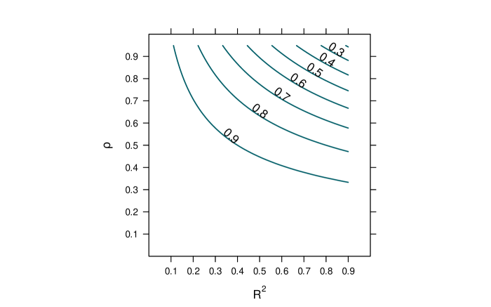
Figure 1: Theoretical fraction of residual variances shown for different values of $R^{2}=\nicefrac{{\pi^{2}}}{{\sigma^{2}}}$ and $\rho$. The numbers can be interpreted as the fraction of the sample size required in a trial adjusting for prognostic information relative to the sample size required for a trial without such an adjustment.

3.2 Sensitivity analysis

To study the impact of deviations from the distributional assumption (7), we contrasted the above presented results with a more complex DGP. For the prognostic score, we employed the process

$$s(\text{\boldmath$X$})=10\sin(\pi X_{1}X_{2})+20(X_{3}-0.5)^{2}+10X_{4}+5X_{5}+\epsilon,$$ (9)

arising from Friedman’ regression equation 1 (Friedman, 1991) with $\text{\boldmath$X$}\sim\operatorname{U}(0,1)^{10}$ and $\epsilon\sim\operatorname{N}(0,1)$. The marginal density of $s(\text{\boldmath$X$})$ is shown in Figure 2.

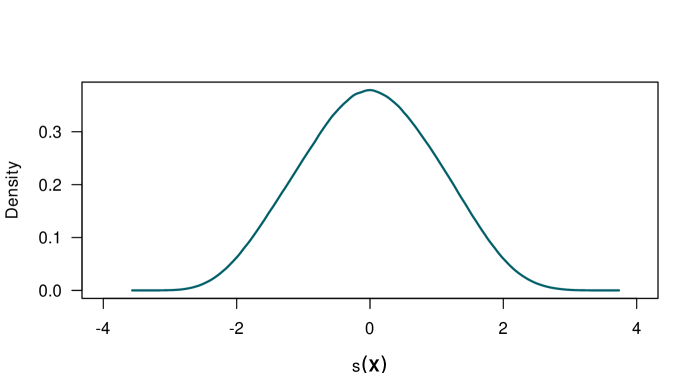
Figure 2: Prognostic score. Illustration of the density function of the prognostic score $s(\text{\boldmath$X$})$ drawn from DGP (9). The standardised prognostic score, whilst generated from a non-linear function of $X$ including interaction terms, approximately follows a standard normal distribution.

We simulated historical control data $(z=0)$ of varying sample size $\mathfrak{n}=$ 50, 100, and 10’000 as well as trial data with sample size $n=$ 1’000 from DGP (1) with $\sigma^{2}=1$ for different values of $\pi\in(0,1)$ and repeated the experiment 1’000 times. We estimated the prognostic model $\mathfrak{s}(\text{\boldmath$X$})$ from the simulated historical control data with a random forest and fitted a normal linear regression model for the treatment effect to the trial data and a model additionally adjusting for the prognostic score estimate $\mathfrak{s}(\text{\boldmath$x$})$.

Figure 3: Simulated fraction of residual variances in a model with prognostic score as defined in (9). The fractions are shown for the normal linear model regressing on the treatment effect ($\mathbb{E}(Y\mid z)$; left), and the model additionally adjusting for the prognostic score estimate ($\mathbb{E}(Y\mid z,\mathfrak{s}(\text{\boldmath$x$}))$; right) for various values of $R^{2}=\nicefrac{{\pi^{2}}}{{\sigma^{2}}}$ and different sample sizes $\mathfrak{n}=$ 50, 100, and 10’000. The green line depicts the theoretical fraction $1-R^{2}\hat{\rho}^{2}$, with the precision of the random forest $\hat{\rho}$ estimated from the data. The variance reduction predicted by the “design factor” (Borm et al., 2007) is shown as blue dashed line.

The results in Figure 3 convey similar findings as obtained theoretically. The residual variance when adjusting for the prognostic score estimated from historical data decreases with higher $R^{2}$, which translates into higher precision of the treatment effect estimates $\hat{\beta}$ (Figure 4).

Figure 4: Simulated distribution of the treatment effect estimate. The treatment effect estimates $\hat{\beta}$ from the normal linear model regressing on the treatment effect ($\mathbb{E}(Y\mid z)$; left), and the model additionally adjusting for the prognostic score estimate ($\mathbb{E}(Y\mid z,\mathfrak{s}(\text{\boldmath$x$}))$; right) are shown for various values of $R^{2}=\nicefrac{{\pi^{2}}}{{\sigma^{2}}}$ and different sample sizes $\mathfrak{n}=$ 50, 100, and 10’000. The true treatment effect $\beta=0.12$ is indicated by the horizontal line.

3.3 Comparison of predicted and empirical variance reduction

We further compared the variance reduction achieved by prognostic score adjustment as predicted by the “design factor” $1-\widehat{R^{2}}_{\text{OOS}}$ (Borm et al., 2007), using the estimated $\widehat{R^{2}}_{\text{OOS}}$ from the prognostic random forest model on historical data, to the empirical variance reduction $1-\rho^{2}R^{2}$ in our setup. For the data generating process in Section 3.2, random forests’ $\widehat{R^{2}}_{\text{OOS}}$ was estimated using a large evaluation data set (out-of-sample). The true $R^{2}$ was calculated using $\pi^{2}/\sigma^{2}$.

The lines in Figure 3 contrast the variance reduction predicted by the “design factor” $1-\widehat{R^{2}}_{\text{OOS}}$ (Borm et al., 2007) and $1-\rho^{2}R^{2}$ (Fraction 8) with the variance reduction achieved empirically (boxplots). The latter variance reduction fits the empirical results very closely, whereas the “design factor” is biased and underestimates the actual observed variance reduction.

3.4 Illustration

A recent study by Goemans et al. (2020) reported on the development of such a prognostic score for timed 4-stair climb in Duchenne muscular dystrophy patients and discussed its potential benefits in terms of design and analysis of future trials. The explained variability ($R^{2}_{\text{OOS}}$) in the prognostic model was described to be maximally $36\%$, which according to the “design factor” would allow for a variance reduction to $64\%$ of the unadjusted analysis when employing prognostic score adjustment. Our derivation, however, indicate that this factor might underestimate the empirical reduction, which, in practice, is difficult to quantify, because $R^{2}$ and $\rho$ are unknown.

4 Discussion

In our work we studied the question, in what situations leveraging prognostic information actually pays off in practice. We presented a simple and general setup in Section 2, allowing us to assess the theoretical properties of this adjustment method without making strong distributional assumptions or limiting it to specific estimators.

In Section 3.1 we quantified the maximally attainable benefit when adjusting for a prognostic score analytically, and contrasted our findings with a more complex set-up in Section 3.2. The results suggest that leveraging prognostic baseline covariates reduces residual variability, however the magnitude of this reduction might often be irrelevant in practice. These situations can be characterised by small historical samples sizes (and as a result smaller $\rho$) and/or small $R^{2}$ of the prognostic model on historical data.

As a rough rule of thumb, sample size reductions of more than $20\%$ are achievable with an $R^{2}>.3$ on historical controls when there is a high confidence in the prognostic score, with $\rho>.8$ say, requiring a large number of historical controls and the absence of drift in $s(\text{\boldmath$X$})$. When there is more uncertainty regarding the prognostic score, with $\rho\approx.6$ for example, an $R^{2}>.5$ is necessary to obtain a $20\%$ reduction in total sample size. Likewise, the corresponding increase in precision of the treatment effect estimate can be considered for fixed samples sizes. It depends on the context whether or not such an increase is relevant: It might be a game-changer in one setup but only marginally interesting in other situations.

While it is easy to estimate $R^{2}_{\text{OOS}}$ for historical controls, estimating our model parameters $R^{2}$ and $\rho$ is less straightforward. One possibility would be to perform an interim analysis regressing the outcome $Y$ on the prognostic score $\mathfrak{s}(\text{\boldmath$X$})$ on the trial controls $(Y,\text{\boldmath$X$},z=0)$ which, after appropriate standardisation such that $\mathbb{V}(\mathfrak{s}(\text{\boldmath$X$}))=1$, gives an estimate $\widehat{\pi\rho}$ for $\pi\rho$, which, together with an estimate of the residual variance $\sigma^{2}$, can be plugged into (8). In the absence of information about $\rho$, our interpretation of the theoretical results presented here is that trial designers should definitively look into the possibility of adjusting for an established prognostic score when its $R^{2}_{\text{OOS}}$ has been demonstrated to exceed $.5$.

These findings are in agreement with earlier results quantifying the impact of covariate adjustment on the necessary sample size in clinical trials. Adjusting for a single numeric covariate $X_{1}$ is a special case of our model with $\pi s(\text{\boldmath$X$})=\pi X_{1}$ and $\rho\equiv 1$, resulting in a “design factor” of $1-R^{2}$, meaning a sample size reduction to $(1-R^{2})\times 100\%$ of original sample size is possible (Borm et al., 2007; Pocock et al., 2002; Cox and McCullagh, 1982). This “design factor” however disregards that the covariate (or equivalentely the prognostic score) might be measured with error $\rho$ or that there might be potential distribution drift.

Although accounting for prognostic information through adjustment for $\mathfrak{s}(\text{\boldmath$X$})$ seems rather unorthodox, a simpler version known as post-stratification is well established. For two strata, the prognostic score $\mathfrak{s}(\text{\boldmath$X$})\in\{0,1\}$ is an indicator for the patient’s stratum, $\rho$ an unknown prognostic parameter, typically estimated from trial data. The rational is the same: Leveraging information from historical controls (used to define reasonable strata) for reducing the residual variance while safeguarding against distribution shift or incorrectly specified strata. If available, such information further can be employed to randomise patients into more homogeneous subgroups.

In the ANCOVA framework, an interesting practical question is when it will be more beneficial to directly adjust for prognostic variables instead of adjusting for a prognostic score, or even not to adjust at all (Lesaffre and Senn, 2003). We shall discuss this issue in more details.

Suppose we have $n$ subjects in total and $k\geq 2$ prognostic covariates. (The lower bound is set at $2$ since the case $k=1$ is without interest.) The loss due to non-orthogonality, which we refer to as the imbalance effect is a random variable depending on the observed imbalance in the trial. However, choosing whether to fit the score or the covariates based on an inspection of the data has the danger of increasing the type 1 error rate. Thus there is merit in making a pre-specified choice of model which, in any case, is in line with ICHe9 recommendations. It can be shown, however, that the expected imbalance effect due to fitting $k$ covariates compared to $1$ is $(n-4)/(n-3-k)$. On the other hand the expected inflation in the mean square error (MSE), which we refer to as the mean square error effect, due to fitting a score based on historical data rather than the $k$ covariates on which it is based is $\sigma_{1}^{2}/\sigma_{k}^{2}\geq 1$, where the numerator is the expected MSE for the prognostic score and the denominator the corresponding MSE with all covariates fitted. Thus, by comparing the mean square error effect to the expected imbalance effect one can make a decision. Note that a third factor is that the residual degrees of freedom for error will lead to the $t$-table having to be entered at a less favourable point, the more covariates are fitted. As is discussed in an Appendix this further effect, which we refer to as second order precision, will favour the prognostic score.

In summary, when the trial sample size $n$ is large and only a few prognostic variables are studied, using ANCOVA without any involvement of historical data should be preferred (Borm et al., 2007; Pocock et al., 2002; Cox and McCullagh, 1982). In situations where either the trial sample size $n$ is relatively small, many and potentially unstructured prognostic variables shall be adjusted for, and a large set of $\mathfrak{n}$ historical patient records is available, it seems preferable to adjust for the prognostic score in situations where $R^{2}>.3$, because only one additional parameter needs to be estimated in a classical statistical model.

An extension to non-normal models is not straightforward. From a computational point of view, the estimation of prognostic scores on appropriate scales (log-odds or log-hazard ratios, for example), is possible by application of some machine learning procedures, e.g.,  in model-based boosting (Ridgeway, 1999; Bühlmann and Hothorn, 2007; Schmid et al., 2011). Adjusting for such prognostic scores in logistic, proportional odds, or proportional hazards regression models will lead to increasing power for testing the null hypothesis $\beta=0$ at the price of changing the interpretation of the treatment effect estimate $\hat{\beta}$ from a marginal to a conditional one (Robinson and Jewell, 1991; Ford et al., 1995; Ford and Norrie, 2002; Hernández et al., 2004; Daniel et al., 2021), owing to the fact that, unlike in non-linear models, $\pi s(\text{\boldmath$X$})$ can be absorbed into the error term (2) in the linear model (1).

Appendix A Adjusting for covariates: Gains and losses

An easy way to see the effect of fitting covariates on the efficiency of an estimator is to consider adding a binary covariate (we shall take sex as an example) to the analysis of a design that is currently balanced by treatment with $2N$ patients per arm, there being two arms in total. If the covariate is not fitted, the variance of the treatment contrast will be

$$\left(\frac{1}{2N}+\frac{1}{2N}\right)\sigma_{0}^{2}=\frac{\sigma_{0}^{2}}{N},$$

where $\sigma_{0}^{2}$ is the within-treatment groups variance, which will be estimated using $2N-2$ degrees of freedom and where the subscript 0 is used to represent that no covariates have been fitted. Now suppose that the two sexes are equally well represented but having randomised and having decoded the data, we see that the disposition of subjects by group and sex is

	Control	Treatment
Females	$f$	$2N-f$	$2N$
Males	$2N-f$	$f$	$2N$
	$2N$	$2N$	$4N=n$

where the entries in the cells represents frequencies of patients of the four types. The within-sex stratum estimates now have variances proportional to

$$\left(\frac{1}{f}+\frac{1}{2N-f}\right)\sigma_{1}^{2},$$

where the subscript 1 is used to represent that one covariate has been fitted. Note, that one degree of freedom is lost if the fitting process uses sex as a main effect in an analysis of covariance. However, strict stratification estimates the variance within strata and loses one further degree of freedom. Here we consider the former case, where the degrees of freedom available to estimate this variance are now $2N-3$. Clearly, the two within-stratum estimates are equally efficient and should be weighted equally, that is to say by one half. Thus the combined estimate will have a variance equal to

$$\left(\frac{1}{2^{2}}\frac{1}{2^{2}}\right)\left(\frac{1}{f}+\frac{1}{2N-f}\right)\sigma_{1}^{2} = \frac{1}{2}\left(\frac{2N}{f(2N-f)}\right)\sigma_{1}^{2}$$

$$= \frac{N}{f(2N-f)}\sigma_{1}^{2}.$$

Note that the divisor of this expression can be expressed as $N^{2}-(f-N)^{2}$ and that $-(f-N)^{2}\leq 0$, so that the divisor reaches its maximum when $f=N$ that is to say the design is balanced, at which point the variance will be $\sigma_{1}^{2}/N$.

We thus see that we can expect three consequences of fitting sex in the model. 1) If sex is predictive we may expect $\sigma_{1}^{2}<\sigma_{0}^{2}$. We can refer to this as the mean square error effect. 2) The variance multiplier will be

$$\frac{N}{f(2N-f)}\geq\frac{1}{N}$$

with equality only being achieved in the case of perfect balance. More generally, we may expect some imbalance and so some loss in efficiency. We can refer to this as the imbalance effect. 3) A completely predictable loss is that the degrees of freedom associated with the relevant $t$-distribution will be reduced by 1. This, unlike the other two effects, is not an effect on precision itself but an effect on our estimates of precision and may be referred to as the second order precision effect. One way of judging it is to compare the variances of the two $t$-distributions involved, using the fact that in general this is $\nu/(\nu-2)$ where $\nu$ is the degrees of freedom. In the case with no predictors, we have $\nu=n-2$ and more generally, if we have $k$ predictors, we have $\nu=n-2-k$ so that the general variance term is

$$\frac{n-2-k}{n-4-k},$$

with this reducing to $(n-2)/(n-4)$ if $k=0$, $(n-3)/(n-5)$ if $k=1$.

More generally, for the cases where covariates may be continuous and there may be more than one covariate but only two treatments, we may consider the influence of these three factors in terms of the general variance estimator $(\text{\boldmath$X$}^{\top}\text{\boldmath$X$})^{-1}\sigma_{k}^{2}$. Here $\text{\boldmath$X$}_{n\times(k+2)}$ is the design matrix for which we may assume, without loss of generality, that the first column is an intercept carrier, the second is a treatment indicator and the $k$ further columns, $k=0,1,2,\dots$ are for the covariates.

This formulation includes not fitting covariates as a special case, for which $k=0$. Note, however, that for the practical purpose of comparing using a single score based on covariates to using the original covariates themselves then the lowest value that is of any interest is $k=2$.

The diagonal elements of the $(\text{\boldmath$X$}^{\top}\text{\boldmath$X$})^{-1}$ matrix give the variance multipliers and, given what we have said about the order of the columns, the second of these is the multiplier for the variance of the treatment effect. We refer to this as $q_{k}$, where the subscript $k$ refers to the number of covariates being fitted and not to the position in the matrix . Thus the variance of the treatment estimate is $q_{k}\sigma_{k}^{2}$. Given $n$ patients it can be shown that we must have $q_{k}\geq 4/n$. For our previous example, we had $n=4N$ so we had $q_{k}\geq 1/N$.

As covariates are added to the model and therefore columns are added to the design matrix, the value of $q_{k}$ cannot reduce but may increase. The example with sex as a binary covariate illustrates this. In a randomised design the effect on $q$ is not predictable as the design matrix will vary randomly but for normally distributed predictors the expected effect may be described. If the trial is balanced in the sense that there are the same number of patients on each of the two arms but otherwise randomised, the expected value is given by

$$\mathbb{E}(q_{k})=\frac{4}{n}\frac{n-3}{n-3-k}.$$

Special cases are

$$\mathbb{E}(q_{0})=\frac{4}{n}\frac{n-3}{n-3}=\frac{4}{n},$$

$$\mathbb{E}(q_{1})=\frac{4}{n}\frac{n-3}{n-4}.$$

It thus follows that we have

$$\frac{\mathbb{E}(q_{k})}{\mathbb{E}(q_{0})}=\frac{n-3}{n-3-k},$$

$$\frac{\mathbb{E}(q_{k})}{\mathbb{E}(q_{1})}=\frac{n-4}{n-3-k},$$

the second of these being relevant to the task of comparing adjustment for a single score based on $k$ covariates to independently fitting them all them all. Note that this formula does not depend on the covariates being generated by an independent process. (The covariates, could, for example, be correlated.) This is because, given $k$ predictors and assuming that the set has no redundancy (the generating process is of rank $k$), they can be replaced by $k$ orthogonal predictors which together will have the same identical predictive value as the original $k$. Furthermore, if we have a predictive score, which is a linear combination of the predictors, then given $k-1$ predictors and the score, the value of the remaining predictor is completely determined and so redundant. Thus the formula for $\mathbb{E}(q_{k})/\mathbb{E}(q_{1})$ is valid for this case also.

Thus, consider making a decision as to whether to fit such a score. A relevant comparison is that of the ratio of the two expected mean square errors to the ratio of the expected imbalance factors. Thus a sufficient condition for fitting such a score would be

$$\frac{\sigma_{1}^{2}}{\sigma_{k}^{2}}\leq\frac{n-4}{n-3-k},\ 2\leq k\leq n-4$$

where $\sigma_{1}^{2}$ is the mean square error fitting the score as a single covariate. Note that the right-hand side of the expression is an expectation but a known quantity that must be greater than one (in expectation). The left-hand side is a random variable, which also ought to be greater than one, and some judgement must be made by the modeller as to what it will be. The lower bound of $k$ is the lowest value of interest and the higher bound is the highest for which the expression on the right-hand side is defined.

One could also try to incorporate the second order second order precision effect into the decision process. Note, however, that this is always in favour of using the score rather than the $k$ individual predictors. Therefore, if the condition above is satisfied it will definitely be an advantage to fit the score. This is why we refer to the condition as sufficient.

However, it should be noted, that the expression provides a means of guiding the choice between fitting $k$ predictors and fitting a linear combination of them all. If $k\geq 3$ it is possible that fitting a reduced set would be better than either.

References

- Aikens et al. (2020) Aikens RC, Greaves D, Baiocchi M (2020). “A Pilot Design for Observational Studies: Using Abundant Data Thoughtfully.” Statistics in Medicine, 39(30), 4821–4840. 10.1002/sim.8754.
- Arbogast and Ray (2009) Arbogast PG, Ray WA (2009). “Use of Disease Risk Scores in Pharmacoepidemiologic Studies.” Statistical Methods in Medical Research, 18(1), 67–80. 10.1177/0962280208092347.
- Arbogast and Ray (2011) Arbogast PG, Ray WA (2011). “Performance of Disease Risk Scores, Propensity Scores, and Traditional Multivariable Outcome Regression in the Presence of Multiple Confounders.” American Journal of Epidemiology, 174(5), 613–620. 10.1093/aje/kwr143.
- Borm et al. (2007) Borm GF, Fransen J, Lemmens WA (2007). “A Simple Sample Size Formula for Analysis of Covariance in Randomized Clinical Trials.” Journal of Clinical Epidemiology, 60(12), 1234–1238. 10.1016/j.jclinepi.2007.02.006.
- Branders et al. (2021) Branders S, Pereira A, Bernard G, Ernst M, Albert A (2021). “Leveraging Historical Data for High-Dimensional Regression Adjustment, a Composite Covariate Approach.” arXiv: 2103.14421.
- Bühlmann and Hothorn (2007) Bühlmann P, Hothorn T (2007). “Boosting Algorithms: Regularization, Prediction and Model Fitting.” Statistical Science, 22(4), 477–505. 10.1214/07-sts242.
- Cellini et al. (2019) Cellini F, Manfrida S, Deodato F, Cilla S, Maranzano E, Pergolizzi S, Arcidiacono F, Di Franco R, Pastore F, Muto M, et al. (2019). “Pain REduction with Bone Metastases STereotactic Radiotherapy (PREST): A Phase III Randomized Multicentric Trial.” Trials, 20(1), 1–7. 10.1186/s13063-019-3676-x.
- Cox and McCullagh (1982) Cox DR, McCullagh P (1982). “A Biometrics Invited Paper with Discussion. Some Aspects of Analysis of Covariance.” Biometrics, 38(3), 541–561. 10.2307/2530040.
- Daniel et al. (2021) Daniel R, Zhang J, Farewell D (2021). “Making Apples from Oranges: Comparing Noncollapsible Effect Estimators and Their Standard Errors after Adjustment for Different Covariate Sets.” Biometrical Journal, 63(3), 528–557. 10.1002/bimj.201900297.
- Ford and Norrie (2002) Ford I, Norrie J (2002). “The Role of Covariates in Estimating Treatment Effects and Risk in Long-term Clinical Trials.” Statistics in Medicine, 21(19), 2899–2908. 10.1002/sim.1294.
- Ford et al. (1995) Ford I, Norrie J, Ahmadi S (1995). “Model Inconsistency, Illustrated by the Cox Proportional Hazards Model.” Statistics in Medicine, 14(8), 735–746. 10.1002/sim.4780140804.
- Friedman (1991) Friedman JH (1991). “Multivariate Adaptive Regression Splines.” The Annals of Statistics, 19(1), 1–67. 10.1214/aos/1176347963.
- Goemans et al. (2020) Goemans N, Wong B, Van den Hauwe M, Signorovitch J, Sajeev G, Cox D, Landry J, Jenkins M, Dieye I, Yao Z, Hossain I, Ward SJ, the Collaborative Trajectory Analysis Project (cTAP) (2020). “Prognostic Factors for Changes in the Timed 4-Stair Climb in Patients with Duchenne Muscular Dystrophy, and Implications for Measuring Drug Efficacy: A Multi-Institutional Collaboration.” PLOS One, 15(6). 10.1371/journal.pone.0232870.
- Hansen (2008) Hansen BB (2008). “The Prognostic Analogue of the Propensity Score.” Biometrika, 95(2), 481–488. 10.1093/biomet/asn004.
- Hernández et al. (2004) Hernández AV, Steyerberg EW, Habbema JDF (2004). “Covariate Adjustment in Randomized Controlled Trials with Dichotomous Outcomes Increases Statistical Power and Reduces Sample Size Requirements.” Journal of Clinical Epidemiology, 57(5), 454–460. 10.1016/j.jclinepi.2003.09.014.
- Herrera et al. (2020) Herrera AF, Li H, Castellino SM, Rutherford SC, Davison K, Evans AG, Punnett A, Constine LS, Hodgson DC, Parsons SK, Prica A, Kostakoglu L, Shipp MA, Laubach C, Leblanc ML, Crump M, Kahl BS, Leonard JP, Kelly KM, Smith SM, Friedberg JW (2020). “SWOG S1826: A Phase III, Randomized Study of Nivolumab Plus AVD or Brentuximab Vedotin Plus AVD in Patients with Newly Diagnosed Advanced Stage Classical Hodgkin Lymphoma.” Blood, 136(Supplement 1), 23–24. 10.1182/blood-2020-136422.
- Hurwitz et al. (2018) Hurwitz H, Van Cutsem E, Bendell J, Hidalgo M, Li CP, Salvo MG, Macarulla T, Sahai V, Sama A, Greeno E, Yu KH, Verslype C, Dawkins F, Walker C, Clark J, O’Reilly EM (2018). “Ruxolitinib+ capecitabine in advanced/metastatic pancreatic cancer after disease progression/intolerance to first-line therapy: JANUS 1 and 2 randomized phase III studies.” Investigational New Drugs, 36(4), 683–695. 10.1007/s10637-018-0580-2.
- Kernan et al. (1999) Kernan WN, Viscoli CM, Makuch RW, Brass LM, Horwitz RI (1999). “Stratified Randomization for Clinical Trials.” Journal of Clinical Epidemiology, 52(1), 19–26. 10.1016/s0895-4356(98)00138-3.
- Knaus et al. (1991) Knaus WA, Wagner DP, Draper EA, Zimmerman JE, Bergner M, Bastos PG, Sirio CA, Murphy DJ, Lotring T, Damiano A, Harrell FE (1991). “The APACHE III Prognostic System: Risk Prediction of Hospital Mortality for Critically III Hospitalized Adults.” Chest, 100(6), 1619–1636. 10.1378/chest.100.6.1619.
- Kopp-Schneider et al. (2020) Kopp-Schneider A, Calderazzo S, Wiesenfarth M (2020). “Power Gains by Using External Information in Clinical Trials Are Typically Not Possible When Requiring Strict Type I Error Control.” Biometrical Journal, 62(2), 361–374. 10.1002/bimj.201800395.
- Kreuz et al. (2020) Kreuz M, Otto DJ, Fuessel S, Blumert C, Bertram C, Bartsch S, Loeffler D, Puppel SH, Rade M, Buschmann T, Christ S, Erdmann K, Friedrich M, Froehner M, Muders MH, Schreiber S, Specht M, Toma MI, Benigni F, Freschi M, Gandaglia G, Briganti A, Baretton GB, Loeffler M, Hackermüller J, Reiche K, Wirth M, Horn F (2020). “ProstaTrend – A Multivariable Prognostic RNA Expression Score for Aggressive Prostate Cancer.” European Urology, 78(3), 452–459. 10.1016/j.eururo.2020.06.001.
- Lesaffre and Senn (2003) Lesaffre E, Senn S (2003). “A Note on Non-parametric ANCOVA for Covariate Adjustment in Randomized Clinical Trials.” Statistics in Medicine, 22(23), 3583–3596. 10.1002/sim.1583.
- Nguyen et al. (2020) Nguyen TL, Collins GS, Pellegrini F, Moons KGM, Debray TPA (2020). “On the Aggregation of Published Prognostic Scores for Causal Inference in Observational Studies.” Statistics in Medicine, 39(10), 1440–1457. 10.1002/sim.8489.
- Pocock et al. (2002) Pocock SJ, Assmann SE, Enos LE, Kasten LE (2002). “Subgroup Analysis, Covariate Adjustment and Baseline Comparisons in Clinical Trial Reporting: Current Practice and Problems.” Statistics in Medicine, 21(19), 2917–2930. 10.1002/sim.1296.
- Ridgeway (1999) Ridgeway G (1999). “The State of Boosting.” Computing Science and Statistics, 31, 172–181.
- Robinson and Jewell (1991) Robinson LD, Jewell NP (1991). “Some Surprising Results about Covariate Adjustment in Logistic Regression Models.” International Statistical Review / Revue Internationale De Statistique, 59(2), 227–240. 10.2307/1403444.
- Saffi et al. (2014) Saffi MAL, Polanczyk CA, Rabelo-Silva ER (2014). “Lifestyle Interventions Reduce Cardiovascular Risk in Patients with Coronary Artery Disease: A Randomized Clinical Trial.” European Journal of Cardiovascular Nursing, 13(5), 436–443. 10.1177/1474515113505396.
- Schmid et al. (2011) Schmid M, Hothorn T, Maloney KO, Weller DE, Potapov S (2011). “Geoadditive Regression Modeling of Stream Biological Condition.” Environmental and Ecological Statistics, 18(4), 709–733. 10.1007/s10651-010-0158-4.
- Schuler et al. (2021) Schuler A, Walsh D, Hall D, Walsh J, Fisher C (2021). “Increasing the Efficiency of Randomized Trial Estimates via Linear Adjustment for a Prognostic Score.” arXiv: 2012.09935.
- Steingrimsson et al. (2017) Steingrimsson JA, Hanley DF, Rosenblum M (2017). “Improving Precision by Adjusting for Prognostic Baseline Variables in Randomized Trials with Binary Outcomes, without Regression Model Assumptions.” Contemporary Clinical Trials, 54, 18–24. 10.1016/j.cct.2016.12.026.
- Wijdicks et al. (2005) Wijdicks EFM, Bamlet WR, Maramattom BV, Manno EM, McClelland RL (2005). “Validation of a New Coma Scale: The FOUR Score.” Annals of Neurology, 58(4), 585–593. 10.1002/ana.20611.
- Wyss et al. (2016) Wyss R, Glynn RJ, Gagne JJ (2016). “A Review of Disease Risk Scores and their Application in Pharmacoepidemiology.” Current Epidemiology Reports, 3(4), 277–284. 10.1007/s40471-016-0088-2.
- Zhang and Ma (2019) Zhang Z, Ma S (2019). “Machine Learning Methods for Leveraging Baseline Covariate Information to Improve the Efficiency of Clinical Trials.” Statistics in Medicine, 38(10), 1703–1714. 10.1002/sim.8054.