Abstract

Objectives

We generate via advanced Deep Learning (DL) techniques artificial leaf images in an automatized way. Our aim is to dispose of a source of training samples in artificial intelligence applications for modern crop management in agriculture, with focus on disease recognition on plant leaves. Such applications require large amounts of data and, while leaf images are not truly scarce, image collection and annotation remains a very time–consuming process. Data scarcity can be addressed by augmentation techniques consisting in simple transformations of samples belonging to a small dataset, but the richness of the augmented data is limited: this motivates the search for alternative approaches.

Methods

Pursuing an approach based on DL generative models, we propose a Leaf-to-Leaf Translation (L2L) procedure structured in two steps: firstly, a residual variational autoencoder architecture is used to generate synthetic leaf skeletons (leaf profile and veins) starting from companions binarized skeletons of real leaf images. In a second step, we perform the process of translation via a Pix2pix framework, which uses conditional generator adversarial networks to reproduce the colorization of leaf blades, preserving the shape and the venation pattern.

Results

The L2L procedure generates synthetic images of leaves with a realistic appearance. We address the performance measurement both in a qualitative and a quantitative way; for this latter evaluation, we employ a DL anomaly detection strategy which quantifies the degree of anomaly of synthetic leaves with respect to real samples.

Conclusions

Generative DL approaches have the potential to be a new paradigm to provide low-cost meaningful synthetic samples for computer-aided applications. The present L2L approach represents a step towards this goal, being able to generate synthetic samples with a relevant qualitative and quantitative resemblance to real leaves.

Author summary

In this work we present an end-to-end workflow incorporating state-of-the-art Deep Learning strategies based on generative methods to produce realistic synthetic images of leaves. At the best of our knowledge, this is the first attempt of such an approach to this problem. Our focus application is the training of neural networks for modern crop management systems in agriculture, but we believe that many other computer–aided applications may benefit from it. We take inspiration from previous works carried out on eye retina image synthesis, an application domain which shares some similarities with the present problem (a venation pattern over a colorized “fundus”). Our approach relies on the successive use of autoencoders and generative adversarial architectures, able to generate leaf images both in the Red-Green-Blue channels as well as in the Near-Infra-Red. The generated leaf images have a realistic appearance even if they sometimes suffer from small inconsistencies, especially discolored patches. A quantitative evaluation via an anomaly detection algorithm shows that in average a synthetic sample is classified as such only in 25% of the cases.

Introduction

The ability to generate meaningful synthetic images of leaves is highly desirable for many computer-aided applications. At the best of our knowledge, attempts at generating synthetic images of leaves have been made mostly in the field of computer graphics and were aimed at creating the illusion of realistic landscapes covered with plants, trees or meadows. These efforts were mainly based on procedural mathematical models describing the venation structure and the color/texture of the leaf. A specific type of formal grammar, called L–grammar, was developed to generate instructions to draw a leaf. Several instances of the profile of leaves of a certain species were created upon random variations of parameters of the directives of a certain L–grammar [1]. Biologically-motivated models were also proposed. A main point of these approaches is the representation of the interaction between auxin sources distributed over the leaf blade and the formation of vein patterns [2]. Some attempts were also carried out using finite elements to build mechanistic models of the leaf blade, tuned on its structural parameters [3]. After generating the leaf shape and venation pattern - regardless of the approach- texture and colors were rendered by a color palette prescribed by the user or generated according to a pseudo–random algorithm. A color model based on convolution sums of divisor functions was proposed in [4], while a shading model based on the PROSPECT model for light transmission in leaves [5], was proposed in [6]. “Virtual rice” leaves were created in [7] based on a RGB-SPAD model.

In this work we aim at introducing a radically different approach by generating artificial images of leaves by automatized techniques based on Deep Learning (DL) techniques. Our focus is mainly to enrich dataset of leaf images for neural networks training, even if we deem that the present approach may be of interest also in a wide range of other fields, starting from computer graphics. The motivation underlying this work is that DL methods require a large amount of data – often of the order of hundreds of thousands of images – to avoid overfitting phenomena. Data augmentation is a common remedy, usually consisting in simple transformations such as random rotations, translations or deformations of the original images. However, the richness of the augmented dataset is limited and more sophisticated approaches for synthesizing additional training data have a greater potential to improve the training process. In this respect, DL generative models represent attractive methods to produce synthetic images (with corresponding labels) using the information from a limited set of real, unlabeled images of the same domain. This idea is not new - in absolute - but it has been used mainly in the field of medicine, where data may be extremely scarce and difficult to obtain (see, e.g., the recent review [8]). In the present context, while scarcity of leaf images may be not a real issue, what is more relevant is to avoid the huge mole of work required to collect, examine and annotate images. This is especially true when image segmentation should be performed, which is a pixel-wise problem: the acquisition of annotated segmentation masks is exceedingly costly and time consuming, as a human expert annotator has to label every pixel manually. For our model we take inspiration from [9] (and reference therein), where the authors synthesised eye retina images. The fundus of the eye shares indeed several characteristics with our problem: a fine network of hierarchically organized blood vessels (leaf veins) superposed to a colored background (leaf blade). In addition, in our problem the leaf blade is also characterized by a specific silhouette that must be represented as well. We propose a Leaf-to-Leaf Translation (L2L) approach to obtain synthetic colorized leaf blades organized in two steps: first we use a residual variational autoencoder architecture to generate fake leaf skeletons starting from binarized companion skeletons of real leaf images. In a second step we perform the process of translation via a Pix2pix framework, which uses conditional generator adversarial networks (cGANs) to reproduce the specific color distribution of the leaf blade, preserving leaf shape and venation pattern. We carry out both qualitative and quantitative evaluations of the degree of realism of the synthetic samples of leaves. Specifically, a DL-based anomaly detection strategy is used to evaluate the distance (“anomaly”) between synthetic and real samples. The results show a good degree of realism, that is a low anomaly score, and indicate that with the present approach one can significantly enrich a small dataset and improve the training performance of DL architectures.

Materials and methods

Dataset

Grapevine leaves were imaged via a QSi640 ws-Multispectral camera (Atik Cameras, UK) equipped with a Kodak 4.2 Mp micro-lens image sensor and 8 spectral selection filters operating in the bands 430 to 740 nm. For the purpose of this experiment, leaves were imaged singularly on a dark background, under controlled diffuse illumination conditions. Images were acquired in the single spectral channels 430 nm (blue, B), 530 nm (green, G), 685 nm (red, R) and 740 nm (near–infrared, NIR). These channels are typically considered when dealing with the task of recognition of plant diseases in a multispectral analysis approach [10, 11]. A set of RGB images of the same leaves in standard CIE color space were also acquired for reference. Camera parameters were set and image collection was performed via an in–house developed acquisition software written in MATLAB. Reflectance calibration was carried out by including in each image 3 reflectance references (Spectralon R = 0.02, R = 0.50 and R = 0.99; Labsphere, USA). We obtained photos of 80 leaves with a resolution of $2048\times 2048$ pixels and 8 bit for each channel. Preprocessing operations were performed on each image: removal of hot pixels, normalization along each channel according to the reference probes, creation of a companion binarized skeleton image. For this latter procedure, the NIR channel was used, since it presents an a high contrast between the leaf and background. The skeleton comprises the profile of the leaf and the vein pattern. Images and companion skeletons were resized at $256\times 256$ resolution. Fig 1 shows the original images in the RGB and RGNIR spaces, the normalized NIR channel and the corresponding companion skeleton. Before using the generative algorithms, we performed standard data augmentation by randomly flipping each image horizontally and vertically, rotating by an angle randomly chosen in $[-\pi/4,\pi/4]$ and finally zooming with a random amount in the range $[-20\%,+20\%]$. The dataset was thus increased in this way from 80 to 240 samples.

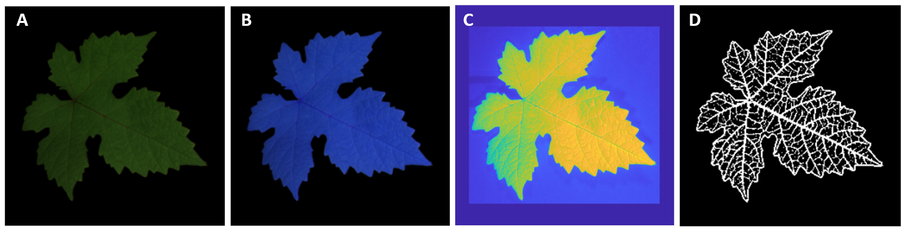
Fig 1: Sample of grapevine leaf from the dataset. A: RGB image; B: RGNIR image; C: normalized and cropped NIR image; D: companion skeleton. In the skeleton binarized image, the white color identifies the leaf profile and veins, the black color identifies other parts of the leaf and the background.

Generative methods for L2L translation

The authors of [9, 12] generated artificial patterns of blood vessels along with corresponding eye fundus images using a common strategy which divides the problem of the image generation into two sub–problems, each one addressed by a tailored DL architecture: first they generate the blood vessel tree, then they color the eye fundus. We adopt this very approach, first generating the leaf profile and veins and then coloring the leaf blade. Also in our experience this approach has turned out to be more effective than generating the synthetic image altogether.

Skeleton Generation

According to the above considerations, the generation of a realistic leaf skeleton is the first step towards the final goal of our work. For this task, we use a convolutory autoencoder architecture, that is, a network trained to reconstruct its input. An autoencoder (AE) is composed of two submodels: 1) an encoder $Q$ that maps the training dataset to a latent (hidden) representation $z$; 2) a decoder $P$ that maps $z$ to an output that aims to be a plausible replica of the input. We have experimented that simple autoencoders cannot generate realistic skeletons. For this reason, we use a more sophisticated architecture, called Residual Variational Autoencoder (ResVAE, see Fig 2).

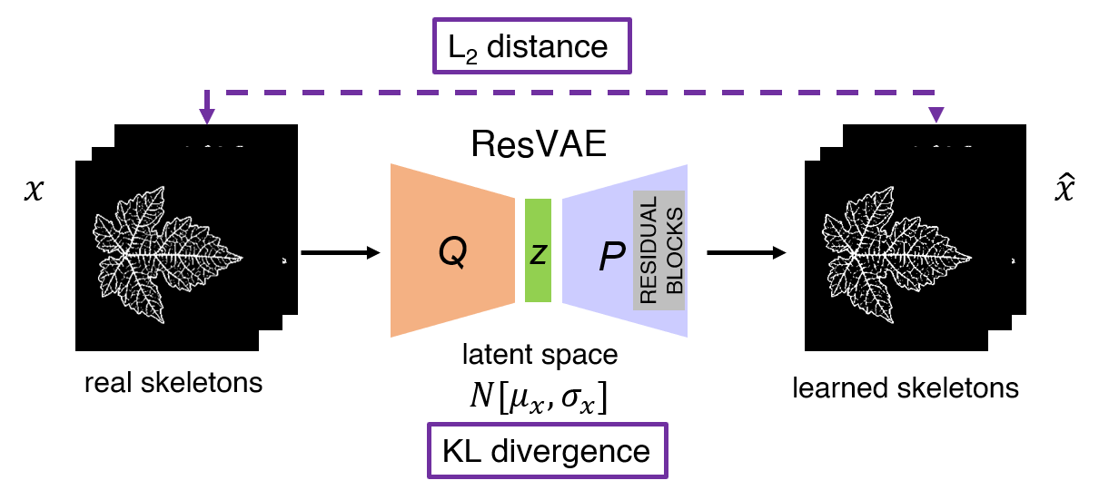
Fig 2: Illustration of the ResVAE framework (training).

This learning framework has already been successfully applied to image recognition, object detection, and image super-resolution (see, e.g., [13]). In the data generation framework, AEs learn the projection of the initial data into a latent subspace, and then a sample of this subspace is randomly extracted to build up a new instance of the initial data. Instead of learning such projection, VAEs learn the probability distribution of the latent variables given the input $x$. As a matter of fact, a variational autoencoder can be defined as an autoencoder whose training is regularized to avoid overfitting and ensure that the latent space has good properties that enable the generative process. To achieve this goal, instead of encoding an input as a single point, VAEs encode it as a (Gaussian) distribution over the latent space, where $p(z|x)$ represents the probability of the latent variable $z$ given the input $x$. The decoding part consists in sampling a variable from $p(z|x)$ and then providing a reconstruction $\widehat{x}$ of the initial data $x$. We associate to this framework the following loss function

$$\mathcal{L}_{\text{VAE}}(x,\hat{x})=\mathcal{L}_{L_{2}}(x,\hat{x})+\beta\mathcal{L}_{KL}\left(p(z|x),\mathcal{N}(0,1)\right),$$ (1)

where the first term $\mathcal{L}_{L_{2}}=||x-\widehat{x}||^{2}$ is the $L_{2}$ norm of the reconstruction loss, and the second term $\mathcal{L}_{KL}=KL[N(\mu_{x},\sigma_{x}),N(0,1)]$ is the Kullback–Leibler (KL) divergence [14, 15] The KL divergence enhances sparsity in neurons activation to improve the quality of the latent features keeping the corresponding distribution close to the Gaussian distribution $\mathcal{N}(0,1)$. The tunable regularization hyperparameter $\beta$ is used to weigh the two contributions[16]. With respect to VAEs, ResVAEs additionally employ residual blocks and connection skips. The idea beyond residual blocks is the following [17]: normal layers try to directly learn an underlying mapping, say $h(x)$, while residual ones approximate a residual function $r(x)=h(x)-x$. Once the learning is complete, $r(x)$ is added to the input to retrieve the mapping: $h(x)=r(x)+x$. In our architecture, residual blocks are concatenated to the decoder to increase the capacity of model [13]. The connection skips allow to back–propagate the gradients more efficiently giving the bottleneck more access to the simpler features extracted earlier in the encoder. The resulting ResVAE compresses $256\times 256$ leaf skeleton images to a low dimension latent vector of size 32 and then it reconstructs it to $256\times 256$ images. We refer to S1 Appendix for specifications of the present ResVAE architecture.

Translation to colorized leaf image

We consider the colorization of the leaf out of an existing skeleton as an image-to- image translation problem, which implies to learn a mapping from the binary vessel map into another representation. Similarly to what observed in [9] for retinal image generation, many leaf images can share a similar binary skeleton network due to variations in color, texture, illumination. For this reason, learning the mapping is an ill-posed problem and some uncertainty is present. We learn the mapping via a Pix2pix net (also known as conditional GAN, (cGAN)), an unsupervised generative model which represents a variation of a standard GAN. As such it includes two deep neural networks, a generator $G$ and discriminator $D$. The generator aims to capture the data distribution, while the discriminator estimates the probability that a sample actually came from the training data rather than from the generator. In order to learn a generative distribution over the data $x$, the generator builds a mapping $G(z;\theta_{G})$ from a prior noise distribution $p_{z}$ to the image data space, $\theta_{G}$ being the generator parameters. The discriminator outputs the probability that $x$ came from the real data distribution $p_{data}(x)$ rather from the generated one. We denote by $D(x;\theta_{D})$ the discriminator function, $\theta_{D}$ being the discriminator parameters. In standard GANs, the optimal mappings $G^{*}$ is obtained as the equilibrium point of the min–max game:

$$(G^{*},D^{*})=\arg\displaystyle\min_{G}\max_{D}\mathcal{L}_{GAN}(D,G),$$

where we have defined the objective function

$$\mathcal{L}_{GAN}(D,G):=\mathbb{E}_{x\sim p_{data}(x)}[\log D(x;\theta_{D})]+\mathbb{E}_{z\sim p_{z}(z)}[\log(1-D(G(z;\theta_{G})))].$$ (2)

In the conditional framework, an extra variable $y$ is added as a further source of information on $G$, which combines the noise prior $p_{z}(z)$ and $y$. The objective function thus becomes

$$\mathcal{L}_{cGAN}(D,G)=\mathbb{E}_{x\sim p_{data}(x)}[\log D(x;\theta_{D})]+\mathbb{E}_{z\sim p_{z}(z)}[\log(1-D(G(z|y;\theta_{G})))].$$ (3)

Previous approaches have found it beneficial to mix the GAN objective with a more traditional loss, such as $L_{2}$ distance [18]. The discriminator’s job remains unchanged, but the generator is bound not only to fool the discriminator but also to stay near the ground truth output in an $L_{2}$ sense. In this work we rather explore the use of the $L_{1}$ distance rather than $L_{2}$ as $L_{1}$ promotes sparsity and at the same time it encourages less blurring [19]:

$$\mathcal{L}_{L_{1}}(G)=\mathbb{E}_{x,y,z}[||y-G(z|y;\theta_{G})||].$$ (4)

The final objective is thus

$$(G^{*},D^{*})=\arg\min_{G}\max_{D}\mathcal{L}_{cGAN}(D,G)+\lambda\mathcal{L}_{L_{1}}(G)$$ (5)

where $\lambda$ is a regularization hyperparameter. In our implementation the extra information corresponds to the leaf skeletons which condition $G$ in the image generation task to preserve leaf shape and venation pattern. The discriminator is provided with skeleton plus generated image pairs and must determine whether the generated image is a plausible (feature preserving) translation. Fig 3 shows the training process of the cGAN. We refer to S2 Appendix for specifications of the Pix2pix architecture we adopted.

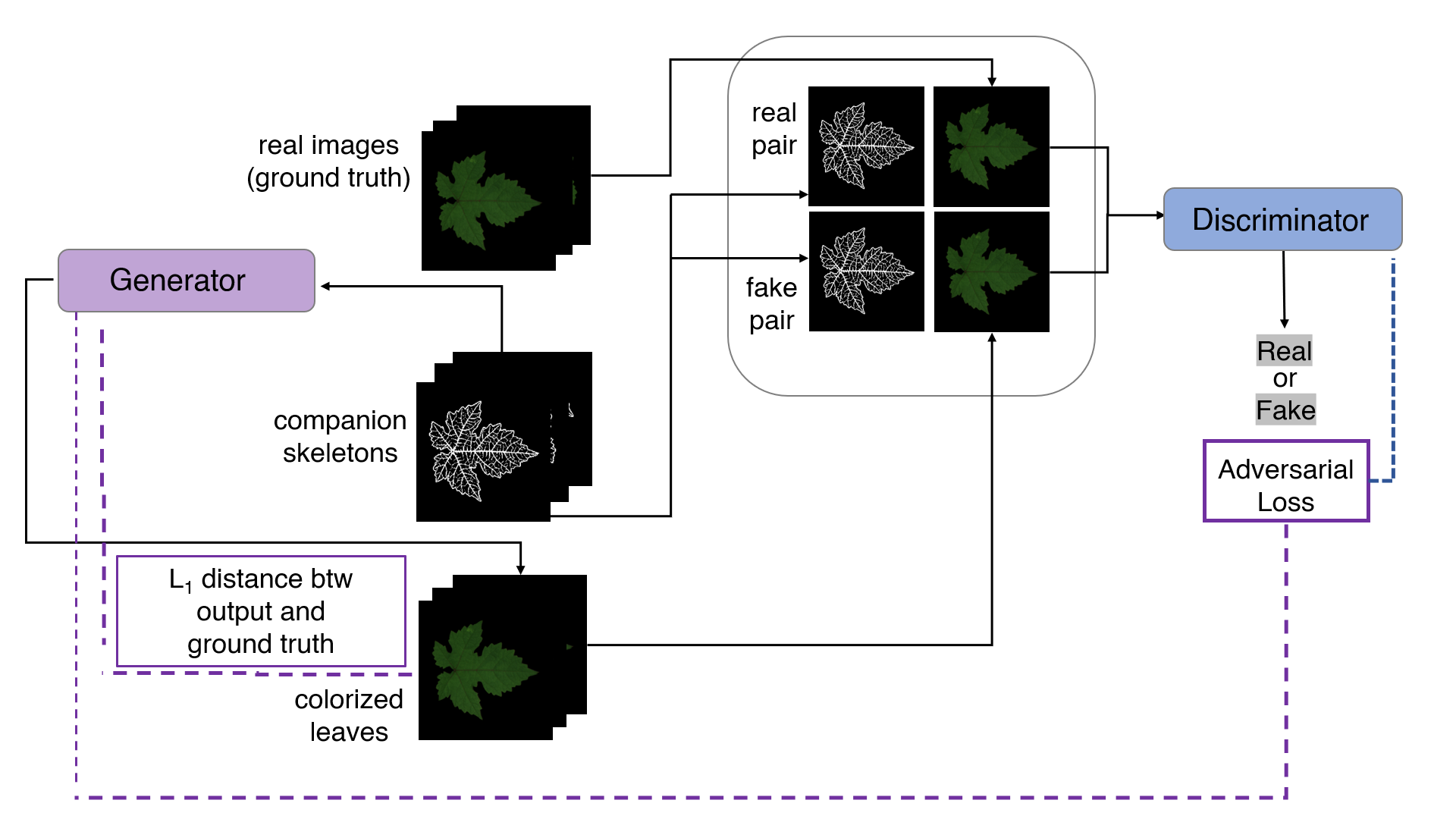
Fig 3: Illustration of the Pix2Pix framework (training).

L2L workflow: from random samples to leaf images

Upon training of the ResVAE and Pix2pix architectures, we dispose of an end-to-end procedure for the generation of synthetic leaves. The procedure, which is completely unsupervised, can be summarized as follows (see also Fig 4):

1. Load weights of the trained ResVAE decoder and Pix2pix generator.

2. Draw a random vector from a normal distribution whose parameters are chosen according to the ResVAE latent space representation (note that its size equals the dimension of the latent space used in the ResVAE, 32 in the present case).

3. Input the random vector in the trained ResVAE decoder and generate a leaf skeleton

4. Input the leaf skeleton into the trained generator of the Pix2Pix net to translate it into a fully colorized leaf.

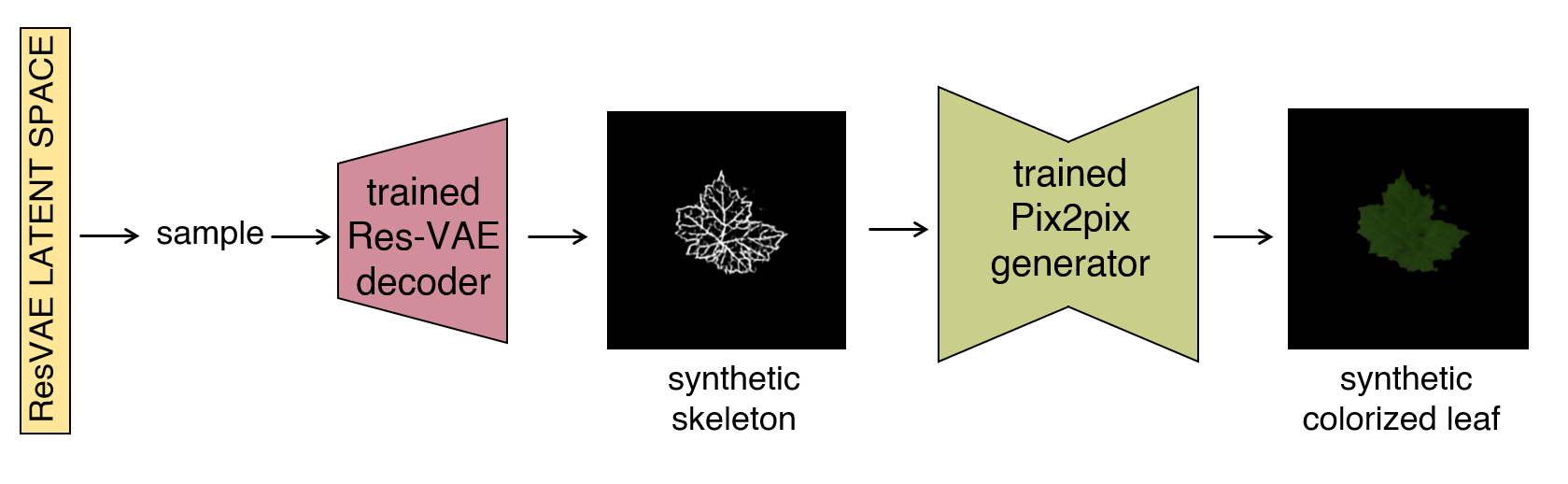
Fig 4: L2L workflow illustration. A random input vector is drawn from the ResVAE latent space representation and is input into the trained ResVAE decoder. This latter outputs a synthetic leaf skeleton, which in turn is fed into the trained generator of the Pix2Pix and translated into a corresponding colorized leaf.

Results and Discussion

The proposed technique can be employed to generate as many synthetic leaf images as the user requires. The model has been implemented with Keras . Upon generation of the synthetic images, their quality is assessed performing both experimental qualitative (visual) and quantitative evaluations as follows.

Visual qualitative evaluation

Consistency test. Beforehand, we have evaluated the consistency of the methodology by verifying that the net has learned to translate a leaf sample comprised in the training set into itself. Fig 5 shows an example of this test. The generated leaf is very similar to the real one, except for some vein discoloration and a small blurring effect effect, which is a well–known product of AEs employed in image generation [20].

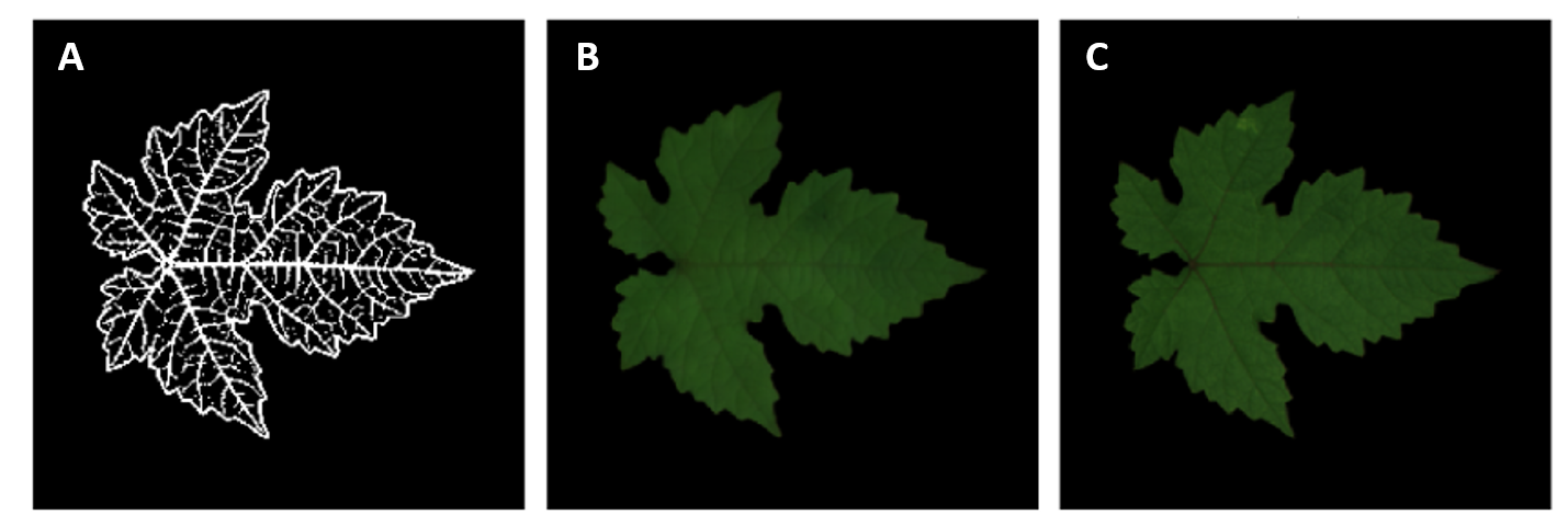
Fig 5: Consistency test. The companion binarized leaf skeleton of a real leaf is passed through the generator of the Pix2Pix net to check whether the synthetic colorized leaf blade is similar to the original one. A: companion skeleton of a real leaf; B: synthetic colorized blade generated; C: original leaf.

Translation from unseen real companion skeleton. Having ensured that the model has learned to translate on the training data, we verify that it is able to produce reliable synthetic images using skeletons obtained from leaves that are not part of the training dataset. Fig 6 shows an instance of colorized leaf obtained from this test.

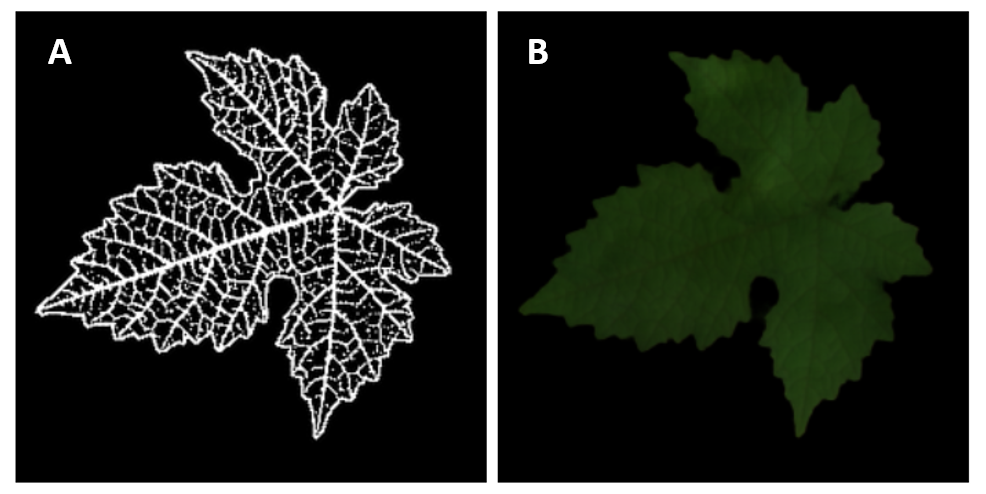
Fig 6: Translation from unseen real companion skeleton. A binarized leaf skeleton companion of a real leaf not belonging to the training set is passed through the generator of the Pix2Pix net to check. A: companion skeleton; B: synthetic colorized blade.

Full L2L translation Fig 7 shows several instances of synthetic colorized leaves obtained starting from different random latent vectors. Note that the generated leaf images differ in terms of their global appearance, that is the model generalizes and does not trivially memorizes the examples. As a note, one should observe that some discolored parts may be appear. Moreover, sometimes the skeletons show small artifacts consisting in not–connected pixels positioned outside the leaf boundary (not appearing in Fig 7). This latter issue will be addressed via a refinement algorithm explained below.

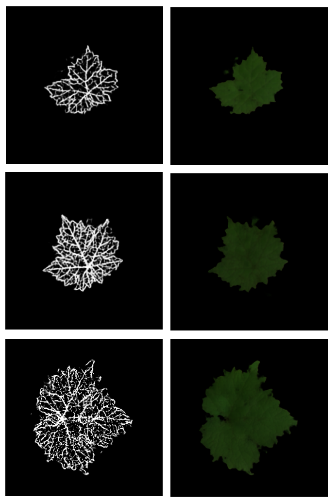
Fig 7: Full L2L translation results. Examples of synthetic colorized leaves along with the corresponding synthetic companion skeletons.

L2L-RGNIR translation As mentioned above, applications in crop management require to have at disposal images also in the NIR channel. To do this, we use the L2L generation procedure as for the RGB channels starting from RGNIR images as Pix2Pix targets. Since the same leaf skeletons are used, it is not necessary to re-train the ResVAE if this procedure has been already carried out for the RGB case. Fig 8 shows some results of this model.

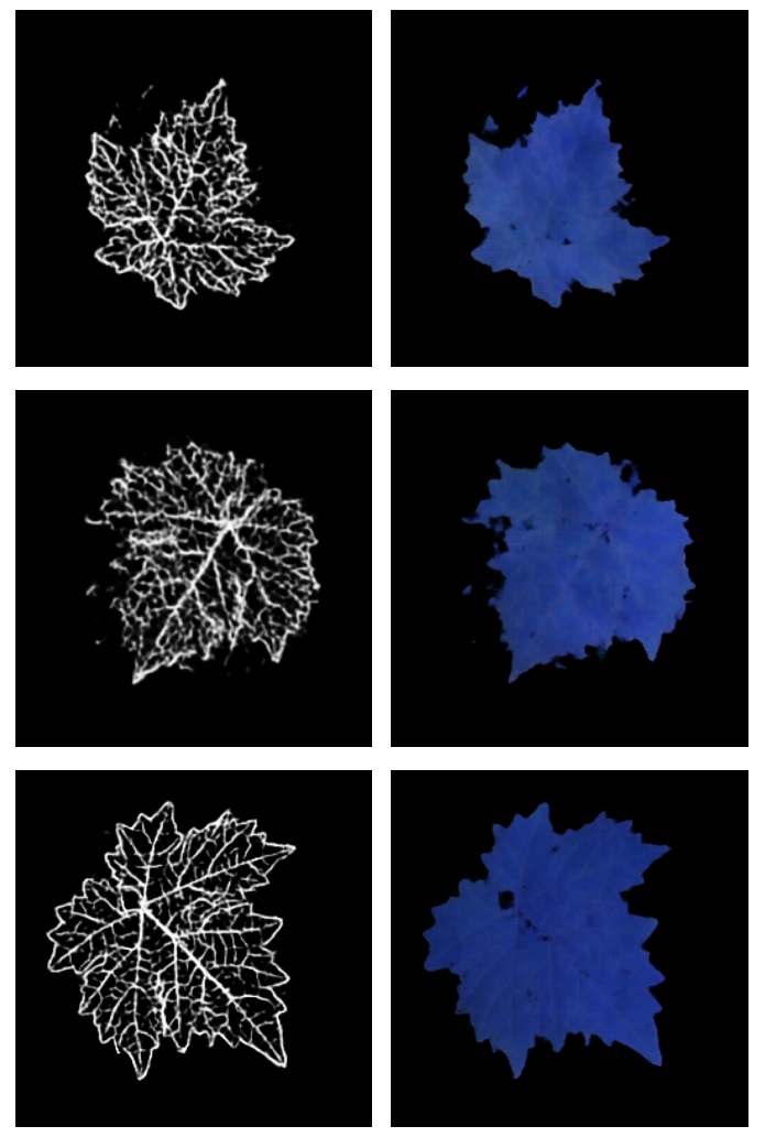
Fig 8: L2L-RGNIR translation results. Examples of synthetic leaves colorized in the RGNIR channels along with the corresponding synthetic companion skeletons.

Refinement algorithm. We have already discussed the fact that synthetically generated images may sometimes present artifacts (leaf regions that appear detached from the leaf blade). Obviously this is not realistic and we need to remove such artifacts. The refinement algorithm is implemented at present in a procedural way and it is based on the idea of finding the contours of all the objects and removing all objects laying outside the leaf contour. Note that this procedure must pay attention to leave internal holes intact, because in nature such holes are the result of the superposition of leaf lobes or due to several abiotic/biotic conditions. Fig 9 shows the first leaf in Fig 7 which presents artifacts (panel A, zoomed area including the artifact in panel B) and its cleaned counterpart (panel C).

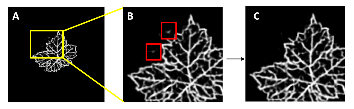
Fig 9: Refinement algorithm. The generative procedure sometimes produces artifacts, that is leaf regions that appear outside the leaf blade. These artifacts are corrected by procedurally finding the contours of all the objects in the image and removing the objects outside the leaf contour. A: first leaf in Fig 7 presenting artifacts; B: inset showing the magnified artifacts; C: cleaned leaf.

Quantitative Quality Evaluation

In order to assess quantitatively the quality of the generated leaves, we employ a DL–based anomaly detection strategy. This approach is discussed in detail in [21], here we briefly recall the main points. The strategy consists in training an AE to compress real leaf images in a latent subspace and then reconstruct the images using the latent representation (see Skeleton Generation section for the same concept). Once the network is trained in this way, we feed it with a synthetic image generated by our procedure. The AE encodes it in the latent space and tries to recover the original image according to its training rules. Since the net has been trained to be the identity operator for real images, if the artificial images are substantially different, an anomalous reconstruction is obtained. Fig 10 provides a visual schematization of this approach. The figure also details the score system used to detect the anomaly.

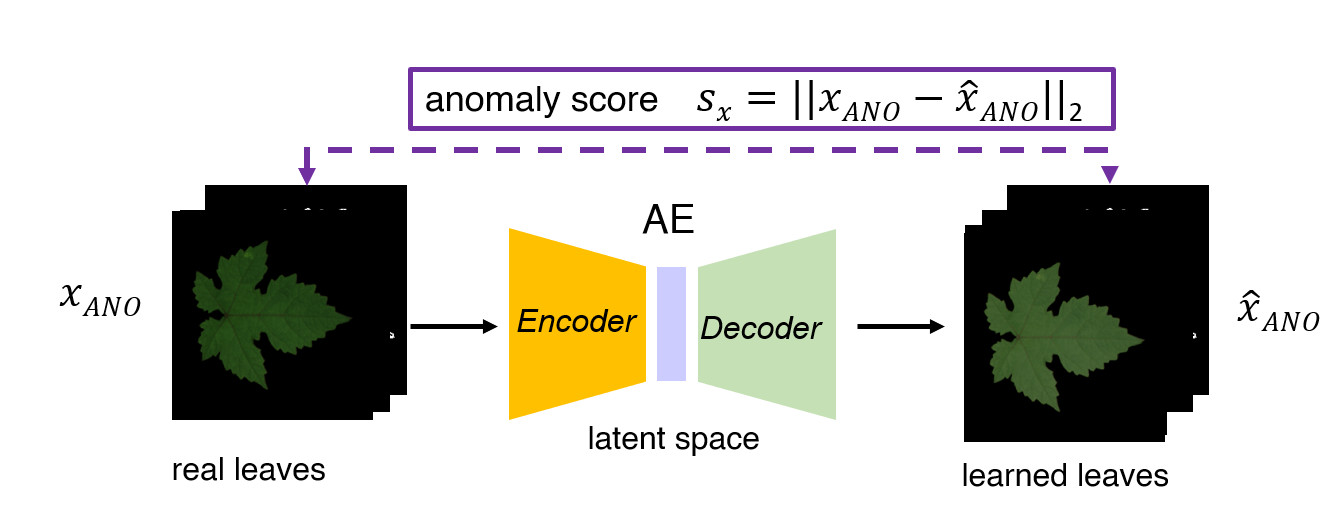
Fig 10: AE for anomaly detection. The AE is trained with images of real leaves to be the identity operator of the input. A synthetic leaf with a low level of similarity is recognized as an anomaly if fed into the trained AE and its anomaly score $s_{x}$ is high.

The degree of anomaly is quantified via the ROC curve and its area, the AUC index [22]. For this latter, we found AUC=0.25, which means that for a random synthetic image fed into the AE, there is a 25% of possibility to classify it as an anomaly, that is to be synthetic instead or real. While this result does not indicate a perfect reconstruction of the real leaves, it shows that the synthetic leaves are a reasonably accurate surrogate of real leaves and can be used for a first massive training at a very low cost. A successive refinement can then be applied using a limited number of real leaves upon transfer learning.

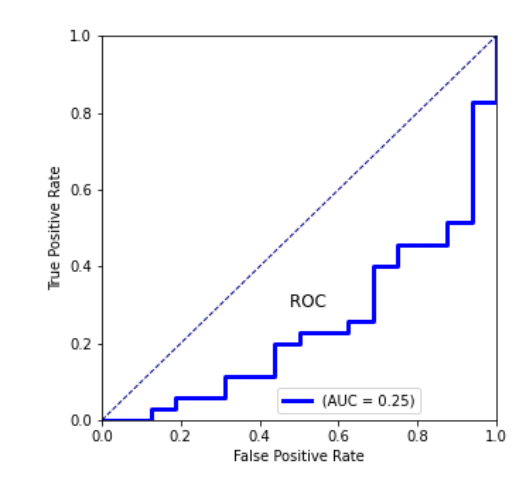
Fig 11: Quantification of anomaly via ROC curve and AUC index. A point on the ROC curve represents - for a certain threshold on the anomaly score - the false positive rate (genuinely real images) vs the true positive rate (genuinely synthetic images). The value AUC=0.25 means that a synthetic image is (mis–)classified as synthetic in the 25% of cases. The dotted line represents the result one would obtain by tossing a coin to decide whether an image is artificial or real.

Conclusion

Goal of this work was to explore advanced DL generative methods to produce realistic images of leaves to be used in computer–aided applications The main focus was on the generation of artificial samples of leaves to be used to train DL networks for modern crop management systems in precision agriculture. Disposing of synthetic samples which have a reasonable resemblance to real samples alleviates the burden of manually collecting and annotating hundreds of data. The Pix2pix net performs good translations from the leaf skeletons generated by the ResVAE, except for some discolored parts, both for the colorization of RGB and RGNIR images. Also, the leaves generated by ResVAE have sometimes pixels positioned outside the boundary which, if not corrected, can cause artifacts in the synthetic leaves. An easy procedure has been proposed as well to correct these artifacts. We believe that the generative approach can significantly contribute to automatize the process of building a low-cost training set for DL applications. Several computer–aided applications may also benefit of such a strategy, where many samples are required, possibly with different degree of accuracy in the representation.

Author contribution

Conceptualization: Alessandro Benfenati, Paola Causin
Dataset: Alessandro Benfenati, Davide Bolzi, Paola Causin, Roberto Oberti
Methodology: Alessandro Benfenati, Davide Bolzi, Paola Causin
Implementation: Davide Bolzi
Analysis: Alessandro Benfenati, Davide Bolzi, Paola Causin, Roberto Oberti
Writing: Alessandro Benfenati, Paola Causin

Supporting information

S1 Appendix

Implementation and training of the ResVAE neural network. The architecture, inspired by the one described in [23], is shown in Fig 12.

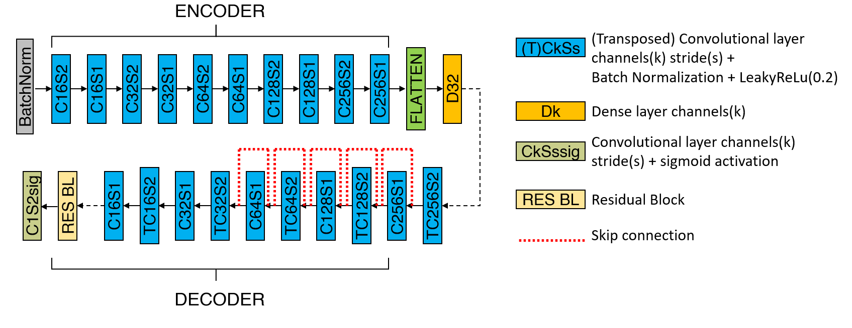
Fig 12: ResVAE architecture. Building blocks of the encoder and decoder components of the ResVAE. The convolutional filters have kernels of size $4\times 4$. The Residual block is formed by 5 convolutional layers of 16 filters each with kernel of size $4\times 4$ and stride equal to 1, followed by a Batch Normalization layer and LeakyReLU activation function.

The training is performed via a stochastic gradient descent strategy, with gradients computed by standard back–propagation; we use the Adam optimizer with learning rate $\eta=0.001$ and we train the model for 2000 epochs with a batch size of 64. After a hyper–parameter search, $\beta$ in the loss function (1) was set to 75.

S2 Appendix

Implementation and training of the Pix2pix neural network.

The Pix2pix is a GAN architecture designed for image-to-image translation, originally presented in [19] and comprising a generator and a discriminator. The discriminator is deep neural network that performs image classification. It takes both the source image (leaf skeleton) and the target image (colorized leaf) as input and predicts the likelihood of whether the target image is real or a fake translation of the source image. We use a PatchGAN model which tries to establish whether each $N\times N$ (local) patch in the image is real or fake. We run this discriminator convolutionally across the image, averaging all responses to provide the ultimate output of the discriminator. The generator is an encoder-decoder model using a U-Net architecture with feature-map concatenation between two corresponding blocks of the encoder/decoder. The encoder and decoder of the generator are comprised of standardized blocks of convolution, batch normalization, dropout, and activation layers. We proceed as suggested in [19]: the generator is updated via a weighted sum of both the adversarial loss and the $L_{1}$ loss, where the parameter $\lambda$ in the loss function eq5 is set to 100 in order to encourage the generator to produce plausible translations of the input image, and not just plausible images in the target domain. We initialize the generator/discriminator weights with a normal distribution of zero mean and standard deviation $\sigma=0.002$; we use the Adam optimizer with a learning rate $\eta=0.0002$ and we train the generator/discriminator paired model for 12000 training steps, using a batch size of 1. Fig 13 shows the generator and discriminator architectures.

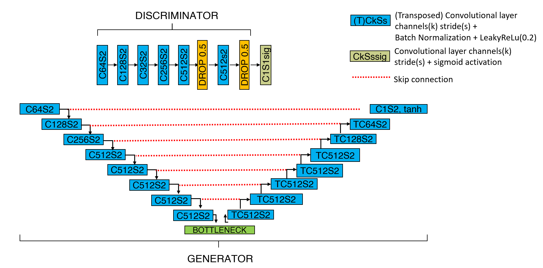
Fig 13: Pix2pix architecture. Building blocks of the generator and discriminator components.

References

- 1. Peyrat A, Terraz O, Merillou S, Galin E. Generating vast varieties of realistic leaves with parametric 2Gmap L-systems. Vis Comput. 2008;24(7):807–816.
- 2. Runions A, Fuhrer M, Lane B, Federl P, Rolland-Lagan AG, Prusinkiewicz P. Modeling and visualization of leaf venation patterns. In: ACM SIGGRAPH 2005 Papers; 2005. p. 702–711.
- 3. Samee SB. Modeling and Simulation of Tree Leaves Using Image-Based Finite Element Analysis. PhD Thesis, University of Cincinnati; 2012.
- 4. Kim D, Kim J. Procedural modeling and visualization of multiple leaves. Multimed Sys. 2017;23(4):435–449.
- 5. Féret JB, Gitelson A, Noble S, Jacquemoud S. PROSPECT-D: towards modeling leaf optical properties through a complete lifecycle. Remote Sens Environ. 2017;193:204–215.
- 6. Miao T, Zhao C, Guo X, Lu S. A framework for plant leaf modeling and shading. Math Comput Model. 2013;58(3-4):710–718.
- 7. Yi Wl, He Hj, Wang Lp, Yang Hy. Modeling and simulation of leaf color based on virtual rice. DEStech Trans Mater Sci Eng. 2016;(mmme).
- 8. Taghanaki SA, Abhishek K, Cohen JP, Cohen-Adad J, Hamarneh G. Deep semantic segmentation of natural and medical images: a review. Artif Intell Rev. 2021;54(1):137–178.
- 9. Costa P, Galdran A, Meyer MI, Niemeijer M, Abràmoff M, Mendonça AM, et al. End-to-end adversarial retinal image synthesis. IEEE Trans Med Imaging. 2017;37(3):781–791.
- 10. Oberti R, Marchi M, Tirelli P, Calcante A, Iriti M, Borghese AN. Automatic detection of powdery mildew on grapevine leaves by image analysis: Optimal view-angle range to increase the sensitivity. Comput Electron Agric. 2014;104:1–8.
- 11. Mahlein AK, Kuska MT, Behmann J, Polder G, Walter A. Hyperspectral sensors and imaging technologies in phytopathology: state of the art. Annu Rev Phytopathol. 2018;56:535–558.
- 12. Sengupta S, Athwale A, Gulati T, Zelek J, Lakshminarayanan V. FunSyn-Net: enhanced residual variational auto-encoder and image-to-image translation network for fundus image synthesis. In: Medical Imaging 2020: Image Processing. vol. 11313. International Society for Optics and Photonics; 2020. p. 113132M.
- 13. Cai L, Gao H, Ji S. Multi-stage variational auto-encoders for coarse-to-fine image generation. In: Proceedings of the 2019 SIAM International Conference on Data Mining. SIAM; 2019. p. 630–638.
- 14. Asperti A, Trentin M. Balancing Reconstruction Error and Kullback-Leibler Divergence in Variational Autoencoders. IEEE Access. 2020;8:199440–199448.
- 15. Benfenati A, Ruggiero V. Image regularization for Poisson data. Journal of Physics: Conference Series. 2015 nov;657:012011. Available from: https://doi.org/10.1088/1742-6596/657/1/012011.
- 16. Higgins I, Matthey L, Pal A, Burgess C, Glorot X, Botvinick M, et al. -VAE: Learning basic visual concepts with a constrained variational framework. In: ICLR 2017 Conference Proceedings; 2017. .
- 17. He K, Zhang X, Ren S, Sun J. Deep residual learning for image recognition. In: Proceedings of the IEEE conference on computer vision and pattern recognition; 2016. p. 770–778.
- 18. Kurach K, Lučić M, Zhai X, Michalski M, Gelly S. A large-scale study on regularization and normalization in GANs. In: International Conference on Machine Learning. PMLR; 2019. p. 3581–3590.
- 19. Isola P, Zhu JY, Zhou T, Efros AA. Image-to-image translation with conditional adversarial networks. In: Proceedings of the IEEE conference on computer vision and pattern recognition; 2017. p. 1125–1134.
- 20. Huang H, Li Z, He R, Sun Z, Tan T. Introvae: Introspective variational autoencoders for photographic image synthesis. arXiv preprint arXiv:180706358. 2018;.
- 21. Benfenati A, Causin P, Oberti R, Stefanello G. Unsupervised feature–oriented deep learning techniques for powdery mildew recognition based on multispectral imaging. submitted;.
- 22. Bradley AP. The use of the area under the ROC curve in the evaluation of machine learning algorithms. Pattern Recognit. 1997;30(7):1145–1159.
- 23. Chollet F. Variational AutoEncoder; 2020. https://keras.io/examples/generative/vae/.