Integral State-Feedback Control of Linear Time-Varying Systems: A Performance Preserving Approach

Abstract

An integral extension of state-feedback controllers for linear time-varying plants is proposed, which preserves performance of the nominal controller in the unperturbed case. Similar to time-invariant state feedback with integral action, the controller achieves complete rejection of disturbances whose effective action on the plant is constant with respect to the control input. Moreover, bounded-input bounded-state stability with respect to arbitrary disturbances is shown. A modification for preventing controller windup as well as tuning guidelines are discussed. The efficacy of the proposed technique is demonstrated in simulation for a two-tank system that is linearized along a time-varying reference trajectory.

,

1 Introduction

The design of controllers containing open-loop integrators is one of the main tools for reducing the impact of slowly varying disturbances. When considering set-point regulation of time-invariant plants, for example, such controllers can completely reject the influence of small parameter deviations and constant disturbances in steady state. Techniques for designing such controllers have therefore seen extensive research, and some of the basic techniques are nowadays part of a typical curriculum on control systems, see e.g. Franklin et al. (1986).

As an alternative to integral control, disturbance observer based control has seen extensive research, see, for example, the recent reviews by Bakhshande and Söffker (2015); Chen et al. (2016); Sariyildiz et al. (2020) and references therein. In this framework, the disturbance is estimated by an observer and then cancelled by the control law. The connection to integral control is the well-known internal model principle: with integral controllers, the integral part implicitly reconstructs the disturbance, while disturbance observers contain an explicit disturbance model.

In the time-varying case, rejection of disturbances by means of integral control or disturbance observers is more challenging. For example, even constant disturbances can only be reconstructed if their time-varying influence on the plant is accurately known. Moreover, their cancellation typically requires the disturbances to be matched, i.e., to act in the same channel as the control inputs. In practice, time-varying dynamics often occur when linearizing nonlinear plants along time-varying references, cf. e.g., Shao and Wang (2014). The possible performance improvement in this case, also in presence of more general (e.g., slowly varying) disturbances makes the use of integral-type controllers desirable in practice.

The present paper proposes an extension of a given time-varying state-feedback control law by an integral part while preserving its performance in the nominal case. A similar goal may also be achieved by extending an existing observer by a disturbance estimate. Such an extension, however, may require redesign or retuning of the entire observer. Moreover, when the modeled disturbance is not matched, and hence cannot be cancelled straightforwardly, obtaining the final control law typically requires further effort. The proposed approach, in contrast, requires little additional design effort, is easy to tune by means of an integral gain satisfying only a lower (but no upper) bound, and—being a standard integral control—is straightforward to add to almost any control architecture without significant modifications.

While the design of integral controllers is very well studied in general, there are only few explicit works on the time-varying case. Most recent works consider it in the context of trajectory linearization control, see Shao and Wang (2014); Qiu et al. (2019), and apply established techniques, such as feedback linearization, cf. Palanki and Kravaris (1997), or time-varying LQR designs using an extended state space as in Athans and Falb (2013); Kalman (1960), see also e.g. Attia et al. (2020). These techniques do not allow to easily preserve the performance of a nominal controller, however. The corresponding design of disturbance observers (sometimes called PI observers in case of constant disturbances) also is considered in the time-invariant case mostly; some of the few works on the time-varying case are found in Kaczorek (1979, 1980); Shafai and Carroll (1985). That design is based on a transformation to a normal form, however, which requires differentiability of the system coefficients. More recent works, such as Ichalal and Mammar (2015); Do et al. (2020); Chen et al. (2020), handle time-varying systems in a linear parameter-varying (LPV) framework. This typically leads to conservative designs, however, as the obtained controllers typically are valid for arbitrary parameter variations within a convex set.

The approach presented in this paper is based on an idea recently proposed for the time-invariant, single-input single-output case in Seeber and Moreno (2020). Here, this idea is extended to the time-varying, multivariable case. Moreover, issues relevant in practice are addressed in the form of tuning insight and a modification to prevent integrator windup.

The paper is structured as follows: After some preliminaries in Section 2, Section 3 introduces the problem statement and discusses the class of disturbances to be rejected. The performance preserving integral state-feedback controller is then proposed in Section 4, and conditions for disturbance rejection and asymptotic stability are given. The actual stability analysis and the corresponding proofs are contained in Section 5. Section 6 discusses various issues that may be useful in a practical context: a modification to mitigate windup in the presence of limited control inputs, and an insight into the tuning of controller parameters. Two special cases, the case of output-feedback integral action and the time-invariant case, are discussed in Section 7. Section 8, finally, applies the proposed approach in simulation to a two-tank system linearized along a time-varying reference trajectory. Section 9 draws conclusions.

2 Preliminaries

This section discusses some notational conventions and stability notions that are used throughout the paper. Matrices and vectors are denoted by boldface capital and boldface lowercase letters, respectively. The largest and smallest eigenvalue of a symmetric matrix $\mathbf{M}=\mathbf{M}^{\mathrm{T}}$ are denoted by $\lambda_{\mathrm{max}}(\mathbf{M})$ and $\lambda_{\mathrm{min}}(\mathbf{M})$, respectively, the identity matrix is denoted by $\mathbf{I}$, and $\left\lVert\mathbf{v}\right\rVert$ or $\left\lVert\mathbf{M}\right\rVert$ mean the (induced) 2-norm of a vector $\mathbf{v}$ or a matrix $\mathbf{M}$.

In dynamical systems, differentiation of a vector $\mathbf{x}$ with respect to time $t$ is expressed as $\dot{\mathbf{x}}$. When writing such systems, time dependence of state (usually $\mathbf{x}$) and input (usually $\mathbf{u}$ or $\mathbf{w}$) is suppressed and only time dependence of the system’s parameters is stated explicitly. Furthermore, all time-varying system parameters are assumed to be uniformly bounded with respect to time.

Some stability notions for linear time-varying systems are discussed next. For systems without inputs, the notions of asymptotic stability and uniform exponential stability, see, e.g. Anderson et al. (2013), will be relevant.

Definition 1.

The linear system $\dot{\mathbf{x}}=\mathbf{A}(t)\mathbf{x}$ is called

1. asymptotically stable (AS), if its origin is Lyapunov stable and every solution $\mathbf{x}(t)$ satisfies $\lim_{t\to\infty}\mathbf{x}(t)=\bm{0}$;

2. uniformly exponentially stable (UES), if there exist positive constants $\mu$ and $M$ such that

   $$\left\lVert\mathbf{x}(t)\right\rVert\leq M\mathrm{e}^{-\mu(t-t_{0})}\left\lVert\mathbf{x}(t_{0})\right\rVert$$ (1)

   holds for every solution $\mathbf{x}(t)$ and every $t_{0}$.

Uniform exponential stability provides some robustness in the presence of bounded, vanishing disturbances:

Lemma 2 ((Hahn, 1967, Theorem 59.1)).

Let $\dot{\mathbf{x}}=\mathbf{A}(t)\mathbf{x}$ be uniformly exponentially stable and consider the perturbed system $\dot{\mathbf{x}}=\mathbf{A}(t)\mathbf{x}+\mathbf{w}(t)$. If the disturbance $\mathbf{w}(t)$ is uniformly bounded and satisfies $\lim_{t\to\infty}\mathbf{w}(t)=\bm{0}$, then $\lim_{t\to\infty}\mathbf{x}(t)=\bm{0}$ holds for the perturbed system.

If the initial state is set to zero, the boundedness of the system’s state in the presence of a bounded input is guaranteed by uniform bounded-input, bounded-state stability as introduced in the following.

Definition 3.

The linear system $\dot{\mathbf{x}}=\mathbf{A}(t)\mathbf{x}+\mathbf{B}(t)\mathbf{w}$ with input $\mathbf{w}$ is called uniformly bounded-input bounded-state stable with respect to $\mathbf{w}$, if there exists a finite positive constant $\gamma$ such that for any $t_{0}$ and any input signal $\mathbf{w}(t)$, the corresponding zero-state response satisfies

$$\sup_{t\geq t_{0}}\left\lVert\mathbf{x}(t)\right\rVert\leq\gamma\sup_{t\geq t_{0}}\left\lVert\mathbf{w}(\tau)\right\rVert.$$ (2)

It is well known that for a uniformly bounded matrix $\mathbf{B}(t)$, uniform exponential stability of the autonomous system guarantees uniform bounded-input bounded-state stability, see, e.g. (Rugh, 1995, Lemma 12.4).

3 Problem Statement

Consider a linear time-varying plant

$$\dot{\mathbf{x}} =\mathbf{A}(t)\mathbf{x}+\mathbf{B}(t)\mathbf{u}+\mathbf{F}(t)\mathbf{w}$$ (3a)

$$\mathbf{y} =\mathbf{C}(t)\mathbf{x}$$ (3b)

with a fully measurable state vector $\mathbf{x}\in\mathbb{R}^{n}$, a control input $\mathbf{u}\in\mathbb{R}^{l}$, an output $\mathbf{y}\in\mathbb{R}^{m}$, and an external disturbance $\mathbf{w}\in\mathbb{R}^{p}$. The matrices $\mathbf{A}(t)$, $\mathbf{B}(t),\mathbf{F}(t),\mathbf{C}(t)$ are piecewise continuous and uniformly bounded with respect to $t$.

The goal is to design a control law that asymptotically stabilizes the perturbed plant for a certain class of disturbances in the sense of the following definition:

Definition 4.

A control law is said to asymptotically stabilize the perturbed plant (3) with respect to a certain class of perturbations, if the closed loop is asymptotically stable for $\mathbf{w}=\bm{0}$ and $\lim_{t\to\infty}\mathbf{x}(t)=\bm{0}$ holds for trajectories with all perturbations from the class.

The design proposed in this paper is based on extending a given nominal (static) state-feedback controller by an integral action such that

1. the perturbed plant is asymptotically stabilized for a certain class of perturbations (specified below),

2. the plant is rendered uniformly bounded-input bounded-state stable with respect to arbitrary perturbations, and

3. the nominal performance is preserved in the sense that, in the unperturbed case, behavior is identical to that obtained with the nominal controller.

Remark 5.

Note that reference tracking for a linear plant $\dot{\mathbf{z}}=\mathbf{A}(t)\mathbf{z}+\mathbf{B}(t)\mathbf{q}+\mathbf{F}(t)\mathbf{w}$ can also be reduced to a stabilization problem as considered above. To see that, let $\mathbf{z}_{\mathrm{ref}}(t)$ and $\mathbf{q}_{\mathrm{ref}}(t)$ be a reference trajectory and input satisfying $\dot{\mathbf{z}}_{\mathrm{ref}}(t)=\mathbf{A}(t)\mathbf{z}_{\mathrm{ref}}(t)+\mathbf{B}(t)\mathbf{q}_{\mathrm{ref}}(t)$. Then, system (3a) is obtained by choosing $\mathbf{x}=\mathbf{z}-\mathbf{z}_{\mathrm{ref}}(t)$ and $\mathbf{q}=\mathbf{u}+\mathbf{q}_{\mathrm{ref}}(t)$. Alternatively, if the reference input $\mathbf{q}_{\mathrm{ref}}$ is unknown, one can also use $\mathbf{q}=\mathbf{u}$ and augment the disturbance vector $\mathbf{w}$ by $\mathbf{q}_{\mathrm{ref}}$.

In the following, the assumptions regarding the nominal controller and the considered class of disturbances are discussed.

3.1 Nominal State-Feedback Controller

As a starting point for the considered controller design, a (static) time-varying state-feedback controller of the form

$$\mathbf{u}=-\mathbf{K}(t)\mathbf{x}$$ (4)

with a uniformly bounded $\mathbf{K}(t)\in\mathbb{R}^{l\times n}$ is assumed to be given. It is assumed that the given state feedback renders the unperturbed plant, i.e., (3a) with $\mathbf{w}=\bm{0}$, uniformly exponentially stable. This leads to the following formal assumption regarding the nominal closed loop.

Assumption 6.

The state-feedback gain $\mathbf{K}(t)$ is such that the unperturbed, nominal closed-loop system

$$\dot{\mathbf{x}}=\bigl{[}\mathbf{A}(t)-\mathbf{B}(t)\mathbf{K}(t)\bigr{]}\mathbf{x}$$ (5)

is uniformly exponentially stable.

Remark 7.

Such a nominal controller may, for example, be designed by solving a Riccati differential equation, see e.g. Kalman (1960), or by means of spectrum assignment techniques, see e.g. Zhu (1997); Babiarz et al. (2021).

3.2 Disturbance Class for Asymptotic Stabilization

In the time-invariant case, it is well-known that controllers with integral action can only compensate for (asymptotically) constant disturbances. In the time-varying case, not the disturbance itself, but its action with respect to the control input needs to be constant. This leads to the following specification of disturbances, for which asymptotic stabilization of the plant can reasonably be expected.

Definition 8.

A bounded disturbance $\mathbf{w}(t)$ is called asymptotically constant with respect to the control input, if there exists a constant vector $\overline{\mathbf{w}}_{0}$ such that

$$\lim_{t\to\infty}\bigl{[}\mathbf{F}(t)\mathbf{w}(t)-\mathbf{B}(t)\overline{\mathbf{w}}_{0}\bigr{]}=\bm{0}$$ (6)

holds.

An important special case occurs when the disturbance is matched or asymptotically matched in the sense of the following definitions:

Definition 9.

The disturbance in (3) is called matched or asymptotically matched, respectively, if there exists a piecewise continuous and uniformly bounded matching matrix $\mathbf{D}(t)$ such that $\mathbf{F}(t)-\mathbf{B}(t)\mathbf{D}(t)=\bm{0}$ holds either for all $t$ or as $t\to\infty$.

Clearly, a matched disturbance is also asymptotically matched. In these cases, the considered class of disturbances may be specified in a simpler way using the following proposition:

Proposition 10.

Consider system (3) and suppose that the disturbance is bounded and asymptotically matched with matching matrix $\mathbf{D}(t)$. Then, $\mathbf{w}(t)$ is asymptotically constant with respect to the control input if $\lim_{t\to\infty}\mathbf{D}(t)\mathbf{w}(t)$ exists.

Proof 3.1.

Set $\overline{\mathbf{w}}_{0}=\lim_{t\to\infty}\mathbf{D}(t)\mathbf{w}(t)$ and note that

$$\mathbf{F}(t)\mathbf{w}(t)-\mathbf{B}(t)\overline{\mathbf{w}}_{0} =\bigl{(}\mathbf{F}(t)-\mathbf{B}(t)\mathbf{D}(t)\bigr{)}\mathbf{w}(t)$$

$$\quad+\mathbf{B}(t)\bigl{(}\mathbf{D}(t)\mathbf{w}(t)-\overline{\mathbf{w}}_{0}\bigr{)}.$$ (7)

Since $\mathbf{F}(t)-\mathbf{B}(t)\mathbf{D}(t)$ and $\mathbf{D}(t)\mathbf{w}(t)-\overline{\mathbf{w}}_{0}$ tend to zero while $\mathbf{w}(t)$ and $\mathbf{B}(t)$ are bounded, one concludes

$$\lim_{t\to\infty}\mathbf{F}(t)\mathbf{w}(t)-\mathbf{B}(t)\overline{\mathbf{w}}_{0}=\bm{0},$$ (8)

which completes the proof.

4 Performance Preserving Integral Control

The main results of this contribution—a performance preserving integral controller along with a stability condition—are presented in the following.

4.1 Proposed Control Law

The proposed integral state-feedback control law is

$$\mathbf{u} =-\bigl{[}\mathbf{K}(t)+\mathbf{K}_{\mathrm{I}}\mathbf{H}(t)\bigr{]}\mathbf{x}+\mathbf{K}_{\mathrm{I}}\mathbf{v}$$ (9a)

$$\dot{\mathbf{v}} =\mathbf{G}(t)\mathbf{x},$$ (9b)

where $$\mathbf{G}(t)$$ is calculated as

$$\mathbf{G}(t)=\dot{\mathbf{H}}(t)+\mathbf{H}(t)\bigl{[}\mathbf{A}(t)-\mathbf{B}(t)\mathbf{K}(t)\bigr{]}.$$ (9c)

Therein, a constant matrix $\mathbf{K}_{\mathrm{I}}\in\mathbb{R}^{l\times l}$ and the uniformly bounded feedback matrix $\mathbf{H}(t)\in\mathbb{R}^{l\times n}$ with uniformly bounded time derivative $\dot{\mathbf{H}}(t)$ appear as parameters. A structural representation of the proposed control law is shown in Fig. 1. Note that the output $\mathbf{y}$ is not used in (9); the use of $\mathbf{y}$ for designing an output-feedback integral action and the problem of obtaining a controller in pure output-feedback are discussed in Section 7.1.

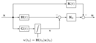
Figure 1: Block diagram of the proposed performance preserving integral control law (9) with tuning parameters $\mathbf{H}(t)$ and $\mathbf{K}_{\mathrm{I}}$, nominal state-feedback matrix $\mathbf{K}(t)$, and abbreviation $\mathbf{G}(t)$ given in (9c).

If the integrator’s initial condition is chosen as

$$\mathbf{v}(t_{0})=\mathbf{H}(t_{0})\mathbf{x}(t_{0}),$$ (10)

then the control law (9) preserves the performance of the nominal controller (4) in the unperturbed case; this is shown in the following proposition:

Proposition 11.

Consider the application of the control law (9) to the unperturbed plant, i.e., to (3a) with $\mathbf{w}(t)=\bm{0}$. If the inital conditions of $\mathbf{v}$ and $\mathbf{x}$ satisfy (10), then $\mathbf{u}(t)=-\mathbf{K}(t)\mathbf{x}(t)$ holds for all $t\geq t_{0}$.

The proof of Proposition 11 is given in Section 5.1.

Remark 12.

To see this result also intuitively, note that $\mathbf{G}(t)\mathbf{x}$ is the time derivative of $\mathbf{H}(t)\mathbf{x}$ along the plant’s trajectories for $\mathbf{u}=-\mathbf{K}(t)\mathbf{x}$ and $\mathbf{w}=\bm{0}$. Therefore, with proper initialization, $\mathbf{v}(t)=\mathbf{H}(t)\mathbf{x}$ holds for all $t\geq t_{0}$ in this case, and only the nominal control remains.

4.2 Stability Condition

In order to formulate a stability condition for the closed loop, the abbreviation

$$\mathbf{Q}(t)=\mathbf{H}(t)\mathbf{B}(t)$$ (11)

is introduced. Asymptotic stability of the overall closed loop may then be guaranteed using the following theorem, which is proven in Section 5.2.

Theorem 13.

Consider the control law (9) with a symmetric parameter matrix $\mathbf{K}_{\mathrm{I}}\in\mathbb{R}^{l\times l}$ and a uniformly bounded feedback matrix $\mathbf{H}(t)\in\mathbb{R}^{l\times n}$ with uniformly bounded time derivative $\dot{\mathbf{H}}(t)$. Let $\mathbf{Q}(t)$ be defined as in (11) and suppose that the nominal state feedback $\mathbf{K}(t)$ fulfills Assumption 6. If $\mathbf{Q}(t)+\mathbf{Q}(t)^{\mathrm{T}}$ is positive semidefinite for every $t$ and there exist positive constants $\alpha$, $\beta$, and a non-negative constant $T$ such that the inequalities

$$\lambda_{\mathrm{min}}(\mathbf{K}_{\mathrm{I}}) \geq\alpha,$$ (12a)

$$\int_{t_{0}}^{t_{0}+\tau}{{\lambda_{\mathrm{min}}\bigl{[}\mathbf{Q}(\sigma)+\mathbf{Q}(\sigma)^{\mathrm{T}}\bigr{]}}\,\mathrm{d}{\sigma}} \geq 2\beta\tau$$ (12b)

hold for all $t_{0}$ and all $\tau\geq T$, then the control law (9) asymptotically stabilizes the plant (3) for all perturbations that are asymptotically constant with respect to the control input in the sense of Definition 8.

The proof is given in Section 5.2.

Remark 14.

Note that the conditions on $\mathbf{K}_{\mathrm{I}}$ and $\mathbf{H}(t)$ are decoupled. Once a time-varying feedback matrix $\mathbf{H}(t)$ satisfying the conditions is fixed, the proposed control law asymptotically stabilizes the perturbed plant for every positive definite parameter matrix $\mathbf{K}_{\mathrm{I}}$.

Remark 15.

It is remarkable that the integral gain $\mathbf{K}_{\mathrm{I}}$ can in fact be chosen arbitrarily large, as long as it is positive definite. This is a consequence of the fact that it affects $\mathbf{v}-\mathbf{H}(t)\mathbf{x}$ rather than just the integral state $\mathbf{v}$; for positive definite $\mathbf{Q}(t)$ as in (11), the former is an output with relative degree one with respect to $\mathbf{u}$, which intuitively explains the lack of an upper bound for $\mathbf{K}_{\mathrm{I}}$.

The following corollary presents a useful candidate for the choice of the time-varying feedback matrix $\mathbf{H}(t)$ with a simplified (though slightly more conservative) stability condition. Further considerations and insights into the tuning of $\mathbf{H}(t)$ and $\mathbf{K}_{\mathrm{I}}$ are presented in Section 6.2.

Corollary 16.

Suppose that $\dot{\mathbf{B}}(t)$ is uniformly bounded. If the symmetric parameter matrix $\mathbf{K}_{\mathrm{I}}\in\mathbb{R}^{l\times l}$ and $\mathbf{B}(t)$ satisfy, for positive constants $\alpha$ and $\beta$, the conditions

$$\lambda_{\mathrm{min}}(\mathbf{K}_{\mathrm{I}}) \geq\alpha,$$ (13a)

$$\lambda_{\mathrm{min}}(\mathbf{B}(t)^{\mathrm{T}}\mathbf{B}(t)) \geq\beta$$ (13b)

for all $t$, then the control law (9) with $\mathbf{H}(t)=\mathbf{B}(t)^{\mathrm{T}}$ asymptotically stabilizes the plant (3) for all perturbations that are asymptotically constant with respect to the control input in the sense of Definition 8.

Remark 17.

Note that, for $\mathbf{H}(t)=\mathbf{B}(t)^{\mathrm{T}}$, the inequalities (13) imply conditions (12) of Theorem 13 with $T=0$ and the same constants $\alpha$, $\beta$.

4.3 Bounded-Input Bounded-State Stability

The previous considerations only guarantee stability for perturbations that are asymptotically constant with respect to the control input in the sense of Definition 8. For arbitrary perturbations, bounded-input bounded-state stability of the closed loop may be shown under the same conditions:

Theorem 18.

Consider the closed loop obtained by applying control law (9) to the plant (3). Suppose that the conditions of Theorem 13 are fulfilled; in particular, let system (5) be uniformly exponentially stable with positive constants $\mu$ and $M$ as in Definition 1 and let $B$, $F$, $H$ be uniform upper bounds for $\left\lVert\mathbf{B}(t)\right\rVert$, $\left\lVert\mathbf{F}(t)\right\rVert$, $\left\lVert\mathbf{H}(t)\right\rVert$, respectively. Then, the closed loop is uniformly bounded-input bounded-state stable with respect to the perturbation input $\mathbf{w}$. In particular, the controlled plant is also rendered uniformly bounded-input bounded-state stable with the gain

$$\gamma=\frac{BM}{\mu}\mathrm{e}^{\alpha\beta T}\sqrt{\frac{\lambda_{\mathrm{max}}(\mathbf{K}_{\mathrm{I}})}{\lambda_{\mathrm{min}}(\mathbf{K}_{\mathrm{I}})}}\frac{\lambda_{\mathrm{max}}(\mathbf{K}_{\mathrm{I}})}{\alpha}\frac{HF}{\beta}+\frac{FM}{\mu}.$$ (14)

The proof is given in Section 5.3.

5 Stability Analysis

In this section, the proposed approach for designing an integral controller is discussed in more detail. First, the closed-loop system is derived and the performance preserving property in Proposition 11 is shown. Stability is then analyzed, and the stability condition in Theorem 13 and the bounded-input bounded-state gain of Theorem 18 are proven.

5.1 Closed Loop System

In order to give a state-space representation of the closed loop, the state variable

$$\mathbf{z}=-\mathbf{K}_{\mathrm{I}}\mathbf{H}(t)\mathbf{x}+\mathbf{K}_{\mathrm{I}}\mathbf{v}+\mathbf{w}_{0}$$ (15)

with a constant vector $\mathbf{w}_{0}$ (to be defined later), and the abbreviation

$$\tilde{\mathbf{w}}(t)=\mathbf{F}(t)\mathbf{w}(t)-\mathbf{B}(t)\mathbf{w}_{0}$$ (16)

are introduced.

According to (3) and (9), the closed loop is then governed by

$$\dot{\mathbf{x}} =\bigl{[}\mathbf{A}(t)-\mathbf{B}(t)\mathbf{K}(t)\bigr{]}\mathbf{x}+\mathbf{B}(t)\mathbf{z}+\tilde{\mathbf{w}}$$ (17a)

$$\dot{\mathbf{z}} =-\mathbf{K}_{\mathrm{I}}\mathbf{H}(t)\bigl{[}\mathbf{B}(t)\mathbf{z}+\tilde{\mathbf{w}}\bigr{]}.$$ (17b)

In the unperturbed case, i.e., for $\mathbf{w}(t)=\mathbf{w}_{0}=\bm{0}$ and hence $\tilde{\mathbf{w}}(t)=\bm{0}$, the second of these equations reduces to

$$\dot{\mathbf{z}}=-\mathbf{K}_{\mathrm{I}}\mathbf{H}(t)\mathbf{B}(t)\mathbf{z},$$ (18)

and the control input is given by

$$\mathbf{u}=-\mathbf{K}(t)\mathbf{x}+\mathbf{z}.$$ (19)

Using these considerations, Proposition 11 may be proven.

Proof of Proposition 11: Initial condition (10) and $\mathbf{w}(t_{0})=\bm{0}$ imply $\mathbf{z}(t_{0})=\bm{0}$. Therefore, $\mathbf{z}(t)=\bm{0}$ is the unique solution of (18), and (19) yields $\mathbf{u}(t)=-\mathbf{K}(t)\mathbf{x}(t)$ for all $t\geq t_{0}$.  ∎

5.2 Asymptotic Stabilization

The stability of the closed-loop system is now studied for disturbances that are asymptotically constant with respect to the control input in the sense of Definition 8. To that end, the vector $\mathbf{w}_{0}$ in the closed-loop description is set to $\overline{\mathbf{w}}_{0}$ from that definition, and hence $\tilde{\mathbf{w}}(t)$ vanishes asymptotically.

Using (15) to obtain the representation (17) of this system preserves the closed-loop stability properties, if the associated state transformation

$$\begin{bmatrix}\mathbf{x}\\ \mathbf{z}\end{bmatrix}=\begin{bmatrix}\mathbf{I}&\bm{0}\\ -\mathbf{K}_{\mathrm{I}}\mathbf{H}(t)&\mathbf{K}_{\mathrm{I}}\end{bmatrix}\begin{bmatrix}\mathbf{x}\\ \mathbf{v}\end{bmatrix}+\begin{bmatrix}\bm{0}\\ \mathbf{w}_{0}\end{bmatrix}$$ (20)

is a Lyapunov transformation, i.e., if the transformation matrix

$$\mathbf{M}(t)=\begin{bmatrix}\mathbf{I}&\bm{0}\\ -\mathbf{K}_{\mathrm{I}}\mathbf{H}(t)&\mathbf{K}_{\mathrm{I}}\end{bmatrix}$$ (21)

has a uniformly bounded time derivative $\dot{\mathbf{M}}(t)$ and inverse $\mathbf{M}(t)^{-1}$, see e.g. (Adrianova, 1995, Chapter III). This is the case if $\dot{\mathbf{H}}$ is bounded and $\mathbf{K}_{\mathrm{I}}$ is invertible. As one can see from (17), closed-loop stability is then determined by the stability of the subsystem (17b) governing the state variable $\mathbf{z}$. Since it is excited by a vanishing disturbance, uniform exponential stability of its autonomous part guarantees its asymptotic stability. This yields the following intermediate result.

Lemma 19.

Consider the closed-loop system (16), (17) for disturbances $\mathbf{w}(t)$ that are asymptotically constant with respect to the control input in the sense of Definition 8. Suppose that the nominal state feedback $\mathbf{K}(t)$ fulfills Assumption 6 and that the system

$$\dot{\mathbf{z}}=-\mathbf{K}_{\mathrm{I}}\mathbf{H}(t)\mathbf{B}(t)\mathbf{z}$$ (22)

is uniformly exponentially stable. Then, the closed loop is asymptotically stable.

Proof 5.1.

Consider first system (17b), which governs the perturbed trajectories of $\mathbf{z}$. Since the corresponding unperturbed system (22) is uniformly exponentially stable, Lemma 2 along with $\lim_{t\to\infty}\tilde{\mathbf{w}}(t)=\bm{0}$ implies $\lim_{t\to\infty}\mathbf{z}(t)=\bm{0}$.

Interpret now the remaining system dynamics (17a) as a perturbed system with disturbances $\mathbf{z}(t)$ and $\tilde{\mathbf{w}}(t)$. Since both tend to zero asymptotically, and the unperturbed system is uniformly exponentially stable by virtue of Assumption 6, applying Lemma 2 again guarantees that also $\mathbf{x}(t)$ tends to zero asymptotically. This concludes the proof.

Verifying the condition of Lemma 19 is not easy in general. A more useful stability condition may be obtained by considering the function $V(\mathbf{z})=\mathbf{z}^{\mathrm{T}}\mathbf{P}\mathbf{z}$ with a positive definite matrix $\mathbf{P}$ as a quadratic candidate Lyapunov function for system (22). Its time derivative $\dot{V}$ along the trajectories of (22) is given by

$$\dot{V}(t,\mathbf{z})=-\mathbf{z}^{\mathrm{T}}\bigl{[}\mathbf{B}(t)^{\mathrm{T}}\mathbf{H}(t)^{\mathrm{T}}\mathbf{K}_{\mathrm{I}}^{\mathrm{T}}\mathbf{P}+\mathbf{P}\mathbf{K}_{\mathrm{I}}\mathbf{H}(t)\mathbf{B}(t)\bigr{]}\mathbf{z}.$$ (23)

One can see that by choosing $\mathbf{P}=\mathbf{K}_{\mathrm{I}}^{-1}$ and selecting the controller parameter $\mathbf{K}_{\mathrm{I}}$ as a symmetric, positive definite matrix, the resulting stability condition for $\mathbf{H}(t)$ can be decoupled from $\mathbf{K}_{\mathrm{I}}$. Using these considerations, Theorem 13 can now be proven.

Proof of Theorem 13: In order to show uniform exponential stability of system (22), the Lyapunov function candidate $V(\mathbf{z})=\mathbf{z}^{\mathrm{T}}\mathbf{K}_{\mathrm{I}}^{-1}\mathbf{z}$ is considered. Its time derivative $\dot{V}$ along the trajectories of (22) satisfies

$$\dot{V}(t,\mathbf{z}) =-\mathbf{z}^{\mathrm{T}}\bigl{[}\mathbf{H}(t)\mathbf{B}(t)+\mathbf{B}(t)^{\mathrm{T}}\mathbf{H}(t)^{\mathrm{T}}\bigr{]}\mathbf{z}$$

$$\leq-\lambda_{\mathrm{min}}\bigl{[}\mathbf{H}(t)\mathbf{B}(t)+\mathbf{B}(t)^{\mathrm{T}}\mathbf{H}(t)^{\mathrm{T}}\bigr{]}\mathbf{z}^{\mathrm{T}}\mathbf{z}.$$ (24)

Introducing $\gamma(t)=\lambda_{\mathrm{min}}\bigl{[}\mathbf{H}(t)\mathbf{B}(t)+\mathbf{B}(t)^{\mathrm{T}}\mathbf{H}(t)^{\mathrm{T}}\bigr{]}\geq 0$ as an abbreviation and using $\mathbf{z}^{\mathrm{T}}\mathbf{K}_{\mathrm{I}}^{-1}\mathbf{z}\leq\lambda_{\mathrm{max}}(\mathbf{K}_{\mathrm{I}}^{-1})\mathbf{z}^{\mathrm{T}}\mathbf{z}$, one has

$$\dot{V}(t,\mathbf{z}) \leq-\frac{\gamma(t)}{{\lambda_{\mathrm{max}}(\mathbf{K}_{\mathrm{I}}^{-1})}}V(\mathbf{z})\leq-\alpha\gamma(t)V(\mathbf{z}).$$ (25)

Integrating this inequality yields

$$V(\mathbf{z}(t))\leq\exp\Bigl{(}-\alpha\int_{t_{0}}^{t}{{\gamma(\sigma)}\,\mathrm{d}{\sigma}}\Bigr{)}V(\mathbf{z}(t_{0})).$$ (26)

According to (12b), $\gamma$ satisfies

$$\int_{t_{0}}^{t}{{\gamma(\sigma)}\,\mathrm{d}{\sigma}}\geq\begin{cases}0&t-t_{0}<T\\ 2\beta(t-t_{0})&t-t_{0}\geq T.\end{cases}$$ (27)

Thus,

$$\int_{t_{0}}^{t}{{\gamma(\sigma)}\,\mathrm{d}{\sigma}}\geq 2\beta(t-t_{0})-2\beta T$$ (28)

holds in either of the two cases, and substitution into (26) yields

$$V(\mathbf{z}(t))\leq\mathrm{e}^{2\alpha\beta T}\mathrm{e}^{-2\alpha\beta(t-t_{0})}V(\mathbf{z}(t_{0})).$$ (29)

Since $\lambda_{\mathrm{min}}(\mathbf{K}_{\mathrm{I}}^{-1})\left\lVert\mathbf{z}\right\rVert^{2}\leq V(\mathbf{z})\leq\lambda_{\mathrm{max}}(\mathbf{K}_{\mathrm{I}}^{-1})\left\lVert\mathbf{z}\right\rVert^{2}$ holds, one obtains

$$\left\lVert\mathbf{z}(t)\right\rVert\leq\mathrm{e}^{\alpha\beta T}\sqrt{\frac{\lambda_{\mathrm{max}}(\mathbf{K}_{\mathrm{I}})}{\lambda_{\mathrm{min}}(\mathbf{K}_{\mathrm{I}})}}\mathrm{e}^{-\alpha\beta(t-t_{0})}\left\lVert\mathbf{z}(t_{0})\right\rVert.$$ (30)

This shows uniform exponential stability of system (22), and the proof is concluded by applying Lemma 19.  ∎

5.3 Bounded-Input Bounded-State Stability Gain

In order to analyze the behavior for general disturbances, the closed loop is now studied for $\mathbf{w}_{0}=\bm{0}$, i.e., with $\tilde{\mathbf{w}}=\mathbf{F}(t)\mathbf{w}$. Theorem 18 may then be proven.

Proof of Theorem 18: In the unperturbed case, i.e., $\tilde{\mathbf{w}}=\bm{0}$, the closed-loop system (17) is uniformly exponentially stable. This follows from (Zhou, 2016, Theorem 2) because (5) and (18) are uniformly exponentially stable and (17) is in block triangular form. According to (Rugh, 1995, Lemma 12.4), this guarantees uniform bounded-input bounded-state stability. The gain $\gamma$ for the closed-loop plant states as stated in (14) will be derived in the following.

Let $\bm{\Phi}(t,t_{0})$ and $\bm{\Phi}_{\mathrm{z}}(t,t_{0})$ denote the state transition matrices of (5) and (18), respectively. Bounds for these transition matrices are given by

$$\left\lVert\bm{\Phi}(t,t_{0})\right\rVert \leq Me^{-\mu(t-t_{0})}\quad\text{ and }$$ (31a)

$$\left\lVert\bm{\Phi}_{\mathrm{z}}(t,t_{0})\right\rVert \leq M_{\mathrm{z}}e^{-\mu_{\mathrm{z}}(t-t_{0})}$$ (31b)

with $M,\,\mu>0$ as in the theorem and $\mu_{\mathrm{z}}=\alpha\beta$ and $M_{\mathrm{z}}=\mathrm{e}^{\alpha\beta T}\sqrt{\frac{\lambda_{\mathrm{max}}(\mathbf{K}_{\mathrm{I}})}{\lambda_{\mathrm{min}}(\mathbf{K}_{\mathrm{I}})}}$, obtained from (30).

For a general perturbation $\mathbf{w}(t)$ and with $\mathbf{w}_{0}=\bm{0}$, the effect of the input $\mathbf{w}(t)$ on $\mathbf{z}(t)$ (with $\mathbf{z}(t_{0})=\bm{0}$) in system (22) is given by

$$\mathbf{z}(t)=-\int_{t_{0}}^{t}{{\bm{\Phi}_{\mathrm{z}}(t,\tau)\mathbf{K}_{\mathrm{I}}\mathbf{H}(\tau)\mathbf{F}(\tau)\mathbf{w}(\tau)}\,\mathrm{d}{\tau}}.$$ (32)

Using the upper bounds $B,H,F$ for $\mathbf{B}(t),\mathbf{H}(t),\mathbf{F}(t)$, one obtains the bound

$$\|\mathbf{z}(t)\| \leq\int_{t_{0}}^{t}{{M_{\mathrm{z}}e^{-\mu_{\mathrm{z}}(t-\tau)}\left\lVert\mathbf{K}_{\mathrm{I}}\right\rVert HF}\,\mathrm{d}{\tau}}\sup_{\tau\in[t_{0},t]}\left\lVert\mathbf{w}(\tau)\right\rVert$$

$$\leq\frac{M_{\mathrm{z}}}{\mu_{\mathrm{z}}}HF\lambda_{\mathrm{max}}(\mathbf{K}_{\mathrm{I}})\sup_{\tau\in[t_{0},t]}\left\lVert\mathbf{w}(\tau)\right\rVert.$$ (33)

The zero state response of the plant state $\mathbf{x}(t)$ can be stated as

$$\mathbf{x}(t)=\int_{t_{0}}^{t}{{\bm{\Phi}(t,\tau)\mathbf{B}(\tau)\mathbf{z}(\tau)}\,\mathrm{d}{\tau}}+\int_{t_{0}}^{t}{{\bm{\Phi}(t,\tau)\mathbf{F}(\tau)\mathbf{w}(\tau)}\,\mathrm{d}{\tau}}.$$ (34)

Performing estimates analogous to (5.3) and using this bound in (34) results in

$$\|\mathbf{x}(t)\| \leq\frac{BM}{\mu}\frac{M_{\mathrm{z}}}{\mu_{\mathrm{z}}}HF\lambda_{\mathrm{max}}(\mathbf{K}_{\mathrm{I}})\sup_{\tau\in[t_{0},t]}\left\lVert\mathbf{w}(\tau)\right\rVert$$

$$\quad+\frac{FM}{\mu}\sup_{\tau\in[t_{0},t]}\left\lVert\mathbf{w}(\tau)\right\rVert.$$ (35)

Taking the supremum on the left hand side over $t\geq t_{0}$ shows that the controlled plant is uniformly bounded-input bounded-state stable with gain (14).  ∎

6 Implementation Issues

This section discusses two practical aspects of the proposed control law: the mitigation of integrator windup and the choice of parameters.

6.1 Mitigation of Windup

In the presence of control input saturation, controllers with integral feedback are known to suffer from an effect called controller windup, see e.g. Hippe (2006). While the control input is saturated, the internal state of the controller may wind up, causing large, undesired overshoots or even unbounded trajectories. This section presents a way to mitigate this problem for the proposed control law.

Suppose that the control input, which is actually applied to the plant, is given by $\mathbf{u}^{*}$ rather than $\mathbf{u}$. The signal $\mathbf{u}^{*}$ may be obtained from $\mathbf{u}$, for example, by component-wise saturation functions. Here, the only assumption made about $\mathbf{u}^{*}$ is that $\mathbf{u}^{*}=\mathbf{u}$, when $\mathbf{u}$ satisfies the control input constraints.

In order to avoid windup, the control law (9) may be modified as

$$\mathbf{u} =-\bigl{[}\mathbf{K}(t)+\mathbf{K}_{\mathrm{I}}\mathbf{H}(t)\bigr{]}\mathbf{x}+\mathbf{K}_{\mathrm{I}}\mathbf{v}$$ (36a)

$$\dot{\mathbf{v}} =\mathbf{G}(t)\mathbf{x}+\mathbf{H}(t)\mathbf{B}(t)(\mathbf{u}^{*}-\mathbf{u}).$$ (36b)

Fig. 2 depicts a block diagram of this modified control law. It is motivated by the desire to maintain the property pointed out in Remark 12 also in the case $\mathbf{u}\neq\mathbf{u}^{*}$: that the right-hand side of $\dot{\mathbf{v}}$ stays equal to the time derivative of $\mathbf{H}(t)\mathbf{x}$.

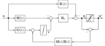
Figure 2: Block diagram of the proposed performance preserving integral control law with anti-windup (36), assuming a saturation nonlinearity between unconstrained control input $\mathbf{u}$ and constrained control input $\mathbf{u}^{*}$.

With this modification, the following asymptotic property of $\mathbf{u}(t)$ can be shown for the constrained closed loop.

Proposition 20.

Consider the plant (3) with the unconstrained control input $\mathbf{u}$ replaced by a constrained input $\mathbf{u}^{*}$. If the conditions of Theorem 13 are fulfilled, then the unconstrained control input $\mathbf{u}(t)$ obtained with the control law (36), (9c) satisfies

$$\lim_{t\to\infty}\mathbf{u}(t)+\mathbf{K}(t)\mathbf{x}(t)+\mathbf{w}(t)=\bm{0},$$ (37)

i.e., $\mathbf{u}(t)$ asymptotically tends to $-\mathbf{K}(t)\mathbf{x}(t)-\mathbf{w}(t)$.

Proof 6.1.

One may verify that after the replacement of $\mathbf{u}$ by $\mathbf{u}^{*}$ in (3) and of (9b) by (36b), the variable $\mathbf{z}$ defined in (15) still satisfies (17b). Therefore, the proof of Theorem 13 is applicable without modification to show that $\mathbf{z}(t)$ tends to zero. Noting that $\mathbf{z}(t)=\mathbf{u}(t)+\mathbf{K}(t)\mathbf{x}(t)+\mathbf{w}(t)-\tilde{\mathbf{w}}(t)$ and that $\tilde{\mathbf{w}}(t)$ tends to zero completes the proof.

Remark 21.

Note that although the nominal control signal with a disturbance compensation is recovered asymptotically, plant windup or the directionality problem may additionally occur in the presence of input saturation, see, e.g. Hippe (2006). Therefore, no general formal statements about closed-loop stability in the presence of saturation nonlinearities can be made, but controller windup of the integrator is prevented.

Remark 22.

From this proof and from (22), one can see that nominal behavior is approached the faster, the larger $\mathbf{K}_{\mathrm{I}}$ is. Hence, also in the perturbed case, nominal performance is recovered with increasing integrator gain.

6.2 Tuning of Parameters

This section discusses some guidelines for the choices of $\mathbf{K}_{\mathrm{I}}$ and $\mathbf{H}(t)$. Regarding $\mathbf{K}_{\mathrm{I}}$, one can see from the proofs in the previous section, in particular from (30), that the exponential convergence rate $\mu$ in the sense of Definition 1 is given by $\mu=\alpha\beta$ with the positive constants $\alpha$ and $\beta$ from Theorem 13. Along with that theorem’s conditions, this suggests that a desired convergence rate $\mu^{*}$ can be ensured by selecting the positive definite controller parameter $\mathbf{K}_{\mathrm{I}}$ such that $\lambda_{\mathrm{min}}(\mathbf{K}_{\mathrm{I}})\geq\frac{\mu^{*}}{\beta}.$

As pointed out in Corollary 16, one possible choice for $\mathbf{H}(t)$ is $\mathbf{H}(t)=\mathbf{B}(t)^{\mathrm{T}}$. As pointed out in Remark 17, $\beta$ has the same meaning as in Theorem 13 in this case, i.e., it may be used for tuning $\mathbf{K}_{\mathrm{I}}$ as discussed before. Under conditions of the corollary, $\mathbf{H}(t)$ may also be chosen as

$$\mathbf{H}(t)=\frac{\mathbf{B}(t)^{\mathrm{T}}}{\left\lVert\mathbf{B}(t)\right\rVert^{2}}\quad\text{or}\quad\mathbf{H}(t)=\frac{\mathbf{B}(t)^{\mathrm{T}}}{\lambda_{\mathrm{min}}(\mathbf{B}(t)^{\mathrm{T}}\mathbf{B}(t))}.$$ (38)

The latter choice, in particular, achieves

$$\int_{t_{0}}^{t_{0}+\tau}{{\lambda_{\mathrm{min}}\bigl{[}\mathbf{Q}(\sigma)+\mathbf{Q}(\sigma)^{\mathrm{T}}\bigr{]}}\,\mathrm{d}{\sigma}}=2\tau$$ (39)

for all $\tau\geq 0$ and $t_{0}$, i.e., equality is obtained in condition (12b) of Theorem 13 with $\beta=1$, which yields the convergence rate $\mu=\lambda_{\mathrm{min}}(\mathbf{K}_{\mathrm{I}})$.

If $\left\lVert\mathbf{B}(t)\right\rVert$ or $\lambda_{\mathrm{min}}(\mathbf{B}(t)^{\mathrm{T}}\mathbf{B}(t))$ is not uniformly bounded from below by a positive constant, choosing $\mathbf{H}(t)$ is less straightforward. In this case, the choice $\mathbf{H}(t)=\mathbf{B}(t)^{\mathrm{T}}$ or variants of (38) such as

$$\mathbf{H}(t)=\frac{\mathbf{B}(t)^{\mathrm{T}}}{\max(\lambda_{\mathrm{min}}(\mathbf{B}(t)^{\mathrm{T}}\mathbf{B}(t)),L)}$$ (40)

with $L>0$ may be explored, but in general $\mathbf{H}(t)$ has to be chosen in accordance with the conditions of Theorem 13, which have be checked on a case-to-case basis.

7 Special Cases

This section discusses two important special cases of the controller whose general form is given in (9): the design of a (time-varying) output integral feedback, and the design for a time-invariant plant.

7.1 Output-Feedback Integral Action

In practice, it is sometimes desired that the integral controller should be designed using the integral of a given output $\mathbf{y}$. The problem then becomes that of finding a time-varying gain $\mathbf{M}(t)$ and a state-feedback gain $\mathbf{H}(t)$ such that the control law (9) may be written as

$$\mathbf{u} =-\bigl{[}\mathbf{K}(t)+\mathbf{K}_{\mathrm{I}}\mathbf{H}(t)\bigr{]}\mathbf{x}+\mathbf{K}_{\mathrm{I}}\mathbf{v}$$ (41a)

$$\dot{\mathbf{v}} =\mathbf{M}(t)\mathbf{y},$$ (41b)

i.e., such that $\mathbf{G}(t)=\mathbf{M}(t)\mathbf{C}(t)$ holds in (9) for all $t$. To fulfill (9c), $\mathbf{H}(t)$ then has to be a solution of the system

$$\dot{\mathbf{H}} =-\mathbf{H}\bigl{[}\mathbf{A}(t)-\mathbf{B}(t)\mathbf{K}(t)\bigr{]}+\mathbf{M}\mathbf{C}(t),$$ (42a)

$$\mathbf{Q} =\mathbf{H}\mathbf{B}(t).$$ (42b)

Therein, $\mathbf{M}\in\mathbb{R}^{l\times m}$ acts as an input, $\mathbf{H}\in\mathbb{R}^{l\times n}$ is the (matrix-valued) state, and the output $\mathbf{Q}\in\mathbb{R}^{l\times l}$ is relevant for the stability condition in Theorem 13.

Finding a solution for this system can be interpreted as a control problem for the dual of the nominal closed loop. To see this, the $i$-th rows of $\mathbf{H}$, $\mathbf{M}$, and $\mathbf{Q}$ are denoted by $\mathbf{h}_{i}\in\mathbb{R}^{n}$, $\mathbf{m}_{i}\in\mathbb{R}^{m}$, and $\mathbf{q}_{i}\in\mathbb{R}^{l}$, respectively, i.e.,

$$\mathbf{H}=\begin{bmatrix}\mathbf{h}_{1}^{\mathrm{T}}\\ \vdots\\ \mathbf{h}_{l}^{\mathrm{T}}\end{bmatrix},\quad\mathbf{M}=\begin{bmatrix}\mathbf{m}_{1}^{\mathrm{T}}\\ \vdots\\ \mathbf{m}_{l}^{\mathrm{T}}\end{bmatrix},\quad\mathbf{Q}=\begin{bmatrix}\mathbf{q}_{1}^{\mathrm{T}}\\ \vdots\\ \mathbf{q}_{l}^{\mathrm{T}}\end{bmatrix}.$$ (43)

Substitution into (42) shows that the transposed rows are governed by the system

$$\dot{\mathbf{h}}_{i} =-\bigl{[}\mathbf{A}(t)-\mathbf{B}(t)\mathbf{K}(t)\bigr{]}^{\mathrm{T}}\mathbf{h}_{i}+\mathbf{C}(t)^{\mathrm{T}}\mathbf{m}_{i}$$ (44a)

$$\mathbf{q}_{i} =\mathbf{B}(t)^{\mathrm{T}}\mathbf{h}_{i}.$$ (44b)

This system is the dual of the nominal closed loop. It is therefore anti-stable, i.e., uniformly exponentially stable in reverse time. For bounded $\mathbf{m}_{i}(t)$, the existence of bounded solutions is guaranteed from the fact that the system has an exponential dichotomy, see, e.g., (Coppel, 1978, Ch. 3, Proposition 2). Depending on the structure of the system, such solutions with desired $\mathbf{Q}(t)$ may be found, for example, using flatness-based or input-output linearization techniques.

Remark 23.

Note that although the integral (41b) is computed only from the output, the overall control law (41) still requires full-state feedback. To obtain a pure output feedback controller, an unknown input observer may be used to reconstruct the state $\mathbf{x}$ from the measured output $\mathbf{y}$ without knowledge of the disturbance $\mathbf{w}$, see e.g. Ichalal and Mammar (2015); Tranninger et al. (2021).

7.2 Time-Invariant Case

Consider the time-invariant case, i.e., a time-invariant plant $\dot{\mathbf{x}}=\mathbf{A}\mathbf{x}+\mathbf{B}\mathbf{u}$ and nominal control law $\mathbf{u}=-\mathbf{K}\mathbf{x}$. Then, the gain matrices $\mathbf{H}$ and $\mathbf{G}$ may also be chosen to be constant. Considering, in particular, the output-feedback case, one may choose $\mathbf{G}=\mathbf{M}\mathbf{C}$ with constant matrix $\mathbf{M}$ and compute $\mathbf{H}$ according to (9c) as

$$\mathbf{H}=\mathbf{G}(\mathbf{A}-\mathbf{B}\mathbf{K})^{-1}=\mathbf{M}\mathbf{C}(\mathbf{A}-\mathbf{B}\mathbf{K})^{-1}.$$ (45)

In this case, the control law (41) becomes

$$\mathbf{u} =-\Bigl{[}\mathbf{K}+\mathbf{K}_{\mathrm{I}}\mathbf{M}\mathbf{C}(\mathbf{A}-\mathbf{B}\mathbf{K})^{-1}\Bigr{]}\mathbf{x}+\mathbf{K}_{\mathrm{I}}\mathbf{v}$$ (46a)

$$\dot{\mathbf{v}} =\mathbf{M}\mathbf{y}.$$ (46b)

A reasonable choice for the constant matrix $\mathbf{M}\in\mathbb{R}^{l\times m}$ is given by the following proposition, which is a generalization of (Seeber and Moreno, 2020, Proposition 1) to the multivariable case.

Proposition 24.

Consider the closed loop formed by applying the control law (46) to the time-invariant plant $\dot{\mathbf{x}}=\mathbf{A}\mathbf{x}+\mathbf{B}\mathbf{u}$, $\mathbf{y}=\mathbf{C}\mathbf{x}$ and suppose that the matrix $\mathbf{A}-\mathbf{B}\mathbf{K}$ is Hurwitz. If $\mathbf{C}(\mathbf{A}-\mathbf{B}\mathbf{K})^{-1}\mathbf{B}$ is left-invertible and $\mathbf{M}$ is the corresponding left (pseudo-)inverse

$$\mathbf{M}=\bigl{[}\mathbf{C}(\mathbf{A}-\mathbf{B}\mathbf{K})^{-1}\mathbf{B}\bigr{]}^{+},$$ (47)

then the closed-loop eigenvalues are given by the union of the eigenvalues of the matrices $\mathbf{A}-\mathbf{B}\mathbf{K}$ and $-\mathbf{K}_{\mathrm{I}}$.

Proof 7.1.

With the considered value of $\mathbf{M}$ and taking into account (45), one has $\mathbf{H}\mathbf{B}=\mathbf{M}\mathbf{C}(\mathbf{A}-\mathbf{B}\mathbf{K})^{-1}\mathbf{B}=\mathbf{I}$. The unperturbed closed-loop system (17) hence is

$$\begin{bmatrix}\dot{\mathbf{x}}\\ \dot{\mathbf{z}}\end{bmatrix} =\begin{bmatrix}\mathbf{A}-\mathbf{B}\mathbf{K}&\mathbf{B}\\ \bm{0}&-\mathbf{K}_{\mathrm{I}}\end{bmatrix}\begin{bmatrix}\mathbf{x}\\ \mathbf{z}\end{bmatrix}.$$ (48)

The claimed statement is then obvious from the system’s block triangular structure.

Remark 25.

The performance preserving effect of the proposed controller, which is achieved by selecting the initial value according to Proposition 11 as

$$\mathbf{v}(t_{0})=\mathbf{M}\mathbf{C}(\mathbf{A}-\mathbf{B}\mathbf{K})^{-1}\mathbf{x}(t_{0}),$$ (49)

can here also be seen from the fact that the controller preserves the nominal closed-loop eigenvalues, while the additional eigenvalues may be tuned using $\mathbf{K}_{\mathrm{I}}$.

Remark 26.

Note that invertibility of $\mathbf{C}(\mathbf{A}-\mathbf{B}\mathbf{K})^{-1}\mathbf{B}$ is a reasonable assumption, because it is equivalent to the absence of transmission zeros in the plant at zero, i.e., to a non-singular dc-gain.

8 Simulation Example

The presented approach is demonstrated in a simulation using a two-tank system as considered, e.g., in Pan et al. (2005). The plant is goverened by the nonlinear model $\dot{z}_{1}=-c_{1}\sqrt{z_{1}}+c_{3}q+w$, $\dot{z}_{2}=c_{1}\sqrt{z_{1}}-c_{2}\sqrt{z_{2}}$ with measured liquid levels $z_{1},z_{2}$, pump voltage $q$, disturbance $w$, and positive parameters $c_{1},c_{2},c_{3}$. The goal is for the lower tank level $z_{2}$ to track a given reference $r(t)=c_{4}+c_{5}\sin(2\pi c_{6}t)$ with positive constants $c_{4}\geq c_{5}$ and $c_{6}$. For control design, the system is linearized along the reference trajectory $z_{\mathrm{ref},1}(t)=c_{1}^{-2}(c_{2}\sqrt{r(t)}+\dot{r}(t))^{2}$, $z_{\mathrm{ref},2}(t)=r(t)$, see, e.g., (Rudolph, 2021, Chapter 5.2) or (Shao and Wang, 2014), and the control input is chosen as $q=u+q_{\mathrm{ref}}(t)$ with $q_{\mathrm{ref}}(t)=c_{3}^{-1}\dot{z}_{\mathrm{ref},1}(t)+c_{1}c_{3}^{-1}\sqrt{z_{\mathrm{ref},1}(t)}$ to obtain the linear, time-varying dynamics in form (3a)

$$\dot{\mathbf{x}}=\begin{bmatrix}-\frac{c_{1}}{2\sqrt{z_{\mathrm{ref},1}(t)}}&0\\ \frac{c_{1}}{2\sqrt{z_{\mathrm{ref},1}(t)}}&-\frac{c_{2}}{2\sqrt{z_{\mathrm{ref},2}(t)}}\\ \end{bmatrix}\mathbf{x}+\begin{bmatrix}c_{3}\\ 0\end{bmatrix}u+\begin{bmatrix}1\\ 0\end{bmatrix}w$$ (50)

for the linearized tracking error $\mathbf{x}=\mathbf{z}-\mathbf{z}_{\mathrm{ref}}(t)$. The model parameters $c_{1},c_{2},c_{3}$ are taken from the experimental setup in (Pan et al., 2005); Table 1 lists them along with parameters $c_{4},c_{5},c_{6}$ of the reference.

Due to the lower triangular structure and the chosen reference, system (50) can be shown to be UES for $u=w=0$, see (Zhou, 2016, Lemma 5 & Theorem 2). Hence, the nominal state feedback $\mathbf{K}(t)=\bm{0}$ is used in the simulation example for simplicity. Choosing, furthermore, $\mathbf{H}(t)=[\alpha\quad\alpha]$ with constant $\alpha>0$, computing $\mathbf{G}(t)$ from (9c) and (50), and taking into account the linearization, relation (36) yields the overall control law

$$q =q_{\mathrm{ref}}(t)-k_{\mathrm{I}}\alpha(z_{1}-z_{\mathrm{ref},1}(t)+z_{2}-z_{\mathrm{ref},2}(t))+k_{\mathrm{I}}v,$$

$$\dot{v} =-\frac{\alpha c_{2}}{2\sqrt{z_{\mathrm{ref},2}(t)}}(z_{2}-z_{\mathrm{ref},2}(t))+\alpha c_{3}(q^{*}-q)$$ (51)

where $u^{*}=q^{*}-q_{\mathrm{ref}}(t)$ is substituted in (36), and $q^{*}=\max(0,\min(Q,q))$ denotes the saturated input which is applied to the plant ($Q$ is a positive parameter).

Table 1: Parameters of the simulation model

$c_{1}$	$0.513\text{\,}\sqrt{cm}\mathrm{/}\mathrm{s}$	$c_{2}$	$0.513\text{\,}\sqrt{cm}\mathrm{/}\mathrm{s}$
$c_{3}$	$0.299\text{\,}\mathrm{c}\mathrm{m}\mathrm{/}\mathrm{V}\mathrm{s}$	$c_{4}$	$7\text{\,}\mathrm{c}\mathrm{m}$
$c_{5}$	$2\text{\,}\mathrm{c}\mathrm{m}$	$c_{6}$	$0.008\text{\,}\mathrm{H}\mathrm{z}$

Fig. 3 compares the tracking performance obtained with the proposed controller to that of a standard I-controller

$$q=q_{\mathrm{ref}}(t)+k_{\mathrm{I}}v,\qquad\dot{v}=-\beta(z_{2}-z_{\mathrm{ref},2}(t))$$ (52)

with constant positive parameters $k_{\mathrm{I}}$ and $\beta$. For the simulation, the nonlinear plant is used with constant disturbance $w=$0.5\text{\,}\mathrm{c}\mathrm{m}\mathrm{/}\mathrm{s}$$, saturation limit $Q=$8\text{\,}\mathrm{V}$$ and initial conditions $\mathbf{z}(0)=\bm{0}$, $v(0)=0$. For comparison purposes, the constants $\alpha=0.12$, $\beta=0.0062$ are chosen to obtain a similar settling time (to within $2\text{\,}\mathrm{\char 37\relax}$ of the reference) with both controllers for $k_{\mathrm{I}}=1$. One can see that, with increasing $k_{\mathrm{I}}$, performance improves with the proposed controller, whereas the I-controller tends to oscillations. As a result, the proposed controller achieves superior tracking, and its performance is insensitive even to fairly large gains $k_{\mathrm{I}}$. For $k_{\mathrm{I}}=10$, the proposed controller is moreover simulated with and without anti-windup for comparison, demonstrating also the practical usefulness of the proposed anti-windup strategy in the form of a reduced overshoot.

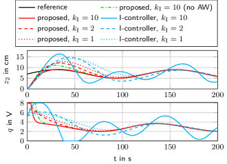
Figure 3: Simulated liquid level $z_{2}$ of the second tank along with its reference, and pump voltage $q$. Results obtained with the proposed controller (8) and with a standard I-controller are shown, for different values of the integral gain $k_{\mathrm{I}}$ and in one case with disabled anti-windup (AW).

9 Conclusion and Outlook

An approach for adding integral action to a given state-feedback controller for a linear, time-varying, multivariable plant was proposed. With proper initialization of the integrator, performance of the nominal state feedback is preserved in the unperturbed case and, asymptotically, also with increasing integrator gain. Additionally, in the time-invariant case, all nominal closed-loop eigenvalues are preserved.

Conditions were derived that allow to guarantee stability for any positive definite integrator gain; specifically, bounded-input bounded-state stability for any disturbance as well as asymptotic stability for perturbations, whose action on the plant is constant with respect to the control input, was shown. To facilitate the practical implementation of the controller, tuning guidelines and a scheme to mitigate windup were discussed.

Future work may focus on further investigating the case of using only the integral of a given output to construct the controller, i.e., the design of an output-feedback integral action. As shown, this case requires to invert the dual of the nominal closed loop in such a way that the integral of its output is positive definite. Achieving this in the general case, without relying on flatness or related properties, would be an interesting problem to be studied. Furthermore, the use of estimated rather than directly measured plant states and the corresponding disturbance rejection properties may also be investigated.

References

- Adrianova (1995) Adrianova, L.Y., 1995. Introduction to Linear Systems of Differential Equations (Translations of Mathematical Monographs). American Mathematical Society.
- Anderson et al. (2013) Anderson, B.D.O., Ilchmann, A., Wirth, F.R., 2013. Stabilizability of linear time-varying systems. Systems & Control Letters 62, 747–755.
- Athans and Falb (2013) Athans, M., Falb, P.L., 2013. Optimal Control: An Introduction to the Theory and its Applications. Courier Corporation.
- Attia et al. (2020) Attia, M.S., Bouafoura, M.K., Braiek, N.B., 2020. Decentralized suboptimal state feedback integral tracking control design for coupled linear time-varying systems. Mathematical Problems in Engineering 2020. doi:10.1155/2020/7519014.
- Babiarz et al. (2021) Babiarz, A., Cuong, L.V., Czornik, A., Doan, T.S., 2021. Necessary and sufficient conditions for assignability of dichotomy spectrum of one-sided discrete time-varying linear systems. IEEE Transactions on Automatic Control doi:10.1109/TAC.2021.3073061.
- Bakhshande and Söffker (2015) Bakhshande, F., Söffker, D., 2015. Proportional-integral-observer: A brief survey with special attention to the actual methods using ACC benchmark, in: 8th Vienna International Conference on Mathematical Modelling, pp. 532–537.
- Chen et al. (2020) Chen, L., Edwards, C., Alwi, H., 2020. Sliding mode observers for a class of linear parameter varying systems. International Journal of Robust and Nonlinear Control 30, 3134–3148. doi:10.1002/rnc.4951.
- Chen et al. (2016) Chen, W.H., Yang, J., Guo, L., Li, S., 2016. Disturbance-observer-based control and related methods – an overview. IEEE Transactions on Industrial Electronics 63, 1083–1095.
- Coppel (1978) Coppel, W.A., 1978. Dichotomies in Stability Theory. Springer, Berlin, Germany.
- Do et al. (2020) Do, M.H., Koenig, D., Theilliol, D., 2020. Robust H∞ proportional-integral observer-based controller for uncertain LPV system. Journal of the Franklin Institute 357, 2099–2130. doi:10.1016/j.jfranklin.2019.11.053.
- Franklin et al. (1986) Franklin, G.F., Powell, J.D., Emami-Naeini, A., 1986. Feedback Control of Dynamic Systems. Addison-Wesley.
- Hahn (1967) Hahn, W., 1967. Stability of Motion. Springer, Berlin, Germany.
- Hippe (2006) Hippe, P., 2006. Windup in Control. Springer.
- Ichalal and Mammar (2015) Ichalal, D., Mammar, S., 2015. On unknown input observers for LPV systems. IEEE Transactions on Industrial Electronics 62, 5870–5880. doi:10.1109/tie.2015.2448055.
- Kaczorek (1979) Kaczorek, T., 1979. Proportional-integral observers for linear multivariable time-varying systems. at–Automatisierungstechnik 27, 359–363.
- Kaczorek (1980) Kaczorek, T., 1980. Reduced-order proportional-integral observers for linear multivariable time-varying systems. at - Automatisierungstechnik 28. doi:10.1524/auto.1980.28.112.164.
- Kalman (1960) Kalman, R.E., 1960. Contributions to the theory of optimal control. Boletin de la Sociedad Matematica Mexicana 5, 102–119.
- Palanki and Kravaris (1997) Palanki, S., Kravaris, C., 1997. Controller synthesis for time-varying systems by input/output linearization. Computers & Chemical Engineering 21, 891–903.
- Pan et al. (2005) Pan, H., Wong, H., Kapila, V., de Queiroz, M.S., 2005. Experimental validation of a nonlinear backstepping liquid level controller for a state coupled two tank system. Control Engineering Practice 13, 27–40.
- Qiu et al. (2019) Qiu, B., Wang, G., Fan, Y., Mu, D., Sun, X., 2019. Robust path-following control based on trajectory linearization control for unmanned surface vehicle with uncertainty of model and actuator saturation. IEEJ Transactions on Electrical and Electronic Engineering 14, 1681–1690. doi:10.1002/tee.22991.
- Rudolph (2021) Rudolph, J., 2021. Flatness-Based Control. Shaker, Düren, Germany. doi:10.2370/9783844078930.
- Rugh (1995) Rugh, W.J., 1995. Linear System Theory, 2nd Edition. Pearson.
- Sariyildiz et al. (2020) Sariyildiz, E., Oboe, R., Ohnishi, K., 2020. Disturbance observer-based robust control and its applications: 35th anniversary overview. IEEE Transactions on Industrial Electronics 67, 2042–2053.
- Seeber and Moreno (2020) Seeber, R., Moreno, J.A., 2020. Performance preserving integral extension of linear and homogeneous state-feedback controllers, in: 21st IFAC World Congress, Berlin, Germany (virtual). pp. 5203–5208. doi:10.1016/j.ifacol.2020.12.1150.
- Shafai and Carroll (1985) Shafai, B., Carroll, R.L., 1985. Design of proportional-integral observer for linear time-varying multivariable systems, in: 24th IEEE Conference on Decision and Control, pp. 597–599.
- Shao and Wang (2014) Shao, X., Wang, H., 2014. A novel method of robust trajectory linearization control based on disturbance rejection. Mathematical Problems in Engineering 2014. doi:10.1155/2014/129247.
- Tranninger et al. (2021) Tranninger, M., Seeber, R., Rueda-Escobedo, J.G., Horn, M., 2021. Strong detectability and observers for linear time varying systems ArXiv:2103.12432.
- Zhou (2016) Zhou, B., 2016. On asymptotic stability of linear time-varying systems. Automatica 68, 266–276. doi:10.1016/j.automatica.2015.12.030.
- Zhu (1997) Zhu, J., 1997. PD-spectral theory for multivariable linear time-varying systems, in: Proceedings of the 36th IEEE Conference on Decision and Control, IEEE. doi:10.1109/cdc.1997.652473.