Numerical Approximation of Optimal Convex and Rotationally Symmetric Shapes for an Eigenvalue Problem arising in Optimal Insulation

Abstract

We are interested in the optimization of convex domains under a PDE constraint. Due to the difficulties of approximating convex domains in $\mathbb{R}^{3}$, the restriction to rotationally symmetric domains is used to reduce shape optimization problems to a two-dimensional setting. For the optimization of an eigenvalue arising in a problem of optimal insulation, the existence of an optimal domain is proven. An algorithm is proposed that can be applied to general shape optimization problems under the geometric constraints of convexity and rotational symmetry. The approximated optimal domains for the eigenvalue problem in optimal insulation are discussed.

[HK]organization=Albert-Ludwigs-University Freiburg,Department of Applied Mathematics, addressline=Hermann-Herder-Str. 10, city=Freiburg, postcode=79104, country=Germany

[SB]organization=Albert-Ludwigs-University Freiburg, Department of Applied Mathematics, addressline=Hermann-Herder-Str. 10, city=Freiburg, postcode=79104, country=Germany

[GW]organization=BTU Cottbus-Senftenberg, Optimale Steuerung, ardressline = Postfach 10 13 44, city = Cottbus, postcode = 03013, country = Germany

1 Introduction

Solvability of shape optimization problems relies, among other factors, on strong constraints on the geometry of the admissible domains. Since we minimize over shapes, no topology is readily available. The restriction to classes of convex domains appears attractive, since the compactness results available for convex domains let us avoid more general topological frameworks. For corresponding analytical details we refer to [13], [23], [32], [34], [12] and [15]. Therefore, we restrict the shape optimization to open, convex and bounded domains.

However, numerical approximation of convex domains is difficult in higher dimensions. Indeed, for conformal P1 finite elements we can not guarantee that a convex function can be approximated consistently (c.f. [18]), and with simple examples we can show, that the nodal interpolant of a convex function is not necessarily convex itself, for such an example see [2, Figure 2.1]. To approximate convex functions, we need for example higher order conforming finite elements (c.f. [33]), a weaker definition for convexity tailored to finite elements (c.f. [2]), a geometric approach as in [27] or spherical harmonic decomposition (c.f. [4]). Since the approximation of convex domains in $\mathbb{R}^{3}$ has certain similarities to the approximation of convex functions in $\mathbb{R}^{2}$, we expect related difficulties. Therefore, we restrict our domains to a class of rotationally symmetric domains, which allows us to reduce the problem to a two-dimensional setting, for which the boundary is a convex curve. The dimensional reduction also allows for a higher resolution in the numerical approximation.

We are interested in the optimization under a PDE constraint, in particular in optimizing an eigenvalue occurring in a problem of optimal insulation. For more details in PDE constraint optimization we refer to [24].

A heat conducting body is to be coated by an insulating material in such a way to get the best insulating properties. This translates to the non-linear eigenvalue problem

$$\lambda_{m}=\min\left\{J_{m}(u):=\int_{\Omega}|\nabla u|^{2}\,\text{d}x+\frac{1}{m}\left(\int_{\partial\Omega}|u|\,\text{d}s\right)^{2}\ :\ \int_{\Omega}|u|^{2}\,\text{d}x=1\right\}.$$

From [16] we expect that in general the distribution of insulating material is asymmetric and that the ball is not optimal, in contrast to what we might expect from isoparametric inequalities for eigenvalues of the Laplacian.

The numerical framework for the approximation of the eigenvalue from [8] confirmed the expected asymmetry in two dimensions. Our goal is to perform the shape optimization for convex, rotationally symmetric domains in $\mathbb{R}^{3}$. The numerical experiments in Section 6 confirm, that the constraint to rotational symmetric domains and eigenfunctions still allows for a break in symmetry.

We focus on the existence of an optimal domain and the meaningful numerical approximations provided by the proposed algorithm. We will discuss the stability of the numerical scheme shortly, but a detailed examination lies beyond the scope of this work. In the proof of existence the geometric constraints, especially the convexity, play key roles.

First, in Section 2 we describe the dimensional reduction obtained from the rotational symmetry. Then we consider the shape optimization for the eigenvalue problem arising in the problem of optimal insulation. We prove existence of an optimal domain in Section 3 and derive the two-dimensional problem and its numerical approximation and comment on the stability of the numerical scheme in Section 4. In Section 5 we establish a framework for the numerical approximation of optimal convex domains described in [9] but adjusted for rotational symmetry, which can be applied to different shape optimization problems as well. The numerical experiments are evaluated in Section 6.

2 Rotationally Symmetric Domains and Dimensional Reduction

We consider a shape optimization problem that, for a given open and bounded domain $\widehat{Q}$, density function $j$, volume $M$ and state equation $\widetilde{\varphi}$, seeks a domain $\Omega$ which solves

Minimize $$\ \int_{\Omega}j(x,u(x),\nabla u(x))\,\text{d}x$$

w.r.t $$\ \Omega\subset\widehat{Q}\subset\mathbb{R}^{3}\text{ open, convex and rotationally symmetric}$$

and $$\int_{\Omega}\,\text{d}x=M$$ (P)

s.t. $$\ u\in H^{1}(\Omega)\text{ solves a certain state equation }\widetilde{\varphi}(u)=0.$$

Here, the rotational symmetry is to be understood w.r.t. the $x_{3}$-axis. We assume that $\widehat{Q}$ and $j$ are rotationally symmetric as well. Furthermore, we assume, that the solution $u\in H^{1}(\Omega)$ of the state equation is rotationally symmetric, based on analytic properties or results of numerical experiments of the problems under consideration. For example, in the eigenvalue problem considered in Section 3, previous experiments suggests that the eigenfunctions of the ball are rotationally symmetric, c.f. [8].

We use the rotational symmetry to reduce the problem to a two-dimensional setting. For this, we first use a transformation to cylindrical coordinates and then neglect the angle due to it being constant because of the rotational symmetry. For one half of the cross section $Q\subset\mathbb{R}^{2}$ of $\widehat{Q}$ we define $\Phi:Q\times[0,2\pi)\rightarrow\widehat{Q}$ as the transformation from cylindrical coordinates to Cartesian coordinates $\Phi(r,z,\phi)=(r\cos\phi,r\sin\phi,z)=(x_{1},x_{2},x_{3})$.

From now on, we only consider rotationally symmetric functions, i.e. functions from the space

$$H^{1}_{\textup{sym}}(\widehat{Q}):=\{\widehat{u}\in H^{1}(\widehat{Q}):\partial_{\phi}\widehat{u}=0\}.$$

Since the set of rotationally symmetric functions is closed under $L^{1}$-convergence, $H^{1}_{\textup{sym}}(\widehat{Q})$ with the $H^{1}$-norm is also a Hilbert space. For a function $\widehat{u}\in H^{1}_{\textup{sym}}(\widehat{Q})$ we then associate the dimensionally reduced function as

$$u(r,z)=\frac{1}{2\pi}\int_{0}^{2\pi}\widehat{u}\circ\Phi(r,\phi,z)\,\text{d}\phi\quad\text{for }(r,z)\in Q.$$

We show that $u$ is also weakly differentiable with regard to the variables $(r,z)$. For a test function $\varphi\in C^{\infty}_{c}(Q,\mathbb{R}^{2})$ we have

$$-\int_{Q}u\text{ div}\varphi\text{d}x =-\int_{Q}\frac{1}{2\pi}\int_{0}^{2\pi}(\widehat{u}\circ\Phi)(r,\phi,z)\text{ div}\varphi\,\text{d}\phi\text{d}(r,z)$$

$$=\int_{Q}\frac{1}{2\pi}\int_{0}^{2\pi}D\Phi_{r,z}(r,\phi,z)^{\top}\nabla\widehat{u}(\Phi(r,\phi,z))\cdot\varphi\,\text{d}\phi\,\text{d}(r,z)$$

$$=\int_{Q}\nabla u\cdot\varphi\,\text{d}(r,z)$$

with $D\Phi_{r,z}(r,\phi,z)$ the Jacobi matrix with respect to $r$ and $z$ and the weak derivative

$$\nabla u=\frac{1}{2\pi}\int_{0}^{2\pi}D\Phi_{r,z}(r,\phi,z)^{\top}\nabla\widehat{u}(\Phi(r,\phi,z))\,\text{d}\phi.$$

We take a closer look at the relation between the functions $\widehat{u}$ of $H^{1}_{\textup{sym}}(\widehat{Q})$ and their corresponding dimensionally reduced functions $u:Q\rightarrow\mathbb{R}$. To this end, we define the image of $H^{1}_{\textup{sym}}(\widehat{Q})$ under the dimensional reduction as $V$.

Due to the coordinate transformation it is natural to endow $V$ with the pullback norm. This leads to the weighted inner product defined by $(v,w)_{r}=\int_{\omega}vwr\,\text{d}(r,z)$ and the induced norm $\|v\|_{L^{2}_{r}(Q)}=\sqrt{(v,v)_{r}}$. With this norm, we now define the space

$$H^{1}_{r}(Q)=\{u:Q\rightarrow\mathbb{R}\text{ is weakly differentiable and }\|u\|_{H^{1}_{r}}<\infty\}$$ (1)

with the norm $\|v\|^{2}_{H^{1}_{r}(Q)}=\|v\|^{2}_{L^{2}_{r}(Q)}+\|\nabla v\|^{2}_{L^{2}_{r}(Q,\mathbb{R}^{d})}$. Due to the weak differentiability of the reduced functions and the definition of the weighted norm, we have $V\subset H^{1}_{r}(Q)$. Our goal now is to show that we can identify this space with $H^{1}_{\text{sym}}(\widehat{Q})$, i.e. that $V=H^{1}_{r}(Q)$. For this we show, that for every function $u\in H^{1}_{r}(Q)$ its rotational extension $\widehat{u}$ defined by

$$\widehat{u}(x_{1},x_{2},x_{3})=u(|(x_{1},x_{2})|,x_{3})\text{ for }(x_{1},x_{2},x_{3})\in\widehat{Q}$$ (2)

belongs to $H^{1}(\widehat{Q})$. Due to the construction of the weighted norm it is only left to show that $\widehat{u}$ is also weakly differentiable.

We define $\widehat{Q}_{\varepsilon}=\widehat{Q}\cap\{x\in\widehat{Q}:\sqrt{x_{1}+x_{2}}>\varepsilon\}.$ For $\varepsilon>0$ the coordinate transformation $\Phi$ restricted to $\Phi^{-1}(\widehat{Q}_{\varepsilon})$ is differentiable, therefore $\widehat{u}$ is weakly differentiable on $\widehat{Q}_{\varepsilon}$. We have for a test function $\widehat{\varphi}\in C^{\infty}_{c}(\widehat{Q},\mathbb{R}^{3})$

$$\int_{\widehat{Q}}\widehat{u}\text{ div}\widehat{\varphi}\,\text{d}x =\int_{\widehat{Q}\backslash\widehat{Q}_{\varepsilon}}\hat{u}\text{ div}\widehat{\varphi}\,\text{d}x-\int_{\widehat{Q}_{\varepsilon}}\nabla\hat{u}_{\varepsilon}\cdot\widehat{\varphi}\,\text{d}x+\int_{\Gamma_{\varepsilon}}\widehat{u}\widehat{\varphi}\cdot n\,\text{d}s,$$

with $\Gamma_{\varepsilon}=\partial\widehat{Q}_{\varepsilon}\backslash\partial\widehat{Q}$ and $\nabla\widehat{u}_{\varepsilon}$ the weak gradient of the $\hat{u}$ restricted to $\widehat{Q}_{\varepsilon}$. Since $\widehat{u}\in L^{2}(\widehat{Q})$ and $\widehat{\varphi}\in C^{\infty}_{c}(\widehat{Q},\mathbb{R}^{3})$ the first term vanishes as $\varepsilon\rightarrow 0$. We then define $\nabla\widehat{u}$ as the weak limit of $\nabla\widehat{u}_{\varepsilon}$. We claim that $\nabla\widehat{u}$ is the weak derivative of $\widehat{u}$. This is the case if the boundary term vanishes as $\varepsilon\rightarrow 0$.

To show this we use that $\Gamma_{\varepsilon}$ is a surface of revolution to deduce that for a function $\widehat{\psi}\in H^{1}_{\text{sym}}(\widehat{Q})$ we have $\int_{\Gamma_{\varepsilon}}\widehat{\psi}\ \cdot n\,\text{d}s=0$. We can then derive the following estimate:

$$\left(\int_{\Gamma_{\varepsilon}}\widehat{u}\widehat{\varphi}\cdot n\,\text{d}s\right)^{2} =\left(\int_{\Gamma_{\varepsilon}}\widehat{u}(\widehat{\varphi}-\widehat{\varphi}(0,z))\cdot n\,\text{d}s\right)^{2}$$ (3)

$$\leq\int_{\Gamma_{\varepsilon}}\widehat{u}^{2}\,\text{d}s\int_{\Gamma_{\varepsilon}}((\widehat{\varphi}-\widehat{\varphi}(0,z))\cdot n)^{2}\,\text{d}s$$

$$\leq\int_{\Gamma_{\varepsilon}}\widehat{u}^{2}\,\text{d}s\int_{\Gamma_{\varepsilon}}(\varepsilon\|\nabla\widehat{\varphi}\|_{L^{\infty}(\widehat{Q})})^{2}\,\text{d}s$$

$$\leq c(\widehat{\varphi})\varepsilon^{2}\int_{\Gamma_{\varepsilon}}1\,\text{d}s\int_{\Gamma_{\varepsilon}}\widehat{u}^{2}\,\text{d}s\leq c(\widehat{\varphi},\widehat{Q})\varepsilon^{3}\int_{\Gamma_{\varepsilon}}\widehat{u}^{2}\,\text{d}s$$

since $\widehat{\varphi}\in C^{\infty}(\widehat{Q},\mathbb{R}^{3})$.

It can be checked that the constants appearing in the trace inequality for the boundary $\Gamma_{\varepsilon}$ depend on the parameter $\varepsilon^{-1}$, i.e.

$$\|\widehat{u}\|^{2}_{L^{2}(\Gamma_{\varepsilon})}\leq c\varepsilon^{-1}\|\widehat{u}\|^{2}_{H^{1}(\widehat{Q}\backslash\widehat{Q}_{\varepsilon})}.$$

This follows by deriving the trace estimates with regard to the weighted norms, which involves a derivative of the factor $r$, so that an upper bound for $r^{-1}$ needs to be estimated.

With this, we deduce from the estimate (3) that the boundary term $\left(\int_{\Gamma_{\varepsilon}}\widehat{u}\widehat{\varphi}\cdot n\,\text{d}s\right)^{2}$ vanishes as $\varepsilon\rightarrow 0$.

This means, that for every function $u\in H^{1}_{r}(Q)$ the corresponding rotated function $\widehat{u}:\widehat{Q}\rightarrow\mathbb{R}$ satisfies $\widehat{u}\in H^{1}_{\textup{sym}}(\widehat{Q})$, such that

$$\|\widehat{u}\|^{2}_{H^{1}(\widehat{Q})}=2\pi\|u\|_{H^{1}_{r}(Q)}^{2}.$$

For rotationally symmetric sub-domains $\Omega\subset\widehat{Q}$ we denote the transformed and dimensionally reduced domain with $\omega\subset Q$, which is one half of the cross section. The domain $\omega$ now has the boundary $\partial\omega=\Gamma_{\textup{axis}}\cup\Gamma_{\textup{out}}$, where $\Gamma_{\textup{axis}}$ corresponds to the axis of rotation and $\Gamma_{\textup{out}}$ to the transformed boundary of the initial domain. In reverse, for a domain $\omega\subset Q$, we will denote its corresponding rotated three dimensional domain by $R(\omega)\subset\widehat{Q}$.

Lastly we shortly comment on the weak formulations of the reduced state equations. In particular for the Poisson problem

$$-\Delta\widehat{u}=f\text{ in }\Omega,\quad\widehat{u}=0\text{ on }\partial\Omega$$ (4)

the reduced formulation is given by

$$-\text{div}(r\nabla u)=rf\text{ in }\omega,\quad u=0\text{ on }\Gamma_{\textup{out}}.$$ (5)

This leads to the weak formulation for which a rotationally symmetric solution $u\in H^{1}_{r}(\omega)$ solves

$$\int_{\omega}\nabla u\cdot\nabla\phi r\,\text{d}(r,z)=-\int_{\omega}\text{div}(r\nabla u)\phi\,\text{d}(r,z)=\int_{\omega}f\phi r\,\text{d}(r,z)$$

for all test functions $\phi\in C^{1}_{\Gamma_{\text{out}}}(\omega)$. In particular, no boundary condition arises on $\Gamma_{\text{axis}}$.

3 Existence and Numerical Approximation of Optimal Domains

For an eigenvalue problem arising in a model of optimal insulation, we now discuss how to establish existence of an optimal domain.

We look at the non-linear eigenvalue problem arising in optimal insulation and follow [16] closely for this section. We try to surround a heat conducting body with an insulating material to get the best insulating properties, i.e. to minimize the heat decay rate, which is given for the thickness of the insulating layer $\ell:\partial\Omega\rightarrow\mathbb{R}_{+}$ by the principal eigenvalue of the corresponding differential operator

$$\lambda_{\ell}=\inf\left\{\int_{\Omega}|\nabla u|^{2}\ \,\text{d}x+\int_{\partial\Omega}\ell^{-1}u^{2}\,\text{d}s\ :\ \int_{\Omega}u^{2}\,\text{d}x=1\right\}.$$ (6)

The boundary term corresponds to Robin-type boundary conditions which result from a model reduction in which the thickness $\ell$ with total mass $m$ is proportional to the heat flux through the boundary. With Hölder’s inequality we can see that for a fixed $u\in H^{1}(\Omega)$ the optimal thickness $\ell$ is given by

$$\ell(z)=\frac{m|u(z)|}{\int_{\partial\Omega}|u|\,\text{d}s}.$$

Thus, the optimal insulation can be obtained from a solution of the eigenvalue problem

$$\lambda_{m}=\min\left\{J_{m}(u)=\int_{\Omega}|\nabla u|^{2}\,\text{d}x+\frac{1}{m}\|u\|_{L^{1}(\partial\Omega)}^{2}\ :\ \int_{\Omega}|u|^{2}\,\text{d}x=1\right\}.$$ (7)

We note, that the eigenfunction $u$ can be chosen to be non-negative. The existence of this eigenfunction follows with the direct method of the calculus of variations.

Remark 1

With the transformation formula we can infer the following scaling property for the eigenvalue. For $t>0$

$$t^{-2}\lambda_{m}(\Omega)=\lambda_{mt^{d}}(t\Omega).$$

This is the same scaling property as known from the eigenvalues of the Dirichlet Laplacian or the Neumann Laplacian (c.f. [22]), as long as the mass of insulating material is scaled accordingly.

Before proving existence and deriving the dimensionally reduced problem, we remark on the rotational symmetry of the eigenfunction $u$. In [16] it was proven, that for a ball and for $m$ small enough, the eigenfunction is not radial. However, experiments in [8] indicate that a rotationally symmetric solution exists. We adapt the optimization problem to only search for an eigenfunction among rotationally symmetric functions, i.e. we look at the minimization problem

$$\lambda^{\text{sym}}_{m}=\min\Big{\{}J_{m}(u)=\int_{\Omega}|\nabla u|^{2}\textup{ d}x+\frac{1}{m}\|u\|_{L^{1}(\partial\Omega)}^{2}: \int_{\Omega}|u|^{2}\,\text{d}x=1,$$

$$u\text{ rotationally symmetric}\Big{\}}.$$

This restriction may lead to larger eigenvalues and therefore to a larger optimal value for the shape optimization problem. However, even with the additional constraint, the numerical results of the dimensionally reduced problem have been consistent with the results we expect from the three-dimensional shape optimization problem, see Section 6.

The corresponding shape optimization problem for a fixed mass $m>0$ is defined as follows:

Minimize $$\lambda^{\text{sym}}_{m}(\Omega)=J_{m}(u,\Omega)=\int_{\Omega}|\nabla u|^{2}\,\text{d}x+\frac{1}{m}\left(\int_{\partial\Omega}|u|\,\text{d}s\right)^{2}$$

w.r.t $$\Omega\subset\widehat{Q}\subset\mathbb{R}^{3}\text{ open, convex and rotationally symmetric} \mathbf{\widehat{P}_{m}}$$ ()

and $$|\Omega|=M$$

s.t. $$u\in H_{\text{sym}}^{1}(\Omega)\text{ is an eigenfunction to }\lambda^{\text{sym}}_{m}(\Omega)\text{ with }\|u\|_{L^{2}(\Omega)}=1$$

Here $\widehat{Q}\subset\mathbb{R}^{3}$ is an open, rotationally symmetric and bounded hold-all domain. The condition that $u$ is an eigenfunction is equivalent to the minimality of $u\in H_{\text{sym}}^{1}(\Omega)$ with $\|u\|_{L^{2}(\Omega)}=1$ for $J_{m}(\ \cdot,\Omega)$ for a fixed domain $\Omega.$

To prove existence, we adapt the strategy from [9]. However, due to the lack of homogeneous Dirichlet boundary conditions, which allow for trivial extensions in $H^{1}(\widehat{Q})$, we need to incorporate a convergence result for special functions of bounded variations. This approach is often used for eigenvalue problems with a Robin-type boundary condition (see e.g. [15]), since the boundary term occurring in the eigenvalue problem allows for the use of the compactness results of $SBV$.

Proposition 1

There exists an optimal pair $(\Omega,u)$ for (3).

Proof 1

We can select a minimizing sequence $(\Omega_{n},u_{n})_{n\in\mathbb{N}}$ of convex domains $\Omega_{n}$ and eigenfunctions $u_{n}\in H_{\text{sym}}^{1}(\Omega_{n})$ with $\|u_{n}\|_{L^{2}(\Omega_{n})}=1$ for $n\in\mathbb{N}$. After passing to a subsequence we find an open, convex and rotationally symmetric domain $\Omega\subset\widehat{Q}$, such that $\chi_{\Omega_{n}}\rightarrow\chi_{\Omega}$ in $L^{1}(\widehat{Q})$, see [17, Lemma 3.1]. Therefore we also maintain the volume $|\Omega|=M$. Furthermore, we use that we can chose $u_{n}$ to be non-negative. After trivially extending $u_{n}\in H_{\text{sym}}^{1}(\Omega_{n})$ to $\tilde{u}_{n}\in SBV(\widehat{Q})$, we have for all $n$, we can find a suitable bound $C<\infty$ such that

$$\|\widetilde{u}_{n}\|_{L^{2}(\widehat{Q})}=1,$$

$$\|\nabla\widetilde{u}_{n}\|_{L^{2}(\widehat{Q},\mathbb{R}^{3})} \leq C.$$

Here, $\nabla\widetilde{u}$ refers to the piecewise weak gradient rather than the weak gradient. From [17, Theorem 2.6] we can deduce that the measure $|D\chi_{\Omega_{n}}|$ coincides with $\mathcal{H}^{N-1}\llcorner\partial\Omega_{n}$. Since the functions $\widetilde{u}_{n}$ are weakly differentiable on $\Omega_{n}$ and $\widehat{Q}\backslash\overline{\Omega_{n}}$, we can therefore identify the jump set of $\widetilde{u}_{n}$ with the boundary of $\Omega_{n}$. The eigenfunctions $u_{n}$ are chosen to be non-negative and $\widetilde{u}_{n}=0$ on $\widehat{Q}\backslash\overline{\Omega_{n}}$. Since $u_{n}$ is a minimizing sequence of eigenfunction, we can then bound the boundary terms

$$\int_{J_{\widetilde{u}_{n}}}\ \widetilde{u}_{n}^{+}\nu^{+}-\widetilde{u}_{n}^{-}\nu^{-}\,\text{d}s=\int_{\partial\Omega_{n}}\widetilde{u}_{n}\,\text{d}s=\int_{\partial\Omega_{n}}|\widetilde{u}_{n}|\,\text{d}s\leq\sqrt{mJ_{m}(u_{n},\Omega_{n})}\leq C$$

for the unit normals $\nu^{+},\nu^{-}$ along the jump sets $J_{\widetilde{u}_{n}}$, see e.g. [6, Example 10.2.1].

Since $Dv(\widehat{Q})=\int_{\widehat{Q}}\nabla v\,\text{d}x+\int_{J_{v}\cap\widehat{Q}}v^{+}\nu^{+}-v^{-}\nu^{-}\,\text{d}s$ for all $v\in SBV(\widehat{Q})$, the sequence $(\widetilde{u}_{n})_{n\in\mathbb{N}}$ is bounded in $SBV(\widehat{Q})$, so that we can use the compactness theorem for special functions of bounded variations [15, Theorem 2.1] to find a function $\widetilde{u}\in SBV(\widehat{Q})$, s.t.

$$D\widetilde{u}_{n}\rightharpoonup^{\star}D\widetilde{u}\quad$$ in the sense of measures (8)

$$\widetilde{u}_{n_{k}}\rightarrow\widetilde{u}\quad \text{ strongly in }L^{1}(\widehat{Q})$$ (9)

$$\nabla\widetilde{u}_{n_{k}}\rightharpoonup\nabla\widetilde{u}\quad \text{ weakly in }L^{2}(\widehat{Q},\mathbb{R}^{N})$$ (10)

$$\mathcal{H}^{N-1}(J_{\widetilde{u}})\leq \liminf_{n\rightarrow\infty}\mathcal{H}^{N-1}(J_{\widetilde{u}_{n_{k}}}).$$ (11)

Due to the boundedness of $\widetilde{u}_{n}$ with respect to the $L^{2}$-norm, we further have that

$$\widetilde{u}_{n_{k}}\rightharpoonup\widetilde{u}\text{ weakly in }L^{2}(\widehat{Q}).$$ (12)

This implies with $\chi_{\Omega_{n}}\rightarrow\chi_{\Omega}$ in $L^{1}(\widehat{Q})$ and (9), that $\widetilde{u}|_{\widehat{Q}\backslash\overline{\Omega}}=0$.

Next we show, that $u:=\widetilde{u}|_{\Omega}\in H^{1}(\Omega)$. Let $\phi$ be a test function from $C^{\infty}_{c}(\Omega)$. Then for all $n\geq N$ with $N$ sufficiently large we have, due to the convexity, that $\phi\in C^{\infty}_{c}(\Omega_{n})$ (c.f. [17, Lemma 4.2]) and

$$\int_{\Omega}u\ \text{div}\phi\,\text{d}x =\int_{\widehat{Q}}\widetilde{u}\ \text{div}\phi\,\text{d}x=\lim_{n\rightarrow\infty}\int_{\widehat{Q}}\widetilde{u}_{n}\ \text{div}\phi\,\text{d}x=\lim_{n\rightarrow\infty}\int_{\Omega_{n}}\widetilde{u}_{n}\ \text{div}\phi\,\text{d}x$$

$$=\lim_{n\rightarrow\infty}-\int_{\Omega_{n}}\nabla\widetilde{u}_{n}\cdot\phi\,\text{d}x=\lim_{n\rightarrow\infty}-\int_{\widehat{Q}}\nabla\widetilde{u}_{n}\cdot\phi\,\text{d}x=-\int_{\Omega}\nabla u\cdot\phi\,\text{d}x,$$

i.e. the weak gradient coincides with the approximate gradient on $\Omega$.

The rotational symmetry of the eigenfunctions $(u_{n})_{n\in\mathbb{N}}$ is preserved under $L^{1}$-convergence, and therefore $u\in H_{\text{sym}}^{1}(\Omega)$.

Because $u\in H^{1}(\Omega)$ and $\widetilde{u}|_{\widehat{Q}\backslash\overline{\Omega}}=0$, we have that $J_{\widetilde{u}}\subset\partial\Omega$. Because of $\widetilde{u}|_{\widehat{Q}\backslash\overline{\Omega}}=0$, we have for the trace on $\partial\Omega\backslash J_{\widetilde{u}}$ that $\widetilde{u}=0$. This results in $\int_{J_{\widetilde{u}}}\widetilde{u}\,\text{d}\mathcal{H}^{d-1}=\int_{\partial\Omega}u\,\text{d}\mathcal{H}^{d-1}$. Then (8) and (10), and [17, Theorem 2.6] imply

$$\int_{\partial\Omega_{n}}u_{n}\,\text{d}s=\int_{J_{u_{n}}}u_{n}\,\text{d}\mathcal{H}^{d-1}\rightarrow\int_{J_{u}}u\,\text{d}\mathcal{H}^{d-1}.$$

By the assumption that the eigenfunctions $u_{n}$ are non-negative this means that

$$\|u_{n}\|_{L^{1}(\partial\Omega_{n})}\rightarrow\|u\|_{L^{1}(\partial\Omega)}.$$ (13)

To show that $u\neq 0$, we follow an argument in [14, Proposition 1] and show that $u_{n}\rightarrow u$ in $L^{2}(\widehat{Q})$. We note that for the minimizing sequence $(u_{n})_{n\in\mathbb{N}}$ we have that $u_{n}^{2}\in SBV(\widehat{Q})$. This is due to $\|u_{n}\|_{L^{2}(\widehat{Q})}=1$ and the total variation

$$D(u_{n}^{2})(\widehat{Q}) =\int_{\widehat{Q}}2u_{n}\nabla u_{n}\,\text{d}x+\int_{J_{u_{n}}\cap\widehat{Q}}u^{2}_{n}\,\text{d}s$$

$$\leq c\left(\int_{\widehat{Q}}|\nabla u_{n}|^{2}\,\text{d}x+\int_{\widehat{Q}}u^{2}\,\text{d}x\right)+\int_{J_{u_{n}}\cap\widehat{Q}}u^{2}_{n}\,\text{d}s.$$

Using results from [29, Equations (1.5) and (1.6)], we can bound the constant of the trace inequality for the functions $(u_{n})_{n\in\mathbb{N}}$ independently of $\Omega_{n}$, so that

$$\int_{\partial\Omega_{n}}u^{2}_{n}\,\text{d}s\leq C(\widehat{Q})\|u_{n}\|^{2}_{H^{1}(\widehat{Q})}.$$ (14)

Due to geometric constraints of the domains the constant $C(\widehat{Q})$ can indeed be chosen independently of $\Omega_{n}$: In [29] the divergence theorem is used for a fixed convex domain $\Omega^{\prime}$ with the vector field $f_{\Omega^{\prime}}(x)=x-x_{\Omega^{\prime}}$ for a point $x_{\Omega^{\prime}}\in\Omega^{\prime}$. For this vector field we have $f_{\Omega^{\prime}}.\nu\geq k(\Omega^{\prime})>0$ a.e. on $\partial\Omega^{\prime}$, where $\nu$ is the outer unit normal vector on $\partial\Omega^{\prime}$. Using the convexity, boundedness and fixed volume of the admissible domains, we can find uniform bounds on the radius of an incircle and the diameter, c.f. the Steinhagen inequality, [31], and [19, Theorem 50]. Thus, we can choose $x_{\Omega^{\prime}}$ as a center of an incircle. Consequently, the mentioned bounds can be used to get a lower bound for $k(\Omega^{\prime})$ which is independent of $\Omega^{\prime}$ and this leads to the constant $C(\hat{Q})$.
With this trace estimates, since since $(u_{n})_{n\in\mathbb{N}}$ is a minimizing sequence, the sequence $(u^{2}_{n})_{n\in\mathbb{N}}$ is bounded in $BV(\widehat{Q})$ and admits a subsequence, which converges weakly to a function $v$ in $BV(\widehat{Q})$. Especially, since $\widehat{Q}$ is bounded, due to the compact embedding of $BV(\widehat{Q})$ into $L^{1}(\widehat{Q})$, we have $u_{n}^{2}\rightarrow v$ in $L^{1}(\widehat{Q})$. Due to the assumed non-negativity of $u$, this results in $u_{n}\rightarrow\sqrt{v}$ strongly in $L^{2}(\widehat{Q})$. With (12) and the uniqueness of the limit, this results in the strong convergence of $u_{n}\rightarrow u$ in $L^{2}(\widehat{Q})$.

We can now use (10), (12) and (13) to show, that $u$ satisfies the variational eigenvalue equation for the eigenvalue

$$\lambda_{m}^{\text{sym}}(\Omega)=\liminf_{n\rightarrow\infty}\lambda_{m}^{\text{sym}}(\Omega_{n}),$$ (15)

which proves, that $(\Omega,u)$ is an admissible pair. The optimality of the pair follows from (15), since $(\Omega_{n},u_{n})_{n\in\mathbb{N}}$ was chosen as an infimizing sequence.

4 Discretized Reduced Problem

Next, we derive the dimensionally reduced problem and define the numerical scheme and point out technical difficulties in stability. Lastly, we address how this scheme can be applied to other optimization problems

4.1 Dimensionally Reduced Problem

After transformation and dimensional reduction, we obtain the equivalent minimization problem

Minimize $$\lambda^{r}_{m}(\omega)=J_{m}^{r}(u,\omega)=\int_{\omega}|\nabla u|^{2}r\,\text{d}(r,z)+\frac{2\pi}{m}\left(\int_{\Gamma_{\textup{out}}}|u|r\,\text{d}s\right)^{2}$$

w.r.t $$\omega\subset Q\subset\mathbb{R}_{+}\times\mathbb{R}\text{ open and convex}$$

and $$2\pi|\omega|_{r}=2\pi\int_{\omega}r\,\text{d}(r,z)=M \mathbf{P_{m}}$$ ()

s.t. $$u\in H^{1}_{r}(\omega)\text{ is an eigenfunction to }\lambda^{r}_{m}\text{ with }\int_{\omega}|u|^{2}r\,\text{d}(r,z)=1$$

and $$\text{the rotated domain }R(\omega)\subset\mathbb{R}^{3}\text{ is also convex}.$$

We note, that for the distribution $\ell$ of insulating material we now have

$$2\pi\int_{\Gamma_{\textup{out}}}\ell r\,\text{d}s=m\quad\text{and}\quad\ell(z)=\frac{m|u|}{2\pi\int_{\Gamma_{\textup{out}}}|u|r\,\text{d}s}.$$

We introduce a regularization for numerical treatment, c.f. [8], and for $\varepsilon>0$ we look for a minimizer $u\in H^{1}_{r}(\omega)$ with $\|u\|_{L^{2}_{r}(\omega)}=1$ of the differentiable functional

$$J^{r}_{m,\varepsilon}(u)=\|\nabla u\|_{r}^{2}+\frac{2\pi}{m}\|u\|^{2}_{r,L^{1}_{\varepsilon}(\Gamma_{\textup{out}})}$$

with the regularized norm

$$\|u\|_{r,L^{1}_{\varepsilon}(\Gamma_{\textup{out}})}=\int_{\Gamma_{\textup{out}}}|u|_{\varepsilon}r\,\text{d}s\quad\text{ with }|u|_{\varepsilon}=\sqrt{u^{2}+\varepsilon^{2}}.$$

A minimizer satisfies for all $v\in H^{1}_{r}(\omega)$ the variational formulation

$$\left(\nabla u,\nabla v\right)_{r}+\frac{2\pi}{m}\|u\|_{r,L^{1}_{\varepsilon}(\Gamma_{\textup{out}})}\int_{\Gamma_{\textup{out}}}\frac{uv}{|u|_{\varepsilon}}r\,\text{d}s=\lambda^{r,\varepsilon}_{m}(\omega)\left(u,v\right)_{r}.$$ (16)

As $\varepsilon\rightarrow 0$ the eigenvalue $\lambda_{m}^{r}$ is approximated using a gradientflow to find a function $u\in H^{1}_{r}(\omega)$ solving (16).

This leads to a regularized version of the shape optimization problem (4.1) depending on $\varepsilon>0$, which will be discretized in the next section. The effect of the regularization can be controlled by using the unconditional uniform estimate $0\leq|u|_{\varepsilon}-|u|\leq\varepsilon$. For more details on the iterative minimization and discretization we refer to [8], since the results carry over to the reduced problem. We will not go into further detail here and only mention what is necessary to define the discrete shape optimization scheme and discuss aspects of stability of the discretization and the iterative approximation of the optimal domain.

4.2 Spatial Discretization

Following [8] we approximate $\omega$ with a polyhedral domain $\omega_{h}$ and, given a regular triangulation $\mathcal{T}_{h}$, we define the finite element space

$$\mathcal{S}^{1}(\mathcal{T}_{h})=\left\{v_{h}\in C(\overline{\omega}_{h}):v_{h}|_{T}\in P_{1}(T)\text{ for all }T\in\mathcal{T}_{h}\right\}.$$

Including a quadrature formula we consider the functional

$$J^{r}_{m,\varepsilon,h}(u_{h})=\|\nabla u_{h}\|_{L^{2}_{r}(\omega_{h})}^{2}+\frac{2\pi}{m}\|u_{h}\|^{2}_{r,L^{1}_{\varepsilon,h}(\Gamma_{\textup{out},h})}$$

with the discretized and regularized $L^{1}$-norm

$$\|u_{h}\|_{r,L^{1}_{\varepsilon,h}(\Gamma_{\textup{out},h})}=\int_{\Gamma_{\textup{out},h}}\mathcal{I}_{h}|u_{h}|_{\varepsilon}r\,\text{d}s=\sum_{z\in\mathcal{N}_{h}\cap\Gamma_{\textup{out},h}}\beta_{z}|u_{h}(z)|_{\varepsilon}$$

with the nodal interpolation operator $\mathcal{I}_{h}:C(\overline{\omega}_{h})\rightarrow\mathcal{S}^{1}(\mathcal{T}_{h})$ corresponding to the nodal basis functions $\varphi_{z}\in\mathcal{S}^{1}(\mathcal{T}_{h})$ and $\beta_{z}:=\int_{\Gamma_{\textup{out},h}}\varphi_{z}r\,\text{d}s$. The corresponding variational formulation is given by

$$\left(\nabla u_{h},\nabla v_{h}\right)_{r}+\frac{2\pi}{m}\|u_{h}\|_{r,L^{1}_{\varepsilon,h}(\Gamma_{\textup{out},h})}\int_{\Gamma_{\textup{out},h}}\frac{u_{h}v_{h}}{|u_{h}|_{\varepsilon}}r\,\text{d}s=\lambda^{r,\varepsilon,h}_{m}(\omega_{h})\left(u_{h},v_{h}\right)_{r}$$ (17)

for all $v_{h},u_{h}\in\mathcal{S}^{1}(\mathcal{T}_{h})$. black

We can now define the discretized shape optimization problem:

Minimize $$\lambda^{r,\varepsilon,h}_{m}(\omega_{h})$$

w.r.t. $$\omega_{h}\subset\mathbb{R}_{+}\times\mathbb{R},\ \mathcal{T}_{h}\in\mathbb{T}_{c_{\textup{usr}}}\textup{ triangulation of }\omega_{h} \mathbf{P_{m,h,\varepsilon}}$$ ()

s.t. $$u_{h}\in\mathcal{S}^{1}(\mathcal{T}_{h})\textup{ solves }\eqref{eq:reg_var_dis}\textup{ and }\|u_{h}\|_{L^{2}_{r}(Q)}=1$$

$$\omega_{h}\subset Q\textup{ is convex and open and }2\pi|\omega_{h}|_{r}=M$$

and $$\text{the rotated domain }R(\omega_{h})\subset\mathbb{R}^{3}\text{ is also convex.}$$

Here, $\mathbb{T}_{c_{\textup{usr}}}$ is the class of conforming, uniformly shape regular triangulations $\mathcal{T}_{h}$ of polyhedral subsets of $\mathbb{R}^{2}$ with $h_{T}/\varrho_{T}\leq c_{\textup{usr}}$ for all elements $T\in\mathcal{T}_{h}$ with diameter $h_{T}\leq h$ and inner radius $\varrho_{T}$ for a universal constant $c_{\textup{usr}}>0$.

We adapt the numerical approximation of the eigenvalue arising in optimal insulation from [8] to the dimensional reduced eigenvalue problem. However, the dimensional reduction makes it difficult to infer the consistency and stability results for the dimensionally reduced eigenvalue problem and the shape optimization problem.
While we are able to estimate the interpolation error in the weighted norm with the interpolation error regarding the $H^{1}$-norm, see e.g. [7, Theorem 3.2] for functions in $H^{1}(\omega)$, this does not provide a sufficient result for functions in $H^{1}_{r}(\omega)$.
The lack of an error estimate using the weighted norm, which is needed for the $\Gamma$-convergence of the discrete functionals, c.f. [8, Corollary 4.2], poses additional difficulties for the convergence analysis here.

There are some results for interpolation estimates regarding weighted norms, such as [20],[5],[28] or [3]. From [20, Theorem 4.1] for example we can derive for a uniformly shape regular family of triangulations $\mathcal{T}_{h}$ the estimate

$$|v-\mathcal{I}_{h}v|_{H^{m}_{r}(K)}\leq Ch^{2-m}|v|_{H^{2}_{r}(K)}$$

for all $v\in H^{2}_{r}(K)$, and a triangle $K$ in $\mathcal{T}_{h}$ of $\omega_{h}$ and the nodal interpolation operator $\mathcal{I}_{h}$. However, this estimate is not sufficient to get the corresponding results with respect to the weighted norm, since it provides no estimates for the interpolation for the trace with respect to the weighted norm.

4.3 Application to other shape optimization problems

The shape optimization problem as described in the previous sections can be applied to other suitably posed problems of the form (2). For a minimizing sequence $(\Omega_{n},u_{n})$, the sequence of trivially extended functions ${u}_{n}$ should be bounded in $SBV(\widehat{Q}$) or $H^{1}_{0}(\Omega_{n})$. In order to use the compactness results of $SBV$, the jumps of the minimizing functions need to be controlled. In the eigenvalue problem for optimal insulation this condition is satisfied due to the boundary term occurring in the eigenvalue which we want to minimize. However, the results from [29] as used to obtain the bound on the trace (14), also guarantee that the $BV$-norm is bounded. This means, rather than just using it to prove the strong $L^{2}$-convergence, it also allows us to obtain a convergent subsequence for shape optimization problems in which we have neither a boundary term in the objective value nor a homogeneous Dirichlet boundary condition.

Furthermore, to guarantee existence of an optimal domain, we need suitable continuity of the state operator, such that an accumulation pair $(\Omega,u)$ of a minimizing sequence, $u\in H^{1}(\Omega)$ also solves the state equation in $\Omega$.

The objective functional has to be (weakly) lower semi-continuous (depending on the mode of convergence of $u_{n}\rightarrow u$) to guarantee optimality of the limit. Lastly, the consistency and numerical stability of the discrete scheme has to be guaranteed, for example via strong continuity properties and density results.

We will see in the next section that the shape optimization algorithm works independently of the optimization problem itself, i.e. only the objective value and the state equation need to be implemented specific to the optimization problem.

5 Iterative Computation of Optimal Domains

We next address the iterative numerical approximation of optimal domains. After dimensional reduction and spatial discretization, we obtain the following class of shape optimization problems.

Minimize $$\int_{\omega_{h}}j_{h}((r,z),u_{h}(r,z),\nabla u_{h}(r,z))r\,\text{d}(r,z)$$

w.r.t. $$\omega_{h}\subset\mathbb{R}_{+}\times\mathbb{R},\ \mathcal{T}_{h}\in\mathbb{T}_{c_{\textup{usr}}}\textup{ triangulation of }\omega_{h} \mathbf{P_{h}}$$ ()

s.t. $$u_{h}\in\mathcal{S}^{1}(\mathcal{T}_{h})\textup{ solves the respective discrete state equation}$$

$$\omega_{h}\subset Q\textup{ is convex and open and }2\pi|\omega_{h}|_{r}=M$$

and $$\text{the rotated domain }R(\omega_{h})\subset\mathbb{R}^{3}\text{ is also convex,}$$

where $j_{h}$ now denotes the discrete transformed density function of (2) and with $\mathbb{T}_{c_{\textup{usr}}}$ the class of conforming, uniformly shape regular triangulations $\mathcal{T}_{h}$ of polyhedral subsets of $\mathbb{R}^{2}$ with $h_{T}/\varrho_{T}\leq c_{\textup{usr}}$ for all $T\in\mathcal{T}_{h}$ for a universal constant $c_{\textup{usr}}>0$.

We adopt an approach similar to [9], where the admissible domains are obtained from a discrete deformation of a given convex reference domain. A convex polygonal domain $\omega_{h}$ with a regular triangulation $\mathcal{T}_{h}$ is optimized by moving the vertices of the triangulation. For a piecewise linear deformation field $V_{h}\in\mathcal{S}^{1}(\mathcal{T}_{h})^{2}$ the triangulation of the updated domain is obtained by a piecewise linear perturbation $T_{t}=I+tV_{h}$ of the domain. The vertices of the updated triangulation are given by $x_{i}+tV_{h}(x_{i}),i=1,\dots,N$.

Rather than deforming the entire triangulation, we deform the boundary $\Gamma_{\textup{out}}$ of $\omega_{h}$, and then generate a triangulation of $\omega_{h}$, to calculate the objective values or to find the deformation field. Equivalently, we could also say that we add remeshing of the domain to the deformed triangulations of [9]. So rather than trying to solve (5), we instead solve the problem as follows.

Minimize $$\int_{\omega_{h}}j_{h}((r,z),u_{h}(r,z),\nabla u_{h}(r,z))r\,\text{d}(r,z)$$

w.r.t. $$\Phi_{h}\in\mathcal{S}^{1}(\mathcal{T}_{h}(\widehat{\omega}))^{2},\ \mathcal{T}_{h}(\omega_{h})\in\mathbb{T}_{c_{\textup{usr}}}\text{ a triangulation of }\omega_{h}$$

s.t. $$\|D\Phi_{h}\|_{L^{\infty}(\widehat{\omega})}+\|[D\Phi_{h}]^{-1}\|_{L^{\infty}(\widehat{\omega})}\leq c$$

$$\omega_{h}=\Phi_{h}(\widehat{\omega})\subset Q\textup{ is convex and open and }2\pi|\omega_{h}|_{r}=M$$

$$\text{the rotated domain }R(\omega_{h})\subset\mathbb{R}^{3}\text{ is also convex}$$

and $$u_{h}\in\mathcal{S}^{1}(\mathcal{T}_{h}(\omega_{h}))\text{ solves the respective discrete state equation}.$$

Here, $\mathcal{T}_{h}(\omega_{h})$ and $\mathcal{T}_{h}(\widehat{\omega})$ are regular triangulations generated to approximate $\omega$ and $\widehat{\omega}$. The triangulation $\mathcal{T}_{h}(\widehat{\omega})$ remains fixed during the optimization. This comes with a higher computational cost, due to the regular generation of the triangulation. Since the deformation of the entire triangulation (as in [9]) has often led to a degeneration of the triangulation and the boundary nodes in the conducted experiments, a frequent generation of a new triangulation was often necessary in either versions.

The triangulation $\mathcal{T}_{h}(\omega_{h})$ was generated by deforming a triangulation of the half-disk, since it allows for a good approximation of the boundary.

Since the approximation of the optimal domains with the described triangulation seemed sufficient for the problems for which the optimal domain was already known, only this approach was used. Whether this causes a geometric bias for the approximated optimal domains was also not further investigated. The solvability of the discretized shape optimization with deformed triangulations is discussed in [9].

Furthermore, the boundedness of the admissible domains was also not included as a constraint in the implemented code and we did not observe degeneration in the examples under consideration.

In the following sections we look at the details of the optimization algorithm. In Section 5.1 we shortly introduce the notion of shape gradients. After considering the convexity constraint in Section 5.2, we look at how to find a suitable deformation field in Section 5.3. In Section 5.4 we state the necessary conditions which determine the step size $\tau$ with which to update the domain.

The implemented code was adapted from the algorithm described in [9] and the code used in [8] for numerical experiments. An implementable pseudo code is listed in Section 5.5.

5.1 Shape Gradients

In order to find a suitable deformation field which leads to an optimized domain, we first give a short summary of shape derivatives for the PDE constrained shape optimization problems.

The objective value of the minimization problem is given by the shape functional

$$J(\Omega)=\int_{\Omega}j(x,u(x),\nabla u(x))\,\text{d}x$$

for a suitable cost function $j$ and the solution of the state equation $u\in H^{1}(\Omega)$.

Let $\Omega\subset\widehat{Q}$ be a fixed open and convex domain. Perturbations of identity $T_{t}=I+tV$ with $V\in C^{0,1}_{c}(\widehat{Q})$ lead to the Eulerian derivative of the shape functional

$$J^{\prime}(\Omega,V)=\lim_{t\rightarrow 0}\frac{J(\Omega_{t})-J(\Omega)}{t}$$

with the deformed domain $\Omega_{t}=T_{t}(\Omega)$ and

$$J(\Omega_{t})=\int_{\Omega_{t}}j(x,u_{t}(x),\nabla u_{t}(x))\,\text{d}x$$

where $u_{t}\in H^{1}(\Omega_{t})$ is the solution of the state equation in $\Omega_{t}$. The shape derivative can also be formulated in Hadamard form, i.e. as a function on the boundary of the domain

$$J^{\prime}(\Omega,V)=\int_{\partial\Omega}gV.n\,\text{d}s$$

for an appropriate function $g$. The Hadamard derivative relies on certain regularity properties, but for finding a suitable descent direction for our optimization problem this is neglected in our case. For more details on shape derivatives and shape sensitivity analysis we refer to [23] and [30].

Both for the representation of the shape derivative on the volume and on the boundary, the shape derivative is problem-specific. Therefore, we opt to only approximate the shape gradient on the boundary points of $\Gamma_{\textup{out}}$ with a difference quotient. This involves a high computational cost, but allows for different optimization problems to be approximated without having to adapt the shape derivative. In some numerical experiments for the shape optimzation algorithm this approach has also led to better results in optimization even for most of those problems, in which the Hadamard derivative was beforehand known and could be approximated directly on the boundary. The experiments documented in Section 6 were also implemented so that the shape gradient was approximated using forward algorithmic differentiation, however without any notable difference in the approximated optimal domains.

5.2 Convexity Constraint

To ensure that the deformed domain $\omega_{h}$ is also convex, we need to incorporate a constraint for the deformation field $V_{h}$. This approach follows again [9]. Let $\omega_{h}\subset\mathbb{R}_{+}\times\mathbb{R}$ be a simply connected polygon and let $N$ be the number of boundary vertices of $\omega_{h}$ on $\Gamma_{\textup{out}}$ with coordinates $x^{i}\in\mathbb{R}^{2},i=1,\dots,N$, in counter-clockwise order. It can be seen, that $\omega_{h}$ is convex if and only if the interior angles are less than or equal to $\pi$. By using the cross product, this in turn is equivalent to

$$C_{i}(X):=(x_{1}^{i-1}-x_{1}^{i})(x_{2}^{i+1}-x_{2}^{i})-(x_{2}^{i-1}-x_{2}^{i})(x_{1}^{i+1}-x_{1}^{i})\leq 0$$ (18)

for $i=2,\dots,N-1$. For the reduced optimization problems to be equivalent to the three-dimensional problems, we further need to guarantee that the corresponding three-dimensional rotated domain $R(\omega_{h})$ is also convex. Therefore the interior angles for the nodes on the axis of rotation (i.e. where $\Gamma_{\textup{out}}$ and $\Gamma_{\textup{axis}}$ intersect) have to be less than or equal to $\pi/2$. This leads to the inequalities

$$C_{1}(X):=-2x_{1}^{2}(x_{2}^{2}-x_{2}^{1})\leq 0$$

for $i=1$ and for $i=N$

$$C_{N}(X):=2x_{1}^{N-1}(x_{2}^{N-1}-x_{2}^{N})\leq 0,$$

with the argument $X$ representing the vector $(x^{1},\dots,x^{N})$.

The last two inequalities are derived from (18) by using the assumed symmetry of the corresponding three-dimensional domain.

The convexity of the deformed domain $(I+t^{0}V_{h})(\omega_{h})$ is equivalent to $C_{i}(X+t^{0}V_{h}(X))\leq 0$. With a first-order expansion of this quadratic constraint we obtain the constraint

$$C_{i}(X)+t^{0}DC_{i}(X)V_{h}(X)\leq 0,\ \forall i=1,\dots,N.$$

The constraint on the convexity of the three-dimensional domain will be realized by having gliding boundary conditions on the nodes lying on the axis of rotation, so that they are only allowed to move along the axis of rotation and not away from it.
However, for simplicity, the constraint that $R(\omega_{h})$ is convex will be used in the definitions of the optimization problems, even if the convexity of the three-dimensional domain itself is not evaluated, only the conditions on the two-dimensional domain.

5.3 Finding the Deformation Field

We follow [8] to compute the deformation field $v$ from the linear functional $J^{\prime}(\omega,\cdot)$. In order to satisfy a constraint on the volume of the three-dimensional domain, we incorporate the constraint on the vector field, which relates to the transformed divergence operator. So, rather than requiring $\text{div}(v)=0$, we instead search for deformation fields with $r^{-1}\text{div}(rv)=0$. In order to satisfy the convexity constraint we have gliding boundary condition, i.e. we search for deformation fields $v\in H^{1}_{r,\text{glide}}(\omega)^{d}:=\{v\in H^{1}_{r}(\omega)^{d}:v_{1}=0\text{ on }\Gamma_{\text{out}}\}$. This means we find $v\in H^{1}_{r,\text{glide}}(\omega)^{d}$ and $q\in L^{2}_{r}(\omega)$ such that

$$\int_{\omega}v\cdot w\,\text{d}(r,z)+\int_{\omega}\nabla v:\nabla w\,\text{d}(r,z)-\int_{\omega}p\text{ div}(rw)\,\text{d}(r,z) =-J^{\prime}(\omega,w)$$

$$\int_{\omega}q\text{ div}(rv)\,\text{d}(r,z) =0$$

for all $(w,q)\in H^{1}_{r,\text{glide}}(\omega)^{d}\times L^{2}_{r}(\omega)$.

Here, only the bilinear form which pertains to the divergence was transformed, since it turned out that using the untransformed bilinear form provided better numerical results.

We discretize the system with the Crouzeix–Raviart method, i.e. we discretize $L^{2}_{r}(\omega)$ with $\mathcal{L}^{0}(\mathcal{T}_{h})$, the elementwise constant functions, and $H^{1}_{r,D}(\omega)$ with the non-conforming space

$$\mathcal{S}_{D}^{1,cr}(\mathcal{T}_{h})=\{v_{h}\in L^{\infty}(\omega):\ v_{h}|_{T}\in\mathcal{P}_{1}(T)\text{ for all }T\in\mathcal{T}_{h}$$

$$v_{h}\text{ continous in }x_{S}\text{ for all }S\in\mathcal{S}_{h}$$

$$\text{and }v_{h}(x_{S})=0\text{ for all }S\in\mathcal{S}_{h}\cap\Gamma_{D}\}$$

with the midpoint $x_{S}$ of side $S\in\mathcal{S}_{h}$. This means we get the discrete system, where we search for $v_{h}\in\mathcal{S}^{1,cr}_{\text{glide}}(\mathcal{T}_{h})^{2}$ and $p_{h}\in\mathcal{L}^{0}(\mathcal{T}_{h})$, s.t.

$$\int_{\omega}v_{h}\cdot w_{h}\,\text{d}(r,z)+ \int_{\omega}\nabla_{\scriptscriptstyle{\mathcal{T}}}v_{h}:\nabla_{\scriptscriptstyle{\mathcal{T}}}w_{h}\,\text{d}(r,z)$$

$$- \int_{\omega}p_{h}\text{ div}_{\scriptscriptstyle{\mathcal{T}}}(rw_{h})\,\text{d}(r,z)=-J^{\prime}(\omega,w_{h})$$

$$\int_{\omega}q_{h}\text{ div}_{\scriptscriptstyle{\mathcal{T}}}(rv_{h})\,\text{d}(r,z)=0$$

for all $w_{h}\in\mathcal{S}^{1,cr}_{\text{glide}}(\mathcal{T}_{h})^{2}$ and $q_{h}\in\mathcal{L}^{0}(\mathcal{T}_{h})$.

In practice we approximate the weighted integral with a midpoint scheme. This allows us to use the general theory for the Fortin interpolant associated with the Stokes system, which guarantees the well-posedness and stability of the discrete scheme (c.f. [10]).

The discretization of the Stokes system together with the convexity constraint leads to a minimization problem of the following form

$$\min_{y\in\mathbb{R}^{n}}1/2y^{\top}Ay-f^{\top}y\text{ s.t. }By=g\text{ and }Cy\leq c$$ (19)

for suitable $A\in\mathbb{R}^{n\times n},B\in\mathbb{R}^{m_{1}\times n},C\in\mathbb{R}^{m_{2}\times n}$ and $f\in\mathbb{R}^{n},g\in\mathbb{R}^{m_{1}},c\in\mathbb{R}^{m_{2}}$. This can be formulated as a saddle point problem with an inequality constraint,

$$\min_{y\in\mathbb{R}^{n}}\max_{z_{1}\in\mathbb{R}^{m_{1}}}\max_{z_{2}\in\mathbb{R}^{m_{2}},z_{2}\geq 0}1/2y^{\top}Ay-f^{\top}y+z_{1}^{\top}(By-g)+z_{2}^{\top}(Cy-c).$$ (20)

This is implemented by including the inequality constraint via a Lagrange multiplier into an Uzawa algorithm, c.f. [21, Chapter 2.4.3] and Algorithm 1. How to select a suitable stepsize $\alpha$ and a termination criterion as well as extensions to conjugate gradients or with a preconditioner can then be achieved similar to the Uzawa algortihm, c.f. [7, Section 6.1.5] or [11, Section IV.5].

Algorithm 1 Uzawa algorithm with an inequality constraint

Data: matrices $A,B,C$ and vectors $f,g,c$ given by the minimization problem
Parameters: stepsize $\alpha$
Result: minimizer $u$

1:Set $z^{1}_{0}=0\in\mathbb{R}^{m_{1}}$, $z^{2}_{0}=0\in\mathbb{R}^{m_{2}}$

2:for $k=1,2,\ldots$ do

3:     $Au_{k}=f-B^{\top}z^{1}_{k-1}-C^{\top}z^{2}_{k-1}$

4:     $z^{1}_{k}=z^{1}_{k-1}+\alpha(Bu_{k}-g)$

5:     $z^{2}_{k}=[z^{2}_{k-1}+\alpha(Cu_{k}-c)]^{+}$

6:end for

We briefly note that the approach taken in [9], where no constraint on the volume was posed, and the deformation field was computed from a problem of linear elasticity, did not work well in the problems under consideration, since it resulted in a poor approximation near the axis, due to the weight $r$ from the transformation. Because of the preservation of volume, this effect occurred only moderately when using the Stokes equation to compute the deformation field.

5.4 Line Search

We now list the conditions imposed for the deformation field to find the step size $\tau>0$ used to update the domain. We search for the smallest non-negative integer $k$ such that for $\tau=\tau_{0}^{k}$ the following four conditions hold:

1. The boundary $\Gamma_{\textup{out}}$ avoids self-penetration, i.e. the convex curve describing the boundary is injective.

2. The linearized convexity constraint is met.

3. The objective value does decrease.

4. The preservation of volume is met, up to a prior set tolerance. This was in part necessary, since otherwise the volume was observed to change drastically, which makes it difficult to find a suitable stopping criterion and to interpret the results. With this condition, the algorithm showed better results, but needed more iterations in most cases.

The objective value mentioned in condition 3 is evaluated on the newly generated triangulation, rather than the deformed triangulation. Formally, this means that the line search might not terminate. However in practice, this way the shape optimization algorithm needed less iterations to find a stationary domain, since the potential increase of the objective value of the updated domain due to the remeshing of the domain was avoided. No significant difference was observed for the approximated optimal domains and optimal values, if the line search was performed on the deformed triangulation.

The algorithm terminates if either $|J^{\prime}(\omega_{h},V_{h})|<\varepsilon_{\text{stop}}$ or if $\tau<\tau_{min}$. In practice, the latter was usually the reason for termination, due to the second and third condition of the line search, i.e. the objective value did no longer decrease under the convexity constraint. In general, this was observed for either option for the comparison of the objective value in condition 3.black

5.5 An Implementable Code

The following algorithm 2 illustrates the conceptual design of our code, based on [9].

Algorithm 2 Shape Optimization Algorithm

Data: boundary curve $\Gamma_{\textup{out}}^{h}$ of initial domain, the objective functional $J$ to minimize
Parameters: initial step size $\tau_{0}>0$, convergence tolerance $\varepsilon_{tol}>0$, minimal step size $\tau_{min}$
Result: boundary curve $\Gamma_{\textup{out}}^{h}$ of improved domain

1:Generate a triangulation $\mathcal{T}_{h}$ of $\omega_{h}$ to $\Gamma_{\textup{out}}^{h}$

2:for $i=1,2,\ldots$ do

3:     Approximate shape gradient $J^{\prime}(\omega_{h},\cdot)$

4:     Calculate deformation field $V_{h}$ under linearized convexity constraint

5:     if $|J_{h}^{\prime}(\omega_{h},V_{h})|\leq\varepsilon_{tol}$ then

6:         STOP, the current iterate $\omega_{h}$ is almost stationary;

7:     end if

8:     Set $k=0$;

9:     while Condition 1 to 4 are violated for $\tau=\tau_{0}^{k}$ do

10:         $k=k+1$

11:     end while

12:     $\tau=\tau_{0}^{k}$

13:     if $\tau<\tau_{min}$ then

14:         STOP, the line search failed;

15:     end if

16:     Move the boundary curve according to $\Gamma_{\textup{out}}^{h}=(I+\tau V_{h})(\Gamma_{\textup{out}}^{h})$

17:     Generate triangulation $\mathcal{T}_{h}$ of $\omega_{h}$ to updated boundary curve $\Gamma_{\textup{out}}^{h}$

18:end for

6 Numerical Experiments

6.1 First Eigenvalue of the Dirichlet Laplacian

For the first eigenvalue of the Dirichlet Laplacian, it is well known that the optimal domain among open, convex shapes of a certain volume is the ball, see [25] and [26]. Therefore we will use this example to validate the shape optimization algorithm, by looking at the results for different initial domains and mesh sizes.

Similar to the eigenvalue problem in Section 3 we can derive the rotationally reduced two-dimensional eigenvalue problem:

Minimize $$\lambda_{1}(\omega)=J(u,\omega)=\int_{\omega}|\nabla u|^{2}r\,\text{d}(r,z)$$

w.r.t $$\omega\subset Q\subset\mathbb{R}_{+}\times\mathbb{R}\text{ open and convex and }2\pi|\omega|_{r}=M \mathbf{P_{D}}$$ ()

s.t. $$u\in H^{1}_{r}(\omega)\text{ with }\|u\|_{L^{2}_{r}}=1\text{ is eigenfunction to the reduced problem}$$

$$\begin{cases}-(\partial_{r}u+r\partial_{r}^{2}u+r\partial_{h}^{2}u)=\lambda_{1}ru&\text{ in }\omega\\ u=0&\text{ on }\Gamma_{\textup{out}}\end{cases}$$

and $$\text{the rotated domain }R(\omega)\subset\mathbb{R}^{3}\text{ is also convex}.$$

The shape optimization was executed for different mesh refinements and initial domains. Chosen as initial domains were half-ellipsoids with radii $(a_{i},r_{i})$ with $a_{1}=0.8$, $a_{2}=1$ and $a_{3}=1.2$ and $r_{i}$ so that $|\omega_{0,h}^{i}|_{r}=2/3$ for $i=1,2,3$, so that the volume of the corresponding three-dimensional domain is the same as that of the unit ball. The approximated eigenvalues are listed in Tables 3, 3 and 3 and the initial and approximated optimal domains for $h=2^{-5}$ can be seen in Figure 1. For reference, $\lambda_{1}(B_{1}(0))=j^{2}_{3/2-1,1}=\pi^{2}\approx 9.8696$, c.f. [22, (1.13)], and the approximated eigenvalue $\lambda_{1}^{h}(\mathcal{T}_{h}(B_{1}(0))\approx 9.8753$ for $h=2^{-5}$. The experimental results show that the optimal value known from the Faber-Krahn inequality is approximated well, and suggest a linear rate of convergence, see Tables 3 to 3. The error in the preservation of volume for refinements of $h\leq 2^{-3}$ is below $10^{-2}$.

	$\lambda_{1}^{h}(\omega_{0,h}^{1})$	$|\omega_{0,h}^{1}|_{r}$	$\lambda_{1}^{h}(\omega_{h}^{1})$	$|\omega_{h}^{1}|_{r}$	$|\lambda_{1}^{h}(\omega_{h}^{1})-\lambda_{1}^{h}(\mathcal{T}_{h}(B_{1}(0))|$
$h=2^{-2}$	10.5403	0.6381	9.9777	0.6391	0.1081
$h=2^{-3}$	10.4308	0.6593	9.9624	0.6572	0.0928
$h=2^{-4}$	10.3785	0.6648	9.9231	0.6617	0.0535
$h=2^{-5}$	10.3634	0.6662	9.9052	0.6634	0.0356

Table 1: Discrete eigenvalues for initial domain $\omega_{0,h}^{1}$ and resulting optimal domain $\omega_{h}^{1}$ of (6.1) for different levels of refinement, with constraint $|\omega|_{r}=2/3$ and absolute errors

	$\lambda_{1}^{h}(\omega_{0,h}^{2})$	$|\omega_{0,h}^{2}|_{r}$	$\lambda_{1}^{h}(\omega_{h}^{2})$	$|\omega_{h}^{2}|_{r}$	$|\lambda_{1}^{h}(\omega_{h}^{2})-\lambda_{1}^{h}(\mathcal{T}_{h}(B_{1}(0))|$
$h=2^{-2}$	10.0218	0.6381	9.9054	0.6511	0.0358
$h=2^{-3}$	9.9422	0.6593	9.9358	0.6601	0.0662
$h=2^{-4}$	9.8913	0.6648	9.8913	0.6648	0.0217
$h=2^{-5}$	9.8753	0.6662	9.8753	0.6662	0.0057

Table 2: Discrete eigenvalues for initial domain $\omega_{0,h}^{2}$ and resulting optimal domain $\omega_{h}^{2}$ of (6.1) for different levels of refinement, with constraint $|\omega|_{r}=2/3$ and absolute errors

	$\lambda_{1}^{h}(\omega_{0,h}^{3})$	$|\omega_{0,h}^{3}|_{r}$	$\lambda_{1}^{h}(\omega_{h}^{3})$	$|\omega_{h}^{3}|_{r}$	$|\lambda_{1}^{h}(\omega_{h}^{3})-\lambda_{1}^{h}(\mathcal{T}_{h}(B_{1}(0))|$
$h=2^{-2}$	10.3186	0.6381	9.8799	0.6575	0.0103
$h=2^{-3}$	10.2321	0.6593	9.9332	0.6593	0.0636
$h=2^{-4}$	10.1732	0.6648	9.8990	0.6642	0.0294
$h=2^{-5}$	10.1578	0.6662	9.8917	0.6645	0.0221

Table 3: Discrete eigenvalues for initial domain $\omega_{0,h}^{3}$ and resulting optimal domain $\omega_{h}^{3}$ of (6.1) for different levels of refinement, with constraint $|\omega|_{r}=2/3$ and absolute errors

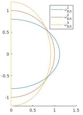
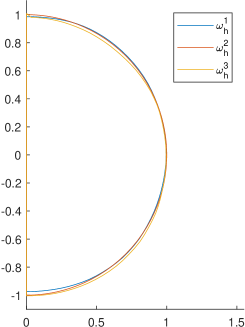
Figure 1: Initial domains $\omega_{0,h}^{i}$ and resulting optimal domains $\omega_{h}^{i}$, $i=1,2,3$ of (6.1), approximately a ball, with constraint $|\omega|_{r}=2/3$

6.2 Eigenvalue Arising in a Problem of Optimal Insulation

The reduced variant of the problem of optimal insulation led to the following two-dimensional discrete problem.

Minimize $$\lambda^{r,\varepsilon,h}_{m}(\omega_{h})$$

w.r.t. $$\omega_{h}\subset\mathbb{R}_{+}\times\mathbb{R},\ \mathcal{T}_{h}\in\mathbb{T}_{c_{\textup{usr}}}\textup{ triangulation of }\omega_{h} \mathbf{P_{m,h,\varepsilon}}$$ ()

s.t. $$u_{h}\in\mathcal{S}^{1}(\mathcal{T}_{h})\textup{ solves }\eqref{eq:reg_var_dis}\textup{ and }\|u_{h}\|_{L^{2}_{r}(Q)}=1$$

$$\omega_{h}\subset Q\textup{ is convex and open and }2\pi|\omega_{h}|_{r}=M$$

and $$\text{the rotated domain }R(\omega_{h})\subset\mathbb{R}^{3}\text{ is also convex}$$

for the class $\mathbb{T}_{c_{\textup{usr}}}$ of conforming, uniformly shape regular triangulations $\mathcal{T}_{h}$ of polyhedral subsets of $\mathbb{R}^{2}$ with $h_{T}/\varrho_{T}\leq c_{\textup{usr}}$ for all elements $T\in\mathcal{T}_{h}$ with diameter $h_{T}\leq h$ and inner radius $\varrho_{T}$ for a universal constant $c_{\textup{usr}}>0$.

We look at several values for the mass $m$. From [16] we know, that for the ball symmetry breaking for the distribution of insulating material occurs if $m$ is below a critical value.

Theorem 1 (c.f. [16], Theorem 3.1)

Let $\Omega$ be a ball. Then there exists $m_{0}>0$ such that the eigenfunction to (7) is radial if $m>m_{0}$, while the solution is not radial for $0<m<m_{0}$. As a consequence, the optimal insulation thickness $\ell_{opt}$ is not constant if $m<m_{0}$.

In [16] it is further noted, that this threshold is given by the unique positive $m$ for which $\lambda_{m}=\mu_{2}$, the first non-zero eigenvalue of the Neumann problem. Furthermore it is proven, that for $m<m_{0}$ the ball is not a stationary domain for the shape optimization problem. We can use the Neumann eigenvalue to approximate the value for the threshold $m_{0}$ of the dimensionally reduced problem for the ball, which is given by approximately $m_{0}\approx 5.7963$.

We next address numerical approximations for the values $m=2,5,6,11,12$ and $13$. The experimental results displayed in Tables 4 and 5 and Figures 2, 3 and 4 were obtained on triangulations $\mathcal{T}_{h}$ with maximal mesh size $h=2^{-5}$ and regularization parameter $\varepsilon=N^{-1/2}/10$, where $N$ is the number of nodes of $\mathcal{T}_{h}$. The numerical experiments confirm that for the two values lower then the critical mass, the ball is no stationary domain. Only one asymmetric optimal domain was found for each value of $m$, c.f. Figure 2 and Table 4. For the larger values, in the numerical experiments the ball is also stationary, and for $m=11,12$ and $13$ it is experimentally optimal, see Figures 4 and Tables 5. As in Section 6.1 half-ellipsoids with different ratios were chosen as initial domains. For values of $m$ where more than one stationary domain was approximated, the result of the optimization algorithm depended on the choice of the ratios for the initial domains. In general, depending on the value $m$, when initial domains were chosen that are more prolate, an asymmetric domain was approximated, while oblate ellipsoids and ellipsoids closer to the ball led to the ball being approximated.

The algorithm only detects local minima with the approximated domains depending on the initial domains, so the stationary domains approximated might not be global solutions.
When comparing the approximated optimal domains with each other, we also observe that for the non-radial solutions, a large portion of the insulating film concentrates in one area, which creates a hotspot inside the domain, where the temperature is preserved better, while other areas are neglected, having no insulating material on the boundary.

Remark 2

We briefly note, that even though we search for eigenfunctions among rotationally symmetric functions, the numerical results are still consistent with the expectations we have from [16] regarding the radial symmetry for the eigenfunctions for the ball. We were able to observe that for $m<m_{0}$, the critical value related to the Neumann eigenvalue, c.f. Theorem 1, the eigenfunction is no longer positive or symmetric, c.f. Figure 3, but for values $m>m_{0}$ it is. Further, the shape optimization problem showed, that for the chosen values $m<m_{0}$ the ball was no stationary domain, while for $m>m_{0}$ it was stationary and for the higher values even optimal. This consistency of the numerical results suggests, that the restriction to rotationally symmetric functions is justified.
The critical value $m_{0}$ relates to the symmetry of the eigenfunctions on the ball and whether the ball is a stationary domain. Theorem 3.1 in [16] does not consider the optimality of the ball under the shape optimization. However, the experimental results of the shape optimization suggest that there might be another critical value of mass $m_{1}$, such that for $m<m_{1}$ an asymmetric domain yields an optimal eigenvalue, while for $m>m_{1}$ the ball is the optimal domain.

We want to take a closer look at the properties of the optimal domains for the eigenvalue problem in optimal insulation. First we will look at the improvement of the eigenvalue the shape optimization provides and afterward at the optimal domains themselves. The experiments in this section were obtained with a triangulation with a maximal mesh size $h=2^{-4}$ and $\varepsilon$ chosen as in the previous experiments.

Comparing the eigenvalue of the ball to that of the respective stationary asymmetric domain for different values of mass $m$, c.f. Figure 5, shows that the benefit of the shape optimization is greatest around the critical value $m_{0}$.

Next, we take a closer look at the optimal domains. For the masses $m=1,2,..,12$ the optimal domains with insulating film are displayed in Figure 6. As $m$ decreases, the eigenvalue is closer to the eigenvalue of the Dirichlet Laplacian. We notice, for $m=1$, the approximated optimal shape is closer to a ball, and as the values $m$ increase the optimal domains become more prolate, until, for $m=12$, the ball is the approximated optimal domain.

We further notice that for the asymmetric domains a kink is formed around the surface area where the eigenfunction is zero. For $m=2,...,9$, this kink might even be non-smooth. By taking a closer look at the values of the eigenfunction at the boundary nodes and the mean curvature of the boundary $\Gamma_{\textup{out}}$ for the approximated optimal domains, c.f. Figure 7, we can see that this kink is located around the surface, where no insulating material is placed, and that for the values where the kink might be non-smooth, it is located where the eigenfunction vanishes. The insulating material then focuses on one side of the kink. The corresponding domains are those shown in Figure 6. In summary, the numerical experiments suggest, that the asymmetric optimal domains tend to be non-smooth for lower values of $m$.

Acknowledgments: This work is supported by DFG grants BA2268/4-2 within the Priority Program SPP 1962 (Non- smooth and Complementarity-based Distributed Parameter Systems: Simulation and Hierarchical Optimization).

	$\lambda^{r,\varepsilon}(\omega_{h})$	$|\omega_{h}|_{r}$
$m=2$	6.819940118007397	0.6595
$m=5$	4.554732496286795	0.6596

Table 4: Eigenvalues $\lambda^{r,\varepsilon}_{m}$ of approximated optimal domains for different values of $m<m_{0}$ c.f. Figure 2, with constraint $|\omega|_{r}=2/3$

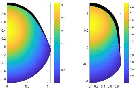
Figure 2: Optimal domains $\omega_{h}$ of (6.2) for $m=2$ (left), $m=5$ (right), with boundary film (black, scaled with $\epsilon=1/10$) and eigenfunction (shaded), with constraint $|\omega|_{r}=2/3$; corresponding eigenvalues c.f. Table 4

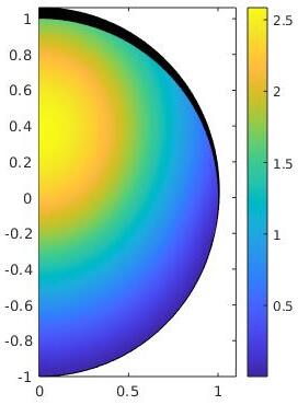
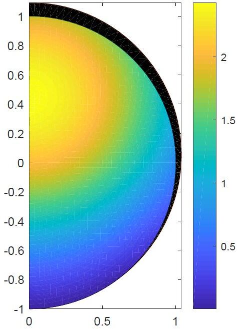
Figure 3: Non-radial eigenfunctions (shaded) with boundary film (black, scaled with $\epsilon=1/10$) for $m=2$ (left) and $m=5$ (right) for the fixed ball

	$\lambda^{r,\varepsilon}_{m}(\omega^{1}_{h})$	$|\omega^{1}_{h}|_{r}$	$\lambda^{r,\varepsilon}_{m}(\omega^{2}_{h})$	$|\omega^{2}_{h}|_{r}$
$m=6$	4.112232986601394	0.6631	4.241084607303154	0.6662
$m=11$	2.769366507533780	0.6633	2.744289963928029	0.6662
$m=12$	2.606239519805330	0.6621	2.561023079370016	0.6662
$m=13$	2.459976343090586	0.6633	2.400341990779929	0.6662

Table 5: Eigenvalues $\lambda^{r,\varepsilon}_{m}$ of approximated stationary domains $\omega^{1}_{h}$ (asymetric) and $\omega_{h}^{2}$ (half-disk), c.f. Figure 4 for different values of $m$, with constraint $|\omega|_{r}=2/3$

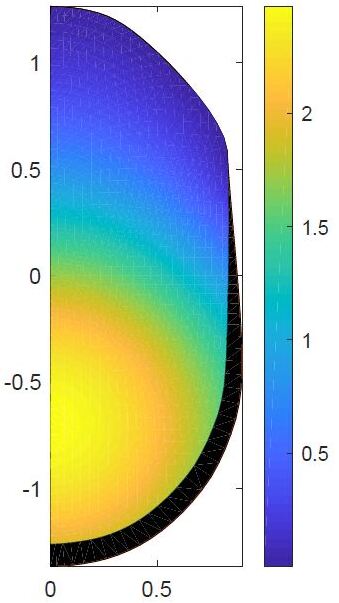
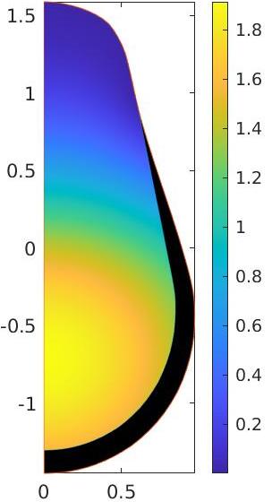
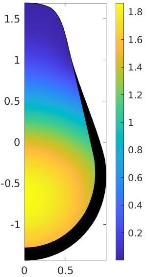
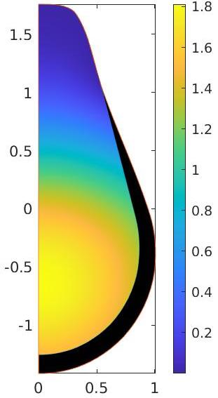
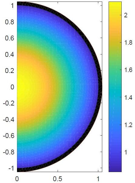
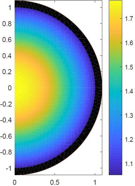
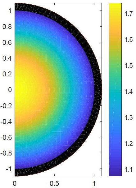
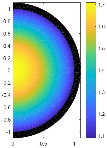
Figure 4: Approximated stationary domains $\omega^{i}_{h}$ ($i=1$ top, $i=2$ bottom) of (6.2) for $m=6,11,12$ and $13$ (left to right), with boundary film (black, scaled with $\epsilon=1/10$) and eigenfunction (shaded), with constraint $|\omega|_{r}=2/3$; corresponding eigenvalues c.f. Table 5black. For $m=6,11$ the asymmetric domains (top) are optimal, for $m=12,13$ the half-disk (bottom) is optimal. The other domains are stationary but not optimal under the shape optimization.

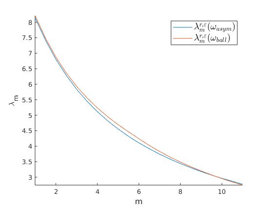
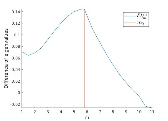
Figure 5: Eigenvalues of the asymmetric stationary domain and the ball compared for different values of $m$ (left) and difference in eigenvalues $\delta\lambda_{m}^{r,\varepsilon}=\lambda_{m}^{r,\varepsilon}(\omega_{\text{ball}})-\lambda_{m}^{r,\varepsilon}(\omega_{\text{asym}})$ with peak at the critical value $m_{0}$ (right)

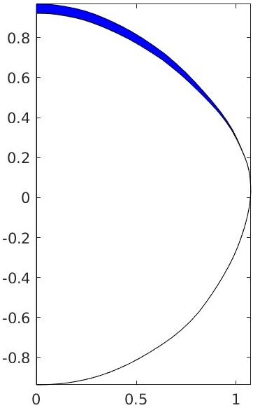
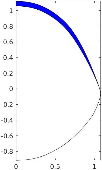
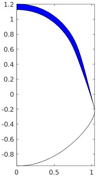
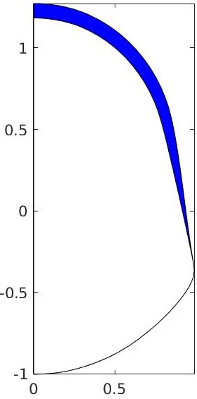
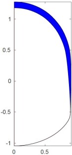
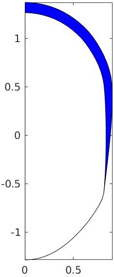
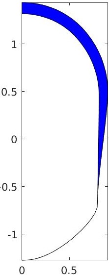
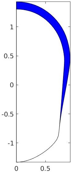
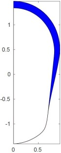
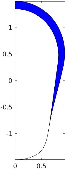
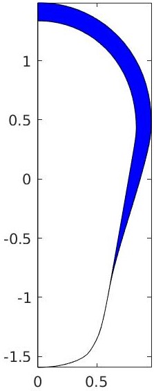
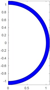
Figure 6: Approximated stationary and optimal domains for $\lambda^{r,\varepsilon}_{m}$ for $m=1$ to $12$ (left to right, top to bottom) and insulating film (blue, scaled with $\epsilon=1/10$)

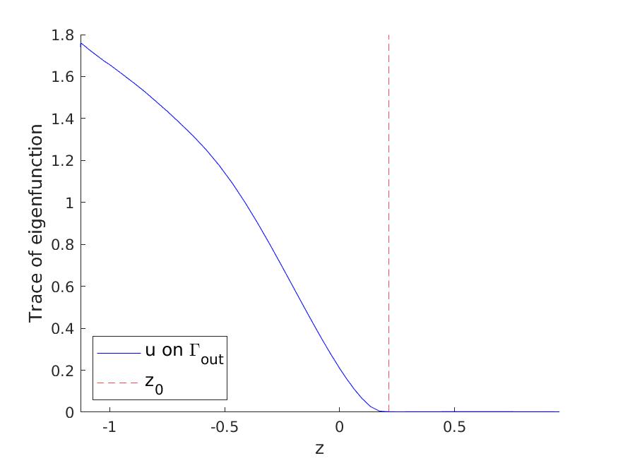
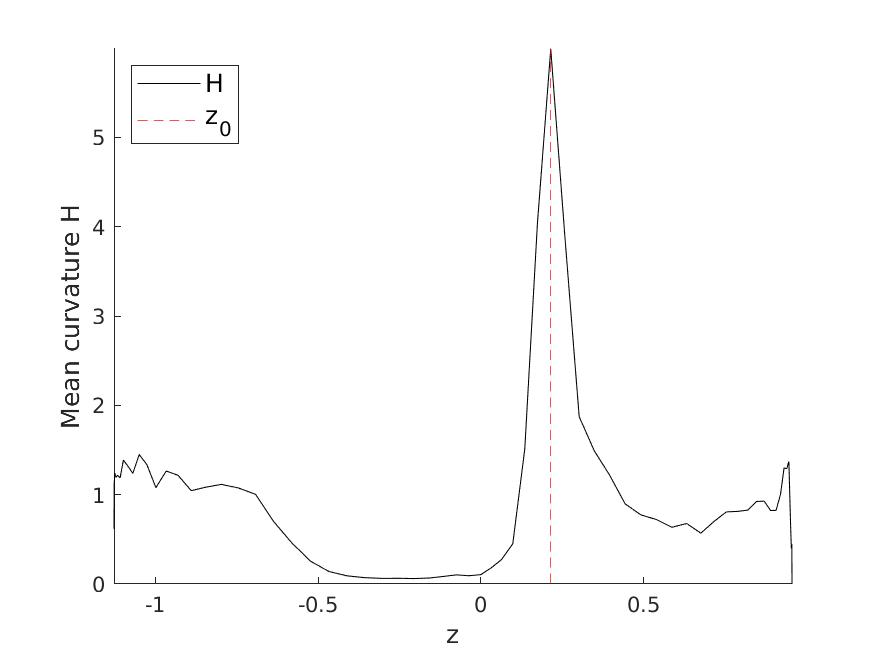
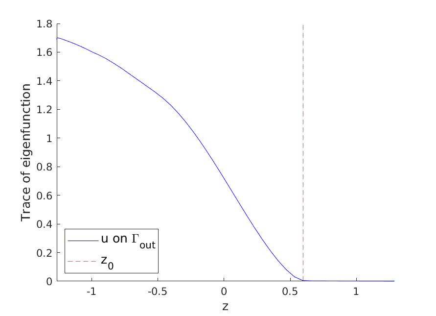
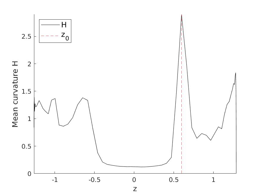
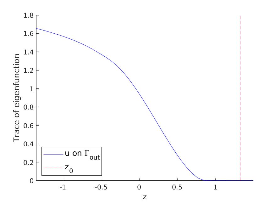
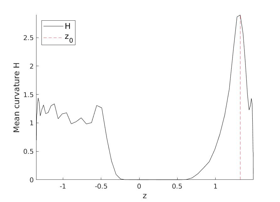
Figure 7: Values of eigenfunctions (left) and mean curvature (right) along the boundary curve (as a function of $z$ along the axis of rotation) of optimal domains for $m=3,6$, and $10$ (top to bottom), with approximate location $z_{0}$ of the kink in the boundary on a triangulation with maximal mesh size $h=2^{-4}$. The corresponding domains are shown in Figure 6.

References

• [1]
• Aguilera and Morin [2009] Néstor E Aguilera and Pedro Morin. On convex functions and the finite element method. SIAM Journal on Numerical Analysis, 47(4):3139–3157, 2009. doi:10.1137/080720917.
• Antil et al. [2018] Harbir Antil, Enrique Otárola, and Abner J Salgado. Some applications of weighted norm inequalities to the error analysis of pde-constrained optimization problems. IMA Journal of Numerical Analysis, 38(2):852–883, 2018. doi:10.1093/imanum/drx018.
• Antunes and Bogosel [2018] Pedro RS Antunes and Beniamin Bogosel. Parametric shape optimization using the support function. arXiv preprint arXiv:1809.00254, 2018. URL https://arxiv.org/abs/1809.00254.
• Atamni et al. [2001] H. Atamni, M. El Hatri, and N. Popivanov. Polynomial approximation in weighted Sobolev space. C. R. Acad. Bulgare Sci., 54(3):25–30, 2001. ISSN 1310-1331. URL adsabs.harvard.edu/pdf/2001CRABS..54c..25A.
• Attouch et al. [2014] Hedy Attouch, Giuseppe Buttazzo, and Gérard Michaille. Variational analysis in Sobolev and BV spaces: applications to PDEs and optimization. SIAM, 2014. doi:10.1137/1.9781611973488.
• Bartels [2016] Sören Bartels. Numerical approximation of partial differential equations, volume 64. Springer, 2016. doi:10.1007/978-3-319-32354-1.
• Bartels and Buttazzo [2019] Sören Bartels and Giuseppe Buttazzo. Numerical solution of a nonlinear eigenvalue problem arising in optimal insulation. Interfaces Free Bound., 21(1):1–19, 2019. doi:10.4171/IFB/414.
• Bartels and Wachsmuth [2020] Sören Bartels and Gerd Wachsmuth. Numerical approximation of optimal convex shapes. SIAM Journal on Scientific Computing, 42(2):A1226–A1244, 2020. doi:10.1137/19M1256853.
• Boffi et al. [2013] Daniele Boffi, Franco Brezzi, and Michel Fortin. Mixed finite element methods and applications, volume 44 of Springer Series in Computational Mathematics. Springer, Heidelberg, 2013. ISBN 978-3-642-36518-8; 978-3-642-36519-5. doi:10.1007/978-3-642-36519-5.
• Braess [2013] Dietrich Braess. Finite Elemente: Theorie, schnelle Löser und Anwendungen in der Elastizitätstheorie. Springer-Verlag, 2013. doi:10.1007/978-3-642-34797-9.
• Bucur [2003] Dorin Bucur. Regularity of optimal convex shapes. Journal of Convex Analysis, 10(2):501–516, 2003. URL https://www.heldermann-verlag.de/jca/jca10/jca0397.pdf.
• Bucur and Buttazzo [2004] Dorin Bucur and Giuseppe Buttazzo. Variational methods in shape optimization problems, volume 65. Springer-Progress in Nonlinear Differential Equations and Their Applications, 2004. doi:10.1007/b137163.
• Bucur and Giacomini [2010] Dorin Bucur and Alessandro Giacomini. A variational approach to the isoperimetric inequality for the Robin eigenvalue problem. Arch. Ration. Mech. Anal., 198(3):927–961, 2010. doi:10.1007/s00205-010-0298-6.
• Bucur and Giacomini [2016] Dorin Bucur and Alessandro Giacomini. Shape optimization problems with Robin conditions on the free boundary. Ann. Inst. H. Poincaré Anal. Non Linéaire, 33(6):1539–1568, 2016. doi:10.1016/j.anihpc.2015.07.001.
• Bucur et al. [2017] Dorin Bucur, Giuseppe Buttazzo, and Carlo Nitsch. Symmetry breaking for a problem in optimal insulation. Journal de Mathématiques Pures et Appliquées, 107(4):451–463, 2017. doi:10.1016/j.matpur.2016.07.006.
• Buttazzo and Guasoni [1997] Giuseppe Buttazzo and Paolo Guasoni. Shape optimization problems over classes of convex domains. J. Convex Anal., 4(2):343–351, 1997. URL https://www.guasoni.com/papers/resmin.pdf.
• Choné and Le Meur [2001] Philippe Choné and Hervé V. J. Le Meur. Non-convergence result for conformal approximation of variational problems subject to a convexity constraint. Numer. Funct. Anal. Optim., 22(5-6):529–547, 2001. doi:10.1081/NFA-100105306.
• Eggleston [1958] H. G. Eggleston. Convexity. Cambridge Tracts in Mathematics. Cambridge University Press, 1958. doi:10.1017/CBO9780511566172.
• El Hatri [1987] Mohamed El Hatri. Estimation d’erreur optimale et de type superconvergence de la méthode des éléments finis pour un problème aux limites, dégénéré. RAIRO Modél. Math. Anal. Numér., 21(1):27–61, 1987. ISSN 0764-583X. doi:10.1051/m2an/1987210100271.
• Glowinski et al. [1981] Roland Glowinski, Jacques-Louis Lions, and Raymond Trémolières. Numerical analysis of variational inequalities, volume 8 of Studies in Mathematics and its Applications. North-Holland Publishing Co., Amsterdam-New York, 1981. ISBN 0-444-86199-8. URL https://www.sciencedirect.com/bookseries/studies-in-mathematics-and-its-applications/vol/8/suppl/C. Translated from the French.
• Henrot [2017] Antoine Henrot. Shape optimization and spectral theory. De Gruyter, 2017. doi:10.1515/9783110550887.
• Henrot and Pierre [2006] Antoine Henrot and Michel Pierre. Variation et optimisation de formes: une analyse géométrique, volume 48. Springer Science & Business Media, 2006. doi:10.1007/3-540-37689-5.
• Hinze et al. [2009] M. Hinze, R. Pinnau, M. Ulbrich, and S. Ulbrich. Optimization with PDE constraints, volume 23 of Mathematical Modelling: Theory and Applications. Springer, New York, 2009. ISBN 978-1-4020-8838-4. URL https://link.springer.com/book/10.1007/978-1-4020-8839-1.
• Krahn [1925] Edgar Krahn. Über eine von Rayleigh formulierte Minimaleigenschaft des Kreises. Mathematische Annalen, 94(1):97–100, 1925. doi:10.1007/BF01208645.
• Krahn [1926] Edgar Krahn. Über Minimaleigenschaften der Kugel in drei und mehr Dimensionen. Mattiesen, 1926.
• Lachand-Robert and Oudet [2005] Thomas Lachand-Robert and Édouard Oudet. Minimizing within convex bodies using a convex hull method. SIAM Journal on Optimization, 16(2):368–379, 2005. doi:10.1137/040608039.
• Nochetto et al. [2016] Ricardo H. Nochetto, Enrique Otárola, and Abner J. Salgado. Piecewise polynomial interpolation in Muckenhoupt weighted Sobolev spaces and applications. Numer. Math., 132(1):85–130, 2016. ISSN 0029-599X. doi:10.1007/s00211-015-0709-6.
• Payne and Weinberger [1960] Lawrence E Payne and Hans F Weinberger. An optimal poincaré inequality for convex domains. Archive for Rational Mechanics and Analysis, 5(1):286–292, 1960. doi:10.1007/BF00252910.
• Sokoł owski and Zolésio [1992] Jan Sokoł owski and Jean-Paul Zolésio. Introduction to shape optimization, volume 16 of Springer Series in Computational Mathematics. Springer-Verlag, Berlin, 1992. ISBN 3-540-54177-2. doi:10.1007/978-3-642-58106-9. URL https://doi.org/10.1007/978-3-642-58106-9. Shape sensitivity analysis.
• Steinhagen [1922] Paul Steinhagen. Über die größte Kugel in einer konvexen Punktmenge. Abh. Math. Sem. Univ. Hamburg, 1(1):15–26, 1922. ISSN 0025-5858. doi:10.1007/BF02940577.
• Van Goethem [2004] Nicolas Van Goethem. Variational problems on classes of convex domains. Communications in Applied Analysis 8.3, pages 353–371, 2004. URL https://arxiv.org/abs/math/0703734.
• Wachsmuth [2017] Gerd Wachsmuth. Conforming approximation of convex functions with the finite element method. Numerische Mathematik, 137(3):741–772, 2017. doi:10.1007/s00211-017-0884-8.
• Yang [2009] Donghui Yang. Shape optimization of stationary navier–stokes equation over classes of convex domains. Nonlinear Analysis: Theory, Methods & Applications, 71(12):6202–6211, 2009. doi:10.1016/j.na.2009.06.013.