Global analysis of a spatiotemporal cellular model for the transmission of hepatitis C virus with Hattaf-Yousfi functional response

Abstract

In this paper, a mathematical analysis of the global dynamics of a partial differential equation viral infection cellular model is carried out. We study the dynamics of a hepatitis C virus (HCV) model, under therapy, that considers both absorption phenomenon and diffusion of virions, infected and uninfected cells in liver. Firstly, we prove boundedness of the potential solutions, global existence, uniqueness and positivity of the solutions to the obtained initial value and boundary problem. Then, the dynamical behavior of the model is completely determined by a threshold parameter called the basic reproduction number $\mathcal{R}_{0}$. We show that the uninfected spatially homogeneous equilibrium of the model is globally asymptotically stable if $\mathcal{R}_{0}\leq 1$ by using the direct Lyapunov method. This means that the HCV is cleared and the disease dies out. Also, the global asymptotically properties stability of the infected spatially homogeneous equilibrium of the model are studied via a skilful construction of a suitable Lyapunov functional. It means that the HCV persists in the host and the infection becomes chronic. Finally, numerical simulations are performed to support the theoretical results obtained.

1 Introduction

The dynamics of viruses, in particular the dynamics of the hepatitis C virus, remains a very active field of research in the world of science. Moreover, the 2020 Nobel Prize in Medicine was awarded to three researchers, namely the British Michael Hougton and the Americans Harvey Alter and Charles Rice. They were awarded this Nobel Prize for their very advanced research work on the hepatitis C virus.

According to World Health Organization(WHO) who1 , 71 million persons were living with chronic hepatitis C virus (HCV) infection worldwide and 399 000 persons had died from cirrhosis or hepatocellular carcinoma following a survey done in 2015. Aside from the burden of HCV infection secondary to liver-related sequelae, HCV causes an additional burden through comorbidities among persons with HCV infection, including depression, diabetes mellitus and chronic renal disease. In May 2016, the World Health Assembly endorsed the Global Health Sector Strategy for 2016-2021 on viral hepatitis (HBV and HCV infection), which proposes to eliminate viral hepatitis as a public health threat by 2030. Elimination is defined as a 90% reduction in new chronic infections and a 65% reduction in mortality compared with the 2015 baseline.

Mathematicians cannot stay aside from disastrous situation decried by WHO. In view of the vital importance of the liver and the aforementioned facts, any contribution to a better understanding of HCV infection process is of great interest. Mathematical models have been developed to help understand and control the dynamics of HCV within an infected host such as in chong2015 ; Rongetal2013 ; chatterjeeetal2012 ; Guedjetneumann2010 . The dynamics of viral infections such as the Ebola virus disease(EVD), the human immunodeficiency virus (HIV) infection, the hepatitis B virus (HBV) infection, the hepatitis C virus (HCV) infection and, new corona virus infection have been modeled mathematically in a host. One of the earliest temporal models was the within-host basic viral infection model proposed in nowakbagham to study HIV infection, and later adopted to HBV nowakbonofer ; ciupeetal2007 . Particularly, numerous mathematical models describing the temporal dynamics of HCV have been initially proposed by Neumann and al neumanetal1998 using the classical viral infection cellular model, and later have been extended in Daharietal2007 ; Guedjetneumann2010 ; chatterjeeetal2012 ; Rongetal2013 . Motivated by what has been done in nowakbonofer ; ciupeetal2007 ; neumanetal1998 , Chong and al.chong2015 formulated the basic HCV temporal intra-host model or cellular model infection with therapy as a system of three differential equations :

$$\frac{dH(t)}{dt}=\lambda-dH(t)-(1-\eta)\beta H(t)V(t),$$

$$\frac{dI(t)}{dt}=(1-\eta)\beta H(t)V(t)-\alpha I(t),$$ (1)

$$\frac{dV(t)}{dt}=(1-\varepsilon)kI(t)-\mu V(t),$$

where the equations relate the dynamics relationship between, H as the uninfected target cells (hepatocytes), I as the infected cells and V as the viral load (amount of viruses present in the blood). In the system (1) the key assumption is that hepatocytes and viruses are well mixed, and ignores the mobility of hepatocytes C viruses, the infected and uninfected target cells. To study the influences of spatial structures of virus dynamics, Wang and Wang in wangwang assuming that the motion of virus follows Fickian diffusion, that is to say, the population flux of virus is proportional to the concentration gradient and the proportionality constant is taken to be negative fichian .
Moreover, in system (1), the rate of infection is assumed to be bilinear in the virus V and uninfected hepatocytes T. It is shown in minetal that this bilinear rate of infection could be unrealistic. However, the actual incidence rate is probably not linear over the entire range of T and V. Thus is reasonable to assume that the infection rate is given by a more general one, known as the Hattaf-Yousfi functionnal response HattafK2016 of the form $\frac{\beta HV}{\alpha_{0}+\alpha_{1}H+\alpha_{2}V+\alpha_{3}HV}$ where $\alpha_{0}>0$, $\alpha_{1}\geq 0$, $\alpha_{2}\geq 0$, $\alpha_{3}\geq 0$ are constants. The function $\frac{\beta H}{\alpha_{0}+\alpha_{1}H+\alpha_{2}V+\alpha_{3}HV}$ satisfies the hypotheses $(H_{1})$, $(H_{2})$ and $(H_{3})$ of general incidence rate presented in Hattafetal2012 ; Hattafetal2013a ; Hattafetal2013b ; HY1 . The Hattaf-Yousfi type of functional response was introduced by Hattaf and al. in HattafK2016 . This functional response generalizes many functional responses and it was used in riad2016 to describe the dynamics of labour market. Thus, when $\alpha_{0}=1$, the Hattaf-Yousfi functional response is reduced to the specific functional response used by Hattaf and al in Hattafetal2015 . Furthermore, if $\alpha_{3}=\alpha_{1}\alpha_{2}$ and $\alpha_{0}=1$, the Hattaf-Yousfi functional response is reduced to Crowley-Martin functional response crowleym1989 and was used in zhouandcui2011 . When $\alpha_{3}=0$ et $\alpha_{0}=1$ the Hattaf-Yousfi functional response is simplified to Beddington-DeAngelis functional responseBedding1975 ; Deangelisetal1975 , and was used in huang2009 ; huang2011 ; wangetal2011 ; zhangxu2013 . When $\alpha_{1}>0$, $\alpha_{2}=\alpha_{3}=0$ and $\alpha_{0}=1$, the Hattaf-Yousfi functional response is reduced to Holling type II functional responseLiandma2007 . And when $\alpha_{1}=\alpha_{3}=0$, $\alpha_{2}>0$ and $\alpha_{0}=1$ it expresses a saturation responseSongneuman2007 . Moreover, when $\alpha_{1}=\alpha_{2}=\alpha_{3}=0$, and $\alpha_{0}=1$ the Hattaf-Yousfi functional response is reduced to the mass action principle(or Holling type I functional response). Also ordinary differential system (1)take into consideration the cure of infected hepatocytes.
In this work, motivated by the breaches observed in the analysis and the formulation of system (1), we construct and analyze a PDE-cellular model system for HCV infection, which derives from system (1) by incorporating the space, Hattaf-Yousfi incidence rate, absorption effect and spontaneous cure. It is worth mentioning that in chong2015 the authors used mass-action kinetics for viral infection, neglected the cure rate, ignored the absorption effect and the diffusion of free virions, susceptible cells and infected cells. So the obtained model is an extension of the one in the first of work done by Chong and al.chong2015 .
The work is organized as follows. In section 2, we model the phenomenon described through a system of partial differential equations which leads to a initial value and boundary problem. Section 3 is devoted to the study of the existence and uniqueness of the global solution of our initial and boundary value problem, and of the properties of this solution, namely positivity and boundedness. Section 4 deals with the stability and the analysis of spatially homogeneous equilibria and numerical simulations in section 5. We conclude our work and provide a discussion in section 6.

2 Formulation of the PDE-cellular model

Let $\Omega\subset\mathds{R}^{3}$ be the domain representing the liver. Let $t\geq 0$ be a given time and $x=(x_{1},x_{2},x_{3})\in\Omega$. Denote respectively by $H(x,t)$, $I(x,t)$ and $V(x,t)$ the concentrations of healthy hepatocytes, HCV infected hepatocytes, and free HCV virions at time $t$ and location $x$. The dynamics of HCV infection intra-host is the result of the dynamics of each compartment H, I, and V, and the various interactions between them. We now describe the evolution of each compartment.

Fluctuation of healthy hepatocytes.

Let $\nu$ be an elementary volume in $\Omega$. The variation of the quantity of healthy hepatocytes in $\nu$ is described under the following assumptions. Healthy hepatocytes are produced at constant rate $\lambda$ from the bone marrow and die at rate $dH$. Virions infect the healthy hepatocytes at the rate $\frac{\beta HV}{\alpha_{0}+\alpha_{1}H+\alpha_{2}V+\alpha_{3}HV},$ where $\beta$ is the rate of transmission of the infection and $\alpha_{j}$, $j=0,1,2,3$ are positive constants. This generalized incidence function replaces the mass-action function which has been shown to cause unrealistic conditions for successful chronic HCV infection. $\rho I$ is the cure rate of infected hepatocytes either by noncytolytic mechanism or immunity or treatment. In addition, the therapeutic effect of treatment in this model involved the reduction of new infections, which is described in a fraction as $(1-\eta)$. The spatial motion of healthy hepatocytes follows the Fickian diffusion law. Thus, the variation of healthy hepatocytes is expressed by the following equation:

$$\frac{\partial H}{\partial t} = D_{1}\Delta H(x,t)+\lambda-dH(x,t)$$

$$-\frac{(1-\eta)\beta H(x,t)V(x,t)}{\alpha_{0}+\alpha_{1}H(x,t)+\alpha_{2}V(x,t)+\alpha_{3}H(x,t)V(x,t)}+\rho I(x,t),$$

where $D_{1}$ represents the Healthy hepatocytes diffusion coefficient and

$$\Delta=\frac{\partial^{2}}{\partial x_{1}^{2}}+\frac{\partial^{2}}{\partial x_{2}^{2}}+\frac{\partial^{2}}{\partial x_{3}^{2}}$$

is the usual Laplacian operator in three-dimensional space.

Fluctuation of HCV infected cells.

The HCV infected cells die at rate $\alpha$ per day so that $\frac{1}{\alpha}$ is the life-expectancy of HCV infected hepatocytes. Healthy hepatocytes become infected at the rate $\frac{\beta HV}{\alpha_{0}+\alpha_{1}H+\alpha_{2}V+\alpha_{3}HV}$. The spatial motion of HCV infected cells follows the Fickian diffusion law. Thus, the variation of infected hepatocytes is expressed by the following equation

$$\frac{\partial I}{\partial t}=D_{2}\Delta I(x,t)+\frac{(1-\eta)\beta H(x,t)V(x,t)}{\alpha_{0}+\alpha_{1}H(x,t)+\alpha_{2}V(x,t)+\alpha_{3}H(x,t)V(x,t)}-(\alpha+\rho)I(x,t),$$

where $D_{2}$ represents the HCV infected cells diffusion coefficient.

Fluctuation of free HCV virions.

The infected hepatocytes produce virus at rate $kI$, and virus is cleared at the rate $\mu V$. Also, the population of virions decreases due to the infection at the rate $\frac{u(1-\eta)\beta HV}{\alpha_{0}+\alpha_{1}H+\alpha_{2}V+\alpha_{3}HV}$ due to absorption effect, where $u\in¸\{0,1\}$. The spatial motion of virions follows the Fickian diffusion law. In addition, the therapeutic effect of treatment in this model involved blocking virions production (referred to as drug effectiveness) which, is described in fraction $(1-\varepsilon)$. Thus, the variation of free virions is expressed by the following equation:

$$\frac{\partial V}{\partial t} = D_{3}\Delta V(x,t)+(1-\varepsilon)kI(x,t)-\mu V(x,t)$$

$$-u\frac{(1-\eta)\beta H(x,t)V(x,t)}{\alpha_{0}+\alpha_{1}H(x,t)+\alpha_{2}V(x,t)+\alpha_{3}H(x,t)V(x,t)},$$

where $D_{3}$ represents the free HCV virions diffusion coefficient.

The initial boundary value problem associated to PDE-cellular model.

In this section, we use the previous equations describing variables variations to set up a complete PDE system modeling biological dynamics for HCV infection. Let $T>0$ be a fixed time and define

$$\Omega_{T}=\Omega\times(0,T).$$

Therefore, in $\Omega_{T}$ the full system of PDE governing the HCV infection becomes :

$$\frac{\partial H}{\partial t}=D_{1}\Delta H(x,t)+\lambda-dH-\frac{(1-\eta)\beta HV}{\alpha_{0}+\alpha_{1}H+\alpha_{2}V+\alpha_{3}HV}+\rho I,$$

$$\frac{\partial I}{\partial t}=D_{2}\Delta I(x,t)+\frac{(1-\eta)\beta HV}{\alpha_{0}+\alpha_{1}H+\alpha_{2}V+\alpha_{3}HV}-(\alpha+\rho)I,$$ (2)

$$\frac{\partial V}{\partial t}=D_{3}\Delta V+(1-\varepsilon)kI-\mu V-\frac{u(1-\eta)\beta HV}{\alpha_{0}+\alpha_{1}H+\alpha_{2}V+\alpha_{3}HV}.$$

We use the Neumann homogeneous boundary conditions:

$$\frac{\partial H}{\partial\eta}=\frac{\partial I}{\partial\eta}=\frac{\partial V}{\partial\eta}=0\;\;\mbox{on}\;\partial\Omega\times[0,T],$$ (3)

where $\frac{\partial}{\partial\eta}$ denotes the outward normal derivative on $\partial\Omega$. The initial conditions are the following :

$$H(x,0)=H_{0},\;\;I(x,0)=I_{0},\;\;V(x,0)=V_{0},\;\;x\in\Omega.$$ (4)

The boundary conditions in (3) imply that the Healthy hepatocytes, the HCV infected cells and free HCV virions do not move across the boundary $\partial\Omega$. For an epidemiological significance, we assume that the initial conditions are positive and Hölder continuous, and satisfy $\frac{\partial H_{0}}{\partial\eta}=\frac{\partial I_{0}}{\partial\eta}=\frac{\partial V_{0}}{\partial\eta}=0$ on $\partial\Omega$.
We then obtain the following initial boundary value problem (IBVP) associated to our PDE-cellular model:

$$\frac{\partial H}{\partial t}=D_{1}\Delta H+\lambda-dH-\frac{(1-\eta)\beta HV}{\alpha_{0}+\alpha_{1}H+\alpha_{2}V+\alpha_{3}HV}+\rho I\;\;\mbox{in}\;\;\Omega_{T},$$

$$\frac{\partial I}{\partial t}=D_{2}\Delta I+\frac{(1-\eta)\beta HV}{\alpha_{0}+\alpha_{1}H+\alpha_{2}V+\alpha_{3}HV}-(\alpha+\rho)I\;\;\mbox{in}\;\;\Omega_{T},$$

$$\frac{\partial V}{\partial t}=D_{3}\Delta V+(1-\varepsilon)kI-\mu V-\frac{u(1-\eta)\beta HV}{\alpha_{0}+\alpha_{1}H+\alpha_{2}V+\alpha_{3}HV}\;\;\mbox{in}\;\;\Omega_{T},\;\;$$ (5)

$$\frac{\partial H}{\partial\eta}=\frac{\partial I}{\partial\eta}=\frac{\partial V}{\partial\eta}=0\;\;\mbox{on}\;\;\partial\Omega\times[0,T],$$

$$H(x,0)=H_{0},\;I(x,0)=I_{0},\;V(x,0)=V_{0},\;\;x\in\Omega,$$

on which our study will focus on.

3 Quantitative analysis and some properties of the solutions for IBVP (5)

In this section, we provide a thorough study of the dynamics of IBVP (5) which yields various outcomes. Precisely, we prove existence, uniqueness, positivity and boundedness of solutions for IBVP (5). This is done by combining variational method and semigroups techniques to some useful functional analysis arguments.

3.1 Local existence and uniqueness of solutions for the IBVP (5)

Set

$$F(H,I,V)=(F_{1}(H,I,V),F_{2}(H,I,V),F_{3}(H,I,V))^{T}$$ (6)

where

$$F_{1}(H,I,V)=\lambda-dH-\frac{(1-\eta)\beta HV}{\alpha_{0}+\alpha_{1}H+\alpha_{2}V+\alpha_{3}HV}+\rho I,$$

$$F_{2}(H,I,V)=\frac{(1-\eta)\beta HV}{\alpha_{0}+\alpha_{1}H+\alpha_{2}V+\alpha_{3}HV}-(\alpha+\rho)I,$$

and

$$F_{3}(H,I,V)=(1-\varepsilon)kI-\mu V-u\frac{(1-\eta)\beta HV}{\alpha_{0}+\alpha_{1}H+\alpha_{2}V+\alpha_{3}HV}.$$

We have the following result which guarantees that the right-hand side, without diffusion, of the PDE-model system (5) is Lipschitz.

Proposition 1

Let $T\in\mathds{R}_{+}^{*}$ and $(H,I,V)\in(C_{B}^{0}(\Omega\times[0,T]))^{3}$, where $C_{B}^{0}(\Omega\times[0,T])$ is the space of bounded and continuous functions on $\Omega\times[0,T]$. We suppose that F in (6) is defined on $L^{2}(\Omega\times(0,T))$. Then $F_{1},F_{2}$ and $F_{3}$ are uniformly Lipschitz continuous on $L^{2}(\Omega\times(0,T))$ with respect to H, I and V.

Proof: Let $T\in\mathbb{R}_{+}^{*}$ and $(H_{1},I_{1},V_{1}),(H_{2},I_{2},V_{2})\in(C_{B}^{0}(\Omega\times[0,T]))^{3}$. First, by direct computation, we have :

$$\|F_{1}(H_{1},I_{1},V_{1})-F_{1}(H_{2},I_{2},V_{2})\|_{2}\leq K_{1}^{1}\|H_{1}-H_{2}\|_{2}+K_{2}^{1}\|I_{1}-I_{2}\|_{2}+K_{3}^{1}\|V_{1}-V_{2}\|_{2},$$ (7)

with

$$K_{1}^{1}=d+(1-\eta)\beta\left(\frac{1}{\alpha_{2}}+\frac{V_{m}}{\alpha_{0}}\right),\;\;K_{2}^{1}=\rho,\;\;\;\;K_{3}^{1}=(1-\eta)\beta\left(\frac{1}{\alpha_{1}}+\frac{H_{m}}{\alpha_{0}}\right),$$ (8)

with $H_{m}$ and $V_{m}$ given below.
Then

$$\|F_{2}(H_{1},I_{1},V_{1})-F_{2}(H_{2},I_{2},V_{2})\|_{2}\leq K_{1}^{2}\|H_{1}-H_{2}\|_{2}+K_{2}^{2}\|I_{1}-I_{2}\|_{2}+K_{3}^{2}\|V_{1}-V_{2}\|_{2},$$ (9)

with

$$K_{1}^{2}=(1-\eta)\beta\left(\frac{1}{\alpha_{2}}+\frac{V_{m}}{\alpha_{0}}\right),\;\;K_{2}^{2}=(\alpha+\rho)\;\;and\;\;K_{3}^{2}=(1-\eta)\beta\left(\frac{1}{\alpha_{1}}+\frac{H_{m}}{\alpha_{0}}\right).$$ (10)

Finally

$$\|F_{3}(H_{1},I_{1},V_{1})-F_{3}(H_{2},I_{2},V_{2})\|_{2}\leq K_{1}^{3}\|H_{1}-H_{2}\|_{2}+K_{2}^{3}\|I_{1}-I_{2}\|_{2}+K_{3}^{3}\|V_{1}-V_{2}\|_{2},$$ (11)

with

$$K_{1}^{3}=u(1-\eta)\beta\left(\frac{1}{\alpha_{2}}+\frac{V_{m}}{\alpha_{0}}\right),\;\;K_{2}^{3}=k(1-\varepsilon),\;\;and\;\;K_{3}^{3}=\mu+u(1-\eta)\beta\left(\frac{1}{\alpha_{1}}+\frac{H_{m}}{\alpha_{0}}\right).$$ (12)

This completes the proof of Proposition 1.   
Now, consider the following IBVP

$$\left\{\begin{array}[]{lcr}\partial_{t}H-D_{1}\Delta H=f(t,H,I,V)&\mbox{in}&\Omega\times(0,T)\\ \partial_{t}I-D_{2}\Delta I=g(t,H,I,V)&\mbox{in}&\Omega\times(0,T)\\ \partial_{t}V-D_{3}\Delta V=h(t,H,I,V)&\mbox{in}&\Omega\times(0,T)\\ \frac{\partial H}{\partial\eta}=0;\;\frac{\partial I}{\partial\eta}=0;\;\frac{\partial V}{\partial\eta}=0&\mbox{on}&\partial\Omega\times[0,T]\\ H=H_{0},I=I_{0},V=V_{0}&\mbox{on}&\Omega\times\{t=0\}.\end{array}\right.$$ (13)

In the following, we will need the following definition and results.

Definition 1

(Sectorial operator, Henri1981 ) Let A be a linear operator in a Banach space X and suppose A is closed and densely defined. If there exist real numbers $a$, $\omega\in(0,\pi)$, $M\geq 1$ such that

$$\rho(A)\supset\Sigma=\left\{\lambda_{0}\in\mathbb{C}\;:\;\omega\leq arg(\lambda_{0}-a)\leq\pi,\lambda_{0}\neq 0\right\}$$ (14)

and

$$\|R_{\lambda_{0}}(A)\|\leq\frac{M}{|\lambda_{0}-a|}\;\;\mbox{for all}\;\;\lambda_{0}\in\Sigma,$$ (15)

then we say that A is sectorial.

Remark 1

The Neumann realization of the Laplacian $A=-\Delta$, with domain

$$D(A)=\Big{\{}\omega\in H^{2}(\Omega):\frac{\partial\omega}{\partial\eta}=0\Big{\}}$$

is a sectorial operator in $L^{2}(\Omega)$. But since $C_{0}^{\infty}(\Omega)\subset D(A)$, it is densely defined in $L^{2}(\Omega)$. For $\beta\geq 0$ large enough, we define the fractional powers of the Helmholtz operator, $\mathcal{H^{\beta}}=-\Delta+\beta I$, with domain $D(\mathcal{H^{\beta}})$ equipped with graph norm $\|\,.\,\|_{D(\mathcal{H^{\beta}})}=\|\,.\,\|_{2}+\|\mathcal{H^{\beta}}.\|_{2}$.

We have the following general results.

Lemma 1

Adams1975 Let $1\leq p<\infty$. Then $D(\mathcal{H^{\beta}})\subset C_{0}^{\infty}(\Omega)$ with continuous injection for $\beta>\frac{n}{2p}$.

Lemma 2

Henri1981 $D(\mathcal{H}^{\beta})\subset C_{B}^{0}(\Omega)$ with continuous injection for $\beta>\frac{n}{4}$.

Theorem 3.1

Henri1981 If A is sectorial, then $-A$ is the infinitesimal generator of an analytic semigroup, $G(t)$.
If $R_{\lambda_{0}}>a,\;a\in\mathds{R}$ whenever $\lambda_{0}\in\sigma$, then for any $t>0$,

$$\|G(t)\|\leq Ce^{-at}\;,\;\;\;\|AG(t)\|\leq\frac{C}{t}e^{-at}$$

and

$$\frac{d}{dt}G(t)=-AG(t)\;,\;\;t>0.$$

Corollary 1

Let G be the analytic semigroup generated by $-A$. The following properties hold for the semigroup G and the fractional powers of the Helmholtz operator $\mathcal{H}^{\beta}$:

•

1) $G(t)$ : $L^{2}(\Omega)\rightarrow D(\mathcal{H^{\beta}})$ for all $t>0$,

•

2) $\|G(t)\omega\|_{\mathcal{H^{\beta}}}\leq C_{\beta,2}t^{-\beta}\|\omega\|_{2}$ for all $t>0$, $\omega\in L^{2}$,

•

3) $G(t)\mathcal{H^{\beta}}\omega=\mathcal{H^{\beta}}G(t)\omega$ for all $t>0$, $\omega\in D(\mathcal{H^{\beta}})$.

Remark 2

The following basic hypotheses are assumed to hold :

(H1)

$D_{1}>0$,  $D_{2}>0$ and $D_{3}>0$,

(H2)

$H_{0}\geq 0$, $I_{0}\geq 0$ and $V_{0}\geq 0$ are continuous on $\overline{\Omega}$, $H_{0}$, $I_{0}$, $V_{0}$ $\in$ $C_{B}^{0}(\Omega)$,

(H3)

$f$, $g$ and $h$ are continuously differentiable functions from $\mathds{\overline{R}}^{4}_{+}$ into $\mathds{R}$ with $f(t,0,s,z)\geq 0$, $g(t,r,0,z)\geq 0$ and $h(t,r,s,0)\geq 0$ for all $t$, $r$, $s$, $z\geq 0$.

For $x\in\Omega$, $t\geq 0$, $H$, $I$, $V\in(C_{B}^{0}(\Omega))^{3}$, define $\mathcal{F},\mathcal{G}$ and $\mathcal{Q}$ on $\mathds{R_{+}}\times(C_{B}^{0}(\Omega))^{3}$ by :

$[\mathcal{F}(t,H,I,V)](x)=f(t,H(x),I(x),V(x))$, $[\mathcal{G}(t,H,I,V)](x)=g(t,H(x),I(x),V(x))$, $[\mathcal{Q}(t,H,I,V)](x)=h(t,H(x),I(x),V(x))$.

In addition, we let $G_{1}$, $G_{2}$ and $G_{3}$ be the analytical semigroup generated by $A_{1}=D_{1}\times\Delta$, $A_{2}=D_{2}\times\Delta$ and $A_{3}=D_{3}\times\Delta$ respectively.

In the sequel, we will need the following results.

Lemma 3

Henri1981 If H, I and V are continuous from $[0,T]$ to $L^{2}(\Omega)$, then the integrals :

$I_{1}(t)=\int_{0}^{t}G_{1}(t-\tau)\mathcal{F}(\tau,H(\tau),I(\tau),V(\tau))d\tau$, $I_{2}(t)=\int_{0}^{t}G_{2}(t-\tau)\mathcal{G}(\tau,H(\tau),I(\tau),V(\tau))d\tau$, $I_{3}(t)=\int_{0}^{t}G_{3}(t-\tau)\mathcal{Q}(\tau,H(\tau),I(\tau),V(\tau))d\tau$,

exist and $I_{1}(t)$, $I_{2}(t)$ and $I_{3}(t)$ are continues on $[0,T[$ with $I_{1}(t)\in D(A_{1})$, $I_{2}(t)\in D(A_{2})$, $I_{3}(t)\in D(A_{3})$ and $I_{1}(t)\rightarrow 0^{+}$ in $L^{2}$ as $t\rightarrow 0^{+}$, $I_{2}(t)\rightarrow 0^{+}$ in $L^{2}$ as $t\rightarrow 0^{+}$ and $I_{3}(t)\rightarrow 0^{+}$ in $L^{2}$ as $t\rightarrow 0^{+}$.

Lemma 4

If the IBVP (13) has a classical solution, then H, I and V satisfy the following equalities :

$$H(t) = G_{1}(t)H_{0}+\int_{0}^{t}G_{1}(t-\tau)\mathcal{F}(\tau,H(\tau),I(\tau),V(\tau))d\tau,$$ (16)

$$I(t) = G_{2}(t)I_{0}+\int_{0}^{t}G_{2}(t-\tau)\mathcal{G}(\tau,H(\tau),I(\tau),V(\tau))d\tau,$$ (17)

$$V(t) = G_{3}(t)V_{0}+\int_{0}^{t}G_{3}(t-\tau)\mathcal{Q}(\tau,H(\tau),I(\tau),V(\tau))d\tau.$$ (18)

Proof: Consider the $L^{2}-$valued functions $\theta_{j}(\tau)=G_{j}(t-\tau)\omega_{j}(\tau)$, $j=1$, $2$, $3$ with $\omega_{1}=H$, $\omega_{2}=I$ and $\omega_{3}=V$. Then $\theta_{j}$ is differentiable since $G_{j}$ is analytic and $\omega_{j}$ is differentiable. Then by Theorem 3.1, we have

$$\frac{d\theta_{1}}{d\tau} = \frac{d}{d\tau}\Big{[}G_{1}(t-\tau)H(\tau)\Big{]},$$

$$= \frac{d}{d\tau}\Big{[}G_{1}(t-\tau)\Big{]}H(\tau)+G_{1}(t-\tau)H^{{}^{\prime}}(\tau),$$

$$= -D_{1}\times\Delta\big{(}G_{1}(t-\tau)\big{)}H(\tau)+G_{1}(t-\tau)H^{{}^{\prime}}(\tau),$$

$$= -D_{1}\times\Delta\big{(}G_{1}(t-\tau)\big{)}H(\tau)+G_{1}(t-\tau)\big{[}D_{1}\times\Delta H(\tau)+\mathcal{F}(\tau,H(\tau),I(\tau),V(\tau))\big{]},$$

$$= -D_{1}\times\Delta\big{(}G_{1}(t-\tau)\big{)}H(\tau)+D_{1}\times G_{1}(t-\tau)\times\Delta H(\tau)+G_{1}(t-\tau)\mathcal{F}(\tau,H(\tau),I(\tau),V(\tau)),$$

According to corollary 1 with $\beta=0$, we have

$$D_{1}\times G_{1}(t-\tau)\Delta H(\tau)=D_{1}\times\Delta G_{1}(t-\tau)H(\tau).$$

Therefore

$$\frac{d\theta_{1}}{d\tau} = -D_{1}\times\Delta G_{1}(t-\tau)H(\tau)+D_{1}\times\Delta G_{1}(t-\tau)H(\tau)+G_{1}(t-\tau)\mathcal{F}(\tau,H(\tau),I(\tau),V(\tau)),$$ (19)

$$= G_{1}(t-\tau)\mathcal{F}(\tau,H(\tau),I(\tau),V(\tau)).$$

$$\frac{d\theta_{2}}{d\tau} = \frac{d}{d\tau}\Big{[}G_{2}(t-\tau)I(\tau)\Big{]},$$ (20)

$$= \frac{d}{d\tau}\Big{[}G_{2}(t-\tau)\Big{]}I(\tau)+G_{2}(t-\tau)I^{{}^{\prime}}(\tau),$$

$$= -D_{2}\times\Delta\big{(}G_{2}(t-\tau)\big{)}I(\tau)+G_{2}(t-\tau)I^{{}^{\prime}}(\tau),$$

$$= -D_{2}\times\Delta\big{(}G_{2}(t-\tau)\big{)}I(\tau)+G_{2}(t-\tau)\big{[}D_{2}\times\Delta I(\tau)+\mathcal{G}(\tau,H(\tau),I(\tau),V(\tau))\big{]},$$

$$= -D_{2}\times\Delta\big{(}G_{2}(t-\tau)\big{)}I(\tau)+D_{2}\times G_{2}(t-\tau)\times\Delta I(\tau)+G_{2}(t-\tau)\mathcal{G}(\tau,H(\tau),I(\tau),V(\tau)),$$

$$= G_{2}(t-\tau)\mathcal{G}(\tau,H(\tau),I(\tau),V(\tau)).$$

$$\frac{d\theta_{3}}{d\tau} = \frac{d}{d\tau}\Big{[}G_{3}(t-\tau)V(\tau)\Big{]},$$ (21)

$$= \frac{d}{d\tau}\Big{[}G_{3}(t-\tau)\Big{]}V(\tau)+G_{3}(t-\tau)V^{{}^{\prime}}(\tau),$$

$$= -D\times\Delta G_{3}(t-\tau)V(\tau)+G_{3}(t-\tau)V^{{}^{\prime}}(\tau),$$

$$= -D\times\Delta G_{3}(t-\tau)V(\tau)+G_{3}(t-\tau)\big{[}D\times\Delta V(\tau)+\mathcal{Q}(\tau,H(\tau),I(\tau),V(\tau))\big{]},$$

$$= -D\times\Delta G_{3}(t-\tau)V(\tau)+D\times G_{3}(t-\tau)\Delta V(\tau)+G_{3}(t-\tau)\mathcal{Q}(\tau,H(\tau),I(\tau),V(\tau)),$$

$$= G_{3}(t-\tau)\mathcal{Q}(\tau,H(\tau),I(\tau),V(\tau)).$$

Integrating equations (19), (20) and (21) with respect to time, we obtain equations (16), (17) and (18) respectively.   

Remark 3

Since in this work, $n=3$, we take $p=2$ so that $\beta>\frac{3}{4}$ and therefore the domain $D(\mathcal{H^{\beta}})$ is continuously embedded in $C_{0}^{\infty}(\Omega)$ by Lemma 1. Now, let H, I and V be continuous functions from $[0,T]$ to $D(\mathcal{H^{\beta}})\hookrightarrow C_{B}^{0}(\Omega)$ satisfying (16), (17) and (18) respectively. We can then claim that H, I and V verify system (13). The continuity of H, I and V implies continuity of $t\mapsto\mathcal{F}(t,H(t),I(t),V(t))$, $t\mapsto\mathcal{G}(t,H(t),I(t),V(t))$ and $t\mapsto\mathcal{Q}(t,H(t),I(t),V(t))$.
One can then conclude that, the linear Cauchy problem

$$\left\{\begin{array}[]{lcr}\partial_{t}y_{1}-D_{1}\Delta y_{1}=\mathcal{F}(t,H(t),I(t),V(t)),\\ \partial_{t}y_{2}-D_{2}\Delta y_{2}=\mathcal{G}(t,H(t),I(t),V(t)),\\ \partial_{t}y_{3}-D\Delta y_{3}=\mathcal{Q}(t,H(t),I(t),V(t)),\\ y_{1}(0)=H_{0},y_{2}(0)=I_{0},y_{3}(0)=V_{0},\end{array}\right.$$

has a unique solution, with $y_{1}$, $y_{2}$ and $y_{3}$ given by (16), (17) and (18) respectively.

Following Amann1988 , Amann1990 , Amann1989 , Henri1981 , Hollis1987 , we have the following main result for the local existence of (5), based on $L^{2}$-theory.

Proposition 2

If hypotheses (H1), (H2) and (H3) are satisfied, then the initial value problem (13) admits a unique solution $(H,I,V)\in(C_{B}^{0}(]0,T],D(\mathcal{H}^{\beta})))^{3}$, with $H(0)=H_{0}\in C_{B}^{0}(\Omega)$, $I(0)=I_{0}\in C_{B}^{0}(\Omega)$ and $V(0)=V_{0}\in C_{B}^{0}(\Omega)$.

The proof of this proposition is given in ”Appendix A ”.

3.2 Boundedness of the solutions for IBVP (5)

Proposition 3

Let $(H,I,V)\in\left(C^{0}\left(\overline{\Omega}\times[0,T)\right)\cap C^{2,1}_{B}\left(\Omega\times[0,T)\right)\right)^{3}$
be solutions of (5) with bounded initial conditions i.e. $0<H_{0}(x)<H_{m}$, $0<I_{0}(x)<H_{m}$, $0<V_{0}(x)<V_{m}$ for all $x\in\overline{\Omega}$, and satisfying the boundary condition $\frac{\partial H_{0}}{\partial\eta}=0,$ $\frac{\partial I_{0}}{\partial\eta}=0,$ $\frac{\partial V_{0}}{\partial\eta}=0$ on $\partial\Omega$. Then,

$$\forall(x,t)\in\overline{\Omega}\times[0,T],\;\;H(x,t)\leq H_{m},\;\;I(x,t)\leq H_{m}\;\;\mbox{and}\;\;V(x,t)\leq V_{m}$$

with

$$H_{m}=\max\left\{\frac{\lambda}{\delta_{2}},\max_{x\in\bar{\Omega}}\{H(x,0)+I(x,0)\}\right\}\;\;\mbox{and}\;\;V_{m}=\max\left\{\frac{(1-\varepsilon)kH_{m}}{\mu},\max_{x\in\overline{\Omega}}V_{0}(x)\right\}.$$

Proof: Consider the function $S$ defined for all $(x,t)\in\overline{\Omega}\times[0,T]$ by

$$S(x,t)=H(x,t)+I(x,t).$$

Adding the first two equations in (5), yields

$$\frac{\partial S(x,t)}{\partial t}-D_{1}\Delta H(x,t)-D_{2}\Delta I(x,t)=\lambda-dH(x,t)-\alpha I(x,t).$$

It follows that

$$\frac{\partial S(x,t)}{\partial t}-\max\{D_{1},D_{2}\}\Delta\left(H(x,t)+I(x,t)\right) \leq \lambda-\min\{d,\alpha\}\left(H(x,t)+I(x,t)\right),$$

we have

$$\left\{\begin{array}[]{lcr}\frac{\partial S(x,t)}{\partial t}-\delta_{1}\Delta S(x,t)\leq\lambda-\delta_{2}S(x,t),\;\;x\in\Omega,\;\;t\in[0,T]\\ \\ \frac{\partial S(x,t)}{\partial\eta}=0,\;\;x\in\partial\Omega,\;\;t\in[0,T]\\ S(x,0)=\max\limits_{x\in\overline{\Omega}}S_{0}(x),\end{array}\right.$$ (22)

where $S_{0}(x)=\{H(x,0)+I(x,0)\}$, $\delta_{1}=\max\{D_{1},D_{2}\}$ et $\delta_{2}=\min\{d,\alpha\}$. By using the standard parabolic comparison of the scalar parabolic equationsMP , one has

$$S(x,t)\leq\bar{S}(t),$$

where $\bar{S}(t)=\frac{\lambda}{\delta_{2}}\left(1-e^{-\delta_{2}t}\right)+\max\limits_{x\in\bar{\Omega}}S_{0}(x)e^{-\delta_{2}t}$ is the solution of the problem

$$\left\{\begin{array}[]{lcr}\frac{d\bar{S}(t)}{dt}=\lambda-\delta_{2}\bar{S}(t),\\ \\ \bar{S}(0)=\max\limits_{x\in\bar{\Omega}}S_{0}(x),\end{array}\right.$$ (23)

which dominates system (22). The general solution of (23) is on the form $\bar{S}(t)=k(t)e^{-\delta_{2}t}$. By Lagrange’s method, we have $k(t)=\frac{\lambda}{\delta_{2}}e^{\delta_{2}t}+c$, $c\in\mathbb{R}$. Hence

$$\bar{S}(t)=\left(\frac{\lambda}{\delta_{2}}e^{\delta_{2}t}+c\right)e^{-\delta_{2}t}.$$

Initial condition yields $c=\max\limits_{x\in\overline{\Omega}}S_{0}(x)-\frac{\lambda}{\delta_{2}}$.
Therefore

$$\bar{S}(t)=\frac{\lambda}{\delta_{2}}\left(1-e^{-\delta_{2}t}\right)+\max\limits_{x\in\bar{\Omega}}S_{0}(x)e^{-\delta_{2}t}.$$

Then, it follows that :

$$S(x,t) \leq \bar{S}(t)$$

$$\leq \frac{\lambda}{\delta_{2}}\left(1-e^{-\delta_{2}t}\right)+\max\limits_{x\in\bar{\Omega}}S_{0}(x)e^{-\delta_{2}t}$$

$$\leq \max\left\{\frac{\lambda}{\delta_{2}},\max\limits_{x\in\bar{\Omega}}S_{0}(x)\right\}\left(1-e^{-\delta_{2}t}\right)+\max\left\{\frac{\lambda}{\delta_{2}},\max\limits_{x\in\bar{\Omega}}S_{0}(x)\right\}e^{-\delta_{2}t}$$

$$\leq \max\left\{\frac{\lambda}{\delta_{2}},\max\limits_{x\in\bar{\Omega}}S_{0}(x)\right\}.$$

Thus,

$$S(x,t)\leq\max\Big{\{}\frac{\lambda}{\delta_{2}},\max_{x\in\bar{\Omega}}\{H(x,0)+I(x,0)\}\Big{\}}.$$

Therefore

$$S(x,t)\leq H_{m}=\max\left\{\frac{\lambda}{\delta_{2}},\max_{x\in\bar{\Omega}}\{H(x,0)+I(x,0)\}\right\},\forall(x,t)\in\Omega\times[0,T_{max}[,$$

where $T_{max}$ is the maximal time of existence of the solution of system (5), this implies that S is bounded.

Hence $H$ and $I$ are bounded since S is bounded. This prove that H and I are bounded.
Now, to show that V is bounded, from the third equation of IBVP (5), we have

$$\frac{\partial V(x,t)}{\partial t}-D_{3}\Delta V(x,t)\leq(1-\varepsilon)kI(x,t)-\mu V(x,t),\;\;x\in\Omega,\;\;t\in[0,T]$$

$$\frac{\partial V(x,t)}{\partial\eta}=0,\;\;x\in\partial\Omega,\;\;t\in[0,T]$$

$$V(x,0)=\max_{x\in\overline{\Omega}}V_{0}(x).$$

It follows from the previous system, inequality

$$\left\{\begin{array}[]{lcr}\frac{\partial V(x,t)}{\partial t}-D\Delta V(x,t)\leq(1-\varepsilon)kH_{m}-\mu V(x,t)\\ \\ \frac{\partial V(x,t)}{\partial\eta}=0\\ V(x,0)=\max\limits_{x\in\bar{\Omega}}V_{0}(x),\end{array}\right.$$ (24)

By using the standard parabolic comparison of the scalar parabolic equations MP , one has

$$V(x,t)\leq\overline{V}(t),$$

where $\overline{V}(t)=\frac{(1-\varepsilon)kH_{m}}{\mu}(1-e^{-\mu t})+\max_{x\in\bar{\Omega}}V_{0}(x)e^{-\mu t}$ is the solution of the problem

$$\left\{\begin{array}[]{lcr}\frac{d\overline{V}(t)}{dt}=(1-\varepsilon)kH_{m}-\mu\overline{V}(t),\\ \\ \overline{V}(0)=\max\limits_{x\in\overline{\Omega}}V_{0}(x),\end{array}\right.$$ (25)

which dominates system (24). Indeed, the general solution of (25) is on the form $\overline{V}(t)=c(t)e^{-\mu t}$. By the Lagrange’s method, we have $c(t)=\frac{(1-\varepsilon)kH_{m}}{\mu}(e^{\mu t}-1)+c_{0}$, $c_{0}\in\mathbb{R}$.
thus,

$$\overline{V}(t)=\Big{[}\frac{(1-\varepsilon)kH_{m}}{\mu}(e^{\mu t}-1)+c_{0}\Big{]}e^{-\mu t}.$$

Initial condition yields $\max_{x\in\bar{\Omega}}V_{0}(x)=\overline{V}(0)=c_{0}$. It follows from that

$$\overline{V}(t)=\frac{(1-\varepsilon)kH_{m}}{\mu}(1-e^{-\mu t})+\max_{x\in\bar{\Omega}}V_{0}(x)e^{-\mu t}.$$

Therefore

$$V(x,t) \leq \overline{V}(t)$$

$$\leq \max\Big{\{}\frac{(1-\varepsilon)kH_{m}}{\mu},\max_{x\in\bar{\Omega}}V_{0}(x)\Big{\}}(1-e^{-\mu t})+\max\Big{\{}\frac{(1-\varepsilon)kH_{m}}{\mu},\max_{x\in\bar{\Omega}}V_{0}(x)\Big{\}}e^{-\mu t}$$

$$\leq \max\Big{\{}\frac{(1-\varepsilon)kH_{m}}{\mu},\max_{x\in\bar{\Omega}}V_{0}(x)\Big{\}}.$$

Since

$$V(x,t)\leq\overline{V}(t)\leq\max\Big{\{}\frac{(1-\varepsilon)kH_{m}}{\mu},\max_{x\in\overline{\Omega}}V_{0}(x)\Big{\}},\;\;\forall(x,t)\in\overline{\Omega}\times[0,T_{max}[;$$

where $T_{max}$ is the maximal time of existence of the solution of system (5), this implies that V is bounded.
Thus $H(x,t),I(x,t)$ and $V(x,t)$ are bounded on $\overline{\Omega}\times[0,T_{max}[$. Therefore, it follows from the standard theory of semi-linear parabolic system in HD1993 that $T_{max}=+\infty$. This completes the proof of proposition 3.   

3.3 Global existence, uniqueness and positivity for the IBVP (5)

We recast the IBVP (5) as follows:

$$\frac{\partial w}{\partial t}-\overline{D}\Delta w+q(w)w=f(w)\;\;\;\mbox{in}\;\;\Omega\times[0,T),$$

$$\frac{\partial w_{1}}{\partial\eta}=0,\;\frac{\partial w_{2}}{\partial\eta}=0,\;\frac{\partial w_{3}}{\partial\eta}=0\;\;\;\mbox{on}\;\;\partial\Omega\times[0,T),$$ (26)

$$w(x,0)=w_{0}(x)\;\;\;\mbox{in}\;\;\Omega,$$

where $w=(w_{1},w_{2},w_{3})^{T}=(H,I,V)^{T}$, $\overline{D}=diag(D_{1},D_{2},D_{3})$, $q(w)=diag\left(q_{1}(w),q_{2}(w),q_{3}(w)\right)$, $f(w)=\big{(}f_{1}(w),f_{2}(w),f_{3}(w)\big{)}^{T}$, with

$$q_{1}(w) = d+\frac{(1-\eta)\beta w_{3}}{\alpha_{0}+\alpha_{1}w_{1}+\alpha_{2}w_{3}+\alpha_{3}w_{1}w_{3}},\;\;q_{2}(w)=(\alpha+\rho),$$

$$q_{3}(w) = \mu+\frac{u(1-\eta)\beta w_{1}}{\alpha_{0}+\alpha_{1}w_{1}+\alpha_{2}w_{3}+\alpha_{3}w_{1}w_{3}},\;\;f_{1}(w)=\lambda+\rho w_{2},$$

$$f_{2}(w) = \frac{(1-\eta)\beta w_{1}w_{3}}{\alpha_{0}+\alpha_{1}w_{1}+\alpha_{2}w_{3}+\alpha_{3}w_{1}w_{3}},\;\;f_{3}(w)=(1-\varepsilon)kw_{2},$$

Note that $D_{1},D_{2},D_{3}>0$. Denote $\mathcal{H}=L^{2}(\Omega)$ and $E=H^{1}(\Omega)$ and define as in WS the Hilbert space

$$W(0,T,E,E^{\prime})=\left\{w\in L^{2}\left((0,T),E\right):\;\;\frac{\partial w}{\partial t}\in L^{2}\left((0,T),E^{\prime}\right)\right\},$$ (27)

endowed with the norm

$$\|w\|^{2}_{W}=\|w\|^{2}_{L^{2}((0,T),E)}+\Big{\|}\frac{\partial w}{\partial t}\Big{\|}^{2}_{L^{2}((0,T),E^{\prime})}$$ (28)

and the following hypothesis for initial conditions:

$$w_{01}\in L^{\infty}(\Omega),w_{02},w_{03}\in\mathcal{H}\text{ and}\;w_{0i}\geq 0\text{ for }i\in\{1,2,3\}.$$ (29)

Here, we apply Theorem 2.7 of WS . So, one approaches the solution by a sequence of solutions of linear equations. For $n=0$, $w^{0}$ denotes the solution of

$$\left\{\begin{array}[]{lcr}\frac{\partial w^{0}}{\partial t}-\overline{D}\Delta w^{0}=0&\mbox{in}&\Omega\times(0,T),\\ w^{0}(0)=w_{0}&\mbox{in}&\Omega,\\ \frac{\partial w^{0}}{\partial\eta}=0.&\mbox{on}&\partial\Omega\end{array}\right.$$ (30)

This equation admits a strong solution and $w^{0}\geq 0$.
By induction, $w^{n}$ denotes the solution of

$$\left\{\begin{array}[]{lcr}\frac{\partial w^{n}}{\partial t}-\overline{D}\Delta w^{n}+q(w^{n-1})w^{n}=f(w^{n-1})&\mbox{in}&\Omega\times(0,T),\\ w^{n}(0)=w_{0}&\mbox{in}&\Omega,\\ \frac{\partial w^{n}}{\partial\eta}=0.&\mbox{on}&\partial\Omega.\end{array}\right.$$ (31)

Since (31) is a linear equation, $q(w^{n-1})$ and $f(w^{n-1})$ can replace $a_{0}$ and $f(t)$ of Corollary 2.10 in WS . Suppose that there exists a unique nonnegative solution $w^{n-1}$. Assuming by induction that $w^{j}\geq 0$ and that by Proposition 3 $w^{j}$ is bounded for $0\leq j\leq n-1$, one has

$$0\leq\frac{u(1-\eta)\beta w_{1}^{n-1}}{\alpha_{0}+\alpha_{1}w^{n-1}_{1}+\alpha_{2}w^{n-1}_{3}+\alpha_{3}w_{1}^{n-1}w^{n-1}_{3}}\leq u(1-\eta)\beta$$

which implies that

$$\mu\leq q_{3}(w^{n-1})\leq\mu+u(1-\eta)\beta.$$ (33)

Since $w^{j}_{i}$ are bounded , we have

$$d\leq q_{1}(w^{n-1})\leq d+(1-\eta)\beta.$$

In addition, $q_{2}$ is a constant.
It then follows that $q_{1}(w^{n-1})$, $q_{2}(w^{n-1})$, $q_{3}(w^{n-1})\in L^{\infty}(\Omega\times(0,T))$. We also have $f(w^{n-1})\geq 0$ and $f(w^{n-1})\in L^{2}((0,T),E^{\prime})$. Then, by Corollary 2.10 of WS , there exists a unique solution $w^{n}\in W(0,T,E,E^{\prime})$ with $w^{n}\geq 0$. Since $f_{1}(w)=\lambda+\rho w_{2}$, $f_{2}(w)=\frac{(1-\eta)\beta w_{1}w_{3}}{\alpha_{0}+\alpha_{1}w_{1}+\alpha_{2}w_{3}+\alpha_{3}w_{1}w_{3}}\leq(1-\eta)\beta w_{3}$ and $f_{3}(w)=(1-\varepsilon)kw_{2}$, then $f_{1}(w^{n-1})=\lambda+\rho w_{2}^{n-1}$, $f_{2}(w^{n-1})\leq(1-\eta)\beta w_{3}^{n-1}$ and $f_{3}(w^{n-1})=(1-\varepsilon)kw_{2}^{n-1}$ remain bounded in $L^{2}(]0,T[,E)$. We deduce that $w^{n}_{2}$ and $w^{n}_{3}$ remain bounded in $C^{0}([0,T],\mathcal{H})$ and $L^{2}((0,T),E)$.
Now, we deduce that the sequence $(w^{n})_{n\geq 0}$ (one can extract a subsequence $(w^{m})_{m\geq 0}$) converges weakly to $w_{i}$ in $L^{2}((0,T),E)$ and weakly star in $L^{\infty}((0,T),\mathcal{H})$ to $w$. Applying Proposition 2.11 in WS , it holds that for all $n$,

$$w^{n}(t) = G(t)w_{0}+\int_{0}^{t}G(t-s)g^{n}(s)ds,$$ (34)

where $G(t)$ is the semigroup generated by the unbounded operator $A=-\overline{D}\Delta$, and

$$g^{n}(s)=-q(w^{n-1}(s))w^{n}(s)+f(w^{n-1}(s)).$$ (35)

Then, $g^{n}\in L^{2}((0,T),E)$. Since the sequence $(w^{n})_{n\geq 0}$ is bounded in $C^{0}([0,T],\mathcal{H})$, the sequence $(g^{n})_{n\geq 0}$ is bounded in $C^{0}([0,T],\mathcal{H})$. Now, consider the operator $\mathcal{G}$ from $C^{0}((0,T),\mathcal{H})$ into $C^{0}((0,T),\mathcal{H})$ defined by

$$\mathcal{G}(f)=\int_{0}^{t}G(t-s)f(s)ds.$$ (36)

Let us prove that $\mathcal{G}$ is a compact operator. Considering the triple $(L^{2}(\Omega),H^{1}(\Omega),a)$ with

$$a(w,v)=\sum\limits_{j=1}^{3}\int_{\Omega}\frac{\partial w}{\partial x_{j}}\frac{\partial v}{\partial x_{j}}dx,$$ (37)

where $\Omega$ is regular and bounded. As in WS , the unbounded variational operator $A_{\mathcal{H}}$ associated to $a$ is a positive symmetric operator with compact resolvent $R_{\lambda}(A_{\mathcal{H}})$. It admits a sequence $(\lambda_{k})_{k}$ of positive eigenvalues with $\lim\limits_{k\rightarrow+\infty}\lambda_{k}=+\infty$ and a Hilbert basis $(e_{k})_{k}$ of $\mathcal{H}$ consisting of eigenvectors of $A_{\mathcal{H}}$. If $(G(t))_{t>0}$ is the semigroup generated by $-\overline{D}\Delta$, then for all $w_{0}\in\mathcal{H}$,

$$G(t)w_{0}=\sum_{k=0}^{+\infty}e^{-t\lambda_{k}}(w_{0},e_{k})e_{k}.$$ (38)

This proves that the operator is compact for all $t>0$ since

$$\lim\limits_{k\rightarrow+\infty}e^{-t\lambda_{k}}=0.$$

Setting

$$G_{N}(t)w=\sum_{k=0}^{N}e^{-t\lambda_{k}}(w,e_{k})e_{k},$$ (39)

one sees that $G_{N}(t)$ is an operator with finite rank which converges to $G(t)$. The following Theorem is relevant in the sequel.

Theorem 3.2

WS Let $t\mapsto G(t)$ be an application from $[0,+\infty)$ into $\mathcal{L(H)}$.
One assumes that there exists a sequence of operators $(G_{N}(t))_{N\geq 0}$ on $\mathcal{H}$ verifying the following properties:

•

1) for all $N$ and all $t>0$, $G_{N}(t)$ has finite rank independent of $t$,

•

2) $t\mapsto G_{N}(t)$ is continuous from $[0,+\infty)$ into $\mathcal{L(H)}$ for all $N$,

•

3) for $N\rightarrow+\infty$, $G_{N}(t)$ converges to $G(t)$ in $L^{1}(]0,T[,\mathcal{L(H)})$ for all $T>0$.

Then the operator $\mathcal{G}$ is compact from $C([0,T],\mathcal{H})$ to $C([0,T],\mathcal{H})$ for all $T>0$.

We are now in the position to prove the global existence, uniqueness and positivity of the solution to the IBVP (5).

Theorem 3.3

If the initial condition satisfies (29), then the IBVP (3.3) admits a unique nonnegative solution $w\in(W(0,T,E,E^{\prime}))^{3}$.

The proof of Theorem 3.3 is contained in ”appendix B ”.

Remark 4

It is worth noting that positivity of the solution may be proved by applying the maximum principle. Moreover, from the above results and the boundedness of the solution, one has observed that the solution of IBVP (5) enters the region:

$$\Sigma=\left\{(H,I,V)\in\Omega^{3}\times\mathds{R}^{3}_{+}:\;0<H(x,t)\leq H_{m},0<I(x,t)\leq H_{m},0<V(x,t)\leq V_{m}\right\},$$

where

$$H_{m}=\max\Big{\{}\frac{\lambda}{\delta_{2}},\max_{x\in\overline{\Omega}}\{H(x,0)+I(x,0)\}\Big{\}}\text{ et }V_{m}=\max\Big{\{}\frac{(1-\varepsilon)kH_{m}}{\mu},\max_{x\in\overline{\Omega}}V_{0}(x)\Big{\}}.$$

Hence the region $\Sigma$, of biological interest, is positively-invariant under the flow induced by IBVP (5).

4 Stability analysis of the spatially homogeneous equilibria

4.1 HCV-spatial homogeneous uninfected equilibrium $E_{0}$

The spatial homogeneous uninfected equilibrium of the PDE-model system (5) arises when there is no virus within a host i.e., V=0. Easy calculations shows that the HCV-spatial homogeneous uninfected equilibrium for PDE-model system (5) is given by

$$E_{0}=(\Lambda,0,0)$$

where

$$\Lambda=\frac{\lambda}{d}.$$

4.2 Basic reproduction number $\mathcal{R}_{0}$

In order to define the Basic reproduction number $\mathcal{R}_{0}$ for system (5), we first observe that system (5) has a spatially homogeneous uninfected equilibrium $E_{0}$. It should be noted that one of the main tools in epidemic models is the basic reproduction number $\mathcal{R}_{0}$ which is an important threshold parameter to discuss the dynamic behavior of the epidemic model. It quantifies the infection risk. It measures the expected average number of new infected hepatocytes generated by a single virion in a completely healthy hepatocyte. It should be also noted that, while a huge number of works deals with the threshold dynamics for ODE-models, very few studies are devoted to PDE-models. This is eventually due to the fact that the concept of basic reproduction number has just recently been extended to PDE-models such as reaction-diffusion and reaction-convection-diffusion epidemic models with mixed boundary conditionsThieme2009 ; wangzhao2012 . The definition of $\mathcal{R}_{0}$ in this work follows the approach developed in wangzhao2012 .

In order to find the basic reproduction number $(\mathcal{R}_{0})$ for the system (5), we obtain the following linear system at $E_{0}$ for the infected classes:

$$\frac{\partial I}{\partial t}=D_{2}\Delta I-(\alpha+\rho)I+\frac{(1-\eta)\beta\Lambda}{\alpha_{0}+\alpha_{1}\Lambda}V\;\;\mbox{in}\;\;\Omega_{T},$$

$$\frac{\partial V}{\partial t}=D_{3}\Delta V+(1-\varepsilon)kI-\mu V-\frac{u(1-\eta)\beta\Lambda}{\alpha_{0}+\alpha_{1}\Lambda}V\;\;\mbox{in}\;\;\Omega_{T},$$ (40)

$$\frac{\partial I}{\partial\eta}=\frac{\partial V}{\partial\eta}=0\;\;\mbox{on}\;\;\partial\Omega\times[0,T].$$

Substituting $I(x,t)=e^{\lambda t}\psi_{2}(x)$ and $V(x,t)=e^{\lambda t}\psi_{3}(x)$ in (40), we obtain the following cooperative eigenvalue problem:

$$\lambda\psi_{2}(x)=D_{2}\Delta\psi_{2}(x)-(\alpha+\rho)\psi_{2}(x)+\frac{(1-\eta)\beta\Lambda}{\alpha_{0}+\alpha_{1}\Lambda}\psi_{3}(x)\;\;\mbox{in}\;\;\Omega,$$

$$\lambda\psi_{3}(x)=D_{3}\Delta\psi_{3}(x)+(1-\varepsilon)k\psi_{2}(x)-\mu\psi_{3}(x)-\frac{u(1-\eta)\beta\Lambda}{\alpha_{0}+\alpha_{1}\Lambda}\psi_{3}(x)\;\;\mbox{in}\;\;\Omega,\;\;\;\;\;\;$$ (41)

$$\frac{\partial\psi_{2}(x)}{\partial\eta}=\frac{\partial\psi_{3}(x)}{\partial\eta}=0\;\;\mbox{on}\;\;\partial\Omega.$$

As in wangzhao2012 , let T: $C(\bar{\Omega},\mathbb{R}^{2})\rightarrow C(\bar{\Omega},\mathbb{R}^{2})$ be the solution semigroup of the following reaction-diffusion system:

$$\frac{\partial I}{\partial t}=D_{2}\Delta I-(\alpha+\rho)I\;\;\mbox{in}\;\;\Omega_{T},$$

$$\frac{\partial V}{\partial t}=D_{3}\Delta V+(1-\varepsilon)kI-\mu V-\frac{u(1-\eta)\beta\Lambda}{\alpha_{0}+\alpha_{1}\Lambda}V\;\;\mbox{in}\;\;\Omega_{T},$$ (42)

$$I(x,0)=\psi_{2}(x),\;V(x,0)=\psi_{3}(x),\;\;\mbox{in}\;\;\Omega_{T}$$

$$\frac{\partial I}{\partial\eta}=\frac{\partial V}{\partial\eta}=0\;\;\mbox{on}\;\;\partial\Omega.$$

Thus, with initial infection $\Psi(x)=\left(\psi_{2},\psi_{3}\right)$ the distribution of those infection members becomes $T(t)\Psi(x)$ as time evolves. Therefore, the distribution of total new infections is

$$\int_{0}^{\infty}F(x)T(t)\Psi(x)dt,$$

then, we define

$$L(\phi)(x):=\int_{0}^{\infty}F(x)T(t)\Psi(x)dt=F(x)\int_{0}^{\infty}T(t)\Psi(x)dt.$$

$L$ is a positive and continuous operator which maps the initial infection distribution to the distribution of the total infective members produced during the infection period. Applying the idea of next generation operators wangzhao2012 , we define the spectral radius of $L$ as the basic reproduction number

$$R_{0}:=\rho(L).$$

The matrices F and V defined as

$$F(x)=\begin{pmatrix}0&\;\;\;\;\frac{(1-\eta)\beta\Lambda}{\alpha_{0}+\alpha_{1}\Lambda}\\ \\ 0&\;\;\;\;0\\ \\ \end{pmatrix},\;\;\;V(x)=\begin{pmatrix}\alpha+\rho&\;\;\;\;0\\ \\ -(1-\varepsilon)k&\;\;\;\;\left[\mu+u\frac{(1-\eta)\beta\Lambda}{\alpha_{0}+\alpha_{1}\Lambda}\right]\end{pmatrix}.$$

Then

$$FV^{-1}=\frac{\alpha_{0}+\alpha_{1}\Lambda}{(\alpha+\rho)\left[\mu(\alpha_{0}+\alpha_{1}\Lambda)+u(1-\eta)\beta\Lambda\right]}\begin{pmatrix}\frac{(1-\eta)(1-\varepsilon)k\beta\Lambda}{\alpha_{0}+\alpha_{1}\Lambda}&\;\;\;\;\frac{(\alpha+\rho)(1-\eta)\beta\Lambda}{\alpha_{0}+\alpha_{1}\Lambda}\\ \\ 0&\;\;\;\;0\\ \\ \end{pmatrix}.$$

By wangzhao2012 (theorem 3.4), one has

$$\mathcal{R}_{0}=\frac{(1-\eta)(1-\varepsilon)k\beta\Lambda}{(\alpha+\rho)\left[\mu(\alpha_{0}+\alpha_{1}\Lambda)+u(1-\eta)\beta\Lambda\right]}.$$ (43)

4.3 Existence and uniqueness of HCV-spatial homogeneous infected equilibrium $E^{*}$

In this section, we address the existence and uniqueness of infected spatial homogeneous equilibrium (5). The latter denoted as $E^{*}=(H^{*},I^{*},V^{*})$ with $H^{*}\neq 0$, $I^{*}\neq 0$ et $V^{*}\neq 0$ satisfying the following algebraic system :

$$\left\{\begin{aligned} \lambda-dH^{*}-(1-\eta)L(H^{*},I^{*},V^{*})V^{*}+\rho I^{*}&=&0,\\ (1-\eta)L(H^{*},I^{*},V^{*})V^{*}-(\alpha+\rho)I^{*}&=&0,\\ (1-\varepsilon)kI^{*}-\mu V^{*}-u(1-\eta)L(H^{*},I^{*},V^{*})V^{*}&=&0,\end{aligned}\right.$$ (44)

where

$$L(H,I,V)=\frac{\beta H}{\alpha_{0}+\alpha_{1}H+\alpha_{2}V+\alpha_{3}HV}.$$

Adding the first and second equation of (44), we have

$$\lambda-dH^{*}-\alpha I^{*}=0$$

which yields

$$I^{*}=\frac{\lambda-dH^{*}}{\alpha}.$$ (45)

As far as, using the second and third equation of (44), one has

$$-u(\alpha+\rho)I^{*}+(1-\varepsilon)kI^{*}-\mu V^{*}=0,$$

i.e.,

$$V^{*}=\frac{(1-\varepsilon)k-u(\alpha+\rho)}{\mu}I^{*},$$

hence

$$V^{*}=\frac{(1-\varepsilon)k-u(\alpha+\rho)}{\mu}\frac{\lambda-dH^{*}}{\alpha}$$ (46)

according to (45). The substitution of (46) in (44) yields :

$$(1-\eta)L\left(H^{*},\frac{\lambda-dH^{*}}{\alpha},\frac{(1-\varepsilon)k-u(\alpha+\rho)}{\mu}\frac{\lambda-dH^{*}}{\alpha}\right)\frac{(1-\varepsilon)k-u(\alpha+\rho)}{\mu}I^{*}-(\alpha+\rho)I^{*}=0.$$

Thus, we have

$$(1-\eta)\Big{(}(1-\varepsilon)k-u(\alpha+\rho)\Big{)}L\Big{(}H^{*},\frac{\lambda-dH^{*}}{\alpha},\frac{(1-\varepsilon)k-u(\alpha+\rho)}{\mu}\frac{\lambda-dH^{*}}{\alpha}\Big{)}=(\alpha+\rho)\mu$$

since $I^{*}\neq 0$. Furthermore, $I^{*}\geq 0$, gives $\frac{\lambda-dH^{*}}{\alpha}\geq 0$. Thus $H^{*}\leq\frac{\lambda}{d}$. Hence there is not a biological equilibrium when $H^{*}>\frac{\lambda}{d}$.
Let us consider the function $\psi$ defined on $\Big{[}0,\frac{\lambda}{d}\Big{]}$ by :

$$\psi(x) = (1-\eta)\gamma L\Big{(}x,\frac{\lambda-dx}{\alpha},\frac{\gamma(\lambda-dx)}{\mu\alpha}\Big{)}-(\alpha+\rho)\mu,$$

where

$$\gamma=(1-\varepsilon)k-u(\alpha+\rho).$$

We have

$$\psi(0)=-(\alpha+\rho)\mu<0$$

and

$$\psi\left(\frac{\lambda}{d}\right) = (1-\eta)\gamma L\left(\frac{\lambda}{d},0,0\right)-(\alpha+\rho)\mu,$$

$$= (1-\eta)\left[(1-\varepsilon)k-u(\alpha+\rho)\right]\frac{\beta\Lambda}{\alpha_{0}+\alpha_{1}\Lambda}-(\alpha+\rho)\mu,$$

$$= \frac{(1-\eta)(1-\varepsilon)k\beta\Lambda}{\alpha_{0}+\alpha_{1}\Lambda}-\frac{u(1-\eta)(\alpha+\rho)\beta\Lambda}{\alpha_{0}+\alpha_{1}\Lambda}-(\alpha+\rho)\mu,$$

$$= \frac{1}{\alpha_{0}+\alpha_{1}\Lambda}\left[(1-\eta)(1-\varepsilon)k\beta\Lambda-\mu(\alpha+\rho)(\alpha_{0}+\alpha_{1}\Lambda)-u(1-\eta)(\alpha+\rho)\beta\Lambda\right],$$

$$= \frac{1}{\alpha_{0}+\alpha_{1}\Lambda}\Big{[}(1-\eta)(1-\varepsilon)k\beta\Lambda-(\alpha+\rho)\left[\mu(\alpha_{0}+\alpha_{1}\Lambda)+u(1-\eta)\beta\Lambda\right]\Big{]},$$

$$= \frac{(\alpha+\rho)\left[\mu(\alpha_{0}+\alpha_{1}\Lambda)+u(1-\eta)\beta\Lambda\right]}{\alpha_{0}+\alpha_{1}\Lambda}(\mathcal{R}_{0}-1),$$

It follows that

$$\psi\Big{(}\frac{\lambda}{d}\Big{)} = \frac{(\alpha+\rho)\left[\mu(\alpha_{0}+\alpha_{1}\Lambda)+u(1-\eta)\beta\Lambda\right]}{\alpha_{0}+\alpha_{1}\Lambda}(\mathcal{R}_{0}-1)>0\;\;\text{if and only if}\;\;\mathcal{R}_{0}>1.$$

Moreover, letting $y=\dfrac{\lambda-d.x}{\alpha}$ and $z=\dfrac{\gamma(\lambda-d.x)}{\mu\alpha}$, we have

$$\psi^{{}^{\prime}}(x) = (1-\eta)\gamma.\frac{d}{dx}\Big{[}L\left(x,\frac{\lambda-dx}{\alpha},\frac{\gamma(\lambda-dx)}{\mu\alpha}\right)-(\alpha+\rho)\mu\Big{]},$$

$$= (1-\eta)\gamma\left(\frac{\partial L}{\partial x}-\frac{d}{\alpha}\frac{\partial L}{\partial y}-\frac{\gamma d}{\mu\alpha}\frac{\partial L}{\partial z}\right),$$

$$= (1-\eta)\gamma\left(\frac{\partial L}{\partial x}-\frac{d}{\alpha}\frac{\partial L}{\partial x}\frac{\partial x}{\partial y}-\frac{\gamma d}{\mu\alpha}\frac{\partial L}{\partial x}\frac{\partial x}{\partial z}\right),$$

$$= (1-\eta)\gamma\left(\frac{\partial L}{\partial x}-\frac{d}{\alpha}\frac{\partial L}{\partial x}(-\frac{\alpha}{d})-\frac{\gamma d}{\mu\alpha}\frac{\partial L}{\partial x}(-\frac{\mu\alpha}{\gamma d})\right),$$

$$= 3(1-\eta)\gamma\frac{\partial L}{\partial x},$$

$$= 3(1-\eta)\gamma\frac{\beta\alpha_{0}+\beta\alpha_{2}V}{\left(\alpha_{0}+(\alpha_{1}+\alpha_{3}V)x+\alpha_{2}V\right)^{2}}>0\;\;\text{ if and only if }\;\;\gamma>0.$$

Therefore, if $\mathcal{R}_{0}>1$ there exists a unique spatially homogeneous infected equilibrium $E^{*}=(H^{*},I^{*},V^{*})$ with $H^{*}\in\left(0,\frac{\lambda}{d}\right)$, $I^{*}>0$ and $V^{*}>0$.

The previous investigations can be summarized in the following theorem :

Theorem 4.1

.
1) if $\mathcal{R}_{0}\leq 1$, then the PDE-system (5) admits a unique spatially homogeneous uninfected equilibrium $E_{0}=\left(\frac{\lambda}{d},0,0\right)$.
2) If $\mathcal{R}_{0}>1$, then the PDE system (5) admits a unique spatially homogeneous infected equilibrium $E^{*}=(H^{*},I^{*},V^{*})$ with $H^{*}\in\left(0,\frac{\lambda}{d}\right)$, $I^{*}>0$ and $V^{*}>0$.

Remark 5

Due to the spacial dependence of the state variables, spatially-inhomogeneous steady states can exist.

Indeed, any spatially-inhomogeneous equilibrium point $E=(H,I,V)$ of the model (5) subject to the homogeneous Neumann boundary condition must solve the following system.

$$D_{1}\Delta H+\lambda-dH-\frac{(1-\eta)\beta HV}{\alpha_{0}+\alpha_{1}H+\alpha_{2}V+\alpha_{3}HV}+\rho I=0,$$

$$D_{2}\Delta I+\frac{(1-\eta)\beta HV}{\alpha_{0}+\alpha_{1}H+\alpha_{2}V+\alpha_{3}HV}-(\alpha+\rho)I=0,$$

$$D_{3}\Delta V+(1-\varepsilon)kI-\mu V-\frac{u(1-\eta)\beta HV}{\alpha_{0}+\alpha_{1}H+\alpha_{2}V+\alpha_{3}HV}=0,$$ (47)

$$\frac{\partial H}{\partial\eta}=\frac{\partial I}{\partial\eta}=\frac{\partial V}{\partial\eta}=0.$$

After the existence given by theorem 4.1, investigation of the local stability of such spatially-inhomogeneous equilibria will be the concern of the two forthcoming sections.

4.4 Local stability of HCV-uninfected equilibrium

The objective of this section is to discuss the local stability of the spatially homogeneous uninfected equilibrium for the PDE system (5). We address local stability by analyzing the characteristic equation.

Theorem 4.2

The spatially homogeneous uninfected equilibrium $E_{0}$ of PDE-model system (5) is locally asymptotically stable if $\mathcal{R}_{0}\leq 1$ and it is unstable if $\mathcal{R}_{0}>1$.

Proof: Let $\{\mu_{l},\varphi_{l}\}$ be an eigenpair of the Laplace operator $-\Delta$ on $\Omega$ with the homogeneous Neumann boundary condition where $0=\mu_{1}<\mu_{2}<\mu_{3}<\cdot\cdot\cdot$. Let $E_{\mu_{l}}$ be the eigenspace corresponding to $\mu_{l}$ in $C^{1}(\Omega)$ and $\{\varphi_{lj},j=1,2,\cdot\cdot\cdot,\mbox{dim}E_{\mu_{l}}\}$ be an orthogonal basis of $E_{\mu_{l}}$. Let $\mathbb{X}=(C^{1}(\Omega))^{3}$ and $\mathbb{X}_{lj}=\{\varphi_{lj}c,\;/\;c\in\mathbb{R}^{3}\}$.
Consider the following direct sum

$$\mathbb{X}=\bigoplus\limits_{l=1}^{\infty}\mathbb{X}_{l}\;\;\mbox{with}\;\;\mathbb{X}_{l}=\bigoplus\limits_{j=1}^{dimE_{\mu_{l}}}\mathbb{X}_{lj},$$

where $\mathbb{X}_{lj}$ is the eigenspace corresponding to $\mu_{l}$. Linearizing (5) at the spatially homogeneous uninfected equilibrium $E_{0}$ we obtain the following linearized system :

$$\frac{\partial w_{1}}{\partial t}=D_{1}\Delta w_{1}-dw_{1}+\rho w_{2}-\frac{(1-\eta)\beta\Lambda}{\alpha_{0}+\alpha_{1}\Lambda}w_{3},$$

$$\frac{\partial w_{2}}{\partial t}=D_{2}\Delta w_{2}-(\alpha+\rho)w_{2}+\frac{(1-\eta)\beta\Lambda}{\alpha_{0}+\alpha_{1}\Lambda}w_{3},$$ (48)

$$\frac{\partial w_{3}}{\partial t}=D_{3}\Delta w_{3}+(1-\varepsilon)kw_{2}-\Big{[}\mu+u\frac{(1-\eta)\beta\Lambda}{\alpha_{0}+\alpha_{1}\Lambda}\Big{]}w_{3},$$

where $W=(w_{1},w_{2},w_{3})^{T}=(H,I,V)^{T}$.
From the previous system (48), we obtain

$$W_{t}=\mathcal{L}W=\overline{D}\Delta W+\mathcal{K}(E_{0})W$$

where $\overline{D}=diag(D_{1},D_{2},D_{3})$ and

$$\mathcal{K}(E_{0})W=\begin{pmatrix}-dw_{1}+\rho w_{2}-\frac{(1-\eta)\beta\Lambda}{\alpha_{0}+\alpha_{1}\Lambda}w_{3}\\ -(\alpha+\rho)w_{2}+\frac{(1-\eta)\beta\Lambda}{\alpha_{0}+\alpha_{1}\Lambda}w_{3}\\ (1-\varepsilon)kw_{2}-\left(\mu+u\frac{(1-\eta)\beta\Lambda}{\alpha_{0}+\alpha_{1}\Lambda}\right)w_{3}\\ \end{pmatrix}.$$ (49)

For each $l\geq 1$, $\mathbb{X}_{l}$ is invariant under the operator $\mathcal{L}$, and $\tilde{\lambda}$ is an eigenvalue of $\mathcal{L}$ if and only if it is an eigenvalue of the matrix $-\mu_{l}\overline{D}+\mathcal{K}(E_{0})$ for some $l\geq 1$, in which case, there is an eigenvector in $\mathbb{X}_{l}$. So, one has

$$det\left(-\mu_{l}\overline{D}+\mathcal{K}(E_{0})-\tilde{\lambda}Id\right)=\left|\begin{matrix}-\left(\mu_{l}D_{1}+d+\tilde{\lambda}\right)&\rho&-\frac{(1-\eta)\beta\Lambda}{\alpha_{0}+\alpha_{1}\Lambda}\\ \\ 0&-\left(\mu_{l}D_{2}+(\alpha+\rho)+\tilde{\lambda}\right)&\frac{(1-\eta)\beta\Lambda}{\alpha_{0}+\alpha_{1}\Lambda}\\ \\ 0&(1-\varepsilon)k&-\left(\mu_{l}D_{3}+\mu+u\frac{(1-\eta)\beta\Lambda}{\alpha_{0}+\alpha_{1}\Lambda}\right)-\tilde{\lambda}\end{matrix}\right|$$

The characteristic equation of $-\mu_{j}\overline{D}+\mathcal{K}(E_{0})\;$ is

$$-(\mu_{l}D_{1}+d+\tilde{\lambda})\left[\left[\mu_{l}D_{2}+(\alpha+\rho)+\tilde{\lambda}\right]\left[\left(\mu_{l}D_{3}+\mu+u\frac{(1-\eta)\beta\Lambda}{\alpha_{0}+\alpha_{1}\Lambda}\right)+\tilde{\lambda}\right]-\frac{(1-\varepsilon)(1-\eta)k\beta\Lambda}{\alpha_{0}+\alpha_{1}\Lambda}\right]=0,$$ (50)

from (50), we get

$$\tilde{\lambda}_{0}=-\mu_{l}D_{1}-d<0,\;and$$

another characteristic eigenvalues are the roots of the following equation :

$$\tilde{\lambda}^{2}+B\tilde{\lambda}+(\mu_{l}D_{2}+\alpha+\rho)\left(\mu_{l}D_{3}+\mu+u\frac{(1-\eta)\beta\Lambda}{\alpha_{0}+\alpha_{1}\Lambda}\right)-\frac{(1-\varepsilon)(1-\eta)k\beta\Lambda}{\alpha_{0}+\alpha_{1}\Lambda}=0,\;\;\;\;\;\;$$ (51)

where

$$B=\left[\left(\mu_{l}D_{3}+\mu+u\frac{(1-\eta)\beta\Lambda}{\alpha_{0}+\alpha_{1}\Lambda}\right)+\mu_{l}D_{2}+(\alpha+\rho)\right].$$

$$Let\;\;C=(\mu_{l}D_{2}+\alpha+\rho)\left(\mu_{l}D_{3}+\mu+u\frac{(1-\eta)\beta\Lambda}{\alpha_{0}+\alpha_{1}\Lambda}\right)-\frac{(1-\varepsilon)(1-\eta)k\beta\Lambda}{\alpha_{0}+\alpha_{1}\Lambda}.$$

One has,

$$C = \mu_{l}D_{2}\left(\mu_{l}D_{3}+\mu+u\frac{(1-\eta)\beta\Lambda}{\alpha_{0}+\alpha_{1}\Lambda}\right)+(\alpha+\rho)\mu_{l}D_{3}+(\alpha+\rho)\left(\mu+u\frac{(1-\eta)\beta\Lambda}{\alpha_{0}+\alpha_{1}\Lambda}\right)$$

$$- \frac{(1-\varepsilon)(1-\eta)k\beta\Lambda}{\alpha_{0}+\alpha_{1}\Lambda},$$

$$= \mu_{l}D_{2}\left(\mu_{l}D_{3}+\mu+u\frac{(1-\eta)\beta\Lambda}{\alpha_{0}+\alpha_{1}\Lambda}\right)+(\alpha+\rho)\mu_{l}D_{3}$$

$$+ \frac{1}{\alpha_{0}+\alpha_{1}\Lambda}\Big{[}(\alpha+\rho)\left[\mu(\alpha_{0}+\alpha_{1}\Lambda)+u(1-\eta)\beta\Lambda\right]-(1-\varepsilon)(1-\eta)k\beta\Lambda\Big{]},$$

$$= \mu_{l}D_{2}\left(\mu_{l}D_{3}+\mu+u\frac{(1-\eta)\beta\Lambda}{\alpha_{0}+\alpha_{1}\Lambda}\right)+(\alpha+\rho)\mu_{l}D_{3}$$

$$+ \frac{(\alpha+\rho)\left[\mu(\alpha_{0}+\alpha_{1}\Lambda)+u(1-\eta)\beta\Lambda\right]}{\alpha_{0}+\alpha_{1}\Lambda}(1-\mathcal{R}_{0}).$$

Since $B>0$, if $\mathcal{R}_{0}\leq 1$ then $C$ is also positive. Hence by vertue of the Routh-Hurwitz criterion, equation (51) does not admit solution with positive real part. Thus none characteristic eigenvalue have positive real part. Therefore if $\mathcal{R}_{0}\leq 1$, the spatially homogeneous uninfected equilibrium $E_{0}=\Big{(}\frac{\lambda}{d},0,0\Big{)}$ of (5) is locally asymptotically stable.

Otherwise if $\mathcal{R}_{0}>1$, then for $l=1$, (in this case $\mu_{1}=0$) one has,

$$C=\frac{(\alpha+\rho)\left[\mu(\alpha_{0}+\alpha_{1}\Lambda)+u(1-\eta)\beta\Lambda\right]}{\alpha_{0}+\alpha_{1}\Lambda}(1-\mathcal{R}_{0})<0.$$

Hence there is a complexe root of equation (51) with positive real part in the spectrum of $\mathcal{K}$ according to Routh-Hurwitz criterion. Therefore the uninfected equilibrium $E_{0}=\Big{(}\frac{\lambda}{d},0,0\Big{)}$ of (5) is unstable. This completes the proof of theorem 4.2.   

4.5 Global stability of HCV-Uninfected equilibrium

The objective of this section is to discuss the global stability of the spatially homogeneous uninfected equilibrium for the PDE system (5). We address global stability by using the method of construction of Lyapunov functionals. These Lyapunov functional is obtained from those differential equations by applying the method of Hattaf and Yousfi presented in hattafyousfi2013 . For this purpose, we start by letting

$$\tau_{0}=\frac{(1-\varepsilon)k(1-\eta)\beta\Lambda}{\mu\alpha_{0}(\alpha+\rho)}.$$

Then, it is easy to see that

$$\frac{(1-\varepsilon)(1-\eta)k\beta\Lambda}{(\alpha+\rho)\left[\mu(\alpha_{0}+\alpha_{1}\Lambda)+u(1-\eta)\beta\Lambda\right]}\leq\frac{(1-\varepsilon)k(1-\eta)\beta\Lambda}{\mu\alpha_{0}(\alpha+\rho)},$$

i.e.,

$$\mathcal{R}_{0}\leq\tau_{0}.$$

We state the following result on global stability at $E_{0}$ as follows :

Theorem 4.3

The spatially homogeneous uninfected equilibrium $E_{0}$ of PDE-model system (5) is globally asymptotically stable in the positively-invariant region $\Sigma$ if $\tau_{0}<1$.

Proof: Let us consider the following function

$$G_{1}(t)=\frac{(1-\varepsilon)k}{\alpha+\rho}I(t)+V(t).$$

Then, the differention of $G_{1}$ with respect to $t$ gives

$$\frac{dG_{1}}{dt}=\left(\frac{(1-\varepsilon)k-u(\alpha+\rho)}{\mu(\alpha+\rho)(\alpha_{0}+\alpha_{1}H+\alpha_{2}V+\alpha_{3}HV)}(1-\eta)\beta H-1\right)\mu V.$$

Since $H\leq\frac{\lambda}{d}=\Lambda$ in the positively-invariant region $\Sigma$, one has

$$\frac{dG_{1}}{dt} \leq \Bigg{[}\frac{\big{[}(1-\varepsilon)k-u(\alpha+\rho)\big{]}(1-\eta)\beta\Lambda}{\mu\alpha_{0}(\alpha+\rho)}-1\Bigg{]}\mu V,$$

$$\leq \Big{[}\frac{(1-\varepsilon)(1-\eta)k\beta\Lambda}{\mu\alpha_{0}(\alpha+\rho)}-1\Big{]}\mu V,$$

$$\leq (\tau_{0}-1)\mu V.$$

Now, we define the Lyapunov function as follows

$$L_{1}=\int_{\Omega}G_{1}dx.$$

The computation of the time derivative of $L_{1}$ along the positive solutions of the PDE-model system (5) yields

$$\frac{dL_{1}}{dt} = \frac{d}{dt}\Big{[}\int_{\Omega}G_{1}dx\Big{]},$$

$$= \int_{\Omega}\frac{dG_{1}}{dt}dx,$$

$$\leq \int_{\Omega}\Big{[}(\tau_{0}-1)\mu V\Big{]}dx.$$

It is clear that the condition $\tau_{0}\leq 1$ gives $\frac{dL_{1}}{dt}\leq 0$ for all H, I, V $>$ 0. We note that the solutions of system (5) are limited by $\Upsilon$, the greatest invariant subset of E=$\Big{\{}(H,I,V)\in\Sigma|\frac{dL_{1}}{dt}=0\Big{\}}$. We realize that $\frac{dL_{1}}{dt}=0$ if and only if V = 0 and I = 0. Each element of $\Upsilon$ satisfies V = 0 and consequently I=0. By Lyapunov-LaSalle invariance principle khalil1 , $E_{0}$ is globally asymptotically stable if $\tau_{0}<1$. So, we obtain a sufficient condition $\mathcal{R}_{0}\leq\tau_{0}$ which ensures that the HCV spatially homogeneous equilibrium $E_{0}$ of PDE-model system (5) is globally asymptotically stable if $\tau_{0}<1$. This completes the proof of theorem 4.3.   

4.6 Local stability of HCV spatially homogeneous infected equilibrium

Let us study the local stability of the unique infected spatially homogeneous equilibrium $E^{*}$ of our PDE-model system. Consider the Laplace operator $-\Delta$ and let $0=\mu_{1}<\mu_{2}<\mu_{3}<\cdot\cdot\cdot$ be its eigenvalues on $\Omega$ with the homogeneous Neumann boundary condition, and $E_{\mu_{l}}$ be the eigenspace corresponding to $\mu_{l}$ in $C^{1}(\Omega)$. Let also $\mathbb{X}=(C^{1}(\Omega))^{3}$, $\{\varphi_{lj},j=1,2,\cdot\cdot\cdot,dimE_{\mu_{l}}\}$ be an orthogonal basis of $E_{\mu_{l}}$ and $\mathbb{X}_{lj}=\{\varphi_{lj}c\;/\;c\in\mathbb{R}^{3}\}$.
Then,

$$\mathbb{X}=\bigoplus\limits_{l=1}^{\infty}\mathbb{X}_{l}\;\;\mbox{with}\;\;\mathbb{X}_{l}=\bigoplus\limits_{j=1}^{dimE_{\mu_{l}}}\mathbb{X}_{lj}.$$

Now, let set $w_{1}=H$, $w_{2}=I$, $w_{3}=V$. Further we use the vecteur notation $W=(w_{1},w_{2},w_{3})^{T}=(H,I,V)^{T}$, and $\overline{D}=diag(D_{1},D_{2},D_{3})$. Then the linearization of the PDE system at $E^{*}$ is of the form

$$W_{t}=\mathcal{L}W=\overline{D}\Delta W+\mathcal{K}(E^{*})W,$$

where

$$\mathcal{K}(E^{*})W=\begin{pmatrix}-\left(d+A\right)w_{1}+\rho w_{2}-Bw_{3}\\ Aw_{1}-(\alpha+\rho)w_{2}+Bw_{3}\\ -uAw_{1}+(1-\varepsilon)kw_{2}-\left(\mu+uB\right)w_{3}\\ \end{pmatrix},$$ (52)

with

$$A=\frac{(1-\eta)(\alpha_{0}+\alpha_{2}V^{*})\beta V^{*}}{(\alpha_{0}+\alpha_{1}H^{*}+\alpha_{2}V^{*}+\alpha_{3}H^{*}V^{*})^{2}}$$

and

$$B=\frac{(1-\eta)(\alpha_{0}+\alpha_{1}H^{*})\beta H^{*}}{(\alpha_{0}+\alpha_{1}H^{*}+\alpha_{2}V^{*}+\alpha_{3}H^{*}V^{*})^{2}}.$$

For each $l\geq 1$, $\mathbb{X}_{l}$ is invariant under the operator $\mathcal{L}$, and $\tilde{\lambda}$ is an eigenvalue $\mathcal{L}$ if and only if it is an eigenvalue of the matrix $-\mu_{l}\overline{D}+\mathcal{K}(E^{*})$ for some $l\geq 1$, in which case, there is an eigenvector in $\mathbb{X}_{l}$. Therefore we get :

$$det\Big{(}-\mu_{l}\overline{D}+\mathcal{K}(E^{*})-\tilde{\lambda}Id\Big{)}=\left|\begin{matrix}-(\mu_{l}D_{1}+d+A)-\tilde{\lambda}&\rho&-B\\ A&-(\mu_{l}D_{2}+\alpha+\rho)-\tilde{\lambda}&B\\ -uA&(1-\varepsilon)k&-\left(\mu_{l}D_{3}+\mu+uB\right)-\tilde{\lambda}\end{matrix}\right|.$$

The characteristic equation of $-\mu_{l}\overline{D}+\mathcal{K}(E^{*})$ is on the form

$$\tilde{\lambda}^{3}+a_{2}\tilde{\lambda}^{2}+a_{1}\tilde{\lambda}+a_{0}=0$$ (53)

where

$$a_{2}=(\mu_{l}D_{1}+d+A+\mu_{l}D_{2}+\alpha+\rho+\mu_{l}D_{3}+\mu+uB)>0,$$

$$a_{1}=(\mu_{l}D_{1}+d+A)(\mu_{l}D_{2}+\alpha+\rho+\mu_{l}D_{3}+\mu+uB)+(\mu_{l}D_{2}+\alpha+\rho)(\mu_{l}D_{3}+\mu+uB)-(1-\varepsilon)kB,$$

$$a_{0}=(\mu_{l}D_{1}+d+A)(\mu_{l}D_{2}+\alpha+\rho)(\mu_{l}D_{3}+\mu+uB)-(\mu_{l}D_{1}+d+A)(1-\varepsilon)kB.$$

If $a_{1}>0$ and $a_{1}a_{2}>a_{0}$ from the above investigations, it then follows from Routh-Hurwitz criterion that all roots of (53) have negative real parts and therefore we have the following result.

Theorem 4.4

If $a_{1}>0$ and $a_{1}a_{2}>a_{0}$, then the spatially homogeneous infected equilibrium $E^{*}=(H^{*},I^{*},V^{*})$ of the PDE-model system (5) is locally asymptotically stable when it exists.

4.7 Global stability of HCV-spatially homogeneous infected equilibrium

The objective of this section is to discuss the global stability of the spatially homogeneous infected equilibrium $E^{*}$ for the PDE system (5). We address global stability by using the method of construction of Lyapunov functionals. These Lyapunov functional is obtained from those for differential equations by applying the method of Hattaf and Yousfi presented in hattafyousfi2013 . We address this study with certain assumptions namely : $u=0$ (i.e., there is no absorption effect), $\alpha_{0}=1$ et $\alpha_{3}=\alpha_{1}\alpha_{2}$. Thus we have the following results.

Theorem 4.5

If $\mathcal{R}_{0}>1$ the spatially homogeneous infected equilibrium $E^{*}$ of PDE-model system (5) is globally asymptotically stable.

Proof: We first define the function

$$G_{2}(H,I,V) = H-H^{*}-\int_{H^{*}}^{H}\frac{(\alpha+\rho)I^{*}}{\frac{(1-\eta)\beta\tau V^{*}}{(1+\alpha_{1}\tau)(1+\alpha_{2}V^{*})}}d\tau+I-I^{*}-I^{*}\ln(\frac{I}{I^{*}})$$

$$+ \frac{\alpha+\rho}{(1-\varepsilon)k}(\alpha_{0}+\alpha_{2}V^{*})\left(V-V^{*}-\int_{V^{*}}^{V}\frac{(\alpha+\rho)I^{*}}{\frac{(1-\eta)\beta\tau H^{*}}{(1+\alpha_{1}H^{*})(1+\alpha_{2}\tau)}}d\tau\right).$$

Then, the computation of the derivative of $G_{2}$ with respect to $t$ yields :

$$\frac{dG_{2}}{dt}= \left[\lambda-dH-\alpha I-\frac{(\alpha+\rho)\mu}{(1-\varepsilon)k}V\right]$$

$$-(\alpha+\rho)I^{*}\frac{(1+\alpha_{1}H)(1+\alpha_{2}V^{*})}{(1-\eta)\beta HV^{*}}\left[\lambda-dH-\frac{(1-\eta)\beta HV}{(1+\alpha_{1}H)(1+\alpha_{2}V)}+\rho I\right]$$

$$-\frac{I^{*}}{I}\left[\frac{(1-\eta)\beta HV}{(1+\alpha_{1}H)(1+\alpha_{2}V)}-(\alpha+\rho)I\right]-\frac{\alpha+\rho}{(1-\varepsilon)k}\frac{V^{*}}{V}\left[(1-\varepsilon)kI-\mu V\right].$$

since

$$\frac{(1-\eta)\beta H^{*}V^{*}}{(1+\alpha_{1}H^{*})(1+\alpha_{2}V^{*})}=(\alpha+\rho)I^{*}$$

$$\lambda=dH^{*}+\alpha I^{*}$$

and,

$$\frac{(\alpha+\rho)\mu}{(1-\varepsilon)k}=\frac{(\alpha+\rho)I^{*}}{V^{*}}.$$

We have

$$\frac{dG_{2}}{dt} = \left[dH^{*}+\alpha I^{*}-dH-\alpha I-(\alpha+\rho)I^{*}\frac{V}{V^{*}}\right]$$

$$-(\alpha+\rho)I^{*}\frac{(1+\alpha_{1}H)(1+\alpha_{2}V^{*})}{(1-\eta)\beta HV^{*}}\left[dH^{*}+\alpha I^{*}-dH-\frac{(1-\eta)\beta HV}{(1+\alpha_{1}H)(1+\alpha_{2}V)}+\rho I\right]$$

$$-\frac{I^{*}}{I}\left[\frac{(1-\eta)\frac{(1+\alpha_{1}H^{*})(1+\alpha_{2}V^{*})(\alpha+\rho)I^{*}}{(1-\eta)H^{*}V^{*}}HV}{(1+\alpha_{1}H)(1+\alpha_{2}V)}-(\alpha+\rho)I\right]-(\alpha+\rho)I\frac{V^{*}}{V}+\frac{(\alpha+\rho)\mu}{(1-\varepsilon)k}V^{*},$$

$$= \left[dH^{*}+(\alpha+\rho)I^{*}-\rho I^{*}-dH-\alpha I-(\alpha+\rho)I^{*}\frac{V}{V^{*}}\right]$$

$$-\Big{[}\frac{H^{*}}{H}\frac{1+\alpha_{1}H}{1+\alpha_{1}H^{*}}dH^{*}+\frac{H^{*}}{H}\frac{1+\alpha_{1}H}{1+\alpha_{1}H^{*}}\alpha I^{*}-\frac{1+\alpha_{1}H}{1+\alpha_{1}H^{*}}dH^{*}-\frac{V}{V^{*}}\frac{1+\alpha_{2}V^{*}}{1+\alpha_{2}V}(\alpha+\rho)I^{*}$$

$$+\frac{H^{*}}{H}\frac{1+\alpha_{1}H}{1+\alpha_{1}H^{*}}\rho I\Big{]}$$

$$+(\alpha+\rho)I^{*}\left[1-\frac{HI^{*}V(1+\alpha_{1}H^{*})(1+\alpha_{2}V^{*})}{H^{*}IV^{*}(1+\alpha_{1}H)(1+\alpha_{2}V)}\right]+(\alpha+\rho)I^{*}\left(1-\frac{I}{I^{*}}\frac{V^{*}}{V}\right),$$

$$= dH^{*}\left[1-\frac{H}{H^{*}}-\frac{H^{*}}{H}\frac{1+\alpha_{1}H}{1+\alpha_{1}H^{*}}+\frac{1+\alpha_{1}H}{1+\alpha_{1}H^{*}}\right]$$

$$+(\alpha+\rho)I^{*}\left[1-\frac{HI^{*}V(1+\alpha_{1}H^{*})(1+\alpha_{2}V^{*})}{H^{*}IV^{*}(1+\alpha_{1}H)(1+\alpha_{2}V)}+\frac{V}{V^{*}}\frac{1+\alpha_{2}V^{*}}{1+\alpha_{2}V}\right]$$

$$+(\alpha+\rho)I^{*}\left(2-\frac{V}{V^{*}}-\frac{I}{I^{*}}\frac{V^{*}}{V}\right)-\alpha I^{*}\left(\frac{\rho}{\alpha}+\frac{I}{I^{*}}\right)-\frac{H^{*}}{H}\frac{1+\alpha_{1}H}{1+\alpha_{1}H^{*}}\alpha I^{*}-\frac{H^{*}}{H}\frac{1+\alpha_{1}H}{1+\alpha_{1}H^{*}}\rho I,$$

$$= -\frac{d(H-H^{*})^{2}}{H(1+\alpha_{1}H^{*})}+(\alpha+\rho)I^{*}\left[-1-\frac{V}{V^{*}}+\frac{V}{V^{*}}\frac{1+\alpha_{2}V^{*}}{1+\alpha_{2}V}+\frac{1+\alpha_{2}V}{1+\alpha_{2}V^{*}}\right]$$

$$+(\alpha+\rho)I^{*}\left[4-\frac{H^{*}}{H}\frac{1+\alpha_{1}H}{1+\alpha_{1}H^{*}}-\frac{HI^{*}V(1+\alpha_{1}H^{*})(1+\alpha_{2}V^{*})}{H^{*}IV^{*}(1+\alpha_{1}H)(1+\alpha_{2}V)}-\frac{I}{I^{*}}\frac{V^{*}}{V}-\frac{1+\alpha_{2}V}{1+\alpha_{2}V^{*}}\right]$$

$$-\alpha I^{*}\left(\frac{\rho}{\alpha}+\frac{I}{I^{*}}\right)-\frac{H^{*}}{H}\frac{1+\alpha_{1}H}{1+\alpha_{1}H^{*}}\alpha I^{*}-\frac{H^{*}}{H}\frac{1+\alpha_{1}H}{1+\alpha_{1}H^{*}}\rho I+(\alpha+\rho)I^{*}\frac{H^{*}}{H}\frac{1+\alpha_{1}H}{1+\alpha_{1}H^{*}}.$$

Therefore

$$\frac{dG_{2}}{dt}= -\frac{d(H-H^{*})^{2}}{H(1+\alpha_{1}H^{*})}-\frac{\alpha_{2}(\alpha+\rho)I^{*}(V-V^{*})^{2}}{V^{*}(1+\alpha_{2}V^{*})(1+\alpha_{2}V)}-\alpha I^{*}\left(\frac{\rho}{\alpha}+\frac{I}{I^{*}}\right)$$

$$+(\alpha+\rho)I^{*}\left[4-\frac{H^{*}}{H}\frac{1+\alpha_{1}H}{1+\alpha_{1}H^{*}}-\frac{HI^{*}V(1+\alpha_{1}H^{*})(1+\alpha_{2}V^{*})}{H^{*}IV^{*}(1+\alpha_{1}H)(1+\alpha_{2}V)}-\frac{I}{I^{*}}\frac{V^{*}}{V}-\frac{1+\alpha_{2}V}{1+\alpha_{2}V^{*}}\right].$$

We have :

$$(\alpha+\rho)I^{*}\left[4-\frac{H^{*}}{H}\frac{1+\alpha_{1}H}{1+\alpha_{1}H^{*}}-\frac{HI^{*}V(1+\alpha_{1}H^{*})(1+\alpha_{2}V^{*})}{H^{*}IV^{*}(1+\alpha_{1}H)(1+\alpha_{2}V)}-\frac{I}{I^{*}}\frac{V^{*}}{V}-\frac{1+\alpha_{2}V}{1+\alpha_{2}V^{*}}\right]\leq 0$$

since the left side of the latter inequality is the difference between the geometric mean and the arithmetic mean. That is $\frac{dG_{2}}{dt}\leq 0$. Otherwise $\frac{dG_{2}}{dt}=0$ if and only if $H=H^{*}$, $I=I^{*}$ et $V=V^{*}$. Thus $G_{2}$ is a Lyapunov functional of the differential equation associated to the PDE-model system (5). Therefore using Lyapunov-LaSalle invariance principle khalil1 combined to the method presented in hattafyousfi2013 , the functional defined by

$$L_{2}=\int_{\Omega}G_{2}dx$$

is a lyapunov functional of the PDE-model system (5) at the spatially homogeneous infected equilibrium $E^{*}$. Therefore $E^{*}$ is globally asymptotically stable. This completes the proof of Theorem 4.5.   

5 Numerical simulations

In this section, we present the numerical simulations to illustrate our theoretical results. To simplify, we consider IBVP (5) with $\Omega=(1)$ under Neumann boundary condition

$$\frac{\partial H}{\partial\nu}=0,\;\frac{\partial I}{\partial\nu}=0,\;\frac{\partial V}{\partial\nu}=0\;\;t>0,\;\;x=1$$ (54)

and, following initial conditions

$$H(x,0)=5,\;\;I(x,0)=5,\;\;V(x,0)=5,$$ (55)

and

$$H(x,0)=15,\;\;I(x,0)=5,\;\;V(x,0)=5.$$ (56)

Now we choose the numerical values of the parameters for the PDE-cellular model system (5) as follows: $\lambda=50$; $d=5$; $\rho=0,01$; $\alpha=0,05$; $D_{1}=D_{2}=D_{3}=0,1$; $\eta=0,00004$; $\alpha_{3}=0,03$; $\varepsilon=0,5$; $\alpha_{2}=0,02$; $k=2$; $\alpha_{1}=0,1$; $\mu=20$; $\alpha_{0}=1$; $\beta=0,24$ et $u=1$. By calculation we have $\mathcal{R}_{0}=0.943361$. In this case, PDE-cellular model system (5) has a spatially homogeneous equilibrium $E_{0}=(10,0,0)$. Hence by Theorem 4.3 $E_{0}$ is globally asymptotically stable. Numerical simulation illustrates our result (see figure 1).

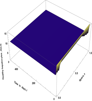
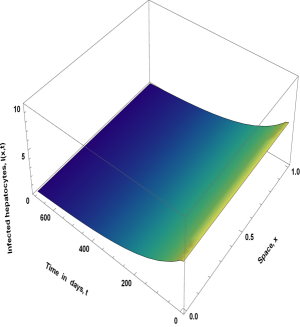
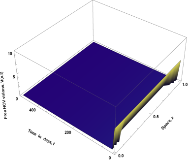
Figure 1: Simulations of IBVP (5) under Neumann boundary conditions (54) and initial condition (55)

Otherwise we choose the numerical values of the parameters for the PDE-cellular model system (5) as follows : $\lambda=50$; $d=5$; $\rho=0,01$; $\alpha=0,05$; $D_{1}=D_{2}=D_{3}=0,1$; $\eta=0,00004$; $\varepsilon=0,5$; $\alpha_{0}=1$; $\alpha_{1}=0,1$; $\alpha_{2}=0,02$; $\alpha_{3}=0,03$; $k=2$; $\mu=2$; $\beta=0,24$ et $u=1$. By calculation we have $\mathcal{R}_{0}=6.25009$. In this case, PDE-cellular model system (5) has a spatially homogeneous equilibrium $E^{*}=(5;500;235)$. Hence by Theorem 4.5 $E^{*}$ is globally asymptotically stable. Numerical simulation illustrates our result (see figure 2).

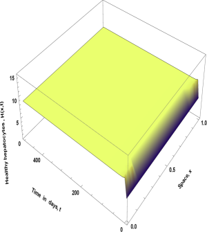
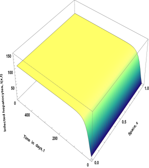
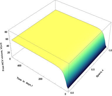
Figure 2: Simulations of IBVP (5) under Neumann boundary conditions (54) and initial condition (56)

Conflict of interest

The authors declare that they have no conflict of interests regarding the publication of this paper.

6 Conclusion

In this work, we addressed the dynamics of a reaction diffusion HCV intra-host infection model with the Hattaf-Yousfi incidence rate, which is a generalized nonlinear incidence rate. The object of this work was to make a mathematical analysis of a cellular model of HCV infection which assumes that virions diffuse into the liver, which uses the Hattaf-Yousfi functional response generalizing most of the functional responses that exist. Our model also takes into account the absorption effect which is much neglected in the literature. We first showed that the initial value and boundary problem (5) admits a unique global solution in time. And secondly, we have shown that this unique solution is positive and uniformly bounded. Then, we gave the expression of basic reproduction number $\mathcal{R}_{0}$ which is the parameter from which we studied the dynamics of our model at equilibria whose existence and uniqueness of these have been previously proven. More precisely, we have shown that, if $\mathcal{R}_{0}<1$, the unique uninfected equilibrium point is locally and globally asymptotically stable. This means that, under this condition,infection disappears. Otherwise, the uninfected equilibrium point is unstable; and in this case the infection persists in the host. It has also been shown under the hypothesis $\mathcal{R}_{0}>1$, that the infected equilibrium point is locally and globally asymptotically stable. This edifying work ended with numerical simulations, carried out on the Mathematica software, which confirmed our theoretical results. In order to get as close as possible to complex reality of biological phenomena, we envisage in the future, the mathematical analysis of models taking into account cell proliferation and the delay.

Appendix A Proof of Proposition 2

The proof is established by using Banach’s Fixed Point Theorem.
Choose $\beta$ such that $\frac{3}{4}<\beta<1$, then the injection $\mathcal{I}:D(\mathcal{H}^{\beta})\rightarrow C_{B}^{0}$ is continuous by Lemma 2. For $r_{0}>0$ and $T>0$, the following closed ball is considered :

$$B_{r_{0}}(H_{0},I_{0},V_{0})=\left\{(H,I,V)\in(C_{B}^{0}(]0,T],D(\mathcal{H}^{\beta})))^{3}:\|H-H_{0}\|_{\beta},\|I-I_{0}\|_{\beta},\|V-V_{0}\|_{\beta}\leq r_{0}\right\}.$$ (57)

By Proposition 1, we have the local Lipschitz properties:

$$\|\mathcal{F}(t,H_{1},I_{1},V_{1})-\mathcal{F}(t,H_{2},I_{2},V_{2})\|_{2} \leq K_{1}^{1}\|H_{1}-H_{2}\|_{D(\mathcal{H}^{\beta})}+K_{2}^{1}\|I_{1}-I_{2}\|_{D(\mathcal{H}^{\beta})}+K_{3}^{1}\|V_{1}-V_{2}\|_{D(\mathcal{H}^{\beta})},$$

$$\|\mathcal{G}(t,H_{1},I_{1},V_{1})-\mathcal{G}(t,H_{2},I_{2},V_{2})\|_{2} \leq K_{1}^{2}\|H_{1}-H_{2}\|_{D(\mathcal{H}^{\beta})}+K_{2}^{2}\|I_{1}-I_{2}\|_{D(\mathcal{H}^{\beta})}+K_{3}^{2}\|V_{1}-V_{2}\|_{D(\mathcal{H}^{\beta})},$$

$$\|\mathcal{Q}(t,H_{1},I_{1},V_{1})-\mathcal{Q}(t,H_{2},I_{2},V_{2})\|_{2} \leq K_{1}^{3}\|H_{1}-H_{2}\|_{D(\mathcal{H}^{\beta})}+K_{2}^{3}\|I_{1}-I_{2}\|_{D(\mathcal{H}^{\beta})}+K_{3}^{3}\|V_{1}-V_{2}\|_{D(\mathcal{H}^{\beta})},$$

for $t\in[0,T]$, $(H_{1},I_{1},V_{1}),(H_{2},I_{2},V_{2})\in B_{r_{0}}(H_{0},I_{0},V_{0})$ and Lipschitz-constants $K_{j}^{i}>0$, $i,j=1,2,3$. In addition $(y_{1},y_{2},y_{3})\in B_{r_{0}}(H_{0},I_{0},V_{0})$, define $P:[0,T]\rightarrow L^{2}(\Omega)$, $Q:[0,T]\rightarrow L^{2}(\Omega)$ and $R:[0,T]\rightarrow L^{2}(\Omega)$ as follows

$$Py_{1}(t) = G_{1}(t)H_{0}+\int_{0}^{t}G_{1}(t-\tau)\mathcal{F}(t,y_{1}(\tau),y_{2}(\tau),y_{3}(\tau))d\tau,$$

$$Qy_{2}(t) = G_{2}(t)I_{0}+\int_{0}^{t}G_{2}(t-\tau)\mathcal{G}(t,y_{1}(\tau),y_{2}(\tau),y_{3}(\tau))d\tau,$$

$$Ry_{3}(t) = G_{3}(t)V_{0}+\int_{0}^{t}G_{3}(t-\tau)\mathcal{Q}(t,y_{1}(\tau),y_{2}(\tau),y_{3}(\tau))d\tau.$$

Finally, set $M_{1}=\sup\limits_{t\in[0,T]}\|\mathcal{F}(t,y_{1}(0),y_{2}(0),y_{3}(0))\|_{2}$, $M_{2}=\sup\limits_{t\in[0,T]}\|\mathcal{G}(t,y_{1}(0),y_{2}(0),y_{3}(0))\|_{2}$, $M_{3}=\sup\limits_{t\in[0,T]}\|\mathcal{Q}(t,y_{1}(0),y_{2}(0),y_{3}(0))\|_{2}$ and choose T so that:

$$\|G_{1}(h)H_{0}-H_{0}\|_{\beta},\|G_{2}(h)I_{0}-I_{0}\|_{\beta},\|G_{3}(h)V_{0}-V_{0}\|_{\beta}\leq\frac{3r_{0}}{4},\;\;0\leq h\leq T,$$ (59)

$$C_{\beta,2}^{i}(M_{i}+r_{0}K_{1}^{i}+r_{0}K_{2}^{i}+r_{0}K_{3}^{i})\int_{0}^{T}s^{-\beta}ds\leq\frac{r_{0}}{4},\;\;i=1,2,3,$$ (60)

where $C_{\beta,2}^{i}$ is the constant in property 2) of Corollary 1 for operator A ($A$ is zero for $i=1$, $2$). Note that such T exists since $G_{1}(h)$, $G_{2}(h)$ and $G_{3}(h)$ converge to $Id$ as $h$ tends to $0^{+}$ by definition of an analytic semigroup and

$$\int_{0}^{T}s^{-\beta}ds=\frac{1}{1-\beta}h^{1-\beta}\rightarrow 0,\;\;h\rightarrow 0^{+}\;\;for\;\;\beta<1.$$

Then the proof will continue according to the following two points :

(a)

it is shown that (P,Q,R) maps $B_{r_{0}}(H_{0},I_{0},V_{0})$ into itself,

(b)

it is shown that (P,Q,R) is a strict contraction on $B_{r_{0}}(H_{0},I_{0},V_{0})$, allowing the use of Banach’s Fixed Point Theorem to get the existence of a unique fixed point in $B_{r_{0}}(H_{0},I_{0},V_{0})$.

Let $(H,I,V)\in B_{r_{0}}(H_{0},I_{0},V_{0})$. Then, using (59) and property 2) of Corollary 1, we have :

$$\|PH(t)-H_{0}\|_{D(\mathcal{H}^{\beta})} = \Big{\|}G_{1}(t)H_{0}-H_{0}+\int_{0}^{t}G_{1}(t-\tau)\mathcal{F}(\tau,H(\tau),I(\tau),V(\tau))d\tau\Big{\|}_{D(\mathcal{H}^{\beta})},$$

$$\leq \|G_{1}(t)H_{0}-H_{0}\|_{D(\mathcal{H}^{\beta})}+\int_{0}^{t}\|G_{1}(t-\tau)\mathcal{F}(\tau,H(\tau),I(\tau),V(\tau))\|_{D(\mathcal{H}^{\beta})}d\tau,$$

$$\leq \frac{3r_{0}}{4}+\int_{0}^{t}C_{\beta,2}^{1}(t-s)^{-\beta}\Big{\|}\mathcal{F}(\tau,H(\tau),I(\tau),V(\tau))\Big{\|}_{2}d\tau,$$

$$\leq \frac{3r_{0}}{4}+\int_{0}^{t}C_{\beta,2}^{1}(t-s)^{-\beta}\Big{\|}\mathcal{F}(\tau,H(\tau),I(\tau),V(\tau))-\mathcal{F}(\tau,H_{0},I_{0},V_{0})+\mathcal{F}(\tau,H_{0},I_{0},V_{0})\Big{\|}_{2}d\tau,$$

$$\leq \frac{3r_{0}}{4}+\int_{0}^{t}C_{\beta,2}^{1}(t-s)^{-\beta}\Big{(}\Big{\|}\mathcal{F}(\tau,H(\tau),I(\tau),V(\tau))-\mathcal{F}(\tau,H_{0},I_{0},V_{0})\Big{\|}_{2}$$

$$+ \Big{\|}\mathcal{F}(\tau,H_{0},I_{0},V_{0})\Big{\|}_{2}\Big{)}d\tau,$$

$$\|PH(t)-H_{0}\|_{D(\mathcal{H}^{\beta})} \leq \frac{3r_{0}}{4}+\int_{0}^{t}C_{\beta,2}^{1}(t-s)^{-\beta}\Big{(}K_{1}^{1}r_{0}+K_{2}^{1}r_{0}+K_{3}^{1}r_{0}+M_{1}\Big{)}d\tau,$$

$$\leq \frac{3r_{0}}{4}+C_{\beta,2}^{1}\left(K_{1}^{1}r_{0}+K_{2}^{1}r_{0}+K_{3}^{1}r_{0}+M_{1}\right)\int_{0}^{t}(t-s)^{-\beta}d\tau,$$

$$\leq \frac{3r_{0}}{4}+0,$$

$$\leq r_{0}\;\;\mbox{for}\;\;0\leq t\leq T,$$

and similarly

$$\|QI(t)-I_{0}\|_{D(\mathcal{H}^{\beta})}\leq r_{0}\;\;\mbox{and}\;\;<\|RV(t)-V_{0}\|_{D(\mathcal{H}^{\beta})}\leq r_{0}.$$

Showing that $(P,Q,R)$ maps $B_{r_{0}}(H_{0},I_{0},V_{0})$ into itself. Furthermore, from property 1) in Corollary 1 and Lemma 3 we compute:

$$\|PH(t+h)-PH(t)\|_{D(\mathcal{H}^{\beta})}$$

$$= \Big{\|}G_{1}(t+h)H_{0}-G_{1}(t)H_{0}+\int_{0}^{t+h}G_{1}(t+h-\tau)\mathcal{F}(\tau,H(\tau),I(\tau),V(\tau))d\tau$$

$$-\int_{0}^{t}G_{1}(t-\tau)\mathcal{F}(\tau,H(\tau),I(\tau),V(\tau))d\tau\Big{\|}_{D(\mathcal{H}^{\beta})},$$

$$= \Big{\|}G_{1}(t)G_{1}(h)H_{0}-G_{1}(t)H_{0}+\int_{0}^{t}G_{1}(h)G_{1}(t-\tau)\mathcal{F}(\tau,H(\tau),I(\tau),V(\tau))d\tau$$

$$+\int_{t}^{t+h}G_{1}(h)G_{1}(t-\tau)\mathcal{F}(\tau,H(\tau),I(\tau),V(\tau))d\tau-\int_{0}^{t}G_{1}(t-\tau)\mathcal{F}(\tau,H(\tau),I(\tau),V(\tau))d\tau\Big{\|}_{D(\mathcal{H}^{\beta})},$$

$$= \Big{\|}G_{1}(t)(G_{1}(h)-Id)H_{0}+\int_{0}^{t}(G_{1}(h)-Id)G_{1}(t-\tau)\mathcal{F}(\tau,H(\tau),I(\tau),V(\tau))d\tau$$

$$+\int_{t}^{t+h}G_{1}(t+h-\tau)\mathcal{F}(\tau,H(\tau),I(\tau),V(\tau))d\tau\Big{\|}_{D(\mathcal{H}^{\beta})}.$$

The strong continuity of the semigroup and Lemma 3 yields

$$\|PH(t+h)-PH(t)\|_{D(\mathcal{H}^{\beta})}\rightarrow 0\;\;\mbox{as}\;\;h\rightarrow 0^{+}.$$

Therefore P is continuous from [0,T] into $D(\mathcal{H}^{\beta})$.
A similar Calculation shows that Q and R have the same properties and item (a) is proved.
Presently let us show that $(P,Q,R)$ is a strict contraction on $B_{r_{0}}(H_{0},I_{0},V_{0})$.
Let $(y_{1},y_{2},y_{3}),\;(z_{1},z_{2},z_{3})\in B_{r_{0}}(H_{0},I_{0},V_{0})$. Then

$$\|Py_{1}(t)-Pz_{1}(t)\|_{D(\mathcal{H}^{\beta})} = \Big{\|}\int_{0}^{t}G_{1}(t-\tau)\Big{(}\mathcal{F}(\tau,y_{1}(\tau),y_{2}(\tau),y_{3}(\tau))-\mathcal{F}(\tau,z_{1}(\tau),z_{2}(\tau),z_{3}(\tau))\Big{)}d\tau\Big{\|}_{D(\mathcal{H}^{\beta})},$$

$$\leq \int_{0}^{t}\Big{\|}G_{1}(t-\tau)\Big{(}\mathcal{F}(\tau,y_{1}(\tau),y_{2}(\tau),y_{3}(\tau))-\mathcal{F}(\tau,z_{1}(\tau),z_{2}(\tau),z_{3}(\tau))\Big{)}\Big{\|}_{D(\mathcal{H}^{\beta})}d\tau,$$

$$\leq \int_{0}^{t}C_{\beta,2}^{1}(t-\tau)^{-\beta}\Big{\|}\mathcal{F}(\tau,y_{1}(\tau),y_{2}(\tau),y_{3}(\tau))-\mathcal{F}(\tau,z_{1}(\tau),z_{2}(\tau),z_{3}(\tau))\Big{\|}_{2}d\tau,$$

$$\leq \int_{0}^{t}C_{\beta,2}^{1}(t-\tau)^{-\beta}\Big{(}K_{1}^{1}\|y_{1}-z_{1}\|_{D(\mathcal{H}^{\beta})}+K_{2}^{1}\|y_{2}-z_{2}\|_{D(\mathcal{H}^{\beta})}+K_{3}^{1}\|y_{3}-z_{3}\|_{D(\mathcal{H}^{\beta})}\Big{)}d\tau,$$

$$\leq C_{\beta,2}^{1}\Big{(}K_{1}^{1}\sup_{\tau\in[0,t]}\|y_{1}-z_{1}\|_{D(\mathcal{H}^{\beta})}+K_{2}^{1}\sup_{\tau\in[0,t]}\|y_{2}-z_{2}\|_{D(\mathcal{H}^{\beta})}$$

$$+ K_{3}^{1}\sup_{\tau\in[0,t]}\|y_{3}-z_{3}\|_{D(\mathcal{H}^{\beta})}\Big{)}\int_{0}^{t}(t-\tau)^{-\beta}d\tau.$$

That is :

$$\|Py_{1}(t)-Pz_{1}(t)\|_{D(\mathcal{H}^{\beta})}$$

$$\leq C_{\beta,2}^{1}\Big{(}K_{1}^{1}+K_{2}^{1}+K_{3}^{1}+\frac{M_{1}}{r_{0}}\Big{)}\Big{(}\sup_{\tau\in[0,t]}\|y_{1}-z_{1}\|_{D(\mathcal{H}^{\beta})}+\sup_{\tau\in[0,t]}\|y_{2}-z_{2}\|_{D(\mathcal{H}^{\beta})}$$

$$+\sup_{\tau\in[0,t]}\|y_{3}-z_{3}\|_{D(\mathcal{H}^{\beta})}\Big{)}\int_{0}^{t}(t-\tau)^{-\beta}d\tau,$$

$$\leq \Big{(}\sup_{\tau\in[0,t]}\|y_{1}-z_{1}\|_{D(\mathcal{H}^{\beta})}+\sup_{\tau\in[0,t]}\|y_{2}-z_{2}\|_{D(\mathcal{H}^{\beta})}+\sup_{\tau\in[0,t]}\|y_{3}-z_{3}\|_{D(\mathcal{H}^{\beta})}\Big{)}$$

$$\times C_{\beta,2}^{1}\Big{(}K_{1}^{1}+K_{2}^{1}+K_{3}^{1}+\frac{M_{1}}{r_{0}}\Big{)}\int_{0}^{t}s^{-\beta}ds,$$

$$\leq \Big{(}\sup_{\tau\in[0,t]}\|y_{1}-z_{1}\|_{D(\mathcal{H}^{\beta})}+\sup_{\tau\in[0,t]}\|y_{2}-z_{2}\|_{D(\mathcal{H}^{\beta})}+\sup_{\tau\in[0,t]}\|y_{3}-z_{3}\|_{D(\mathcal{H}^{\beta})}\Big{)}$$

$$\times\frac{1}{r_{0}}C_{\beta,2}^{1}\left(r_{0}K_{1}^{1}+r_{0}K_{2}^{1}+r_{0}K_{3}^{1}+M_{1}\right)\int_{0}^{T}s^{-\beta}ds,$$

$$\leq \Big{(}\sup_{\tau\in[0,t]}\|y_{1}-z_{1}\|_{D(\mathcal{H}^{\beta})}+\sup_{\tau\in[0,t]}\|y_{2}-z_{2}\|_{D(\mathcal{H}^{\beta})}+\sup_{\tau\in[0,t]}\|y_{3}-z_{3}\|_{D(\mathcal{H}^{\beta})}\Big{)}\frac{1}{r_{0}}\times\frac{r_{0}}{4},$$

$$\leq \frac{1}{4}\Big{(}\sup_{\tau\in[0,t]}\|y_{1}-z_{1}\|_{D(\mathcal{H}^{\beta})}+\sup_{\tau\in[0,t]}\|y_{2}-z_{2}\|_{D(\mathcal{H}^{\beta})}+\sup_{\tau\in[0,t]}\|y_{3}-z_{3}\|_{D(\mathcal{H}^{\beta})}\Big{)},$$

for every $t\in[0,T]$. Hence

$$\sup_{t\in[0,T]}\|Py_{1}(t)-Pz_{1}(t)\|_{D(\mathcal{H}^{\beta})} \leq \frac{1}{4}\Big{(}\sup_{\tau\in[0,t]}\|y_{1}-z_{1}\|_{D(\mathcal{H}^{\beta})}+\sup_{\tau\in[0,t]}\|y_{2}-z_{2}\|_{D(\mathcal{H}^{\beta})}+\sup_{\tau\in[0,t]}\|y_{3}-z_{3}\|_{D(\mathcal{H}^{\beta})}\Big{)}.$$

Similarly

$$\sup_{t\in[0,T]}\|Qy_{1}(t)-Qz_{1}(t)\|_{D(\mathcal{H}^{\beta})} \leq \frac{1}{4}\Big{(}\sup_{\tau\in[0,t]}\|y_{1}-z_{1}\|_{D(\mathcal{H}^{\beta})}+\sup_{\tau\in[0,t]}\|y_{2}-z_{2}\|_{D(\mathcal{H}^{\beta})}+\sup_{\tau\in[0,t]}\|y_{3}-z_{3}\|_{D(\mathcal{H}^{\beta})}\Big{)}$$

and

$$\sup_{t\in[0,T]}\|Ry_{1}(t)-Rz_{1}(t)\|_{D(\mathcal{H}^{\beta})} \leq \frac{1}{4}\Big{(}\sup_{\tau\in[0,t]}\|y_{1}-z_{1}\|_{D(\mathcal{H}^{\beta})}+\sup_{\tau\in[0,t]}\|y_{2}-z_{2}\|_{D(\mathcal{H}^{\beta})}+\sup_{\tau\in[0,t]}\|y_{3}-z_{3}\|_{D(\mathcal{H}^{\beta})}\Big{)}.$$

Thus

$$\sup\limits_{t\in[0,T]}\|(P,Q,R)(y_{1}(t),y_{2}(t),y_{3}(t))-(P,Q,R)(z_{1}(t),z_{2}(t),z_{3}(t))\|_{D(\mathcal{H}^{\beta})^{3}}$$

$$\leq \sup_{\tau\in[0,t]}\Big{(}\|Py_{1}-Pz_{1}\|_{D(\mathcal{H}^{\beta})}+\|Qy_{2}-Qz_{2}\|_{D(\mathcal{H}^{\beta})}+\|Ry_{3}-Rz_{3}\|_{D(\mathcal{H}^{\beta})}\Big{)},$$

$$\leq \sup_{\tau\in[0,t]}\|Py_{1}-Pz_{1}\|_{D(\mathcal{H}^{\beta})}+\sup_{\tau\in[0,t]}\|Qy_{2}-Qz_{2}\|_{D(\mathcal{H}^{\beta})}+\sup_{\tau\in[0,t]}\|Ry_{3}-Rz_{3}\|_{D(\mathcal{H}^{\beta})},$$

$$\leq \frac{3}{4}\Big{(}\sup_{\tau\in[0,t]}\|y_{1}-z_{1}\|_{D(\mathcal{H}^{\beta})}+\sup_{\tau\in[0,t]}\|y_{2}-z_{2}\|_{D(\mathcal{H}^{\beta})}+\sup_{\tau\in[0,t]}\|y_{3}-z_{3}\|_{D(\mathcal{H}^{\beta})}\Big{)},$$

$$\leq \frac{3}{4}\sup_{t\in[0,T]}\|(y_{1}(t),y_{2}(t),y_{3}(t))-(z_{1}(t),z_{2}(t),z_{3}(t))\|_{D(\mathcal{H}^{\beta})^{3}}.$$

Hence $(P,Q,R)$ is a strict contraction on $B_{r_{0}}(H_{0},I_{0},V_{0})$ and this proves Part b). According to Banach’s Fixed Point Theorem, (P,Q,R) has a unique fixed point in $B_{r_{0}}(H_{0},I_{0},V_{0})$. This is the solution of (5) on [0,T] with initial value $(H(0),I(0),V(0))=(H_{0},I_{0},V_{0})$ in $(D(\mathcal{H}^{\beta}))^{3}$. This completes the proof of Proposition 2.

Appendix B Proof of Theorem 3.3

We first prove the existence and positivity of the solution. From Theorem 3.2, there exist a sequence $(w^{m})$ and a function $w$ such that

$$w^{m}\rightarrow w\;\;\mbox{in}\;\;C([0,T],\mathcal{H}),$$

with $w\geq 0$ and $w(0)=w_{0}$.
We check that

$$q(w^{m-1})\rightarrow q(w)\;\;\mbox{and}\;\;q(w^{m-1})w^{m}\rightarrow q(w)w\;\;\mbox{in}\;\;C([0,T],\mathcal{H}).$$

We also have

$$f(w^{m-1})\rightarrow f(w)\;\;\mbox{in}\;\;C([0,T],\mathcal{H})\bigcap L^{2}((0,T),E^{\prime}).$$

But, $w^{m}$ is solution of

$$\Big{<}\frac{\partial w^{m}}{\partial t},v\Big{>}+\Big{<}Aw^{m},v\Big{>}+\left(q(w^{m-1})w^{m},v\right)=\Big{<}f(w^{m-1}),v\Big{>},\;\;\forall v\in E.$$ (61)

We take $\phi\in\mathcal{D}((0,T))$, so that $\phi v\in L^{2}((0,T),E)$,

$$\int_{0}^{T}\Big{<}\frac{\partial w^{m}}{\partial t},\phi v\Big{>}dt+\int_{0}^{T}\Big{<}Aw^{m},\phi v\Big{>}dt+\int_{0}^{T}\left(q(w^{m-1})w^{m},\phi v\right)dt=\int_{0}^{T}\Big{<}f(w^{m-1}),\phi v\Big{>}dt.$$ (62)

The second term in the left side and the right side of the equality (62) converges due to the weak convergence in $L^{2}((0,T),E^{\prime})$. The third term in the left-hand side of (62) also converges, due to the convergence in $C([0,T],\mathcal{H})$. We deduce that $\frac{\partial w^{m}}{\partial t}$ converges weakly in $L^{2}((0,T),E^{\prime})$.
But we have

$$w^{m}\rightarrow w\;\;\mbox{in}\;\;C([0,T],\mathcal{H}).$$

Then

$$\frac{\partial w^{m}}{\partial t}\rightarrow\frac{\partial w}{\partial t}\;\;\mbox{in}\;\;\mathcal{D^{\prime}}((0,T),\mathcal{H})$$

Therefore, we obtain

$$\frac{\partial w^{m}}{\partial t}\rightarrow\frac{\partial w}{\partial t}\;\;\mbox{weakly in}\;\;L^{2}((0,T),E^{\prime}),$$

and

$$\int_{0}^{T}\Big{<}\frac{\partial w}{\partial t},\phi v\Big{>}dt+\int_{0}^{T}\Big{<}Aw,\phi v\Big{>}dt+\int_{0}^{T}\Big{(}q(w)w,\phi v\Big{)}_{\mathcal{H}}dt=\int_{0}^{T}\Big{<}f(w),\phi v\Big{>}dt.$$ (63)

This being true for all $\phi$, one has

$$\Big{<}\frac{\partial w}{\partial t},v\Big{>}+\Big{<}Aw,v\Big{>}+\Big{(}q(w)w,v\Big{)}_{\mathcal{H}}=\Big{<}f(w),v\Big{>},\;\;\forall v\in E.$$

That is to say,

$$\frac{d}{dt}(w,v)_{\mathcal{H}}+a(w,v)+\Big{(}q(w)w,v\Big{)}_{\mathcal{H}}=\Big{<}f(w),v\Big{>},\;\forall v\in E,$$ (64)

$$\frac{\partial w}{\partial t}=f(w)-Aw-q(w)w\;\;\mbox{in}\;\;L^{2}((0,T),E^{\prime}).$$ (65)

According to (34) and (35) we have

$$w^{m}(t) = G(t)w_{0}+\int_{0}^{t}G(t-s)(-q(w^{m-1})w^{m}+f(w^{m-1}))(s)ds,$$ (66)

and in addition, as $q(w^{m-1})w^{m}$ and $f(w^{m-1})$ converge in $C^{0}([0,T],\mathcal{H})$ and the operator $\mathcal{G}$, defined by the relation (36), is compact, using the limit in (66) one has,

$$w(t) = G(t)w_{0}+\int_{0}^{t}G(t-s)(-q(w)w+f(w))(s)ds.$$ (67)

It remains to prove uniqueness.
Let $v$ be another solution of IBVP (3.3). Then

$$v\in W(0,T,E,E^{\prime})\Rightarrow v\in C([0,T],\mathcal{H})\;\;\mbox{and}\;\;v\geq 0.$$

Consequently we obtain

$$q(v)v+f(v)\in L^{2}((0,T),E^{\prime}).$$

Thus, by Proposition 2.11 of WS , one has

$$v(t) = G(t)w_{0}+\int_{0}^{t}G(t-s)(-q(v)v+f(v))(s)ds.$$

Subtracting, we have

$$w(t)-v(t)=\int_{0}^{t}G(t-s)\Big{(}-(q(w)w-q(v)v)+(f(w)-f(v))\Big{)}(s)ds,$$ (68)

with

$$q(w)w-q(v)v = q(w)w-q(w)v+q(w)v-q(v)v,$$

$$= q(w)(w-v)+(q(w)-q(v))v.$$

Since $w$ is positive, one has

$$\Bigg{\|}\frac{w_{j}}{\alpha_{0}+\alpha_{1}w_{k}+\alpha_{2}w_{j}+\alpha_{3}w_{k}w_{j}}\Bigg{\|}\leq\frac{1}{K}\|w_{j}\|_{\infty}$$

where

$$\|w_{j}\|_{\infty}=\|w_{j}\|_{L^{\infty}((0,T),\mathcal{H})}.$$

If we define

$$\|w\|_{\infty}=\sum_{j=1}^{3}\|w_{j}\|_{\infty},$$

there is $M_{1}>0$ such that

$$\|q(w)\|_{\infty}\leq M_{1}\|w_{j}\|_{\infty}.$$

So, for $r=1,2,3$, the numerator of $q_{r}(w)-q_{r}(v)$ is the sum of terms of the form $(w_{k}-v_{k})v_{j}$ or $(w_{j}-v_{j})w_{k}$, and we can find $M_{2}>0$ such that

$$\big{|}q_{r}(w)-q_{r}(v)\big{|}_{\mathcal{H}}(s)\leq M_{2}\Big{(}\sum_{j=1}^{3}|w_{j}(s)-v_{j}(s)|_{\mathcal{H}}\Big{)}.$$

Also we can find $M_{3}>0$ such that

$$\big{|}f_{r}(w)-f_{r}(v)\big{|}_{\mathcal{H}}(s)\leq M_{3}\Big{(}\sum_{j=1}^{3}|w_{j}(s)-v_{j}(s)|_{\mathcal{H}}\Big{)}.$$

Summing up $|w_{j}(s)-v_{j}(s)|_{\mathcal{H}}$ and noting that $\|G_{j}(t-s)\|\leq N_{j}e^{\theta_{j}T}$ with $N_{j},\;\theta_{j}>0$, we can find $M>0$ such that

$$\sum_{j=1}^{3}|w_{j}(s)-v_{j}(s)|_{\mathcal{H}}\leq M\|w-v\|_{\infty}.$$

Replacing in (68), we obtain

$$\sum_{j=1}^{3}|w_{j}(s)-v_{j}(s)|_{\mathcal{H}}\leq M^{2}\|w-v\|_{\infty}\int_{0}^{t}sds=M^{2}\frac{t^{2}}{2}\|w-v\|_{\infty}.$$

By induction, we have

$$\sum_{j=1}^{3}|w_{j}(s)-v_{j}(s)|_{\mathcal{H}}\leq\frac{M^{n}}{n!}T^{n}\|w-v\|_{\infty},$$

with

$$\lim_{n\rightarrow+\infty}\frac{M^{n}}{n!}T^{n}\|w-v\|_{\infty}=0.$$

Therefore $w=v$. This ends the proof of Theorem 3.3.

References

• (1) Adams R. A.: Sobolev spaces, Academic Press, New York, (1975)
• (2) Amann H.: Dynamic theory of quasilinear parabolic equations-I. Abstract evolution equations, Nonlinear Analysis-Theory, Methods and Applications, 12, 895-919 (1988)
• (3) Amann H.: Dynamic theory of quasilinear parabolic systems-III. Global existence, Math. Z., 202, 219-250 (1989)
• (4) Amann H.: Dynamic theory of quasilinear parabolic equations-II. Reaction-diffusion systems, Differential Integral Equations, 3, 13-75 (1990)
• (5) Beddington J. R.: Mutual interference between parasites or predators and its effect on searching efficiency. J Anim Ecol, 44, 331–340 (1975)
• (6) Chatterjee, A., Guedj, J., Perelson, A. S.: Mathematical modelling of HCV infection: what can it teach us in the era of direct-acting antiviral agents? Antiviral Therapy, 17(6PtB), 1171-1182 (2012). http://dx.doi.org/10.3851/IMP2428
• (7) Chong M. S. F., Crossley L. S. M., Madzvamuse: The stability analyses of the mathematical models of hepatitis C virus infection. Modern Applied Science, 9 (3) 250-271. ISSN 1913-1844, Article (Published Version) Anotida (2015), 23 pages. http://sro.sussex.ac.uk/52312/
• (8) Ciupe S. M., Ribeiro R. M., Nelson P. W., Perelson A. S.: Modeling the mechanisms of acute hepatitis B virus infection. J Theor Biol 247:23–35 (2007)
• (9) Crowley P. H., Martin E. K.: Functional responses and interference within and between year classes of a dragon y population. J N Am Benth Soc, 8, 211–221 (1989)
• (10) Dahari H., Ribeiro R. M., and Perelson A. S.: Triphasic decline of HCV RNA during antiviral therapy, Hepatology, 46, 16–21(2007)
• (11) DeAngelis D.L. , Goldstein R. A. , O’Neill R. V.: A model for trophic interaction. Ecology, 56, 881–892 (1975)
• (12) Goudjo C., Leye B., Sy M.: Weak Solution to a Parabolic Nonlinear System Arising in Biological Dynamic in the Soil, 24 pages (2011), Article ID 831436
• (13) Gourley S. A., So J. W. H.: Dynamics of a food-limited population model with incorporating nonlocal delays on a finite domain, Journal of Mathematical Biology, 44, 49-78 (2002)
• (14) Guedj, J., Neumann, A. U.: Understanding hepatitis C viral dynamics with direct-acting antiviral agents due to the interplay between intracellular replication and cellular infection dynamics. Journal of Theoretical Biology, 267(3), 330-340 (2010). http://dx.doi.org/10.1016/j.jtbi.2010.08.036
• (15) Hattaf K., Yousfi N.: Global stability for reaction-diffusion equations in biology, Computers and Mathematics with Applications, 66, 1488-1497 (2013)
• (16) Hattaf K., Yousfi N.: Global stability of a virus dynamics model with cure rate and absorption, Journal of the Egyptian Mathematical Society, 22, 386-389 (2014)
• (17) Hattaf K., Yousfi N.: Global dynamics of a delay reaction–diffusion model for viral infection with specific functional response. Comp. Appl. Math., 34, 807–818 (2015). DOI 10.1007/s40314-014-0143-x
• (18) Hattaf K., Yousfi N.: A class of delayed viral infection models with general incidence rate and adaptative immune response. Int. J. Dyn, 4(3), 254–265 (2016)
• (19) Hattaf K., Yousfi N., Tridane A.: Mathematical analysis of a virus dynamics model with general incidence rate and cure rate. Nonlinear Anal RWA 13, 1866–1872 (2012)
• (20) Hattaf K., Yousfi N., Tridane A.: A Delay virus dynamics model with general incidence rate. Differ Equ Dyn Syst, (2013). doi:10.1007/s12591-013-0167-5
• (21) Hattaf K., Yousfi N., Tridane A.: Stability analysis of a virus dynamics model with general incidence rate and two delays. Appl Math Comput, 221, 514–521 (2013)
• (22) Henry D.: Geometric Theory of Semilinear Parabolic Equations, 1st edition, Springer-Verlag, (1981)
• (23) Henry D.: Geometric theory of semilinear parabolic equations 840 of Lecture Notes in Mathematic, New york, USA (1993)
• (24) Hollis S. L., Martin R. H., Pierre M.: Global existence and boundedness in reaction-diffusion systems, Siam J. Math. Anal. 18 , 744-761 (1987)
• (25) Huang G., Ma W., Takeuchi Y.: Global properties for virus dynamics model with Beddington–DeAngelis functional response. Appl Math Lett, 22, 1690–1693 (2009)
• (26) Huang G, Ma W., Takeuchi Y.: Global analysis for delay virus dynamics model with Beddington– DeAngelis functional response. Appl Math Lett 24(7), 1199–1203 (2011)
• (27) Khalil, H.: Nonlinear Systems, 3rd edn. Prentice Hall, New York, (2002)
• (28) Li D., Ma W.: Asymptotic properties of an HIV-1 infection model with time delay. J Math Anal Appl, 335, 683–691 (2007)
• (29) Min L., Su y., Kuang Y.: Mathematical analysis of a basic model of virus infection with application to HBV infection, Rocky Mountain J. Math. 38(5), 1573–1585 (2008)
• (30) Neumann A. U., Lam H., Dahari D. R., Gretch T. E., Wiley T. J., Layden A. S.: Hepatitis C viral dynamics in vivo and the antiviral efficacy of interferon-$\alpha$ therapy. Science, 282:103–107 (1998)
• (31) Nowak M. A., Bangham C. R. M.: Population dynamics of immune responses to persistent viruses, Science, 272 , 74-79 (1996)
• (32) Nowak M. A., Bonhoeffer S., Hill A. M., Boehme R., Thomas H. C., McDade H.: Viral dynamics in hepatitis B virus infection, Proceedings of the National Academy of Sciences, 93, 4398-4402 (1996)
• (33) Protter M. H., Weinberger H. P.: Maximum principle in differential equations. Prentice-Hall, Englewood Cliffs, New Jersey, USA(1967)
• (34) Riad D., Hattaf K., Yousfi N.: Dynamics of capital-labour model with Hattaf-Yousfi functional response. J. Adv. Math. Comput. Sci 18(5) 329, 1–7 (2016)
• (35) Rong, L., Perelson, A. S. :Mathematical analysis of multiscale models for hepatitis C virus dynamics under therapy with direct-acting antiviral agents. Mathematical Biosciences, 245(1), 22-30 (2013). http://dx.doi.org/10.1016/j.mbs.2013.04.012
• (36) Song X., Neumann A.: Global stability and periodic solution of the viral dynamics. J Math Anal Appl, 329, 281–297 (2007)
• (37) Thieme HR.: Spectral bound and reproduction number for infinite-dimensional population structure and time heterogeneity, SIAM J. Appl. Math. 70, 188-211 (2009)
• (38) Wang X., Tao Y., Song X.: Global stability of a virus dynamics model with Beddington–DeAngelis incidence rate and CTL immune response. Nonlinear Dyn, 66, 825–830 (2011)
• (39) Wang K., Wang W.: Propagation of HBV with spatial dependence, Mathematical Biosciences, 210, 78-95 (2007)
• (40) Wang W., Zhao X.-Q.: Basic reproduction numbers for reactiondiffusion epidemic models, SIAM J. APPL. Dyn. Syst. 11, 1652-1673 (2012)
• (41) WHO: Global hepatitis report. Geneva: World Health Organization; 2017 (http://apps.who.int/iris/bitstream/10665/255016/1/9789241565455- eng.pdf?ua=1, accessed 29 January 2018) (2017)
• (42) Zhang Y., Xu Z.: Dynamics of a diffusive HBV model with delayed Beddington–DeAngelis response. Real world applications: nonlinear analysis, (2013)
• (43) Zhou X., Cui J.: Global stability of the viral dynamics with crowley–martin functional response. Bull Korean Math Soc, 48(3), 555–574 (2011)