New Hard-thresholding Rules based on Data Splitting in High-dimensional Imbalanced Classification

Abstract

In binary classification, imbalance refers to situations in which one class is heavily under-represented. This issue is due to either a data collection process or because one class is indeed rare in a population. Imbalanced classification frequently arises in applications such as biology, medicine, engineering, and social sciences. In this paper, for the first time, we theoretically study the impact of imbalance class sizes on the linear discriminant analysis (LDA) in high dimensions. We show that due to data scarcity in one class, referred to as the minority class, and high-dimensionality of the feature space, the LDA ignores the minority class yielding a maximum misclassification rate. We then propose a new construction of hard-thresholding rules based on a data splitting technique that reduces the large difference between the misclassification rates. We show that the proposed method is asymptotically optimal. We further study two well-known sparse versions of the LDA in imbalanced cases. We evaluate the finite-sample performance of different methods using simulations and by analyzing two real data sets. The results show that our method either outperforms its competitors or has comparable performance based on a much smaller subset of selected features, while being computationally more efficient.

KEY WORDS: Classification, High-dimensionality, Imbalanced, Linear Discriminant Analysis, Thresholding.

1 Introduction

The rise of high-dimensional data has affected many areas of research in statistics and machine learning, including classification. Linear Discriminant Analysis (LDA) has been extensively studied in high-dimensional classification. Bickel and Levina (2004), Fan and Fan (2008), and Shao et al. (2011) showed that when the number of features is larger than the sample size, the LDA can perform as badly as a random guess. To deal with the curse of dimensionality, several developments have been made over the last decade or so. For example, among others, new developments include the nearest shrunken centroids Tibshirani et al. (2002), shrunken centroids regularized discriminant analysis Guo et al. (2006), features annealed independence rule (fair) Fan and Fan (2008), sparse and penalized LDA Shao et al. (2011); Witten and Tibshirani (2011), regularized optimal affine discriminant (road) Fan et al. (2012), multi-group sparse discriminant analysis Gaynanova et al. (2015), pairwise sure independent screening Pan et al. (2016), and the ultra high-dimensional multiclass LDA Li et al. (2019). The general idea of these methods is to incorporate a feature selection strategy in a classifier in order to obtain certain optimality properties in the sense of misclassification rates.

To the best of our knowledge, most of the existing developments in high dimensions focus on problems with comparable class sizes in the training data. However, in applications such as clinical diagnosis (Bach et al., 2017), fraud detection (Bolton and Hand, 2002), drug discovery (Zhu et al., 2006), or equipment malfunction detection (Park et al., 2013), classification often suffers from imbalanced class sizes where, for example, in a binary problem one class (referred to as the minority class) is heavily under-represented. This is due to either a data collection process or because one class is indeed rare in a population. In such situations, the minority class is of primary interest as it carries substantial information, and often has higher misclassification costs compared to the larger class, referred to as the majority class. For example, in a study of a certain rare disease, the cost of misclassifying a positive case is often higher than the cost of misclassifying a negative one (Ramaswamy et al., 2002). In banking or telecommunication studies, few customers are voluntarily willing to terminate their contracts and leave their provider. In these applications, misclassification of a potential churner is more expensive than that of a non-churner for a provider (Verbeke et al., 2012). Due to data scarcity in the minority class, conventional discriminant methods are often biased toward the majority class resulting in much higher misclassification rate for the minority class. This error dramatically increases in high-dimensional cases, as empirically shown by Blagus and Lusa (2010). In this paper, we study imbalanced binary classification with the class sizes $n_{2}<<n_{1}$, when the number of features, $p_{n}$, grows to infinity as the total sample size $n=(n_{1}+n_{2})$ grows to infinity. We refer to Class 1 with size $n_{1}$ as the majority class, and Class 2 with size $n_{2}$ as the minority class. A specific limiting relationship between $n_{1}$ and $n_{2}$ is given in Section 2.2.

Imbalanced classification under various settings have attracted attention in recent years. A common approach to deal with the imbalanced issue is to make virtual class sizes comparable by using resampling methods, for example, the synthetic minority over-sampling technique (smote) of (Chawla et al., 2002). The recent work of Feng et al. (2020) provides a review of the common re-sampling techniques for fixed dimensional imbalanced problems. In other methods, such as the weighted extreme learning machine Zong et al. (2013) and the cost-sensitive support vector machine (svm) Iranmehr et al. (2019), the idea is to strengthen the relative impact of the minority class by either assigning different weights to sample units or different costs to misclassification instances in each class. Bak and Jensen (2016) studied distributional properties of the correct classification probabilities of the minority and majority classes of a hard-thresholding independence rule. Using a non-asymptotic approach, they adjusted the bias of correct classification probabilities which is rooted on the imbalanced class sizes. Huang et al. (2010) and Pang et al. (2013) proposed bias-corrected discriminant functions. Owen (2007) studied limiting form of the logistic regression under a so-called infinitely imbalanced case in which the size of one class is fixed and the other grows to infinity. Qiao and Liu (2009) proposed new evaluation criteria and weighted learning procedures that increase the impact of a minority class. Qiao et al. (2010) developed a distance weighted discrimination method (dwd), originally proposed to overcome the well-known data-piling issue Ahn and Marron (2010) in high-dimensions, by an adaptive weighting scheme to reduce sensitivity to unequal class sizes. Qiao and Zhang (2013) proposed a linear classifier that is a hybrid of dwd and svm, thus haivng advantages of both techniques. Qiao and Zhang (2015) introduced a new family of classifiers including svm and dwd that provides a trade-off between imbalanced and high-dimensionality. Hall et al. (2005); Nakayama et al. (2017) theoretically showed that under certain conditions, svm suffers from data-piling in high-dimensions, meaning that all data points become the support vectors which may result in ignorance of one of the classes. Nakayama et al. (2017) proposed a biased-corrected svm that improves its performance even when the class sizes are imbalanced. Nakayama (2020) proposed a robust svm which is less sensitive to class sizes and choice of a regularization parameter. Xie et al. (2020) used a repeated case-control sampling technique coupled with a fused feature screening procedure to deal with imbalanced and high-dimensionality.

The behaviour of LDA in high-dimensional imbalanced classification has often been studied empirically. In this paper, we first theoretically show that in such cases this classifier ignores the minority class, yielding a maximum misclassification rate for this class. On the other hand, a common approach to deal with high-dimensionality is to use a hard-thresholding operator for feature selection. However, our simulations show large differences between the misclassification rates of the hard-thresholding rule (hr) in imbalanced settings. Thus, we face both high-dimensionality and an inflated bias in the difference between the two misclassification rates. To address the issues, we propose a new construction of the hr based a multiple data splitting (Msplit) technique as described below, and thus called Msplit-hr. We randomly split the training data in each class into two parts of sizes $\lfloor n_{k}/2\rfloor,k=1,2$, and use one part only for feature selection and the other part is then used to construct a bias-corrected classifier based on the selected features. As shown in Section 3, the splitting facilitates the correction of the inflated bias in the difference between the two misclassification rates. To reduce the effect of randomness in single-split, we repeat the process several ($\mathcal{L}$) times which maximizes the usage of training data in finite-sample situations. In general, as pointed out by Meinshausen et al. (2009), multiple splitting also helps reproducibility of finite sample results. As shown numerically in Figures 1 and 2, respectively discussed in Sections 3.1 and 3.2, the classification results of Msplit-hr corresponding to $\mathcal{L}\approx 30$ are unsurprisingly more powerful than a single-split ($\mathcal{L}=1$). We show that our method is asymptotically optimal. We also study asymptotic properties of two well-known linear classifiers, namely the sparse LDA Shao et al. (2011), and the regularized optimal affine discriminant analysis Fan et al. (2012), under the imbalanced setting. Our simulations show that Msplit-hr either outperforms its competitors or has comparable performance based on a much smaller subset of selected features, while being computationally more efficient as discussed in Section 5.

The rest of the paper is organized as follows. Section 2 gives the problem setup and investigates the behaviour of the LDA in high-dimensional imbalanced binary classification. Section 3 introduces our proposed method, Msplit-hr. Large-sample properties of the method are also discussed in this section. Two well-known high-dimensional variants of the LDA, under the imbalanced setting, are studied in Section 4. The finite-sample performance of several binary classifiers is examined using simulations in Section 5. Analysis of two real data sets are given in Section 6. A summary and discussion are given in Section 7. Technical Lemmas and proofs of our main results are given in Appendices A-C.

Notation: All vectors and matrices are shown in bold letters. For any vector $\textbf{a}\in\mathbb{R}^{p}$, $\|\textbf{a}\|_{0}=\#\{j:\ a_{j}\neq 0\}$, $\|\textbf{a}\|_{1}=\sum_{j=1}^{p}|a_{j}|$, $\|\textbf{a}\|_{2}=(\sum_{j=1}^{p}a_{j}^{2})^{1/2}$, $\|\textbf{a}\|_{\infty}=\max_{j=1,...,p}|a_{j}|$. For any symmetric matrix $\textbf{A}\in\mathbb{R}^{p\times p}~{}$, $\|\textbf{A}\|_{1}=\max_{i=1,...,p}\sum_{j=1}^{p}|a_{ij}|$, $\|\textbf{A}\|=\max_{j=1,...,p}|\lambda_{j}(\textbf{A})|$, where $\lambda_{j}(\textbf{A})$ are the eigenvalues of the matrix A, and $\|\textbf{A}\|_{\infty}=\max_{i,j=1,...,p}|a_{ij}|$. A diagonal matrix is denoted by D. For any two sequences $a_{n}$ and $b_{n}$, we write $a_{n}\lesssim b_{n}$ or $a_{n}=O(b_{n})$, if for sufficiently large $n$ there exists a constant $C$ such that $a_{n}\leq C~{}b_{n}$. We write $a_{n}\sim b_{n}$, if $a_{n}/b_{n}\to 1$, as $n\to\infty$. And $a_{n}\asymp b_{n}$, if $a_{n}=O(b_{n})$ and $b_{n}=O(a_{n})$. Also, $a_{n}=o(b_{n})$, when $a_{n}/b_{n}\rightarrow 0$ as $n\rightarrow\infty$. The notations $o_{p}$ and $O_{p}$ are respectively used to indicate convergence and boundedness in probability. An indicator function is denoted by $\textbf{1}\{\cdot\}$.

2 The LDA

In this section, we first describe the setting of the binary classification problem under our consideration. We then study the effect of dimension and imbalanced class sizes on the LDA, which motives the topics of the remaining sections.

2.1 Overview

We consider the class labels $Y\in\{1,2\}$, class prior probabilities $\pi_{k}=\Pr(Y=k)$, and a $p$-dimensional feature vector $\textbf{X}=(X_{1},X_{2},\ldots,X_{p})^{\top}$ such that $\textbf{X}|Y=k\sim N_{p}(\mbox{\boldmath$\mu$}_{k},\mbox{\boldmath$\Sigma$}),k=1,2.$ The LDA is a well-known classification technique for this setting. More specifically, given the parameter vector $\boldsymbol{\theta}=(\mbox{\boldmath$\mu$}_{1},\mbox{\boldmath$\mu$}_{2},\mbox{\boldmath$\Sigma$})$ and assuming $\pi_{1}=\pi_{2}$, the optimal rule classifies a subject with an observed feature vector $\textbf{x}^{*}=(x^{*}_{1},\ldots,x^{*}_{p})^{\top}$ to Class 1 if and only if

$$\delta^{\text{opt}}(\textbf{x}^{*};\boldsymbol{\theta})=\mbox{\boldmath$\mu$}_{d}^{\top}\mbox{\boldmath$\Sigma$}^{-1}(\textbf{x}^{*}-\mbox{\boldmath$\mu$}_{a})<0,$$ (2.1)

where $\mbox{\boldmath$\mu$}_{d}=\mbox{\boldmath$\mu$}_{2}-\mbox{\boldmath$\mu$}_{1}\neq\mbox{\boldmath$0$}$, $\mbox{\boldmath$\mu$}_{a}=(\mbox{\boldmath$\mu$}_{2}+\mbox{\boldmath$\mu$}_{1})/2$.

The misclassification rate (MCR) of a classifier is typically used to quantity its performance. The classifier in (2.1) which is the Bayes’ rule, is referred to as the optimal rule since it has the smallest average MCR, $\Pi^{\text{opt}}$ in (2.2) below, among all classifiers. For $\delta^{\text{opt}}$, the class-specific MCRs are equal and given by

$$\Pi_{k}=\Pr\bigg{(}(-1)^{k}\delta^{\text{opt}}(\textbf{X}^{*};\boldsymbol{\theta})<0\bigg{|}Y=k\bigg{)}=\Phi\left(-\Delta_{p}/2\right)\equiv\Pi^{\text{opt}},\ \ k=1,2,$$ (2.2)

where $\Phi$ is the cumulative distribution function of the standard normal, and $\Delta_{p}^{2}=\mbox{\boldmath$\mu$}_{d}^{\top}\mbox{\boldmath$\Sigma$}^{-1}\mbox{\boldmath$\mu$}_{d}$ is referred to as the discriminative power or signal value. It is seen that as $\Delta_{p}\to\infty$, high discriminative power, then $\Pi^{\text{opt}}\to 0$; and as $\Delta_{p}\to 0$, low discriminative power, then $\Pi^{\text{opt}}\to\frac{1}{2}$ implying that the classifier performs as a random guess. From now on, we assess the performance of other classifiers under consideration by comparing them with the optimal rule.

In practice, the parameter vector $\boldsymbol{\theta}$ is unknown and needs to be estimated using a training data $\mathcal{D}_{n}=\{\textbf{x}_{ik},\ i=1,...,n_{k},\ k=1,2\}$, where $\textbf{x}_{ik}$ is the $i$-th observed value of X in Class $k$, and the $n_{k}$ are the class sample sizes with the total sample size $n=n_{1}+n_{2}$. For a new feature vector $\textbf{x}^{*}$, a so-called plug-in discriminant function based on the parameter estimates is given by

$$\delta^{\text{\sc lda}}(\textbf{x}^{*};\widehat{\boldsymbol{\theta}}_{n})=\widehat{\mbox{\boldmath$\mu$}}_{d}^{\top}~{}\widehat{\mbox{\boldmath$\Sigma$}}_{n}^{-1}(\textbf{x}^{*}-\widehat{\mbox{\boldmath$\mu$}}_{a}),$$ (2.3)

where $\widehat{\boldsymbol{\theta}}_{n}=(\widehat{\mbox{\boldmath$\mu$}}_{n,1},\widehat{\mbox{\boldmath$\mu$}}_{n,2},\widehat{\mbox{\boldmath$\Sigma$}}_{n})$ and

$$\widehat{\mbox{\boldmath$\mu$}}_{n,k}\equiv\widehat{\mbox{\boldmath$\mu$}}_{k} = \frac{1}{n_{k}}\sum_{i=1}^{n_{k}}\textbf{x}_{ik},\ \ k=1,2,$$ (2.4)

$$\widehat{\mbox{\boldmath$\Sigma$}}_{n} = \frac{1}{n-2}\sum_{k=1}^{2}\sum_{i=1}^{n_{k}}(\textbf{x}_{ik}-\widehat{\mbox{\boldmath$\mu$}}_{k})(\textbf{x}_{ik}-\widehat{\mbox{\boldmath$\mu$}}_{k})^{\top}.$$ (2.5)

The matrix $\widehat{\mbox{\boldmath$\Sigma$}}^{-1}_{n}$ in (2.3) is a generalized inverse when $\widehat{\mbox{\boldmath$\Sigma$}}_{n}$ is not invertible. Given $\mathcal{D}_{n}$, the conditional MCR of the plug-in linear discriminant rule based on (2.3) corresponding to Class $k\in\{1,2\}$, is given by

$$\Pi_{k}^{\text{\sc lda}}(\mathcal{D}_{n})=\Pr\left((-1)^{k}\delta^{\text{\sc lda}}(\textbf{X}^{*};\widehat{\boldsymbol{\theta}}_{n})<0\bigg{|}\ Y=k,\ \mathcal{D}_{n}\right)=\Phi\bigg{(}\frac{\Psi_{k}^{\text{\sc lda}}(\widehat{\boldsymbol{\theta}}_{n})}{\sqrt{\Upsilon^{\text{\sc lda}}(\widehat{\boldsymbol{\theta}}_{n})}}\bigg{)},$$ (2.6)

where $\Psi_{k}^{\text{\sc lda}}(\widehat{\boldsymbol{\theta}}_{n})=(-1)^{k}\widehat{\mbox{\boldmath$\mu$}}_{d}^{\top}\widehat{\mbox{\boldmath$\Sigma$}}_{n}^{-1}(\widehat{\mbox{\boldmath$\mu$}}_{a}-\mbox{\boldmath$\mu$}_{k})$, and $\Upsilon^{\text{\sc lda}}(\widehat{\boldsymbol{\theta}}_{n})=\widehat{\mbox{\boldmath$\mu$}}_{d}^{\top}\widehat{\mbox{\boldmath$\Sigma$}}_{n}^{-1}\mbox{\boldmath$\Sigma$}\widehat{\mbox{\boldmath$\Sigma$}}_{n}^{-1}\widehat{\mbox{\boldmath$\mu$}}_{d}$. As is common in the literature, we study large-sample properties of a classifier through its conditional MCR.

2.2 Impact of the dimension and imbalanced class sizes

The effect of the dimension $p$ on the LDA’s performance is well studied in the literature. Shao et al. (2011) showed that when $p$ is fixed or diverges to infinity at a slower rate than $\sqrt{n}$, the classifier is asymptotically optimal (Shao et al., 2011, Definition 1). When $p\rightarrow\infty$ such that $p/n\rightarrow\infty$, Bickel and Levina (2004), Fan and Fan (2008), and Shao et al. (2011) showed that this classifier performs no better than a random guess. Hence, feature selection is essential when $p$ is large compared to the sample size $n$.

In the aforementioned works, the impact of dimensionality is studied under particular limiting settings on the class sizes $n_{1}$ and $n_{2}$. Bickel and Levina (2004) and Shao et al. (2011) respectively considered equal class sizes ($n_{1}=n_{2}$) and unequal sizes where $n_{1},\ n_{2}\rightarrow\infty$ such that $\frac{n_{2}}{n}\rightarrow\pi$, $0<\pi<1$. Fan and Fan (2008) developed their results by considering compatible class sizes, such that $c_{1}\leq\frac{n_{1}}{n_{2}}\leq c_{2}$, with $0<c_{1}\leq c_{2}<\infty$. Bak and Jensen (2016) investigated the case where $n_{1},\ n_{2}\rightarrow\infty$, such that $\frac{n_{1}-n_{2}}{n_{1}+n_{2}}=\rho>0$ is fixed. All in all, it is seen that the sizes of the two classes grow similarly and proportional to the total sample size $n$, that is $n_{k}=O(n),k=1,2$. We refer to these settings as a balanced classification problem. Owen (2007) analyzed the binary logistic regression models with fixed dimension $p$ in a so-called infinitely imbalanced case in which $n_{1}\rightarrow\infty$ but the class size $n_{2}$ is fixed. In this paper, we study imbalanced classification in which $n_{1}$ and $n_{2}$ grow to infinity such that $n_{2}=o(n_{1})$, implying a different growth rate of the class sizes.

In the balanced classification, typically average (over the two classes) MCR (Shao et al., 2011; Fan et al., 2012) or the MCR of one arbitrary class (Bickel and Levina, 2004; Fan and Fan, 2008) is used as a performance measure of a classifier. However, in imbalanced situations due to data scarcity in the minority class, classification results have a tendency to favour the majority class. Thus, the average MCR is not an appropriate performance measure for a classifier ${\cal T}$. This motivated us to adapt the optimality definition of a classifier from Shao et al. (2011) to our setting as follows.

Definition 1

Suppose ${\cal T}$ is a classifier in a binary classification problem. The misclassification rates of ${\cal T}$, given the training data ${\cal D}_{n}$, are denoted by $\Pi_{k}^{{\cal T}}({\cal D}_{n}),k=1,2$. Then,

1. $\cal T$ is asymptotically-strong optimal if $\Pi_{k}^{\cal T}({\cal D}_{n})/\Pi^{\text{opt}}\overset{p}{\longrightarrow}1$, $k=1,2$,

2. $\cal T$ is asymptotically-strong sub-optimal if $\Pi_{k}^{\cal T}({\cal D}_{n})-\Pi^{\text{opt}}\overset{p}{\longrightarrow}0$, $k=1,2$,

3. $\cal T$ is asymptotically-strong worst if $\Pi_{k}^{\cal T}({\cal D}_{n})\overset{p}{\longrightarrow}\frac{1}{2}$, $k=1,2$,

4. $\cal T$ is asymptotically ignorant if $\min_{k=1,2}\Pi_{k}^{\cal T}({\cal D}_{n})\overset{p}{\longrightarrow}0$ and
   $\max_{k=1,2}\Pi_{k}^{\cal T}({\cal D}_{n})\overset{p}{\longrightarrow}1$.

Note that any classifier ${\cal T}$ satisfying either of the properties in parts (i)-(iii) of the above definition also satisfies the properties discussed in the corresponding parts of Definition 1 of Shao et al. (2011) for a balanced case, but not vice versa. Part (iv) of the above definition occurs when a classifier completely ignores one of the classes, and more specifically the minority class. We now state our first result.

Theorem 2.1

Suppose that the estimator $\widehat{\mbox{\boldmath$\Sigma$}}_{n}^{-1}$ in $\delta^{\text{\sc lda}}$ in (2.3) is replaced by $\mbox{\boldmath$\Sigma$}^{-1}$, and $\Sigma$ is known. When $n_{2}=o(n_{1})$, such that $p/n_{2}\to\infty$ and $\sqrt{\frac{n_{2}}{p}}\Delta_{p}^{2}=o(1)$, as $n_{1},n_{2}\to\infty$, then the LDA is asymptotically ignorant, that is,

$$\Pi_{1}^{\text{\sc lda}}(\mathcal{D}_{n})\overset{p}{\longrightarrow}\ 0~{}~{},~{}~{}\Pi_{2}^{\text{\sc lda}}(\mathcal{D}_{n})\overset{p}{\longrightarrow}\ 1.$$

This result implies that in the high-dimensional imbalanced cases, the MCR of the majority class tends to 0 which will be even better than the optimal value $\Pi^{\text{opt}}$, but the MCR of the minority class approaches 1 which is worse than a random guess. Note that the above result also holds in the case of $p/n_{1}\to c$, for some finite constant $c\geq 0$. (Hall et al., 2005; Nakayama et al., 2017) showed that, under certain conditions, the svm ignores the minority class in high-dimensional imbalanced problems.

Remark 2.1

When $p$ is fixed and $n_{2}=o(n_{1})$, then the LDA is asymptotically-strong optimal.

Remark 2.1 illustrates that in the fixed-dimensional case, the impact of imbalanced class sizes asymptotically vanishes and $\Pi_{k}^{\text{\sc lda}}(\mathcal{D}_{n}),~{}k=1,2$, converge to the optimal value $\Pi^{\text{opt}}$. Hence, by Theorem 2.1, Shao’s results, and Remark 2.1, the effects of both dimension and imbalanced class sizes are responsible for ignorance of the minority class.

3 Proposed Method: Msplit hard-thresholding rule (Msplit-hr)

A common approach to deal with high-dimensionality in the LDA is to incorporate feature selection using a hard-thresholding rule (hr) based on a two-sample t-statistic as in Fan and Fan (2008). More specifically, by ignoring the correlation among features, $\Sigma$ is estimated by the diagonal matrix $\widehat{\textbf{D}}_{n}=diag\{\widehat{\sigma}_{1}^{2},...,\widehat{\sigma}_{p}^{2}\}$, and the discriminant function is given by

$$\delta^{\text{\sc hr}}(\textbf{x}^{*};\widehat{\boldsymbol{\theta}}_{n})=\sum_{j=1}^{p}r_{j}(\textbf{x}^{*};\widehat{\boldsymbol{\theta}}_{n})~{}h_{j}(\widehat{\boldsymbol{\theta}}_{n}),$$ (3.1)

where $\widehat{\boldsymbol{\theta}}_{n}=(\widehat{\boldsymbol{\mu}}_{1},\widehat{\boldsymbol{\mu}}_{2},\widehat{\textbf{D}}_{n})$, $r_{j}(\textbf{x}^{*};\widehat{\boldsymbol{\theta}}_{n})=(\widehat{\mu}_{dj}/\widehat{\sigma}_{j}^{2})(x_{j}^{*}-\widehat{\mu}_{aj})$, and $h_{j}(\widehat{\boldsymbol{\theta}}_{n})=\textbf{1}\{|t_{j}|>\tau_{n}\}$ is the thresholding operator based on the t-statistic

$$t_{j}=\frac{\widehat{\mu}_{j2}-\widehat{\mu}_{j1}}{\widehat{\sigma}_{j}\sqrt{n/n_{1}n_{2}}}.$$ (3.2)

Here $\widehat{\mu}_{jk}$’s and $\widehat{\sigma}_{j}^{2}$’s are the entries of $\widehat{\boldsymbol{\mu}}_{k}$ and $\widehat{\mbox{\boldmath$\Sigma$}}_{n}$ in (2.4) and (2.5), respectively. The discriminant function of FAIR proposed by Fan and Fan (2008) for balanced problems belongs to the class of functions in (3.1). The authors select an optimal number of statistically most significant features, or equivalently the threshold value $\tau_{n}$ of t-statistic, by minimizing a common upper bound on its corresponding MCRs. However, for the case of general $\Sigma$, such choice of $\tau_{n}$ does not necessarily result in an asymptotically optimal classifier Shao et al. (2011). Thus, for generality, in the rest of the paper, for any given sequence of $\tau_{n}$, we refer to a classifier based on (3.1) as an HR unless otherwise is specified.

If indeed $\mbox{\boldmath$\Sigma$}=\textbf{D}$, Bak and Jensen (2016) showed that the hr in (3.1) based on a fixed threshold $\tau_{n}=\tau$, is asymptotically ignorant when $\rho=(n_{1}-n_{2})/(n_{1}+n_{2})>0$ is fixed, as $n_{1},n_{2}\to\infty$. As stated after Theorem 3.1 below, it is interesting to note that under the imbalanced setting $n_{2}=o(n_{1})$ and by an appropriate choice of $\tau_{n}$, the hr is indeed asymptotically-strong optimal. However, our simulations in Section 5 show an unsatisfactory finite-sample performance of the hr in the sense of both the MCR in the minority class and large difference between the two MCRs. We propose a new construction of the hr which outperforms (3.1) in finite-samples, while maintaining the same desirable large-sample properties, to be discussed below. To fix ideas, we first consider the imbalanced problem with a diagonal $\mbox{\boldmath$\Sigma$}=\textbf{D}$. The general case of a non-diagonal $\Sigma$ is discussed in Subsection 3.2, which is based on a feature screening technique. Note that under this case, the hr based on (3.1) is not optimal, as it ignores the correlation among the features.

3.1 Msplit-HR under a diagonal $\Sigma$

As discussed in Section 2, the class specific MCRs of the optimal rule are equal, and are given in (2.2). Our numerical experiments show that, due to the imbalanced class sizes, hr performs well in majority class but underperforms in minority class, though it has large-sample optimal property as discussed after Theorem 3.1 below. Thus, the idea in our work is to reduce the difference between two conditional MCRs of hr toward that of the optimal rule which is zero. More specifically, our main goal is to propose a new discriminant function aiming to reduce the difference between the MCRs of the hr,

$$|\Pi_{1}^{\text{\sc hr}}(\mathcal{D}_{n})-\Pi_{2}^{\text{\sc hr}}(\mathcal{D}_{n})|=|\Phi({\psi}_{1,n})-\Phi({\psi}_{2,n})|,$$

where $\psi_{k,n}=\Psi_{k}^{\text{\sc hr}}(\widehat{\boldsymbol{\theta}}_{n})/\surd\Upsilon^{\text{\sc hr}}(\widehat{\boldsymbol{\theta}}_{n})$ and

$$\begin{matrix}\Psi_{k}^{\text{\sc hr}}(\widehat{\boldsymbol{\theta}}_{n})=(-1)^{k+1}\sum_{j=1}^{p}r_{j}(\mbox{\boldmath$\mu$}_{k};\widehat{\boldsymbol{\theta}}_{n})h_{j}(\widehat{\boldsymbol{\theta}}_{n})~{},~{}\Upsilon^{\text{\sc hr}}(\widehat{\boldsymbol{\theta}}_{n})=\sum_{j=1}^{p}(\widehat{\mu}_{dj}/\widehat{\sigma}_{j}^{2})^{2}\sigma_{j}^{2}h_{j}(\widehat{\boldsymbol{\theta}}_{n})\end{matrix}$$

for $k=1,2$. To understand the above difference, Bak and Jensen (2016) studied distributional properties of the quantities $\psi_{k,n},k=1,2$. They focused on reducing the so-called bias

$$B_{n}^{\text{\sc hr}}=\mathbb{E}\big{\{}\Psi_{1}^{\text{\sc hr}}(\widehat{\boldsymbol{\theta}}_{n})-\Psi_{2}^{\text{\sc hr}}(\widehat{\boldsymbol{\theta}}_{n})\big{\}}$$ (3.3)

to zero, which results in decreasing the bias between $\psi_{1,n}$ and $\psi_{2,n}$ and consequently of that between MCRs. However, it turns out that due to the dependency between the random variables $r_{j}$ and $h_{j}$, computing $B_{n}^{\text{\sc hr}}$ is not an easy task. Bak and Jensen (2016) studied the origin of the bias and proposed methods for its correction. We instead propose a new construction of the hr that facilities the computation of such bias by adapting a sample-splitting strategy as follows.

The training sample of each class is randomly partitioned into two sub-samples of sizes $n^{\prime}_{k}=\lfloor n_{k}/2\rfloor$. The two sub-samples are used for computing two quantities similar to the $r_{j}$ and $h_{j}$ in (3.1), for each $j=1,\ldots,p$, and then the results are merged. To reduce the effect of randomness due to the data splitting, this process is repeated, say, $\mathcal{L}$ times. Our new discrimination function is then constructed by averaging over the hr-type discriminant functions based on each splitting. Thus, we chose the name Msplit-hr for our method. More specifically, at the $\ell$-th data splitting, for each $\ell=1,...,\mathcal{L}$, the entire training data $\mathcal{D}_{n}$ is partitioned into two parts $\mathcal{D}_{n,\ell}^{(1)}$ and $\mathcal{D}_{n,\ell}^{(2)}$. The parameter estimates based on each sub-sample are distinguished by the superscripts ⁽¹⁾ and ⁽²⁾, that is, $\widehat{\boldsymbol{\theta}}_{n,\ell}^{(1)}$ and $\widehat{\boldsymbol{\theta}}_{n,\ell}^{(2)}$. A new observation with a feature vector $\textbf{x}^{*}$ is then classified using the discriminant function

$$\delta_{0}^{\text{Msplit-{\sc hr}}}(\textbf{x}^{*};\widehat{\boldsymbol{\theta}}_{n})=\frac{1}{\mathcal{L}}\sum_{\ell=1}^{\mathcal{L}}\sum_{j=1}^{p}r_{j}(\textbf{x}^{*};\widehat{\boldsymbol{\theta}}_{n,\ell}^{(2)})~{}h_{j}(\widehat{\boldsymbol{\theta}}_{n,\ell}^{(1)}),$$ (3.4)

where $\widehat{\boldsymbol{\theta}}_{n}=\{(\widehat{\boldsymbol{\theta}}_{n,\ell}^{(1)},\widehat{\boldsymbol{\theta}}_{n,\ell}^{(2)}):~{}\text{for }\ell=1,\dots,\mathcal{L}\}$. Due to the statistical independence of the two random functions $h_{j}$ and $r_{j}$ in (3.4), for all $j=1,\ldots,p$, calculation of the bias $B_{n}$ for $\delta_{0}^{\text{Msplit-{\sc hr}}}$ is straight forward, which is shown below. Recall $n^{\prime}_{k}=\lfloor n_{k}/2\rfloor$, and let $n^{\prime}=n^{\prime}_{1}+n^{\prime}_{2}$ and $f_{n^{\prime}}=n^{\prime}/2-1$.

Proposition 3.1

The bias $B_{n}$ in (3.3) corresponding to $\delta_{0}^{\text{Msplit-{\sc hr}}}$ is given by

$$B_{0,n}^{\text{Msplit-{\sc hr}}}=\mathbb{E}\big{\{}\Psi_{0,1}^{\text{Msplit-{\sc hr}}}(\widehat{\boldsymbol{\theta}}_{n})-\Psi_{0,2}^{\text{Msplit-{\sc hr}}}(\widehat{\boldsymbol{\theta}}_{n})\big{\}}=\frac{\bar{r}_{n}}{\mathcal{L}}\sum_{\ell=1}^{\mathcal{L}}\sum_{j=1}^{p}\mathbb{E}\{h_{j}(\widehat{\boldsymbol{\theta}}_{n,\ell}^{(1)})\},$$

where $\bar{r}_{n}=f_{n^{\prime}}(\frac{1}{n^{\prime}_{1}}-\frac{1}{n^{\prime}_{2}})\frac{\Gamma(f_{n^{\prime}}-1)}{\Gamma(f_{n^{\prime}})}$, and $\Gamma(\cdot)$ is the gamma function.

Finally, using the above result, we propose the bias-corrected discriminant function

$$\delta^{\text{Msplit-{\sc hr}}}(\textbf{x}^{*};\widehat{\boldsymbol{\theta}}_{n})=\frac{1}{\mathcal{L}}\sum_{\ell=1}^{\mathcal{L}}\sum_{j=1}^{p}\bigg{\{}r_{j}(\textbf{x}^{*};\widehat{\boldsymbol{\theta}}_{n,\ell}^{(2)})-\frac{\bar{r}_{n}}{2}\bigg{\}}h_{j}(\widehat{\boldsymbol{\theta}}_{n,\ell}^{(1)})$$ (3.5)

which has its bias $B_{n}^{\text{Msplit-{\sc hr}}}=0$. The term $\bar{r}_{n}$ is a function of $(n^{\prime}_{2}-n^{\prime}_{1})$ which is negative since $n_{2}<n_{1}$. Hence, for any new feature vector $\textbf{x}^{*}$, the resulting discriminant function (3.5) tends to be more positive compared to the rule in (3.4). This increases the chance (or probability) of classifying a new observation to the minority class, and hence improving the classification results for this class. In our simulations and the real-data analysis, we evaluate the performance of Msplit-hr based on the bias corrected function $\delta^{\text{Msplit-{\sc hr}}}$. We now describe Algorithm 1 that summarizes the steps for computing (3.5).

Algorithm 1 : Computing the discriminant function $\delta^{\text{Msplit-{\sc hr}}}$.

0:  Input $n^{\prime}_{1}=\lfloor n_{1}/2\rfloor,n^{\prime}_{2}=\lfloor n_{2}/2\rfloor,\textbf{x}^{*},\mathcal{L},\bar{r}_{n}$ and $\tau_{n}$.

1:  for $\ell=1,\dots,\mathcal{L}$ do

2:     Split $\mathcal{D}_{n}$ into $\mathcal{D}_{n,\ell}^{(1)}$ and $\mathcal{D}_{n,\ell}^{(2)}$

3:     for $j=1,\dots,p$ do

4:        Step1: Using $\mathcal{D}_{n,\ell}^{(1)}$ compute $h_{j}(\widehat{\boldsymbol{\theta}}_{n,\ell}^{(1)})$

5:        Step2: Using $\mathcal{D}_{n,\ell}^{(2)}$ compute $r_{j}(\textbf{x}^{*};\widehat{\boldsymbol{\theta}}_{n,\ell}^{(2)})-\frac{\bar{r}_{n}}{2}$

6:     end for

7:  end for

8:  return  $\delta^{\text{Msplit-HR}}(\textbf{x}^{*};\widehat{\boldsymbol{\theta}}_{n})=\frac{1}{\mathcal{L}}\sum_{\ell=1}^{\mathcal{L}}\sum_{j=1}^{p}\bigg{\{}r_{j}(\textbf{x}^{*};\widehat{\boldsymbol{\theta}}_{n,\ell}^{(2)})-\frac{\bar{r}_{n}}{2}\bigg{\}}h_{j}(\widehat{\boldsymbol{\theta}}_{n,\ell}^{(1)})$.

In practice, a value of $\mathcal{L}$ is required to compute (3.5). Figure 1 shows the class-specific MCRs of (3.5) as a function of $\mathcal{L}$, corresponding to scenario (i) in our simulations in Section 5.1. It can be seen that a value of $\mathcal{L}$ between 20 to 30 provides a satisfactory performance of Msplit-hr. We used $\mathcal{L}=30$ in our numerical experiments.

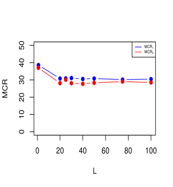
(a) $n_{1}=50$, $n_{2}=10$

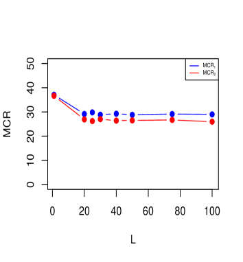
(b) $n_{1}=100$, $n_{2}=10$

Figure 1: Effect of the number of sample-splits $\mathcal{L}$ on Msplit-hr performance for the Simulation setting (i) and $p=1000$.

The following results show the asymptotic behaviour of $\delta^{\text{Msplit-{\sc hr}}}$. First, we state Lemma 3.1 that provides conditions under which the t-statistic (3.2) used in the thresholding operator $h_{j}$ in $\delta^{\text{Msplit-{\sc hr}}}$ selects all the important features. Since $\mathcal{L}$ is fixed, the result of the lemma holds for all $\ell=1,\dots,\mathcal{L}$.

Lemma 3.1

Assume that the mean difference vector $\mbox{\boldmath$\mu$}_{d}=\mbox{\boldmath$\mu$}_{2}-\mbox{\boldmath$\mu$}_{1}$ is sparse. Let $\mathcal{S}=\{j:\mu_{dj}\neq 0\}$ be the the corresponding active set with the cardinality $s=|\mathcal{S}|$, and define $d_{0,n}=\min_{j\in\mathcal{S}}|\mu_{dj}|$. Under Conditions (C1) and (C2) in Appendix A, if $\tau_{n}=O(\sqrt{n_{2}}d_{0,n})$, $\log s=o(n_{2}d_{0,n}^{2})$, $\log(p-s)=o(\tau_{n}^{2})$, $n_{2}=o(n_{1})$, and $\sqrt{n_{2}}d_{0,n}\to\infty$, as $n_{1},n_{2}\to\infty$, then

$$(a) \Pr\bigg{(}\bigcap_{j\not\in\mathcal{S}}\{|t_{j}|\leq\tau_{n}\}\bigg{)}\to 1;~{}~{}(b)~{}~{}\Pr\bigg{(}\bigcap_{j\in\mathcal{S}}\{|t_{j}|>\tau_{n}\}\bigg{)}\to 1.$$

In the above Lemma, if $d_{0,n}=d_{0}$, for some constant $d_{0}>0$, then $\tau_{n}=O(\sqrt{n_{2}})$ and $\log p=o(n_{2})$. On the other hand, if $d_{0,n}\sim n_{2}^{-\gamma}\alpha_{n_{2}}$, for $0<\gamma<1$ and some $\alpha_{n_{2}}\to\infty$, such that $d_{0,n}$ declines to zero and $\sqrt{n_{2}}d_{0,n}\to\infty$, then we have $\tau_{n}=O(n_{2}^{1/2-\gamma}\alpha_{n_{2}})$ and $\log p=o(n_{2}^{1-2\gamma}\alpha_{n_{2}}^{2})$. Therefore, in both cases the divergence rate of the dimension $p$ is smaller than that of the minority class size $n_{2}$, as opposed to the balanced case where $\log p=o(n)$, that is, a larger dimension $p$ allowance.

Theorem 3.1

Suppose that the conditions of Lemma 3.1 are satisfied.
Let $\kappa_{n}=\max\{\Delta_{p}^{-1}\sqrt{s/n_{2}}~{},~{}\sqrt{\log p/n_{1}}\}$. For any fixed $\mathcal{L}$,

• the MCRs of Msplit-hr are given by

  $$\Pi_{k}^{\text{Msplit-{\sc hr}}}(\mathcal{D}_{n})=\Phi\bigg{(}-\frac{1}{2}\Delta_{p}(1+O_{p}(\kappa_{n}))\bigg{)},~{}~{}k=1,2$$

• if $s\Delta_{p}^{2}=o(n_{2})$ and $\Delta_{p}^{2}\sqrt{\log p/n_{1}}=o(1)$, the Msplit-hr is asymptotically-strong optimal.

Note that the result of Theorem 3.1 also holds for the hr. Part (b) of the theorem implies that the growth rates of both the sparsity size $s$ and the discriminative power $\Delta_{p}$ are controlled by the minority class size $n_{2}$.

3.2 Msplit-HR under a general $\Sigma$

When the dimension $p$ is large compared to the sample size $n$, the sample covariance matrix in (2.5) is ill-conditioned. To deal with the singularity issue, many existing methods in the literature involve a feature selection strategy. In what follows, we use a variable screening method (Fan and Lv, 2008; Pan et al., 2016) to select a subset of features $x_{j}$’s that have the highest discriminative power.

At the $\ell$-th data splitting stage of Msplit-hr, we consider the mean difference estimators $\widehat{\boldsymbol{\mu}}_{d,\ell}^{(1)}=\widehat{\mbox{\boldmath$\mu$}}_{2,\ell}^{(1)}-\widehat{\mbox{\boldmath$\mu$}}_{1,\ell}^{(1)}$, which are computed based on the training sub-samples $\mathcal{D}_{n,\ell}^{(1)}$, for $\ell=1,...,\mathcal{L}$. For a given threshold parameter $\tau_{n}$, we select those features $x_{j}$ whose indices belong to the set $\mathcal{S}^{(1)}_{n,\ell}=\{1\leq j\leq p:|\widehat{\mu}_{dj,\ell}^{(1)}|>\tau_{n}\}$, where $\widehat{\mu}_{dj,\ell}^{(1)}$ is the $j$-th entry of $\widehat{\boldsymbol{\mu}}_{d,\ell}^{(1)}$.

For any $p$-dimensional feature vector $\textbf{x}^{*}$, we define the discriminant function

$$\delta_{0}^{\text{Msplit-{\sc hr}}}(\textbf{x}^{*};\widehat{\boldsymbol{\theta}}_{n})=\frac{1}{\mathcal{L}}\sum_{\ell=1}^{\mathcal{L}}\tilde{\boldsymbol{\mu}}_{d,\ell}^{\top}\widetilde{\mbox{\boldmath$\Sigma$}}^{-1}_{n,\ell}~{}(\textbf{x}_{\ell}^{*}-\tilde{\boldsymbol{\mu}}_{a,\ell}),$$ (3.6)

where $\widehat{\boldsymbol{\theta}}_{n}$ is the vector of corresponding parameter estimates, and $\textbf{x}_{\ell}^{*}=(x_{j}^{*}:j\in\mathcal{S}^{(1)}_{n,\ell})^{\top}$ are sub-vectors of the full feature vector $\textbf{x}^{*}$. Furthermore, for all $\ell=1,\ldots,\mathcal{L}$, we have $\tilde{\mbox{\boldmath$\mu$}}_{d,\ell}=\tilde{\mbox{\boldmath$\mu$}}_{2,\ell}-\tilde{\mbox{\boldmath$\mu$}}_{1,\ell}$, $\tilde{\mbox{\boldmath$\mu$}}_{a,\ell}=(\tilde{\mbox{\boldmath$\mu$}}_{1,\ell}+\tilde{\mbox{\boldmath$\mu$}}_{2,\ell})/2$, such that $\tilde{\mbox{\boldmath$\mu$}}_{k,\ell}=(\widehat{\mu}_{jk,\ell}^{(2)}:j\in\mathcal{S}^{(1)}_{n,\ell})^{\top}$ for $k=1,2$, and $\widetilde{\mbox{\boldmath$\Sigma$}}_{n,\ell}=[{\widehat{\sigma}_{jj^{\prime},\ell}^{(2)}}:j,j^{\prime}\in\mathcal{S}^{(1)}_{n,\ell}]$ are respectively the sub-vectors and sub-matrices of the sample means and covariance matrix given in (2.4) and (2.5). Note that for the existence of $\widetilde{\mbox{\boldmath$\Sigma$}}^{-1}_{n,\ell}$, for all $\ell=1,2,\ldots,\mathcal{L}$, we include at most $(n^{\prime}-2)$ features in each $\mathcal{S}_{n,\ell}^{(1)}$.

As discussed in Subsection 3.1, the data splitting technique facilitates computation of the bias $B_{n}$ (3.3) corresponding to (3.6).

Proposition 3.2

If $|\mathcal{S}_{n,\ell}^{(1)}|<n^{\prime}-3$, for all $\ell=1,..,\mathcal{L}$, then

$$B_{0,n}^{\text{Msplit-{\sc hr}}}=\mathbb{E}\{\Psi_{0,1}^{\text{Msplit-{\sc hr}}}(\widehat{\boldsymbol{\theta}}_{n})-\Psi_{0,2}^{\text{Msplit-{\sc hr}}}(\widehat{\boldsymbol{\theta}}_{n})\}=\frac{1}{\mathcal{L}}\sum_{\ell=1}^{\mathcal{L}}\mathbb{E}\{\bar{r}_{n,\ell}\},$$

where

$$\bar{r}_{n,\ell}=\bigg{(}\frac{1}{n^{\prime}_{1}}-\frac{1}{n^{\prime}_{2}}\bigg{)}\frac{n^{\prime}-2}{n^{\prime}-3-|\mathcal{S}_{n,\ell}^{(1)}|}\times|\mathcal{S}_{n,\ell}^{(1)}|.$$ (3.7)

Finally, our bias-corrected discriminant function is

$$\delta^{\text{Msplit-{\sc hr}}}(\textbf{x}^{*};\widehat{\boldsymbol{\theta}}_{n})=\frac{1}{\mathcal{L}}\sum_{\ell=1}^{\mathcal{L}}\{\tilde{\boldsymbol{\mu}}_{d,\ell}^{\top}\tilde{\boldsymbol{\Sigma}}_{n,\ell}^{-1}(\textbf{x}_{\ell}^{*}-\tilde{\boldsymbol{\mu}}_{a,\ell})-\frac{\bar{r}_{n,\ell}}{2}\}$$ (3.8)

which has its bias $B_{n}^{\text{Msplit-{\sc hr}}}=0$. The term $\bar{r}_{n,\ell}$ as a function of $(n^{\prime}_{2}-n^{\prime}_{1})$ makes the corrected discriminant function (3.8) more positive compared to the rule in (3.6). This increases the probability of classifying a new observation to the minority class, and hence improving the results for this class. Algorithm 2 below summarize the steps for computing in (3.8).

Figure 2 shows the class-specific MCRs of (3.8) as a function of $\mathcal{L}$, corresponding to scenario (iv) in our simulations in Section 5.2. Based on these results, we used $\mathcal{L}=30$ in our numerical experiments.

Algorithm 2 Computing the discriminant function in (3.8)

0:  Input $n^{\prime}_{1}=\lfloor n_{1}/2\rfloor,n^{\prime}_{2}=\lfloor n_{2}/2\rfloor,\textbf{x}^{*},\mathcal{L}$, and $\tau_{n}$.

1:  for $\ell=1,\dots,\mathcal{L}$ do

2:     Split $\mathcal{D}_{n}$ into $\mathcal{D}_{n,\ell}^{(1)}$ and $\mathcal{D}_{n,\ell}^{(2)}$

3:     Using $\mathcal{D}_{n,\ell}^{(1)}$, obtain $\mathcal{S}^{(1)}_{n,\ell}=\{1\leq j\leq p:|\widehat{\mu}_{dj,\ell}^{(1)}|>\tau_{n}\}$ and compute $\bar{r}_{n,\ell}$ in (3.7)

4:     if $|\mathcal{S}_{n,\ell}^{(1)}|<n^{\prime}_{1}+n^{\prime}_{2}-3$ then

5:        Using $\mathcal{S}^{(1)}_{n,\ell}$ and $\mathcal{D}_{n,\ell}^{(2)}$, compute $\tilde{\boldsymbol{\mu}}_{d,\ell}^{\top}\tilde{\boldsymbol{\Sigma}}_{n,\ell}^{-1}(\textbf{x}_{\ell}^{*}-\tilde{\boldsymbol{\mu}}_{a,\ell})$

6:     else

7:        Step 1: Select the first $(n^{\prime}_{1}+n^{\prime}_{2}-4)$ features in $\mathcal{S}_{n,\ell}^{(1)}$ with highest value of $|\widehat{\mu}_{dj,\ell}^{(1)}|$

8:        Step 2: Using $\mathcal{D}_{n,\ell}^{(2)}$ and the selected features in Step 1, compute $\tilde{\boldsymbol{\mu}}_{d,\ell}^{\top}\tilde{\boldsymbol{\Sigma}}_{n,\ell}^{-1}(\textbf{x}_{\ell}^{*}-\tilde{\boldsymbol{\mu}}_{a,\ell})$

9:     end if

10:  end for

11:  return  $\delta^{\text{Msplit-HR}}(\textbf{x}^{*};\widehat{\boldsymbol{\theta}}_{n})=\frac{1}{\mathcal{L}}\sum_{\ell=1}^{\mathcal{L}}\{\tilde{\boldsymbol{\mu}}_{d,\ell}^{\top}\tilde{\boldsymbol{\Sigma}}_{n,\ell}^{-1}(\textbf{x}_{\ell}^{*}-\tilde{\boldsymbol{\mu}}_{a,\ell})-\frac{\bar{r}_{n,\ell}}{2}\}$.

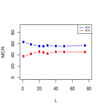
(a) $n_{1}=50$, $n_{2}=10$

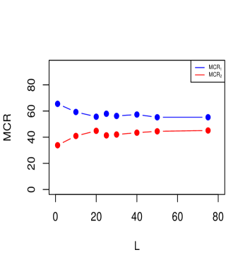
(b) $n_{1}=100$, $n_{2}=10$

Figure 2: Effect of the number of sample-splits $\mathcal{L}$ on Msplit-hr performance for the Simulation setting (iv) and $p=500$.

The following lemma shows that the variable screening method used to obtain the selection sets ${\cal S}^{(1)}_{n,t}$ have a so-called strong screening consistency property, as discussed in Pan et al. (2016). We then establish the asymptotic optimality of $\delta^{\text{Msplit-{\sc hr}}}$ in Theorem 3.2.

Lemma 3.2

Let $\mbox{\boldmath$\beta$}=\mbox{\boldmath$\Sigma$}^{-1}\mbox{\boldmath$\mu$}_{d}$, and define the active set $\mathcal{S}=\{1\leq j\leq p:\beta_{j}\neq 0\}$ with its cardinality denoted by $|\mathcal{S}|$. Furthermore, let $d_{0,n}=\min_{j\in\mathcal{S}}|\mu_{dj}|$ and $m_{max}=c_{1}(\max_{j\in\mathcal{S}}\beta_{j}^{2})|\mathcal{S}|/d_{0,n}^{2}$, for some constant $c_{1}>0$ such that $m_{max}\geq|\mathcal{S}|$. Under Condition (C2) in Appendix A, if $\tau_{n}\asymp d_{0,n}$, $\log p=o(n_{2}d_{0,n}^{2})$, $n_{2}=o(n_{1})$, and $\sqrt{n_{2}}d_{0,n}\to\infty$, as $n_{1},n_{2}\to\infty$, for any $\ell=1,...,\mathcal{L}$, we have that

$$\text{(a)}~{}\Pr\bigg{(}\mathcal{S}^{(1)}_{n,\ell}\supset\mathcal{S}\bigg{)}\to 1~{}~{};~{}~{}\text{(b)}~{}\Pr\bigg{(}|\mathcal{S}^{(1)}_{n,\ell}|\leq m_{max}\bigg{)}\to 1.$$

Part (a) implies that that for large sample sizes $n$, with probability tending to one, all the active features will be included in the selection sets $\mathcal{S}_{n,\ell}^{(1)}$, for each $\ell=1,2,\ldots,\mathcal{L}$. Part (b) shows that the size of each set $\mathcal{S}_{n,\ell}^{(1)}$ is of order $m_{max}$. These properties are obtained under the conditions that the divergence rate of the dimension $p$ is lower than that of the minority class size $n_{2}$.

Theorem 3.2

Suppose that the conditions of Lemma 3.2 are satisfied.
Let $\kappa^{\prime}_{n}=\max\{\Delta_{p}^{-1}\sqrt{m_{max}/n_{2}}~{},~{}m_{max}\sqrt{\log p/n_{1}}\}$. If $m_{max}\sqrt{\log p/n_{1}}=o(1)$, then for any fixed $\mathcal{L}$,

• the MCRs of Msplit-hr are given by

  $$\Pi_{k}^{\text{Msplit-{\sc hr}}}(\mathcal{D}_{n})=\Phi\bigg{(}-\frac{1}{2}\Delta_{p}(1+O_{p}(\kappa^{\prime}_{n}))\bigg{)},~{}~{}k=1,2$$

• if $\Delta_{p}^{2}m_{max}=o(n_{2})$ and $\Delta_{p}^{2}m_{max}\sqrt{\log p/n_{1}}=o(1)$, then the Msplit-hr is asymptotically-strong optimal.

Condition $\Delta_{p}^{2}m_{max}=o(n_{2})$ in the above theorem implies that the maximum size of the selection sets $\mathcal{S}_{n,\ell}$, that is $m_{max}$, is affected by the minority class size $n_{2}$. Note that the results of the theorem also holds for the pairwise sure independence screening of Pan et al. (2016) in the imbalanced binary cases, as well as in the balanced cases which was not studied before.

4 Two existing high-dimensional variants of LDA

In this section, we investigate conditions under which two well-known sparse variants of the LDA obtain certain optimality properties under the imbalanced setting.

4.1 Sparse LDA (slda)

This method, proposed by Shao et al. (2011), uses thresholding-type estimators for both the mean-difference vector $\mbox{\boldmath$\mu$}_{d}=\mbox{\boldmath$\mu$}_{2}-\mbox{\boldmath$\mu$}_{1}$ and $\Sigma$. In slda, a new feature vector $\textbf{x}^{*}$ is allocated to Class 1 if and only if

$$\delta^{\text{\sc slda}}(\textbf{x}^{*};\widehat{\boldsymbol{\theta}}_{n})=\tilde{\mbox{\boldmath$\mu$}}_{d}^{\top}\widetilde{\mbox{\boldmath$\Sigma$}}_{n}^{-1}(\textbf{x}^{*}-\widehat{\mbox{\boldmath$\mu$}}_{a})<0,$$

where $\widehat{\boldsymbol{\mu}}_{a}=(\widehat{\boldsymbol{\mu}}_{1}+\widehat{\boldsymbol{\mu}}_{2})/2$, and $(\widetilde{\mbox{\boldmath$\Sigma$}}_{n},\tilde{\mbox{\boldmath$\mu$}}_{d})$ are thresholded estimates of $\Sigma$ and $\mbox{\boldmath$\mu$}_{d}$, respectively, with the entries,

$$\tilde{\sigma}_{ij} = (1-2/n)~{}\widehat{\sigma}_{ij}~{}\textbf{1}\{(1-2/n)|\widehat{\sigma}_{ij}|>t_{n}\},~{}i,j=1,\ldots,p$$

$$\tilde{\mu}_{dj} = \widehat{\mu}_{dj}~{}\textbf{1}\{|\widehat{\mu}_{dj}|>a_{n}\},~{}j=1,\ldots,p,$$

where $\widehat{\sigma}_{ij}$ is $(i,j)$-th element of $\widehat{\mbox{\boldmath$\Sigma$}}_{n}$ in (2.5), and $\widehat{\mu}_{dj}$ is the $j$-th entry of $\widehat{\boldsymbol{\mu}}_{d}$ in (2.4). Further, $t_{n}=M_{1}\sqrt{\log p/n}$ with $M_{1}>0$, and $a_{n}=M_{2}(\log p/n)^{\alpha}$, $0<\alpha<1/2,M_{2}>0$.

Shao et al. (2011) derived conditions under which the slda is optimal according to their Definition 1, when $p/n\to\infty$ and $n_{1}/n\rightarrow\pi$ with $0<\pi<1$, as $n\rightarrow\infty$. It turns out that their conditions do not yield an optimal slda in the imbalanced case. In Theorem 4.1 below, we investigate conditions under which the slda is asymptotically-strong optimal under the imbalanced case. We then discuss and compare these conditions with those of Shao et al. (2011) under the balanced case.

First, for ease of comparison, we recall some notations introduced in Shao et al. (2011). Let $\widehat{q}_{n}$ be the number of features for which the value $|\widehat{\mu}_{dj}|$ is greater than $a_{n}$. Further, let $q_{n0}$ and $q_{n}$ be the number of features for which the value of $|\mu_{dj}|$ is greater than $ra_{n}$ and $a_{n}/r$, respectively, for some fixed constant $r>1$. Also let $D_{g,p}=\sum_{j=1}^{p}\mu_{dj}^{2g}$, $0\leq g<1$, and $C_{h,p}=\max_{1\leq i\leq p}\sum_{j=1}^{p}|\sigma_{ij}|^{h}$, $0\leq h<1$, be the sparsity measures corresponding to $\mbox{\boldmath$\mu$}_{d}$ and $\Sigma$, respectively. Here, $0^{0}$ is defined to be $0$. Furthermore, let $d_{n_{1}}=C_{h,p}({n_{1}}^{-1}\log p)^{(1-h)/2}$, and

$$b_{n_{1}}=\Delta_{p}^{-1}\max\left\{\Delta_{p}d_{n_{1}},~{}\sqrt{a_{n}^{2(1-g)}D_{g,p}},~{}\sqrt{q_{n}/n_{2}},~{}\sqrt{C_{h,p}q_{n}/n_{1}}\right\},$$

$$b_{n_{2}}=\Delta_{p}^{-1}\max\left\{\Delta_{p}d_{n_{1}},~{}\sqrt{a_{n}^{2(1-g)}D_{g,p}},~{}\sqrt{C_{h,p}q_{n}/n_{2}}\right\},$$

where $\Delta_{p}^{2}=\mbox{\boldmath$\mu$}_{d}^{\top}\mbox{\boldmath$\Sigma$}^{-1}\mbox{\boldmath$\mu$}_{d}$. Note that under the imbalanced setting $n_{2}=o(n_{1})$, we have $d_{n_{1}}\sim d_{n}$, where $d_{n}=C_{h,p}(n^{-1}\log p)^{(1-h)/2}$.

The following Lemma shows that the set $\{1\leq j\leq p:|\widehat{\mu}_{dj}|>a_{n}\}$ has indeed a sure screening property, which is essential in Theorem 4.1 for the assessment of slda.

Lemma 4.1

Suppose that,

$$(\log p)\left(n_{1}/\log p\right)^{2\alpha}=o(n_{2}),$$ (4.1)

and $n_{2}=o(n_{1})$, then as $n_{1},n_{2}\to\infty$,

$(a)\ \Pr\bigg{(}\bigcap_{j:|\mu_{dj}|>ra_{n}}\left\{|\widehat{\mu}_{dj}|>a_{n}\right\}\bigg{)}\to 1,\\ (b)\ \Pr\bigg{(}\bigcap_{j:|\mu_{dj}|\leq a_{n}/r}\left\{|\widehat{\mu}_{dj}|\leq a_{n}\right\}\bigg{)}\to 1,\\ (c)\ \Pr\bigg{(}q_{n0}\leq\widehat{q}_{n}\leq q_{n}\bigg{)}\to 1.$

Condition (4.1) replaces the condition $\log p/n=o(1)$ in Shao et al. (2011). One implication of (4.1) is $\log p/n_{2}=o(1)$, which shows the impact of the minority class size $n_{2}$ on the dimension allowance $p$.

Theorem 4.1

Suppose that the conditions of Lemma 4.1, and Conditions (C2) and (C3) in Appendix A are satisfied. Then, as $n_{1},n_{2}\to\infty$,

• the MCRs of slda are given by

  $$\Pi_{k}^{\text{\sc slda}}(\mathcal{D}_{n})=\Phi\bigg{(}-\frac{1}{2}\Delta_{p}\left\{1+O_{p}(b_{n_{k}})\right\}\bigg{)},~{}~{}k=1,2.$$

• the slda is asymptotically-strong optimal if

  i. $\Delta_{p}^{2}$ is bounded, and $b_{n_{2}}=o(1)$, or

  ii. $\Delta_{p}^{2}\rightarrow\infty$, such that $\Delta_{p}^{2}b_{n_{2}}=o(1)$ holds.

The difference between the above theorem and Theorem 3 of Shao et al. (2011) appears in $b_{n_{2}}$. To simplify the comparison in this case as in Shao et al. (2011), suppose that $\Sigma$ is a diagonal matrix ($C_{0,p}=1$), and let $s$ be the number of nonzero (active) entries of the mean difference vector $\mbox{\boldmath$\mu$}_{d}$. If there are two constant $c_{1},c_{2}>0$, such that $c_{1}\leq|\mu_{dj}|\leq c_{2}$, for the active $j$’s, then we have $q_{n}=s$. This implies that, by the Conditions (C2) and (C3), $\Delta_{p}^{2}$ and $D_{0,p}$ are of order $s$. Now, in this case, if $s\to\infty$, according to Theorem 4.1-(b)-ii above, under condition (4.1), $\Delta_{p}^{2}b_{n_{2}}=o(1)$ is equivalent to $s=o((n_{1}/\log p)^{\alpha})$. This implies that under the imbalanced setting, the growth rate of the sparsity factor $s$ is smaller than $\sqrt{n_{2}}$ and consequently is smaller than the growth rate of $s$ in the balanced setting. Therefore, due to the data scarcity in the minority class ($n_{2}$) in the imbalanced setting, in order for the slda to be asymptotically-strong optimal more restrictive conditions are required on both the dimension $p$ and the sparsity size $s$ compared to the balanced case.

Next, we compare the optimality conditions of Msplit-hr and slda. The relation between these conditions for a general $\Sigma$ is not straightforward, and thus to get some insight we consider a diagonal case. Suppose that $\Sigma$ is diagonal ($C_{0,p}=1$), and $g=0$ such that $D_{0,p}=s=|\mathcal{S}|$, where $\mathcal{S}=\{1\leq j\leq p:~{}\mu_{dj}\neq 0\}$. By condition (4.1), we have $\log p=o(n_{2})$ which implies the necessary conditions of Lemma 3.1 on ($s,p$), if $d_{0,n}=\min_{j\in\mathcal{S}}|\mu_{dj}|=d_{0}>0$ and $\tau_{n}=M\sqrt{n_{2}}$, for some constant $M>0$. On the other hand, if $d_{0,n}$ decays, the same conclusion holds when $a_{n}=O(d_{0,n})$ and $\tau_{n}=M\sqrt{n_{2}}d_{0,n}$. Furthermore, by (4.1) the conditions of Theorem 4.1-(b) are equivalent to $s\Delta_{p}^{2}(\log p/n_{1})^{2\alpha}=o(1)$ implying $s\Delta_{p}^{2}=o(n_{2})$ which is required for the optimality of Msplit-hr. Therefore, the conditions of Theorem 4.1 for slda on the dimension $p$ and the sparsity size $s$ are more restrictive than those in Theorem 3.1 for Msplit-hr. In terms of feature selection, Lemma 3.2-(b) provides an upper bound $m_{max}=o(n_{2}\Delta_{p}^{-2})$ on the size of the set of selected features by Msplit-hr, whereas the slda allows the number of nonzero estimators of $\mu_{dj}$’s or $\sigma_{l,j}$’s to be much larger than the class sizes to ensure optimality of the classifier, see Shao et al. (2011). Therefore, the number of selected features by slda could be potentially larger than the class sizes which we have also observed in our numerical study in Section 5.

4.2 Regularized optimal Affine discriminant (road)

This method, proposed by Fan et al. (2012), is constructed based on a sparse estimate of $\textbf{w}=\mbox{\boldmath$\Sigma$}^{-1}\mbox{\boldmath$\mu$}_{d}$, unlike the slda which uses sparse estimates of $\mbox{\boldmath$\mu$}_{d}$ and $\Sigma$, separately. The road assigns $\textbf{x}^{*}$ to Class 1 if and only if

$$\delta^{\text{\sc road}}(\textbf{x}^{*};\widehat{\boldsymbol{\theta}}_{n},c)=\widehat{\textbf{w}}_{c}^{\top}(\textbf{x}^{*}-\widehat{\boldsymbol{\mu}}_{a})<0,$$ (4.2)

where $\widehat{\boldsymbol{\theta}}_{n}=(\widehat{\boldsymbol{\mu}}_{1},\widehat{\boldsymbol{\mu}}_{2},\widehat{\mbox{\boldmath$\Sigma$}}_{n})$, $\widehat{\boldsymbol{\mu}}_{a}=(\widehat{\boldsymbol{\mu}}_{1}+\widehat{\boldsymbol{\mu}}_{2})/2$, and

$$\widehat{\textbf{w}}_{c}\in arg\min_{\|\textbf{w}\|_{1}\leq c,\ \textbf{w}^{\top}\widehat{\boldsymbol{\mu}}_{d}=1}\textbf{w}^{\top}\widehat{\mbox{\boldmath$\Sigma$}}_{n}\textbf{w}$$ (4.3)

with $\widehat{\boldsymbol{\mu}}_{d}=\widehat{\boldsymbol{\mu}}_{2}-\widehat{\boldsymbol{\mu}}_{1}$, and $(\widehat{\boldsymbol{\mu}}_{k},\widehat{\mbox{\boldmath$\Sigma$}}_{n})$ are the estimates in (2.4)-(2.5). Note that in (4.3) the smaller the $c$, the sparser the solution $\widehat{\textbf{w}}_{c}$, and as $c\to\infty$ the solution is equivalent to the regular weight $\textbf{w}_{c}\propto\mbox{\boldmath$\Sigma$}^{-1}\mbox{\boldmath$\mu$}_{d}$. Fan et al. (2012) studied the asymptotic difference between the average MCR of the road and its oracle version for which the true values of $(\mbox{\boldmath$\mu$}_{1},\mbox{\boldmath$\mu$}_{2},\mbox{\boldmath$\Sigma$})$ are used in (4.3). However, as discussed in Section 2.2, under the imbalanced setting the average MCR is not an appropriate performance measure for a classifier. Therefore, in the following theorem, we study the class-wise MCRs of the road.

Theorem 4.2

Let $s_{c}=\|\textbf{w}_{c}\|_{0}$, $s_{c}^{(1)}=\|\textbf{w}_{c}^{(1)}\|_{0}$ and $\widehat{s}_{c}=\|\widehat{\textbf{w}}_{c}\|_{0}$, where $\textbf{w}_{c}$, $\textbf{w}_{c}^{(1)}$, and $\widehat{\textbf{w}}_{c}$ are respectively the solutions of (4.3) when $(\mbox{\boldmath$\mu$}_{d},\mbox{\boldmath$\Sigma$})$, $(\widehat{\boldsymbol{\mu}}_{d},\mbox{\boldmath$\Sigma$})$ and $(\widehat{\boldsymbol{\mu}}_{d},\widehat{\mbox{\boldmath$\Sigma$}}_{n})$ are used. Furthermore, let $\Pi_{k}^{\text{\sc road}}(\mathcal{D}_{n};c)$ be the MCR of Class $k=1,2$, associated with road, and $\Pi_{k}^{\text{orc}}(c)$ denotes its oracle value. Under Condition (C2) in Appendix A, if $n_{2}=o(n_{1})$ and $\log p=o(n_{2})$, then as $n_{1},n_{2}\to\infty$,

$$\Pi_{k}^{\text{\sc road}}(\mathcal{D}_{n};c)-\Pi_{k}^{\text{orc}}(c)=O_{p}(e_{n}),\ ~{}k=1,2,$$ (4.4)

where $e_{n}=\max\bigg{\{}c^{2}(\log p)/n_{1}~{},~{}\sqrt{(\log p)/n_{2}}\times\sqrt{\max\{s_{c},\ s_{c}^{(1)},\ \widehat{s}_{c}\}}\bigg{\}}$.

By Theorem 4.2, a necessary condition for convergency of the MCRs of road to their oracle values is that the sparsity size $s_{c}$ of the vector $\textbf{w}_{c}$ and the dimension $p$ are controlled by the minority class size $n_{2}$ (similar to the slda), which in turn shows the effect of imbalanced class sizes on the performance of road.

In general, the conditions of Theorem 4.2 do not guarantee the optimality of road according to Definition 1. Fan et al. (2012) showed that when the penalty parameter $c$ is chosen as $c\geq\Delta_{p}^{-2}\parallel\mbox{\boldmath$\Sigma$}^{-1}\mbox{\boldmath$\mu$}_{d}\parallel_{1}$, then $\textbf{w}_{c}\propto\mbox{\boldmath$\Sigma$}^{-1}\mbox{\boldmath$\mu$}_{d}$ and the oracle MCRs $\Pi_{k}^{orc}(c)$ reduce to those of the optimal rule in (2.2). Hence, by Definition 1, for such $c$’s, Theorem 4.2 shows that road is asymptotically-strong sub-optimal as long as $e_{n}\to 0$. Furthermore, road becomes asymptotically-strong optimal if $\Delta_{p}$ is bounded. The condition $e_{n}\to 0$ is the same as $\log p=o(n_{1}/c^{2})$ and $\log p=o(n_{2}/s_{max})$, where $s_{max}=\max\{s_{c},\ s_{c}^{(1)},\ \widehat{s}_{c}\}$. Note that, the larger the $c$, the larger the quantities $s_{c}$, $\widehat{s}_{c}$ and $s_{c}^{(1)}$, and hence more restrictions on $(n_{1},n_{2},p)$ compared to those in Theorem 4.2, and the conditions of Msplit-hr. In our numerical study, we observe that the performance of road in terms of MCR₂ improves for lower dimensions.

5 Simulation Study

In this section, we assess the finite-sample performance of Msplit-hr and several binary classification methods using simulations. We consider two settings of diagonal and general covariance matrix $\Sigma$ under the model $\textbf{X}|Y=k\sim N_{p}(\mbox{\boldmath$\mu$}_{k},\mbox{\boldmath$\Sigma$})$, $k=1,2$.

5.1 Diagonal $\Sigma$

We compare the following methods: the bias adjusted independence (bai) and leave-one-out independence rules (loui) Bak and Jensen (2016), diagonal road method (droad) Fan et al. (2012), the bias corrected LDA (blda) Huang et al. (2010), the hr and its under-sampling version (us-hr), and our proposed method Msplit-hr. Note that the aforementioned methods use the knowledge of a diagonal $\Sigma$. In our comparison, we also include a bias-corrected support vector machines proposed by (Nakayama et al., 2017) coupled with an under-sampling method (us-bcsvm). In regards to over-sampling techniques such as the somte, Bak and Jensen (2016) and Blagus and Lusa (2013) showed that such techniques deduce larger differences between the MCRs in high-dimensional imbalanced problems. For example, we examined the performance of hr and bcsvm coupled with smote (under both diagonal and general $\Sigma$) and since their performances were not satisfactory, we did not report the results here.

We implemented the methods using R software. The droad results are based on the authors’ MATLAB codes available on their website . Our computations are carried out on a computer with an AMD Opteron(tm) Processor 6174 CPU 2.2GHz.

The above methods involve certain tuning (threshold) parameters that need to be chosen using data-driven methods. We chose best threshold parameters in blda, bai and loui by a grid search using the techniques outlined by the authors. As in Huang et al. (2010), an F-statistic is used to select the important features in blda method. In both hr and Msplit-hr, we choose the tuning parameter $\tau$ by minimizing MCR of the minority class based on a leave-one-out cross validation.

We consider the binary classification problem $\textbf{X}|(Y=k)\sim N_{p}(\mbox{\boldmath$\mu$}_{k},\textbf{D}),k=1,2$, and $\textbf{D}=\text{diag}\{\sigma_{1}^{2},...,\sigma_{p}^{2}\}$. We generated training data with different class sizes $n_{1}$ and $n_{2}$, and test data sets of size $50$ in both classes. We considered two dimensions $p=1000,3000$, and class-wise sample sizes $(n_{1},n_{2})=(25,5)$, $(50,10)$, $(100,10)$ for the training data. The simulation results are based on $100$ randomly generated data sets, and the two parameter settings:

• $\mbox{\boldmath$\mu$}_{1}=(1,1,\textbf{0}_{p-2})^{\top}$, $\mbox{\boldmath$\mu$}_{2}=(2,2.2,\textbf{0}_{p-2})^{\top}$, $\sigma_{1}^{2}=1.5^{2}$, $\sigma_{2}^{2}=0.75^{2}$, and $\sigma_{j}^{2}=1$, for $j=3,...,p$.

• $\mbox{\boldmath$\mu$}_{1}=(\textbf{1}_{9},\textbf{0}_{p-9})^{\top}$, $\mbox{\boldmath$\mu$}_{2}=(2*\textbf{1}_{4},2.5*\textbf{1}_{3},3*\textbf{1}_{2},\textbf{0}_{p-9})^{\top}$, $\sigma_{j}^{2}=10$, for $j=1,...,4$, $\sigma_{j}^{2}=2.25^{2}$, for $j=5,6,7$, $\sigma_{j}^{2}=1.5^{2}$, $j=8,9$, and $\sigma_{j}^{2}=1$, for $j=10,...,p$.

The number ($s$) of active features $x_{j}$’s that distinguish the two classes, and also the value of $\Delta_{p}$ in the two settings are respectively $s=2,\Delta_{p}^{2}=3$ and $s=9,\Delta_{p}^{2}=8.7$. Since the signal strength is measured by $\Delta_{p}$, setting (i) has a weaker signal than (ii). Under these settings, the value of the optimal MCR, $\Pi^{\text{opt}}$ in (2.2), are respectively $19.32\%$ and $7\%$. Also, the active features have different marginal signal values $|\mu_{dj}|/\sigma_{j}$, in each of the settings.

The performance measures used to compare different methods are: per-class misclassification rates (MCR₁, MCR₂), and the geometric mean ($GM$) of the MCRs. The results reported in the tables are average and standard deviations (in parentheses) of the measures over $100$ generated samples. We also reported median number of true selected features, denoted by $A$, and falsely selected features denoted by $N$, respectively. For the new method Msplit-hr, similar to the stability selection technique of Meinshausen and Bühlmann (2010), the selected features for each simulated sample are those with a relative frequency more than $50\%$, that is the set $\mathcal{S}_{n}=\{j:\frac{f_{j}}{\mathcal{L}}\geq 0.5\}$, where $f_{j}$ is selection frequency of $j$-th feature among $\mathcal{L}$ splits.

5.1.1 Discussion of the results

The results for the cases $(n_{1},n_{2},p)=$$(25,5,1000)$, $(50,10,1000)$ and $(100,10,1000)$ are given in Table 1. The results corresponding to dimension $p=3000$ are given in Table 2.

From Table 1, under both settings (i) and (ii), we can see that droad, hr, and blda have smaller error rates in the majority class (MCR₁) compared to the other methods, but the differences between their MCR₁ and MCR₂ are larger. The class-wise error rates corresponding to us-hr and us-bcsvm have smaller differences than those of droad, hr, and blda. Furthermore, the us-hr outperforms us-bcsvm, droad, hr, and blda in terms of MCR₂. Under setting (i), Msplit-hr outperforms all the other methods in terms of MCR₂; for example, its MCR₂ is better than the next best method loui up to about $8\%$, depending on class sizes $(n_{1},n_{2})$ and dimension $p$, while having balanced results for both classes. In setting (ii), Msplit-hr behaves similarly to loui and bai, with its MCR₂ better than loui and bai respectively up to about $3\%$ and $7\%$. Note that in (i), we have a weaker signal strength ($\Delta_{p}^{2}$) and fewer number of active features ($s$) than (ii), which matches the conditions of Theorem 3.1 for Msplit-hr on controlling the size of $s\Delta_{p}^{2}$. In other words, we can see that the weaker the signal, the better the performance of Msplit-hr in terms of MCRs in both classes. On the other hand, from the columns $A$ and $N$ of Table 1, Msplit-hr tends to select fewer number of inactive (noise) features compared to the two its competitors bai and loui. In bcsvm, the bias caused by dimension is corrected by using all features in the model and therefore this method does not perform any feature selection.

Table 1: Classification results for the simulation settings (i)-(ii) with a diagonal $\Sigma$ and $p=1000$.

$(n_{1},n_{2})$	Setting	Methods	$MCR_{1}\%$	$MCR_{2}\%$	$GM\%$	$A$	$N$
(25,5)	(i)	us-bcsvm	48.96(13.99)	47.46(14.38)	46.33(5.99)	2	998
		DROAD	2.62(7.45)	93.14(15.91)	5.45(11.37)	2	364
		HR	15.96(13.02)	67.3(26.43)	26.25(15.45)	1	2
		US-HR	44.34(16.45)	45.14(16.49)	42.73(8.91)	1	143.5
		BLDA	14.72(11.05)	70.16(22.47)	28.04(11.75)	1	5
		BAI	38.86(15.16)	48.2(17.23)	41.15(10.06)	1	75.5
		LOUI	41.46(18.14)	43.9(19.43)	39.05(11.75)	1	20.5
		Msplit-HR	42.66(16.97)	40.04(16.65)	39.12(11.01)	1	2
(25,5)	(ii)	us-bcsvm	46.42(14.04)	41.22(12.27)	41.99(5.75)	9	991
		DROAD	5.46(8.63)	58.48(30.27)	9.84(10.24)	6	17
		HR	12.38(10.52)	55.78(27.55)	20.80(12.40)	1	2
		US-HR	39.34(14.75)	35.48(15.43)	35.13(9.11)	4	124
		BLDA	11.06(8.74)	57.48(26.60)	20.85(11.30)	2	3
		BAI	30.72(13.94)	35.06(16.32)	30.53(10.12)	3	33
		LOUI	29.86(14.54)	31.24(16.37)	27.95(10.83)	3	36.5
		Msplit-HR	32.2(15.57)	28.22(15.44)	27.61(9.91)	1	3.5
(50,10)	(i)	us-bcsvm	47.88(10.19)	44.56(10.78)	45.25(5.71)	2	998
		DROAD	6.30(9.10)	75.28(30.25)	11.23(11.61)	2	68
		HR	19.36(7.47)	40.82 (20.99)	26.15(7.68)	1	1
		US-HR	34.22(14.05)	32.66(14.34)	32.12(10.72)	1	0
		BLDA	18.26(8.82)	48.68(21.24)	25.27(8.81)	1	3
		BAI	31.94(14.39)	36.92(15.19)	32.71(10.52)	1	11
		LOUI	29.28(12.21)	34.12(17.04)	29.99(10.39)	1	8.5
		Msplit-HR	30.22(12.66)	26.68(13.42)	26.99(9.75)	1	0
(50,10)	(ii)	us-bcsvm	41.72(9.03)	38.02(10.21)	38.93(5.23)	9	991
		DROAD	5.60(6.04)	30.72(19.67)	9.39(6.22)	7	17.5
		HR	11.02(7.04)	25.42(15.69)	14.59(6.84)	2	0
		US-HR	22.84(10.14)	19.04(8.49)	19.74(7.23)	1	0
		BLDA	11.72(6.70)	24.36(15.71)	14.80(6.13)	2	0
		BAI	17.6(8.76)	19.8(11.79)	17.18(8.07)	3	3
		LOUI	16.72(8.55)	19.16(10.99)	16.55(7.39)	3	3.5
		Msplit-HR	19.22(9.58)	17.82(9.07)	17.08(6.84)	2	0
(100,10)	(i)	us-bcsvm	47.96(10.08)	44.1(10.50)	45.09(5.42)	2	998
		DROAD	2.60(5.25)	85.74(22.67)	6.28(9.67)	2	494
		HR	19.96(8.53)	34.82(19.40)	24.31(8.09)	1	0
		US-HR	34.08(13.17)	30.52(13.07)	31.14(9.29)	1	0
		BLDA	16.84(7.60)	45.48(22.81)	25.08(8.01)	1	2
		BAI	28.86(12.15)	33.64(16.62)	29.72(9.85)	1	7
		LOUI	26.26(11.03)	32.48(16.76)	27.81(9.26)	1	6
		Msplit-HR	27.94(12.09)	24.84(13.11)	24.95(8.93)	1	0
(100,10)	(ii)	us-bcsvm	41.66(9.67)	37.38(10.88)	38.51(6.02)	9	991
		DROAD	3.22(4.23)	37.96(20.38)	6.57(6.07)	8	31.5
		HR	10.02(6.20)	22.14(12.49)	13.11(5.77)	3	0
		US-HR	20.64(10.65)	18.98(10.47)	18.30(7.76)	1	0
		BLDA	10.44(6.26)	22.28(14.29)	12.96(5.83)	3	0
		BAI	16.44(9.70)	17.08(10.19)	15.49(7.89)	3.5	2
		LOUI	15.02(8.37)	15.94(9.32)	14.13(6.42)	3	2
		Msplit-HR	16.56(8.98)	14.38(7.88)	14.04(5.36)	3	0

Table 2: Classification results for Simulation settings (i)-(ii) with a diagonal $\Sigma$ and $p=3000$.

$(n_{1},n_{2})$	Setting	Methods	$MCR_{1}\%$	$MCR_{2}\%$	$GM\%$	$A$	$N$
(25,5)	(i)	us-bcsvm	50.84(13.78)	47.32(13.75)	47.32(5.03)	2	2998
		DROAD	3.14(7.66)	94.40(12.91)	6.71(13.44)	1	529
		HR	14.92(12.68)	73.64(24.84)	26.10(16.85)	0	1.5
		US-HR	46.38(16.21)	46.86(16.10)	44.25(7.23)	1	255
		BLDA	13.6(11.63)	76.44(23.64)	26.03(14.53)	1	5
		BAI	38.04(15.86)	50.92(17.61)	41.77(9.48)	1	107.5
		LOUI	41.02(18.00)	47.04(18.60)	41.16(10.20)	1	42
		Msplit-HR	43.06(19.61)	44.08(19.25)	40.09(9.18)	1	3
(25,5)	(ii)	us-bcsvm	47.12(13.88)	45.32(13.29)	44.37(5.11)	9	2991
		DROAD	5.54(8.59)	60.58(28.94)	10.24(11.52)	6	16
		HR	14.04(12.40)	62.44(27.65)	23.41(14.78)	1	1
		US-HR	43.78(15.90)	41.52(15.33)	40.35(8.22)	3	251.5
		BLDA	11.04(10.41)	65.64(27.20)	20.50(13.70)	1	3
		BAI	33.04(15.35)	41.68(17.60)	34.84(10.61)	3	79.5
		LOUI	31.64(16.28)	41.84(18.91)	33.63(10.90)	3	78
		Msplit-HR	37.78(17.62)	36.32(17.68)	34.18(10.36)	1	3
(50,10)	(i)	us-bcsvm	48.46(11.56)	47.98(11.55)	47.04(5.29)	2	998
		DROAD	5.7(9.27)	81.02 (24.78)	11.01(13.54)	2	77
		HR	18.68(8.29)	40.88 (24.32)	24.61(9.61)	1	0
		US-HR	35.62(13.25)	36.66(14.57)	34.87(10.01)	1	0
		BLDA	17.16(8.35)	48.18(24.08)	25.74(8.52)	1	2
		BAI	32.08(11.86)	37.42(17.28)	33.32(11.03)	1	12.5
		LOUI	31.1(12.33)	34.82(17.41)	31.48(11.18)	1	9.5
		Msplit-HR	32.3(12.81)	30.98(16.05)	30.35(11.34)	1	0
(50,10)	(ii)	us-bcsvm	44.08(10.75)	44.16(10.42)	43.04(4.85)	9	991
		DROAD	5.12(5.21)	32.40(17.42)	9.24(6.25)	1	25.50
		HR	12.98(8.14)	28.7 (18.25)	17.14(8.18)	2	0
		US-HR	26.8(12.13)	24.72(12.17)	24.48(8.81)	1	0
		BLDA	12.7(6.88)	29.1(19.32)	16.70(7.20)	2	1
		BAI	20.24(10.71)	22.44(13.68)	19.55(9.60)	3	4
		LOUI	19.02(10.22)	22.74(13.48)	19.45(9.35)	3	9
		Msplit-HR	21.4(11.07)	19.2(10.14)	18.93(7.47)	2	0
(100,10)	(i)	us-bcsvm	48.3(10.85)	48.58(11.83)	47.32(5.50)	2	998
		DROAD	1.80(4.23)	88.66(20.70)	4.49(8.31)	2	861.50
		HR	18.42(8.24)	42.38(24.65)	25.08(9.02)	1	0.50
		US-HR	36.94(14.20)	37.1(13.93)	35.91(10.47)	1	0
		BLDA	15.64(8.56)	50.18(26.11)	24.00(9.47)	1	2
		BAI	29.92(10.65)	39.64(16.46)	33.37(10.74)	1	14.5
		LOUI	27.04(10.72)	36.04(17.31)	29.95(10.71)	1	7
		Msplit-HR	31.46(11.87)	29.1(15.09)	29.14(11.13)	1	0
(100,10)	(ii)	us-bcsvm	44.52(10.96)	44.74(10.91)	43.52(5.09)	9	991
		DROAD	3.28(4.47)	38.90(20.50)	6.74(6.38)	1	31.5
		HR	10.18(6.08)	27.96(18.17)	14.07(6.17)	2	0
		US-HR	24.28(11.97)	24.48(12.20)	22.97(8.76)	1	0
		BLDA	10.06(6.06)	28.26(18.13)	14.25(6.17)	2	1
		BAI	17.32(9.01)	20.94(14.02)	17.39(8.37)	3	3
		LOUI	16.08(8.97)	21.32(13.90)	17.06(8.32)	3	3
		Msplit-HR	18.64(9.41)	18.04(11.09)	16.84(8.28)	2	0

Table 2 consists of the results for dimension $p=3000$. As expected, the class-specific MCRs of all the methods increase compared to $p=1000$. Msplit-hr outperforms all the other techniques in terms of MCR₂ while having balanced misclassification rates. For example, the MCR₂ of Msplit-hr is smaller than the next best method loui up to about $7\%$. In addition, we observe that Msplit-hr has better performance than bai and loui even in setting (ii) in which they have comparable performance for $p=1000$.

We now assess the computational efficiency of the different methods. For a fixed threshold, the computational complexity of bai and loui is $O(n^{2}p)$ and that of all the other methods is $O(np)$. In our simulations, the threshold (or tuning) parameter in each method was chosen using a cross validation criterion. Table 3 provides the average computational time (in seconds) taken by each method to complete per-sample results. Note that since us-bcsvm does not involve any feature selection step, as expected, this method is among the faster methods discussed here. It can be seen that the hr and blda, followed by us-hr and us-bcsvm, are the fastest among all the methods we considered, but they are outperformed by the other methods in terms of the error rate in the minority class. In addition, while bai and loui’s performances in terms of the error rates in the minority class are comparable to our proposed method Msplit-hr; the former are slower in terms of computational time.

Table 3: Average computational time (in seconds) taken by a method to complete per-sample results: Simulation setting (i).

$(n_{1},n_{2},p)$	us-bcsvm	DROAD	HR	US-HR	BLDA	BAI	LOUI	Msplit-HR
(25,5,1000)	2.8	21.73	0.9	4.66	1.05	6	6.39	9.27
(50,10,1000)	5.12	30.77	1.47	19.98	3.53	58	260	92
(100,10,1000)	4.76	35.00	5.43	42.22	11.20	421	365	185
(25,5,3000)	7.5	97.58	1.13	9.05	1.75	14.72	13.83	19.63
(50,10,3000)	12.38	146.17	4.40	62.54	12.24	225	219	282
(100,10,3000)	10.67	141.82	19.90	169.97	29.34	1517	2294	1200

5.2 General $\Sigma$

We considered the same binary classification problem as in Section 5.1, i.e. $\textbf{X}|(Y=k)\sim N_{p}(\mbox{\boldmath$\mu$}_{k},\mbox{\boldmath$\Sigma$}),k=1,2$, but with a general non-diagonal $\Sigma$. We generated training data with different class sizes $n_{1}$ and $n_{2}$, and test data sets of sizes $50$ in both classes. The simulation results are based on $100$ randomly generated data sets. The parameter settings are:

• $\mbox{\boldmath$\mu$}_{1}=\textbf{0}_{p}$, $\mbox{\boldmath$\mu$}_{2}^{\top}=(1,0.5*\textbf{1}_{5}^{\top},0.1*\textbf{1}_{5}^{\top},\textbf{0}_{p-11}^{\top})$, $(\mbox{\boldmath$\Sigma$})_{ij}=0.8$, for $i\neq j$, $(\mbox{\boldmath$\Sigma$})_{ii}=4$, for $i=1,...,p$ and $\Delta_{p}^{2}=0.71$.

• $\mbox{\boldmath$\mu$}_{1}=\textbf{0}_{p}$, $\mbox{\boldmath$\mu$}_{2}^{\top}=(1,\textbf{0}_{4}^{\top},0.1,\textbf{0}_{p-6}^{\top})$, $\mbox{\boldmath$\Sigma$}=\left[\begin{smallmatrix}\mbox{\boldmath$\Sigma$}_{1}&&\textbf{0}\\ &\mbox{\boldmath$\Sigma$}_{2}&\\ \textbf{0}&&\ddots\end{smallmatrix}\right]$, where $(\mbox{\boldmath$\Sigma$}_{1})_{ij}=0.3$, and $(\mbox{\boldmath$\Sigma$}_{2})_{ij}=0.8$, for $i\neq j$, $(\mbox{\boldmath$\Sigma$}_{1})_{ii}=(\mbox{\boldmath$\Sigma$}_{2})_{ii}=1$, for $i=1,...,5$ and $\Delta_{p}^{2}=1.27$.

In what follows, using the same performance measures described in Section 5.1, we compare these methods: fair, slda, road, Msplit-hr, a binary version of the pairwise sure independent screening (psis) method by Pan et al. (2016), bias adjusted road (ba-road) and leave-one-out road (lou-road) by Bak and Jensen (2016), and us-bcsvm mentioned in Section 5.1. For the fair, road, ba-road, lou-road, we used the techniques based on cross-validation described in the related papers for selecting tuning parameters. We applied the bi-section method of Li and Shao (2015) for tuning parameter selection in slda by minimizing the MCR of the minority class (called slda${}_{\text{\sc mcr}_{2}}$, in the tables).

All the aforementioned methods provide sparse estimates, say $\widehat{}\mbox{\boldmath$\beta$}$, of the vector $\mbox{\boldmath$\beta$}=(\beta_{j}:1\leq j\leq p)^{\top}=\mbox{\boldmath$\Sigma$}^{-1}\mbox{\boldmath$\mu$}_{d}$ by either plugging in particular sparse estimates of $\mbox{\boldmath$\mu$}_{d}$ and $\Sigma$, or by directly finding sparse estimate of $\beta$. Thus, in our simulation results for each method, we also report the number of $j$’s for which $\widehat{\beta}_{j}\not=0$, denoted by $S$ in the tables. For Msplit-hr, we report the cardinality of the set $\mathcal{S}_{n}=\{1\leq j\leq p:\frac{f_{j}}{\mathcal{L}}\geq 0.5\}$, where $f_{j}$ is the selection frequency corresponding to index $j$ over the splits $\ell=1,...,\mathcal{L}$. Table 4 contains the simulation results for $(n_{1},n_{2},p)=(25,5,200)$, $(50,10,200)$ and $(100,10,200)$, and the results for the dimension $p=500$ are given in the Table 5.

5.2.1 Discussion of the results

From Tables 4 and 5, under both settings (iii) and (iv), we can see that fair, slda, psis and road tend to classify more observations to the majority class, and resulting in large differences between the two MCRs. Overall, the techniques us-bcsvm, ba-road, lou-road and Msplit-hr perform better than fair, slda, psis and road in terms of MCR₂ and the geometric mean. For the setting (iii), in the case $(n_{1},n_{2})=(25,5)$, Msplit-hr outperforms others, and in the cases, $(n_{1},n_{2})=(50,10)$ and $(100,10)$, the us-bcsvm and lou-road have better performance than others; for example, when $(n_{1},n_{2})=(100,10)$, lou-road outperforms Msplit-hr about $4\%$. For the setting (iv), Msplit-hr outperforms all the other techniques in terms of MCR₂; for example outperforms bc-svm and lou-road respectively up to about $10\%$ and $12\%$ depending on the values of $(n_{1},n_{2},p)$. Moreover, this performance of Msplit-hr is based on a much smaller set of selected features compared to its competitors. In summary, Msplit-hr has better performance in the setting (iv) which includes more features with weak signals than (iii).

Table 4: Classification results for the simulation settings (iii)-(iv) with a general $\Sigma$ and $p=200$.

$(n_{1},n_{2})$	Setting	Methods	$MCR_{1}\%$	$MCR_{2}\%$	$GM\%$	$S$
(25,5)	(iii)	us-bcsvm	46.26(15.97)	51.22(15.50)	46.20(6.30)	200
		FAIR	23.22(9.64)	78.56(10.26)	40.53(8.04)	6.87
		SLDA${}_{\text{\sc mcr}_{2}}$	42.04(14.38)	57.38(14.87)	47.02(6.55)	147.07
		PSIS	31.56(9.44)	66.98(10.51)	45.02(6.21)	1
		ROAD	15.47(8.03)	82.67(8.87)	34.16(6.89)	26.17
		BA-ROAD	48.20 (12.51)	48.91(12.36)	46.83(4.55)	56.45
		LOU-ROAD	48.07(12.27)	49.03(12.40)	46.97(2.55)	54.09
		Msplit-HR	53.58(15.06)	45.76(16.23)	47.12(6.65)	4
(25,5)	(iv)	us-bcsvm	49.96(15.76)	46(15.44)	45.39(5.62)	200
		FAIR	20.96(8.00)	76.38(10.82)	38.83(6.85)	8.07
		SLDA${}_{\text{\sc mcr}_{2}}$	37.18(14.30)	60.74(14.84)	45.31(7.84)	124.39
		PSIS	30.02(9.15)	62.52(16.16)	42.17(8.64)	1
		ROAD	15.77(7.24)	78.93(11.66)	33.94(6.09)	24.38
		BA-ROAD	46.52(15.06)	46.63(16.65)	43.92(7.17)	48.53
		LOU-ROAD	46.34(15.79)	46.22(17.97)	43.17(7.63)	47.26
		Msplit-HR	52.32(18.66)	43.02(18.51)	43.77(7.92)	4.5
(50,10)	(iii)	us-bcsvm	46.34(11.67)	48.88(12.77)	46.27(5.25)	200
		FAIR	28.98(8.96)	69.1(8.95)	43.96(6.76)	6
		SLDA${}_{\text{\sc mcr}_{2}}$	44.5(11.65)	55.84(12.40)	48.57(5.37)	195
		PSIS	37.96(8.26)	60.72(8.67)	47.47(5.54)	1
		ROAD	19.98(8.79)	77.54(9.02)	38.07(7.11)	44
		BA-ROAD	48.36(14.40)	48.50(14.15)	45.99(9.29)	53.50
		LOU-ROAD	47.38(11.90)	49.14(12.19)	46.99(6.34)	53
		Msplit-HR	50.76(13.85)	47.64(12.15)	47.65(6.11)	3
(50,10)	(iv)	us-bcsvm	47.88(11.98)	48.42(12.55)	46.76(5.53)	200
		FAIR	23.98(8.65)	64.5(12.53)	38.33(7.57)	6
		SLDA${}_{\text{\sc mcr}_{2}}$	37.5(13.23)	54.58(16.77)	43.61(9.53)	189.5
		PSIS	32.16(8.79)	51.04(17.23)	39.64(9.48)	1
		ROAD	21.68(9.25)	64.44(18.71)	35.45(7.40)	19.50
		BA-ROAD	37.82(13.06)	44.74(15.80)	39.00(10.23)	26
		LOU-ROAD	39.74(12.51)	42.46(13.50)	39.80(8.27)	27
		Msplit-HR	44.62(13.96)	40.1(14.25)	40.77(8.48)	1
(100,10)	(iii)	us-bcsvm	46.54(11.31)	48.46(12.50)	46.19(5.04)	200
		FAIR	26.08(7.63)	70.62(7.94)	42.27(6.27)	6.68
		SLDA${}_{\text{\sc mcr}_{2}}$	47.24(13.75)	54.18(12.48)	49.09(6.46)	169.26
		PSIS	36.06(8.41)	63(8.95)	46.52(6.62)	1.01
		ROAD	11.16(6.67)	86.04(8.46)	29.49(7.64)	71.70
		BA-ROAD	44.50(13.57)	50.94(13.67)	45.40(8.71)	85.41
		LOU-ROAD	44.62(10.18)	42.44(9.37)	42.79(6.12)	66.22
		Msplit-HR	50.42(15.15)	46.46(14.43)	46.22(6.99)	11.45
(100,10)	(iv)	us-bcsvm	47.76(12.15)	47.26(12.50)	46.03(5.56)	200
		FAIR	22(7.97)	67.54(11.80)	37.63(7.61)	8.03
		SLDA${}_{\text{\sc mcr}_{2}}$	34.2(11.71)	50.54(17.12)	40.03(8.67)	96.77
		PSIS	31.36(8.13)	47.58(18.24)	37.74(9.75)	1
		ROAD	11.16(6.67)	86.04(8.46)	29.49(7.64)	71.70
		BA-ROAD	44.50(13.57)	50.96(13.67)	45.39(8.71)	85.41
		LOU-ROAD	44.12(12.27)	50.54(11.72)	45.84(5.82)	97
		Msplit-HR	45.86(17.28)	37.6(14.92)	39.19(8.68)	9.25

Table 5: Classification results for the simulation settings (iii)-(iv) with a general $\Sigma$ and $p=500$.

$(n_{1},n_{2})$	Setting	Methods	$MCR_{1}\%$	$MCR_{2}\%$	$GM\%$	$S$
(25,5)	(iii)	us-bcsvm	49.18(17.81)	50.46(17.69)	46.39(8.47)	500
		FAIR	20.48(8.72)	79(8.91)	38.79(8.29)	8.91
		SLDA${}_{\text{\sc mcr}_{2}}$	44.84(15.58)	54.56(16.11)	46.97(5.57)	350.18
		PSIS	23.22(9.64)	75.68(10.26)	40.53(8.05)	6
		ROAD	12.01(8.27)	87.16(8.70)	30.21(8.08)	30.79
		BA-ROAD	44.63(13.74)	53.71(14.30)	45.01(9.74)	57.49
		LOU-ROAD	45.82(12.19)	52.32(12.41)	47.40(2.84)	69.18
		Msplit-HR	55.96(16.92)	44.58(17.43)	46.77(7.11)	3
(25,5)	(iv)	us-bcsvm	48.9(15.18)	47.66(13.96)	46.17(5.45)	500
		FAIR	15.1(8.91)	84.08(8.87)	33.15(10.97)	13.38
		SLDA${}_{\text{\sc mcr}_{2}}$	41.04(15.56)	58.3(15.45)	46.52(7.29)	315.96
		PSIS	30.26(9.52)	65.9(13.01)	43.60(7.70)	1
		ROAD	12.50(8.10)	85.07(10.66)	30.67(7.51)	27.82
		BA-ROAD	48.07(13.10)	48.40(14.23)	46.20(6.71)	60.06
		LOU-ROAD	48.47(13.37)	47.48(14.94)	45.97(5.10)	59.19
		Msplit-HR	53.06(17.66)	43.16(17.54)	44.50(8.83)	2
(50,10)	(iii)	us-bcsvm	48.46(12.44)	48.64(14.25)	46.94(5.82)	500
		FAIR	26.1(8.65)	72.12(8.35)	42.48(6.57)	9
		SLDA${}_{\text{\sc mcr}_{2}}$	43.76(12.28)	55.18(11.98)	47.78(5.51)	493.5
		PSIS	35.44(8.02)	63.02(9.33)	46.67(5.37)	1
		ROAD	14.10(9.43)	83.70(11.63)	31.80(9.44)	59.50
		BA-ROAD	48.32(14.03)	49.66(12.68)	47.15(7.68)	64.50
		LOU-ROAD	48.18(13.51)	48.26(12.33)	46.71(6.01)	68
		Msplit-HR	50.06(15.67)	48.26(14.52)	46.91(5.78)	1
(50,10)	(iv)	us-bcsvm	49.04(10.87)	49.28(11.96)	48.01(5.56)	500
		FAIR	17.38(6.91)	76.14(10.84)	35.41(7.35)	13.5
		SLDA${}_{\text{\sc mcr}_{2}}$	38.58(13.19)	51.14(14.79)	42.98(9.05)	473
		PSIS	32.02(8.58)	54.56(17.60)	40.97(9.69)	1
		ROAD	15.46(9.32)	73.56(19.75)	30.97(7.64)	38.50
		BA-ROAD	42.20(13.08)	44.26(15.04)	41.40(8.97)	38
		LOU-ROAD	42.60(13.97)	43.16(14.41)	41.25(8.55)	47
		Msplit-HR	46.4(14.65)	40.7(15.10)	41.55(8.81)	1
(100,10)	(iii)	us-bcsvm	47.96(11.92)	49.98(13.98)	47.47(5.67)	500
		FAIR	23.91(8.31)	74.6(7.48)	41.28(7.55)	8.22
		SLDA${}_{\text{\sc mcr}_{2}}$	44.28(12.54)	54.34(12.45)	47.61(5.27)	403.99
		PSIS	33.32(7.73)	65.48(8.83)	46.24(5.87)	1.01
		ROAD	4.60(3.47)	94.60(4.99)	19.02(8.42)	96.49
		BA-ROAD	45.40(13.39)	51.16(14.24)	45.90(8.21)	105.05
		LOU-ROAD	46.24(8.52)	43.12(10.44)	43.99(6.11)	103.05
		Msplit-HR	51.76(14.45)	46(14.62)	46.61(6.55)	5.67
(100,10)	(iv)	us-bcsvm	48.72(11.81)	48.94(12.06)	47.65(5.53)	500
		FAIR	15.1(7.41)	79.42(9.89)	33.09(8.62)	17.18
		SLDA${}_{\text{\sc mcr}_{2}}$	36.98(12.42)	53.58(14.94)	43.12(9.01)	226.33
		PSIS	30.28(7.57)	54.96(18.29)	39.94(9.12)	1.01
		ROAD	4.64(3.47)	94.60(4.99)	19.02(8.42)	96.49
		BA-ROAD	45.40(13.39)	51.16(14.24)	45.90(8.21)	105.05
		LOU-ROAD	45.64(13.15)	49.18(12.87)	45.79(5.82)	107.80
		Msplit-HR	43.52(12.21)	44.02(14.34)	42.38(8.26)	5.74

Next, we assess the computational efficiency of different methods by studying the average computational time (in seconds) taken by each method to complete per-sample results, which are given in Table 6. We can see that psis is the fastest method followed by fair and us-bcsvm. However, as seen above, these methods do not perform well in terms of the MCRs. As mentioned before, us-bcsvm is computationally fast, since it does not involve any feature selection step. The slda is slower than the Msplit-hr when the dimension $p$ is increased from $p=200$ to $500$. On the other hand, Msplit-hr is computationally more efficient than its two competitors ba-road and lou-road. Note that, for a fixed value of tuning parameter, the computational complexity of ba-road and lou-road is $O(n^{2}p^{2})$, and that of Msplit-hr is $O(np^{2})$. Therefore, even without a tuning selection procedure, our technique has lower computational cost.

Table 6: Average computational time (in seconds) taken by a method to complete per-sample results: Simulation setting (iv).

$(n_{1},n_{2},p)$	us-bcsvm	FAIR	SLDA${}_{\text{\sc mcr}_{2}}$	PSIS	ROAD	BA-ROAD	LOU-ROAD	Msplit-HR
(25,5,200)	1.91	1.75	8.75	0.28	50.23	110.34	59.93	11.42
(50,10,200)	1.48	4.73	25.71	4.11	66.00	192.10	189.86	39.31
(100,10,200)	1.86	5.56	66.46	3.06	120.93	468.02	443.23	114.44
(25,5,500)	3.00	29.3	80.05	0.41	204.52	254.64	184.99	16.4
(50,10,500)	3.01	27.09	234.35	3.00	272.15	483.82	477.45	62.23
(100,10,500)	3.58	29.66	451.75	3.61	219.95	974.34	1084.75	176.65

In summary, given the difficulty of the imbalanced problem, our current simulation study shows that (considering all the three factors: misclassification rates, feature selection, and computational efficiency) Msplit-hr has a good performance compared to the methods discussed here, and is yet another reliable technique for high-dimensional imbalanced problems.

6 Real-data analysis

We now demonstrate the performance of different methods on two real data sets.

The first data set, on breast cancer (Gravier et al., 2010), consists of the expression profiles of $2905$ genes for $168$ patients of whom $111$ patients with no event after diagnosis were labelled as “good” and the remaining $57$ patients with early metastasis were labelled as “poor”. In our analysis, we randomly split the data into training data of sizes $56$ and $28$ of respectively good cases (the majority Class 1) and poor cases (the minority Class 2). The rest of the data is used for testing. The classification results, under the assumptions of (a) uncorrelated and (b) correlated features, are given in Table 7. Under (a), the results suggest that bai, loui, Msplit-hr, and us-hr have comparable performance, with bai and loui performing slightly better than the other two in terms of the MCR of the minority class (MCR₂). Under (b), ba-road, lou-road, and Msplit-hr perform similar in terms of the MCRs. us-bcsvm has smaller MCRs compared to the others but by using the set of all features as it is not able to perform any feature selection. Note that in both cases, Msplit-hr selects a much smaller number of features toward the classification task.

Table 7: Classification results for Breast Cancer data set. $S$ denotes the median number of selected features.

$\Sigma$	Methods	$MCR_{1}\%$	$MCR_{2}\%$	$GM\%$	$S$
Diagonal	DROAD	19.62(10.20)	46.31(13.38)	28.72(7.77)	201.50
	HR	16.82(6.70)	46.72(10.24)	27.08(5.98)	26
	US-HR	20.67(7.58)	39.79(9.78)	27.93(6.10)	32
	BLDA	16.8(6.14)	45.59(10.86)	26.78(5.63)	35
	BAI	22.24(7.09)	37(10.08)	27.83(5.40)	99
	LOUI	22.65(7.05)	37.03(10.82)	28.06(5.20)	83.5
	Msplit-HR	20.96(7.00)	39.56(10.74)	27.83(5.19)	6
General	us-bcsvm	19.78(5.74)	34.79(10.01)	25.50(4.24)	1500
	FAIR	16.24(5.54)	45.41(9.31)	26.43(4.95)	22
	SLDA${}_{\text{\sc mcr}_{2}}$	22.91(12.32)	47.76(12.19)	31.58(9.17)	1500
	PSIS	27.47(14.62)	46.17(15.30)	33.77(9.85)	1
	ROAD	19.51(10.03)	47.41(13.81)	28.96(7.26)	25
	BA-ROAD	22.16(5.95)	38.83(9.72)	28.62(4.24)	51.50
	LOU-ROAD	22.16(5.90)	38.10(9.84)	28.37(4.32)	56.50
	Msplit-HR	24.11(8.85)	40.55(10.76)	30.35(6.50)	5

Table 8: Classification results for Myeloma Cancer data set. $S$ denotes the median number of selected features.

$\Sigma$	Methods	$MCR_{1}\%$	$MCR_{2}\%$	$GM\%$	$S$
Diagonal	DROAD	26.03(11.29)	49.33(10.30)	34.93(8.58)	5
	HR	25.94(11.60)	57.78(11.92)	37.43(8.47)	19
	US-HR	41.6(9.74)	41(12.75)	40.17(6.66)	92.5
	BLDA	25.58(9.10)	53.28(11.23)	35.89(6.36)	11
	BAI	34.31(10.44)	44.17(13.20)	37.50(5.98)	30
	LOUI	35.14(10.54)	44.39(11.35)	38.26(5.95)	27.5
	Msplit-HR	38.18(13.68)	41.94(14.37)	37.89(7.51)	7
General	us-bcsvm	53.78(27.56)	39.44(28.32)	46.06(18.47)	1500
	FAIR	27.92(7.64)	49.56(11.16)	36.50(6.15)	14
	SLDA${}_{\text{\sc mcr}_{2}}$	28.83(9.79)	47.22(10.34)	36.18(7.59)	13
	PSIS	31.42(15.24)	50.11(10.33)	38.43(10.72)	1
	ROAD	26.01(10.27)	53.22(10.63)	36.47(8.13)	7.50
	BA-ROAD	34.01(13.75)	43.17(13.92)	35.52(9.38)	20
	LOU-ROAD	33.74(9.63)	42.78(10.67)	38.05(6.43)	23.50
	Msplit-HR	34.74(11.84)	42.61(11.66)	37.27(7.16)	6

The second data set, on multiple-myeloma cancer (Tian et al., 2003), consists of the expression profiles of $12,2625$ genes for $173$ patients with newly diagnosed multiple-myeloma, of whom $137$ were with bone lytic lesions and the remaining $36$ patients were without bone lytic lesions. We randomly choose a training set containing $18$ observations from patients labelled by MRI-no-lytic-lesion (the minority Class 2), and $72$ observations from patients labelled by MRI-lytic-lesion (the majority Class 1). The rest of the data were used for testing. Table 8 contains the classification results under the aforementioned assumptions (a) and (b). Under (a), the results show that Msplit-hr and us-hr outperform the other methods in terms of the error rate in the minority class, MCR₂. In addition, Msplit-hr outperforms us-hr in terms of the error rate in the majority class, MCR₁. Under (b), the three methods ba-road, lou-road, and Msplit-hr perform similar in terms of the MCRs. For this data set, the overall performances of the aforementioned three methods are better than us-bcsvm. Note that in both cases, Msplit-hr selects a smaller number of features toward the classification task.

To reduce the computational cost of each method, and by using a t-statistic, we screened the initial number of features in each of the above data sets by selecting a subset of $p=1500$ genes.

7 Conclusion

In this paper, we have studied linear discriminant analysis (LDA) in high-dimensional imbalanced binary classification. To the best of our knowledge, this is the first work that rigorously investigates such problems which frequently arise in a wide range of applications.

First, we showed that in the aforementioned settings the standard LDA asymptotically ignores the so-called minority class. Second, using a multiple data splitting technique, we proposed a new method, called Msplit-hr, that obtains desirable large-sample properties. Third, we derived conditions under which two well-known sparse versions of the LDA in our setting obtain certain desirable large-sample properties. We then examined the finite-sample performance of different methods via simulations and by analyzing two real data sets. In our simulations, the Msplit-hr either outperforms competing methods or has comparable performance in terms of misclassification rate in the minority class, while it has a lower computational cost.

The methodology (Msplit-hr) and theory developed in this paper are based on normal distribution for the feature vector X. The normality is used for bias calculations in Propositions 3.1-3.2, and to establish feature selection consistency in Lemmas 3.1-3.2. On the other hand, Delaigle and Hall (2012) showed that feature selection methods based on mean-differences are sensitive to heavy-tailed distributions for X, and they suggested transformation approaches in feature space which are more resistant to extreme observations from heavy-tailed distributions. Properties of such transformations with respect to our theoretical guidelines, and in general, extension of our results to non-normal models require further investigation and is a topic of future research.

If the covariance matrix differs between the two classes, i.e. $\textbf{X}|(Y=k)\sim N(\mbox{\boldmath$\mu$}_{k},\mbox{\boldmath$\Sigma$}_{k}),k=1,2$, the optimal (Bayes) rule is the quadratic discriminant analysis (QDA). Our limited numerical experiment shows that the QDA in imbalanced high-dimensional problems behaves similarly to the LDA ignoring the minority class. A potential approach to alleviate the impact of imbalanced class sizes is to reduce the difference between MCRs of an empirical QDA toward that of the optimal rule. However, the main challenge is that none of the aforementioned MCRs have workable closed forms. Li and Shao (2015) studied such differences for sparse QDA, and their results might be useful toward imbalanced problems in the context of QDA. This, however, requires a careful investigation and is a subject of future work.

Another possible future research direction is to investigate the possibility of extending the methodology and theory developed in this paper to imbalanced multi-class classification problems.

Appendix A Technical Lemmas

In this Appendix, we first state the technical conditions (C1)-(C3) required in our theoretical developments. Next, we state several lemmas that are used in the proofs of our main results. Lemmas A.1 and A.2 are from Bickel and Levina (2008b) and Shao et al. (2011). Lemmas A.3-A.5 are the results from other papers adapted to the imbalanced setting under our consideration. Lemma A.6 states an upper bound for the tail of Student’s t-distribution.

Technical Conditions:

• $\log p=o(n_{1})$, where $n_{1}$ is the majority class size.

• $~{}0<c_{0}^{-1}<\lambda_{min}(\mbox{\boldmath$\Sigma$})\leq\lambda_{max}(\mbox{\boldmath$\Sigma$})<c_{0}<\infty$, for a constant $c_{0}>0$.

• $~{}0<c_{0}^{-1}<\max_{j=1,...,p}\mu_{dj}^{2}<c_{0}<\infty$, where $\mbox{\boldmath$\mu$}_{d}=\mbox{\boldmath$\mu$}_{2}-\mbox{\boldmath$\mu$}_{1}$.

Lemma A.1

(Bickel and Levina, 2008b, Lemma A.3) Let $\textbf{Z}_{i}$ be independent and identically random variables from $N_{p}(\textbf{0},\mbox{\boldmath$\Sigma$})$ and $\lambda_{\max}(\mbox{\boldmath$\Sigma$})\leq\varepsilon_{0}^{-1}<\infty$. Then,

$$P\left(\mid\sum_{i=1}^{n}(Z_{ij}Z_{ik}-\sigma_{jk})\mid>n\nu\right)\leq C_{1}\exp(-C_{2}n\nu^{2})\quad\text{for all}\ |\nu|\leq\delta$$

where $\sigma_{jk}$’s are entries of $\Sigma$, and $C_{1}$, $C_{2}$, and $\delta$ depend on $\epsilon_{0}$ only.

Lemma A.2

(Shao et al., 2011, Lemma 1) Let $\xi_{n}$ and $\nu_{n}$ be two sequence of positive numbers such that $\xi_{n}\rightarrow\infty$ and $\nu_{n}\rightarrow 0$ as $n\rightarrow\infty$. If $\lim_{n\rightarrow\infty}\xi_{n}\nu_{n}=\gamma$, where $\gamma$ may be $0$, positive or $\infty$, then

$$\lim_{n\rightarrow\infty}\frac{\Phi(-\sqrt{\xi_{n}}(1-\nu_{n}))}{\Phi(-\sqrt{\xi_{n}})} = e^{\gamma}.$$

Lemma A.3

Denote the sets

$$U_{\tau}(h,c_{0}(p),M) = \bigg{\{}\mbox{\boldmath$\Sigma$}:\ \sigma_{ii}\leq M,\sum_{j=1}^{p}|\sigma_{ij}|^{h}\leq c_{0}(p),\ \forall i,\ 0\leq h<1\bigg{\}},$$

$$U_{\tau}(h,c_{0}(p),M,\epsilon_{0}) = \bigg{\{}\mbox{\boldmath$\Sigma$}:\ \mbox{\boldmath$\Sigma$}\in U_{\tau}(h,c_{0}(p),M),\lambda_{min}(\mbox{\boldmath$\Sigma$})\geq\epsilon_{0}>0\bigg{\}}.$$

Let $\widetilde{\mbox{\boldmath$\Sigma$}}_{n}$ be a thresholded version of the pooled sample covariance matrix $\widehat{\mbox{\boldmath$\Sigma$}}_{n}$ in (2.5), such that $\tilde{\sigma}_{ij}=(1-2/n)\widehat{\sigma}_{ij}\textbf{1}\{(1-2/n)|\widehat{\sigma}_{ij}|>t_{n}\}$, with $t_{n}=M_{1}\sqrt{\frac{\log p}{n}}$ and some positive constant $M_{1}$. Then uniformly on $U_{\tau}(h,c_{0}(p),M)$, and for sufficiently large $M_{1}$, under the Condition (C3) and $n_{2}=o(n_{1})$, as $n_{1},n_{2}\to\infty$, then

$$\parallel\widetilde{\mbox{\boldmath$\Sigma$}}_{n}-\mbox{\boldmath$\Sigma$}\parallel=O_{p}\bigg{(}c_{0}(p)\left(\log p/n_{1}\right)^{\frac{1-h}{2}}\bigg{)},$$

and uniformly on $U_{\tau}(h,c_{0}(p),M,\epsilon_{0})$,

$$\parallel\widetilde{\mbox{\boldmath$\Sigma$}}_{n}^{-1}-\mbox{\boldmath$\Sigma$}^{-1}\parallel=O_{p}\bigg{(}c_{0}(p)\left(\log p/n_{1}\right)^{\frac{1-h}{2}}\bigg{)}.$$

Proof. The proof is a straight forward extension of Theorem 1 of Bickel and Levina (2008a) to imbalanced case, and thus omitted here. $\blacksquare$

Lemma A.4

Let $\textbf{X}_{ik}=(X_{i1k},...,X_{ipk})^{\top}$, for $i=1,...,n_{k}$, and $k=1,2$, be random samples from $p$-variate normal distribution with mean vector $\mathrm{𝟎}$ and diagonal covariance matrix $\textbf{D}=diag\{\sigma_{1}^{2},...,\sigma_{p}^{2}\}$. If the Conditions (C1) and (C2) are satisfied and $n_{2}=o(n_{1})$, then as $n_{1},n_{2}\to\infty$, we have

$$\max_{1\leq j\leq p}\mid\widehat{\sigma}_{j}^{2}-\sigma_{j}^{2}\mid=O_{p}(\sqrt{(\log p)/n_{1}}),$$

where $\widehat{\sigma}_{j}^{2},j=1,\ldots,p$, are the diagonal elements of the pooled sample variance $\widehat{}\mbox{\boldmath$\Sigma$}_{n}$ in (2.5).

Proof. Let $\overline{X}_{jk}=\frac{1}{n_{k}}\sum_{i=1}^{n_{k}}X_{ijk}$, for $k=1,2$, $j=1,...,p$. We have,

$$\Pr\left(\max_{1\leq j\leq p}\mid\widehat{\sigma}_{j}^{2}-\sigma_{j}^{2}\mid>\eta\right)\leq\sum_{j=1}^{p}\Pr\left(\mid\widehat{\sigma}_{j}^{2}-\sigma_{j}^{2}\mid>\eta\right)$$

$$\leq \sum_{k=1}^{2}\sum_{j=1}^{p}\Pr\left(\frac{1}{\sqrt{n_{k}}}\mid\sum_{i=1}^{n_{k}}({X}_{ijk}^{2}-\sigma_{j}^{2})\mid>\frac{1}{\sqrt{n_{k}}}\frac{\eta}{4}(n_{1}+n_{2}-2)\right)$$

$$+ \sum_{k=1}^{2}\sum_{j=1}^{p}\Pr\left(\mid n_{k}\overline{X}_{jk}^{2}-\sigma_{j}^{2}\mid>\frac{\eta}{4}(n_{1}+n_{2}-2)\right)$$

$$\leq \sum_{k=1}^{2}pC_{1}\exp\bigg{\{}-C_{2}\frac{\eta^{2}}{16}\frac{(n-2)^{2}}{n_{k}}\bigg{\}}+pC_{3}\exp\bigg{\{}-C_{4}\frac{\eta^{2}}{16}(n-2)^{2}\bigg{\}}$$

for $|\eta|<\delta$, where $C_{1},C_{2},C_{3},C_{4}$, and $\delta$ are constants depending only on $c_{0}$. The last inequality follows from Lemma A.1. By taking $\eta=M\sqrt{\log p/n_{1}}$, for sufficiently large $M>0$, under the imbalanced setting and the Condition (C1), the result holds. $\blacksquare$

Lemma A.5

Under conditions of Lemma 3.2 and the imbalanced setting $n_{2}=o(n_{1})$, assume that $m_{max}\sqrt{\log p/n_{1}}=o(1)$. Then for $\ell=1,\dots,\mathcal{L}$, as long as $n_{1},n_{2}\to\infty$,

$$\parallel\widetilde{\mbox{\boldmath$\Sigma$}}_{n,\ell}-\mbox{\boldmath$\Sigma$}_{\ell}\parallel=O_{p}\bigg{(}m_{max}\sqrt{\log p/n_{1}}\bigg{)}.$$

where $\widetilde{\mbox{\boldmath$\Sigma$}}_{n,\ell}=[\widehat{\sigma}_{jj^{\prime},\ell}^{(2)}:~{}j,j^{\prime}\in\mathcal{S}_{n,\ell}^{(1)}]$ and $\mbox{\boldmath$\Sigma$}_{\ell}=[\sigma_{jj^{\prime}}:~{}j,j^{\prime}\in\mathcal{S}_{n,\ell}^{(1)}]$.

Proof. Note that if $\textbf{A}=[a_{jj^{\prime}}]$ be a symmetric $p\times p$ matrix then $\parallel\textbf{A}\parallel\leq\max_{j^{\prime}}\sum_{j=1}^{p}|a_{jj^{\prime}}|$. Thus, the result is implied by

$$\Pr\bigg{(}\max_{j\in\mathcal{S}_{n,\ell}^{(1)}}\sum_{j^{\prime}\in\mathcal{S}_{n,\ell}^{(1)}}|\widehat{\sigma}_{jj^{\prime},\ell}^{(2)}-\sigma_{jj^{\prime}}|>\eta\bigg{)}\leq\sum_{j,j^{\prime}\in\mathcal{S}_{n,\ell}^{(1)}}\Pr\bigg{(}|\widehat{\sigma}_{jj^{\prime},\ell}^{(2)}-\sigma_{jj^{\prime}}|>\frac{\eta}{m_{max}}\bigg{)}\hskip 36.135pt$$ (A.1)

where $m_{max}=c_{1}|\mathcal{S}|(\max_{j\in\mathcal{S}}\beta_{j}^{2})/d_{0,n}^{2}$. The inequality follows from part (ii) of Lemma 3.2. Let $\mbox{\boldmath$\mu$}_{k,\ell}=[\mu_{jk}:~{}j\in\mathcal{S}_{n,\ell}^{(1)}]$, $Z_{ijk,\ell}=X_{ijk,\ell}-\mu_{jk,\ell}$, and $\bar{Z}_{jk,\ell}=\sum_{i=1}^{n^{\prime}_{k}}X_{ijk,\ell}/n^{\prime}_{k}$, where $X_{ijk,\ell}\in\mathcal{D}_{n,\ell}^{(2)}$, for $i=1,...,n^{\prime}_{k}$, $j=1,...,p$, $k=1,2$, and $\ell=1,...,\mathcal{L}$, where $\textbf{X}_{ik,\ell}\sim N_{p}(\mbox{\boldmath$\mu$}_{k,\ell},\mbox{\boldmath$\Sigma$}_{\ell})$. For the first probability term in (A.1), we have

$$\Pr\bigg{(}|\widehat{\sigma}_{jj^{\prime},\ell}^{(2)}-\sigma_{jj^{\prime}}|>\frac{\eta}{m_{max}}\bigg{)}\leq$$

$$\sum_{k=1}^{2}\Pr\bigg{(}\bigg{|}\sum_{i=1}^{n^{\prime}_{k}}Z_{ijk,\ell}Z_{ij^{\prime}k,\ell}-n^{\prime}_{k}\bar{Z}_{jk,\ell}\bar{Z}_{j^{\prime}k,\ell}-(n^{\prime}_{k}-1)\sigma_{jj^{\prime}}\bigg{|}>\frac{(n^{\prime}-2)\eta}{m_{max}}\bigg{)}$$

$$\leq \sum_{k=1}^{2}\bigg{\{}\Pr\bigg{(}\bigg{|}\sum_{i=1}^{n^{\prime}_{k}}Z_{ijk,\ell}Z_{ij^{\prime}k,\ell}-n^{\prime}_{k}\sigma_{jj^{\prime}}\bigg{|}>\frac{(n^{\prime}-2)\eta}{m_{max}}\bigg{)}$$

$$+\Pr\bigg{(}|n^{\prime}_{k}\bar{Z}_{jk,\ell}\bar{Z}_{j^{\prime}k,\ell}-\sigma_{jj^{\prime}}|>\frac{(n^{\prime}-2)\eta}{m_{max}}\bigg{)}\bigg{\}}.$$

Finally, using Lemma A.1,

$$\sum_{j,j^{\prime}\in\mathcal{S}_{n,t}^{(2)}}\Pr\bigg{(}|\widehat{\sigma}_{jj^{\prime},\ell}^{(2)}-\sigma_{jj^{\prime}}|>\frac{\eta}{m_{max}}\bigg{)}$$

$$\leq \sum_{k=1}^{2}C_{1}p^{2}\exp\bigg{\{}-C_{2}\frac{(n-2)^{2}\eta^{2}}{m_{max}^{2}n_{k}}\bigg{\}}+C^{\prime}_{1}p^{2}\exp\bigg{\{}-C^{\prime}_{2}\frac{(n-2)^{2}\eta^{2}}{m_{max}^{2}}\bigg{\}},$$

where $C_{1},C^{\prime}_{1},C_{2},C^{\prime}_{2}$ are some positive constants. If $m_{max}\sqrt{\log p/n_{1}}=o(1)$ and by taking $\eta=M\times m_{max}\sqrt{\log p/n_{1}}$, for sufficiently large $M>0$, the desired result is obtained. $\blacksquare$

Lemma A.6

Suppose that $T$ has the Student’s t-distribution with $n>1$ degrees of freedom. Then, for any large constant $\tau>0$, we have

$$\Pr(T>\tau)\leq\frac{c_{n}}{\tau}\frac{n}{n-1}\left(1+\frac{1}{n}\tau^{2}\right)^{-\frac{n-1}{2}},$$

where $c_{n}=\frac{\Gamma(\frac{n+1}{2})}{\Gamma(\frac{n}{2})\sqrt{n\pi}}$, and $\Gamma(.)$ is the gamma function.

Proof. For any $\tau>0$,

$$\Pr(T>\tau) = \int_{\tau}^{\infty}\frac{c_{n}}{(1+\frac{x^{2}}{n})^{\frac{n+1}{2}}}dx<\int_{\tau}^{\infty}\frac{x}{\tau}\frac{c_{n}}{(1+\frac{x^{2}}{n})^{\frac{n+1}{2}}}dx$$

$$= \frac{c_{n}}{\tau}\frac{n}{n-1}\left(1+\frac{1}{n}\tau^{2}\right)^{-\frac{n-1}{2}}~{}.$$

The result follows from the facts that $\tau>0$ and $\tau<x<\infty$. $\blacksquare$

Appendix B Proofs of the main results

In this Appendix, we provide the proofs of Theorems 2.1-4.2.

Proof of Theorem 2.1. Let $\boldsymbol{\epsilon}_{ik}=\textbf{X}_{ik}-\mbox{\boldmath$\mu$}_{k}$, for $i=1,...,n_{k}$, and $k=1,2$, where $\textbf{X}_{ik}=(\textbf{X}_{i}|Y_{i}=k)\sim N_{p}(\mbox{\boldmath$\mu$}_{k},\mbox{\boldmath$\Sigma$})$, and the vectors $\bar{\boldsymbol{\epsilon}}_{k}=(\bar{\epsilon}_{1k},\bar{\epsilon}_{2k},...,\bar{\epsilon}_{pk})^{\top}$ with entires $\bar{\epsilon}_{jk}=\frac{1}{n_{k}}\sum_{i=1}^{n_{k}}{\epsilon}_{ijk}$. Also, recall $\Delta_{p}^{2}=\mbox{\boldmath$\mu$}_{d}^{\top}\mbox{\boldmath$\Sigma$}^{-1}\mbox{\boldmath$\mu$}_{d}$ and $\mbox{\boldmath$\mu$}_{d}=\mbox{\boldmath$\mu$}_{2}-\mbox{\boldmath$\mu$}_{1}$. The quantities $\Psi_{1}^{\text{\sc lda}}(\widehat{\boldsymbol{\theta}}_{n})$, $\Psi_{2}^{\text{\sc lda}}(\widehat{\boldsymbol{\theta}}_{n})$, and $\Upsilon^{\text{\sc lda}}(\widehat{\boldsymbol{\theta}}_{n})$ in (2.6) can be decomposed as

$$\Psi_{1}^{\text{\sc lda}}(\widehat{\boldsymbol{\theta}}_{n}) = (\mbox{\boldmath$\mu$}_{1}-\widehat{\boldsymbol{\mu}}_{a})^{\top}{\mbox{\boldmath$\Sigma$}}^{-1}(\widehat{\boldsymbol{\mu}}_{2}-\widehat{\boldsymbol{\mu}}_{1})$$

$$= \frac{1}{2}(-\bar{\boldsymbol{\epsilon}}_{2}-\bar{\boldsymbol{\epsilon}}_{1}-\mbox{\boldmath$\mu$}_{d})^{\top}\mbox{\boldmath$\Sigma$}^{-1}(\bar{\boldsymbol{\epsilon}}_{2}-\bar{\boldsymbol{\epsilon}}_{1}+\mbox{\boldmath$\mu$}_{d})$$

$$= \frac{1}{2}\left\{\bar{\boldsymbol{\epsilon}}_{1}^{\top}\mbox{\boldmath$\Sigma$}^{-1}\bar{\boldsymbol{\epsilon}}_{1}-\bar{\boldsymbol{\epsilon}}_{2}^{\top}\mbox{\boldmath$\Sigma$}^{-1}\bar{\boldsymbol{\epsilon}}_{2}-2\bar{\boldsymbol{\epsilon}}_{2}^{\top}\mbox{\boldmath$\Sigma$}^{-1}\mbox{\boldmath$\mu$}_{d}-\mbox{\boldmath$\mu$}_{d}^{\top}\mbox{\boldmath$\Sigma$}^{-1}\mbox{\boldmath$\mu$}_{d}\right\}$$

$$= \frac{1}{2}\left\{\mathcal{I}_{1}-\mathcal{I}_{2}-2\mathcal{I}_{3}-\mbox{\boldmath$\mu$}_{d}^{\top}\mbox{\boldmath$\Sigma$}^{-1}\mbox{\boldmath$\mu$}_{d}\right\},$$

$$\Psi_{2}^{\text{\sc lda}}(\widehat{\boldsymbol{\theta}}_{n}) = -(\mbox{\boldmath$\mu$}_{2}-\widehat{\boldsymbol{\mu}}_{a})^{\top}\mbox{\boldmath$\Sigma$}^{-1}(\widehat{\boldsymbol{\mu}}_{2}-\widehat{\boldsymbol{\mu}}_{1})$$

$$= -\frac{1}{2}(-\bar{\boldsymbol{\epsilon}}_{2}-\bar{\boldsymbol{\epsilon}}_{1}+\mbox{\boldmath$\mu$}_{d})^{\top}\mbox{\boldmath$\Sigma$}^{-1}(\bar{\boldsymbol{\epsilon}}_{2}-\bar{\boldsymbol{\epsilon}}_{1}+\mbox{\boldmath$\mu$}_{d})$$

$$= -\frac{1}{2}\left\{-\bar{\boldsymbol{\epsilon}}_{2}^{\top}\mbox{\boldmath$\Sigma$}^{-1}\bar{\boldsymbol{\epsilon}}_{2}+\bar{\boldsymbol{\epsilon}}_{1}^{\top}\mbox{\boldmath$\Sigma$}^{-1}\bar{\boldsymbol{\epsilon}}_{1}-2\bar{\boldsymbol{\epsilon}}_{1}^{\top}\mbox{\boldmath$\Sigma$}^{-1}\mbox{\boldmath$\mu$}_{d}+\mbox{\boldmath$\mu$}_{d}^{\top}\mbox{\boldmath$\Sigma$}^{-1}\mbox{\boldmath$\mu$}_{d}\right\}$$

$$= \frac{1}{2}\left\{\mathcal{I}_{2}-\mathcal{I}_{1}+2\mathcal{I}_{4}-\mbox{\boldmath$\mu$}_{d}^{\top}\mbox{\boldmath$\Sigma$}^{-1}\mbox{\boldmath$\mu$}_{d}\right\},$$

and

$$\Upsilon^{\text{\sc lda}}(\widehat{\boldsymbol{\theta}}_{n}) = (\widehat{\boldsymbol{\mu}}_{2}-\widehat{\boldsymbol{\mu}}_{1})^{\top}\mbox{\boldmath$\Sigma$}^{-1}\mbox{\boldmath$\Sigma$}\mbox{\boldmath$\Sigma$}^{-1}(\widehat{\boldsymbol{\mu}}_{2}-\widehat{\boldsymbol{\mu}}_{1})$$

$$= (\bar{\boldsymbol{\epsilon}}_{2}-\bar{\boldsymbol{\epsilon}}_{1}+\mbox{\boldmath$\mu$}_{d})^{\top}\mbox{\boldmath$\Sigma$}^{-1}(\bar{\boldsymbol{\epsilon}}_{2}-\bar{\boldsymbol{\epsilon}}_{1}+\mbox{\boldmath$\mu$}_{d})$$

$$= (\bar{\boldsymbol{\epsilon}}_{2}-\bar{\boldsymbol{\epsilon}}_{1})^{\top}\mbox{\boldmath$\Sigma$}^{-1}(\bar{\boldsymbol{\epsilon}}_{2}-\bar{\boldsymbol{\epsilon}}_{1})+2(\bar{\boldsymbol{\epsilon}}_{2}-\bar{\boldsymbol{\epsilon}}_{1})^{\top}\mbox{\boldmath$\Sigma$}^{-1}\mbox{\boldmath$\mu$}_{d}+\mbox{\boldmath$\mu$}_{d}^{\top}\mbox{\boldmath$\Sigma$}^{-1}\mbox{\boldmath$\mu$}_{d}$$

$$= \mathcal{I}_{5}+2\mathcal{I}_{6}+\mbox{\boldmath$\mu$}_{d}^{\top}\mbox{\boldmath$\Sigma$}^{-1}\mbox{\boldmath$\mu$}_{d}.$$

We first show that

$$\mathcal{I}_{1}=\bar{\boldsymbol{\epsilon}}_{1}^{\top}\mbox{\boldmath$\Sigma$}^{-1}\bar{\boldsymbol{\epsilon}}_{1}=p/n_{1}+o_{p}(\sqrt{p/n_{1}}).$$

Note that $\bar{\boldsymbol{\epsilon}}_{1}\sim N_{p}(\textbf{0},n_{1}^{-1}\mbox{\boldmath$\Sigma$})$. By Chebyshev’s inequality, for any $\tau>0$,

$$\Pr\bigg{(}\sqrt{\frac{n_{1}}{p}}\mid\mathcal{I}_{1}-\frac{p}{n_{1}}\mid>\tau\bigg{)}\leq\frac{1}{\tau^{2}}Var\{\mathcal{I}_{1}.\sqrt{n_{1}/p}\}.$$

This together with the fact that $Var\{\mathcal{I}_{1}.\sqrt{n_{1}/p}\}\to 0$, when $n_{1},n_{2}\to\infty$ such that $n_{2}=o(n_{1})$, implies that $\mathcal{I}_{1}=p/n_{1}+o_{p}(\sqrt{p/n_{1}})$. Similarly, we have

$$\mathcal{I}_{2}=p/n_{2}+o_{p}(\sqrt{p/n_{2}})~{}~{},~{}~{}\mathcal{I}_{3}=\bar{\boldsymbol{\epsilon}}_{2}^{\top}\mbox{\boldmath$\Sigma$}^{-1}\mbox{\boldmath$\mu$}_{d}=O_{p}\bigg{(}\sqrt{\Delta_{p}^{2}/n_{2}}\bigg{)},$$

$$\mathcal{I}_{4}=\bar{\boldsymbol{\epsilon}}_{1}^{\top}\mbox{\boldmath$\Sigma$}^{-1}\mbox{\boldmath$\mu$}_{d}=O_{p}\bigg{(}\sqrt{\Delta_{p}^{2}/n_{1}}\bigg{)},$$

$$\mathcal{I}_{5}=(\bar{\boldsymbol{\epsilon}}_{2}-\bar{\boldsymbol{\epsilon}}_{1})^{\top}\mbox{\boldmath$\Sigma$}^{-1}(\bar{\boldsymbol{\epsilon}}_{2}-\bar{\boldsymbol{\epsilon}}_{1})=\sqrt{\frac{np}{n_{1}n_{2}}}o_{p}(1)+\frac{np}{n_{1}n_{2}},$$

and

$$\mathcal{I}_{6}=(\bar{\boldsymbol{\epsilon}}_{2}-\bar{\boldsymbol{\epsilon}}_{1})^{\top}\mbox{\boldmath$\Sigma$}^{-1}\mbox{\boldmath$\mu$}_{d}=O_{p}\bigg{(}\sqrt{\frac{n}{n_{1}n_{2}}\Delta_{p}^{2}}~{}\bigg{)}.$$

By combining the above results, we have

$$\frac{\Psi_{1}^{\text{\sc lda}}(\widehat{\boldsymbol{\theta}}_{n})}{\sqrt{\Upsilon^{\text{\sc lda}}(\widehat{\boldsymbol{\theta}}_{n})}} = \frac{\mathcal{I}_{1}-\mathcal{I}_{2}-2\mathcal{I}_{3}-\Delta_{p}^{2}}{2\left\{\mathcal{I}_{5}+2\mathcal{I}_{6}+\Delta_{p}^{2}\right\}^{1/2}}$$

$$= \frac{\frac{p}{n_{1}}+o_{p}(\sqrt{p/n_{1}})-\frac{p}{n_{2}}+o_{p}(\sqrt{p/n_{2}})+O_{p}(\sqrt{\Delta_{p}^{2}/n_{2}})-\Delta_{p}^{2}}{2\left\{\sqrt{\frac{np}{n_{1}n_{2}}}o_{p}(1)+\frac{np}{n_{1}n_{2}}+O_{p}(\sqrt{n\Delta_{p}^{2}/n_{1}n_{2}})+\Delta_{p}^{2}\right\}^{1/2}}$$

$$= \frac{-\sqrt{\frac{p}{n_{2}}}(1-\frac{n_{2}}{n_{1}})+o_{p}(\sqrt{n_{2}/n_{1}})+O_{p}(\sqrt{\Delta_{p}^{2}/p})-\sqrt{\frac{n_{2}}{p}}\Delta_{p}^{2}}{2\left\{1+o_{p}(\sqrt{n_{2}/p})+O_{p}(\sqrt{n_{2}\Delta_{p}^{2}}/p)+n_{2}\Delta_{p}^{2}/p\right\}^{1/2}}$$

and

$$\frac{\Psi_{2}^{\text{\sc lda}}(\widehat{\boldsymbol{\theta}}_{n})}{\sqrt{\Upsilon^{\text{\sc lda}}(\widehat{\boldsymbol{\theta}}_{n})}} = \frac{\mathcal{I}_{2}-\mathcal{I}_{1}+2\mathcal{I}_{4}-\Delta_{p}^{2}}{2\left\{\mathcal{I}_{5}+2\mathcal{I}_{6}+\Delta_{p}^{2}\right\}^{1/2}}$$

$$= \frac{\frac{p}{n_{2}}-\frac{p}{n_{1}}+o_{p}(\sqrt{p/n_{2}})+o_{p}(\sqrt{p/n_{1}})+O_{p}(\sqrt{\Delta_{p}^{2}/n_{1}})-\Delta_{p}^{2}}{2\left\{\sqrt{\frac{np}{n_{1}n_{2}}}o_{p}(1)+\frac{np}{n_{1}n_{2}}+O_{p}(\sqrt{n\Delta_{p}^{2}/n_{1}n_{2}})+\Delta_{p}^{2}\right\}^{1/2}}$$

$$= \frac{\sqrt{\frac{p}{n_{2}}}(1-\frac{n_{2}}{n_{1}})+o_{p}(\sqrt{n_{2}/n_{1}})+O_{p}(\sqrt{n_{2}\Delta_{p}^{2}/pn_{1}})-\sqrt{\frac{n_{2}}{p}}\Delta_{p}^{2}}{2\left\{1+o_{p}(\sqrt{n_{2}/p})+O_{p}(\sqrt{n_{2}\Delta_{p}^{2}}/p)+n_{2}\Delta_{p}^{2}/p\right\}^{1/2}}.$$

Since $\sqrt{\frac{n_{2}}{p}}\Delta_{p}^{2}=o(1)$, as long as $n_{1},n_{2}\to\infty$, thus we obtain

$$\begin{matrix}\frac{\Psi_{1}^{\text{\sc lda}}(\widehat{\boldsymbol{\theta}}_{n})}{\sqrt{\Upsilon^{\text{\sc lda}}(\widehat{\boldsymbol{\theta}}_{n})}}\overset{p}{\longrightarrow}-\infty,&&\frac{\Psi_{2}^{\text{\sc lda}}(\widehat{\boldsymbol{\theta}}_{n})}{\sqrt{\Upsilon^{\text{\sc lda}}(\widehat{\boldsymbol{\theta}}_{n})}}\overset{p}{\longrightarrow}+\infty.\end{matrix}$$

Hence, $\Pi_{1}^{\text{\sc lda}}(\mathcal{D}_{n})\overset{p}{\longrightarrow}0$ and $\Pi_{2}^{\text{\sc lda}}(\mathcal{D}_{n})\overset{p}{\longrightarrow}1$, which completes the proof. $\blacksquare$

Proof of Lemma 3.1. (a) Note that

$$\Pr\bigg{(}\bigcap_{j\not\in\mathcal{S}}\{|t_{j}|\leq\tau_{n}\}\bigg{)}=1-\Pr\bigg{(}\smash{\displaystyle\max_{j\not\in\mathcal{S}}}|t_{j}|~{}>\tau_{n}\bigg{)}.$$

By Lemma A.6 of the Appendix A, with $c_{n}=\frac{\Gamma(\frac{n-1}{2})}{\Gamma(\frac{n-2}{2})\sqrt{(n-2)\pi}}$, we have

$$\Pr\bigg{(}\smash{\displaystyle\max_{j\not\in\mathcal{S}}}|t_{j}|~{}>\tau_{n}\bigg{)} \leq \sum_{j\not\in\mathcal{S}}\Pr\bigg{(}|t_{j}|>\tau_{n}\bigg{)}$$

$$\leq (p-s)\frac{n-2}{n-3}\frac{c_{n}}{\tau_{n}}\bigg{(}1+\frac{1}{n-2}\tau_{n}^{2}\bigg{)}^{-\frac{n-3}{2}}$$

$$:= u(n_{1},n_{2},p-s,\tau_{n}),$$

where $n=n_{1}+n_{2}$. The last inequality follows from the upper bound described in Lemma A.6, for the tail of a Student’s t-distributed random variable, with $n-2$ degrees of freedom. Since $n_{2}=o(n_{1})$ as $n_{1},n_{2}\to\infty$, we then obtain

$$u(n_{1},n_{2},p-s,\tau_{n})\sim\frac{p-s}{\tau_{n}}\left(1+\frac{1}{n_{1}}\tau_{n}^{2}\right)^{-n_{1}}$$

and hence, as $n_{1}\to\infty$,

$$u(n_{1},n_{2},p-s,\tau_{n})\sim\frac{p-s}{\tau_{n}}e^{-\tau_{n}^{2}}.$$

Since $\log(p-s)=o(\tau_{n}^{2})$, therefore $\Pr(\smash{\displaystyle\max_{j\not\in\mathcal{S}}}|t_{j}|~{}>\tau_{n})\to 0$, and this completes the proof.

(b) Note that

$$\Pr\bigg{(}\bigcap_{j\in\mathcal{S}}\{|t_{j}|>\tau_{n}\}\bigg{)}=\Pr\bigg{(}\smash{\displaystyle\min_{j\in\mathcal{S}}}|t_{j}|~{}>\tau_{n}\bigg{)}=1-\Pr\bigg{(}\smash{\displaystyle\min_{j\in\mathcal{S}}}|t_{j}|~{}\leq\tau_{n}\bigg{)}.$$

Let $\widetilde{t}_{j}=t_{j}-\frac{\mu_{dj}}{\widehat{\sigma}_{j}\sqrt{n/n_{1}n_{2}}}$. We have

$$\Pr\bigg{(}\smash{\displaystyle\min_{j\in\mathcal{S}}}|t_{j}|\leq\tau_{n}\bigg{)} = \Pr\bigg{(}\smash{\displaystyle\max_{j\in\mathcal{S}}}|\tilde{t}_{j}|\geq\smash{\displaystyle\min_{j\in\mathcal{S}}}~{}\frac{|\mu_{dj}|}{\widehat{\sigma}_{j}\sqrt{n/(n_{1}n_{2})}}-\tau_{n}\bigg{)}$$

$$\leq \sum_{j\in\mathcal{S}}\Pr\bigg{(}|\tilde{t}_{j}|\geq\smash{\displaystyle\min_{j\in\mathcal{S}}}~{}\frac{|\mu_{dj}|}{\widehat{\sigma}_{j}\sqrt{n/(n_{1}n_{2})}}-\tau_{n}\bigg{)}.$$

Also by Lemma A.4 and under the Condition (C2),

$$\smash{\displaystyle\min_{j\in\mathcal{S}}}~{}\frac{|\mu_{dj}|}{\widehat{\sigma}_{j}\sqrt{n/(n_{1}n_{2})}}=d_{0,n}(1+o_{p}(1)).$$

Hence,

$$\Pr\bigg{(}\smash{\displaystyle\min_{j\in\mathcal{S}}}|t_{j}|~{}\leq\tau_{n}\bigg{)}\leq\sum_{j\in\mathcal{S}}\Pr\bigg{(}|\tilde{t}_{j}|~{}>\frac{d_{0,n}}{\sqrt{n/n_{1}n_{2}}}(1+o_{p}(1))-\tau_{n}\bigg{)}$$

$$\leq s~{}\frac{n-2}{n-3}~{}\frac{c_{n}}{\frac{d_{0,n}(1+o_{p}(1))}{\sqrt{n/n_{1}n_{2}}}-\tau_{n}}\bigg{(}1+\frac{1}{n-2}\bigg{[}\frac{d_{0,n}(1+o_{p}(1))}{\sqrt{n/n_{1}n_{2}}}-\tau_{n}\bigg{]}^{2}\bigg{)}^{-\frac{n-3}{2}}$$

$$:= u(n_{1},n_{2},s,d_{0,n},\tau_{n}),$$

where the last inequality follows from Lemma A.6, when $\tau_{n}=O(\sqrt{n_{2}}d_{0,n})$. Since $\sqrt{n_{2}}d_{0,n}\to\infty$, $\log s=o(n_{2}d_{0,n}^{2})$, and $n_{2}=o(n_{1})$, then as $n_{1},n_{2}\to\infty$, we have $\sqrt{\frac{n}{n_{1}n_{2}}}\sim\frac{1}{\sqrt{n_{2}}}$, $\frac{n-2}{n-3}\sim 1$ and $c_{n}=\frac{\Gamma(\frac{n-1}{2})}{\Gamma(\frac{n-2}{2})\sqrt{(n-2)\pi}}\to\frac{1}{\sqrt{2\pi}}$. Therefore,

$$u(n_{1},n_{2},s,d_{0,n},\tau_{n})\to 0$$

and it completes the proof. $\blacksquare$

Proof of Theroem 3.1. (a) The class-specific misclassification rates of Msplit-hr in (3.5) are given by

$$\Pi_{k}^{\text{Msplit-{\sc hr}}}(\mathcal{D}_{n})=\Phi\bigg{(}\frac{\Psi_{k}^{\text{Msplit-{\sc hr}}}(\widehat{\boldsymbol{\theta}}_{n})}{\sqrt{\Upsilon^{\text{Msplit-{\sc hr}}}(\widehat{\boldsymbol{\theta}}_{n})}}\bigg{)},~{}~{}k=1,2,$$

where

$$\Psi_{k}^{\text{Msplit-{\sc hr}}}(\widehat{\boldsymbol{\theta}}_{n}) = \frac{(-1)^{k+1}}{\mathcal{L}}\sum_{\ell=1}^{\mathcal{L}}\sum_{j=1}^{p}\bigg{\{}r_{j}(\mbox{\boldmath$\mu$}_{k};\widehat{\boldsymbol{\theta}}_{n,\ell}^{(2)})-\frac{\bar{r}_{n}}{2}\bigg{\}}h_{j}(\widehat{\boldsymbol{\theta}}_{n,\ell}^{(1)}),$$

$$\Upsilon^{\text{Msplit-{\sc hr}}}(\widehat{\boldsymbol{\theta}}_{n}) = \frac{1}{\mathcal{L}^{2}}\sum_{\ell=1}^{\mathcal{L}}\sum_{j=1}^{p}\sigma_{j}^{2}\bigg{(}\widehat{\mu}_{dj,\ell}^{(2)}/\widehat{\sigma}_{j,\ell}^{(2),2}\bigg{)}^{2}h_{j}(\widehat{\boldsymbol{\theta}}_{n,\ell}^{(1)}).$$

By Lemma 3.1, if $\sqrt{n_{2}}d_{0,n}\to 0$, $\tau_{n}=O(\sqrt{n_{2}}d_{0,n})$, $\log(p-s)=o(\tau_{n}^{2})$, and $\log s=o(n_{2}d_{0,n})$, as $n_{1},n_{2}\to\infty$, then

$$\max_{j\in\mathcal{S}}\bigg{|}h_{j}(\widehat{\boldsymbol{\theta}}_{n,\ell}^{(1)})-1\bigg{|}\overset{p}{\longrightarrow}0~{}~{},~{}~{}\max_{j\not\in\mathcal{S}}h_{j}(\widehat{\boldsymbol{\theta}}_{n,\ell}^{(1)})\overset{p}{\longrightarrow}0.$$

Using these results, for any $\epsilon>0$, we have, for $k=1,2$,

$$\Pr\left(\bigg{|}\sum_{j\not\in\mathcal{S}}r_{j}(\mbox{\boldmath$\mu$}_{k};\widehat{\boldsymbol{\theta}}_{n,\ell}^{(2)})h_{j}(\widehat{\boldsymbol{\theta}}_{n,\ell}^{(1)})\bigg{|}>\epsilon\right)\leq\Pr\bigg{(}\max_{j\not\in\mathcal{S}}h_{j}(\widehat{\boldsymbol{\theta}}_{n,\ell}^{(1)})>\epsilon\bigg{)}\overset{p}{\longrightarrow}0,$$

and consequently,

$$\Psi_{k}^{\text{Msplit-{\sc hr}}}(\widehat{\boldsymbol{\theta}}_{n})=\frac{(-1)^{k+1}}{\mathcal{L}}\sum_{\ell=1}^{\mathcal{L}}\sum_{j\in\mathcal{S}}\bigg{\{}r_{j}(\mbox{\boldmath$\mu$}_{k};\widehat{\boldsymbol{\theta}}_{n,\ell}^{(2)})-\frac{\bar{r}_{n}}{2}\bigg{\}}(1+o_{p}(1)),~{}~{}k=1,2.$$

Similarly, we have

$$\Upsilon^{\text{Msplit-{\sc hr}}}(\widehat{\boldsymbol{\theta}}_{n}) = \frac{1}{\mathcal{L}^{2}}\sum_{\ell=1}^{\mathcal{L}}\sum_{j\in\mathcal{S}}\sigma_{j}^{2}\bigg{(}\widehat{\mu}_{dj,\ell}^{(2)}/\widehat{\sigma}_{j,\ell}^{(2),2}\bigg{)}^{2}(1+o_{p}(1)).$$

Let $\bar{\epsilon}_{jk,\ell}^{(2)}=\widehat{\mu}_{jk,\ell}^{(2)}-\mu_{jk}$, $\mathcal{I}_{k,\ell}=\sum_{j\in\mathcal{S}}(\bar{\epsilon}_{jk,\ell}^{(2)}/\sigma_{j})^{2}$, for $k=1,2$, and $\mathcal{I}_{3,\ell}=\sum_{j\in\mathcal{S}}(\bar{\epsilon}_{j2,\ell}^{(2)}\mu_{dj}/\sigma_{j}^{2})$, for each $\ell=1,..,\mathcal{L}$. By the result of Lemma A.4 in the Appendix A, we have

$$\sum_{j\in\mathcal{S}}r_{j}(\mbox{\boldmath$\mu$}_{j1},\widehat{\boldsymbol{\theta}}_{n,\ell}^{(2)})h_{j}(\widehat{\boldsymbol{\theta}}_{n,\ell}^{(1)})=\frac{1}{2}\bigg{\{}\mathcal{I}_{1,\ell}-\mathcal{I}_{2,\ell}-2\mathcal{I}_{3,\ell}-\Delta_{p}^{2}\bigg{\}}\bigg{(}1+O_{p}(\sqrt{\log p/n_{1}})\bigg{)},$$ (B.1)

$$\sum_{j\in\mathcal{S}}r_{j}(\mbox{\boldmath$\mu$}_{j2},\widehat{\boldsymbol{\theta}}_{n,\ell}^{(2)})h_{j}(\widehat{\boldsymbol{\theta}}_{n,\ell}^{(1)})=\frac{1}{2}\bigg{\{}\mathcal{I}_{1,\ell}-\mathcal{I}_{2,\ell}-2\mathcal{I}_{4,\ell}+\Delta_{p}^{2}\bigg{\}}\bigg{(}1+O_{p}(\sqrt{\log p/n_{1}})\bigg{)},$$ (B.2)

where $\Delta_{p}^{2}=\sum_{j\in\mathcal{S}}(\mu_{dj}^{2}/\sigma_{j}^{2})$. Now, for $\eta>0$, and $k=1,2$

$$\Pr\bigg{(}|\mathcal{I}_{k,\ell}|>\eta\bigg{)}\leq\frac{s}{n_{k}\eta},$$ (B.3)

by taking $\eta=M.s/n_{k}$, for sufficiently large $M>0$, then $\mathcal{I}_{k,\ell}=O_{p}(s/n_{k})$, for $k=1,2$.. By Cauchy-Schwartz inequality, we have $\mathcal{I}_{3,\ell}=O_{p}(\Delta_{p}\sqrt{s/n_{2}})$ and $\mathcal{I}_{4,\ell}=O_{p}(\Delta_{p}\sqrt{s/n_{1}})$. In addition, we have $\sum_{j=1}^{p}\bar{r}_{n}h_{j}(\widehat{\boldsymbol{\theta}}_{n,\ell}^{(2)})=o_{p}(s/n_{2})$. By combining these results in (B.1)-(B.2), we arrive at

$$\Psi_{k}^{\text{Msplit-{\sc hr}}}(\widehat{\boldsymbol{\theta}}_{n})=O_{p}(s/n_{2})+O_{p}\bigg{(}\Delta_{p}\sqrt{s/n_{2}}\bigg{)}-\frac{1}{2}\Delta_{p}^{2}+O_{p}\bigg{(}\Delta_{p}^{2}\sqrt{\log p/n_{1}}\bigg{)},$$ (B.4)

for $k=1,2$. Let $\mathcal{I}_{5,\ell}=\sum_{j\in\mathcal{S}}(\bar{\epsilon}_{j2,\ell}-\bar{\epsilon}_{j1,\ell})^{2}/\sigma_{j}^{2}$, $\mathcal{I}_{6,\ell}=\sum_{j\in\mathcal{S}}(\bar{\epsilon}_{j2,\ell}-\bar{\epsilon}_{j1,\ell})\mu_{dj}/\sigma_{j}^{2}$ for each $\ell=1,..,\mathcal{L}$. Similar to (B.3), we result $\mathcal{I}_{5,\ell}=O_{p}(s/n_{2})$ and also $\mathcal{I}_{6,\ell}=O_{p}(\Delta_{p}\sqrt{s/n_{2}})$. Therefore

$$\Upsilon^{\text{Msplit-{\sc hr}}}(\widehat{\boldsymbol{\theta}}_{n})=\frac{1}{\mathcal{L}^{2}}\sum_{\ell=1}^{\mathcal{L}}\bigg{\{}\mathcal{I}_{5,\ell}+2\mathcal{I}_{6,\ell}+\Delta_{p}^{2}\bigg{\}}$$ (B.5)

$$= O_{p}(s/n_{2})+O_{p}\bigg{(}\Delta_{p}\sqrt{s/n_{2}}\bigg{)}+\Delta_{p}^{2}+O_{p}\bigg{(}\Delta_{p}^{2}\sqrt{\log p/n_{1}}\bigg{)}.$$

By combining (B.4) and (B.5), we have, for $k=1,2$,

$$\Pi_{k}^{\text{Msplit-{\sc hr}}}(\mathcal{D}_{n})$$

$$= \Phi\left(\frac{O_{p}(s/n_{2})+O_{p}(\Delta_{p}\sqrt{s/n_{2}})-\frac{1}{2}\Delta_{p}^{2}+O_{p}\bigg{(}\Delta_{p}^{2}\sqrt{\frac{\log p}{n_{1}}}\bigg{)}}{\bigg{\{}O_{p}(s/n_{2})+O_{p}(\Delta_{p}\sqrt{s/n_{2}})+\Delta_{p}^{2}+O_{p}\bigg{(}\Delta_{p}^{2}\sqrt{\frac{\log p}{n_{1}}}\bigg{)}\bigg{\}}^{1/2}}\right)$$

$$= \Phi\bigg{(}-\frac{1}{2}\Delta_{p}\{1+O_{p}(\kappa_{n})\}\bigg{)},$$

where $\kappa_{n}=\max\{\Delta_{p}^{-1}\sqrt{s/n_{2}},~{}\sqrt{\log p/n_{1}}\}$.

(b) When $\Delta_{p}\to\infty$, by Lemma A.2, if $\Delta_{p}^{2}\kappa_{n}=o(1)$, then Msplit-hr is asymptotically-strong optimal and the result follows. The condition $\Delta_{p}^{2}\kappa_{n}=o(1)$ is equivalent to $\Delta_{p}^{2}\sqrt{\log p/n_{1}}=o(1)$, and $\Delta_{p}^{2}s=o(n_{2})$. $\blacksquare$

Proof of Lemma 3.2. We follow a similar line of proof as in (Pan et al., 2016, Theorem 1), to show the results of both parts (a) and (b), under the imbalanced setting.

(a) It is enough to show that for any $\ell=1,...,\mathcal{L}$, as $n_{1},n_{2}\to\infty$,

$$\Pr\bigg{(}\mathcal{S}\not\subset\mathcal{S}_{n,\ell}^{(1)}\bigg{)}\to 0.$$

Suppose that there exist an index $j$ in $\mathcal{S}$ for which $j\not\in\mathcal{S}_{n,\ell}^{(1)}$. Thus, $|\mu_{dj}|\geq d_{0,n}$ and $|\widehat{\mu}_{dj,\ell}^{(1)}|<\tau_{n}$, where $d_{0,n}=\min_{j\in\mathcal{S}}|\mu_{dj}|$. It results in $|\widehat{\mu}_{dj,\ell}^{(1)}-\mu_{dj}|>d_{0,n}-\tau_{n}$. By conditions $\tau_{n}\asymp d_{0,n}$ and $\lambda_{\max}(\mbox{\boldmath$\Sigma$})<c_{0}$, and for some constants $C_{1},C_{2}>0$, we have

$$\Pr\bigg{(}\mathcal{S}\not\subset\mathcal{S}_{n,\ell}^{(1)}\bigg{)}\leq\sum_{j=1}^{p}\Pr\bigg{(}|\widehat{\mu}_{dj,\ell}^{(1)}-\mu_{dj}|>d_{0,n}-\tau_{n}\bigg{)}$$

$$\leq C_{1}\bigg{(}\frac{p}{d_{0,n}-\tau_{n}}\bigg{)}\sqrt{\frac{n^{\prime}_{1}+n^{\prime}_{2}}{n^{\prime}_{1}n^{\prime}_{2}}}~{}\exp\bigg{\{}-C_{2}\frac{n^{\prime}_{1}n^{\prime}_{2}(d_{0,n}-\tau_{n})^{2}}{n^{\prime}_{1}+n^{\prime}_{2}}\bigg{\}}.$$

The last term tends to zero, since $\log p=o(n_{2}d_{0,n}^{2})$ and $n_{2}=o(n_{1})$, and thus the result follows.

(b) By condition $\lambda_{\max}(\mbox{\boldmath$\Sigma$})<c_{0}$, we have

$$\mbox{\boldmath$\mu$}_{d}^{\top}\mbox{\boldmath$\mu$}_{d}=\mbox{\boldmath$\mu$}_{d}^{\top}\mbox{\boldmath$\Sigma$}^{-1}\mbox{\boldmath$\Sigma$}\mbox{\boldmath$\Sigma$}^{\top}\mbox{\boldmath$\Sigma$}^{-1}\mbox{\boldmath$\mu$}_{d}\leq\lambda_{\max}(\mbox{\boldmath$\Sigma$}\mbox{\boldmath$\Sigma$}^{\top})\mbox{\boldmath$\beta$}^{\top}\mbox{\boldmath$\beta$}\leq c_{0}\times|\mathcal{S}|\times\max_{j\in\mathcal{S}}\beta_{j}^{2}.$$ (B.6)

Let $\mathcal{S}^{*}=\{j:|\mu_{dj}|>d_{0,n}/r\}$, for some constant $r>1$. Thus, $\mbox{\boldmath$\mu$}_{d}^{\top}\mbox{\boldmath$\mu$}_{d}\geq|\mathcal{S}^{*}|d_{0,n}^{2}/r^{2}$. This together with (B.6), result in $|\mathcal{S}^{*}|\leq C_{3}|\mathcal{S}|\max_{j\in\mathcal{S}}\beta_{j}^{2}/d_{0,n}^{2}\doteq m_{\max}$, for constant $C_{3}>0$. The result in part (b) follows by proving that, $|\mathcal{S}_{n,\ell}^{(1)}|<|\mathcal{S}^{*}|$, with probability tending to one, for any $\ell=1,...,\mathcal{L}$. If there exists an index $j$ in $\mathcal{S}_{n,\ell}^{(1)}$ for which $j\not\in\mathcal{S}^{*}$, thus $|\widehat{\mu}_{dj,\ell}^{(1)}|>\tau_{n}$ and $|\mu_{dj}|<d_{0,n}/r$ and consequently, $|\widehat{\mu}_{dj,\ell}^{(1)}-\mu_{dj}|>\tau_{n}-d_{0,n}/r$. Therefore, by condition $\tau_{n}\asymp d_{0,n}$ and for constants $C_{4},C_{5}>0$

$$\Pr\bigg{(}|\mathcal{S}_{n,\ell}^{(1)}|\geq|\mathcal{S}^{*}|\bigg{)} \leq \Pr\bigg{(}\mathcal{S}_{n,\ell}^{(1)}\not\subset\mathcal{S}^{*}\bigg{)}\leq\sum_{j=1}^{p}\Pr\bigg{(}|\widehat{\mu}_{dj,\ell}^{(1)}-\mu_{dj}|>\tau_{n}-d_{0,n}/r\bigg{)}$$

$$\leq C_{4}\frac{p}{\tau_{n}-d_{0,n}}\sqrt{\frac{n^{\prime}_{1}+n^{\prime}_{2}}{n^{\prime}_{1}n^{\prime}_{2}}}\exp\bigg{\{}-C_{5}\frac{(\tau_{n}-d_{0,n})^{2}n^{\prime}_{1}n^{\prime}_{2}}{n^{\prime}_{1}+n^{\prime}_{2}}\bigg{\}}.$$

The last term tends to zero, as $\log p=o(n_{2}d_{0,n}^{2})$ and $\sqrt{n_{2}}d_{0,n}\to\infty$. $\blacksquare$

Proof of Theroem 3.2. (a) The misclassification rates of Msplit-hr in (3.8), are given as

$$\Pi_{k}^{\text{Msplit-{\sc hr}}}(\mathcal{D}_{n})=\Phi\bigg{(}\frac{\Psi_{k}^{\text{Msplit-{\sc hr}}}(\widehat{\boldsymbol{\theta}}_{n})}{\sqrt{\Upsilon^{\text{Msplit-{\sc hr}}}(\widehat{\boldsymbol{\theta}}_{n})}}\bigg{)},~{}~{}k=1,2$$

where

$$\Psi_{k}^{\text{Msplit-{\sc hr}}}(\widehat{\boldsymbol{\theta}}_{n}) = \frac{(-1)^{k}}{\mathcal{L}}\sum_{\ell=1}^{\mathcal{L}}\{\tilde{\boldsymbol{\mu}}_{d,\ell}^{\top}\tilde{\boldsymbol{\Sigma}}_{n,\ell}^{-1}(\tilde{\boldsymbol{\mu}}_{a,\ell}-\mbox{\boldmath$\mu$}_{k,\ell})-\frac{\bar{r}_{n,\ell}}{2}\},$$

$$\bar{r}_{n,\ell} = \bigg{(}\frac{1}{n^{\prime}_{1}}-\frac{1}{n^{\prime}_{2}}\bigg{)}\frac{n^{\prime}-2}{n^{\prime}-3-|\mathcal{S}_{n,\ell}^{(1)}|}\times|\mathcal{S}_{n,\ell}^{(1)}|,$$

$$\Upsilon^{\text{Msplit-{\sc hr}}}(\widehat{\boldsymbol{\theta}}_{n}) = \frac{1}{\mathcal{L}^{2}}\sum_{\ell=1}^{\mathcal{L}}\{\tilde{\boldsymbol{\mu}}_{d,\ell}^{\top}\tilde{\boldsymbol{\Sigma}}_{n,\ell}^{-1}\mbox{\boldmath$\Sigma$}_{\ell}\tilde{\boldsymbol{\Sigma}}_{n,\ell}^{-1}\tilde{\boldsymbol{\mu}}_{d,\ell}\}.$$

By Lemma A.5, we obtain

$$\tilde{\boldsymbol{\mu}}_{d,\ell}^{\top}\tilde{\boldsymbol{\Sigma}}_{n,\ell}^{-1}\mbox{\boldmath$\Sigma$}_{\ell}\tilde{\boldsymbol{\Sigma}}_{n,\ell}^{-1}\tilde{\boldsymbol{\mu}}_{d,\ell}=\tilde{\boldsymbol{\mu}}_{d,\ell}^{\top}\mbox{\boldmath$\Sigma$}_{\ell}^{-1}\tilde{\boldsymbol{\mu}}_{d,\ell}\bigg{(}1+O_{p}(m_{max}\sqrt{\log p/n_{1}})\bigg{)}.$$ (B.7)

We consider the following decomposition

$$\tilde{\boldsymbol{\mu}}_{d,\ell}^{\top}\mbox{\boldmath$\Sigma$}_{\ell}^{-1}\tilde{\boldsymbol{\mu}}_{d,\ell} = (\tilde{\boldsymbol{\mu}}_{d,\ell}-\mbox{\boldmath$\mu$}_{d,\ell})^{\top}\mbox{\boldmath$\Sigma$}_{\ell}^{-1}(\tilde{\boldsymbol{\mu}}_{d,\ell}-\mbox{\boldmath$\mu$}_{d,\ell})+2(\tilde{\boldsymbol{\mu}}_{d,\ell}-\mbox{\boldmath$\mu$}_{d,\ell})^{\top}\mbox{\boldmath$\Sigma$}_{\ell}^{-1}\mbox{\boldmath$\mu$}_{d,\ell}$$

$$+ \mbox{\boldmath$\mu$}_{d,\ell}^{\top}\mbox{\boldmath$\Sigma$}_{\ell}^{-1}\mbox{\boldmath$\mu$}_{d,\ell}=\mathcal{A}_{1}+2\mathcal{A}_{2}+\mathcal{A}_{3}$$

Now by Lemma 3.2 and Markov’s inequality, also using the Condition (C2) in the Appendix A, we have for a constant $C_{1}>0$,

$$\Pr\bigg{(}(\tilde{\boldsymbol{\mu}}_{d,\ell}-\mbox{\boldmath$\mu$}_{d,\ell})^{\top}\mbox{\boldmath$\Sigma$}_{\ell}^{-1}(\tilde{\boldsymbol{\mu}}_{d,\ell}-\mbox{\boldmath$\mu$}_{d,\ell})>\eta\bigg{)}\leq\frac{C_{1}}{\eta}\frac{n}{n_{1}n_{2}}m_{max}.$$

If $\eta=M\frac{m_{max}}{n_{2}}$, then for large $M>0$, $\mathcal{A}_{1}=O_{p}(m_{max}/n_{2})$. By Cauchy-Schwartz inequality, $\mathcal{A}_{2}^{2}\leq(\tilde{\boldsymbol{\mu}}_{d,\ell}-\mbox{\boldmath$\mu$}_{d,\ell})^{\top}\mbox{\boldmath$\Sigma$}_{\ell}^{-1}(\tilde{\boldsymbol{\mu}}_{d,\ell}-\mbox{\boldmath$\mu$}_{d,\ell})\mathcal{A}_{3}$. Hence $\mathcal{A}_{2}=O_{p}(\sqrt{m_{max}/n_{2}})\mathcal{A}_{3}^{1/2}$. Therefore, by combining these results we have

$$\tilde{\boldsymbol{\mu}}_{d,\ell}^{\top}\mbox{\boldmath$\Sigma$}_{\ell}^{-1}\tilde{\boldsymbol{\mu}}_{d,\ell}=O_{p}(m_{max}/n_{2})+O_{p}(\sqrt{m_{max}/n_{2}})\sqrt{\mathcal{A}_{3}}+\mathcal{A}_{3}$$ (B.8)

Now for $\Psi_{1}^{\text{Msplit-{\sc hr}}}(\widehat{\boldsymbol{\theta}}_{n})$, we have

$$\tilde{\boldsymbol{\mu}}_{d,\ell}^{\top}\tilde{\boldsymbol{\Sigma}}_{n,\ell}^{-1}(\mbox{\boldmath$\mu$}_{1,\ell}-\tilde{\boldsymbol{\mu}}_{a,\ell})=\tilde{\boldsymbol{\mu}}_{d,\ell}^{\top}\mbox{\boldmath$\Sigma$}_{\ell}^{-1}(\mbox{\boldmath$\mu$}_{1,\ell}-\tilde{\boldsymbol{\mu}}_{a,\ell})\bigg{(}1+O_{p}(m_{max}\sqrt{\log p/n_{1}})\bigg{)}$$ (B.9)

We decompose it as

$$2\tilde{\boldsymbol{\mu}}_{d,\ell}^{\top}\mbox{\boldmath$\Sigma$}_{\ell}^{-1}(\mbox{\boldmath$\mu$}_{1,\ell}-\tilde{\boldsymbol{\mu}}_{a,\ell}) = (\tilde{\boldsymbol{\mu}}_{1,\ell}-\mbox{\boldmath$\mu$}_{1,\ell})^{\top}\mbox{\boldmath$\Sigma$}_{\ell}^{-1}(\tilde{\boldsymbol{\mu}}_{1,\ell}-\mbox{\boldmath$\mu$}_{1,\ell})$$

$$- (\tilde{\boldsymbol{\mu}}_{2,\ell}-\mbox{\boldmath$\mu$}_{2,\ell})^{\top}\mbox{\boldmath$\Sigma$}_{\ell}^{-1}(\tilde{\boldsymbol{\mu}}_{2,\ell}-\mbox{\boldmath$\mu$}_{2,\ell})$$

$$= 2(\tilde{\boldsymbol{\mu}}_{2,\ell}-\mbox{\boldmath$\mu$}_{2,\ell})^{\top}\mbox{\boldmath$\Sigma$}_{\ell}^{-1}\mbox{\boldmath$\mu$}_{d,\ell}-\mbox{\boldmath$\mu$}_{d,\ell}^{\top}\mbox{\boldmath$\Sigma$}_{\ell}^{-1}\mbox{\boldmath$\mu$}_{d,\ell}$$

$$= \mathcal{B}_{1}-\mathcal{B}_{2}-2\mathcal{B}_{3}-\mathcal{A}_{3}$$

Similar to the proof of $\mathcal{A}_{1}$, we have $\mathcal{B}_{1}=O_{p}(m_{max}/n_{1})$, and $\mathcal{B}_{2}=O_{p}(m_{max}/n_{2})$. Also similar to $\mathcal{A}_{2}$, we have $\mathcal{B}_{3}=O_{p}(\sqrt{m_{max}/n_{2}})\sqrt{\mathcal{A}_{3}}$. Hence,

$$\tilde{\boldsymbol{\mu}}_{d,\ell}^{\top}\mbox{\boldmath$\Sigma$}_{\ell}^{-1}(\mbox{\boldmath$\mu$}_{1,\ell}-\tilde{\boldsymbol{\mu}}_{a,\ell})=O_{p}(\frac{m_{max}}{n_{1}})+O_{p}(\frac{m_{max}}{n_{2}})+O_{p}(\sqrt{m_{max}/n_{2}})\mathcal{A}_{3}^{1/2}-\frac{1}{2}\mathcal{A}_{3}$$ (B.10)

We recall that $\Delta_{p}^{2}=\mbox{\boldmath$\mu$}_{d}^{\top}\mbox{\boldmath$\Sigma$}^{-1}\mbox{\boldmath$\mu$}_{d}=\mbox{\boldmath$\beta$}^{\top}\mbox{\boldmath$\mu$}_{d}$ and $\mathcal{S}_{n,\ell}^{(1)}=\{j:|\widehat{\boldsymbol{\mu}}_{dj,\ell}^{(1)}|>\tau_{n}\}$. For each $\ell=1,..,\mathcal{L}$, and any $\eta>0$

$$\Pr\bigg{(}|\mbox{\boldmath$\mu$}_{d,\ell}^{\top}\mbox{\boldmath$\Sigma$}_{\ell}^{-1}\mbox{\boldmath$\mu$}_{d,\ell}-\Delta_{p}^{2}|>\eta\bigg{)}=\Pr\bigg{(}|\sum_{j\in\mathcal{S}_{n,\ell}^{(1)}}\beta_{j}\mu_{dj}-\sum_{j^{\prime}\in\mathcal{S}}\beta_{j^{\prime}}\mu_{dj^{\prime}}|>\eta\bigg{)}$$

$$= \Pr\bigg{(}\bigg{|}~{}~{}~{}{\sum_{j\in\mathcal{S}_{n,\ell}^{(1)},j\not\in\mathcal{S}}}\beta_{j}\mu_{dj}~{}+~{}{\sum_{j\in\mathcal{S}_{n,\ell}^{(1)},j\in\mathcal{S}}}\beta_{j}\mu_{dj}~{}-~{}{\sum_{j^{\prime}\in\mathcal{S},j^{\prime}\in\mathcal{S}_{n,\ell}^{(1)}}}\beta_{j^{\prime}}\mu_{dj^{\prime}}~{}-~{}{\sum_{j^{\prime}\in\mathcal{S},j^{\prime}\not\in\mathcal{S}_{n,\ell}^{(1)}}}\beta_{j^{\prime}}\mu_{dj^{\prime}}\bigg{|}>\eta\bigg{)}$$

$$= \Pr\bigg{(}|\sum_{j\in\mathcal{S},j\not\in\mathcal{S}_{n,\ell}^{(1)}}\beta_{j}\mu_{dj}|>\eta\bigg{)}\leq\sum_{j=1}^{p}\Pr\bigg{(}j\in\mathcal{S}\text{ and }j\not\in\mathcal{S}_{n,\ell}^{(1)}\bigg{)}$$

By part (i) of Lemma 3.2, the last term tends to zero, as $n_{1},n_{2}\to\infty$. Therefore, $\mathcal{A}_{3}=\Delta_{p}^{2}+o_{p}(1).$ By combining this result together with (B.7)-(B.10), also with $\bar{r}_{n,t}=O_{p}(m_{max}/n_{2})$, we result

$$\Pi_{1}^{\text{Msplit-{\sc hr}}}(\mathcal{D}_{n}) = \Phi\bigg{(}\frac{-\Delta_{p}}{2}\bigg{\{}1+O_{p}\bigg{(}\Delta_{p}^{-1}\sqrt{\frac{m_{max}}{n_{2}}}\bigg{)}+O_{p}\bigg{(}m_{max}\sqrt{\frac{\log p}{n_{1}}}\bigg{)}\bigg{\}}\bigg{)}$$

$$= \Phi\bigg{(}\frac{-\Delta_{p}}{2}(1+O_{p}(\kappa^{\prime}_{n}))\bigg{)},$$

We can show the same result for $\Pi_{2}^{\text{Msplit-{\sc hr}}}(\mathcal{D}_{n})$.

(b) When $\Delta_{p}\to\infty$, the result follows from Lemma A.2 by condition $\Delta_{p}^{2}\kappa^{\prime}_{n}=o(1)$. $\blacksquare$

Proof of Lemma 4.1. (a) Recall the sequence $a_{n}=M_{2}(\log p/n)^{\alpha}$, with $0<\alpha<1/2$ and $M_{2}>0$. Let $c_{1},c_{2}$ be some positive constants. Inspired by the proof of Lemma 2 of Shao et al. (2011), we have

$$\Pr \bigg{(}\bigcap_{\{j:|\mu_{dj}|>ra_{n}\}}\left\{|\widehat{\mu}_{dj}|>a_{n}\right\}\bigg{)}\geq 1-\sum_{j=1}^{p}\Pr\bigg{(}|\widehat{\mu}_{dj}-\mu_{dj}|>a_{n}(r-1)\bigg{)}$$ (B.11)

$$\geq 1-2\sum_{j=1}^{p}\Phi\left(\frac{-a_{n}(r-1)}{\sigma_{j}\sqrt{n/n_{1}n_{2}}}\right)$$

$$\geq 1-pc_{1}\exp\left\{-\left(\frac{\log p}{n}\right)^{2\alpha}.\frac{n_{1}n_{2}}{n}c_{2}\right\}.$$

Since $(\log p/n_{2})(n_{1}/\log p)^{2\alpha}=o(1)$ and $n_{2}=o(n_{1})$, as $n_{1},n_{2}\to\infty$, (B.11) tends to $1$, and the result of part (a) holds.

(b) Similar to part (a), for some positive constants $c_{1},c_{2}$, we have

$$\Pr\bigg{(}\bigcap_{\{j:|\mu_{dj}|\leq a_{n}/r\}}\left\{|\widehat{\mu}_{dj}|\leq a_{n}\right\}\bigg{)}\geq 1-pc_{1}\exp\left\{-\left(\frac{\log p}{n}\right)^{2\alpha}\frac{n_{1}n_{2}}{n}c_{2}\right\}.$$

This together with $(\log p/n_{2})(n_{1}/\log p)^{2\alpha}=o(1)$ and $n_{2}=o(n_{1})$, prove that the right hand side of the above inequality tends to $1$, as $n_{1},n_{2}\to\infty$.

(c) The result follows from parts (a) and (b). $\blacksquare$

Proof of Theorem 4.1. (a) The misclassification rates of slda in Class $k=1,2$, are given as

$$\Pi_{k}^{\text{\sc slda}}(\mathcal{D}_{n})=\Phi\left(\frac{(-1)^{k}\tilde{\boldsymbol{\mu}}_{d}^{\top}\widetilde{\mbox{\boldmath$\Sigma$}}_{n}^{-1}(\widehat{\boldsymbol{\mu}}_{k}-\boldsymbol{\mu}_{k})-\tilde{\boldsymbol{\mu}}_{d}^{\top}\widetilde{\mbox{\boldmath$\Sigma$}}_{n}^{-1}\widehat{\boldsymbol{\mu}}_{d}/2}{\sqrt{\tilde{\boldsymbol{\mu}}_{d}^{\top}\widetilde{\mbox{\boldmath$\Sigma$}}_{n}^{-1}\mbox{\boldmath$\Sigma$}\widetilde{\mbox{\boldmath$\Sigma$}}_{n}^{-1}\tilde{\boldsymbol{\mu}}_{d}}}\right).$$

Recall $d_{n_{1}}=C_{h,p}(n_{1}^{-1}\log p)^{(1-h)/2}$, where $C_{h,p}=\max_{1\leq i\leq p}\sum_{j=1}^{p}|\sigma_{ij}|^{h}$ for some $0\leq h<1$. It follows from Lemma A.3 in the Appendix A that

$$\tilde{\boldsymbol{\mu}}_{d}^{\top}\widetilde{\mbox{\boldmath$\Sigma$}}_{n}^{-1}\mbox{\boldmath$\Sigma$}\widetilde{\mbox{\boldmath$\Sigma$}}_{n}^{-1}\tilde{\boldsymbol{\mu}}_{d}=\tilde{\boldsymbol{\mu}}_{d}^{\top}\widetilde{\mbox{\boldmath$\Sigma$}}_{n}^{-1}\tilde{\boldsymbol{\mu}}_{d}\{1+O_{p}(d_{n_{1}})\}.$$

Let $\Delta_{p}^{2}=\mbox{\boldmath$\mu$}_{d}^{\top}\mbox{\boldmath$\Sigma$}^{-1}\mbox{\boldmath$\mu$}_{d}$, $\mathcal{J}_{1}=(\tilde{\boldsymbol{\mu}}_{d}-\mbox{\boldmath$\mu$}_{d})^{\top}\mbox{\boldmath$\Sigma$}^{-1}(\tilde{\boldsymbol{\mu}}_{d}-\mbox{\boldmath$\mu$}_{d})$ and $\mathcal{J}_{2}=2\mbox{\boldmath$\mu$}_{d}^{\top}\mbox{\boldmath$\Sigma$}^{-1}(\tilde{\boldsymbol{\mu}}_{d}-\mbox{\boldmath$\mu$}_{d})$. Now,

$$\tilde{\boldsymbol{\mu}}_{d}^{\top}\mbox{\boldmath$\Sigma$}^{-1}\tilde{\boldsymbol{\mu}}_{d}=\mathcal{J}_{1}+\mathcal{J}_{2}+\Delta_{p}^{2}$$

Following by the proof of Theorem 1 of Shao et al. (2011), we have

$$\mathcal{J}_{1}\leq c_{0}\left\{\parallel\tilde{\boldsymbol{\mu}}_{d1}-\boldsymbol{\mu}_{d1}\parallel^{2}+\parallel\boldsymbol{\mu}_{d0}\parallel^{2}\right\},$$

where $\tilde{\boldsymbol{\mu}}_{d}^{\top}=(\tilde{\boldsymbol{\mu}}_{d1}^{\top},\textbf{0}^{\top})$, $\boldsymbol{\mu}_{d}^{\top}=(\boldsymbol{\mu}_{d1}^{\top},\boldsymbol{\mu}_{d0}^{\top})$, and $\tilde{\boldsymbol{\mu}}_{d1}$ and $\boldsymbol{\mu}_{d1}$ are two vectors of dimension $\widehat{q}$, whose elements correspond to those features $x_{j}$s for which $|\widehat{\mu}_{dj}|>a_{n}$. By condition (4.1), we have $\parallel\tilde{\boldsymbol{\mu}}_{d1}-\mbox{\boldmath$\mu$}_{d1}\parallel^{2}=O_{p}(q_{n}/n_{2})$, $\parallel\mbox{\boldmath$\mu$}_{d0}\parallel^{2}=O_{p}\left(D_{g,p}.a_{n}^{2(1-g)}\right)$, and $\mathcal{J}_{1}=O_{p}(k_{n_{2}})$, where $k_{n_{2}}=\max\{\frac{q_{n}}{n_{2}},\ D_{g,p}a_{n}^{2(1-g)}\}$. Consequently, by condition (4.1),

$$\mathcal{J}_{2}=(\tilde{\boldsymbol{\mu}}_{d}-\boldsymbol{\mu}_{d})^{\top}\mbox{\boldmath$\Sigma$}^{-1}\boldsymbol{\mu}_{d}\leq\Delta_{p}\sqrt{\parallel\tilde{\boldsymbol{\mu}}_{d1}-\boldsymbol{\mu}_{d1}\parallel^{2}+\parallel\boldsymbol{\mu}_{d0}\parallel^{2}}=\Delta_{p}~{}O_{p}(\sqrt{k_{n_{2}}}).$$

Therefore in the denominator of $\Pi_{k}^{\text{\sc slda}}(\mathcal{D}_{n})$, we have

$$\tilde{\boldsymbol{\mu}}_{d}^{\top}\widetilde{\mbox{\boldmath$\Sigma$}}_{n}^{-1}\mbox{\boldmath$\Sigma$}\widetilde{\mbox{\boldmath$\Sigma$}}_{n}^{-1}\tilde{\boldsymbol{\mu}}_{d} = \bigg{\{}O_{p}(k_{n_{2}})+\Delta_{p}O_{p}(\sqrt{k_{n_{2}}})+\Delta_{p}^{2}\bigg{\}}~{}O_{p}(d_{n_{1}})$$ (B.12)

$$= \bigg{\{}O_{p}\bigg{(}\sqrt{k_{n_{2}}/\Delta_{p}^{2}}\bigg{)}+1\bigg{\}}~{}\Delta_{p}^{2}~{}O_{p}(d_{n_{1}}).$$

Now, the numerator of $\Pi_{k}^{\text{\sc slda}}(\mathcal{D}_{n})$ can be decomposed as

$$(-1)^{k}\tilde{\boldsymbol{\mu}}_{d}^{\top}\widetilde{\mbox{\boldmath$\Sigma$}}_{n}^{-1}(\widehat{\boldsymbol{\mu}}_{k}-\boldsymbol{\mu}_{k})-\frac{1}{2}\widehat{\boldsymbol{\mu}}_{d}^{\top}\widetilde{\mbox{\boldmath$\Sigma$}}_{n}^{-1}\tilde{\boldsymbol{\mu}}_{d}$$ (B.13)

$$= (-1)^{k}\tilde{\boldsymbol{\mu}}^{\top}_{d}\widetilde{\mbox{\boldmath$\Sigma$}}_{n}^{-1}(\widehat{\boldsymbol{\mu}}_{k}-\boldsymbol{\mu}_{k})-\frac{1}{2}(\widehat{\boldsymbol{\mu}}_{d}-\boldsymbol{\mu}_{d})^{\top}\widetilde{\mbox{\boldmath$\Sigma$}}_{n}^{-1}\tilde{\boldsymbol{\mu}}_{d}-\frac{1}{2}(\boldsymbol{\mu}_{d}-\tilde{\boldsymbol{\mu}}_{d})^{\top}\widetilde{\mbox{\boldmath$\Sigma$}}_{n}^{-1}\tilde{\boldsymbol{\mu}}_{d}$$

$$- \frac{1}{2}\tilde{\boldsymbol{\mu}}_{d}^{\top}\widetilde{\mbox{\boldmath$\Sigma$}}_{n}^{-1}\tilde{\boldsymbol{\mu}}_{d}$$

$$= \mathcal{J}_{3}+\mathcal{J}_{4}+\mathcal{J}_{5}-\frac{1}{2}\tilde{\boldsymbol{\mu}}_{d}^{\top}\widetilde{\mbox{\boldmath$\Sigma$}}_{n}^{-1}\tilde{\boldsymbol{\mu}}_{d}$$

$$= \sqrt{\tilde{\boldsymbol{\mu}}_{d}^{\top}\widetilde{\mbox{\boldmath$\Sigma$}}_{n}^{-1}\tilde{\boldsymbol{\mu}}}_{d}\left\{O_{p}\bigg{(}\sqrt{q_{n}/n_{k}}\bigg{)}+O_{p}\bigg{(}\sqrt{q_{n}C_{h,p}/n_{k}}\bigg{)}\right\}\sqrt{1+O_{p}(d_{n_{1}})}$$

$$+ \sqrt{\tilde{\boldsymbol{\mu}}_{d}^{\top}\widetilde{\mbox{\boldmath$\Sigma$}}_{n}^{-1}\tilde{\boldsymbol{\mu}}_{d}}O_{p}(\sqrt{q_{n}/n_{2}})\sqrt{1+O_{p}(d_{n_{1}})}$$

$$+ \left\{O_{p}(k_{n_{2}})+\Delta_{p}O_{p}(\sqrt{k_{n_{2}}})\right\}O_{p}(d_{n_{1}})+\tilde{\boldsymbol{\mu}}_{d}^{\top}\widetilde{\mbox{\boldmath$\Sigma$}}_{n}^{-1}\tilde{\boldsymbol{\mu}}_{d}.$$

Again, by condition (4.1) we have

$$\mathcal{J}_{3} = \tilde{\boldsymbol{\mu}}_{d}^{\top}\widetilde{\mbox{\boldmath$\Sigma$}}_{n}^{-1}(\widehat{\boldsymbol{\mu}}_{k}-\mbox{\boldmath$\mu$}_{k})$$

$$= \sqrt{\tilde{\boldsymbol{\mu}}_{d}^{\top}\widetilde{\mbox{\boldmath$\Sigma$}}_{n}^{-1}\tilde{\boldsymbol{\mu}}}_{d}\left\{O_{p}\bigg{(}\sqrt{q_{n}/n_{k}}\bigg{)}+O_{p}\bigg{(}\sqrt{q_{n}C_{h,p}/n_{k}}\bigg{)}\right\}\sqrt{1+O_{p}(d_{n_{1}})},$$

and

$$\mathcal{J}_{4}=(\widehat{\boldsymbol{\mu}}_{d}-\mbox{\boldmath$\mu$}_{d})^{\top}\widetilde{\mbox{\boldmath$\Sigma$}}_{n}^{-1}\tilde{\boldsymbol{\mu}}_{d}=\sqrt{\tilde{\boldsymbol{\mu}}_{d}^{\top}\widetilde{\mbox{\boldmath$\Sigma$}}_{n}^{-1}\tilde{\boldsymbol{\mu}}_{d}}O_{p}(\sqrt{q_{n}/n_{2}}).$$

Also, similar to the expression of $\mathcal{J}_{1}$, we have

$$\mathcal{J}_{5}=(\boldsymbol{\mu}_{d}-\tilde{\boldsymbol{\mu}}_{d})^{\top}\widetilde{\mbox{\boldmath$\Sigma$}}_{n}^{-1}\tilde{\boldsymbol{\mu}}_{d}=\sqrt{\tilde{\boldsymbol{\mu}}_{d}^{\top}\widetilde{\mbox{\boldmath$\Sigma$}}_{n}^{-1}\tilde{\boldsymbol{\mu}}_{d}}O_{p}(\sqrt{k_{n_{2}}})\sqrt{1+O_{p}(d_{n_{1}})}.$$

finally, by combining (B.12) and (B.13) we arrive at

$$\Pi_{k}^{\text{\sc slda}}(\mathcal{D}_{n})=\Phi\bigg{(}\frac{(-1)^{k}\tilde{\boldsymbol{\mu}}_{d}^{\top}\widetilde{\mbox{\boldmath$\Sigma$}}_{n}^{-1}(\widehat{\boldsymbol{\mu}}_{k}-\boldsymbol{\mu}_{k})}{\sqrt{\tilde{\boldsymbol{\mu}}_{d}^{\top}\widetilde{\mbox{\boldmath$\Sigma$}}_{n}^{-1}\mbox{\boldmath$\Sigma$}\widetilde{\mbox{\boldmath$\Sigma$}}_{n}^{-1}\tilde{\boldsymbol{\mu}}_{d}}}-\frac{1}{2}\frac{\widehat{\boldsymbol{\mu}}_{d}^{\top}\widetilde{\mbox{\boldmath$\Sigma$}}_{n}^{-1}\tilde{\boldsymbol{\mu}}_{d}}{\sqrt{\tilde{\boldsymbol{\mu}}_{d}^{\top}\widetilde{\mbox{\boldmath$\Sigma$}}_{n}^{-1}\mbox{\boldmath$\Sigma$}\widetilde{\mbox{\boldmath$\Sigma$}}_{n}^{-1}\tilde{\boldsymbol{\mu}}_{d}}}\bigg{)}$$

$$= \Phi\bigg{(}-\frac{1}{2}\Delta_{p}\left\{O_{p}\bigg{(}\Delta_{p}^{-1}\sqrt{q_{n}C_{h,p}/n_{k}}\bigg{)}+O_{p}\bigg{(}\sqrt{k_{n_{2}}/\Delta_{p}^{2}}\bigg{)}+1+O_{p}(d_{n_{1}})\right\}\bigg{)}$$

$$= \Phi\bigg{(}-\frac{1}{2}\Delta_{p}\left\{1+O_{p}(b_{n_{k}})\right\}\bigg{)}~{}~{},~{}~{}k=1,2$$

as claimed, where

$$b_{n_{k}}=\max\left\{d_{n_{1}},\ \frac{\sqrt{k_{n_{2}}}}{\Delta_{p}},\ \frac{1}{\Delta_{p}}\sqrt{\frac{q_{n}}{n_{k}}C_{h,p}}\right\}.$$

(b)-i. If $\Delta_{p}$ is bounded, then $\Delta_{p}^{2}b_{n_{k}}\to 0$ is equivalent to $b_{n_{2}}\to 0$, which imply $\Pi_{k}^{\text{\sc slda}}(\mathcal{D}_{n})/\Pi^{\text{opt}}\overset{p}{\longrightarrow}1$, for $k=1,2$.

(b)-ii. If $\Delta_{p}\to\infty$, by Lemma A.2 in the Appendix A, when $\Delta_{p}^{2}b_{n_{2}}\to 0$, and consequently $\Delta_{p}^{2}b_{n_{1}}\to 0$, we have $\Pi_{k}^{\text{\sc slda}}(\mathcal{D}_{n})/\Pi^{\text{opt}}\overset{p}{\longrightarrow}1$, for $k=1,2$. $\blacksquare$

Proof of Theorem 4.2. The class-specific MCRs of the road in (4.2) are given by

$$\Pi_{k}^{\text{\sc road}}(\mathcal{D}_{n};c) = \Phi\left(\frac{(-1)^{k}\widehat{\textbf{w}}_{c}^{\top}(\widehat{\mbox{\boldmath$\mu$}}_{a}-\mbox{\boldmath$\mu$}_{k})}{(\widehat{\textbf{w}}_{c}^{\top}\mbox{\boldmath$\Sigma$}\widehat{\textbf{w}}_{c})^{1/2}}\right),~{}k=1,2.$$

The oracle versions of the MCRs, evaluated at the true parameter values of $\Sigma$ and $\mbox{\boldmath$\mu$}_{k}$, are given by

$$\Pi_{k}^{\text{orc}}(c) = \Phi\bigg{(}\frac{-\textbf{w}_{c}^{\top}\mbox{\boldmath$\mu$}_{d}}{2(\textbf{w}_{c}^{\top}\mbox{\boldmath$\Sigma$}\textbf{w}_{c})^{1/2}}\bigg{)},~{}k=1,2.$$

By the tail probability inequality

$$1-\Phi(\tau)\leq\frac{1}{\tau\sqrt{2\pi}}\exp\{-\tau^{2}/2\},~{}~{}~{}\tau>0,$$

we have that, for $\eta_{1}>0$,

$$\Pr\bigg{(}\parallel\widehat{\boldsymbol{\mu}}_{k}-\mbox{\boldmath$\mu$}_{k}\parallel_{\infty}>\eta_{1}\bigg{)}\leq\sum_{j=1}^{p}\Pr\bigg{(}|\widehat{\mu}_{jk}-\mu_{jk}|>\eta_{1}\bigg{)}\leq C_{1}p\exp\{-C_{2}n_{k}\eta^{2}_{1}\}.$$

Thus, by choosing $\eta_{1}=M_{1}a_{n_{k}}$, for some $M_{1}>0$, we arrive at $\parallel\widehat{\boldsymbol{\mu}}_{k}-\mbox{\boldmath$\mu$}_{k}\parallel_{\infty}=O_{p}(\sqrt{\log p/n_{k}})$. Also, by Lemma A.1 in the Appendix A, for $\eta_{2}>0$,

$$\Pr\bigg{(}\max_{j,l}|\widehat{\sigma}_{j,l}-\sigma_{j,l}|>\eta_{2}\bigg{)}\leq$$

$$\leq \sum_{j,l}\sum_{k=1}^{2}\Pr\bigg{(}|\sum_{i=1}^{n_{k}}(X_{ijk}X_{ilk}-\sigma_{jl})|>(n-2)\eta_{2}/4\bigg{)}$$

$$+ \sum_{j,l}\sum_{k=1}^{2}\Pr\bigg{(}|n_{k}\widehat{\mu}_{jk}\widehat{\mu}_{lk}-\sigma_{jl})|>(n-2)\eta_{2}/4\bigg{)}$$

$$\leq p^{2}C_{1}\exp\{-C_{2}(n-2)^{2}\eta^{2}_{2}/n_{k}\}+p^{2}C_{3}\exp\{-C_{4}(n-2)^{2}\eta_{2}^{2}\}.$$

Thus, by choosing $\eta_{2}=M_{2}\sqrt{\log p/n_{1}}$, for some $M_{2}>0$, we arrive at $\|\widehat{}\mbox{\boldmath$\Sigma$}_{n}-\mbox{\boldmath$\Sigma$}\|_{\infty}=O_{p}(\sqrt{\log p/n_{1}})$. Using the Lipschitz property of the cumulative distribution function of standard normal, $\Phi(.)$, we have

$$~{}\bigg{|}\Pi_{2}^{\text{\sc road}}(\mathcal{D}_{n};c)-\Pi_{2}^{\text{orc}}(c)\bigg{|}\leq\bigg{|}\frac{-\widehat{\textbf{w}}_{c}^{\top}(\mbox{\boldmath$\mu$}_{2}-\widehat{\boldsymbol{\mu}}_{a})}{(\widehat{\textbf{w}}_{c}^{\top}\mbox{\boldmath$\Sigma$}\widehat{\textbf{w}}_{c})^{1/2}}-\frac{-\textbf{w}_{c}^{\top}\mbox{\boldmath$\mu$}_{d}}{2(\textbf{w}_{c}^{\top}\mbox{\boldmath$\Sigma$}\textbf{w}_{c})^{1/2}}\bigg{|}$$

$$= \bigg{|}\frac{-\widehat{\textbf{w}}_{c}^{\top}(\mbox{\boldmath$\mu$}_{2}-\widehat{\mbox{\boldmath$\mu$}}_{2}+\widehat{\boldsymbol{\mu}}_{2}-\widehat{\boldsymbol{\mu}}_{a})}{(\widehat{\textbf{w}}_{c}^{\top}\mbox{\boldmath$\Sigma$}\widehat{\textbf{w}}_{c})^{1/2}}-\frac{-\textbf{w}_{c}^{\top}\boldsymbol{\mu}_{d}}{2(\textbf{w}_{c}^{\top}\mbox{\boldmath$\Sigma$}\textbf{w}_{c})^{1/2}}\bigg{|}$$

$$\leq \bigg{|}\frac{\widehat{\textbf{w}}_{c}^{\top}(\mbox{\boldmath$\mu$}_{2}-\widehat{\boldsymbol{\mu}}_{2})}{(\widehat{\textbf{w}}_{c}^{\top}\mbox{\boldmath$\Sigma$}\widehat{\textbf{w}}_{c})^{1/2}}\bigg{|}+\bigg{|}\frac{\widehat{\textbf{w}}_{c}^{\top}\widehat{\boldsymbol{\mu}}_{d}}{2(\widehat{\textbf{w}}_{c}^{\top}\mbox{\boldmath$\Sigma$}\widehat{\textbf{w}}_{c})^{1/2}}-\frac{\textbf{w}_{c}^{\top}\mbox{\boldmath$\mu$}_{d}}{2(\textbf{w}_{c}^{\top}\mbox{\boldmath$\Sigma$}\textbf{w}_{c})^{1/2}}\bigg{|}$$

$$= E_{1}+E_{2}.$$

Now,

$$E_{1} = \bigg{|}\frac{\widehat{\textbf{w}}_{c}^{\top}(\mbox{\boldmath$\mu$}_{2}-\widehat{\boldsymbol{\mu}}_{2})}{(\widehat{\textbf{w}}_{c}^{\top}\mbox{\boldmath$\Sigma$}\widehat{\textbf{w}}_{c})^{1/2}}\bigg{|}\leq\frac{\parallel\widehat{\textbf{w}}_{c}\parallel_{1}}{\parallel\widehat{\textbf{w}}_{c}\parallel_{2}.c_{0}}\parallel\widehat{\boldsymbol{\mu}}_{2}-\mbox{\boldmath$\mu$}_{2}\parallel_{\infty}$$

$$\leq \sqrt{\parallel\widehat{\textbf{w}}_{c}\parallel_{0}}O_{p}(\sqrt{\log p/n_{2}})=O_{p}(\sqrt{\widehat{s}_{c}\log p/n_{2}})$$

and

$$E_{2} = \bigg{|}\frac{\widehat{\textbf{w}}_{c}^{\top}\widehat{\boldsymbol{\mu}}_{d}}{2(\widehat{\textbf{w}}_{c}^{\top}\mbox{\boldmath$\Sigma$}\widehat{\textbf{w}}_{c})^{1/2}}-\frac{\textbf{w}_{c}^{\top}\mbox{\boldmath$\mu$}_{d}}{2(\textbf{w}_{c}^{\top}\mbox{\boldmath$\Sigma$}\textbf{w}_{c})^{1/2}}\bigg{|}$$

$$= \bigg{|}\frac{\widehat{\textbf{w}}_{c}^{\top}\widehat{\boldsymbol{\mu}}_{d}-\widehat{\textbf{w}}_{c}^{\top}{\mbox{\boldmath$\mu$}}_{d}+\widehat{\textbf{w}}_{c}^{\top}{\mbox{\boldmath$\mu$}}_{d}}{2(\widehat{\textbf{w}}_{c}^{\top}\mbox{\boldmath$\Sigma$}\widehat{\textbf{w}}_{c})^{1/2}}-\frac{\textbf{w}_{c}^{\top}\mbox{\boldmath$\mu$}_{d}}{2(\textbf{w}_{c}^{\top}\mbox{\boldmath$\Sigma$}\textbf{w}_{c})^{1/2}}\bigg{|}$$

$$\leq \bigg{|}\frac{\widehat{\textbf{w}}_{c}^{\top}(\widehat{\boldsymbol{\mu}}_{d}-{\mbox{\boldmath$\mu$}}_{d})}{2(\widehat{\textbf{w}}_{c}^{\top}\mbox{\boldmath$\Sigma$}\widehat{\textbf{w}}_{c})^{1/2}}\bigg{|}+\bigg{|}\frac{\widehat{\textbf{w}}_{c}^{\top}{\mbox{\boldmath$\mu$}}_{d}}{2(\widehat{\textbf{w}}_{c}^{\top}\mbox{\boldmath$\Sigma$}\widehat{\textbf{w}}_{c})^{1/2}}-\frac{{\textbf{w}}_{c}^{\top}{\mbox{\boldmath$\mu$}}_{d}}{2(\textbf{w}_{c}^{\top}\mbox{\boldmath$\Sigma$}\textbf{w}_{c})^{1/2}}\bigg{|}$$

$$\leq \frac{\parallel\widehat{\textbf{w}}_{c}\parallel_{1}}{\parallel\widehat{\textbf{w}}_{c}\parallel_{2}}\frac{\parallel\widehat{\boldsymbol{\mu}}_{d}-\mbox{\boldmath$\mu$}_{d}\parallel_{\infty}}{\min_{j}\lambda_{j}}+E_{3}$$

$$\leq \sqrt{\parallel\widehat{\textbf{w}}_{c}\parallel_{0}}\frac{\parallel\widehat{\boldsymbol{\mu}}_{d}-\mbox{\boldmath$\mu$}_{d}\parallel_{\infty}}{c_{0}}+E_{3}=O_{p}(\sqrt{\widehat{s}_{c}\log p/n_{2}})+E_{3}.$$

According to the same notations in Fan et al. (2012), let $f_{0}(\textbf{w})=\textbf{w}^{\top}\mbox{\boldmath$\mu$}_{d}/(\textbf{w}^{\top}\mbox{\boldmath$\Sigma$}\textbf{w})^{1/2}$, $f_{1}(\textbf{w})=\textbf{w}^{\top}\widehat{\boldsymbol{\mu}}_{d}/(\textbf{w}^{\top}\mbox{\boldmath$\Sigma$}\textbf{w})^{1/2}$, and $f_{2}(\textbf{w})=\textbf{w}^{\top}\widehat{\boldsymbol{\mu}}_{d}/(\textbf{w}^{\top}\widehat{\mbox{\boldmath$\Sigma$}}\textbf{w})^{1/2}$. By the proof of Theorem 1 of Fan et al. (2012), we have

$$E_{3} = \bigg{|}\frac{\widehat{\textbf{w}}_{c}^{\top}{\mbox{\boldmath$\mu$}}_{d}}{2(\widehat{\textbf{w}}_{c}^{\top}\mbox{\boldmath$\Sigma$}\widehat{\textbf{w}}_{c})^{1/2}}-\frac{{\textbf{w}}_{c}^{\top}{\mbox{\boldmath$\mu$}}_{d}}{2(\textbf{w}_{c}^{\top}\mbox{\boldmath$\Sigma$}\textbf{w}_{c})^{1/2}}\bigg{|}=\frac{1}{2}|f_{0}(\widehat{\textbf{w}}_{c})-f_{0}(\textbf{w}_{c})|$$

$$\leq |f_{0}(\widehat{\textbf{w}}_{c})-f_{1}(\widehat{\textbf{w}}_{c})|+|f_{1}(\widehat{\textbf{w}}_{c})-f_{2}(\widehat{\textbf{w}}_{c})|+|f_{2}(\widehat{\textbf{w}}_{c})-f_{0}(\textbf{w}_{c})|$$

$$= O_{p}(\sqrt{\widehat{s}_{c}\log p/n_{2}})+O_{p}(c^{2}\sqrt{\log p/n_{1}})+O_{p}\bigg{(}\sqrt{\max\{s_{c},~{}s_{c}^{(1)}\}\log p/n_{2}}\bigg{)}.$$

Therefore, we have

$$E_{1}+E_{2}+E_{3}=O_{p}(c^{2}\sqrt{\log p/n_{1}})+O_{p}\bigg{(}\sqrt{\max\{s_{c},~{}s_{c}^{(1),~{}\widehat{s}_{c}}\}\log p/n_{2}}\bigg{)},$$

and finally

$$\bigg{|}\Pi_{2}^{\text{\sc road}}(\mathcal{D}_{n};c)-\Pi_{2}^{\text{orc}}(c)\bigg{|}=O_{p}(c^{2}\sqrt{\log p/n_{1}})+O_{p}\bigg{(}\sqrt{\max\{s_{c},~{}s_{c}^{(1),~{}\widehat{s}_{c}}\}\log p/n_{2}}\bigg{)}$$

Similarly, the same result holds for $|\Pi_{1}^{\text{\sc road}}(\mathcal{D}_{n};c)-\Pi_{1}^{\text{orc}}(c)|$, and this completes the proof. $\blacksquare$

Appendix C Remaining Proofs

In this Appendix, we provide the proofs of our claim in Remark 2.1, and also the proofs of Propositions 3.1 and 3.2.

Proof of the Claim in Remark 2.1. Recall $\mathcal{I}_{i}$, $i=1,...,6$, defined in Theorem 2.1. When $p$ is fixed with respect to the sample size, and $n_{2}=o(n_{1})$, then as $n_{1},n_{2}\to\infty$, we have,

$$Var(\mathcal{I}_{1})=\frac{2p}{n_{1}^{2}}\to 0~{},~{}Var(\mathcal{I}_{2})=\frac{2p}{n_{2}^{2}}\to 0~{},~{}Var(\mathcal{I}_{3})=\frac{\Delta_{p}^{2}}{n_{2}}\to 0~{},~{}$$

$$Var(\mathcal{I}_{4})=\frac{\Delta_{p}^{2}}{n_{1}}\to 0~{},~{}Var(\mathcal{I}_{5})=\frac{n^{2}p}{n_{1}^{2}n_{2}^{2}}\to 0~{},~{}Var(\mathcal{I}_{6})=\frac{\Delta_{p}^{2}}{n_{2}}\to 0.$$

On the other hand, $\mathbb{E}(\mathcal{I}_{1})=\frac{p}{n_{1}}$, $\mathbb{E}(\mathcal{I}_{2})=\frac{p}{n_{2}}$, $\mathbb{E}(\mathcal{I}_{3})=\mathbb{E}(\mathcal{I}_{4})=0$, $\mathbb{E}(\mathcal{I}_{5})=\frac{np}{n_{1}n_{2}}$, and $\mathbb{E}(\mathcal{I}_{6})=0$. Thus, by following the proof of Theorem 2.1, we have

$$\frac{\Psi_{1}^{\text{\sc lda}}(\widehat{\boldsymbol{\theta}}_{n})}{\sqrt{\Upsilon^{\text{\sc lda}}(\widehat{\boldsymbol{\theta}}_{n})}} = \frac{\frac{p}{n_{1}}-\frac{p}{n_{2}}+o_{p}(1)-\Delta_{p}^{2}}{2\left\{\frac{np}{n_{1}n_{2}}+o_{p}(1)+\Delta_{p}^{2}\right\}^{1/2}}=-\frac{1}{2}\Delta_{p}+o_{p}(1),$$

$$\frac{\Psi_{2}^{\text{\sc lda}}(\widehat{\boldsymbol{\theta}}_{n})}{\sqrt{\Upsilon^{\text{\sc lda}}(\widehat{\boldsymbol{\theta}}_{n})}} = \frac{-\frac{p}{n_{1}}+\frac{p}{n_{2}}+o_{p}(1)-\Delta_{p}^{2}}{2\left\{\frac{np}{n_{1}n_{2}}+o_{p}(1)+\Delta_{p}^{2}\right\}^{1/2}}=-\frac{1}{2}\Delta_{p}+o_{p}(1).$$

Therefore, $\Pi_{k}^{\text{\sc lda}}(\mathcal{D}_{n})/\Pi^{\text{opt}}\overset{p}{\longrightarrow}1$, for $k=1,2$. $\blacksquare$

Proof of Proposition 3.1. The MCRs of $\delta_{0}^{\text{Msplit-{\sc hr}}}$ are given by

$$\Pi_{0,k}^{\text{Msplit-{\sc hr}}}(\mathcal{D}_{n})=\Phi\bigg{(}\frac{\Psi_{0,k}^{\text{Msplit-{\sc hr}}}(\widehat{\boldsymbol{\theta}}_{n})}{\sqrt{\Upsilon_{0}^{\text{Msplit-{\sc hr}}}(\widehat{\boldsymbol{\theta}}_{n})}}\bigg{)},~{}~{}k=1,2,$$

where

$$\Psi_{0,k}^{\text{Msplit-{\sc hr}}}(\widehat{\boldsymbol{\theta}}_{n})=(-1)^{(k+1)}\frac{1}{\mathcal{L}}\sum_{\ell=1}^{\mathcal{L}}\sum_{j=1}^{p}r_{j}(\mbox{\boldmath$\mu$}_{k};\widehat{\boldsymbol{\theta}}_{n,\ell}^{(2)})h_{j}(\widehat{\boldsymbol{\theta}}_{n,\ell}^{(1)}).$$

and

$$\Upsilon_{0}^{\text{Msplit-{\sc hr}}}(\widehat{\boldsymbol{\theta}}_{n})=\frac{1}{\mathcal{L}^{2}}\sum_{\ell=1}^{\mathcal{L}}\sum_{j=1}^{p}\sigma_{j}^{2}\bigg{(}\widehat{\mu}_{dj,\ell}^{(2)}/\widehat{\sigma}_{j,\ell}^{(2),2}\bigg{)}^{2}h_{j}(\widehat{\boldsymbol{\theta}}_{n,\ell}^{(1)}).$$

Now, due to the independence property of $\mathcal{D}_{n,\ell}^{(1)}$ and $\mathcal{D}_{n,\ell}^{(2)}$, for each replication $t$, we have,

$$B_{0,n}^{\text{Msplit-{\sc hr}}} = \mathbb{E}\{\Psi_{0,1}^{\text{Msplit-{\sc hr}}}(\widehat{\boldsymbol{\theta}}_{n})-\Psi_{0,2}^{\text{Msplit-{\sc hr}}}(\widehat{\boldsymbol{\theta}}_{n})\}$$

$$= \frac{1}{\mathcal{L}}\sum_{\ell=1}^{\mathcal{L}}\sum_{j=1}^{p}\mathbb{E}\bigg{\{}r_{j}(\mbox{\boldmath$\mu$}_{1};\widehat{\boldsymbol{\theta}}_{n,\ell}^{(2)})+r_{j}(\mbox{\boldmath$\mu$}_{2};\widehat{\boldsymbol{\theta}}_{n,\ell}^{(2)})\bigg{\}}\mathbb{E}\bigg{\{}h_{j}(\widehat{\boldsymbol{\theta}}_{n,\ell}^{(1)})\bigg{\}},$$

where $r_{j}(\mbox{\boldmath$\mu$}_{k};\widehat{\boldsymbol{\theta}}_{n,\ell}^{(2)})=\widehat{\mu}_{dj,\ell}^{(2)}(\mu_{jk,\ell}-\widehat{\mu}_{aj,\ell}^{(2)})/\widehat{\sigma}_{j,\ell}^{(2),2}$. Hence

$$\bar{r}_{n}=\mathbb{E}\bigg{\{}r_{j}(\mbox{\boldmath$\mu$}_{1};\widehat{\boldsymbol{\theta}}_{n,\ell}^{(2)})+r_{j}(\mbox{\boldmath$\mu$}_{2};\widehat{\boldsymbol{\theta}}_{n,\ell}^{(2)})\bigg{\}}=(\frac{1}{n^{\prime}_{1}}-\frac{1}{n^{\prime}_{2}})\frac{\Gamma(f_{n^{\prime}}-1)}{\Gamma(f_{n^{\prime}})}f_{n^{\prime}},$$

where $f_{n^{\prime}}=n^{\prime}/2-1$. $\blacksquare$

Proof of Proposition 3.2. The MCRs of $\delta^{\text{Msplit-{\sc hr}}}$ in (3.8) are given by

$$\Pi_{0,k}^{\text{Msplit-{\sc hr}}}(\mathcal{D}_{n})=\Phi\bigg{(}\frac{\Psi_{0,k}^{\text{Msplit-{\sc hr}}}(\widehat{\boldsymbol{\theta}}_{n})}{\sqrt{\Upsilon_{0}^{\text{Msplit-{\sc hr}}}(\widehat{\boldsymbol{\theta}}_{n})}}\bigg{)},~{}k=1,2,$$

where

$$\Psi_{0,k}^{\text{Msplit-{\sc hr}}}(\widehat{\boldsymbol{\theta}}_{n})=\frac{(-1)^{k}}{\mathcal{L}}\sum_{\ell=1}^{\mathcal{L}}\tilde{\mbox{\boldmath$\mu$}}_{d,\ell}^{\top}\widetilde{\mbox{\boldmath$\Sigma$}}_{\ell}^{-1}(\tilde{\mbox{\boldmath$\mu$}}_{a,\ell}-\mbox{\boldmath$\mu$}_{k}),$$

and

$$\Upsilon_{0}^{\text{Msplit-{\sc hr}}}(\widehat{\boldsymbol{\theta}}_{n})=\frac{1}{\mathcal{L}^{2}}\sum_{\ell=1}^{\mathcal{L}}\tilde{\mbox{\boldmath$\mu$}}_{d,\ell}^{\top}\widetilde{\mbox{\boldmath$\Sigma$}}_{\ell}^{-1}\mbox{\boldmath$\Sigma$}_{\ell}\widetilde{\mbox{\boldmath$\Sigma$}}_{\ell}^{-1}\tilde{\mbox{\boldmath$\mu$}}_{d,\ell}.$$

Hence,

$$\mathbb{E}\{\Psi_{0,1}^{\text{Msplit-{\sc hr}}}(\widehat{\boldsymbol{\theta}}_{n})-\Psi_{0,2}^{\text{Msplit-{\sc hr}}}(\widehat{\boldsymbol{\theta}}_{n})\}$$

$$= \frac{1}{\mathcal{L}}\sum_{\ell=1}^{\mathcal{L}}\mathbb{E}\bigg{\{}\mathbb{E}\bigg{\{}\tilde{\boldsymbol{\mu}}_{d,\ell}^{\top}\widetilde{\mbox{\boldmath$\Sigma$}}_{\ell}^{-1}(\mbox{\boldmath$\mu$}_{1,\ell}-\tilde{\boldsymbol{\mu}}_{a,\ell})-\tilde{\boldsymbol{\mu}}_{d,\ell}^{\top}\widetilde{\mbox{\boldmath$\Sigma$}}_{\ell}^{-1}(\tilde{\boldsymbol{\mu}}_{a,\ell}-\mbox{\boldmath$\mu$}_{2,\ell})\bigg{|}\mathcal{D}_{n,\ell}^{(1)}\bigg{\}}\bigg{\}}$$

$$= \frac{1}{\mathcal{L}}\sum_{\ell=1}^{\mathcal{L}}\mathbb{E}\bigg{\{}\mathbb{E}\bigg{\{}\tilde{\boldsymbol{\mu}}_{d,\ell}^{\top}\widetilde{\mbox{\boldmath$\Sigma$}}_{\ell}^{-1}(\mbox{\boldmath$\mu$}_{1,\ell}+\mbox{\boldmath$\mu$}_{2,\ell}-2\tilde{\boldsymbol{\mu}}_{a,\ell})\bigg{\}}\bigg{\}}$$

$$= \frac{1}{\mathcal{L}}\sum_{\ell=1}^{\mathcal{L}}\mathbb{E}\{\bar{r}_{n,\ell}\}.$$

The second equation follows from the independence property of $\mathcal{D}_{n,\ell}^{(1)}$ and $\mathcal{D}_{n,\ell}^{(2)}$, for each $\ell$. Under normal assumption for the distribution of features, the matrix $\widetilde{\mbox{\boldmath$\Sigma$}}_{\ell}^{-1}$ has the Inverse Wishart distribution with parameters $\mbox{\boldmath$\Sigma$}_{\ell}^{-1}$ and $n^{\prime}-2$, where $\mbox{\boldmath$\Sigma$}_{\ell}$ is the covariance matrix corresponding to the features included in $\mathcal{S}_{n,\ell}^{(1)}$, Thus, if $n^{\prime}-3>|\mathcal{S}_{n,\ell}^{(1)}|$, then $\mathbb{E}\{\widetilde{\mbox{\boldmath$\Sigma$}}_{\ell}^{-1}\}=\frac{n^{\prime}-2}{n^{\prime}-2-|\mathcal{S}_{n,\ell}^{(1)}|-1}\mbox{\boldmath$\Sigma$}_{\ell}^{-1}$, and

$$\bar{r}_{n,\ell} = \mathbb{E}\{\tilde{\boldsymbol{\mu}}_{d,\ell}^{\top}\widetilde{\mbox{\boldmath$\Sigma$}}_{\ell}^{-1}(\mbox{\boldmath$\mu$}_{1,\ell}+\mbox{\boldmath$\mu$}_{2,\ell}-2\tilde{\boldsymbol{\mu}}_{a,\ell})\}$$

$$= tr\bigg{\{}\mbox{\boldmath$\Sigma$}_{\ell}^{-1}\frac{n^{\prime}-2}{n^{\prime}-3-|\mathcal{S}_{n,\ell}^{(1)}|}\mbox{\boldmath$\Sigma$}_{\ell}(\frac{1}{n^{\prime}_{1}}-\frac{1}{n^{\prime}_{2}})\bigg{\}}$$

$$= \frac{n^{\prime}-2}{n^{\prime}-3-|\mathcal{S}_{n,\ell}^{(1)}|}|\mathcal{S}_{n,\ell}^{(1)}|(\frac{1}{n^{\prime}_{1}}-\frac{1}{n^{\prime}_{2}}).$$

and the result follows. $\blacksquare$

References

- Ahn and Marron (2010) Ahn, J. and J. Marron (2010). The maximal data piling direction for discrimination. Biometrika 97(1), 254–259.
- Bach et al. (2017) Bach, M., A. Werner, J. Żywiec, and W. Pluskiewicz (2017). The study of under-and over-sampling methods’ utility in analysis of highly imbalanced data on osteoporosis. Information Sciences 384, 174–190.
- Bak and Jensen (2016) Bak, B. A. and J. L. Jensen (2016). High dimensional classifiers in the imbalanced case. Computational Statistics & Data Analysis 98, 46–59.
- Bickel and Levina (2004) Bickel, P. J. and E. Levina (2004). Some theory for Fisher’s linear discriminant function, naive Bayes’, and some alternatives when there are many more variables than observations. Bernoulli 10(6), 989–1010.
- Bickel and Levina (2008a) Bickel, P. J. and E. Levina (2008a). Covariance regularization by thresholding. Annals of Statistics 36(6), 2577–2604.