Cooperative Transportation of UAVs Without Inter-UAV Communication

Abstract

A leader-follower system is developed for cooperative transportation. To the best of our knowledge, this is the first work that inter-UAV communication is not required and the reference trajectory of the payload can be modified in real time, so that it can be applied to a dynamically changing environment. To track the modified reference trajectory in real time under the communication-free condition, the leader-follower system is considered as a nonholonomic system in which a controller is developed for the leader to achieve asymptotic tracking of the payload. To eliminate the need to install force sensors, UKFs (unscented Kalman filters) are developed to estimate the forces applied by the leader and follower. Stability analysis is conducted to prove the tracking error of the closed-loop system. Simulation results demonstrate the good performance of the tracking controller. The experiments show the controllers of the leader and the follower can work in the real world, but the tracking errors were affected by the disturbance of airflow in a restricted space.

I Introduction

Figure 1: The leader-follower system cooperatively transporting a payload. The follower and leader are controlled such that the motion of the payload behaves like a nonholonomic system, where the end connected to the follower is not allowed to undergo transverse motion. The controllers are designed in Section V.

I-A Background

Cooperative tasks executed by a group of robots have been receiving considerable attention in the field of multi-robot systems. Cooperative tasks have usually been accomplished by collaborative ground robots in previous research (cf. [1, 2, 3, 4, 5, 6, 7, 8, 9, 10, 11, 12, 13, 14]), but the capability to perform a wide variety of tasks is compromised by motion constraints (e.g., rugged terrain). Since UAVs are agile robots that move in higher dimensional space, they have been adopted to solve a diverse range of challenging problems [15, 16, 17, 18, 19, 20, 21, 22]. Achieving cooperative tasks is another important functionality for a team of UAVs. To achieve such objectives, UAVs usually communicate (or only intermittently [23]) state information to their neighboring UAVs to achieve interaction control. However, communication is prohibited or unavailable in some applications, which makes using feedback control for interactions between collaborative robots very challenging.

UAVs have been adopted for use in cooperative transportation to overcome motion constraints. In [24], multiple aerial manipulators are tasked to carry an unknown payload, but the manipulator’s weight and volume represent costs for the UAVs, such as higher power consumption and lower carrying capacity. In [25], an RCDPR (reconfigurable cable-driven parallel robots) approach analyzes the relative motion between the quadrotors and the payload. A centralized tracking controller was developed for computing the inputs for the quadrotors, which requires a wider bandwidth to communicate with other quadrotors. In [26], controllers for multiple UAVs to cooperatively carry a payload are developed so that the thrust and torque of each vehicle are flexible while guaranteeing the system’s stability; however, that design is based on a centralized architecture. In [27], although communication between quadrotors is not required, a centralized computer is still needed to compute the input of each quadrotor given the force and torque required for the payload. [28] and [29] present control methodologies to control UAVs so that the desired attitude of the payload can be achieved, but either the use of force sensors or explicit communication is required. Similarly, a statically rigid cable-suspended aerial manipulator was developed in [30], and the controller was designed to address system uncertainties, but it was not distributed.

In summary, the control methods of the aforementioned works rely on communication to achieve the control objective, but that can be too restrictive in a communication-denied environment.

Some control strategies have been invented that avoid using inter-UAV communication to achieve cooperative transportation. In [31], a group of quadrotors transports an object without inter-UAV communication by independently solving a local optimization problem. Although no peer communication is required, the reference trajectory must be known by all of the quadrotors. Inter-UAV communication is eliminated in [32, 33] by equally distributing the net thrust and torque to each quadrotor, but this approach can be problematic if the predefined trajectory changes due to discrete events (e.g., obstacle avoidance). Another communication-free control approach for cable-based collaborative transportation is proposed in [34], where the follower can the estimate motion of the leader by monitoring the position of an artificial tag attached to the payload. However, detecting the tags using cameras can be problematic in poor lighting conditions. Moreover, motion planning for the leader-follower system is not clear since the follower’s kinematics is not considered. In [35] and [36], admittance controllers along with unscented Kalman filters (UKFs) are implemented so that the UAVs can perform transportation without relying on communication, where the follower moves passively based on the estimated force applied by the leader. However, the follower’s kinematics is also not considered for motion planning. Although the aforementioned studies focused on avoiding inter-UAV communication, methods for changing the predefined trajectory in real time remain unclear.

The present work focuses on cooperative transportation using a leader-follower UAV system in which the leader and the follower are connected to the two ends of a payload via cables. The developed method envisions the fixing of an external sensor (an inertial measurement unit [IMU]) to the transported object, and the sensor data are sent to the leader robot. This approach avoids the need for communication between the two UAVs, with only explicit communication between the leader UAV and the sensor being required. The main advantages of this approach are that inter-UAV communication is not required and the reference trajectory of the payload can be modified by the leader in real time, so that it can be applied to a dynamically changing and communication-denied environment. To this end, the leader-follower system is controlled to behave as a nonholonomic system in which the follower’s motion does not affect the tracking error of the payload; that is, the follower is controlled such that the end of the payload connected to the follower allows only longitudinal motion. On the other hand, the leader is controlled to ensure tracking performance. To eliminate the need to install force sensors, UKFs are developed to estimate the forces applied by the leader and follower. Finally, a hybrid $A^{*}$ trajectory planner is used to find the optimal trajectory for the leader-follower system under various constraints. Stability analysis is conducted to prove the stability of the closed-loop system. Simulation results demonstrate the good performance of the tracking controller.

I-B Innovation and Challenges

The four novel aspects of this work are as follows:

1. In contrast to [24, 25, 26, 27, 28, 29], inter-UAV communication is not required in the present approach.

2. In contrast to [31, 32, 33, 34, 35, 36], the reference trajectory of the payload can be modified by the leader in real time, and the new reference trajectory can still be tracked.

3. In contrast to [28, 27], force sensors are not required since the forces are estimated using UKFs.

4. To track the modified reference trajectory in real time under the communication-free condition, the follower motion is designed to not affect the tracking error of the payload, and the leader is controlled to ensure tracking control.

I-C Contributions

The main contributions of this work can be summarized as follows:

1. To eliminate the need for inter-UAV communication, two UKFs are designed to be cascaded in the leader to estimate the force applied by the follower, where an IMU is attached to one end of the payload. Therefore, the estimated force can be used in the leader controller for interactions to achieve cooperative transportation. The details are provided in Section IV-C. Force sensors are not required since the forces are estimated using UKFs; that is, the kinematics and dynamics of the payload are modeled so that the force applied by the follower can be estimated using the leader UKF.

2. The reference trajectory of the payload can be modified by the leader in real time since the leader controller can compensate the follower force applied to the payload so as to minimize the tracking error.

3. To avoid affecting the tracking error of the payload, the follower is controlled in a way to ensure that the end of the payload close to the follower undergoes only longitudinal motion, and not transverse motion, as shown in Fig. 1. In other words, the transverse motion of the payload is controlled to zero velocity, and the longitudinal direction is controlled by a force controller so that it can follow the leader and achieve nonholonomic motion. The position of the payload below the leader is controlled to ensure asymptotic tracking, where the position is estimated implicitly based on UKFs.

4. In [35, 36], the trajectory of the follower robot is generated to comply with external forces based on the admittance controller. However, this implies that the trajectory of a point on the payload cannot be modified and must continue to be tracked. This is important when a payload is transported in a cluttered environment where collision avoidance is necessary. Enforcing a point on the payload to follow a trajectory that can be modified in real time is especially important in the presence of unexpected moving obstacles. A control strategy is therefore designed to achieve both agility and compactness. In other words, not only is the reference trajectory not required by the follower, but also the trajectory of a point on the payload can be modified in real time and the tracking task can still be guaranteed.

II Preliminaries and Problem Formulation

To facilitate the subsequent analysis, definitions of symbols are listed in Table I, II, and III.

Table I: Symbols used for the leader-follower system.

Symbol	Description	Units
$l_{1},\,l_{2}\in\mathbb{\mathbb{R}}$	Lengths of the cables connected to	$[\mathrm{m}]$
	the leader and follower, respectively
$m_{L},m_{F}\in\mathbb{\mathbb{R}}$	Masses of the leader and follower	$[\mathrm{kg}]$
$p_{L},\,p_{F}\in\mathbb{R^{\mathbf{3}}}$	Positions of the leader and follower	$[\mathrm{m}]$
$v_{L},\,v_{F}\in\mathbb{R^{\mathbf{3}}}$	Velocities of the leader and follower	$[\mathrm{\mathrm{\frac{m}{s}}}]$
$\epsilon_{L},\,\epsilon_{F}\in\mathbb{R^{\mathbf{3}}}$	Attitude errors of the leader and follower	$[-]$
$\omega_{L},\,\omega_{F}\in\mathbb{R^{\mathbf{3}}}$	Angular rates of the leader and follower	$[\mathrm{\frac{rad}{s}}]$
$f_{\zeta}^{i}\in\mathbb{R}$	Thrust of the $i^{th}$ propeller in the	$[\mathrm{N}]$
	leader or follower UAV
$p_{c_{1}},\,p_{c_{2}}\in\mathbb{R^{\mathbf{3}}}$	Positions of $c_{1}$ and $c_{2}$	$[\mathrm{m}]$
$X^{I},\,Z^{I},\,Y^{I}\in\mathbb{R^{\mathbf{3}}}$	The three axes of the inertial frame	$[-]$
$R_{L},R_{F}\in\mathsf{SO}(3)$	The rotation matrices from the UAV	$[-]$
	body-fixed frame to the inertial frame
$g\in\mathbb{R}$	The gravitational constant	$[\mathrm{\mathrm{\frac{m}{s^{2}}}}]$

Table II: Symbols used for the payload.

Symbol	Description	Units
$\theta\in\mathbb{R}$	Yaw angle of the payload	$[\mathrm{rad}]$
$\omega\in\mathbb{R}$	Yaw rate of the payload	$[\mathrm{\frac{rad}{s}}]$
$p_{p}\in\mathbb{R^{\mathbf{3}}}$	Position of the payload CoG	$[\mathrm{m}]$
$v_{c_{2}}\in\mathbb{R^{\mathbf{3}}}$	Velocity of the $c_{2}$ point	$[\mathrm{\mathrm{\frac{m}{s}}}]$
$R\in\mathsf{SO}(3)$	The rotation matrix from the payload’s	$[-]$
	body-fixed frame to the inertial frame
$v_{p}^{I}\in\mathbb{R^{\mathbf{3}}}$	Velocity of $p_{p}$ in the inertial frame	$[\mathrm{\mathrm{\frac{m}{s}}}]$
$v_{p}^{B}\in\mathbb{R^{\mathbf{3}}}$	Velocity of $p_{p}$ in the body-fixed frame	$[\mathrm{\mathrm{\frac{m}{s}}}]$
$v\in\mathbb{R}$	The component of $v_{p}^{B}$ along $x^{B}$	$[\mathrm{\mathrm{\frac{m}{s}}}]$
$F_{F}\in\mathbb{R^{\mathbf{3}}}$	External force applied by the follower	$[\mathrm{N}]$
$F_{L}\in\mathbb{R^{\mathbf{3}}}$	External force applied by the leader	$[\mathrm{N}]$
$F_{F_{x}},\,F_{F_{y}}\in\mathbb{R}$	The components of $F_{F}$ along	$[\mathrm{N}]$
	$x_{B}$ and $y_{B}$
$F_{L_{x}},\,F_{L_{y}}\in\mathbb{R}$	The components of $F_{L}$ along	$[\mathrm{N}]$
	$x_{B}$ and $y_{B}$
$r_{c_{2}/p}\in\mathbb{R^{\mathbf{3}}}$	Position vector from $p$ to $c_{2}$	$[\mathrm{m}]$
$L\in\mathbb{R}$	Length of the payload	$[\mathrm{m}]$
$I_{zz}\in\mathbb{R}$	Moment of inertia of the payload	$[\mathrm{kg\cdot m^{2}}]$
	along $z^{B}$
$\theta_{r}\in\mathbb{\mathbb{R}}$	Reference yaw angle for the payload	$[\mathrm{rad}]$
$v_{r}\in\mathbb{\mathbb{R}}$	Reference velocity for the payload	$[\mathrm{\frac{m}{s}}]$
$x_{r},\,y_{r}\in\mathbb{R}$	Reference trajectory of the payload	$[\mathrm{m}]$
$m_{p}\in\mathbb{R}$	Mass of the payload	$[\mathrm{kg}]$
$x^{B},\,z^{B},\,y^{B}\in\mathbb{R^{\mathbf{3}}}$	The three axes of the body-fixed	$[-]$
	frame of the payload

Table III: Notations

Symbol	Description
$(\cdot)^{m}$	Measurement of the state
$\hat{(\cdot)}$	Estimate of the state
$(\cdot)_{p}$	State of the payload
$(\cdot)_{\zeta}$	State of $\zeta=\{L,F\},$leader or follower UAV
$(\cdot)_{e}$	Error signal
$\phi,\,\psi,\,\theta$	Roll, pitch, yaw angles
$e_{1},\,e_{2},\,e_{3}$	Orthonormal bases

II-A Preliminaries

This section describes how the leader-follower UAV system is controlled to behave as a nonholonomic system. As depicted in Fig. 1, the leader pulls the payload and determines the system velocity while the follower is controlled to ensure the payload to mimicking nonholonomic motion. As depicted in Fig. 2, the reference trajectory of $c_{2}$ of the payload can be denoted by $s:\left[0,\,\infty\right)\rightarrow\mathbb{R}^{2},$ defined as $s\left(t\right)\triangleq\left[x_{r}\left(t\right),\,y_{r}\left(t\right)\right]^{T}.$ $l_{1},\,l_{2}\in\mathbb{R}$ are the lengths of the cables connected to the leader and the follower, respectively, and both cables remain tight during transportation. Spherical joints are located at points $c_{1}$ and $c_{2}$ on the payload and are connected to the leader and the follower via cables, respectively, and $L\in\mathbb{R}$ is the length of the payload. $l_{1}$, $l_{2},$ and $L$ are known constants. An IMU is fixed to the payload at $c_{1},$ and the measurement data are sent to the leader via a wire.

Figure 2: The reference trajectory of the leader-follower system is designed for point $c_{2}$ to track. Point $p$ is the center of gravity (CoG) of the payload, and points $p_{L}$ and $p_{F}$ are the positions of the leader and follower UAVs, respectively. The attitudes of the leader UAV, follower UAV, and the payload are $R_{L},$ $R_{F},$ and $R,$ respectively. The IMU is fixed to the payload at $c_{1},$ and the measurement data are sent to the leader via a wire.

Assumption 1.

The payload is a rigid body. The string can only transmit a tension force (i.e., not a compression force), and the forces at the two ends must be equal, opposite, and collinear.

Assumption 2.

The UAVs take off vertically from the ground until the payload is lifted to a desired height, and then the payload is transported horizontally (in 2D motion). This means that vectors $z^{B}$ and $z^{I}$ are parallel, and so the rotation angles of the payload $\left[\phi,\ \psi,\ \theta\right]$ can be simplified to $\left[0,\ 0,\ \theta\right],$ which is measured by the IMU attached to the payload at $c_{1}.$ Also, the dimensions of the IMU are negligible compared to those of the payload.

Given that the payload is a rigid body (as depicted in Fig. 2), the velocities of point $p$ defined in the inertial frame and in the body-fixed frame are $v_{p}^{I}$ and $v_{p}^{B},$ respectively, and their relationship can be expressed as

$$v_{p}^{I}=Rv_{p}^{B},$$ (1)

where $R$ denotes the rotation matrix representing the attitude of the payload that satisfies Assumption 2, and is defined as:

$$R=\left[\begin{array}[]{ccc}\cos\theta&-\sin\theta&0\\ \sin\theta&\cos\theta&0\\ 0&0&1\end{array}\right],$$ (2)

where $\theta\in\mathbb{R}$ is defined as the angle between $x^{B}$ and the $X^{I}$ axis as depicted in Fig. 2.

Assumption 3.

$c_{2}$ is connected to the follower UAV by a cable and transverse motion is not allowed at $c_{2}$ (i.e., $y^{B}$ direction), which behaves like nonholonomic motion; that is, the velocity of $c_{2}$ expressed in the body-fixed frame of the payload is

$$v_{c_{2}}\triangleq\left[\begin{array}[]{ccc}v_{c_{2,x}},&v_{c_{2,y}},&0\end{array}\right]^{T}\thickapprox\left[\begin{array}[]{ccc}v,&0,&0\end{array}\right]^{T}.$$

Note that Assumption 3 is made to facilitate the subsequent kinematics analysis, but it does not affect the stability analysis. Furthermore, the design of the follower controller in Section V-B is designed to ensure $v_{c_{2,y}}\rightarrow 0$ in order to satisfy Assumption 3.

II-B Tracking Error of Point $c_{2}$

In general applications, reference trajectories are usually provided in the inertial frame, and therefore the reference position and orientation of point $c_{2}$ are defined in the inertial frame as

$$p_{r} =\left[\begin{array}[]{ccc}x_{r},&y_{r},&z_{r}\end{array}\right]^{T}\in\mathbb{R}^{\mathbf{3}}$$ (4)

$$\theta_{r} =\tan^{-1}\left(\frac{\dot{y}_{r}}{\dot{x}_{r}}\right),$$ (5)

where $z_{r}$ is a constant. The positions of the UAVs and the payload in the z^I direction are assumed to be constant. Since control inputs (i.e., force applied by UAVs) are defined in the body-fixed frame, tracking errors $p_{e}\triangleq\left[\begin{array}[]{ccc}x_{e},&y_{e},&0\end{array}\right]^{T}\in\mathbb{R}^{\mathbf{3}}$ and $\theta_{e}\in\mathbb{R}$ are defined in the body-fixed frame as

$$p_{e} \triangleq R^{-1}\left(p_{r}-p_{c_{2}}\right)$$ (6)

$$\theta_{e} \triangleq\theta_{r}-\theta$$ (7)

where $p_{c_{2}}\triangleq\left[\begin{array}[]{ccc}p_{c_{2,x}},&p_{c_{2,y}},&z_{r}\end{array}\right]^{T}\in\mathbb{R}^{\mathbf{3}}$ is defined as the position of $c_{2}$ on the payload, and its height is the same as $z_{r}$ defined in (4).

Assumption 4.

The reference trajectory is bounded and differentiable; that is, $p_{r},\,\dot{p}_{r},\,\ddot{p}_{r},\,\theta_{r},\,\dot{\theta}_{r},\,\ddot{\theta}_{r}\in\mathcal{L}_{\infty}.$

II-C Control Objectives

The control objective is defined in Problem 1.

Problem 1.

The control objective is defined as

$$p_{e} \rightarrow 0\text{ and }\text{$\theta_{e}\rightarrow$0}\text{ as }t\rightarrow\infty.$$ (8)

III Kinematics and Dynamics

III-A Kinematics of the Tracking Error

The derivation of the open-loop dynamics is further facilitated by Definition 1.

Definition 1.

Given a vector $\overrightarrow{\varPsi}\triangleq\left[\varPsi_{1},\,\varPsi_{2},\,\varPsi_{3}\right]^{T}\in\mathbb{R}^{3}$, its skew-symmetric operator $\left[\cdot\right]_{\times}$ is defined as

$$\left[\overrightarrow{\varPsi}\right]_{\times}\triangleq\left[\begin{array}[]{ccc}0&-\varPsi_{3}&\varPsi_{2}\\ \varPsi_{3}&0&-\varPsi_{1}\\ -\varPsi_{2}&\varPsi_{1}&0\end{array}\right],$$ (9)

and the following equation holds

$$\left[\overrightarrow{\varPsi}\right]_{\times}P=\overrightarrow{\varPsi}\times P,$$ (10)

where $P\in\mathbb{R}^{3}.$

Using the definition in (9) with the angular velocity vector of the payload $\overrightarrow{\omega}=\left[0,\,0,\,\omega\right]^{T}\in\mathbb{R}^{3}$ and taking the time derivative of (6) yields

$$\dot{p}_{e} =\left(\frac{d}{dt}R^{-1}\right)\left(p_{r}-p_{c_{2}}\right)+R^{-1}\left(\dot{p}_{r}-\dot{p}_{c_{2}}\right)$$

$$=\left(-\left[\overrightarrow{\omega}\right]_{\times}R^{-1}\right)\left(p_{r}-p_{c_{2}}\right)+R^{-1}\left(\dot{p}_{r}-\dot{p}_{c_{2}}\right)$$

$$=-\left[\overrightarrow{\omega}\right]_{\times}p_{e}+R^{-1}\dot{p}_{r}-R^{-1}\dot{p}_{c_{2}},$$ (11)

where $\omega\triangleq\dot{\theta}\in\mathbb{R}$ is defined as the angular velocity of the payload along the $z^{B}$ direction. Combining the definitions of $p_{e}$ and $\dot{p}_{r}$ with (10), (11) can be further expressed as

$$\dot{p}_{e} =-\overrightarrow{\omega}\times p_{e}+R^{-1}\dot{p}_{r}-\left[\begin{array}[]{c}v\\ 0\\ 0\end{array}\right]$$ (15)

$$=\left[\begin{array}[]{c}\omega y_{e}+\dot{x}_{r}\cos\theta+\dot{y}_{r}\sin\theta-v\\ -\omega x_{e}-\dot{x}_{r}\sin\theta+\dot{y}_{r}\cos\theta\\ 0\end{array}\right].$$ (19)

Substituting the relations

$$\begin{array}[]{c}\dot{x}_{r}=v_{r}\cos\theta_{r}\\ \dot{y}_{r}=v_{r}\sin\theta_{r},\end{array}$$

into (19) and using Sum-Difference formulas

$$\cos\theta_{e} =\cos\left(\theta_{r}-\theta\right)$$

$$=\cos\theta_{r}\cos\theta+\sin\theta_{r}\sin\theta$$

$$\sin\theta_{e} =\sin\left(\theta_{r}-\theta\right)$$

$$=\sin\theta_{r}\cos\theta-\cos\theta_{r}\sin\theta,$$

the two terms in (19) can be rewritten as

$$\dot{x}_{r}\cos\theta+\dot{y}_{r}\sin\theta =v_{r}\cos\theta_{e}$$ (20)

$$-\dot{x}_{r}\sin\theta+\dot{y}_{r}\cos\theta =v_{r}\sin\theta_{e},$$ (21)

where $v_{r}\in\mathbb{R}$ is the velocity along the reference trajectory defined in the body-fixed frame.

The following expression can be obtained based on (19), (20), and (21):

$$\dot{x}_{e} =\omega y_{e}+v_{r}\cos\theta_{e}-v$$

$$\dot{y}_{e} =-\omega x_{e}+v_{r}\sin\theta_{e}$$ (22)

$$\dot{\theta}_{e} =\omega_{r}-\omega,$$

where $\omega_{r}\in\mathbb{R}$ represents the reference angular velocity and is defined as the time derivative of $\theta_{r}$ defined in (5). To facilitate the subsequent analysis, two auxiliary signals defined as $v_{d},\,\omega_{d}\in\mathbb{R}$ are added to and subtracted from the first and third equations of (22), respectively, as

$$\dot{x}_{e} =\omega y_{e}+v_{r}\cos\theta_{e}+\eta_{1}-v_{d}$$

$$\dot{y}_{e} =-\omega x_{e}+v_{r}\sin\theta_{e}$$ (23)

$$\dot{\theta}_{e} =\omega_{r}+\eta_{2}-\omega_{d},$$

where $\eta_{1},\,\eta_{2}\in\mathbb{R}$ are defined as

$$\eta_{1} =v_{d}-v$$ (24)

$$\eta_{2} =\omega_{d}-\omega.$$ (25)

Remark 1.

$v_{d}$ and $\omega_{d}$ are considered the kinematics controller and are designed in Section V-A, where the control objectives are to achieve $x_{e}\rightarrow 0,$ $y_{e}\rightarrow 0,$ and $\theta_{e}\rightarrow 0.$

III-B Open-Loop Dynamics of the Payload

Since the motion of the payload is constrained to be nonholonomic, its dynamics needs to be modeled so that the controllers for the leader and follower can be designed. As depicted in Fig. 2, the external forces applied to the payload are the tensions in the cables connected to the leader and the follower, respectively, and are defined as

$$F_{L} =RF_{L}^{B}$$ (26)

$$F_{F} =RF_{F}^{B},$$ (27)

where $R$ is the rotation matrix defined in (2), $F_{L}^{B}=[F_{L_{x}}^{B},\,F_{L_{y}}^{B},\,\frac{1}{2}mg]^{T}$, $F_{F}^{B}=[F_{F_{x}}^{B},\,F_{F_{y}}^{B},\,\frac{1}{2}mg]^{T}$, and $F_{L_{x}}^{B},F_{F_{x}}^{B}\in\mathbb{R}$ are defined as the forces along the $x^{B}$ direction, and $F_{L_{y}}^{B},F_{F_{y}}^{B}\in\mathbb{R}$ are defined as the forces along the $y^{B}$ direction. Specifically, the kinematics between points $c_{2}$ and $p$ on the payload need to be considered to facilitate the design of the tracking controller and is defined as

$$Rr_{\nicefrac{{c_{2}}}{{p}}}=p_{c_{2}}-p_{p},$$ (28)

where $p_{p}\in\mathbb{R}^{3}$ is the position vector of point $p.$ Taking the time derivative on both sides of (28) yields

$$\dot{R}r_{\nicefrac{{c_{2}}}{{p}}}+R\dot{r}_{\nicefrac{{c_{2}}}{{p}}}=\dot{p}_{c_{2}}-\dot{p}_{p},$$ (29)

which can be rewritten as

$$\overrightarrow{\omega}\times\left(Rr_{\nicefrac{{c_{2}}}{{p}}}\right)=R\left[\begin{array}[]{c}v\\ 0\\ 0\end{array}\right]-\dot{p}_{p}$$ (30)

due to $\dot{r}_{\nicefrac{{c_{2}}}{{p}}}=0$ for the payload being a rigid body (Assumption 1), where $r_{\nicefrac{{c_{2}}}{{p}}}\triangleq[-\frac{L}{2},\,0,\,0]^{T},$ and $\dot{p}_{c_{2}}=Rv_{c_{2}}$ based on Assumption 3. Taking the time derivative on both sides of (30) yields

$$\dot{\overrightarrow{\omega}}\times\left(Rr_{\nicefrac{{c_{2}}}{{p}}}\right)+\overrightarrow{\omega}\times\Bigl{(}\overrightarrow{\omega}\times\left(Rr_{\nicefrac{{c_{2}}}{{p}}}\right)\Bigr{)}= \overrightarrow{\omega}\times\left(R\left[\begin{array}[]{c}v\\ 0\\ 0\end{array}\right]\right)$$ (34)

$$+R\left[\begin{array}[]{c}\dot{v}\\ 0\\ 0\end{array}\right]-\ddot{p}_{p}.$$ (38)

Multiplying both sides of (38) by $R^{-1}$ obtains

$$\left[\begin{array}[]{c}\dot{v}\\ 0\\ 0\end{array}\right]= -\overrightarrow{\omega}\times\left[\begin{array}[]{c}v\\ 0\\ 0\end{array}\right]+\overrightarrow{\omega}\times\left(\overrightarrow{\omega}\times r_{\nicefrac{{c_{2}}}{{p}}}\right)$$ (45)

$$+R^{-1}\dot{v}_{p}+\dot{\overrightarrow{\omega}}\times r_{c_{2}/p},$$ (46)

where $v_{p}\in\mathbb{R^{\mathbf{3}}}$ is defined as $\dot{p}_{p}$, and $v\in\mathbb{R}$ is the velocity of $c_{2}$ defined in Assumption 3. Considering the dynamics of the payload and the tensions in the two cables as its external forces yields:

$$R^{-1}\dot{v}_{p}+\left[\begin{array}[]{c}0\\ 0\\ g\end{array}\right]=\frac{1}{m_{p}}R^{-1}\left(F_{L}+F_{F}\right).$$ (47)

By substituting (47) into (46) and using (26) and (27), the first row of the equation can be considered as the open-loop dynamics:

$$\dot{v} =\frac{1}{m_{p}}\left(F_{L_{x}}^{B}+F_{F_{x}}^{B}\right)-r_{\nicefrac{{c_{2}}}{{p,x}}}\omega^{2}.$$ (48)

Given the rotational dynamics of the payload

$$r_{c_{2}/p}\times F_{F}^{B}+r_{c_{1}/p}\times F_{L}^{B}=I_{zz}\dot{\omega},$$

where $r_{\nicefrac{{c_{1}}}{{p}}}\triangleq[\frac{L}{2},\,0,\,0]^{T},$ the following equation can be obtained

$$\dot{\omega} =\frac{L}{2I_{zz}}(F_{L_{y}}^{B}-F_{F_{y}}^{B}),$$ (49)

where $I_{zz}$ denotes the moment of inertia of the payload along the $Z$ axis passing through its center of gravity, $p_{p}$.

Remark 2.

The open-loop dynamics described by (48) and (49) characterize the relation between the payload and the two agents, and $F_{L_{x}}^{B},$ $F_{L_{y}}^{B},$ $F_{F_{x}}^{B},$ and $F_{F_{y}}^{B}$ are the control inputs designed in Section V to ensure $v\rightarrow v_{d}$ and $\omega\rightarrow\omega_{d}$ (i.e., $\eta_{1}\rightarrow 0$ and $\eta_{2}\rightarrow 0$).

IV Estimation using UKFs

This section describes how three UKFs are applied to estimate the signals that are required for feedback control in the leader and follower controllers. The design of the UKFs is based on a previous study [37], and it is superior to an extended Kalman filter for several reasons:

1. It is accurate to two terms of the Taylor expansion.

2. It has a higher efficiency since it does not require sufficient differentiability of the state dynamics.

3. It provides a derivative-free way to estimate the state parameters of nonlinear systems by introducing an “unscented transformation.”

In this study, one of the UKFs runs on the follower, and the other two run on the leader. The differences in the UKFs implemented on the follower and leader are as follows:

1. Follower: the velocity of follower $v_{F}$ and the force applied by the follower to payload $F_{F}$ are estimated based on the kinematics and measurements of the follower (i.e., position and acceleration as measured by onboard sensors), and the estimation are used later in feedback control for the follower.

2. Leader: in the first UKF, the states that are the same as the follower are estimated (i.e., $v_{L}$, $F_{L}$), and they are the required feedback signals for implementing the leader controller.

3. Leader: in the second UKF, $p_{c_{1}},$ $v_{c_{1}},$ and $p_{c_{2}}$ are estimated based on the kinematics of the payload and are used later in feedback control for the leader.

IV-A UKF Algorithm

The kinematics and dynamics model derived in the following two subsections can be considered as process models and can be discretized using the forward Euler method as [35]

$$x_{k+1} =f\left(x_{k},u_{k}\right)+w_{k}$$ (50)

where $x_{k}$ and $u_{k}$ are the state vector and thrust input in the current step, respectively, $x_{k+1}$ is the state vector in the next step, and $w_{k}$ is the process noise. State $x_{k}$ is the signal to be estimated by the UKF. Because the model for the external force is unknown, it is assumed that the external force can be updated as follows:

$$F_{k+1}^{ext}=F_{k}^{ext}.$$ (51)

IV-B The UKF on the Follower

This UKF is used to estimate the follower velocity and the external force applied by the follower. Assumption 5 is made without any loss of generality.

Assumption 5.

External forces exerted on the leader and follower, with the exception of the tension in the cable, are considered as disturbances (e.g., drag, wind gust), and therefore are not modeled .

The free-body diagram of the follower is depicted in Fig. 3, where the tension in the cable (i.e., $F_{F}$) that connects to the payload is the only external force based on Assumption 5. However, follower vibration caused by unmodeled disturbances or noise are addressed by the controller developed in Section V.

Figure 3: The forces exerted on the follower.

The dynamics of the follower is used by the UKF for state estimation and can be described as follows:

$$\dot{p}_{F} =v_{F}$$ (52)

$$m_{F}\dot{v}_{F} =R_{F}T_{F}-m_{F}G-F_{F},$$ (53)

where $p_{F}\mathbb{\in R}^{3}$ and $m_{F}\in\mathbb{R}$ are the position and mass of the follower, respectively, $R_{F}\in SO(3)$ is the rotation matrix from the body-fixed frame of the follower to the inertial frame and is obtained from the flight controller, $T_{F}=[0,\,0,\,T_{F_{z}}]^{T}$ is the thrust, $v_{F}\in\mathbb{R}^{3}$ is the follower velocity expressed in the inertial frame, $G=[0,\,0,\,g]^{T}$, where $g\in\mathbb{R}$ is the gravity, and $F_{F}\in\mathbb{R}^{3}$ is the external force to be estimated. The state of the UKF is defined as

$$\hat{x}_{F} = \left[\begin{array}[]{ccccc}\hat{p}_{F}^{T}&\hat{v}_{F}^{T}&\hat{F}_{F}^{T}&\hat{\epsilon}_{F}^{T}&\hat{\omega}_{F}^{T}\end{array}\right]^{T},$$ (55)

where $\hat{\left(\cdot\right)}$ denotes the state estimate, $\omega_{F}^{T}\in\mathbb{R}^{3}$ is the angular velocity, and $\epsilon_{F}^{T}\in\mathbb{R^{\mathbf{3}}}$ is the error quaternion. The measurement is defined as

$$y_{F} = \left[\begin{array}[]{cccc}p_{{}_{F}}^{m}{}^{T},&v_{{}_{F}}^{m}{}^{T},&\epsilon_{{}_{F}}^{m}{}^{T},&\omega_{{}_{F}}^{m}{}^{T}\end{array}\right]^{T},$$ (57)

where the superscript $\left(\cdot\right)^{m}$ is used to indicate a measured value, $p_{{}_{F}}^{m}$ is the follower’s position as measured by an onboard positioning sensor (e.g., GPS, motion capture systems, or a visual odometry system), $v_{{}_{F}}^{m}$ is obtained from the sensor fusion in the flight controller, and $\omega_{{}_{F}}^{m}$ is also obtained from the IMU in the follower flight controller. To avoid a singularity of the state covariance, [38] presents an unscented quaternion estimation based on error quaternion $\epsilon_{F}^{T}\in\mathbb{R^{\mathbf{3}}}$ instead of the attitude quaternion. However, the attitude quaternion is considered the feedback state in a general control system. [36] uses modified Rodrigues parameters to convert the error quaternion into the attitude quaternion.

Remark 3.

$\hat{v}_{F}$ and $\hat{F}_{F}$ defined in (55) are used as feedforward and feedback signals in the follower controller.

IV-C Two UKFs on the Leader

IV-C1 The First UKF

The first UKF is used to estimate the external force applied by the leader and the leader velocity. Since the dynamics model of the leader is same as that of the follower, the same state and measurement as defined in Section IV-B can be used to derive the leader state; that is, by replacing the subscript $F$ by $L$ in (52)-(57) and applying the UKF, estimates $v_{L}$ and $F_{L}$ can be obtained.

IV-C2 The Second UKF

In the second UKF, the velocity of $c_{2}$ and the force applied by follower $F_{F}$ are estimated based on the kinematics model of the payload and measurements.

Figure 4: Definition of coordinate frames and the free-body diagram of the payload, where point $p$ is the CoG, and $B$ and $I$ denote the body-fixed and inertial frames, respectively.

The dynamics of the payload as depicted in Fig. 4 is required for state estimation and is described as

$$v_{c_{1}} =\dot{p}_{c_{1}}$$

$$a_{c_{1}} =\dot{v}_{c_{1}}$$

$$a_{p} =a_{c_{1}}+\dot{\overrightarrow{\omega}}\times(Rr_{\nicefrac{{p}}{{c_{1}}}})+\overrightarrow{\omega}\times(\overrightarrow{\omega}\times(Rr_{\nicefrac{{p}}{{c_{1}}}}))$$ (58)

$$F_{F} =m_{p}a_{p}-F_{L}+m_{p}G,$$ (59)

where $r_{\nicefrac{{p}}{{c_{1}}}}\triangleq[-\frac{L}{2},\,0,\,0]^{T},$ $F_{L}$ is obtained from the first leader UKF, $a_{p}\in\mathbb{R}^{3}$ is the acceleration of point $p,$ and $a_{c_{1}}\in\mathbb{R}^{3}$ denotes the acceleration of point $c_{1}$ and is measured from the IMU attached to the payload as described in Section II-A. Note that $\dot{\overrightarrow{\omega}}$ can be obtained by taking the time derivative of the measured $\overrightarrow{\omega}.$

Based on (58) and (59), the state of the UKF is defined as

$$\hat{x}_{L}=\left[\hat{p}_{c_{1}}^{T},\,\hat{v}_{c_{1}}^{T},\,\hat{a}_{c_{1}}^{T},\,\hat{F}_{F}^{T}\right]^{T},$$ (60)

and its measurement is

$$y_{L}=\left[p_{c_{1}}^{m}{}^{T},\,a_{c_{1}}^{m}{}^{T}\right]^{T},$$ (61)

where $a_{c_{1}}^{m}$ is obtained based on the IMU attached to the payload as described in Section II-A, and $p_{c_{1}}^{m}$ is obtained based on estimated force $\hat{F}_{L}$ as

$$\hat{p}_{c_{1}}=p_{L}-\frac{\hat{F}_{L}}{\|\hat{F}_{L}\|}l_{1},$$ (62)

where $p_{L}\in\mathbb{R}^{3}$ is defined as the leader’s position as shown in Fig. 2 and is known from an onboard positioning sensor (e.g., GPS). $\hat{p}_{c_{1}}$ can be used to estimate $p_{c_{2}}$ based on the length and orientation of the payload:

$$\hat{p}_{c_{2}} =\hat{p}_{c_{1}}+2Rr_{\nicefrac{{p}}{{c_{1}}}}.$$ (63)

Since $v$ is the required signal to obtain $\eta_{1}$ defined in (24), the following relation obtained based on Assumption 1 can be utilized:

$$\hat{v}=\hat{v}_{c_{1}}^{B}\cdot[1,\,0,\,0]^{T},$$ (64)

where the velocities of $c_{1}$ and $c_{2}$ along direction $x^{B}$ are equal.

Remark 4.

Since inter-UAV communication is not used, (63) provides a way for the leader to obtain the position of $c_{2},$ which is required in the leader controller to achieve trajectory tracking. Specifically, $\hat{p}_{c_{1}}$ defined in (62) is obtained based on $\hat{F}_{L},$ which is estimated using the leader UKF, and therefore communication is not required.

V Controller Design

To ensure control robustness, a backstepping controller for the leader is developed to ensure that the payload achieves trajectory tracking. In contrast, a switching controller along with triggering conditions is developed for the follower in order to avoid vibration on the follower, since the follower controller is sensitive to the estimate error obtained from the UKFs.

V-A Leader Controller

This section describes a backstepping controller designed for the leader controller. Fig. 5 shows a block diagram of the controller. The backstepping controller consists of two controllers, the kinematics controller and the dynamics controller, which are cascaded by signals $v_{d}$ and $\omega_{d}$. Specifically, $v_{d}$ and $\omega_{d}$ are considered as the kinematics controller to ensure that the payload undergoes nonholonomic motion, and also act as reference signals for the dynamics controller to achieve the objective

$$\eta_{1}\rightarrow 0\text{ and $\eta_{2}\rightarrow 0$.}$$

Figure 5: Control block diagram of the leader UAV controller. The reference trajectory for the controller is generated by a quadratic programming (QP) motion planner. The leader controller consists of a kinematics controller and a dynamics controller as defined in (65), (66), and (67). The signals for controller implementation are estimated from the first and second UKFs on the leader.

Remark 5.

In Fig. 5, the estimates from the two UKFs are either feedback or feedforward signals, and the estimate errors are first considered to be zero in order to facilitate the development of the controller design. The system stability affected by the estimate error is analyzed in Section VI-B.

Leader controller $F_{L_{x}}^{B}$ and $F_{L_{y}}^{B}$ are designed as

$$F_{L_{x}}^{B}= m_{p}\left(\dot{v}_{d}+x_{e}+k_{v}\eta_{1}\right)$$ (65)

$$+m_{p}\Bigl{(}r_{\nicefrac{{c_{2}}}{{p,x}}}\omega^{2}\Bigr{)}$$

$$F_{L_{y}}^{B}= \frac{2I_{zz}}{L}\left(\dot{\omega}_{d}+k_{\omega}\eta_{2}+\frac{\sin\theta_{e}}{k_{2}}\right)+F_{F_{y}}^{B},$$ (66)

where $F_{F_{y}}$ can be estimated from the leader UKF defined in Section IV, and the kinematics controller defined by $v_{d}$ and $\omega_{d}$ defined in (23) are designed as

$$\left[\begin{array}[]{c}v_{d}\\ \omega_{d}\end{array}\right]=\left[\begin{array}[]{c}v_{r}\cos(\theta_{e})+k_{1}x_{e}\\ \omega_{r}+v_{r}k_{2}y_{e}+k_{3}\sin\theta_{e}\end{array}\right].$$ (67)

Remark 6.

Although the reference trajectory is defined for $c_{2},$ its tracking errors $x_{e},$ $y_{e},$ and $\theta_{e}$ can be obtained by the leader to implement the controller defined in (65) and (66); that is, the reference trajectory of $c_{2}$ is known to the leader and $p_{c_{2}}$ can be obtained by the leader based on its position (63), which does not require communication with the follower. Moreover, the trajectory can be modified by the leader online, which is another advantage over other approaches.

V-B Follower Controller

V-B1 Control Objectives

For the payload to mimic nonholonomic motion, the control objective for the follower can be defined as

$$F_{Fx}^{B}\rightarrow 0,\ v_{c_{2},y}\rightarrow 0,$$ (68)

where $F_{Fx}^{B}$ is the follower force applied to the payload as defined in (27), and $v_{c_{2},y}$ is defined in Assumption 3. When $F_{Fx}^{B}\rightarrow 0$ is close to being achieved, the follower will follow the leader in order to eliminate the internal force in the longitudinal direction. To avoid Zeno behavior (i.e., high frequency switching behavior) induced by the error in the force estimate, a triggering mechanism and switching controllers are developed as described below.

V-B2 Triggering Mechanism

To facilitate the design of triggering conditions, the time interval sets are defined as:

$$t_{k}^{dis} =\left\{t\in\left[0\ ,\infty\right)\mid\left|\hat{F}_{F_{x}}\left(t\right)\right|=F_{lower}\right\}$$

$$t_{k}^{en} =\min\left\{t_{k-1}^{dis}<t<t_{k}^{dis}\mid\left|\hat{F}_{F_{x}}\left(t\right)\right|=F_{upper}\right\}$$

$$T^{en} =\{t\in\left[0\ ,\infty\right)\mid t_{k}^{en}\ <t<t_{k}^{dis}\}$$ (69)

$$T^{dis} =\left[0\ ,\infty\right)\setminus T^{en},$$ (70)

where $\hat{F}_{F_{x}}$ is the first component of $\hat{F}_{F}$, $k=0,\,1,\,2,\,\cdots,$ $t_{k}^{en}$ and $t_{k}^{dis}$ denote the sets consisting of discrete time points, respectively, $T^{en}$ and $T^{dis}$ represent the sets of time intervals when the impedance controller is activated and deactivated, respectively, and $F_{lower},\>F_{upper}\in\mathbb{R}$ are constant thresholds that are selected based on the mass of the payload. As depicted in Fig. 6, given the same payload, selecting higher values of $F_{lower}$ and $F_{upper}$ results in less-frequent activation of the force controller, leading to a larger internal force in the payload, with less-smooth motion also being expected.

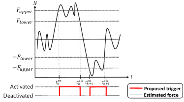
Figure 6: Triggering mechanism developed based on the estimated external force $\hat{F}_{F_{x}}$. As the figure depicts, there are two different thresholds for the activated and deactivated states. The use of thresholds $F_{upper}$ and $F_{lower}$ allows the sensitivity of the trigger to be adjusted.

V-B3 Follower Controller for Longitudinal Motion

To achieve the control objective $F_{Fx}^{B}\rightarrow 0$, a force controller is designed based on the triggering condition developed in Section V-B2 as follows:

$$F_{F_{x}}^{B}=\begin{cases}k_{F_{1}}\hat{v}_{F_{x}}^{B}+\hat{F}_{F_{x}}^{B},&if\;t\in T^{en}\\ k_{F_{2}}\Bigl{(}p_{d,x}-p_{F,x}\Bigr{)},&if\;t\in T^{dis}\end{cases}$$ (71)

where $\hat{v}_{F_{x}}^{B}\in\mathbb{R}$ is the element of the follower velocity:

$$\hat{v}_{F}^{B}\triangleq[\hat{v}_{F_{x}}^{B},\,\hat{v}_{F_{y}}^{B},\,0]^{T}$$

and $\hat{F}_{F_{x}}^{B}$ defined in (27) is estimated by the UKF developed in the Section IV-B, $k_{F_{1}},\,k_{F_{2}}\in\mathbb{R}_{>0}$ are the control gains, $p_{F,x}$ is the first component of follower position $p_{F,x},$ and $p_{d,x}$ is the position along the $X$ axis at the time instant when the triggering condition is switching to $t\in T^{dis}.$ Since $F_{F_{x}}^{B}$ is close to zero, the estimate error can cause vibration, which triggers the second condition to activate the second controller. Since the controller defined in (71) ensures $F_{Fx}^{B}\rightarrow 0,$ the equation of motion for the $x$-axis is neglected.

Remark 7.

$\hat{F}_{F}$ in (71) is estimated from the follower UKF, while $\hat{F}_{F}$ in Fig. 5 is estimated from the leader UKF.

V-B4 Follower Controller for Transverse Motion

The design of this part is based on an impedance controller as depicted in Fig. 7, where the relation between the payload and the follower in the transverse direction can be first modeled as

$$m_{F}\ddot{y}=F_{F_{y}}^{B}-F_{n}^{B},$$ (72)

where $F_{n}^{B}=\frac{m_{p}}{2}a_{n}$ represents the required centripetal force for the payload to follow a curved trajectory, where $a_{n}=\hat{v}_{c_{2,x}}^{2}/\rho\in\mathbb{R}$ represents the centripetal acceleration, with $\rho\in\mathbb{R}$ being the radius of curvature that is obtained based on the latest trajectory approximated by a polynomial based on QP optimization.

Figure 7: The free-body diagram and kinematics of the payload in the transverse direction, and conversion into an impedance control system.

The dynamics in (72) can then be converted into an impedance control system in order to minimize the oscillation between the two so as to achieve nonholonomic motion that satisfies Assumption 3. Force controller $F_{F_{y}}^{B}$ is designed as

$$F_{F_{y}}^{B}=F_{n}^{B}-\frac{m_{F}}{M_{d}}(b_{d}\dot{e}+k_{d}e),$$ (73)

where $e\triangleq y-y_{d}\in\mathbb{R}$ represents the tracking error, $\dot{y}_{d}$ and $\ddot{y}_{d}$ are zero, $M_{d},\,b_{d},\,k_{d}\in\mathbb{R}$ denote the desired inertia, damping, and stiffness, respectively, with $k_{d}$ selected to be $k_{d}=\frac{m_{p}g}{2l_{2}\cos\theta_{y,d}}$ so that the virtual spring force can provide centripetal force $k_{d}y_{d}=F_{n}^{B},$ where $\hat{v}_{F_{x}}$ is used as an alternative of $v$ since $v_{F_{x}}$ is controlled to approach $v$ based on the controller defined in (71), $y=l_{2}\sin\theta_{y},$ where $\mathbf{\theta}_{y}$ satisfies $\cos\theta_{y}=\frac{\nicefrac{{m_{p}g}}{{2}}}{\hat{F}_{F}}$, $y_{d}=l_{2}\sin\theta_{y,d}$ (where $\theta_{y,d}$ satisfies $\tan\theta_{y,d}=\frac{a_{n}}{g}$). The controller described by (73) is designed to achieve $v_{c_{2},y}\rightarrow 0$, but the convergence of $v_{c_{2},y}$ to zero is subject to the accuracy of estimate $\hat{F}_{F_{y}}.$

Substituting (73) into (72) yields the closed-loop dynamics:

$$M_{d}\ddot{e}+b_{d}\dot{e}+k_{d}e=0,$$

where the tracking error goes to zero (i.e., $y\rightarrow y_{d}$) provided that the gains for the second-order linear system are selected properly.

Remark 8.

The follower controller does not require the reference trajectory for controller implementation. In addition, follower controller $F_{F}$ can be estimated from the leader’s UKF and compensated by leader controller $F_{L_{y}}^{B}$ defined in (66).

V-C Low-Level Controller for the Leader and Follower

Similar to (53), the dynamics and the net thrust of the rotors on the UAVs can be given as

$$m_{\zeta}\dot{v}_{\zeta}=T_{\zeta}R_{\zeta}e_{3}-F_{\zeta}-m_{\zeta}ge_{3},$$ (74)

where $e_{3}=\left[\begin{array}[]{ccc}0,&0,&1\end{array}\right]^{T},$ $\zeta\in\left\{L,\,F\right\}$ indicates the leader or follower, $R_{\zeta}\in SO(3)$ denotes the attitude of the UAVs, $F_{\zeta}$ is defined in (26) or (27), and $T_{\zeta}\in\mathbb{R}$ represents the net thrust generated by the rotors on the UAV. Based on [39], the geometric tracking controller for the leader and follower UAVs is designed as

$$T_{\zeta} =\left(F_{\zeta}+m_{\zeta}ge_{3}+m_{\zeta}\dot{v}_{\zeta,d}\right)\cdot R_{\zeta}e_{3},$$ (75)

$$M_{\zeta} =k_{e,\zeta}e_{R_{\zeta}}+k_{\Omega,\zeta}e_{\Omega_{\zeta}}+\Omega_{\zeta}\times J_{\zeta}\Omega_{\zeta}$$

$$-J_{\zeta}(\left[\Omega_{\zeta}\right]_{\times}R_{\zeta}^{T}R_{\zeta,d}\Omega_{\zeta,d}-R_{\zeta}^{T}R_{\zeta,d}\dot{\Omega}_{\zeta,d}),$$ (76)

where $F_{\zeta}$ are force controllers defined in (65), (66), (71), and (73), $\dot{v}_{\zeta,d}\in\mathbb{R}^{3}$ represents the reference acceleration, $k_{e,\zeta},\,k_{\Omega,\zeta}\in\mathbb{R}$ are positive control gains, $\Omega_{\zeta}\in\mathbb{R}^{3}$ is defined as the angular velocity of the UAV, $R_{\zeta,d},\,\Omega_{\zeta,d}\in\mathbb{R}^{3}$ represent the reference attitude and reference angular velocity of the UAV, respectively, and attitude error $e_{R_{\zeta}}$ and angular velocity error $e_{\Omega_{\zeta}}$ of the UAV are defined as

$$e_{R_{\zeta}} =\frac{1}{2}\left(R_{\zeta,d}^{T}R_{\zeta}-R_{\zeta}^{T}R_{\zeta,d}\right)$$ (77)

$$e_{\Omega_{\zeta}} =\Omega_{\zeta}-R_{\zeta}^{T}R_{\zeta,d}\Omega_{\zeta,d}.$$ (78)

The thrust command for each rotor on the UAV can be obtained based on the following relation:

$$\left[\begin{array}[]{c}T_{\zeta}\\ M_{\zeta,x}\\ M_{\zeta,y}\\ M_{\zeta,z}\end{array}\right]=\varGamma\left[\begin{array}[]{c}f_{\zeta}^{1}\\ f_{\zeta}^{2}\\ \vdots\\ f_{\zeta}^{n}\end{array}\right],$$ (79)

where $\varGamma\in\mathbb{R}^{4\times n}$ is a control allocation matrix. In (79), $f_{\zeta}^{i}$ represents the thrust corresponding to the $i^{\text{th}}$ rotors of the UAV, which is assumed to be proportional to the square of angular velocity $\omega_{\zeta}^{i},$ and is expressed as

$$f_{\zeta}^{i}=k_{\zeta}^{i}\left(\omega_{\zeta}^{i}\right)^{2},\ i=1,\,2,\,\ldots,\,n.$$ (80)

where $n\in\mathbb{R}$ is the number of rotors, and $k_{\zeta}^{i}$ is a positive constant.

V-D System Architecture

To make the system architecture clear, the dynamics and controllers of each subsystem are summarized in Table IV.

Table IV: Dynamics and controllers.

Subsystem	Type	Equation(s)
Payload	Kinematics	(23)
	Dynamics	(48) and (49)
Leader	Kinematics controller	(67)
	Dynamics controller ($x$ and $y$ axes)	(65) and (66)
Follower	Kinematics controller	(72)
	Dynamics controller ($x$ and $y$ axes)	(71) and (73)
Flight controller	Low-level controller	(75) and (76)

VI Stability Analysis

VI-A Stability Analysis of the Leader Controller

As mentioned in Section V-B, the follower is controlled to avoid transverse motion and the tracking error will be compensated by the leader controller. Therefore, only the tracking performance of the leader controller is provided in this section. To this end, a Lyapunov-based approach is developed to analyze the stability of the closed-loop system.

Theorem 1.

Given a leader-follower system as depicted in Fig. 2, the leader controller defined in (65) and (66) ensures that the system can achieve asymptotic tracking as defined in (8).

Proof:

Let a Lyapunov function be defined as

$$V_{1}=\frac{1}{2}x_{e}^{2}+\frac{1}{2}y_{e}^{2}+\frac{1-\cos\left(\theta_{e}\right)}{k_{2}},$$ (81)

where $x_{e}$, $y_{e}$ and $\theta_{e}$ are the tracking errors defined in (6) and (7), and $k_{2}$ is a positive constant. Substituting the controller defined in (67) into (23) yields the closed-loop error dynamics:

$$\begin{cases}\dot{x}_{e}=\omega y_{e}-k_{1}x_{e}+\eta_{1}\\ \dot{y}_{e}=-\omega(x_{e})+v_{r}\sin\theta_{e}\\ \dot{\theta}_{e}=-v_{r}k_{2}y_{e}-k_{3}\sin\theta_{e}+\eta_{2}\end{cases},$$ (82)

where $k_{1}$ and $k_{3}$ are positive constants. Taking the time derivative of the Lyapunov function defined in (81) and using (82) yields

$$\dot{V}_{1}= x_{e}\left(\omega y_{e}-k_{1}x_{e}+\eta_{1}\right)$$

$$+y_{e}(-\omega x_{e})+y_{e}v_{r}\sin\theta_{e}$$

$$+(-v_{r}k_{2}y_{e}-k_{3}\sin\theta_{e}+\eta_{2})\frac{\sin\theta_{e}}{k_{2}},$$ (83)

and canceling out the cross terms reduces (83) to

$$\dot{V}_{1}=-k_{1}x_{e}^{2}-\frac{k_{3}\left(\sin\theta_{e}\right)^{2}}{k_{2}}+x_{e}\eta_{1}+\frac{\sin\theta_{e}}{k_{2}}\eta_{2}.$$ (84)

A second Lyapunov function that contains $V_{1}$ is now defined as

$$V_{2}=V_{1}+\frac{1}{2}\eta_{1}^{2}+\frac{1}{2}\eta_{2}^{2},$$ (85)

where $\eta_{1},\eta_{2}$ are defined in (24) and (25). Taking the time derivative of the Lyapunov function in (85) yields

$$\dot{V}_{2}=\dot{V}_{1}+\eta_{1}\dot{\eta}_{1}+\eta_{2}\dot{\eta}_{2}.$$ (86)

Taking the time derivative of (24) and (25) and substituting the controllers defined in (65) and (66) into the open-loop dynamics (48) and (49) along with the result in (68) yields the closed-loop error system as:

$$\dot{\eta}_{1} =-k_{v}\eta_{1}-x_{e}$$ (87)

$$\dot{\eta}_{2} =-k_{\omega}\eta_{2}-\frac{\sin\theta_{e}}{k_{2}}.$$ (88)

Substituting (87) and (88) into (86) and using (84) yields

$$\dot{V}_{2}=-k_{v}\eta_{1}^{2}-k_{\omega}\eta_{2}^{2}-k_{1}x_{e}^{2}-\frac{k_{3}\left(\sin\theta_{e}\right)^{2}}{k_{2}},$$ (89)

which is a negative semidefinite function provided that $k_{v},$ $k_{\omega},$ $k_{1}$, $k_{2},$ and $k_{3}$ are selected to be positive constants. Therefore, LaSalle’s invariance principle can be invoked to show

$$\begin{array}[]{cc}\begin{array}[]{c}x_{e}\rightarrow 0\\ y_{e}\rightarrow 0\\ \theta_{e}\rightarrow 0\\ \eta_{1}\rightarrow 0\\ \eta_{2}\rightarrow 0\end{array}&\text{as }t\rightarrow\infty,\end{array}$$ (90)

which implies that the control objective defined in (8) is achieved. ∎

VI-B Robustness of the Leader Controller

To consider the robustness of the leader controller, the estimate errors from the UKFs are added into the leader controller defined in (65) and (66) as

$$F_{L_{x}}= m_{p}\left(\dot{v}_{d}+x_{e}+k_{v}\eta_{1}+r_{\nicefrac{{c_{2}}}{{p,x}}}\omega^{2}\right)+d_{1}$$ (91)

$$F_{L_{y}}= -\frac{2I_{zz}}{L}\left(\dot{\omega}_{d}+k_{\omega}\eta_{2}+\frac{\sin\theta_{e}}{k_{2}}\right)+F_{F_{y}}+d_{2},$$ (92)

where $d_{1},\,d_{2}\in\mathbb{R}$ are the additive terms that include the estimator errors (e.g., $\hat{p}_{c_{2}}-p_{c_{2}},$ $\hat{v}-v,$ $\hat{F}_{F_{y}}-F_{F_{y}}$) from the UKFs and the disturbances. By substituting (91) and (92) into the same Lyapunov function, $\dot{V}_{2}$ can be upper bounded as

$$\dot{V}_{2} \leq-k_{v}\eta_{1}^{2}-k_{\omega}\eta_{2}^{2}-k_{1}x_{e}^{2}-\frac{k_{3}\left(\sin\theta_{e}\right)^{2}}{k_{2}}+D_{1}\left|\eta_{1}\right|+D_{2}\left|\eta_{2}\right|,$$ (93)

where $D_{1},\,D_{2}\in\mathbb{R}_{>0}$ are positive constant upper bounds of the estimate errors and disturbances. After completing the square, (93) can be further upper bounded as

$$\dot{V}_{2} \leq-k_{v1}\eta_{1}^{2}-k_{\omega 1}\eta_{2}^{2}-k_{1}x_{e}^{2}-\frac{k_{3}\left(\sin\theta_{e}\right)^{2}}{k_{2}}+\frac{D_{1}^{2}}{4k_{v2}}+\frac{D_{2}^{2}}{4k_{\omega 2}},$$ (94)

where $k_{v1},\,k_{v2},\,k_{\omega 1},\,k_{\omega 2}\in\mathbb{R}_{>0}$ satisfy $k_{v}=k_{v1}+k_{v2}$ and $k_{\omega}=k_{\omega 1}+k_{\omega 2}$. (93) implies that tracking error $p_{e}$ and $\theta_{e}$ defined in (6) and (7) are uniformly ultimately bounded, and the error bounds can be decreased by increasing the control gains $k_{v},\,k_{\omega},$ and $k_{1}.$

VII Motion Planning for the Leader-Follower System

In general cases, obstacles and physical constraints are taken into account when planning an optimal trajectory. This section divides the motion planning for the leader-follower system into two parts: trajectory planning and trajectory generation.

VII-A Trajectory Planning

[40] proposed using a hybrid A* planner to find the correct trajectory for a nonholonomic vehicle in an environment with obstacles from the start to the end point under various constraints such as nonholonomic motion and the dimensions of the vehicles. The information about the environment is digitized to a bitmap before performing the planning; for example, the location of obstacles in the environment are considered as 1 and are shown in black in Fig. 8. The planner output is a sequence of waypoints.

Figure 8: The leader-follower system executing a cooperative transportation task.

VII-B Trajectory Generation

To generate a desired trajectory for the UAV, [31] used QP to find the minimun-snap trajectory passing through all of the waypoints. Let each trajectory segment presented by a polynomial be defined as

$$s_{i}(t)=\sum_{j=0}^{N}a_{ij}t^{j},\ t_{i-1}\leq t\leq t_{i},\ i\in\{1,\ 2,\ldots,\ M\},$$ (95)

where $a_{ij}\in\mathbb{R}$ is the $j^{\text{th}}$ order coefficient, $N\in\mathbb{N}$ represents the order of the polynomial, $M\in\mathbb{N}$ represents the total number of segments, and $t_{i}$ is the time when $c_{2}$ passes through the $i^{\text{th}}$ waypoint. To generate a smooth trajectory, $N=7$ is selected to minimize the snap of $s_{i}$ so that Assumption 4 can be satisfied and cost function $J$ is expressed as

$$J =\underset{a_{ij}}{\min}\sum_{i=1}^{n}\int_{t_{i-1}}^{t_{i}}\|\frac{d^{4}s_{i}(t)}{dt^{4}}\|^{2}dt$$ (96)

$$\text{s.t.}\ AT=B,$$

where $A$ is a matrix consisting of coefficient $a_{ij}$, $T$ is a vector consisting of the time intervals defined in (95), and $B$ is a vector determined by the waypoints. The optimal solution of (96) is found using a QP solver [31].

VIII Simulations

Two simulations of the leader-follower system were performed. Simulation 1 evaluated the tracking performance of the developed controller, including the leader and follower controllers. Moreover, the estimation performance of the UKFs were also determined to ensure they provide accurate estimates for control feedback. After evaluating the control performance in Simulation 1, Simulation 2 was performed to show that the leader can change the desired trajectory in real time during flight.

VIII-A Implementation

The simulations were conducted using the ROS and Gazebo simulator with the UAV model from RotorS provided by [41] along with a customized payload model. All of the ground truth was provided by the simulator.

VIII-B Simulation 1: Evaluation of the Tracking Controller

Simulation 1 was divided into two parts: (1) evaluating the controller for tracking a desired trajectory, and (2) evaluating the performance of the UKFs for the UAVs.

VIII-B1 Evaluation of the Controller

Fig. 9 shows that the system can track a desired trajectory, which is a high-order polynomial solved by the QP solver in the leader UAV.

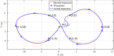
Figure 9: Desired trajectory generated from the QP solver and the actual trajectory of point $c_{2}.$

The positions of the waypoints are listed as in Table V.

Table V: All segments in the trajectory.

Segment	Start-End	Duration (s)
1	$(1,1)-(3,5)$	$16.0$
2	$(3,5)-(12,0)$	$16.0$
3	$(12,0)-(3,-5)$	$16.0$
4	$(3,-5)-(-3,5)$	$16.0$
5	$(-3,5)-(-12,0)$	$16.0$
$6$	$(-12,0)-(-3,-5)$	$16.0$
7	$(-3,-5)-(0,0)$	$16.0$

Figs. 10 and 11 show the tracking errors during the cooperative transportation. $x_{c_{2}}$ and $y_{c_{2}}$ represent the position of $c_{2}$ along the $X$ and $Y$ axes of the inertial frame. Both tracking errors $x_{e}$ and $y_{e}$ decreased over time. Also, the tracking error in the transverse direction increased as the curvature increased, and decreased rapidly while traveling along a straight trajectory, which can be attributed to the efficacy of the impedance controller since the desired trajectory and the curvature are not available to the follower. The standard deviations of $x_{e}$ and $y_{e}$ were $0.36$ m and $0.41$m, respectively.

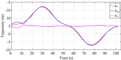
Figure 10: Position and tracking error of point $c_{2}$ along the $X$ axis of the inertial frame.

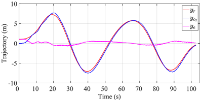
Figure 11: Position and tracking error of point $c_{2}$ along the $Y$ axis of the inertial frame.

Figs. 12 and 13 show the tracking performance of the kinematics controller defined in (67). Signals $\eta_{1}$ and $\eta_{2}$ are close to zero in the steady state, and the oscillation is due to the payload swinging along $x^{B}$ during flight and corresponds to position errors that are compensated by the leader controller.

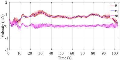
Figure 12: $\hat{v}$ is estimated by the UKF in Section IV-C2, and $v_{d}$ is the desired linear velocity in (67). Signal $\eta_{1}$ indicates the tracking performance of the leader controller during translational motion.

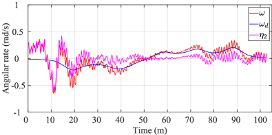
Figure 13: $\omega$ is measured by the IMU attached to the payload at $c_{1},$ and $\omega_{d}$ is the desired angular rate in (67). Signal $\eta_{2}$ indicates the tracking performance of the leader controller during rotational motion.

Figs. 14 and 15 show the actual and desired forces applied to point $c_{1}$ by the leader, which implies that the geometric controller can achieve force control as described by (74).

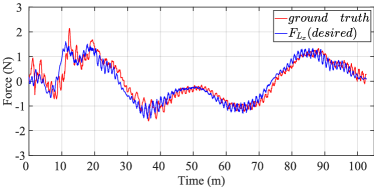
Figure 14: The ground truth of $F_{L_{x}}$estimated by the virtual force sensor on the payload, and desired force $F_{L_{x}}$ computed by the leader controller, both expressed in the inertial frame.

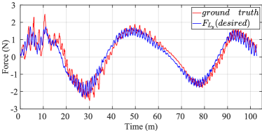
Figure 15: The ground truth of $\hat{F}_{L_{y}}$ estimated by the virtual force sensor on the payload, and desired force $F_{L_{y}}$ computed by the leader controller, both expressed in the inertial frame.

Table VI: RMSE values of the error signals in the leader controller.

RMSE	Value	Unit
$x_{e}$	$0.36$	m
$y_{e}$	$0.42$	m
$\eta_{1}$	$0.13$	$\text{m}/\text{s}$
$\eta_{2}$	$0.13$	$\text{rad}/\text{s}$

To assess the performance of the UKF in Section IV-C2, Figs. 16 and 17 show the difference between the estimation and the ground truth. Velocity $\hat{v}$ estimated by the leader UKF is very close to the ground truth.

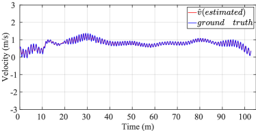
Figure 16: $\hat{v}$ estimated by the second UKF in (64) is close to the ground truth, which implies that the UKFs perform well.

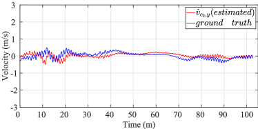
Figure 17: Estimated transverse velocity $\hat{v}_{c_{2},y}$ is essentially not zero, which satisfies Assumption 3. Nevertheless, the tracking error in the transverse direction can be compensated by the leader controller as indicated in Fig. 9.

VIII-B2 Evaluation of the UKFs

Figs. 18 and 19 show estimated forces $\hat{F}_{F_{x}}$ and $\hat{F}_{F_{y}}.$

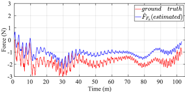
Figure 18: Estimate $\hat{F}_{F_{x}}$ is not sufficiently accurate since the rotors defined in (80) is not well modeled. However, the mismatch can be compensated for by analyzing the effects of $d_{1}$ on system stability using (91).

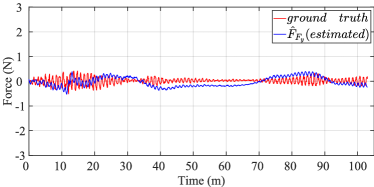
Figure 19: Estimate $\hat{F}_{F_{y}}$ is not sufficiently accurate since the rotors defined in (80) is not well modeled; however, the mismatch can be compensated for by analyzing the effects of $d_{2}$ on system stability using (92).

Fig. 20 shows the effect of the triggering event described in Section V-B2.

Figure 20: A triggering signal of $1$ implies $t\in T^{en},$ while it is $0$ otherwise. The trigger switches frequently at the beginning, while no switching occurs thereafter since the estimated force is far from zero in the steady state.

Table VII: RMSE values of the estimates of the first UKF for the follower.

RMSE	Value	Unit
$\hat{F}_{F_{x}}$	0.75	N
$\hat{F}_{F_{y}}$	0.25	N

Table VIII: Simulation results with different disturbances and noise. The disturbances of UAV $i\in\left\{L,\,F\right\}$ were obtained from a zero-mean normal distribution with variance $\sigma_{i}$ defined as $\mathcal{N}_{i}(0,\sigma_{i}),$ and the noise was also obtained from a zero-mean normal distribution.

Simulation	Disturbances		Noise		Errors
	Leader	Follower	Accelerometer	Gyro	$x_{e}$	$y_{e}$	$\eta_{1}$	$\eta_{2}$	$\hat{F}_{F_{x}}$	$\hat{F}_{F_{y}}$
1	$\mathcal{N}_{L}(0,0.5)$	$\mathcal{N}_{F}(0,0.5)$	$\mathcal{N}(0,1)$	$\mathcal{N}(0,0081)$	0.75	0.69	0.33	0.29	0.88	0.4
2	$\mathcal{N}_{L}(0,1.5)$	$\mathcal{N}_{F}(0,0.5)$			0.77	0.82	0.52	0.6	1.56	1.28
3	$\mathcal{N}_{L}(0,1.5)$	$\mathcal{N}_{F}(0,1.5)$			0.9	0.82	0.55	0.56	1.3	0.7

VIII-C Simulation 2: Changing the Trajectory of the Payload During Flight

The tracking performance of the controllers are evaluated in Section VIII-B. Another simulation was conducted to evaluate the efficacy of the control architecture that allows changing the desired trajectory in real time. The system starts from the blue dot in Fig. 21, and attempted to follow a double circular trajectory like that shown in Fig. 9 until $c_{2}$ point on the payload reached the green star. At that instant, the leader decided to transit $c_{2}$ from desired trajectory 1 to desired trajectory 2, and the follower was not aware of the transition. Fig. 21 indicates that the controller can ensure good tracking performance while traveling along a straight trajectory, and that the tracking error increases as the curvature increases, which can again be attributed to the efficacy of the impedance controller since the desired trajectory and the curvature are not available to the follower.

Figure 21: Trajectories 1 and 2. The leader-follower transportation system started at the blue dot from trajectory 1 and transited to trajectory 2 at the green star in real time.

VIII-D System Parameters

The system parameters and control gains used in the simulations are listed in Table IX and X, respectively .

Table IX: The system parameters.

Parameter	$m_{p}$	$I_{zz}$	$L$	$l_{1}$	$l_{2}$	$F_{upper}$	$F_{lower}$
Value	$0.5$	$0.083$	$1$	$0.18$	$0.18$	$0.3$	$0.2$
Unit	kg	$\text{kg}\text{m}^{2}$	m	m	m	N	N

Table X: Control gains.

Gain	$k_{1}$	$k_{2}$	$k_{3}$	$k_{v}$	$k_{\omega}$
Value	3	1	5	5	11

  Gain $k_{F_{1}}$ $k_{F_{2}}$ $k_{d}$ $b_{d}$ $M_{d}$ Value 1 3 13.6 2.0 1.5

VIII-E Simulations with Noise and Disturbances

To make the simulations more-accurate representations of experiments, noise was added to the IMU and disturbances of various magnitudes were added to the UAVs to verify the system stability. The simulation results are summarized in Table VIII.

The noise was the same for all three simulations. The errors increased from simulation 1 to simulation 2, since the disturbances in the leader UAV increased, and similarly from simulation 2 to simulation 3 as the disturbances in the follower increased. The simulations indicate that the UAV could successfully complete all of the cooperative transportation tasks. These simulation findings verify the control effectiveness of the developed controller.

IX Experiments

Experiments were performed to evaluate the tracking performance of the leader and follower controllers. Moreover, the estimation performance of the UKFs was also determined to ensure they provide accurate estimates for control feedback.

IX-A Implementation

IX-A1 Hardware

A DJI F450 UAV was used in the experiments. This multirotor was equipped with XBee modules to allow communication between the multirotor and the ground station for monitoring and collecting data. Angular velocity and acceleration for obtaining the attitude of the multirotor were measured using the IMU, and the position of the multirotor was measured using a motion capture system (Optitrack). Companion computers (i.e., x5-Z8350 from AAEON) were implemented on the UAVs for computing the UKFs. The two ends of the payload were connected to the UAVs with ropes. The configuration of the multirotor is shown in Fig. 22.

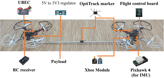
Figure 22: Hardware architecture.

IX-A2 Software

The developed controller and the UKFs were implemented on an ROS (Robot Operating System) in the companion computers. Since the controller and UKFs are implemented on the follower and leader, no inter-agent communication is required. The leader controller was computed on the UP board, and the follower controller was computed on the flight control board.

IX-A3 System Parameters

The system parameters and control gains used in the experiments are listed in Tables XI and XII, respectively. The upper and lower bounds of the leader controller are listed in Table XIII.

Table XI: System parameters.

Parameter	$m_{p}$	$I_{zz}$	$L$	$l_{1}$	$l_{2}$	$F_{upper}$	$F_{lower}$
Value	$0.5$	$0.1053$	$1.59$	$0.2$	$0.2$	$0.3$	$0.25$
Unit	kg	$\text{kg}\text{m}^{2}$	m	m	m	N	N

Table XII: Control gains.

Gain	$k_{1}$	$k_{2}$	$k_{3}$	$k_{v}$	$k_{\omega}$
Value	3	0.1	1	3	30

  Gain $k_{F_{1}}$ $k_{F_{2}}$ $k_{d}$ $b_{d}$ $M_{d}$ Value 0.04 4 12.26 2.0 2

Table XIII: Upper and lower bounds of the leader controller.

Direction	$\mathit{x}$	$\mathit{y}$
Upper bound (N)	2.0	10.0
Lower bound (N)	-2.6	-7.0

IX-B Evaluation of the Tracking Controller

The experiments were divided into two parts: (1) evaluating the controller by tracking a desired trajectory and (2) evaluating the performance of the UKFs for the UAVs.

IX-B1 Evaluation of the Controller

Figs. 23 and 24 show that the system can track a desired trajectory, which is a high-order polynomial solved by the companion computer on the leader UAV.

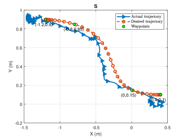
Figure 23: Desired trajectory S and the actual trajectory of point $c_{2}$.

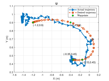
Figure 24: Desired trajectory U and the actual trajectory of point $c_{2}$.

The waypoints of trajectories S and U are listed in Tables XIV and XV, respectively. The position RMSE of the trajectory tracking is listed in Table XVI. The tracking errors were greatly affected by airflow disturbance due to the experiments being conducted in a restricted space.

Table XIV: All segments in trajectory S.

Segment	Start - End	Duration (s)
1	$(-1.20,0.90)-(-0.80,0.85)$	$5.0$
2	$(-0.80,0.85)-(0.00,0.15)$	$6.0$
3	$(0.00,0.15)-(0.40,0.10)$	$5.0$

Table XV: All segments in trajectory U.

Segment	Start - End	Duration (s)
1	$(-1.20,0.90)-(-0.40,0.90)$	$7.0$
2	$(-0.40,0.90)-(-0.15,0.45)$	$5.0$
3	$(-0.15,0.45)-(-0.35,0.45)$	$3.0$

Table XVI: RMSEs of the two trajectories.

Trajectory	S		U
	$\mathit{x}$ (m)	$\mathit{y}$ (m)	$\mathit{x}$ (m)	$\mathit{y}$ (m)
RMSE	0.3176	0.1366	0.2835	0.1376
Geometric RMSE	0.3457		0.3151

Figs. 25 and 26 show the trajectories and the tracking errors during the cooperative transportation. $x_{c_{2}}$ and $y_{c_{2}}$ represent the position of $c_{2}$ along the $X$ and $Y$ axes in the inertial frame. The tracking error in the transverse direction increased as the curvature increased, and decreased rapidly while traveling along a straight trajectory. This behavior can be attributed to the efficacy of the impedance controller, since the desired trajectory and the curvature are not available to the follower. Table XVII lists the standard deviations of $x_{e}$ and $y_{e}$ for the two trajectories.

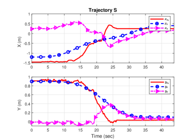
Figure 25: Position and tracking errors of point $c_{2}$ along the $X$ and $Y$ axes in the inertial frame for trajectory S.

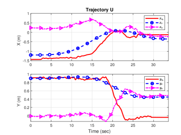
Figure 26: Position and tracking errors of point $c_{2}$ along the $X$ and $Y$ axes in the inertial frame for trajectory U.

Table XVII: Standard deviations of the two trajectories.

Trajectory	S		U
	$\mathit{x}$	$\mathit{y}$	$\mathit{x}$	$\mathit{y}$
Standard deviations (m)	0.3063	0.1176	0.2465	0.2479

Figs. 27, 28, 29, and 30 show the tracking performance of the kinematics controller designed in (67) when tracking trajectories S and U. The oscillation of signals $\eta_{1}$ and $\eta_{2}$ is due to the payload swinging along the $x^{B}$ direction during the flight, and corresponds to the position errors that are compensated by the leader controller.

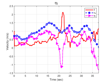
Figure 27: Trajectory S. $\hat{v}$ is estimated by the UKF described in Section IV-C2, and $v_{d}$ is the desired velocity according to (67). Signal $\eta_{1}$ indicates the tracking error of the leader controller during translational motion.

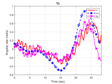
Figure 28: Trajectory S. $\omega$ is measured by the IMU attached to the payload at $c_{1},$ and $\omega_{d}$ is the desired angular rate according to (67). Signal $\eta_{2}$ indicates the tracking error of the leader controller during rotational motion.

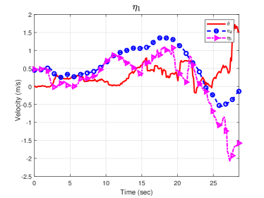
Figure 29: Trajectory U. $\hat{v}$ is estimated by the UKF described in Section IV-C2, and $v_{d}$ is the desired velocity according to (67). Signal $\eta_{1}$ indicates the tracking error of the leader controller during translational motion.

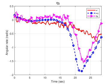
Figure 30: Trajectory U. $\omega$ is measured by the IMU attached to the payload at $c_{1},$ and $\omega_{d}$ is the desired angular rate according to (67). Signal $\eta_{2}$ indicates the tracking error of the leader controller during rotational motion.

Figs. 31 and 32 show the desired forces applied to point $c_{1}$ by the leader. The upper and lower bounds are set to prevent aggressive control inputs, since the rope is not a rigid body. A delay is present because the leader controller was designed to track the desired $\mathit{c_{2}},$ point which is not located on the leader itself.

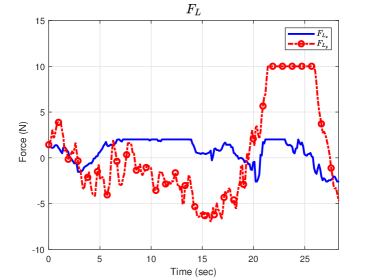
Figure 31: Desired forces $F_{L_{x}}$ and $\mathit{F_{L_{y}}}$ for trajectory S computed by the leader controller, both expressed in the body frame.

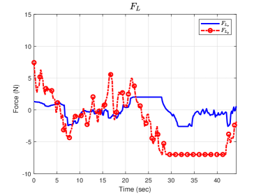
Figure 32: Desired forces $F_{L_{x}}$ and $\mathit{F_{L_{y}}}$ for trajectory U computed by the leader controller, both expressed in the body frame.

IX-B2 Evaluation of the UKFs

Figs. 33 and 34 show follower force estimates $\hat{F}_{F_{x}}$ and $\hat{F}_{F_{y}}$ when tracking trajectories S and U. Estimate $\mathit{\hat{F}_{F_{y}}}$ is close to zero due to the nonholonomic constraint, and $\mathit{\hat{F}_{F_{x}}}$ almost remains positive since the leader pulls the follower during the motion.

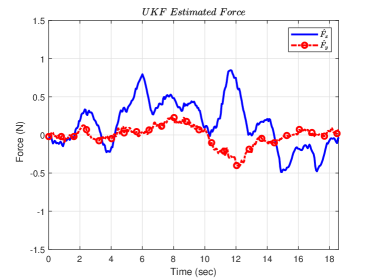
Figure 33: Forces estimated by the follower UKF for trajectory S.

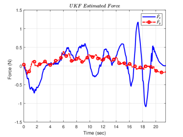
Figure 34: Forces estimated by the follower UKF for trajectory U.

Figs. 35 and 36 show the effects of triggering events, as designed in Section V-B2, when tracking trajectories S and U. Zeno behavior did not occur due to the presence of only a few triggers.

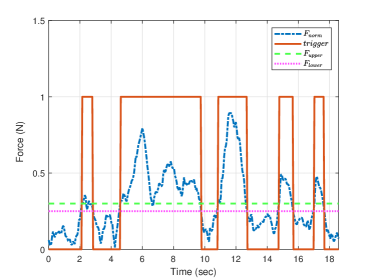
Figure 35: Trajectory S. A triggering signal of $1$ implies $t\in T^{en},$ while it is $0$ otherwise.

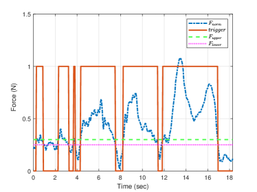
Figure 36: Trajectory U. A triggering signal of $1$ implies $t\in T^{en},$ while it is $0$ otherwise.

X Discussion

A cooperative transportation using a leader-follower UAV system has been developed, in which inter-UAV communication is not required and the reference trajectory of the payload can be modified in real time. To achieve this, the system is modeled as a nonholonomic system such that the follower’s motion does not affect the tracking error of the payload; that is, the follower is controlled such that one end of the payload performs only longitudinal motion, and the leader is controlled to ensure asymptotic tracking of the $c_{2}$ point on the payload. Robustness of the leader controller is also proven given the estimate errors in the UKFs and the disturbances. UKFs are developed to estimate the forces applied by the leader and follower so that force sensors are not required. Stability analysis has proven the stability of the closed-loop system. Simulations have demonstrated the performance of the tracking controller and the feasibility of changing the desired trajectories online. The experiments show the controllers of the leader and the follower can work in the real world, but the tracking errors were greatly affected by the disturbance of airflow in a restricted space. Future works will consider new control approaches based on more-practical IMU setups and the instability caused by the disturbances.

References

- [1] H. Yamaguchi, M. Mori, and A. Kawakami, “A path following feedback control method using parametric curves for a cooperative transportation system with two car-like mobile robots,” IFAC Proc. Vol., vol. 43, no. 16, pp. 163–168, 2010.
- [2] A. Yufka, O. Parlaktuna, and M. Ozkan, “Formation-based cooperative transportation by a group of non-holonomic mobile robots,” in IEEE Int. Conf. Syst. Man Cybern., Istanbul, Turkey, Oct. 2010, pp. 3300–3307.
- [3] A. Petitti, A. Franchi, D. D. Paola, and A. Rizzo, “Decentralized motion control for cooperative manipulation with a team of networked mobile manipulators,” in IEEE Int. Conf. Robot. Autom., May 2016, pp. 441–446.
- [4] A. Marino and F. Pierri, “A two stage approach for distributed cooperative manipulation of unknown object without explicit communication and unknown number of robots,” in Robot. Auton. Syst., vol. 103, 2018, pp. 122–133.
- [5] Z. Wang and M. Schwager, “Kinematic multi-robot manipulation with no communication using force feedback,” in Proc. IEEE Int. Conf. Robot. Autom., May 2016, pp. 427–432.
- [6] Z. Wang and M. Schwager, “Force-amplifying n-robot transport system (force-ants) for cooperative planar manipulation without communication,” in Int. J. Robot. Res., vol. 35, no. 13, 2016, pp. 1564–1586.
- [7] Z. Wang and M. Schwager, “Multi-robot manipulation with no communication using only local measurements,” in IEEE Conf. Decis.Control, 2015, pp. 380–385.
- [8] C. K. Verginis, A. Nikou, and D. V. Dimarogonas, “Communication-based decentralized cooperative object transportation using nonlinear model predictive control,” in European Control Conf., Limassol, Cyprus, Jun. 2018.
- [9] A. Tsiamis, C. K. Verginis, C. P. Bechlioulis, and K. J. Kyriakopoulos, “Cooperative manipulation exploiting only implicit communication,” in IEEE/RSJ Int. Conf. Intell. Robots Syst., Hamburg, Germany, Sep. 2015, pp. 864–869.
- [10] A. Tsiamis, C. P. Bechlioulis, G. C. Karras, and K. J. Kyriakopoulos, “Decentralized object transportation by two nonholonomic mobile robots exploiting only implicit communication,” in IEEE Int. Conf. Robot. Autom., 2015, pp. 171–176.
- [11] T. Fan, H. Weng, and T. Murphey, “Decentralized and recursive identification for cooperative manipulation of unknown rigid body with local measurements,” in IEEE Conf. Decis. Control, Melbourne, Australia, Dec. 2017, pp. 2842–2849.
- [12] P. Culbertson and M. Schwager, “Decentralized adaptive control for collaborative manipulation,” in IEEE Int. Conf. Robotics Autom., Brisbane, Australia, May 2018, pp. 278–285.
- [13] C. P. Bechlioulis and K. Kyriakopoulos, “Collaborative multi-robot transportation in obstacle-cluttered environments via implicit communication,” in Front. Robot. AI, vol. 5, 2018, p. 90.
- [14] Y. Yang, H. Modares, K. G. Vamvoudakis, Y. Yin, and D. C. Wunsch, “Dynamic intermittent feedback design for containment control on a directed graph,” IEEE Trans. Cybern., pp. 1–14, 2019.
- [15] K. Sreenath and V. Kumar, “Dynamics, control and planning for cooperative manipulation of payloads suspended by cables from multiple quadrotor robots,” in Proc. Robot., Sci. Syst., Berlin, Germany, Jun. 2013.
- [16] H. Lee, H. Kim, and H. J. Kim, “Path planning and control of multiple aerial manipulators for a cooperative transportation,” in IEEE/RSJ Int. Conf. Intell. Robots Syst., Hamburg, Germany, Sep. 2015, pp. 2386–2391.
- [17] T. Lee, K. Sreenath, and V. Kumar, “Geometric control of cooperating multiple quadrotor UAVs with a suspended payload,” in IEEE Conf. Decis. Control, Florence, Italy, Dec. 2013, pp. 5510–5515.
- [18] A. S. Aghdam, M. B. Menhaj, F. Barazandeh, and F. Abdollahi, “Cooperative load transport with movable load center of mass using multiple quadrotor UAVs,” in Int. Conf. Control Instrum. Autom., Qazvin Islamic Azad University, Qazvin, Iran, Jan. 2016, pp. 23–27.
- [19] Y.-H. Lim, S.-H. Kwon, K.-H. Kim, and H.-S. Ahn, “Implementation of load transportation using multiple quadcopters,” in IEEE Int. Conf. Adv. Intell. Mechatron., Munich, Germany, Jul. 2017, pp. 639–644.
- [20] Y. Liu, Q. Wang, H. Hu, and Y. He, “A novel real-time moving target tracking and path planning system for a quadrotor UAV in unknown unstructured outdoor scenes,” IEEE Trans. Syst., Man, Cybern., Syst., vol. 49, no. 11, pp. 2362–2372, Nov 2019.
- [21] N. Wang, S. Su, M. Han, and W. Chen, “Backpropagating constraints-based trajectory tracking control of a quadrotor with constrained actuator dynamics and complex unknowns,” IEEE Trans. Syst., Man, Cybern., Syst., vol. 49, no. 7, pp. 1322–1337, July 2019.
- [22] M. Chen, S. Xiong, and Q. Wu, “Tracking flight control of quadrotor based on disturbance observer,” IEEE Trans. Syst., Man, Cybern., Syst., pp. 1–10, 2019.
- [23] Y. Yang, K. G. Vamvoudakis, H. Modares, Y. Yin, and D. C. Wunsch, “Hamiltonian-driven hybrid adaptive dynamic programming,” IEEE Trans. Syst., Man, Cybern., Syst., pp. 1–12, 2020.
- [24] H. Lee and H. J. Kim, “Constraint-based cooperative control of multiple aerial manipulators for handling an unknown payload,” IEEE Trans. Industrial Inform., vol. 13, no. 6, pp. 2780–2790, Dec. 2017.
- [25] C. Masone, H. H. Bï¿œlthoff, and P. Stegagno, “Cooperative transportation of a payload using quadrotors: a reconfigurable cable-driven parallel robot,” in IEEE/RSJ Int. Conf. Intell. Robots Syst., Daejeon, Korea, Oct. 2016, pp. 1623–1630.
- [26] G. Loianno and V. Kumar, “Cooperative transportation using small quadrotors using monocular vision and inertial sensing,” IEEE Robot. Autom. Lett., vol. 3, no. 2, pp. 680–687, Apr. 2018.
- [27] T. Lee, “Geometric control of quadrotor UAVs transporting a cable-suspended rigid body,” IEEE Trans. Control Syst. Technol., vol. 26, no. 1, pp. 255–264, Jan. 2018.
- [28] M. Tognon, C. Gabellieri, L. Pallottino, and A. Franchi, “Aerial co-manipulation with cables: The role of internal force for equilibria, stability, and passivity,” in IEEE Robot. Autom. Lett., vol. 3, no. 3, 2018, pp. 2577–2583.
- [29] N. Michael, J. Fink, and V. Kumar, “Cooperative manipulation and transportation with aerial robots,” in Proc. Robot., Sci. Syst., Seattle, WA, USA, Jun. 2009, pp. 73–86.
- [30] D. Sanalitro, H. J. Savino, M. Tognon, J. Cortés, and A. Franchi, “Full-pose manipulation control of a cable-suspended load with multiple UAVs under uncertainties,” IEEE Robot. Autom. Lett., vol. 5, no. 2, pp. 2185–2191, 2020.
- [31] Z. Wang, S. Singh, M. Pavone, and M. Schwager, “Cooperative object transport in 3d with multiple quadrotors using no peer communication,” in IEEE Int. Conf. Robot. Autom., Brisbane, Australia, May 2018, pp. 1064–1071.
- [32] D. Mellinger, M. Shomin, N. Michael, and V. Kumar, “Cooperative grasping and transport using multiple quadrotors,” in Distrib. Auton. Robot. Syst., 2013, pp. 545 – 558.
- [33] Z. Wang, G. Yang, X. Su, and M. Schwager, “Ouijabots: Omnidirectional robots for cooperative object transport with rotation control using no communication,” in Proc. Int. Conf. Distrib. Auton. Robot. Syst., Nov. 2016, pp. 117–131.
- [34] M. Gassner, T. Cieslewski, and D. Scaramuzza, “Dynamic collaboration without communication: Vision-based cable-suspended load transport with two quadrotors,” in IEEE Int. Conf. Robot. Autom., Singapore, Singapore, May 2017, pp. 5196–5202.
- [35] A. Tagliabue, M. Kamel, S. Verling, R. Siegwart, and J. Nieto, “Collaborative transportation using mavs via passive force control,” in Proc. IEEE Int. Conf. Robot. Autom., Singapore, 2016, pp. 5766–5773.
- [36] A. Tagliabue, M. Kamel, R. Siegwart, and J. Nieto, “Robust collaborative object transportation using multiple MAVs,” Int. J. Robot. Res., pp. 1–25, Nov. 2017.
- [37] E. A. Wan and R. van der Menve, “The unscented kalman filter for nonlinear estimation,” in Proc. IEEE 2000 Adaptive Syst. Signal Process., Commun., Control Symp., Lake Louise, Alberta, Canada, Oct. 2000, pp. 153–158.
- [38] J. L. Crassidis and F. L. Markley, “Unscented filtering for spacecraft attitude estimation,” J. Guid. Control Dyn., vol. 26, no. 4, pp. 536–542, 2003.
- [39] T. Lee, M. Leok, and N. H. McClamroch, “Geometric tracking control of a quadrotor UAV on SE(3),” in IEEE Conf. on Decis. and Control, 2010, pp. 5420–5425.
- [40] J. Petereit, T. Emter, and C. W. Frey, “Application of hybrid A* to an autonomous mobile robot for path planning in unstructured outdoor environments,” in 7th Ger. Conf. Robot., May 2012.
- [41] F. Furrer, M. Burri, M. Achtelik, and R. Siegwart, “Rotors - a modular gazebo mav simulator framework,” Robot Operating System (ROS): The Complete Reference (Volume 1), pp. 595–625, 2016.