Nonlocal Nonlinear Schrodinger Equation on Metric Graphs

Abstract

We consider PT-symmetric, nonlocal nonlinear Schrodinger equation on metric graphs. Vertex boundary conditions are derived from the conservation laws. Soliton solutions are obtained for simplest graph topologies, such as star and tree graphs. Integrability of the problem is shown by proving existence of infinite number of conservation laws.

I Introduction

PT-symmetric nonlocal nonlinear Schrodinger (NNLS) equation has attracted much attention since from the pioneering paper by Ablowitz and Muslimani AM2013 , where the soliton solutions are obtained using inverse scattering based approach. Remarkable feature of the problem is its integrability, which was shown AM2013 . Different aspects of nonlinear nonlocal Schrodinger equation, such as integrability, various soliton solutions and their properties have been studied during past few years AM2013 -Panos2020 . In AM2014 discrete version of NNLS equation have been considered and its integrability was shown. In AM2016 extended analysis of NNLS equation, which includes details of the inverse scattering, Riemann-Hilbert and Cauchy problems, was presented. In Sinha exact solutions of different versions of NNLS equation have been obtained. Ref.Yang presents study of a physically significant version of NNLSE which can be derived from the Manakov system. General soliton solution of a nonlocal nonlinear Schrodinger equation with zero and nonzero boundary conditions was derived in AM2018 . Quasi-monochromatic complex reductions of a cubic nonlinear Klein-Gordon, the KdV and water waves equations and their relations to nonlocal PT-symmetric nonlinear Schrodinger equation was studied in the Ref.AM2019 . Rogue waves and periodic solutions in an NNLS equation based model have been studied in the recent Ref.Panos2020 . In this paper we consider extension of the Ablowitz-Muslimani NNLS equation to the case of branched 1D domains called the metric graphs. These latter are the one-dimensional wires (bonds) connected to each other according to some rule, which is called topology of a graph. Each bond is assumed to assigned a length. Motivation for the study of NNLS equation on graphs comes from the fact that it describes nonlocal solitons in branched optical materials providing self-induced gain-and-loss. In such materials branching topology can be used for tuning of the fiber’s properties and controlling the optical signal transfer. In the next section we briefly recall NNLS equation on a line, following the Ref.AM2013 . Section III presents formulation of the problem and its soliton solutions for a star branched graph. In section IV we provide proof for the integrability of NNLS equation on a star graph. In section V we present numerical results on the dynamics of nonlocal solitons on metric star graph. Section VI considers NNLS equation for a tree graph. Finally, section V presents some concluding remarks.

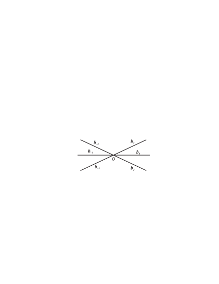
Figure 1: Star graph with six bonds.

II Nonlocal nonlinear Schrodinger equation on a line

PT-symmetric version of the nonlocal nonlinear Schrodinger equation on a line was proposed by Ablowitz and Muslimani in AM2013 and was studied later in different contexts, e.g., Refs.AM2014 -Panos2020 . Explicitly, NNLSE on a line can be written as

$$i\frac{\partial}{\partial t}q(x,t)=\frac{\partial^{2}}{\partial x^{2}}q(x,t)+2q^{2}(x,t)q^{*}(-x,t).$$ (1)

Eq.(1) can be rewritten as

$$\frac{\partial}{\partial t}q(x,t)=-i\frac{\partial^{2}}{\partial x^{2}}q(x,t)+iV(x,t),$$ (2)

where $V=-2q^{2}(x,t)q^{*}(-x,t)$ is the PT-symmetric self-induced potential. Eq.(2) describes the PT-symmetric optical solitons propagating in optical waveguide having ”gain-and-loss” structure. One-soliton solution of Eq.(1) can be obtained using the inverse scattering method and given as AM2013

$$q(x,t)=-\frac{2(\eta_{1}+\bar{\eta}_{1})e^{i\bar{\theta}_{1}}e^{-4i\bar{\eta}^{2}_{1}t}e^{-2\bar{\eta}_{1}x}}{1+e^{i(\theta_{1}+\bar{\theta}_{1})}+e^{4i(\eta^{2}_{1}-\bar{\eta}^{2}_{1})t}+e^{-2(\eta_{1}+\bar{\eta}_{1})x}}.$$ (3)

As it was stated in the Ref.AM2013 , solution given by Eq.(3) describes breathing soliton, whose center of mass oscillates around a fixed point. A bright (traveling) soliton solution was found in the RefStalin and can be written as

$$q(x,t)=\frac{\alpha e^{\bar{\xi}_{1}}}{1+e^{\xi_{1}+\bar{\xi}_{1}+\Delta}},$$ (4)

and the parity transformed complex conjugate solution

$$q^{*}(-x,t)=\frac{\beta e^{\xi_{1}}}{1+e^{\xi_{1}+\bar{\xi}_{1}+\Delta}},$$ (5)

where $\xi_{1}=ik_{1}x-ik_{1}^{2}t+\xi_{1}^{(0)},\,\bar{\xi}_{1}=i\bar{k}_{1}x-i\bar{k}_{1}^{2}t+\bar{\xi}_{1}^{(0)},\,e^{\Delta}=-\frac{\alpha\beta}{\kappa},\,\kappa=(k_{1}+\bar{k}_{1})^{2}$ and $k_{1},\bar{k}_{1},\alpha,\beta,\xi_{1}^{(0)},\bar{\xi}_{1}^{(0)}$ are arbitrary complex constants. Two conservative quantities (integrals of motion) can be determined for Eq.(1) as the norm:

$$C_{0}(t)=\underset{-\infty}{\overset{+\infty}{\int}}q(x,t)q^{*}(-x,t)dx.$$ (6)

and energy:

$$C_{2}(t)=\underset{-\infty}{\overset{+\infty}{\int}}\Big{[}\frac{\partial}{\partial x}q(x,t)\cdot\frac{\partial}{\partial x}q^{*}(-x,t)+$$

$$q^{2}(x,t)\cdot q^{*2}(-x,t)\Big{]}dx.$$ (7)

Integrability of Eq.(1) was proven in the Ref.AM2013 by showing existence of the infinite number of conserving quantities. In the next section we will extend the study of the Ref.AM2013 to the case one dimensional branched domains given in terms of the metric graphs.

III Extension to a star graph: Vertex boundary conditions and soliton solutions

Consider the following nonlocal nonlinear Schrödinger equation which is written on the each bond of the star graph with six semi-infinite bonds (see, Fig. 1) $b_{-j}\sim(-\infty;0]$ and $b_{j}\sim[0;+\infty),$

$$i\frac{\partial}{\partial t}q_{\pm j}(x,t)=\frac{\partial^{2}}{\partial x^{2}}q_{\pm j}(x,t)+\sqrt{\beta_{j}\beta_{-j}}q_{\pm j}^{2}(x,t)q_{\mp j}^{*}(-x,t),$$ (8)

where $q_{\pm j}(x,t)$ at $x\in b_{\pm j}$ and $j=1,2,3$.

Very important feature of Eq.(8) is the fact that it is a system of NLS equations, where components of $q_{j}$ are mixed in nonlinear term. Unlike classical NLSE on graphs, where components of solution are related to each other via the vertex boundary conditions, in Eq.(8), components with opposite signs are mixed via the nonlinear term, while other components are connected to each other via the vertex boundary conditions. To consider and solve Eq.(8), one needs to impose boundary conditions at the graph branching point (vertex). Such conditions can be derived from the fundamental conservation laws. Here we use norm and energy conservation to derive vertex boundary conditions.

For the above nonlocal NLSE, the norm determined as AM2013

$$C_{0}(t)=\underset{j=1}{\overset{3}{\sum}}\bigg{[}\underset{b_{j}}{\int}q_{j}(x,t)q_{-j}^{*}(-x,t)dx+$$

$$\underset{b_{-j}}{\int}q_{-j}(x,t)q_{j}^{*}(-x,t)dx\bigg{]}.$$ (9)

From the norm conservation, $\dot{C}_{0}=0$ we have

$$\sum_{j=1}^{3}\left.{\bf Im}\left[\frac{\partial}{\partial x}q_{j}(x,t)\cdot q_{-j}^{*}(-x,t)\right]\right|_{x\to+0}=$$

$$\sum_{j=1}^{3}\left.{\bf Im}\left[\frac{\partial}{\partial x}q_{-j}(x,t)\cdot q_{j}^{*}(-x,t)\right]\right|_{x\to-0}.$$ (10)

Another conserving quantity, i.e., the energy is given by

$$C_{2}(t)=\underset{j=1}{\overset{3}{\sum}}\Bigg{[}\underset{b_{j}}{\int}\left(\frac{\partial}{\partial x}q_{j}(x,t)\cdot\frac{\partial}{\partial x}q_{-j}^{*}(-x,t)-\frac{\sqrt{\beta_{j}\beta_{-j}}}{2}q_{j}^{2}(x,t)\cdot q_{-j}^{*2}(-x,t)\right)dx+$$

$$\underset{b_{-j}}{\int}\left(\frac{\partial}{\partial x}q_{-j}(x,t)\cdot\frac{\partial}{\partial x}q_{j}^{*}(-x,t)-\frac{\sqrt{\beta_{j}\beta_{-j}}}{2}q_{-j}^{2}(x,t)\cdot q_{j}^{*2}(-x,t)\right)dx\Bigg{]}.$$ (11)

The energy conservation, $\dot{C}_{2}=0$ leads to

$$\sum_{j=1}^{3}\left.{\bf Re}\left[\frac{\partial}{\partial t}q_{-j}^{*}(-x,t)\cdot\frac{\partial}{\partial x}q_{j}(x,t)\right]\right|_{x\to+0}=$$

$$\sum_{j=1}^{3}\left.{\bf Re}\left[\frac{\partial}{\partial t}q_{j}^{*}(-x,t)\cdot\frac{\partial}{\partial x}q_{-j}(x,t)\right]\right|_{x\to-0}.$$ (12)

Eqs. (10) and (12) are compatible with the following two sets of the vertex boundary conditions:

$$\alpha_{1}q_{1}(x,t)|_{x=0}=\alpha_{-1}q_{-1}(x,t)|_{x=0}=\alpha_{2}q_{2}(x,t)|_{x=0}=\alpha_{-2}q_{-2}(x,t)|_{x=0}=\alpha_{3}q_{3}(x,t)|_{x=0}=\alpha_{-3}q_{-3}(x,t)|_{x=0},$$

$$\left.\frac{1}{\alpha_{1}}\frac{\partial}{\partial x}q_{1}(x,t)\right|_{x=0}+\left.\frac{1}{\alpha_{2}}\frac{\partial}{\partial x}q_{2}(x,t)\right|_{x=0}+\left.\frac{1}{\alpha_{3}}\frac{\partial}{\partial x}q_{3}(x,t)\right|_{x=0}=$$

$$\left.\frac{1}{\alpha_{-1}}\frac{\partial}{\partial x}q_{-1}(x,t)\right|_{x=0}+\left.\frac{1}{\alpha_{-2}}\frac{\partial}{\partial x}q_{-2}(x,t)\right|_{x=0}+\left.\frac{1}{\alpha_{-3}}\frac{\partial}{\partial x}q_{-3}(x,t)\right|_{x=0}.$$ (13)

It should be noted that Eqs. (10) and (12) follow from the boundary conditions (13), but vice-versa is not true. Let $q(x,t)$ is the solution of nonlocal nonlinear Schrodinger equation given by

$$i\frac{\partial}{\partial t}q(x,t)=\frac{\partial^{2}}{\partial x^{2}}q(x,t)+2q^{2}(x,t)q^{*}(-x,t).$$ (14)

Then solution of Eq. (8) and (13) can be expressed in terms of $q(x,t)$ as $q_{\pm j}(x,t)=\sqrt{\frac{2}{\beta_{\pm j}}}q(x,t)$ and fulfills the boundary conditions (13), provided the following constraints hold true:

$$\frac{\alpha_{\pm j}}{\alpha_{1}}=\sqrt{\frac{\beta_{\pm j}}{\beta_{1}}},$$

$$\frac{1}{\beta_{1}}+\frac{1}{\beta_{2}}+\frac{1}{\beta_{3}}=\frac{1}{\beta_{-1}}+\frac{1}{\beta_{-2}}+\frac{1}{\beta_{-3}}.$$ (15)

One of explicit soliton solutions of Eq. (8) on a line have been obtained in the Ref. is AM2016 . Using this solution, corresponding soliton solution on a graph can be written as

$$q_{\pm j}(x,t)=-\sqrt{\frac{2}{\beta_{\pm j}}}\frac{4\eta e^{i\bar{\varphi}}e^{-4i\eta^{2}t}e^{-2\eta x}}{1+e^{i(\varphi+\bar{\varphi})}e^{-4\eta x}}.$$ (16)

$\varphi,\,\bar{\varphi},\,\eta$ are arbitrary complex constants.

IV Integrability of the problem

Here we will show integrability of the NNLSE on a metric star graph, given by Eqs.(8) and (13) by proving existence of the infinite number of conservation laws. This can be done following the prescription used for usual (not nonlocal) NLS on metric graphs in the Ref. Zarif . The soliton solutions of the problem on the infinite linear chain satisfy an infinite number of conservation laws given by

$$\underset{-\infty}{\overset{+\infty}{\int}}\mu_{n}[q(x,t),q^{*}(-x,t)]dx=C_{n},$$ (17)

where $C_{n}$ is a constant, $\mu_{n}$ is a polynomial of $q(x,t),\,q^{*}(-x,t)$ and their derivatives with respect to $x$ AM2016 . Using this relation, we now investigate the following quantities, which for are given on the metric star graph:

$$Q_{n}=\underset{j=1}{\overset{3}{\sum}}\bigg{[}\beta_{j}^{-1}\underset{b_{j}}{\int}\mu_{n}[q(x,t),q^{*}(-x,t)]dx+$$

$$\beta_{-j}^{-1}\underset{b_{-j}}{\int}\mu_{n}[q(x,t),q^{*}(-x,t)]dx\bigg{]},$$ (18)

where $q(x,t)$ the solution of Eq. (8) in the bonds $b_{\pm j}$ and $\mu_{n}[q(x,t),q^{*}(-x,t)]$ obeys the recursion relation

$$\mu_{n+1}=q\frac{\partial}{\partial x}\left(\frac{\mu_{n}}{q}\right)+\underset{m=0}{\overset{n-1}{\sum}}\mu_{m}\mu_{n-m-1},$$ (19)

$$\mu_{0}=q(x,t)q^{*}(-x,t),\,\mu_{1}=q(x,t)\partial_{x}q^{*}(-x,t).$$ (20)

Using Eq. (15), from the r.h.s. of Eq.(18) we can get

$$Q_{n}=(\beta_{-1}^{-1}+\beta_{-2}^{-1}+\beta_{-3}^{-1})\underset{-\infty}{\overset{0}{\int}}\mu_{n}[q(x,t),q^{*}(-x,t)]dx+$$

$$(\beta_{1}^{-1}+\beta_{2}^{-1}+\beta_{3}^{-1})\underset{0}{\overset{+\infty}{\int}}\mu_{n}[q(x,t),q^{*}(-x,t)]dx=$$

$$=(\beta_{1}^{-1}+\beta_{2}^{-1}+\beta_{3}^{-1})\underset{-\infty}{\overset{+\infty}{\int}}\mu_{n}[q(x,t),q^{*}(-x,t)]dx=$$

$$(\beta_{1}^{-1}+\beta_{2}^{-1}+\beta_{3}^{-1})C_{n}.$$ (21)

It is clear that due to the conservation law given by Eq.(17), $Q_{n}$ is constant, i.e. conserving quantity. Therefore, $Q_{n}$ is the constant of motion. This implies that nonlocal NLSE on metric star graph has infinite number of conservation laws and hence, integrable.

V Numerical results

It is clear that the above proven integrability of NNLSE (8) holds true for the case, when constraints given by Eq.(15) are fulfilled. Such integrable NLSE approves different soliton solutions, such as breathing given by Eq.(3) and traveling given by Eq.(4) solitons. For the case, when constraints in Eq.(15) are broken, one needs to solve Eq. (8) numerically as the initial value problem. As the initial conditions, we will choose values of exact (soliton) solutions at $t=0$. Discretization scheme from the Ref.AM2014 is used in numerical solutioin of Eq.(1). In Fig. 2 plots of $|q(x,t)|^{2}$ obtained by solving Eq.(8) numerically for the initial conditions imposed on the bond $b_{-1}$ and $b_{1}$ are presented for different time moments, $t=0\;\;0.05,\;\;0.1$ at the values of $\beta_{\pm j}$ fulfilling the sum rule in Eq. (15). A remarkable feature of the travelling solitons is the reflectionless transmission through the vertex. Fig. 3 presents similar plots for those values of $\beta_{\pm j}$, which do not fulfill the sum rule in (15). Unlike the solitons in Fig. 2, reflection at the vertex can be observed in this plot. Thus one can conclude that integrable case provides the reflectionless transmission of solitons through the branching point of the graph. —Earlier, such a feature was observed for other evolution equations on graphs, such as NLS Zarif , sine-Gordon Our1 and nonlinear Dirac KarimNLDE equations. The reason for such behavior of solitons described by the nonlinear Schrodinger equation on graphs, was explained in the Ref.Jambul1 .

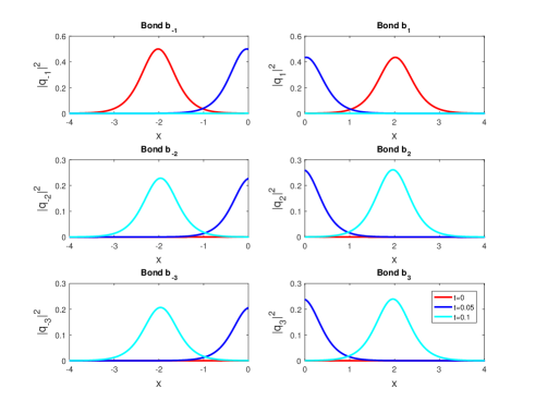
Figure 2: Plot of soliton on a metric star graph obtained from numerical solution of Eq.(8) for the values of $\beta_{j}$ fulfilling the sum rule in Eq.(8) ($\beta_{-1}=1$, $\beta_{1}=1.15$, $\beta_{-2}=2.19$, $\beta_{2}=1.91$, $\beta_{-3}=2.42$, $\beta_{3}=2.09$). The initial conditions are given on the bonds $b_{-1}$ and $b_{1}$.

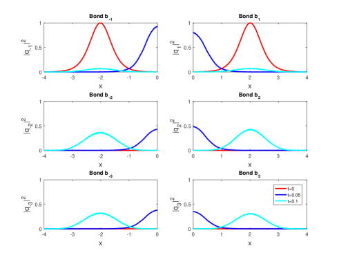
Figure 3: Plot of soliton on a metric star graph obtained from numerical solution of Eq.(8) for the values of $\beta_{j}$ breaking the sum rule in Eq.(8) ($\beta_{-1}=0.65$, $\beta_{1}=0.79$, $\beta_{-2}=2.7$, $\beta_{2}=2.09$, $\beta_{-3}=3.06$, $\beta_{3}=2.87$). The initial conditions are given on the bonds $b_{-1}$ and $b_{1}$.

VI Extension to a tree graph

The above treatment can be extended to the case other graphs. Here we will demonstrate that for a tree graph. One of possible tree graphs, on which one can write NNLSE, is presented in Fig.4. The central branch, i.e. the branch st the middle of the graph is chosen as an origin of coordinates. Then the bonds can be determined as $b_{-1},\;b_{-1mn}\sim(-\infty;0]$, $b_{-1m}\sim[-L_{1m};0]$, $b_{1m}\sim[0;L_{1m}]$, $b_{1},\;b_{1mn}\sim[0;+\infty)$, where $L_{1m}$ are the lengths of $b_{\pm 1m}$ bonds and $m=1,2$, $n=1,2$. Here the ”+” sign is for right-handed bonds and the ”-” sign is for left-handed bonds from the center of the tree graph.

On each bond of such graph one can write nonlocal nonlinear Schrodinger equation given be Eq.(8) with $j=\pm 1,\;\pm 1m,\;\pm 1mn$.

The vertex boundary conditions following from the conservation laws are given as

$$\alpha_{\pm 1}q_{\pm 1}(x,t)|_{x=0}=\alpha_{\mp 11}q_{\mp 11}(x,t)|_{x=0}=\alpha_{\mp 12}q_{\mp 12}(x,t)|_{x=0},$$

$$\left.\frac{1}{\alpha_{\pm 1}}\frac{\partial}{\partial x}q_{\pm 1}(x,t)\right|_{x=0}=\left.\frac{1}{\alpha_{\mp 11}}\frac{\partial}{\partial x}q_{\mp 11}(x,t)\right|_{x=0}+$$

$$\left.\frac{1}{\alpha_{\mp 12}}\frac{\partial}{\partial x}q_{\mp 12}(x,t)\right|_{x=0},$$ (22)

$$\alpha_{\pm 1m}q_{\pm 1m}(x,t)|_{x=\pm L_{1m}}=\alpha_{\pm 1m1}\lim_{x\to\pm 0}q_{\pm 1m1}(x,t)=$$

$$\alpha_{\pm 1m2}\lim_{x\to\pm 0}q_{\pm 1m2}(x,t),$$

$$\left.\frac{1}{\alpha_{\pm 1m}}\frac{\partial}{\partial x}q_{\pm 1m}(x,t)\right|_{x=\pm L_{1m}}=\frac{1}{\alpha_{\pm 1m1}}\lim_{x\to\pm 0}\frac{\partial}{\partial x}q_{\pm 1m1}(x,t)+$$

$$\frac{1}{\alpha_{\pm 1m2}}\lim_{x\to\pm 0}\frac{\partial}{\partial x}q_{\pm 1m2}(x,t).$$ (23)

Assuming that the following sum rules hold true:

$$\frac{\alpha_{\pm 1}}{\sqrt{\beta_{\pm 1}}}=\frac{\alpha_{\pm 11}}{\sqrt{\beta_{\pm 11}}}=\frac{\alpha_{\pm 12}}{\sqrt{\beta_{\pm 12}}},$$

$$\frac{1}{\alpha_{\pm 1}\sqrt{\beta_{\pm 1}}}=\frac{1}{\alpha_{\pm 11}\sqrt{\beta_{\pm 11}}}+\frac{1}{\alpha_{\pm 12}\sqrt{\beta_{\pm 12}}},$$

$$\frac{1}{\beta_{\pm 1}}=\frac{1}{\beta_{\pm 11}}+\frac{1}{\beta_{\pm 12}}.$$ (24)

$$\frac{\alpha_{\pm 1m}}{\sqrt{\beta_{\pm 1m}}}=\frac{\alpha_{\pm 1m1}}{\sqrt{\beta_{\pm 1m1}}}=\frac{\alpha_{\pm 1m2}}{\sqrt{\beta_{\pm 1m2}}},$$

$$\frac{1}{\alpha_{\pm 1m}\sqrt{\beta_{\pm 1m}}}=\frac{1}{\alpha_{\pm 1m1}\sqrt{\beta_{\pm 1m1}}}+\frac{1}{\alpha_{\pm 1m2}\sqrt{\beta_{\pm 1m2}}},$$

$$\frac{1}{\beta_{\pm 1m}}=\frac{1}{\beta_{\pm 1m1}}+\frac{1}{\beta_{\pm 1m2}},$$ (25)

the soliton solutions on each bond can be written as

$$q_{\pm 1}(x,t)=\sqrt{\frac{2}{\beta_{\pm 1}}}q(x+S_{\pm 1},t),$$

$$q_{\pm 1m}(x,t)=\sqrt{\frac{2}{\beta_{\pm 1m}}}q(x+S_{\pm 1m},t),$$

$$q_{\pm 1mn}(x,t)=\sqrt{\frac{2}{\beta_{\pm 1mn}}}q(x+S_{\pm 1mn},t),$$ (26)

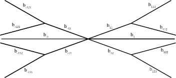
Figure 4: A sketch of tree graph adopted for nonlocal nonlinear Schrodinger equation

where $S_{\pm 1}=S_{\pm 1m}=x_{0}$, $S_{\pm 1mn}=\pm L_{1m}+x_{0}$, $x_{0}$ is the coordinate of the center of soliton at $t=0$. Integrability of nonlocal nonlinear Schrodinger on tree graph presented in Fig.4 equation (for the case, when the above sum rules are fulfilled) can be shown similarly to that for the star graph. Also, one can show by numerical computations that for the integrable case transmission of nonlocal PT-symmetric solitons are reflectionless. We note that the above treatment can be directly extended to other graph topologies, provided a graph consist of even number number of bonds symmetrically positioned with respect to the origin of coordinates, i.e., one has equal number of bonds on each side of the origin of coordinates. In addition, at least four bonds of the graph should be semi-infinite. Unlike the solution of usual nonlinear Schrodinger equation on graphs, solution of PT-symmetric nonlocal nonlinear NLSE on graphs is much complicated that makes the dynamics of nonlocal solitons more rich than that for usual soliton. The latter implies also existence of more tools for tuning the soliton dynamics.

VII Conclusions

In this paper we studied dynamics of solitons described by PT-symmetric nonlocal nonlinear Schrodinger equation on networks by modeling these latter in terms of metric graphs. Integrability of the problem in case of fulfilling certain constraints given in terms of nonlinearity coefficients is shown. Exact soliton solutions which are valid for this case are obtained. For the case, when the constraints are broken, the problem is solved numerically. The analysis of soliton dynamics shows absence of the back scattering in the transmission of soliton through the graph node, is sum rule in Eq. (15) is fulfilled. When this sum rule is broken, the transmission is accompanied by scattering of solitons at the node. The treatment is extended for tree graph and possibility for extension for other complicated graphs is discussed. The above model can be applied for describing the soliton dynamics in optical fiber network, where each branch has self-induced gain-loss and other branched waveguides generating self-induced PT-symmetric potential.

References

• (1) M.J. Ablowitz, Z.H. Musslimani, Phys. Rev. Lett. 110, 064105 (2013).
• (2) M.J. Ablowitz, Z.H. Musslimani, M.J. Ablowitz, Z.H. Musslimani, Phys. Rev. Lett. 110, 064105 (2013).
• (3) M.J. Ablowitz, Z.H. Musslimani, Nonlinearity 29, 915 (2016).
• (4) M.J. Ablowitz, Z.H. Musslimani, Stud. Appl. Math. 139, 7 (2016).
• (5) D. Sinha, P. K. Ghosh, Rev. E 91, 042908 (2018).
• (6) J. Yang, Phys. Rev. E 98, 042202 (2018).
• (7) S.Stalin, M.Senthilvelan, M.Lakshmanan, Phys.Lett. A, 377, 860 (2017).
• (8) Z. Wen, Zh. Yan, CHAOS, 27, 053105 (2017).
• (9) B-F. Feng, X-D. Luo, M. J. Ablowitz and Z. H. Musslimani, Nonlinearity 31, 5385 (2018).
• (10) M. J. Ablowitz, X-D. Luo and Z. H. Musslimani, J. Math.Phys. 59, 011501 (2018).
• (11) M.J. Ablowitz, Z.H. Musslimani, J. Phys. A. 52, 15LT02 (2019).
• (12) J. Yang,Phys.Rev.E 98, 042202 (2018).
• (13) J. Rao, J. He, T. Kanna, and D. Mihalache, Phys. Rev. E, 102, 032201 (2020).
• (14) C. B. Ward, P. G. Kevrekidis, T. P. Horikis, and D. J. Frantzeskakis, Phys. Rev. Research, 2, 013351 (2020).
• (15) V. V. Konotop, J. Yang, D. A. Zezyulin, Rev., Mod. Phys. 88, 035002 (2016).
• (16) H. Susanto, S. van Gils, A. Doelman, and G. Derks, Physica C. 408, 579 (2004).
• (17) H. Susanto, S. van Gils, A. Doelman, and G. Derks, Phys. Rev. B 69, 212503 (2004).
• (18) Z.Sobirov, D.Matrasulov, K.Sabirov, S.Sawada, and K.Nakamura, Phys. Rev. E 81 , 066602 (2010).
• (19) Z. Sobirov, D. Matrasulov, S. Sawada, and K. Nakamura, Phys.Rev.E 84, 026609 (2011).
• (20) R.Adami, C.Cacciapuoti, D.Finco, D.Noja, Rev.Math.Phys, 23 4 (2011).,
• (21) K.K.Sabirov, Z.A.Sobirov, D.Babajanov, and D.U.Matrasulov, Phys.Lett. A, 377, 860 (2013).
• (22) D.Noja, Philos. Trans. R. Soc. A 372, 20130002 (2014).
• (23) H.Uecker, D.Grieser, Z.Sobirov, D.Babajanov and D.Matrasulov, Phys. Rev. E 91, 023209 (2015).
• (24) D.Noja, D.Pelinovsky, and G.Shaikhova, Nonlinearity 28, 2343 (2015).
• (25) R.Adami, C.Cacciapuoti, D.Noja, J. Diff. Eq., 260 7397 (2016).
• (26) V. Caudrelier, Comm. Math. Phys. 338 893 (2015).
• (27) Z.Sobirov, D.Babajanov, D.Matrasulov, K.Nakamura, and H.Uecker, EPL 115 , 50002 (2016).
• (28) R Adami, E Serra, P Tilli, Commun. Math. Phys., 352, 387 (2017).
• (29) A. Kairzhan, D.E. Pelinovsky, J. Phys. A: Math. Theor. 51, 095203 (2018).
• (30) K.K.Sabirov, S. Rakhmanov, D. Matrasulov and H. Susanto, Phys.Lett. A, 382, 1092 (2018).
• (31) K.K.Sabirov, J.Yusupov, D. Jumanazarov, D. Matrasulov, Phys.Lett. A, 382, 2856 (2018).
• (32) K.K. Sabirov, D.B. Babajanov, D.U. Matrasulov and P.G. Kevrekidis, J. Phys. A: Math. Theor. 51 435203 (2018).
• (33) D. Babajanov, H. Matyoqubov and D. Matrasulov, J. Chem. Phys.,149, 164908 (2018).
• (34) D.U. Matrasulov, J.R. Yusupov and K.K. Sabirov, J. Phys. A, 52, 155302 (2019).
• (35) J.R. Yusupov, K.K. Sabirov, M. Ehrhardt and D.U. Matrasulov, Phys. Lett. A, 383, 2382 (2019).
• (36) J.R. Yusupov, K.K. Sabirov, M. Ehrhardt and D.U. Matrasulov, Phys. Rev. E, 100, 032204 (2019).
• (37) J.R. Yusupov, Kh.Sh. Matyokubov, K.K. Sabirov and D.U. Matrasulov, Chem. Phys., 537, 110861 (2020).
• (38) D. Matrasulov, K. Sabirov, D. Babajanov, H. Susanto, EPL, 130 67002 (2020).
• (39) K.K. Sabirov, M.E. Akramov, R. Sh. Otajonov, D.U. Matrasulov, Chaos, Solitons $\&$ Fractals, 133 109636 (2020).
• (40) K.K. Sabirov, J.R. Yusupov, D.U. Matrasulov, ArXiv:2011.02278
• (41) K. K. Sabirov, J. R. Yusupov, M. M. Aripov, M. Ehrhardt, and D. U. Matrasulov, Phys. Rev. E 103, 043305 (2021).