Multi-breather solutions to the Sasa-Satsuma equation

Abstract

General breather solution to the Sasa-Satsuma (SS) equation is systematically investigated in this paper. We firstly transform the SS equation into a set of three Hirota bilinear equations under proper plane wave background. Starting from a specially arranged tau-function of the Kadomtsev-Petviashvili hierarchy and a set of eleven bilinear equations satisfied, we implement a series steps of reduction procedure, i.e., C-type reduction, dimension reduction and complex conjugate reduction, and reduce these eleven equations to three bilinear equations for the SS equation. Meanwhile, general breather solution to the SS equation is found in determinant of even order. The one- and two-breather solutions are calculated and analyzed in details.

 
*Corresponding author. Email address: baofeng.feng@utrgv.edu.

1 Introduction

Breathers are ubiquitous phenomena in many physical systems either in continuous or discrete ones. It is a particular type of nonlinear wave whose energy is localized in space but oscillates over time, or vice versa. The exactly solvable sine-Gordon equation [1] and the focusing nonlinear Schrödinger equation [2] are examples of one-dimensional partial differential equations that possess breather solutions [3].

The so-called intrinsic localized modes (ILMs) or the discrete breathers (DBs) in Fermi-Pasta-Ulam (FPU) lattices were reported in the late 1980s [4, 5]. They have been recently observed experimentally in various physical contexts such as coupled optical waveguides [6, 7], Josephson junction ladders [8, 9], antiferromagnet crystals [10], and micromechanical oscillator arrays [11].

Breathers have met with success in understanding the final stage of a certain nonlinear process that is initiated from modulation instability (MI, also known as the Benjamin-Feir instability) [12]. It is well-known that MI is one of the most ubiquitous phenomena in nature and commonly appears in many physical contexts such as water waves, plasma waves and electromagnetic transmission lines [13]. Whereas recent theoretical developments indicated that the presence of baseband MI supports the generation of rogue waves (RW) [14], breathers also appear to be a significant strategy in deriving RW solutions of many integrable equations [16, 15].

The nonlinear Schrödinger equation (NLSE)

$$\mathbf{i}\frac{\partial q}{\partial T}+\frac{1}{2}\frac{\partial^{2}q}{\partial X^{2}}\pm|q|^{2}q=0$$ (1)

describes the evolution of weakly nonlinear and quasi-monochromatic waves in dispersive media [17]. This equation has found applications in numerous areas of physics, ranging from nonlinear optical fibers [18], plasma physics [19] to Bose-Einstein condensates [20]. From the mathematical point of view, the NLSE is considered to be a fundamental model in investigating breather and RW solutions [21, 22, 23]. In particular, the Akhmediev breather (AB) [21] and Kuznetsov-Ma soliton (KM) [24, 25], where AB (KM) is periodic in space (time) and localized in time (space), have captured wide attention. Remarkably, when we take the large-period limits, both of them degenerate to the Peregrine soliton [26], which is localized both in time and space and turns into a prototype of RWs. It turns out that this idea has been widely adopted in constructing RW solutions of many other integrable equations and their multi-component generalizations [15, 27].

The NLSE is one of the most fundamental integrable equations in the sense that it only incorporates the lowest-order dispersion and the lowest-order nonlinear term. However, higher-order terms are indispensable in more complicated circumstances, such as modeling the ultrashort pulses generated due to the MI [28] and examing the one-dimensional Heisenberg spin chain [29]. As such, a number of integrable extensions of the NLSE have been proposed, including the higher-order NLSE [18], the Sasa-Satsuma equation [30, 31] and the Kundu-NLSE [32], to name a few examples. Therefore it is natural to expand the investigations on NLSE to these integrable models. While compared with the NLSE it is more challenging to obtain soliton, breather, or RW solutions of these equations [33, 34, 35, 36], the occurrence of higher-order terms may also induce various new features to the solutions and enrich the solution dynamics [16].

As mentioned above, the Sasa-Satsuma equation (SSE) is a nontrivial integrable extension of the NLSE and can be written in the form [30]

$$\mathbf{i}\frac{\partial q}{\partial T}+\frac{1}{2}\frac{\partial^{2}q}{\partial X^{2}}+|q|^{2}q+\mathbf{i}\varepsilon\left\{\frac{\partial^{3}q}{\partial X^{3}}+6|q|^{2}\frac{\partial q}{\partial X}+3q\frac{\partial|q|^{2}}{\partial X}\right\}=0,$$ (2)

where $q$ corresponds to the complex envelope of the wave field and the real constant $\varepsilon$ scales the integrable perturbations of the NLSE. For $\varepsilon=0$, the SSE reduces to the NLSE. As an extension of the NLSE, the SSE consists of terms describing the third-order dispersion, the self-steepening and the self-frequency shift that are commonly involved in nonlinear optics [37, 38]. For the convenience of analyzing the SSE, according to the work of Sasa and Satsuma [30], one can introduce the transformation

$$u(x,t)=q(X,T)\exp\left\{-\frac{\mathbf{i}}{6\varepsilon}\left(X-\frac{T}{18\varepsilon}\right)\right\},$$ (3)

where $t=T$ and $x=X-T/(12\varepsilon)$, then the equation (2) is transformed into

$$u_{t}+\varepsilon(u_{xxx}+6|u|^{2}u_{x}+3u(|u|^{2})_{x})=0.$$ (4)

On account of its integrability and physical implications, the SSE has attracted much attention since it was discovered. For instance, the double hump soliton solution of the SSE was obtained by Mihalache et al. [34] while its multisoliton solutions have been constructed in the Refs.[35, 39] by the Kadomtsev-Petviashvili (KP) hierarchy reduction method. In addition to the soliton solutions, RW solutions [40, 42, 41, 43] of the SSE have also been found via the method of Darboux transformation [27], and in contrast to the NLSE, several intriguing solution structures were reported like the so-called twisted RW pair [40]. Beyond that, the long-time asymptotic behaviour of the SSE with decaying initial data was analyzed in [44] by formulating the Riemann-Hilbert problem.

Despite extensive investigations on the SSE, its breather solutions have not been systematically examined, to the best of our knowledge. Consequently, the main objective of this paper is to derive multi-breather solutions to the Sasa-Satsuma equation

$$u_{t}=u_{xxx}-6c|u|^{2}u_{x}-3cu\left(|u|^{2}\right)_{x},$$ (5)

where $c$ is a real constant. The rest of this paper is organized as follows. In Section 2, general multi-breather solutions of equation (5) are presented in Theorem 2.1. The detailed derivations of these solutions are provided in Section 3. In this process, we firstly transform the equation (5) into bilinear forms. Then multi-breather solutions of equation (5) can be obtained by relating the bilinear forms of (5) with a set of eleven bilinear equations in the KP hierarchy. Although the idea seems to be straightforward, the intermediate computations are extremely complicated due to the complexity of the SSE and multiple corresponding bilinear equations from the KP hierarchy. In addition to the dimension reduction and the complex conjugate reduction, which are the common obstructions in applying the KP hierarchy reduction method [22, 45, 47, 46, 48, 49], a new obstacle is to tackle the symmetry reduction (44). As pointed out in [35], when applying the direct method [50] to find soliton solutions, one only needs to truncate at power two of the formal expansion for NLSE whereas one has to go to power four for SSE, thereby resulting in more sophisticated analysis. It turns out that this also appears in our consideration, namely the structure of breather solutions of SSE is more intricate than that of NLSE (see Theorem 2.1). In Section 4, the solution dynamics are discussed in detail. Six types of first-order breathers were found totally and various configurations of second- and third-order breathers have been illustrated. The main results of this paper are summarized in Section 5.

2 Multi-breather solutions to the Sasa-Satsuma equation

In this section, we present the multi-breather solutions to the Sasa-Satsuma equation (5).

Theorem 2.1.

The Sasa-Satsuma equation (5) admits the multi-breather solution

$$u=\frac{g}{f}e^{\mathrm{i}\left(\kappa(x-6ct)-\kappa^{3}t\right)}$$ (6)

where $\kappa$ is real,

$$f(x,t)=\tau_{0}(x-6ct,t),\quad g(x,t)=\tau_{1}(x-6ct,t)$$

and $\tau_{k}\,(k=0,1)$ is defined as

$$\tau_{k}=\left|\sum_{m,n=1}^{2}\frac{1}{p_{im}+p_{jn}}\left(-\frac{p_{im}-a}{p_{jn}+a}\right)^{k}e^{\xi_{im}+\xi_{jn}}\right|_{2N\times 2N}.$$ (7)

Here, $a=\mathbf{i}\kappa$ is purely imaginary, $\xi_{im}=p_{im}x+p_{im}^{3}t+\xi_{im,0}$, $N$ is a positive integer and the parameters $\xi_{im,0},p_{im}\,(i=1,\cdots,2N,m=1,2)$ satisfy the constraints

$$\left(p_{i1}^{2}+\kappa^{2}\right)\left(p_{i2}^{2}+\kappa^{2}\right) = -2c\left(p_{i1}p_{i2}-\kappa^{2}\right)$$ (8)

and

$$p_{N+l,m}=p_{lm}^{*},\quad\xi_{N+l,m,0}=\xi_{lm,0}^{*},\quad l=1,\cdots,N,$$ (9)

where $*$ denotes complex conjugation.

Remark.

We note that the parameter relations (8) and (9) presented in Theorem 2.1 give rise to $6N+1$ free real parameters which include $\kappa$, the real parts and imaginary parts of $p_{i1}$ and $\xi_{im,0},i=1,\cdots,N,m=1,2$.

Remark.

For $c=-4\kappa^{2}$, we can solve the equation (8) for $p_{i2}$ that is given by

$$p_{i2}=\frac{4\kappa^{2}p_{i1}\pm\mathbf{i}\kappa\left(p_{i1}^{2}-3\kappa^{2}\right)}{\kappa^{2}+p_{i1}^{2}}.$$

When $c\not=-4\kappa^{2}$, the expression of $p_{i2}$ is more complicated. If we set $p_{i1}=P_{\text{R}}+\mathbf{i}P_{\text{I}}$, where $P_{R}$ and $P_{I}$ represent the real and imaginary parts of $p_{i1}$ respectively, then $p_{i2}$ can be expressed as

$$p_{i2} = \frac{G+\mathbf{i}H}{K}$$

where

$$G = -P_{I}^{2}\left(\pm\alpha+2cP_{R}\right)+\left(\kappa^{2}+P_{R}^{2}\right)\left(\pm\alpha-2cP_{R}\right)$$

$$H = \left(\kappa^{2}-P_{I}^{2}\right)\left(\pm\beta-2cP_{I}\right)+P_{R}^{2}\left(\pm\beta+2cP_{I}\right)\mp 2\alpha P_{I}P_{R}$$

$$K = 2\left[2P_{I}^{2}\left(P_{R}^{2}-\kappa^{2}\right)+P_{I}^{4}+\left(\kappa^{2}+P_{R}^{2}\right){}^{2}\right]$$

with

$$\alpha = \sqrt[4]{X^{2}+Y^{2}}\cos\theta$$

$$\beta = \sqrt[4]{X^{2}+Y^{2}}\sin\theta$$

$$X = -4\left[P_{I}^{2}\left(c^{2}+2c\kappa^{2}+\kappa^{2}P_{I}^{2}-2\kappa^{4}\right)-P_{R}^{2}\left(c^{2}+2c\kappa^{2}+6\kappa^{2}P_{I}^{2}-2\kappa^{4}\right)-2c\kappa^{4}+\kappa^{6}+\kappa^{2}P_{R}^{4}\right]$$

$$Y = 8P_{I}P_{R}\left[c^{2}+2c\kappa^{2}+2\kappa^{2}\left(P_{I}^{2}-P_{R}^{2}\right)-2\kappa^{4}\right]$$

$$\theta = \arctan(Y/X)/2.$$

3 Derivation of the multi-breather solutions

This section is devoted to the construction of multi-breather solutions to the Sasa-Satsuma equation (5). It consists of two main steps. First, we transform the Sasa-Satsuma equation (5) into bilinear forms. Then multi-breather solutions are derived by showing that such bilinear equations can be obtained from reductions of the KP hierarchy.

3.1 Bilinear forms of the Sasa-Satsuma equation

The bilinearization of the Sasa-Satsuma equation (5) is established by the proposition below.

Proposition 3.1.

The Sasa-Satsuma equation

$$u_{t}=u_{xxx}-6c|u|^{2}u_{x}-3cu\left(|u|^{2}\right)_{x}$$

can be transformed into the system of bilinear equations

$$\left(D_{x}^{2}-4c\right)f\cdot f=-4cgg^{*}$$ (10)

$$\left(D_{x}^{3}-D_{t}+3\mathrm{i}\kappa D_{x}^{2}-3\left(\kappa^{2}+4c\right)D_{x}-6\mathrm{i}\kappa c\right)g\cdot f+6\mathrm{i}\kappa cqg=0$$

$$\left(D_{x}+2\mathrm{i}\kappa\right)g\cdot g^{*}=2\mathrm{i}\kappa qf$$

by the variable transformation

$$u=\frac{g}{f}e^{\mathrm{i}\left(\kappa(x-6ct)-\kappa^{3}t\right)},$$ (11)

where $\kappa$ is real, $f$ is a real-valued function, $g$ is a complex-valued function, $q$ is an auxiliary function and $D$ is the Hirota’s bilinear operator [50] defined by

$$D_{x}^{m}D_{t}^{n}f\cdot g=\left.\left(\frac{\partial}{\partial x}-\frac{\partial}{\partial{x^{\prime}}}\right)^{m}\left(\frac{\partial}{\partial t}-\frac{\partial}{\partial{t^{\prime}}}\right)^{n}[f(x,t)g(x^{\prime},t^{\prime})]\right|_{x^{\prime}=x,t^{\prime}=t}.$$

Proof.

By substituting (11) into equation (5) and rewriting the resulting equation in bilinear forms, we obtain

$$-f^{2}D_{t}g\cdot f+f^{2}D_{x}^{3}g\cdot f-3\left(D_{x}g\cdot f\right)\left(D_{x}^{2}f\cdot f\right)+3\mathbf{i}\kappa f^{2}\left(D_{x}^{2}g\cdot f\right)$$ (12)

$$-3\mathbf{i}\kappa fg\left(D_{x}^{2}f\cdot f\right)-3\kappa^{2}f^{2}\left(D_{x}g\cdot f\right)-c\left(9gg^{*}D_{x}g\cdot f+3g^{2}D_{x}g^{*}\cdot f\right)$$

$$-c\left(-6\mathbf{i}\kappa gf^{3}+6\mathbf{i}\kappa fg^{2}g^{*}\right)=0.$$

Apply the following identity to the equation above

$$9gg^{*}D_{x}g\cdot f+3g^{2}D_{x}g^{*}\cdot f=-3gf(D_{x}g\cdot g^{*})+12gg^{*}(D_{x}g\cdot f),$$ (13)

then (12) can be rearranged as

$$f^{2}[(D_{x}^{3}-D_{t}+3\mathbf{i}\kappa D_{x}^{2}-3(\kappa^{2}+4c)D_{x}+6\mathbf{i}c\kappa)g\cdot f]+3cgf[(D_{x}-2\mathbf{i}\kappa)g\cdot g^{*}]$$

$$-3(D_{x}g\cdot f)[(D_{x}^{2}-4c)f\cdot f+4cgg^{*}]-3\mathbf{i}\kappa fg(D_{x}^{2}f\cdot f)=0.$$ (14)

If we require

$$(D_{x}^{2}-4c)f\cdot f+4cgg^{*}=0,$$ (15)

then equation (14) reduces to

$$f^{2}[(D_{x}^{3}-D_{t}+3\mathbf{i}\kappa D_{x}^{2}-3(\kappa^{2}+4c)D_{x}-6\mathbf{i}c\kappa)g\cdot f]+3cgf[(D_{x}+2\mathbf{i}\kappa)g\cdot g^{*}]=0,$$ (16)

which can be decomposed as

$$\begin{cases}(D_{x}^{3}-D_{t}+3\mathbf{i}\kappa D_{x}^{2}-3(\kappa^{2}+4c)D_{x}-6\mathbf{i}c\kappa)g\cdot f=-6\mathrm{i}\kappa cqg\\ (D_{x}+2\mathbf{i}\kappa)g\cdot g^{*}=2\mathbf{i}\kappa qf\end{cases}$$ (17)

where $q$ is an auxiliary function. As a consequence, combing the equations (15) and (17) shows that the Sasa-Satsuma equation (5) can be transformed into the system of bilinear equations (10) via the transformation (11). ∎

3.2 Derivation of multi-breather solutions

In order to derive multi-breather solutions of the Sasa-Satsuma equation (5), we first present a crucial lemma.

Lemma 3.2.

The bilinear equations in the KP hierarchy

$$(D_{r}D_{x}-2)\tau_{kl}\cdot\tau_{kl}=-2\tau_{k+1,l}\tau_{k-1,l}$$ (18)

$$(D_{s}D_{x}-2)\tau_{kl}\cdot\tau_{kl}=-2\tau_{k,l+1}\tau_{k,l-1}$$ (19)

$$(D_{x}^{2}-D_{y}+2aD_{x})\tau_{k+1,l}\cdot\tau_{kl}=0$$ (20)

$$(D_{x}^{2}-D_{y}+2bD_{x})\tau_{k,l+1}\cdot\tau_{kl}=0$$ (21)

$$\left(D_{x}^{3}+3D_{x}D_{y}-4D_{t}+3a\left(D_{x}^{2}+D_{y}\right)+6a^{2}D_{x}\right)\tau_{k+1,l}\cdot\tau_{kl}=0$$ (22)

$$\left(D_{x}^{3}+3D_{x}D_{y}-4D_{t}+3b\left(D_{x}^{2}+D_{y}\right)+6b^{2}D_{x}\right)\tau_{k,l+1}\cdot\tau_{kl}=0$$ (23)

$$\left(D_{r}\left(D_{x}^{2}-D_{y}+2aD_{x}\right)-4D_{x}\right)\tau_{k+1,l}\cdot\tau_{kl}=0$$ (24)

$$\left(D_{s}\left(D_{x}^{2}-D_{y}+2bD_{x}\right)-4D_{x}\right)\tau_{k,l+1}\cdot\tau_{kl}=0$$ (25)

$$\left(D_{s}\left(D_{x}^{2}-D_{y}+2aD_{x}\right)-4\left(D_{x}+a-b\right)\right)\tau_{k+1,l}\cdot\tau_{kl}+4(a-b)\tau_{k+1,l+1}\tau_{k,l-1}=0\color[rgb]{1,1,1}{aaaaa}$$ (26)

$$\left(D_{r}\left(D_{x}^{2}-D_{y}+2bD_{x}\right)-4\left(D_{x}+b-a\right)\right)\tau_{k,l+1}\cdot\tau_{kl}+4(b-a)\tau_{k+1,l+1}\tau_{k-1,l}=0\color[rgb]{1,1,1}{aaaaa}$$ (27)

$$\left(D_{x}+a-b\right)\tau_{k+1,l}\cdot\tau_{k,l+1}=(a-b)\tau_{k+1,l+1}\tau_{kl}$$ (28)

admit the $M\times M$ Gram-type determinant solutions

$$\tau_{kl}=\left|m_{ij}^{kl}\right|_{M\times M}$$ (29)

where

$$m_{ij}^{kl} = \int\left(\sum_{m=1}^{2}\phi_{im}^{k,l}\right)\left(\sum_{n=1}^{2}\bar{\phi}_{jn}^{k,l}\right)dx$$ (30)

$$= \sum_{m,n=1}^{2}\frac{1}{p_{im}+q_{jn}}\left(\frac{a-p_{im}}{a+q_{jn}}\right)^{k}\left(\frac{b-p_{im}}{b+q_{jn}}\right)^{l}e^{\xi_{im}+\bar{\xi}_{jn}}$$ (31)

$$\phi_{im}^{k,l} = \left(p_{im}-a\right)^{k}\left(p_{im}-b\right)^{l}e^{\xi_{im}}$$ (32)

$$\bar{\phi}_{jn}^{k,l} = (-1)^{k}\left(q_{jn}+a\right)^{-k}(-1)^{l}\left(q_{jn}+b\right)^{-l}e^{\bar{\xi}_{jn}}$$ (33)

with

$$\xi_{im} = p_{im}x+p_{im}^{2}y+p_{im}^{3}t+\frac{1}{p_{im}-a}r+\frac{1}{p_{im}-b}s+\xi_{im,0}$$ (34)

$$\bar{\xi}_{jn} = q_{jn}x-q_{jn}^{2}y+q_{jn}^{3}t+\frac{1}{q_{jn}+a}r+\frac{1}{q_{jn}+b}s+\eta_{jn,0}.$$ (35)

Here, $p_{im},q_{jn},\xi_{im,0},\eta_{jn,0}\,(i,j=1,\cdots M,m,n=1,2),a$ and $b$ are complex constants while $k$ and $l$ are integers.

In what follows, we will establish the reductions from the bilinear equations (18)-(28) in the KP hierarchy to the bilinear equations (10), which consist of several steps. Once this is accomplished, multi-breather solutions of the Sasa-Satsuma equation (5) will be derived. We start with the reduction from AKP to CKP [51]. To this end, we take

$$q_{j1}=p_{j1},\quad q_{j2}=p_{j2},\quad b=-a,\quad\xi_{jn,0}=\eta_{jn,0}$$

where $j=1,\cdots M$ and $n=1,2$, then we obtain

$$\xi_{jn}(x,y,t,r,s)=\bar{\xi}_{jn}(x,-y,t,s,r).$$

Therefore, we have

$$m_{ji}^{-l,-k}(x,-y,t,s,r) = \sum_{m,n=1}^{2}\frac{1}{p_{jm}+q_{in}}\left(\frac{a-p_{jm}}{a+q_{in}}\right)^{-l}\left(\frac{b-p_{jm}}{b+q_{in}}\right)^{-k}e^{(\xi_{jm}+\bar{\xi}_{in})(x,-y,t,s,r)}$$

$$= \sum_{m,n=1}^{2}\frac{1}{p_{jm}+p_{in}}\left(\frac{a-p_{jm}}{a+p_{in}}\right)^{-l}\left(\frac{a+p_{jm}}{a-p_{in}}\right)^{-k}e^{\xi_{in}+\bar{\xi}_{jm}}$$

$$= \sum_{m,n=1}^{2}\frac{1}{p_{jm}+p_{in}}\left(\frac{a-p_{in}}{a+p_{jm}}\right)^{k}\left(\frac{a+p_{in}}{a-p_{jm}}\right)^{l}e^{\xi_{in}+\bar{\xi}_{jm}}$$

$$= \sum_{m,n=1}^{2}\frac{1}{p_{im}+p_{jn}}\left(\frac{a-p_{im}}{a+p_{jn}}\right)^{k}\left(\frac{a+p_{im}}{a-p_{jn}}\right)^{l}e^{\xi_{im}+\bar{\xi}_{jn}}$$

$$= m_{ij}^{kl}(x,y,t,r,s)$$

and

$$\tau_{kl}(x,y,t,r,s)=\tau_{-l,-k}(x,-y,t,s,r).$$ (36)

Next, we perform the dimension reduction. First, we rewrite $\tau_{kl}$ as

$$\tau_{kl}=\prod_{i=1}^{M}e^{\xi_{i2}+\bar{\xi}_{i2}}\widetilde{\tau}_{kl}$$

where

$$\widetilde{\tau}_{kl}=\left|\widetilde{m}_{ij}^{kl}\right|$$

and

$$\widetilde{m}_{ij}^{kl} = F_{kl}(p_{i1},p_{j1})e^{\xi_{i1}-\xi_{i2}+\bar{\xi}_{j1}-\bar{\xi}_{j2}}+F_{kl}(p_{i1},p_{j2})e^{\xi_{i1}-\xi_{i2}}$$ (38)

$$+F_{kl}(p_{i2},p_{j1})e^{\bar{\xi}_{j1}-\bar{\xi}_{j2}}+F_{kl}(p_{i2},p_{j2})$$

with

$$F_{kl}(p,q) = \frac{1}{p+q}\left(\frac{a-p}{a+q}\right)^{k}\left(\frac{a+p}{a-q}\right)^{l}$$

$$\xi_{i1}-\xi_{i2} = \left(p_{i1}-p_{i2}\right)x+\left(p_{i1}^{2}-p_{i2}^{2}\right)y+\left(p_{i1}^{3}-p_{i2}^{3}\right)t+\left(\frac{1}{p_{i1}-a}-\frac{1}{p_{i2}-a}\right)r$$

$$+\left(\frac{1}{p_{i1}+a}-\frac{1}{p_{i2}+a}\right)s+\xi_{i1,0}-\xi_{i2,0}$$

$$\bar{\xi}_{i1}-\bar{\xi}_{i2} = \left(p_{i1}-p_{i2}\right)x-\left(p_{i1}^{2}-p_{i2}^{2}\right)y+\left(p_{i1}^{3}-p_{i2}^{3}\right)t+\left(\frac{1}{p_{i1}+a}-\frac{1}{p_{i2}+a}\right)r$$

$$+\left(\frac{1}{p_{i1}-a}-\frac{1}{p_{i2}-a}\right)s+\xi_{i1,0}-\xi_{i2,0}.$$

Note that

$$\left(\partial_{r}+\partial_{s}-\frac{1}{c}\partial_{x}\right)\widetilde{m}_{ij}^{kl} = [G(p_{i1},p_{i2})+G(p_{j1},p_{j2})]F(p_{i1},q_{j1})e^{\xi_{i1}-\xi_{i2}+\bar{\xi}_{j1}-\bar{\xi}_{j2}}$$

$$+G(p_{i1},p_{i2})F(p_{i1},q_{j2})e^{\xi_{i1}-\xi_{i2}}+G(p_{j1},p_{j2})F(p_{i2},q_{j1})e^{\bar{\xi}_{j1}-\bar{\xi}_{j2}},$$

where

$$G(p,q) = \frac{1}{p-a}+\frac{1}{p+a}-\frac{1}{q-a}-\frac{1}{q+a}-\frac{1}{c}\left(p-q\right)$$

$$= (q-p)\left[\frac{1}{\left(p-a\right)\left(q-a\right)}+\frac{1}{\left(p+a\right)\left(q+a\right)}+\frac{1}{c}\right].$$

Therefore, by taking

$$\frac{1}{\left(p_{i1}-a\right)\left(p_{i2}-a\right)}+\frac{1}{\left(p_{i1}+a\right)\left(p_{i2}+a\right)}+\frac{1}{c}=0,$$

which is equivalent to

$$\left(p_{i1}^{2}-a^{2}\right)\left(p_{i2}^{2}-a^{2}\right)+2c\left(p_{i1}p_{i2}+a^{2}\right)=0,$$

we have

$$\left(\partial_{r}+\partial_{s}\right)\widetilde{\tau}_{kl} = \sum_{i,j=1}^{M}\Delta_{ij}\left(\partial_{r}+\partial_{s}\right)\widetilde{m}_{ij}^{kl}$$ (39)

$$= \frac{1}{c}\sum_{i,j=1}^{M}\Delta_{ij}\partial_{x}\widetilde{m}_{ij}^{kl}$$

$$= \frac{1}{c}\partial_{x}\widetilde{\tau}_{kl},$$

where $\Delta_{ij}$ denotes the $(i,j)$-cofactor of the matrix $(\widetilde{m}_{ij}^{kl})$. Thus, with (39), we can replace the derivatives in $r$ and $s$ by derivatives in $x$ in the bilinear equations (18)-(28) and obtain

$$\left(D_{x}^{2}-4c\right)\widetilde{\tau}_{kl}\cdot\widetilde{\tau}_{kl}=-2c\left(\widetilde{\tau}_{k+1,l}\widetilde{\tau}_{k-1,l}+\widetilde{\tau}_{k,l+1}\widetilde{\tau}_{k,l-1}\right)$$ (40)

$$\left(D_{x}^{3}-D_{t}+3aD_{x}^{2}+3\left(a^{2}-2c\right)D_{x}-6ac\right)\widetilde{\tau}_{k+1,l}\cdot\widetilde{\tau}_{kl}+6ac\widetilde{\tau}_{k+1,l+1}\widetilde{\tau}_{k,l-1}=0$$ (41)

$$\left(D_{x}^{3}-D_{t}-3aD_{x}^{2}+3\left(a^{2}-2c\right)D_{x}+6ac\right)\widetilde{\tau}_{k,l+1}\cdot\widetilde{\tau}_{kl}-6ac\widetilde{\tau}_{k+1,l+1}\widetilde{\tau}_{k-1,l}=0$$ (42)

$$\left(D_{x}+2a\right)\widetilde{\tau}_{k+1,l}\cdot\widetilde{\tau}_{k,l+1}=2a\widetilde{\tau}_{k+1,l+1}\widetilde{\tau}_{kl}.$$ (43)

Among the above bilinear equations, the equation (40) is derived from bilinear equations (18)-(19) and (39) while the bilinear equation (43) is obtained from the bilinear equation (28) with $b=-a$. In view of (39) and $b=-a$, the bilinear equations (41) and (42) can be derived respectively as follows

$$\dfrac{1}{c}\left[3a\times\eqref{KP-3}+\eqref{KP-5}\right]+3\times(\eqref{KP-7}+\eqref{KP-9})=4\times\eqref{reduced bilinear eq2}$$

$$\dfrac{1}{c}\left[3a\times\eqref{KP-4}+\eqref{KP-6}\right]+3\times(\eqref{KP-8}+\eqref{KP-10})=4\times\eqref{reduced bilinear eq3}.$$

Since the bilinear equations (40)-(43) do not involve derivatives with respect to $y,r$ and $s$, we may take $y=r=s=0$. Then according to (36), we have

$$\widetilde{\tau}_{kl}(x,t)=\widetilde{\tau}_{-l,-k}(x,t).$$ (44)

Finally, we consider the complex conjugate reduction. Let the size of the matrix $(\widetilde{m}_{ij}^{kl})$ be even, i.e., $M=2N$ and $a=\mathrm{i}\kappa$ be purely imaginary. Further, by imposing the parameter relations

$$p_{N+j,1}=p_{j1}^{*},\quad p_{N+j,2}=p_{j2}^{*},\quad\xi_{N+j,1,0}=\xi_{j1,0}^{*},\quad\xi_{N+j,2,0}=\xi_{j2,0}^{*},\quad j=1,\cdots,N,$$ (45)

we obtain

$$\xi_{jn}^{*}=\xi_{N+j,n},\quad\bar{\xi}_{jn}^{*}=\bar{\xi}_{N+j,n},\quad n=1,2,$$

and

$$F_{0k}^{*}(p,q)=F_{k0}(p^{*},q^{*}).$$

Then it yields that

$$(\widetilde{m}_{ij}^{0k})^{*} = F_{0k}^{*}(p_{i1},p_{j1})e^{\xi_{i1}^{*}-\xi_{i2}^{*}+\bar{\xi}_{j1}^{*}-\bar{\xi}_{j2}^{*}}+F_{0k}^{*}(p_{i1},p_{j2})e^{\xi_{i1}^{*}-\xi_{i2}^{*}}$$

$$+F_{0k}^{*}(p_{i2},p_{j1})e^{\bar{\xi}_{j1}^{*}-\bar{\xi}_{j2}^{*}}+F_{0k}^{*}(p_{i2},p_{j2})$$

$$= F_{k0}(p_{N+i,1},p_{N+j,1})e^{\xi_{N+i,1}-\xi_{N+i,2}+\bar{\xi}_{N+j,1}-\bar{\xi}_{N+j,2}}+F_{k0}(p_{N+i,1},p_{N+j,2})e^{\xi_{N+i,1}-\xi_{N+i,2}}$$

$$+F_{k0}(p_{N+i,2},p_{N+j,1})e^{\bar{\xi}_{N+j,1}-\bar{\xi}_{N+j,2}}+F_{k0}(p_{N+i,2},p_{N+j,2})$$

$$= \widetilde{m}_{N+i,N+j}^{k0}.$$

With similar argument, we can obtain

$$(\widetilde{m}_{i,N+j}^{0k})^{*} = \widetilde{m}_{N+i,j}^{k0}$$

$$(\widetilde{m}_{N+i,j}^{0k})^{*} = \widetilde{m}_{i,N+j}^{k0}$$

$$(\widetilde{m}_{N+i,N+j}^{0k})^{*} = \widetilde{m}_{i,j}^{k0}$$

and hence

$$\widetilde{\tau}^{*}_{0k} = \left|\begin{array}[]{cc}(\widetilde{m}_{ij}^{0k})^{*}&(\widetilde{m}_{i,N+j}^{0k})^{*}\\ (\widetilde{m}_{N+i,j}^{0k})^{*}&(\widetilde{m}_{N+i,N+j}^{0k})^{*}\end{array}\right|$$

$$= \left|\begin{array}[]{cc}\widetilde{m}_{N+i,N+j}^{k0}&\widetilde{m}_{N+i,j}^{k0}\\ \widetilde{m}_{i,N+j}^{k0}&\widetilde{m}_{i,j}^{k0}\end{array}\right|$$

$$= \left|\begin{array}[]{cc}\widetilde{m}_{i,j}^{k0}&\widetilde{m}_{i,N+j}^{k0}\\ \widetilde{m}_{N+i,j}^{k0}&\widetilde{m}_{N+i,N+j}^{k0}\end{array}\right|$$

$$= \widetilde{\tau}_{k0}.$$

On the other hand, using similar method as above, we can prove that

$$\widetilde{\tau}^{*}_{kk}=\widetilde{\tau}_{kk},$$

which implies that $\widetilde{\tau}_{kk}$ is real. Define

$$\widetilde{f}=\widetilde{\tau}_{00},\quad\widetilde{g}=\widetilde{\tau}_{10},\quad\widetilde{h}=\widetilde{\tau}_{01},\quad\widetilde{q}=\widetilde{\tau}_{11},$$

then we find that $\widetilde{f}$ and $\widetilde{q}$ are real-valued functions and $\widetilde{g}^{*}=\widetilde{h}$. According to (44), we have

$$\widetilde{\tau}_{-1,0}=\widetilde{g}^{*},\quad\widetilde{\tau}_{0,-1}=\widetilde{g}.$$

Therefore, the bilinear equations (40)-(43) become

$$\left\{\begin{array}[]{l}\left(D_{x}^{2}-4c\right)\widetilde{f}\cdot\widetilde{f}=-4c\widetilde{g}\,\widetilde{g}^{*}\\ \left(D_{x}^{3}-D_{t}+3i\kappa D_{x}^{2}-3\left(\kappa^{2}+2c\right)D_{x}-6i\kappa c\right)\widetilde{g}\cdot\widetilde{f}+6i\kappa c\widetilde{q}\,\widetilde{g}=0\\ \left(D_{x}+2i\kappa\right)\widetilde{g}\cdot\widetilde{g}^{*}=2\mathrm{i}\kappa\widetilde{q}\widetilde{f}.\end{array}\right.$$ (49)

Let

$$\widehat{f}(x,t)=\widetilde{f}(x-6ct,t),\quad\widehat{g}(x,t)=\widetilde{g}(x-6ct,t),\quad\widehat{q}(x,t)=\widetilde{q}(x-6ct,t),$$

then the system of bilinear equations (49) reduces to

(10), and thus we can obtain the following solution to the Sasa-Satsuma equation (5)

$$u=\frac{\widehat{g}}{\widehat{f}}e^{\mathrm{i}\left(\kappa(x-6ct)-\kappa^{3}t\right)},$$ (50)

where

$$\widehat{f}(x,t)=\widetilde{\tau}_{00}(x-6ct,t),\quad\widehat{g}=\widetilde{\tau}_{10}(x-6ct,t).$$

In addition, let

$$f(x,t) = \prod_{i=1}^{2N}e^{(\xi_{i2}+\bar{\xi}_{i2})(x-6ct,t)}\widehat{f}(x,t)=\tau_{00}(x-6ct,t)$$

$$g(x,t) = \prod_{i=1}^{2N}e^{(\xi_{i2}+\bar{\xi}_{i2})(x-6ct,t)}\widehat{g}(x,t)=\tau_{10}(x-6ct,t)$$

then it is found that

$$u=\frac{g}{f}e^{\mathrm{i}\left(\kappa(x-6ct)-\kappa^{3}t\right)},$$ (51)

where

$$f(x,t)=\tau_{0}(x-6ct,t),\quad g(x,t)=\tau_{1}(x-6ct,t)$$

and

$$\tau_{k}=\tau_{k0},\quad k=0,1$$

also solves the Sasa-Satsuma equation (5). Thus the proof is completed.

4 Dynamics of breather solutions

In this section, we discuss the dynamics of the breather solutions of the Sasa-Sastuma equation derived in Theorem 2.1.

4.1 First-order breather solutions

To obtain the first-order breather solutions to equation (5), we set $N=1$ in Theorem 2.1. In this case, we have

$$\tau_{0}=\left|\begin{array}[]{cc}m_{11}^{(0)}&m_{12}^{(0)}\\ m_{21}^{(0)}&m_{22}^{(0)}\end{array}\right|,\quad\tau_{1}=\left|\begin{array}[]{cc}m_{11}^{(1)}&m_{12}^{(1)}\\ m_{21}^{(1)}&m_{22}^{(1)}\end{array}\right|,$$

where

$$m_{ij}^{(k)}=\sum\limits_{m,n=1}^{2}\frac{1}{p_{im}+p_{jn}}\left(\dfrac{a-p_{1m}}{a+p_{1n}}\right)^{k}e^{\xi_{im}+\xi_{jn}},\quad i,j=1,2,k=0,1,$$

$a=\mathbf{i}\kappa$ is purely imaginary, $\xi_{im}=p_{im}x+p_{im}^{3}t+\xi_{im,0}\,(m=1,2)$, and the complex parameters $\xi_{im,0},p_{im}\,$ satisfy the constraints

$$\left(p_{i1}^{2}+\kappa^{2}\right)\left(p_{i2}^{2}+\kappa^{2}\right)=-2c\left(p_{i1}p_{i2}-\kappa^{2}\right)$$

and

$$p_{2m}=p_{1m}^{*},\quad\xi_{2m,0}=\xi_{1m,0}^{*}.$$

After some tedious algebra, we can express the solutions (6) in terms of trigonometric functions and hyperbolic functions

$$u=\frac{g(x,t)}{f(x,t)}e^{\mathrm{i}\left(\kappa(x-6ct)-\kappa^{3}t\right)},$$ (53)

with

$$f(x,t) = \alpha_{1}+M_{1}\cosh(2W_{1}-\theta_{1})+\alpha_{2}\cos(V_{1})\cosh(W_{1})+\alpha_{3}\cos(V_{1})\sinh(W_{1})$$

$$+\alpha_{4}\sin(V_{1})\cosh(W_{1})+\alpha_{5}\sin(V_{1})\sinh(W_{1})+\alpha_{6}\cos(2V_{1}-\theta_{2})$$

$$g(x,t) = \beta_{1}+M_{2}\cosh(2W_{1}-\theta_{3})+\beta_{2}\cos(V_{1})\cosh(W_{1})+\beta_{3}\cos(V_{1})\sinh(W_{1})$$

$$+\beta_{4}\sin(V_{1})\cosh(W_{1})+\beta_{5}\sin(V_{1})\sinh(W_{1})+\beta_{6}\cos(2V_{1}-\theta_{4})$$

$$+\mathbf{i}\left[\gamma_{1}+M_{3}\cosh(2W_{1}-\theta_{5})+\gamma_{2}\cos(V_{1})\cosh(W_{1})+\gamma_{3}\cos(V_{1})\sinh(W_{1})\right.$$

$$\left.+\gamma_{4}\sin(V_{1})\cosh(W_{1})+\gamma_{5}\sin(V_{1})\sinh(W_{1})+\gamma_{6}\cos(2V_{1}-\theta_{6})\right],$$

where $V_{1},W_{1}$ are linear functions in $x$ and $t$ with real coefficients and $M_{j},\alpha_{k},\beta_{k},\gamma_{k},\theta_{k}\,(k=1\dots,6)$ are real constants (see Appendix for their explicit expressions). The above representations for $f$ and $g$ reveal that (53) is a breather solution to the Sasa-Sastuma equation (5).

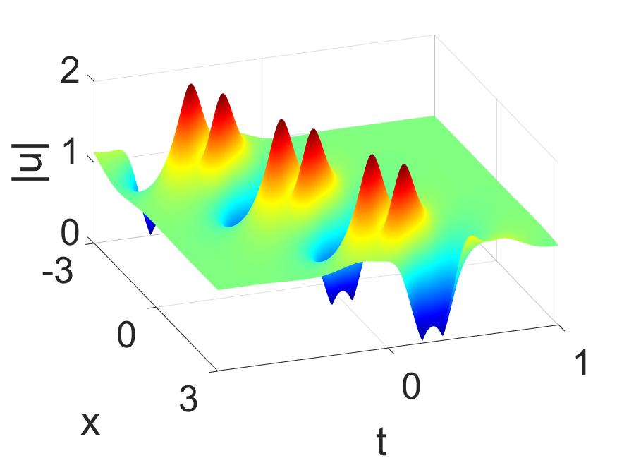
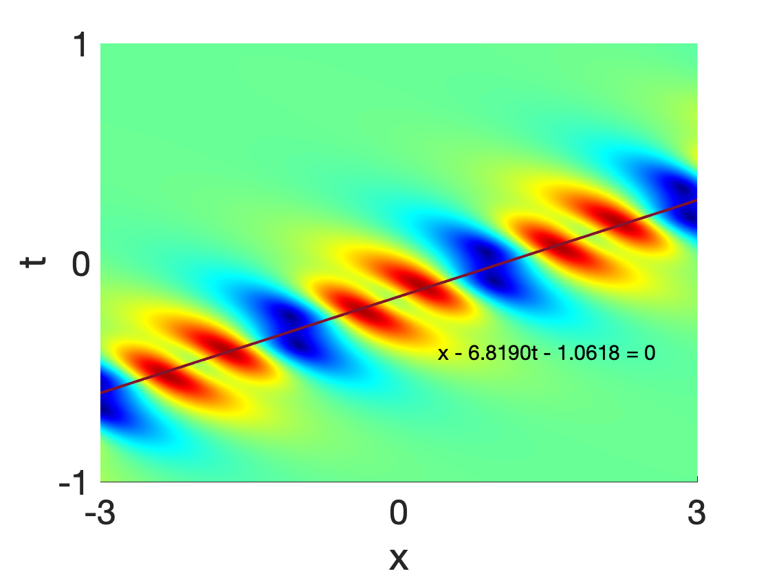
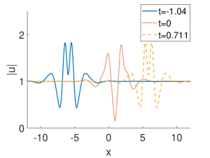
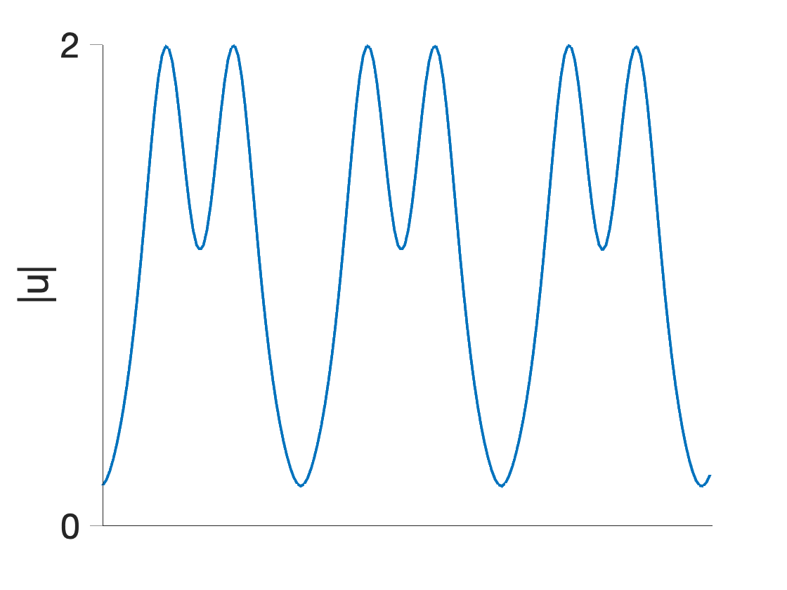
Figure 1: (Color online) A first-order breather solution with parameter values $c=-1,\kappa=-1/2,\xi_{11,0}=\xi_{12,0}=0$, $p_{11}=1+2\mathbf{i}$, $p_{12}=4/29-9\mathbf{i}/58$. (b) is the corresponding density plot of (a), (c) corresponds to the time evolution of (a) and (d) is the intersection between the plane $x-6.819t-1.0618=0$ and the breather.

In contrast with many integrable equations, a remarkable feature displayed by the Sasa-Satsuma equation (5) is that it possesses double-hump one soliton solutions [30]. Interestingly, this property can also be discovered in the breather solutions. This type of breather solution for parameters

$$c=-1,\quad\kappa=-1/2,\quad p_{11}=1+2\mathbf{i},\quad p_{12}=\frac{4}{29}+\frac{9}{58}\mathbf{i},\quad\xi_{11,0}=0,\quad\xi_{12,0}=0$$

is depicted in Figure 1. It is clear that this first-order breather contains two local maxima and three local minima in each period, where one local minimum is much bigger than the other two and located between two local maxima while the other two local minima are located on the same side of the local maxima. To be more precise, this breather reaches its peaks at $(x,t)\approx(1.6100,0.0700),(2.2000,0.1850)$, and a trough at $(x,t)\approx(1.9150,0.1250)$. Numerical computations indicate that its period is approximately 2.00112 and the local minima between two local maxima are located on the line $L:x\approx 6.819t+1.0618$ (see Figure 1). As displayed in Figure 1, taking the intersection of the line, the breather produces a double-hump periodic wave. Therefore, this breather may serve as a counterpart of the double-hump one soliton of the Sasa-Satsuma equation.

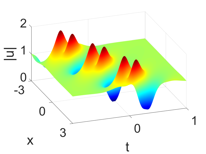
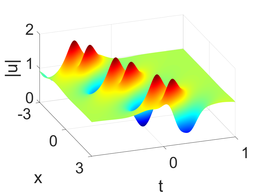
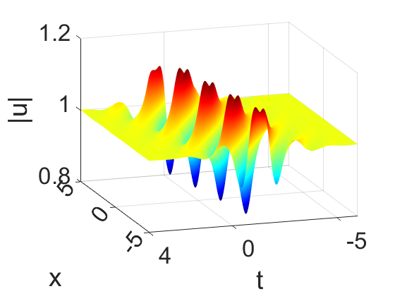
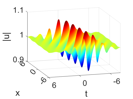
Figure 2: (Color online) First-order breather solutions with parameter values $c=-1,\kappa=-1/2,\xi_{11,0}=\xi_{12,0}=0$ and (a) $p_{11}=0.87+2\mathbf{i}$, (b) $p_{11}=0.8+2\mathbf{i}$, (c) $p_{11}=0.2+2\mathbf{i}$, (d) $p_{11}=0.1+2\mathbf{i}$, where $p_{12}$ is given by (54).

According to Remark Remark, the solutions (53) contain seven free real parameters. Varying these parameters will excite various interesting wave profiles of the breather solutions. To illustrate this, we fix the parameter values

$$c=-1,\quad\kappa=-1/2,\quad\Im{p_{11}}=2,\quad\xi_{11,0}=0,\quad\xi_{12,0}=0$$

and let $p=\Re{p_{11}}$ be free. In addition, we choose (see Remark Remark)

$$p_{12}=\frac{4\kappa^{2}p_{i1}-\mathbf{i}\kappa\left(p_{i1}^{2}-3\kappa^{2}\right)}{\kappa^{2}+p_{i1}^{2}}.$$ (54)

Then the wave profiles of the breather solutions can exhibit an intriguing sequence of transitions by altering the values of $p$. Geometrically these wave profiles can be defined as $(m,n)$-type, where $m$ and $n$ represent the numbers of local maxima and minima in one period respectively. If we start from $p=1$, then previous discussions imply that it corresponds to a $(2,3)$-type breather (see Figure 1). Subsequently, the two smaller local minima will approach each other and merge into a single minimum by changing $p$ and hence the wave profile becomes $(2,2)$-type (see Figures 2 and 2). On further changing $p$, the local minimum located between two local maxima is converted to a saddle point and the breather turns into $(2,1)$-type (see Figure 2). This is followed by $(1,1)$-type breather (see Figure 2) with the decrease of $p$ after two local maxima coalesce into a single maximum.

In the above process, the sign of $p$ is positive. Interestingly, similar behaviours can be observed as well for negative $p$. In this case, the wave profiles will traverse the three types of $(1,2),(2,2)$ and $(3,2)$ by varying $p$ (see Figure 3).

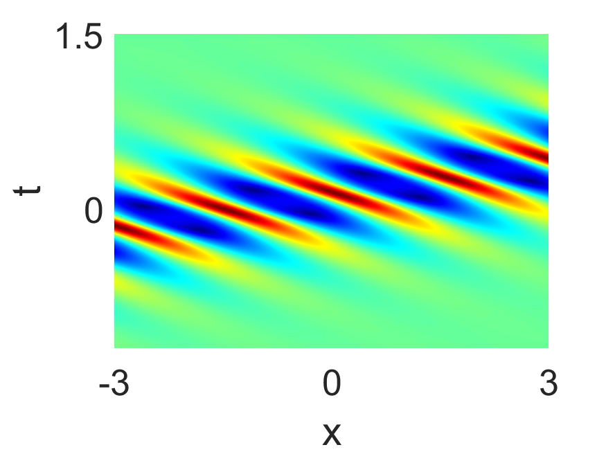
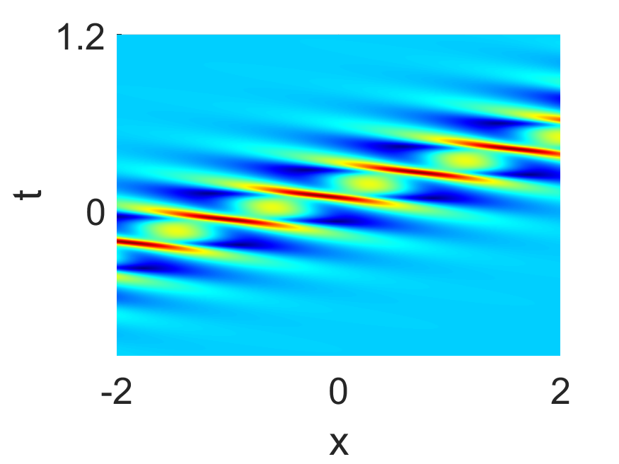
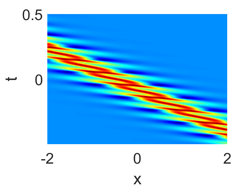
Figure 3: (Color online) First-order breather solutions with parameter values $c=-1,\kappa=-1/2,\xi_{11,0}=\xi_{12,0}=0$ and (a) $p_{11}=-0.6+2\mathbf{i}$, (b) $p_{11}=-1.6+2\mathbf{i}$, (c) $p_{11}=-3.5+2\mathbf{i}$, where $p_{12}$ is given by (54).

Note that when we fix the parameter values of $c,\kappa$ and $p_{11}$, the equation (8) yields two choices for $p_{12}$. Thus, distinct configurations of breather profiles for the same input parameters are possible. The first possible configuration is depicted in Figure 1, while the second complex root of the equation (8) gives $p_{12}=4/13-25/26\mathbf{i}$, leading to a completely different wave profile (see Figure 4).

4.2 Higher-order breather solutions

Second-order breather solutions to the equation (5) correspond to $N=2$ in (7). In this circumstance, the functions $\tau_{k}\,(k=0,1)$ could be obtained from (7) as

$$\tau_{0}=\left|\begin{array}[]{cccc}m_{11}^{(0)}&m_{12}^{(0)}&m_{13}^{(0)}&m_{14}^{(0)}\\ m_{21}^{(0)}&m_{22}^{(0)}&m_{23}^{(0)}&m_{24}^{(0)}\\ m_{31}^{(0)}&m_{32}^{(0)}&m_{33}^{(0)}&m_{34}^{(0)}\\ m_{41}^{(0)}&m_{42}^{(0)}&m_{43}^{(0)}&m_{44}^{(0)}\end{array}\right|,\quad\tau_{1}=\left|\begin{array}[]{cccc}m_{11}^{(1)}&m_{12}^{(1)}&m_{13}^{(1)}&m_{14}^{(1)}\\ m_{21}^{(1)}&m_{22}^{(1)}&m_{23}^{(1)}&m_{24}^{(1)}\\ m_{31}^{(1)}&m_{32}^{(1)}&m_{33}^{(1)}&m_{34}^{(1)}\\ m_{41}^{(1)}&m_{42}^{(1)}&m_{43}^{(1)}&m_{44}^{(1)}\end{array}\right|,$$

with matrix entries

$$m_{ij}^{(k)}=\sum\limits_{m,n=1}^{2}\frac{1}{p_{im}+p_{jn}}\left(\dfrac{a-p_{1m}}{a+p_{1n}}\right)^{k}e^{\xi_{im}+\xi_{jn}},\quad i,j=1,\dots,4,$$

where $a=\mathbf{i}\kappa$ is purely imaginary, $\xi_{im}=p_{im}x+p_{im}^{3}t+\xi_{im,0}\,(m=1,2)$, and the complex parameters $\xi_{im,0},p_{im}$ satisfy the relations (8) and (9). Similar to the first-order breather solutions, the second-order breather solutions can also be expressed in terms of trigonometric functions and hyperbolic functions. Since the expressions are very complicated, we omit their explicit forms.

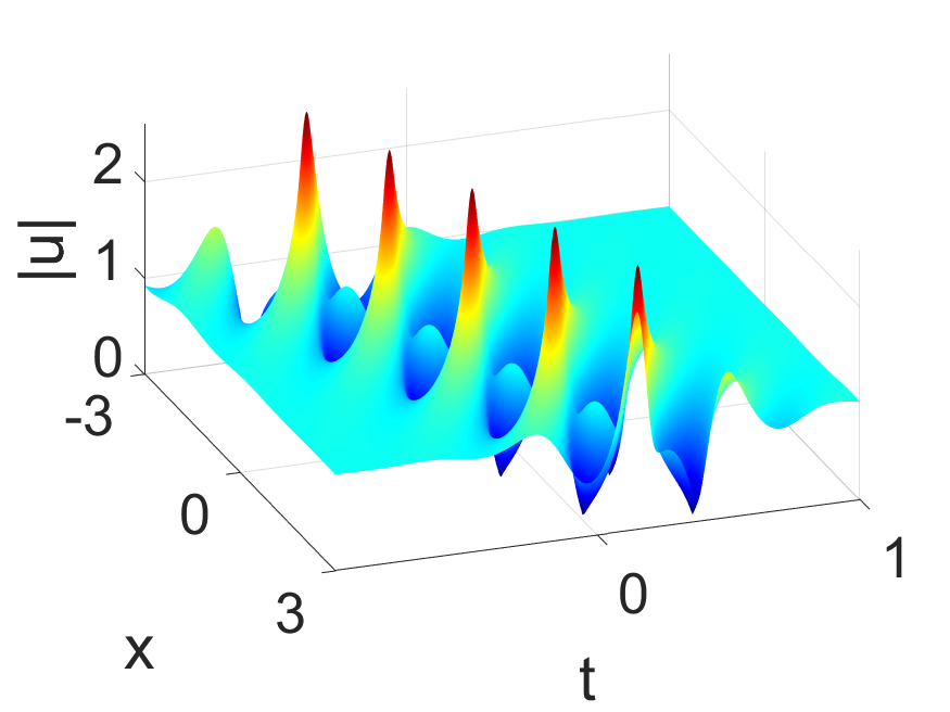
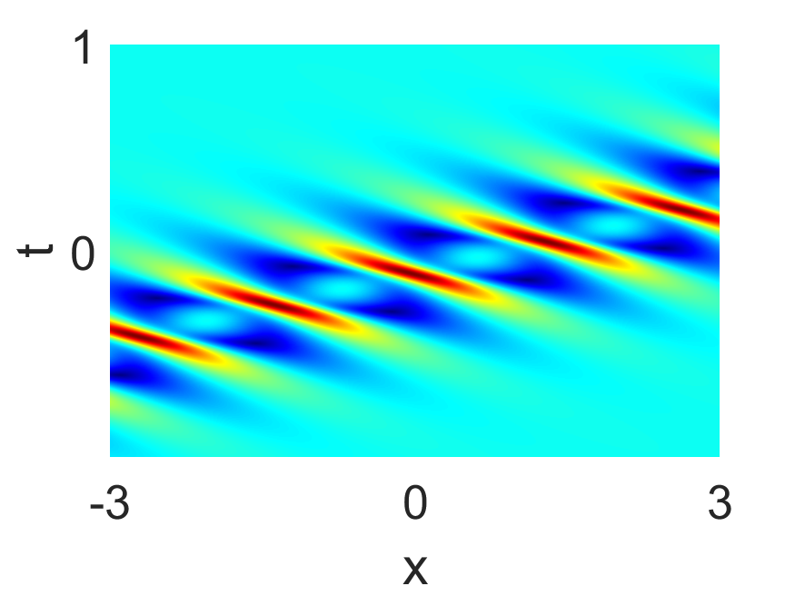
Figure 4: (Color online) First-order breather solutions with parameter values $c=-1,\kappa=-1/2,\xi_{11,0}=\xi_{12,0}=0$ and (a) $p_{11}=1+2\mathbf{i},p_{12}=4/13-25/26\mathbf{i}$. (b) is the corresponding density plots of (a).

As pointed in Remark Remark, second-order breather solutions contain the free parameters $\kappa,p_{i1}$ and $\xi_{im,0}\,(i,m=1,2)$, where $\kappa$ is real and $p_{i1},\xi_{im,0}$ are complex. A variety of fascinating wave profiles can be depicted for different choices of parameter values. Since second-order breathers describe the interactions between two first-order breathers, each of them can be classified into $(m_{1},n_{1})$-$(m_{2},n_{2})$-type if it comprises two first-order breathers that are $(m_{1},n_{1})$-type and $(m_{2},n_{2})$-type respectively. In Section 44.1, six types of first-order breathers have been illustrated, and hence they give rise to 21 types of second-order breathers. To demonstrate this, we take the parameters

$$c=-1,\quad\kappa=-1/2,\quad p_{11}=0.95+1.65\mathbf{i},\quad p_{12}=0.8+2\mathbf{i},\quad p_{21}=\frac{38}{221}+\frac{49}{442}\mathbf{i},$$

$$p_{22}=\dfrac{80}{689}+\dfrac{189}{1378}\mathbf{i},\quad\xi_{11,0}=0,\quad\xi_{12,0}=0,\quad\xi_{21,0}=0,\quad\xi_{22,0}=0.$$

As shown in Figure 5, this corresponds to a $(2,2)$-$(2,3)$-type second-order breather. It can also be seen clearly that the two breathers pass through each other without any change of shape or velocity, and thus the collision between them is elastic. If we choose other parameter values, then we may obtain second-order breathers consisting of two first-order breathers that belong to distinct types (see Figure 6) or the same type (see Figure 7).

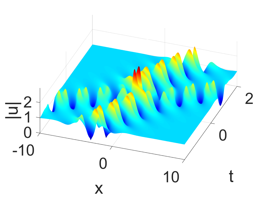
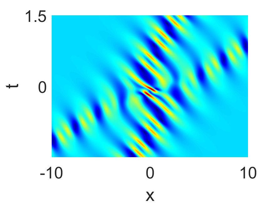
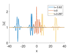
Figure 5: (Color online) Second-order breather solutions with parameter values $c=-1,\kappa=-1/2,p_{11}=0.95+1.65\mathbf{i},p_{21}=0.8+2\mathbf{i},\xi_{11,0}=\xi_{12,0}=0$, where $p_{12}$ and $p_{22}$ are given by (54). (b) is the corresponding density plot of (a), and (c) corresponds to the time evolution of (a).

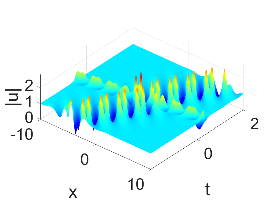
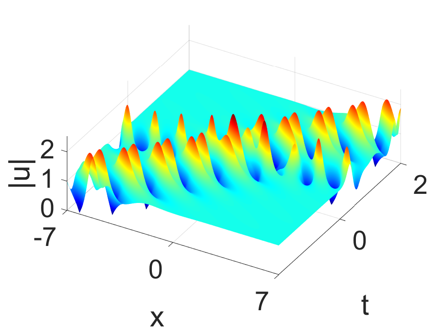
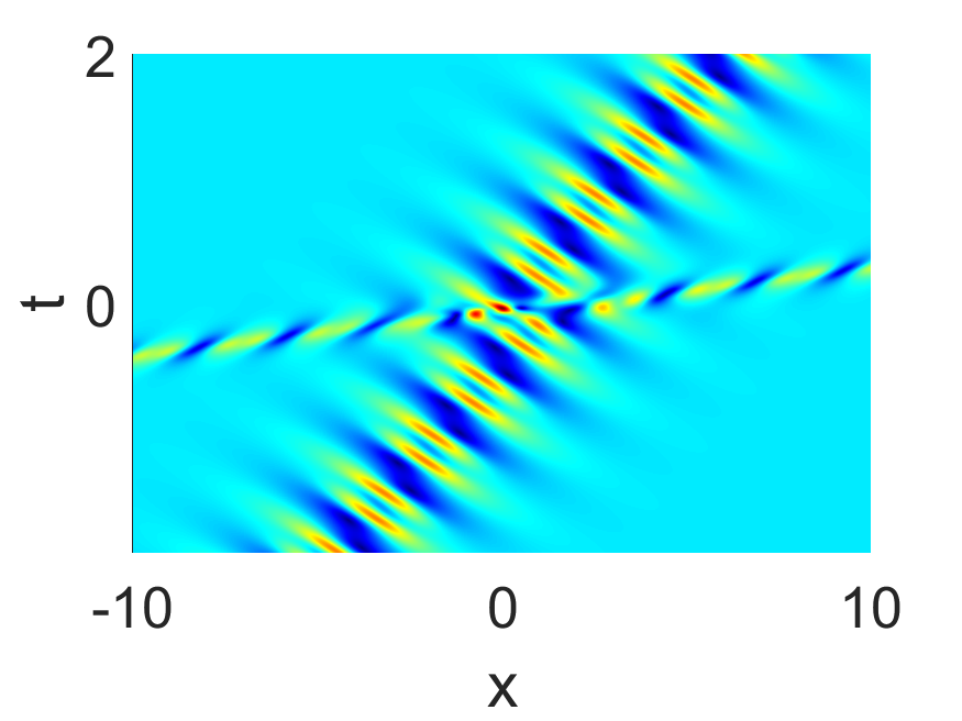
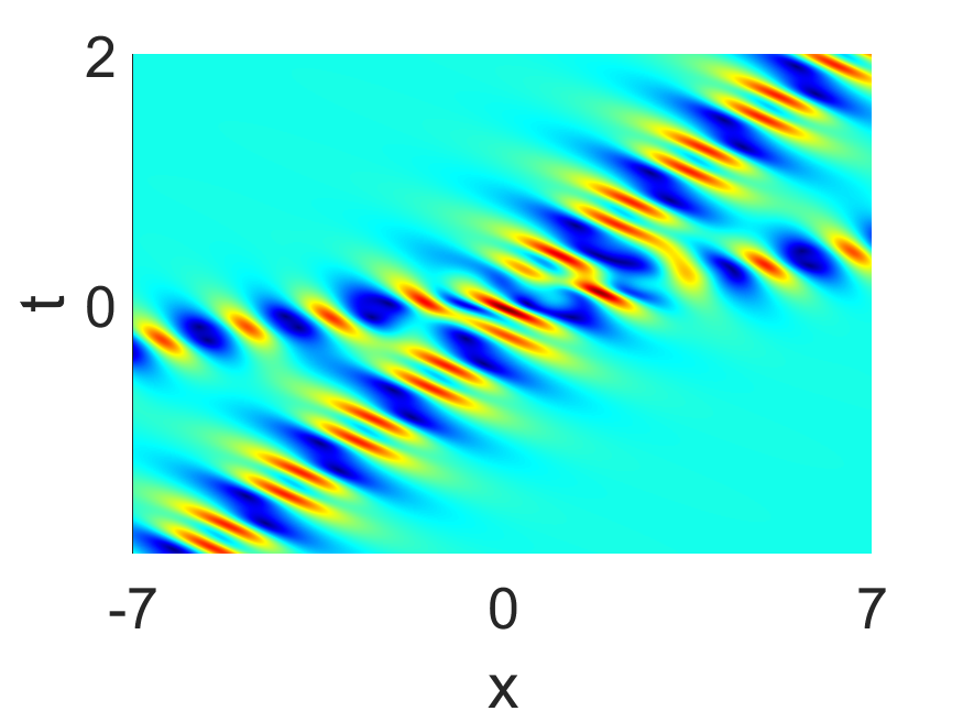
Figure 6: (Color online) Second-order breather solutions with parameter values $c=-1,\kappa=-1/2,\xi_{11,0}=\xi_{12,0}=0$ and (a) $p_{11}=0.8+3.2\mathbf{i}$, $p_{21}=0.95+1.65\mathbf{i}$, (b) $p_{11}=1+1.7\mathbf{i}$, $p_{21}=-0.65+2.5\mathbf{i}$, where $p_{12}$ and $p_{22}$ are given by (54). (c) and (d) are the corresponding density plots of (a) and (b), respectively.

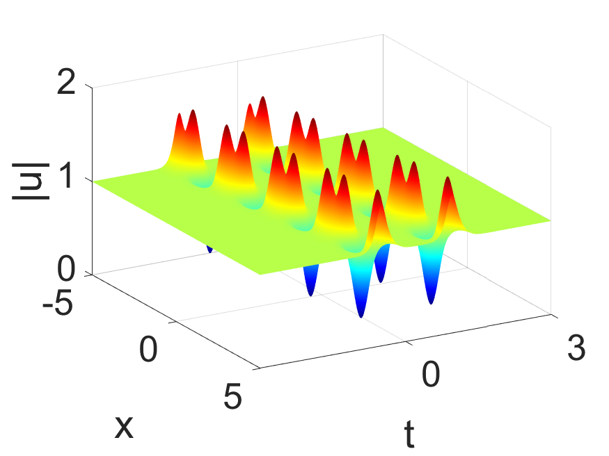
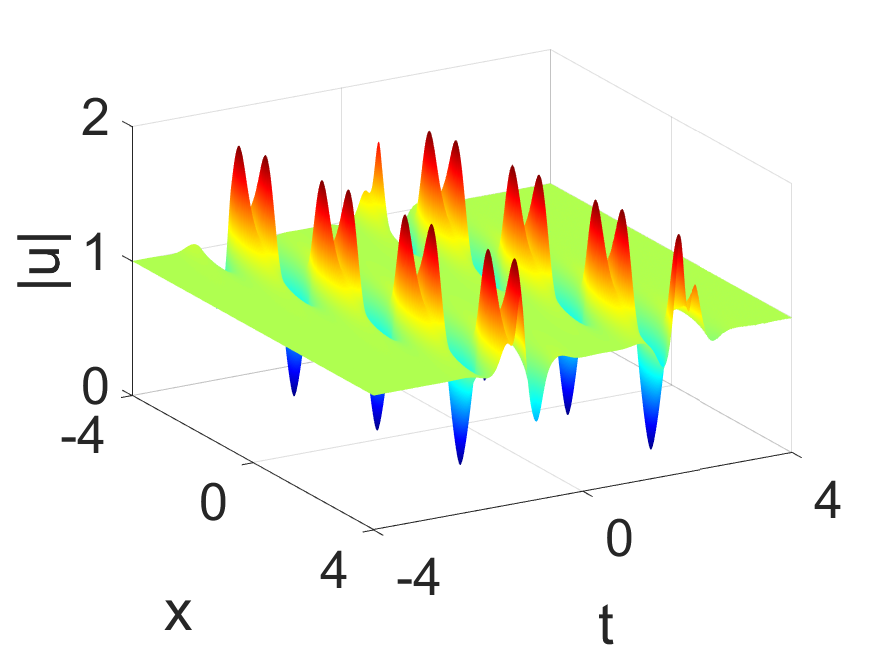
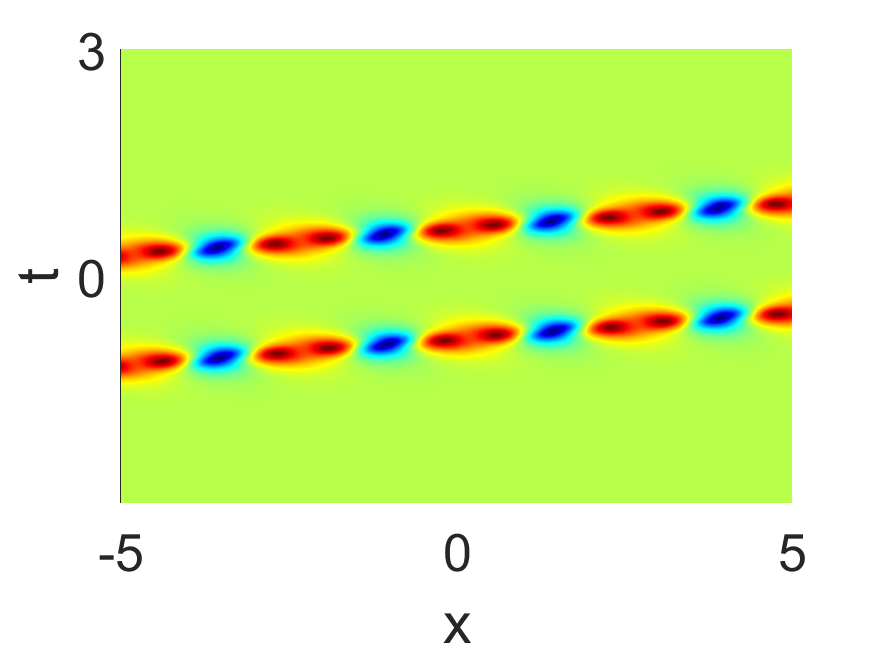
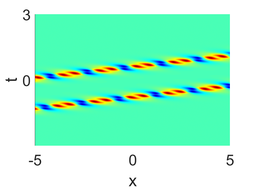
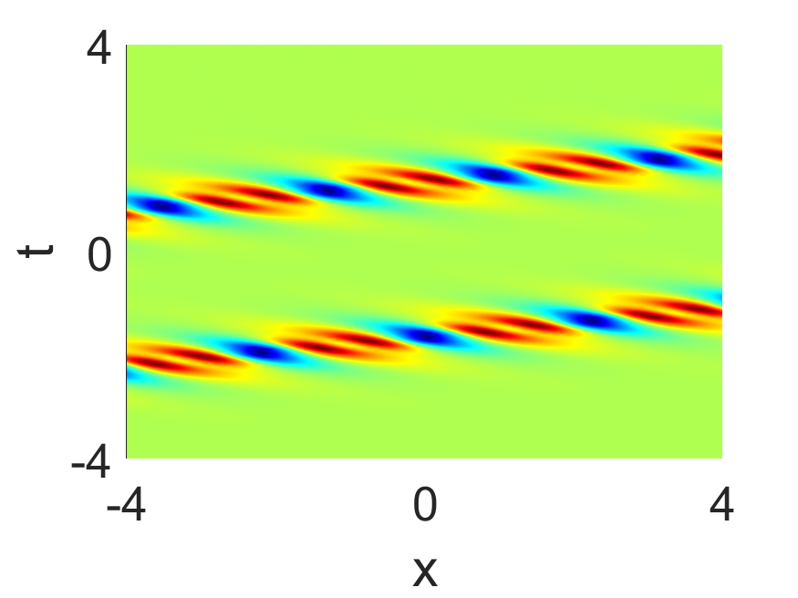
Figure 7: (Color online) Second-order breather solutions with parameter values $c=-1,\kappa=-1/2,\xi_{11,0}=1,\xi_{12,0}=0,\xi_{21,0}=\xi_{22,0}=0$ and (a) $p_{11}=0.8+2.5\mathbf{i}$, $p_{21}=0.8001+2.5\mathbf{i}$, (b) $p_{11}=1.3+2.3\mathbf{i}$, $p_{21}=1.3001+2.3\mathbf{i}$, (c) $p_{11}=0.8+2\mathbf{i}$, $p_{21}=0.8001+2\mathbf{i}$, where $p_{12}$ and $p_{22}$ are given by (54). (d), (e) and (f) are the corresponding density plots of (a), (b) and (c), respectively.

Finally, we can obtain $N$th-order breather solutions to the equation (5) from (7) by taking $N\geq 3$. In general, such solutions describe the superposition of $N$ first-order breathers. However, their explicit expressions are more complicated, so they will not be provided here. Instead, we only focus on the dynamical structures of third-order breather solutions ($N=3$), which consists of three first-order breathers. On the one hand, it is obvious that there are many more types of third-order breathers than second-order ones. On the other hand, third-order breathers exhibit more diverse collisions. As illustrated in Figure (8), the three first-order breathers may interact with each other in pairs or collide simultaneously.

5 Conclusion

In summary, we have derived general breather solutions to the SSE via the KP hierarchy reduction method. These solutions are expressed in terms of Gram-type determinants through transforming a set of bilinear equations in the KP hierarchy into the bilinear forms of the SSE. Owing to the complexity of the SSE and multiple corresponding bilinear equations in the KP hierarchy, the intermediate computations are much more involved compared with most of the integrable equations that can be solved by the same method. Furthermore, in addition to the common obstructions that appear in the KP hierarchy reduction method, i.e., the dimension reduction and the complex conjugate reduction, another obstacle that we have dealt with is the symmetry reduction.

The dynamics of breathers have been investigated. For first-order breathers, six types were found totally and some of them were shown to possess a double-hump structure. Interestingly, transitions among these first-order breathers can be achieved by changing the value of just one free real parameter in the solutions. In addition, various configurations of second- and third-order breathers have been illustrated. In particular, elastic collisions of second-order breathers were observed.

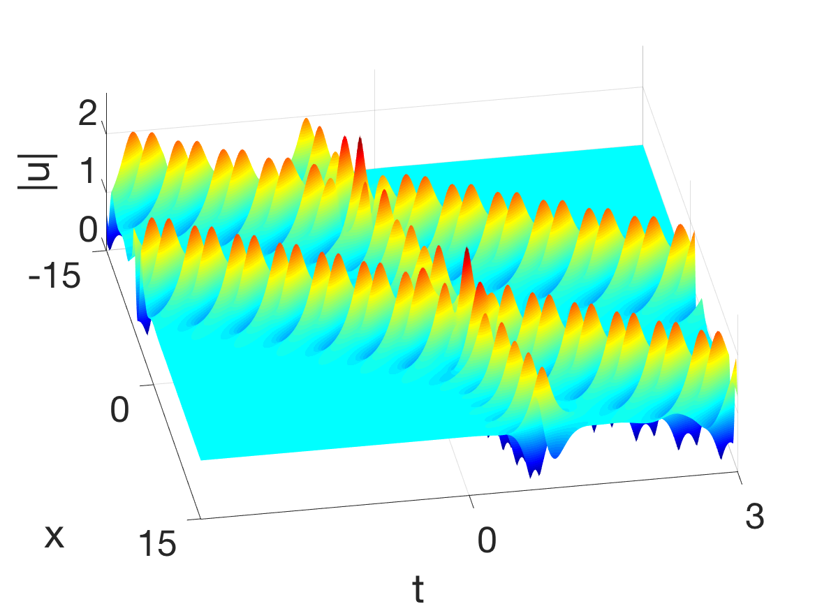
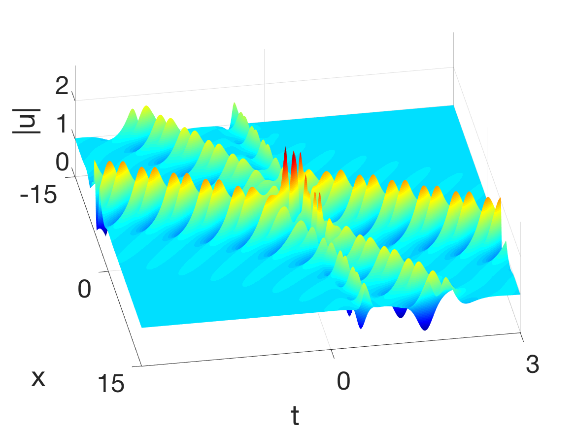
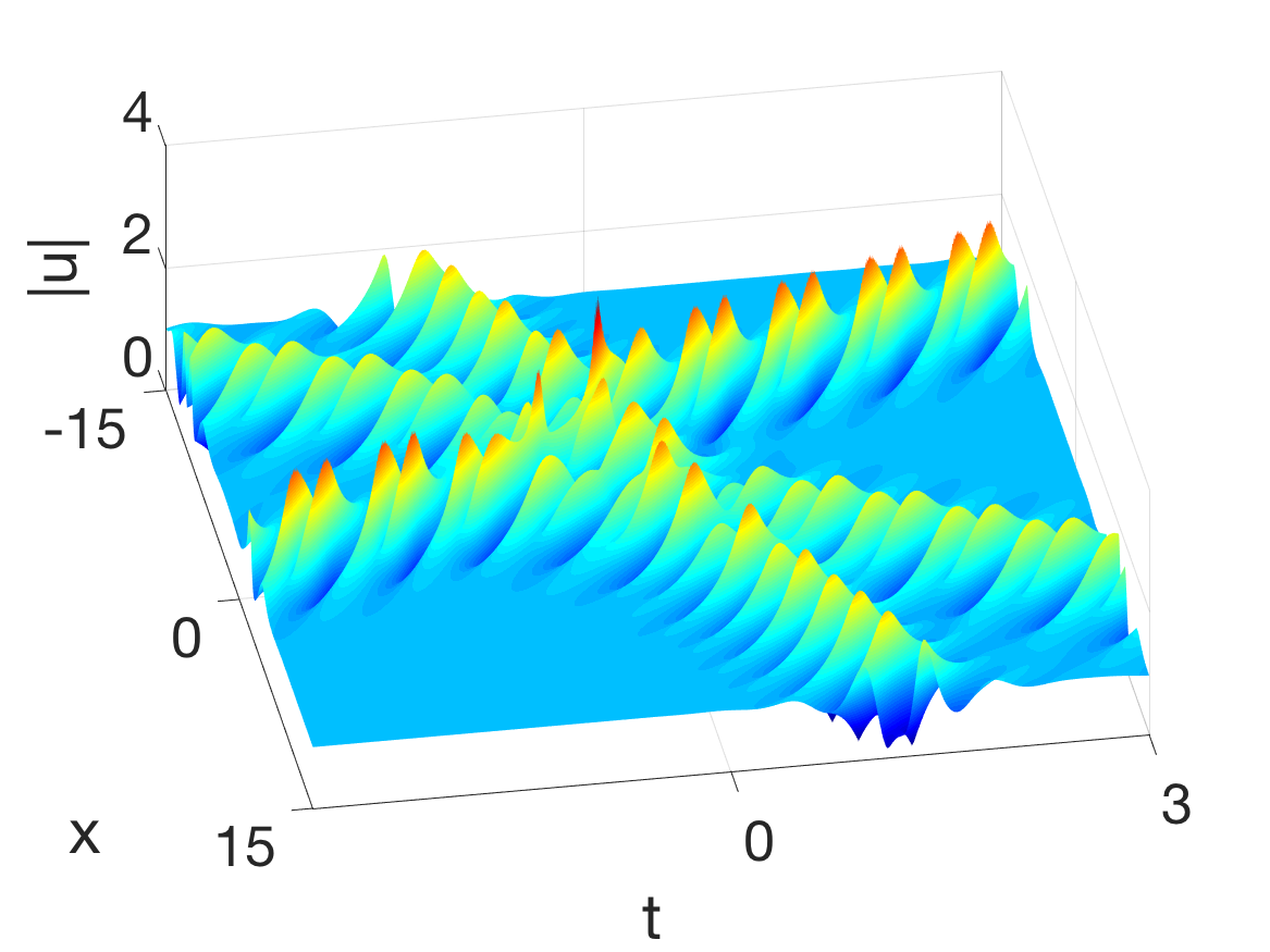
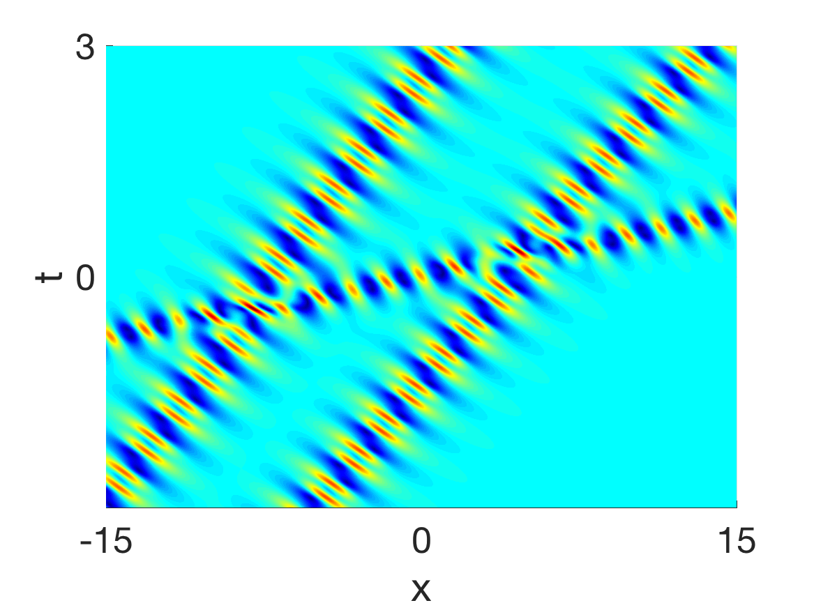
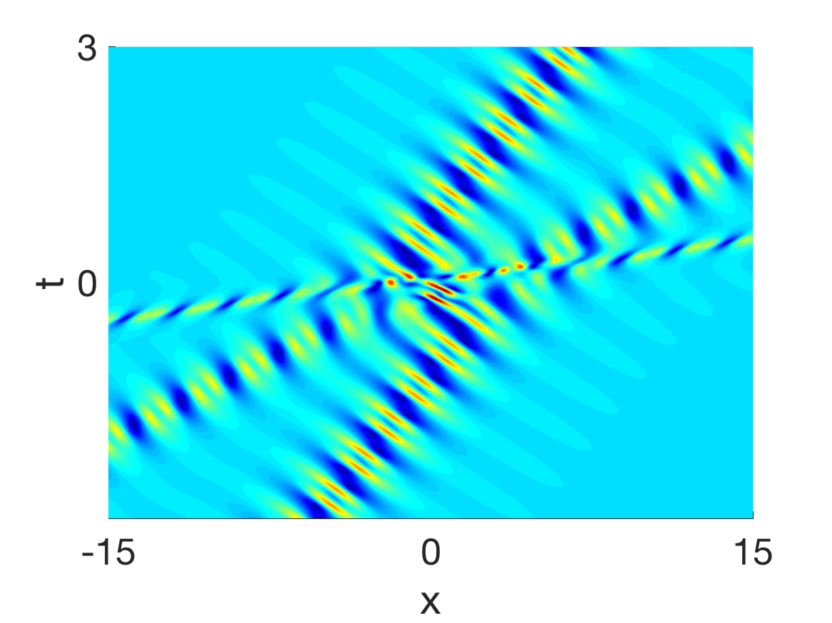
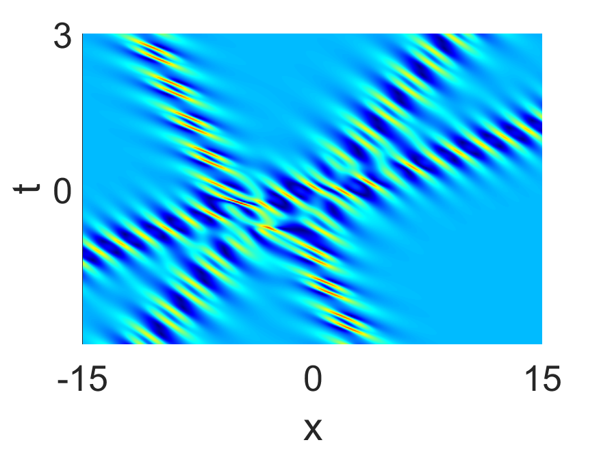
Figure 8: (Color online) Third-order breather solutions with parameter values $c=-1,\kappa=-1/2,\xi_{11,0}=\xi_{12,0}=0,\xi_{21,0}=\xi_{22,0}=0,\xi_{32,0}=0$ and (a) $p_{11}=1+1.7\mathbf{i}$, $p_{21}=-0.65+2.5\mathbf{i}$, $p_{31}=0.95+1.65\mathbf{i},$ $\xi_{31,0}=2$, (b) $p_{11}=0.95+1.65\mathbf{i}$, $p_{21}=0.8+2\mathbf{i}$, $p_{31}=0.8+3.2\mathbf{i},$ $\xi_{31,0}=2$, (c) $p_{11}=0.8+1.6\mathbf{i}$, $p_{21}=-0.65+2\mathbf{i}$, $p_{31}=1.3+1.3\mathbf{i},$ $\xi_{31,0}=4$, where $p_{12}$, $p_{22}$ and $p_{32}$ are given by (54). (d), (e) and (f) are the corresponding density plots of (a), (b) and (c), respectively.

Appendix

In this appendix, we show that the first-order breather solutions presented in Theorem 2.1 can be expressed in terms of trigonometric functions and hyperbolic functions. Let $N=1$, then Theorem 2.1 yields that

$$\tau_{0} = \left|\begin{array}[]{cc}\sum\limits_{m=1}^{2}\sum\limits_{n=1}^{2}\frac{1}{p_{1m}+p_{1n}}e^{\xi_{1m}+\xi_{1n}}&\sum\limits_{m=1}^{2}\sum\limits_{n=1}^{2}\frac{1}{p_{1m}+p_{1n}^{*}}e^{\xi_{1m}+\xi_{1n}^{*}}\\ \sum\limits_{m=1}^{2}\sum\limits_{n=1}^{2}\frac{1}{p_{1m}^{*}+p_{1n}}e^{\xi_{1m}^{*}+\xi_{1n}}&\sum\limits_{m=1}^{2}\sum\limits_{n=1}^{2}\frac{1}{p_{1m}^{*}+p_{1n}^{*}}e^{\xi_{1m}^{*}+\xi_{1n}^{*}}\\ \end{array}\right|$$ (58)

$$= |m_{1}|^{2}-m_{2}^{2},$$ (59)

where

$$m_{1}=\sum\limits_{m=1}^{2}\sum\limits_{n=1}^{2}\frac{1}{p_{1m}+p_{1n}}e^{\xi_{1m}+\xi_{1n}},\quad m_{2}=\sum\limits_{m=1}^{2}\sum\limits_{n=1}^{2}\frac{1}{p_{1m}+p_{1n}^{*}}e^{\xi_{1m}+\xi_{1n}^{*}}.$$

Denote by $p_{11}=A+\mathbf{i}B,p_{12}=R+\mathbf{i}S,\xi_{11,0}=\alpha_{1}+\mathbf{i}\beta_{1},\xi_{12,0}=\alpha_{2}+\mathbf{i}\beta_{2}$, where $p_{11}$ and $p_{12}$ satisfy (8), then we have

$$\xi_{11}=X+\mathbf{i}Y=Ax+(A^{3}-3AB^{2})t+\alpha_{1}+\mathbf{i}\left[Bx+\left(3A^{2}B-B^{3}\right)t+\beta_{1}\right],$$

$$\xi_{12}=W+\mathbf{i}V=Rx+(R^{3}-3RS^{2})t+\alpha_{2}+\mathbf{i}\left[Sx+\left(3R^{2}S-S^{3}\right)t+\beta_{2}\right].$$

After some tedious algebra, we can rewrite $\tau_{0}$ in the form

$$\tau_{0} = e^{2W+2X}\left\{c_{0}+M_{1}\cosh(2W-2X-\theta_{1})\right.$$ (60)

$$+(c_{1}+c_{2})\cos(V-Y)\cosh(W-X)+(c_{1}-c_{2})\cos(V-Y)\sinh(W-X)$$

$$+(d_{1}+d_{2})\sin(V-Y)\cosh(W-X)+(d_{1}-d_{2})\sin(V-Y)\sinh(W-X)$$

$$\left.+(c_{3}+d_{3})^{1/2}\cos(2V-2Y-\theta_{2})\right\}$$

where

$c_{1}=\dfrac{2(R(A+R)+S(B+S))}{\left(R^{2}+S^{2}\right)K}-\dfrac{2(A+R)}{RL}$,	$d_{1}=\dfrac{2(AS-BR)}{\left(R^{2}+S^{2}\right)K}-\dfrac{2(S-B)}{RL}$,
$c_{2}=\dfrac{2(A(A+R)+B(B+S))}{\left(A^{2}+B^{2}\right)K}-\dfrac{2(A+R)}{AL}$,	$d_{2}=\dfrac{2(AS-BR)}{\left(A^{2}+B^{2}\right)K}-\dfrac{2(S-B)}{AL}$,
$c_{3}=\dfrac{AR+BS}{2\left(A^{2}+B^{2}\right)\left(R^{2}+S^{2}\right)}-\dfrac{2(A+R)^{2}-2(B-S)^{2}}{L^{2}}$,
$d_{3}=\dfrac{AS-BR}{2\left(A^{2}+B^{2}\right)\left(R^{2}+S^{2}\right)}+\dfrac{4(A+R)(B-S)}{L^{2}}$,
$c_{0}=\dfrac{4}{K}-\dfrac{2}{L}-\dfrac{1}{2AR}$, $\qquad K=(A+R)^{2}+(B+S)^{2}$,	$L=(A+R)^{2}+(B-S)^{2}$,
$M_{1}=2\sqrt{\sigma_{1}\sigma_{2}}$, $\qquad\theta_{1}=\ln(\sigma_{2}/\sigma_{1})/2$, $\qquad\theta_{2}=\arctan(d_{3}/c_{3})$,
$\sigma_{1}=\dfrac{S^{2}}{4R^{2}\left(R^{2}+S^{2}\right)}$, $\qquad\sigma_{2}=\dfrac{B^{2}}{4A^{2}\left(A^{2}+B^{2}\right)}$.

Similarly, we have

$$\tau_{1} = e^{2W+2X}\left\{e_{0}+M_{2}\cosh(2W-2X-\theta_{3})\right.$$ (61)

$$+(e_{1}+e_{2})\cos(V-Y)\cosh(W-X)+(e_{1}-e_{2})\cos(V-Y)\sinh(W-X)$$

$$+(f_{1}+f_{2})\sin(V-Y)\cosh(W-X)+(f_{1}-f_{2})\sin(V-Y)\sinh(W-X)$$

$$+(e_{3}+f_{3})^{1/2}\cos(2V-2Y-\theta_{4})$$

$$+i\left[\hat{e}_{0}+\hat{M}_{2}\cosh(2W-2X-\hat{\theta}_{3})\right.$$

$$+(\hat{e}_{1}+\hat{e}_{2})\cos(V-Y)\cosh(W-X)+(\hat{e}_{1}-\hat{e}_{2})\cos(V-Y)\sinh(W-X)$$

$$+(\hat{f}_{1}+\hat{f}_{2})\sin(V-Y)\cosh(W-X)+(\hat{f}_{1}-\hat{f}_{2})\sin(V-Y)\sinh(W-X)$$

$$\left.\left.+(\hat{e}_{3}+\hat{f}_{3})^{1/2}\cos(2V-2Y-\hat{\theta}_{4})\right]\right\},$$

where

$$e_{0} = \Re(K_{22}+K_{23}+K_{32}+K_{33}-L_{14}-L_{22}-L_{33}-L_{41}),$$

$$e_{1} = \Re(K_{24}+K_{34}+K_{42}+K_{43}-L_{24}-L_{43}-L_{42}-L_{34}),$$

$$f_{1} = \Im(-K_{24}-K_{34}+K_{42}+K_{43}+L_{24}+L_{43}-L_{42}-L_{34}),$$

$$e_{2} = \Re(K_{12}+K_{13}+K_{21}+K_{31}-L_{13}-L_{21}-L_{31}-L_{12}),$$

$$f_{2} = \Im(-K_{12}-K_{13}+K_{21}+K_{31}+L_{13}+L_{21}-L_{31}-L_{12}),$$

$$e_{3} = \Re(K_{14}+K_{41}-L_{23}-L_{32}),$$

$$f_{3} = \Im(-K_{14}+K_{41}-L_{23}+L_{32}),$$

$$\hat{e}_{0} = \Im(K_{22}+K_{23}+K_{32}+K_{33}-L_{14}-L_{22}-L_{33}-L_{41}),$$

$$\hat{e}_{1} = \Im(K_{24}+K_{34}+K_{42}+K_{43}-L_{24}-L_{43}-L_{42}-L_{34}),$$

$$\hat{f}_{1} = \Re(K_{24}+K_{34}-K_{42}-K_{43}-L_{24}-L_{43}+L_{42}+L_{34}),$$

$$\hat{e}_{2} = \Im(K_{12}+K_{13}+K_{21}+K_{31}-L_{13}-L_{21}-L_{31}-L_{12}),$$

$$\hat{f}_{2} = \Re(K_{12}+K_{13}-K_{21}-K_{31}-L_{13}-L_{21}+L_{31}+L_{12}),$$

$$\hat{e}_{3} = \Im(K_{14}+K_{41}-L_{23}-L_{32}),$$

$$\hat{f}_{3} = \Re(K_{14}-K_{41}+L_{23}-L_{32}),$$

$$M_{2} = 2\sqrt{\Re((K_{11}-L_{11})(K_{44}-L_{44}))},\quad\hat{M}_{2}=2\sqrt{\Im((K_{11}-L_{11})(K_{44}-L_{44}))},$$

$$\theta_{3} = \ln\Re((K_{11}-L_{11})/(K_{44}-L_{44}))/2,\quad\hat{\theta}_{3}=\ln\Im((K_{11}-L_{11})/(K_{44}-L_{44}))/2,$$

$$\theta_{4} = \arctan(f_{3}/e_{3}),\quad\hat{\theta}_{4}=\arctan(\hat{f}_{3}/\hat{e}_{3}),$$

and $K_{kl},L_{kl},(k,l=1,2,3,4)$ are given by

$$K_{kl}=n^{(k)}_{11}\times n^{(l)}_{22},\quad L_{kl}=n^{(k)}_{12}\times n^{(l)}_{21},$$ (62)

with $(i,j=1,2)$

$$n^{(1)}_{ij}=\frac{(\mathbf{i}\kappa-p_{i,1})}{(p_{j,1}+a)(p_{i,1}+p_{j,1})},\quad n^{(2)}_{ij}=\frac{(\mathbf{i}\kappa-p_{i,1})}{(p_{j,2}+a)(p_{i,1}+p_{j,2})},$$ (63)

$$n^{(3)}_{ij}=\frac{(\mathbf{i}\kappa-p_{i,2})}{(p_{j,1}+a)(p_{i,2}+p_{j,1})},\quad n^{(4)}_{ij}=\frac{(\mathbf{i}\kappa-p_{i,2})}{(p_{j,2}+a)(p_{i,2}+p_{j,2})}.$$ (64)

As a consequence, the first-order breather solutions of the Sasa-Satsuma equation (5) can be rewritten as

$$u=\frac{\tau_{1}(x-6ct,t)}{\tau_{0}(x-6ct,t)}e^{\mathrm{i}\left(\kappa(x-6ct)-\kappa^{3}t\right)},$$

where $\tau_{0}$ and $\tau_{1}$ are given by (60) and (61) respectively.

References

- [1] Ablowitz M, Kaup D, Newell A, Segur H. 1973 Method for solving the sine-Gordon equation. Phys. Rev. Lett. 30, 1262–1264. (doi:10.1103/PhysRevLett.30.1262)
- [2] Akhmediev N, Eleonskii V, Kulagin N. 1987 First-order exact solutions of the nonlinear Schrödinger equation. Theor. Math. Phys. 72, 809–818. (doi:10.1007/BF01017105)
- [3] Akhmediev N, Ankiewicz A. 1997 Solitons, Non-linear Pulses and Beams. London: Chapman & Hall.
- [4] Sievers A, Takeno S. 1988 Intrinsic localized modes in anharmonic crystals. Phys. Rev. Lett. 61, 970. (doi:10.1103/PhysRevLett.61.970)
- [5] Page J. 1990 Asymptotic solutions for localized vibrational modes in strongly anharmonic periodic systems. Phys. Rev. B 41, 7835. (doi:10.1103/PhysRevB.41.7835)
- [6] Eisenberg H, Silberberg Y, Morandotti R, Boyd A, Aitchison J. 1998 Discrete spatial optical solitons in waveguide arrays. Phys. Rev. Lett. 81, 3383. (doi:10.1103/PhysRevLett.81.3383)
- [7] Sukorukov A, Kivshar Y, Eisenberg H, Silberberg Y. 2003 Spatial optical solitons in waveguide arrays. IEEE J. Quantum Electron. 39, 31–50. (doi:10.1109/JQE.2002.806184)
- [8] Trias E, Mazo J, Orlando T. 2000 Discrete breathers in nonlinear lattices: Experimental detection in a Josephson array. Phys. Rev. Lett. 84, 741. (doi:10.1103/PhysRevLett.84.741)
- [9] Binder P, Abraimov D, Ustinov A, Flach S, Zolotaryuk Y. 2000 Observation of breathers in Josephson ladders Phys. Rev. Lett. 84, 745. (doi:10.1103/PhysRevLett.84.745)
- [10] Schwarz U, English L, Sievers A. 1999 Experimental generation and observation of intrinsic localized spin wave modes in an antiferromagnet. Phys. Rev. Lett. 83, 223. (doi:10.1103/PhysRevLett.83.223)
- [11] Sato M, Hubbard B, Sievers A, Ilic B, Czaplewski D, Craighead H. 2003 Observation of locked intrinsic localized vibrational modes in a micromechanical oscillator array. Phys. Rev. Lett. 90, 044102. (doi:10.1103/PhysRevLett.90.044102)
- [12] Yuen H, Lake B. 1980 Instabilities of waves on deep water. Annu. Rev. Fluid Mech. 12, 303–334. (doi:10.1146/annurev.fl.12.010180.001511)
- [13] Zakharov V, Ostrovsky L. 2009 Modulation instability: the beginning. Phys. D. 238, 540–548. (doi:10.1016/j.physd.2008.12.002)
- [14] Dysthe K, Krogstad H, Müller P. 2008 Oceanic rogue waves. Annu. Rev. Fluid Mech. 40, 287–310. (doi:10.1146/annurev.fluid.40.111406.102203)
- [15] Feng B, Ling L, Zhu Z. 2021 A focusing and defocusing semi-discrete complex short-pulse equation and its various soliton solutions. Proc. R. Soc. A 477, 20200853. (doi:10.1098/rspa.2020.0853)
- [16] Chowdury A, Krolikowski W, Akhmediev N. 2017 Breather solutions of a fourth-order nonlinear Schrödinger equation in the degenerate, soliton, and rogue wave limits. Phys. Rev. E 96, 042209. (doi:10.1103/PhysRevE.96.042209)
- [17] Benney D, Newell A. 1967 The propagation of nonlinear wave envelopes. J. Math. Phys. 46, 133–139. (doi:10.1002/sapm1967461133)
- [18] Agrawal, G. 1995 Nonlinear fiber optics. New York, USA: Academic Press.
- [19] Zakharov V. 1972 Collapse of Langmuir waves. Sov. Phys. JETP 35, 908–914.
- [20] Dalfovo F, Giorgini S, Pitaevskii L, Stringari S. 1999 Theory of Bose-Einstein condensation in trapped gases. Rev. Mod. Phys. 71, 463. (doi:10.1103/RevModPhys.71.463)
- [21] Akhmediev N, Korneev V. 1986 Modulation instability and periodic solutions of the nonlinear Schrödinger equation. Theor. Math. Phys. 69, 1089–1093. (doi:10.1007/BF01037866)
- [22] Ohta Y, Yang J. 2013 General high-order rogue waves and their dynamics in the nonlinear Schrödinger equation. Proc. R. Soc. A 468, 1716–1740. (doi:10.1098/rspa.2011.0640)
- [23] Chen J, Pelinovsky DE. 2018 Rogue periodic waves of the focusing nonlinear Schrödinger equation. Proc. R. Soc. A 474, 20170814. (doi:10.1098/rspa.2017.0814)
- [24] Kuznetsov E. 1977 Solitons in a parametrically unstable plasma. Dokl. Akad. Nauk SSSR 236, 575–577.
- [25] Ma Y. 1979 The perturbed plane-wave solutions of the cubic Schrödinger equation. Stud. Appl. Math. 60, 43–58. (doi:10.1002/sapm197960143)
- [26] Peregrine D. 1983 Water waves, nonlinear Schrödinger equations and their solutions. J. Austral. Math. Soc. Ser. B 25, 16–43. (doi:10.1017/S0334270000003891)
- [27] Zhang G, Yan Z. 2018 The n-component nonlinear Schrödinger equations: dark–bright mixed N-and high-order solitons and breathers, and dynamics. Proc. R. Soc. A 474, 20170688. (doi:10.1098/rspa.2017.0688)
- [28] Agrawal G. 2011 Nonlinear fiber optics: its history and recent progress. J. Opt. Soc. Am. B 28, A1–A10. (doi:10.1364/JOSAB.28.0000A1)
- [29] Porsezian K, Daniel M, Lakshmanan M. 1992 On the integrability aspects of the one-dimensional classical continuum isotropic biquadratic Heisenberg spin chain. J. Math. Phys. 33, 1807–1816. (doi:10.1063/1.529658)
- [30] Sasa N, Satsuma J. 1991 New-type of soliton solutions for a higher-order nonlinear Schrödinger equation. J. Phys. Soc. Jpn. 60, 409–417. (doi:10.1143/JPSJ.60.409)
- [31] Xu J, Fan E. 2013 The unified transform method for the Sasa–Satsuma equation on the half-line. Proc. R. Soc. A 469, 20130068. (doi:10.1098/rspa.2013.0068)
- [32] Kundu A. 1984 Landau–Lifshitz and higher-order nonlinear systems gauge generated from nonlinear Schrödinger-type equations. J. Math. Phys. 25, 3433–3438. (doi:10.1063/1.526113)
- [33] Gedalin M, Scott T, Band Y. 1997 Optical solitary waves in the higher order nonlinear Schrödinger equation. Phys. Rev. Lett. 78, 448. (doi:10.1103/PhysRevLett.78.448)
- [34] Mihalache D, Torner L, Moldoveanu F, Panoiu N, Truta N. 1993 Inverse-scattering approach to femtosecond solitons in monomode optical fibers. Phys. Rev. E 48, 4699. (doi:10.1103/PhysRevE.48.4699)
- [35] Gilson C, Hietarinta J, Nimmo J, Ohta Y. 2003 Sasa-Satsuma higher-order nonlinear Schrödinger equation and its bilinearization and multisoliton solutions. Phys. Rev. E 68, 016614. (doi:10.1103/PhysRevE.68.016614)
- [36] Shi X, Li J, Wu C. 2019 Dynamics of soliton solutions of the nonlocal Kundu-nonlinear Schrödinger equation. Chaos 29, 023120. (doi:10.1063/1.5080921)
- [37] Mihalache D, Truta N, Crasovan L-C. 1997 Painlevé analysis and bright solitary waves of the higher-order nonlinear Schrödinger equation containing third-order dispersion and self-steepening term. Phys. Rev. E 56, 1064. (doi:10.1103/PhysRevE.56.1064)
- [38] Solli D, Ropers C, Koonath P, Jalali B. 2007 Optical rogue waves. Nature 450, 1054–1057. (doi:10.1038/nature06402)
- [39] Ohta Y. 2010 Dark soliton solution of Sasa-Satsuma equation. AIP Conf. Proc. 1212, 114–121. (doi:10.1063/1.3367022)
- [40] Chen S. 2013 Twisted rogue-wave pairs in the Sasa-Satsuma equation. Phys. Rev. E 88, 023202. (doi:10.1103/PhysRevE.88.023202)
- [41] Mu G, Qin Z. 2016 Dynamic patterns of high-order rogue waves for Sasa–Satsuma equation. Nonlinear Anal. Real World Appl. 31, 179–209. (doi:10.1016/j.nonrwa.2016.01.001)
- [42] Akhmediev N, Soto-Crespo J, Devine N, Hoffmann N. 2015 Rogue wave spectra of the Sasa–Satsuma equation. Phys. D 294, 37–42. (doi:10.1016/j.physd.2014.11.006)
- [43] Ling L. 2016 The algebraic representation for high order solution of Sasa-Satsuma equation. Discrete Contin. Dyn. Syst. Ser. S 9, 1975. (doi:10.3934/dcdss.2016081)
- [44] Liu H, Geng X, Xue B. 2018 The Deift–Zhou steepest descent method to long-time asymptotics for the Sasa–Satsuma equation. J. Differ. Equ. 265, 5984–6008. (doi:10.1016/j.jde.2018.07.026)
- [45] Chen J, Feng B, Maruno K-i, Ohta Y. 2018 The derivative Yajima-Oikawa system: bright, dark soliton and breather solutions. Stud. Appl. Math. 141, 145–185. (doi:10.1111/sapm.12216)
- [46] Feng B, Luo X, Ablowitz M, Musslimani Z. 2018 General soliton solution to a nonlocal nonlinear Schrödinger equation with zero and nonzero boundary conditions. Nonlinearity 31, 5385. (doi:10.1088/1361-6544/aae031)
- [47] Rao J, Porsezian K, He J, Kanna T. 2018 Dynamics of lumps and dark–dark solitons in the multi-component long-wave–short-wave resonance interaction system. Proc. R. Soc. A 474, 20170627. (doi:10.1098/rspa.2017.0627)
- [48] Chen J, Chen L, Feng B, Maruno K-i. 2019 High-order rogue waves of a long-wave–short-wave model of newell type. Phys. Rev. E 100, 052216. (doi:10.1103/PhysRevE.100.052216)
- [49] Li M, Fu H, Wu C. 2020 General soliton and (semi-) rational solutions to the nonlocal Mel’nikov equation on the periodic background. Stud. Appl. Math. 145, 97–136. (doi:10.1111/sapm.12313)
- [50] Hirota R. 2004 The Direct Method in Soliton Theory. Cambridge, UK: Cambridge University Press.
- [51] Jimbo M, Miwa T. 1983 Solitons and infinite dimensional Lie algebras. Publ. Res. Inst. Math. Sci. 19, 943–1001. (doi:10.2977/prims/1195182017)