Collaborative Graph Contrastive Learning: Data Augmentation Composition May Not be Necessary for Graph Representation Learning

Abstract.

Unsupervised graph representation learning is a non-trivial topic for graph data. The success of contrastive learning in the unsupervised representation learning of structured data inspires similar attempts on the graph. The current unsupervised graph representation learning and pre-training using the contrastive loss are mainly based on the contrast between handcrafted augmented graph data. However, the graph data augmentation is still not well-explored due to the uncontrollable invariance. In this paper, we propose a novel collaborative graph neural networks contrastive learning framework (CGCL), which uses multiple graph encoders to observe the graph. Features observed from different views act as the graph augmentation for contrastive learning between graph encoders, which avoid inducing any perturbation to guarantee the invariance. CGCL can handle both graph-level and node-level representation learning. Extensive experiments demonstrate the advantages of CGCL in unsupervised graph representation learning and the non-necessity of handcrafted data augmentation composition for graph representation learning. Our code are available at: Clickable link.

1. Introduction

Graphs have been proven to possess outstanding capabilities in representing diverse types of data from various research fields, including social networks (shi2016survey, ), financial risk control (ren2019ensemfdet, ), biological protein analysis (strokach2020fast, ), and intelligent transportation systems (zhou2020variational, ). The advantage of graph-structured data in terms of information representation is that it can not only contain the attribute information of individual units (i.e., nodes) but also explicitly provide the connection information (i.e., edges) between these units. Due to this ability, many applications exhibit the favorable property of graph-structured data, which makes learning effective graph representations for downstream tasks a non-trivial problem.

Recently, graph neural networks (GNNs) (velivckovic2017graph, ; kipf2016semi, ; sun2019infograph, ; ying2018hierarchical, ) demonstrate the state-of-the-art performance in both graph-level and node-level representation learning. At the node-level, GNNs (velivckovic2017graph, ; kipf2016semi, ) focus on learning low-dimensional representations of nodes through integrating neighborhood information. When talking about the graph-level, GNNs (sun2019infograph, ; ying2018hierarchical, ) seek to learn low-dimensional representations of the entire graph. In most scenarios, GNNs applied at the graph-level and node-level representation learning tasks are trained in supervised or semi-supervised ways. However, task-specific labels are scarce and unevenly distributed (sun2019infograph, ), and obtaining demanding labels is also extremely time-consuming and labor-intensive. Experiments for protein labeling, for example, necessitate a large workforce, material resources, and time. Besides, in financial risk control tasks, fraud labels are significantly fewer than normal labels.

For the obstacle of scarce and uneven labels, unsupervised graph representation learning has emerged as the critical technology to achieve breakthroughs. Graph kernels (ivanov2018anonymous, ; shervashidze2011weisfeiler, ; yanardag2015deep, ) can learn the representations in an unsupervised manner, but the handcrafted kernel features may lead to poor generalization performance. Self-supervised graph learning methods (hu2020gpt, ; jin2020self, ; you2020does, ) define pretext tasks as their supervision to implement unsupervised graph representation learning. The pretext tasks are designed based on heuristics and presuppose a specific set of representational invariance (e.g., pairwise attribute similarity (jin2020self, )), whereas downstream tasks may not meet this presupposition (e.g., A classification problem related only to the structure of the graph). In this way, the generality of learned representation can not be guaranteed. Recently, contrastive learning has shown attractive potentials in unsupervised representation learning, including natural language processing (radford2019language, ; devlin2018bert, ) and visual representation (chen2020simple, ; wu2018unsupervised, ; he2020momentum, ). In the graph domain, some works (qiu2020gcc, ; you2020graph, ; velivckovic2018deep, ; ren2019heterogeneous, ) also have explored the mechanism, which tends to maximize feature consistency under differently augmented views to learn the desired invariance from these transformations. As a result, data augmentation technologies have a strong influence on contrastive learning performance.

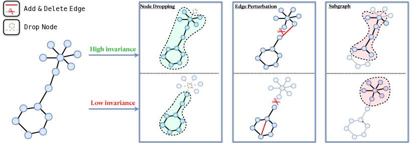
Figure 1. An illustration of the unstable invariance of current graph data augmentation strategies. The upper part of each data augmentation method shows an augmented graph that is highly invariant to the original graph, while the lower part lacks invariance to the original graph.

Data augmentation has achieved great success in image data where the invariance of various views (e.g., color-invariant, rotation-invariant, and resizing-invariant) are well-understood (chen2020simple, ; xiao2020should, ). However, due to the complex structural information and the coupling between nodes in the graph, the changes induced by the data augmentation are not easy to measure. For example, in image data, it is natural to evaluate what kind of data augmentation is more powerful (e.g., color distortion strength for color permuting (chen2020simple, )), but the situation of the graph data is much more complicated. Modifying the attributes of a node or removing an edge is not only related to the target node but also affects many other nodes (wang2020nodeaug, ), especially when GNNs follow the recursive neighborhood aggregation scheme mechanism (xu2018powerful, ). Furthermore, the importance of each node and edge in the graph is far from equivalent, which differs from the importance of pixels in image data. For example, from the node-level perspective, changing the information of key nodes will cause its neighbor nodes to be affected so seriously that their semantic labels change. However, the data augmentation requires that the neighbor nodes keep stable (xie2019unsupervised, ; you2020graph, ). From the graph-level view, removing a critical edge is enough to change a graph from a connected graph to a disconnected one, making the augmented graph and the original graph have little learnable invariance. We provide an illustration in Figure 1 to show the unstable invariance between the original graph and augmented graphs under three different data augmentation methods (Node dropping, Edge perturbation, and Subgraph sampling). The upper part of each data augmentation method shows an augmented graph that is highly invariant to the original graph, while the lower part lacks invariance to the original graph. Figure 1 shows that under the same data augmentation method, the effect of randomness on invariance is obvious and uncontrollable. Therefore, commonly used graph data augmentation methods (e.g., Node dropping, Edge perturbation, Attribute masking, and Subgraph sampling et al.) are still not well-explored and lack generalization under datasets from diverse fields. GraphCL (you2020graph, ) comes to similar conclusions after testing various data augmentation strategies. For instance, edge perturbation is more suitable for social networks but hurts biochemical molecules. In GraphCL, the composition of data augmentation strategies is an empirical process of finding the invariance suitable for the specific domains, and only a pair-wise composition of strategies can be achieved.

We propose a graph contrastive learning framework that does not composite graph data augmentation strategies based on prior domain knowledge. Because current graph data augmentation strategies fail to ensure the invariance between the augmented graph/node and the original graph/node, our framework chooses to utilize the invariance of representations learned by different GNN models for contrastive learning from a novel perspective. Specifically, different GNN models adopt their unique ”message-passing” schemes (e.g., spectral-based and spatial-based). However, the learned universal representations should be similar for the same graph/node due to the consistent structural and attribute information. Instead of learning the graph representation in a single embedding space invariant to the handcrafted augmentations, we utilize multiple GNN models to learn the representations in various embedding spaces, where the representation is invariant to the same graph/node’s representation in other embedding spaces. In essence, we regard the representations learned by each GNN model as a kind of data augmentation, and these augmented graphs are implemented through distinct embedding spaces and ”message-passing” schemes. Because no handcrafted disturbance information is injected, data augmentation based on the collaboration of multiple GNN models can ensure invariance between augmented and original graphs/nodes. Besides, the collaboration of multiple GNN models can achieve a performance similar to ensemble learning. The invariance between representations learned by multiple models can benefit the final representation learning.

We name this framework for multiple GNN models collaborative contrastive learning as Collaborative Graph Neural Networks Contrastive Learning (CGCL). CGCL is a general framework that can be appiled for training both graph-level and node-level GNN models, such as GAT (velivckovic2017graph, ), GCN (kipf2016semi, ), GIN (xu2018powerful, ), DGCNN (zhang2018end, ), and so on. CGCL working for graph-level and node-level representation learning differs slightly in that graph-level CGCL is based on batch-wise contrastive learning, whereas node-level CGCL employs a graph-wise mechanism. We validate the performance of CGCL on both graph classification tasks and node classification tasks over 12 benchmark graph datasets (9 for graph-level learning, 3 for node-level learning). Compared with the graph contrastive learning with data augmentation composition (you2020graph, ), CGCL demonstrates better generalization on various datasets and achieves better results without a handcrafted data augmentation composition. Experimental results reflect that existing data augmentation composition may be unnecessary for graph contrastive learning. Because augmenting the graph data induces a significant amount of noise, the performance improvement of the representation learning is unstable and varies across datasets.

The contributions of our work are summarized as follows:

• We propose a novel collaborative graph neural networks contrastive learning framework (CGCL) to reinforce unsupervised graph representation learning. CGCL requires no handcrafted data augmentation and composition compared with other graph contrastive learning methods.

• CGCL can work on both graph-level and node-level learning and show better generalization across different domains of datasets. The collaboration of multiple GNNs empowers CGCL with the benefits such as ensemble learning, which enable to learn better representations.

• Extensive experiments show that CGCL has advantages in graph classification tasks and node classification tasks with unsupervised learning. In addition, we present the theoretical and empirical analysis of the performance of collaboration between different GNN models.

2. Related Work

2.1. Graph Representation Learning

Graph representation learning has become a critical topic (chen2020graph, ) due to the ubiquity of graphs in real-world scenarios. As a data type containing rich structural information, many research works (grover2016node2vec, ; TQWZYM15, ; WCWPZY17, ) embed the graphs purely based on the structure. Node2vec (grover2016node2vec, ) learns a mapping of nodes to a low-dimensional space of features that maximizes the likelihood of preserving network neighborhoods of nodes. LINE (TQWZYM15, ) optimizes a carefully designed objective function that preserves both the local and global graph structures. Wang et al. (WCWPZY17, ) attempt to retrieve structural information through matrix factorization incorporating the community structure. In the recent past, graph neural networks (velivckovic2017graph, ; kipf2016semi, ; hamilton2017inductive, ; sun2019infograph, ; ying2018hierarchical, ; ren2021label, ) have shown awe-inspiring capabilities in graph representation learning, which aggregate the neighbors’ information through neural networks to learn the latent representations (xu2018powerful, ). Kipf et al. (kipf2016semi, ) propose Graph Convolutional Network (GCN) that extends convolution to graphs by a novel Fourier transformation. Graph Attention Network (GAT) (velivckovic2017graph, ) first imports the attention mechanism into graphs. Due to insufficient labeled data and out-of-distribution samples in training data, unsupervised graph representation learning gradually attracts researchers’ attention. DGI (velivckovic2018deep, ) is a general GNN for learning node representations in an unsupervised manner, which relies on maximizing mutual information between patch representations and corresponding high-level summaries of graphs. HDGI (ren2019heterogeneous, ) extends the mutual information maximization-based mechanism to the heterogeneous graph representation learning. InfoGraph (sun2019infograph, ) extends the mutual information maximization to graph-level representations. Besides, several models (hu2020gpt, ; hu2019strategies, ) work for pre-training in graph-structured data can help learn graph representations without labeled data.

2.2. Contrastive Learning

Contrastive learning has been used for unsupervised learning in vast fields, including natural language processing (radford2019language, ; devlin2018bert, ) and visual representation (chen2020simple, ; wu2018unsupervised, ; he2020momentum, ), by training an encoder that can capture similarity from data. The contrastive loss is usually a scoring function that increases the score on the single matched instance and decreases the score on multiple unmatched instances (oord2018representation, ; wu2018unsupervised, ). In the graph domain, GCC (qiu2020gcc, ) utilizes contrastive learning to pre-train a model that can serve for the downstream graph classification task by fine-tuning. LCGNN (ren2021label, ) designs a label contrastive loss to implement the contrastive learning under the guide of graph labels. GraphCL (you2020graph, ) introduces data augmentation strategies for graph contrastive learning. The contrastive learning between augmented graphs can help improve the learned graph representations. Compared to GraphCL, our proposed method learns graph/node representations through collaborative contrastive learning between different GNN models instead of between manually augmented graphs.

2.3. Data Augmentation

In visual representation learning, data augmentation has been widely applied in both supervised and unsupervised methods (bachman2019learning, ; henaff2020data, ; chen2020simple, ). The augmented data can be utilized to define contrastive prediction tasks, including global-to-local view prediction (bachman2019learning, ), neighboring view prediction (henaff2020data, ) and so on. Chen et al. (chen2020simple, ) perform simple random cropping to avoid changing the architecture when defining the contrastive prediction. The current works on graph data augmentation are relatively limited. Graph$S_{GAN}$ (ding2018semi, ) generates fake samples in low-density areas between subgraphs as augmented data and discriminates fake samples from the real in an adversarial way. Adversarial perturbations are generated to augment node features in (deng2019batch, ). NodeAug (wang2020nodeaug, ) regularizes the model prediction to ensure invariance when the data augmentation strategies induce changes. GraphCL (you2020graph, ) systematically investigates the impact of various handcrafted graph data augmentation compositions on graph representation learning. Current graph data augmentation methods primarily rely on injecting handcrafted perturbation into the graph-structured data, whereas CGCL proposed in this paper utilizes different graph encoder observation views of graph-structured data as a data augmentation method.

3. Methodology

In this section, we elaborate on the collaborative graph neural networks contrastive learning (CGCL) framework in detail for both graph-level and node-level representation learning. CGCL employs multiple GNN models as the graph encoders. Each of them works as a graph data augmentation function for other GNN models to improve the quality of learned representations. Each GNN model in CGCL updates its parameters through the contrastive learning (chen2020simple, ) between its learned representation and other GNN models’ outputs. We provide the preliminaries about unsupervised graph-level and node-level representation learning first.

3.1. Preliminaries

The goal of unsupervised graph-level representation learning is to embed the entire graph into a low-dimensional vector. In comparison, node-level representation learning aims at learning the low-dimensional representation of each node. Both of them require no label information during the learning process. Formally, we define them as follows:

Unsupervised Graph-level Representation Learning Given a set of graphs $\mathbb{G}=\{\mathcal{G}_{1},\mathcal{G}_{2},\dots\}$. The task is to learn a $d$-dimensional representation for each $\mathcal{G}_{i}\in\mathbb{G}$. Here $d$ is the pre-defined value indicating the number of dimensions of learned graph representations.

Unsupervised Node-level Representation Learning Given a graph $\mathcal{G}=(\mathcal{V},\mathcal{E})$ and the initial feature matrix of all nodes $\bm{X}\in\mathbb{R}^{|\mathcal{V}|\times D}$, and $D$ is the dimension of initial features. The unsupervised node-level representation learning is to learn the low dimensional node representations $\bm{H}\in\mathbb{R}^{|\mathcal{V}|\times d}$ that contains both structural information of $\mathcal{G}$ and node attributes from $\bm{X}$. Here, $d$ is the number of dimensions of node representations.

In the following section, we introduce CGCL handing two tasks, respectively.

3.2. CGCL for Graph-level Learning

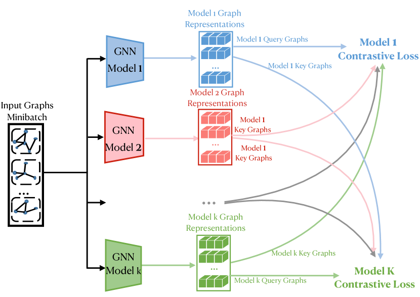
Figure 2. CGCL for graph-level representation learning. GNN Model 1, 2, $\cdots$, k are different types of graph neural networks. The minibatch graphs are embedded by them and obtain low-dimentional representations. In order to optimize the corresponding GNN model, a contrastive loss is calculated for each GNN model. For instance, GNN Model 1 uses representations learned by itself as query graphs and representations learned by all other GNN models as key graphs to compute Model 1 contrastive loss.

3.2.1. Framework Overview

We show in Figure 2 the overall framework of CGCL in processing graph-level representation learning task. The GNN models $\{\mathit{M}_{1},\mathit{M}_{2},\dots,\mathit{M}_{k}\}$ used by CGCL as graph encoders are able to encode entire graphs, and the output is the representation of each graph. The graph representations learned by $\mathit{M}_{i}$ are utilized by $\{\mathit{M}_{1},\mathit{M}_{2},\dots,\mathit{M}_{i-1},\mathit{M}_{i+1},\dots,\mathit{M}_{k}\}$ as graph data augmentations. A contrastive loss for each GNN model is defined to enforce the invariance between the positive pairs, which we will define in Section 3.2.4. Each GNN model can be updated based on the defined contrastive loss. After learning, each trained GNN model can work for graph representation learning when taking a graph as input.

3.2.2. GNN-based graph encoder

Given a set of graphs, CGCL needs to encode them into vectorized representations. Graph neural networks (GNNs) (velivckovic2017graph, ; kipf2016semi, ; hamilton2017inductive, ) have demonstrate their outstanding ability in encoding graph-structured data. In CGCL, we mainly consider GNNs as graph encoders. GNNs follow the recursive neighborhood aggregation (”message-passing”) scheme (xu2018powerful, ) to encode the node’s structural and attribute information. Given a graph $\mathcal{G}=(\mathcal{V},\mathcal{E})$ and the initial feature matrix of all nodes $\bm{X}$. The aggregation process at the $l$-th layer of a GNN can be represented as:

(1) $$\bm{a}_{n}^{(l)}=\text{AGGREGATION }^{(l)}\left(\left\{\bm{h}_{n^{\prime}}^{(l-1)}:n^{\prime}\in\mathcal{N}(n)\right\}\right),$$

$$\bm{h}_{n}^{(l)}=\text{COMBINE}^{(l)}\left(\bm{h}_{n}^{(l-1)},\bm{a}_{n}^{(l)}\right)$$

Here, $\bm{h}_{n}^{(l-1)}$ is the representation of node $n$ at the $(l-1)$-th layer with $\bm{h}_{n}^{(0)}=\bm{X}[n,:]^{T}$, and $\mathcal{N}(n)$ is the set of neighboring nodes of node $n$. The difference between each GNN is mainly reflected in the use of unique $\text{AGGREGATION}(\cdot)$ and $\text{COMBINE}(\cdot)$ functions, which define the ”message-passing” schemes. For the graph-level representation learning tasks, GNNs need an extra $\text{READOUT}(\cdot)$ to summarize the representation of $\mathcal{G}$ from node representations:

(2) $$h_{\mathcal{G}}=\operatorname{READOUT}\left(\left\{\bm{h}_{n}^{(l)}:v_{n}\in\mathcal{V},l\in L\right\}\right)$$

The key to CGCL is to choose various GNNs for collaborative learning. Technically, any GNN working on graph-level tasks can be used as one of the graph encoders here. However, the collaborations of different types of GNNs have a significant impact on the performance of CGCL. We analyze the GNN models selection in Section 4.2.3 from experimental results. Here, we propose three empirical insights first:

• The difference between the embedding spaces of various GNNS is uneven. The performance of the collaboration is harmed when there are too many or too few disparities.

• The $\operatorname{READOUT}$ (pooling) method has a significant influence on the graph-level representation. In the supervised learning, pooling methods are strongly sensitive to the specific task, but the selected pooling method may not be suitable for unsupervised representation learning.

• Employing more GNNs as graph encoders can help achieve better performance. This is equivalent to learning more essential invariance from multi-view representations.

For graph-level representation learning, the graph encoder candidates include GIN (xu2018powerful, ), GAT (velivckovic2017graph, ), GCN (kipf2016semi, ), and DGCNN (zhang2018end, ) in this paper. They can be combined for collaboration with CGCL. It should be noted that the $\operatorname{READOUT}$ of each model should be unified (e.g., global add pooling) instead of using the default method in the original work.

3.2.3. Graph representation as the data augmentation

The graph representations learned by different GNNs essentially act the data augmentation in CGCL. However, the data augmentation mechanism used here differs from that of GraphCL (you2020graph, ), which is designed manually based on priors of graph-structured data. CGCL achieves this kind of data augmentation through different ”message-passing” schemes, equivalent to observing a graph from multiple views. We provide the detailed analysis of this insight in Section 3.4 in a theoretical way.

3.2.4. Batch-wise contrastive loss

For graph-level learning, we utilize the training batch to conduct contrastive learning. Given a minibatch of $N$ graphs $\{\mathcal{G}_{1},\mathcal{G}_{2},\dots,\mathcal{G}_{N}\}$ as the input of $k$ GNN models $\{\mathit{M}_{1},\mathit{M}_{2},\dots,\mathit{M}_{k}\}$. Contrastive learning can be considered as learning an encoder for a dictionary look-up task (he2020momentum, ). We take $\mathit{M}_{1}$ as an example. The representations $\{\bm{h}^{\mathit{M}_{1}}_{\mathcal{G}_{1}},\bm{h}^{\mathit{M}_{1}}_{\mathcal{G}_{2}},\dots,\bm{h}^{\mathit{M}_{1}}_{\mathcal{G}_{N}}\}$ learned by $\mathit{M}_{1}$ act as query graphs, while the representations learned by other models are key graphs. Between query and key graphs, the positive graph representation pairs are:

(3) $$\{(\bm{h}^{\mathit{M}_{1}}_{\mathcal{G}_{i}},\bm{h}^{\mathit{M}_{j}}_{\mathcal{G}_{i}})\ |\ i\in[1,N],j\in[2,k]\}$$

Therefore, each graph encoded by $\mathit{M}_{1}$ has $k-1$ positive samples. In essence, the positive graph pair indicates the representations of the same graph but learned by different graph encoders. Meanwhile, the other pairs are negative. Here, we utilize the InfoNCE (oord2018representation, ) to calculate the contrastive loss for each graph encoder. We define the contrastive loss between two graph encoders $\mathit{M}_{p}$ and $\mathit{M}_{q}$ first, so the contrastive loss $\mathcal{L}_{\mathit{M}_{p}}(\mathit{M}_{q})$ can be represented as:

(4) $$\mathcal{L}_{\mathit{M}_{p}}(\mathit{M}_{q})=-\sum_{j=1}^{N}\log\frac{\exp\left(\bm{h}^{\mathit{M}_{p}}_{\mathcal{G}_{j}}\cdot\bm{h}^{\mathit{M}_{q}}_{\mathcal{G}_{j}}/\tau\right)}{\sum_{n=1}^{N}\exp\left(\bm{h}^{\mathit{M}_{p}}_{\mathcal{G}_{j}}\cdot\bm{h}^{\mathit{M}_{q}}_{\mathcal{G}_{n}}/\tau\right)}$$

Here, $\tau$ is the temperature hyper-parameter that controls the concentration level of the distribution (hinton2015distilling, ). In this contrastive loss, $\mathit{M}_{p}$ acts as the query encoder (i.e., providing query graphs), while $\mathit{M}_{q}$ provides key graphs as data augmentation. When considering all collaborative graph encoders, the contrastive loss of $\mathit{M}_{p}$ can be denoted as:

(5) $$\mathcal{L}_{\mathit{M}_{p}}=\sum_{\mathit{M}_{q}\in\{\mathit{M}_{i}\}_{i=1}^{k}\setminus{\mathit{M}_{p}}}\mathcal{L}_{\mathit{M}_{p}}(\mathit{M}_{q})$$

$\mathit{M}_{p}$ can be updated based on the contrastive loss $\mathcal{L}_{\mathit{M}_{p}}$ through back-propagation. Other GNNs follow the same process to compute their own contrastive loss and get updated through minibatch training iteratively. The detailed collaborative learning process of CGCL is described in Algorithm 1.

3.2.5. CGCL helps GNN pre-training

CGCL does not rely on specific tasks labels so that helps the pre-training of the GNN. The GNNs trained through CGCL can embed the graph data universally. For specific downstream tasks, the trained GNNs can be finetuned in an end-to-end manner, which can help overcome the challenges of scarce task-specific labeled data and out-of-distribution samples in training set (hu2019strategies, ).

Discussion Several existing contrastive learning models (he2020momentum, ; ren2021label, ; wu2018unsupervised, ) choose to maintain a memory bank, which can break the contraints from batch size. The memory bank needs to have a large size and keeps consistent. He et al. (he2020momentum, ) design a momentum-based update rule to keep the memory bank consistent with low cost. However, the momentum-based update rule works for the scenario where the query encoder and key encoder can share parameters. In addition, in CGCL, the optimization process of selected GNNs will be divergent, so if the representations from the previous batch is saved in the memory bank for contrastive learning, the inconsistency problem becomes more serious. Therefore, we drop the memory bank in CGCL, but adopt batch-wise learning.

It is also worth discussing that the idea of CGCL is close to ensemble learning (zhou2009ensemble, ), which helps improve machine learning results by combining multiple models. As the meta-algorithms, traditional ensemble methods work on combining several machine learning techniques into one predictive model in order to decrease variance (e.g., Bagging) and bias (e.g., Boosting) (zhou2002ensembling, ). Think back to CGCL, each graph encoder utilizes their unique ”message-passing” scheme to analyze the graph data, while CGCL contributes to eliminate the variance and bias between the same graph’s representation from different graph encoders and promote them to reach a consensus. For unsupervised graph representation learning, the contrastive loss can indicate this consensus and guide the ensemble learning process.

Algorithm 1 Collaborative Graph Neural Networks Contrastive Learning

1:The set of gnn-based graph encoders $\{\mathit{M}_{i}\}_{i=1}^{k}$; Batch size $N$; Temperature; parameter $\tau$

2:Trained graph neural networks $\{\mathit{M}_{i}\}_{i=1}^{k}$;

3:for all sampled graph minibatch $\{\mathcal{G}_{j}\}_{j=1}^{N}$ do

4:    for $j\in\{1,\dots,N\}$ do

5:       for all $\mathit{M}_{i}\in\{\mathit{M}_{i}\}_{i=1}^{k}$ do

6:          $\bm{h}^{\mathit{M}_{i}}_{\mathcal{G}_{j}}=\mathit{M}_{i}(\mathcal{G}_{j})$       //Encoding the input graph

7:       end for

8:    end for

9:    for all $\mathit{M}_{p}\in\{\mathit{M}_{i}\}_{i=1}^{k}$ do

10:       for all $\mathit{M}_{q}\in\{\mathit{M}_{i}\}_{i=1}^{k}\setminus{\mathit{M}_{p}}$ do

11:          define contrastive loss between two encoders:

12:          $\mathcal{L}_{\mathit{M}_{p}}(\mathit{M}_{q})=-\sum_{j=1}^{N}\log\frac{\exp\left(\bm{h}^{\mathit{M}_{p}}_{\mathcal{G}_{j}}\cdot\bm{h}^{\mathit{M}_{q}}_{\mathcal{G}_{j}}/\tau\right)}{\sum_{n=1}^{N}\exp\left(\bm{h}^{\mathit{M}_{p}}_{\mathcal{G}_{j}}\cdot\bm{h}^{\mathit{M}_{q}}_{\mathcal{G}_{n}}/\tau\right)}$;

13:       end for

14:       $\mathcal{L}_{\mathit{M}_{p}}=\displaystyle\sum_{\mathit{M}_{q}\in\{\mathit{M}_{i}\}_{i=1}^{k}\setminus{\mathit{M}_{p}}}\mathcal{L}_{\mathit{M}_{p}}(\mathit{M}_{q})$

15:       update graph encoder $\mathit{M}_{p}$ to minimize $\mathcal{L}_{\mathit{M}_{p}}$

16:    end for

17:end for

18:return graph neural networks $\{\mathit{M}_{i}\}_{i=1}^{k}$;

3.3. CGCL for Node-level Learning

3.3.1. Framework Overview

The main difference for node-level learning is that the representation learning of nodes requires all nodes in the same graph as input for GNN-based graph encoders and cannot be randomly divided into batches because of node dependence (bai2021ripple, ). Therefore, CGCL employs graph-wise contrastive learning for node-level representation learning, which means the contrastive loss is computed within each complete graph.

3.3.2. Graph-wise contrastive loss

Given a graph $\mathcal{G}=(\mathcal{V},\mathcal{E})$ and the initial feature matrix $\bm{X}$ as the input of $k$ node-level GNN models $\{\mathit{M}_{1},\mathit{M}_{2},\dots,\mathit{M}_{k}\}$. Taking $\mathit{M}_{p}$ as an example, node representations $\{\bm{h}^{\mathit{M}_{1}}_{{v}_{1}},\bm{h}^{\mathit{M}_{1}}_{{v}_{2}},\dots,\bm{h}^{\mathit{M}_{1}}_{{v}_{|\mathcal{V}|}}\}$ learned by it based on Equation 1 are query nodes, where $v\in\mathcal{V}$. The node representations learned by another model $\mathit{M}_{q}$ serve as key nodes. The contrastive loss between $\mathit{M}_{p}$ and $\mathit{M}_{q}$ within the graph $\mathcal{G}$ is:

(6) $$\mathcal{L}_{\mathit{M}_{p}}(\mathit{M}_{q},\mathcal{G})=-\sum_{j=1}^{|\mathcal{V}|}\log\frac{\exp\left(\bm{h}^{\mathit{M}_{p}}_{v_{j}}\cdot\bm{h}^{\mathit{M}_{q}}_{v_{j}}/\tau\right)}{\sum_{n=1}^{|\mathcal{V}|}\exp\left(\bm{h}^{\mathit{M}_{p}}_{v_{j}}\cdot\bm{h}^{\mathit{M}_{q}}_{v_{n}}/\tau\right)}$$

Considering all graph encoder, the contrastive loss of $\mathit{M}_{p}$ can be calculated similar to Equation 5:

(7) $$\mathcal{L}_{\mathit{M}_{p}}(\mathcal{G})=\sum_{\mathit{M}_{q}\in\{\mathit{M}_{i}\}_{i=1}^{k}\setminus{\mathit{M}_{p}}}\mathcal{L}_{\mathit{M}_{p}}(\mathit{M}_{q},\mathcal{G})$$

The contrastive loss can be computed for the datasets containing multiple graphs by summing the loss on all graphs. Each model can be updated by their contrastive loss, and the node representations learned by each model will reach a consensus finally.

Table 1. Graph classification accuracy on all datasets. We use bold $\color[rgb]{1,0,0}{red}$ number to denote the best result on each dataset.

	Methods	NCI1	PROTEINS	D$\&$D	MUTAG	COLLAB	IMDB-B	IMDB-M	RDT-B	RDT-M
Kernels	WL	76.65$\pm$1.99	72.92$\pm$0.56	76.44$\pm$2.35	80.72$\pm$3.00	-	72.30$\pm$3.44	46.95$\pm$0.46	68.82$\pm$0.41	46.06$\pm$0.21
	GL	62.48$\pm$2.11	72.23$\pm$4.49	72.54$\pm$3.83	81.66$\pm$2.11	72.84$\pm$0.28	65.87$\pm$0.98	-	77.34$\pm$0.18	41.01$\pm$0.17
	DGK	80.31$\pm$0.46	73.30$\pm$0.82	71.12$\pm$0.21	87.44$\pm$2.72	73.09$\pm$0.25	66.96$\pm$0.56	44.55$\pm$0.52	78.04$\pm$0.39	41.27$\pm$ 0.18
Graph	Node2vec	54.89$\pm$1.61	57.49$\pm$3.57	67.12$\pm$4.32	72.63$\pm$10.20	-	61.03$\pm$7.13	-	-	-
Embed	Sub2vec	52.84$\pm$1.47	53.03$\pm$5.55	59.34$\pm$8.01	61.05$\pm$15.80	-	55.26$\pm$1.54	36.67$\pm$0.83	71.48$\pm$0.41	36.68$\pm$0.42
	Graph2vec	73.22$\pm$1.81	73.30$\pm$2.05	71.98$\pm$3.54	83.15$\pm$9.25	-	71.10$\pm$0.54	50.44$\pm$0.87	75.78$\pm$1.03	47.86$\pm$0.26
GNNs	InfoGraph	76.20$\pm$1.06	74.44$\pm$0.31	72.85$\pm$1.78	89.01$\pm$1.13	70.65$\pm$1.13	73.03$\pm$0.87	49.69$\pm$0.53	82.50$\pm$1.42	53.46$\pm$1.03
	${GCC}_{freeze}$	66.33$\pm$2.65	74.48$\pm$3.12	75.63$\pm$3.22	68.11$\pm$2.78	78.9	72	49.4	89.8	53.7
	GraphCL	77.87$\pm$0.41	74.39$\pm$0.45	78.62$\pm$0.40	86.80$\pm$1.34	71.36$\pm$1.15	71.14$\pm$0.44	-	89.53$\pm$0.84	55.99$\pm$0.28
Proposed	${\textsc{CGCL}}_{GIN}$	77.89$\pm$0.54	76.28$\pm$0.31	79.37$\pm$0.47	89.05$\pm$1.42	73.28$\pm$2.12	73.11$\pm$0.74	51.73$\pm$1.37	91.31$\pm$1.22	54.47$\pm$1.08

3.4. Theoretical Analysis of CGCL

You et al. (you2020graph, ) build a bridge between the contrastive loss and mutual information maximization, which can help depict the essence of contrastive learning. We follow a similar way to analyze CGCL. For simplicity, we analyze CGCL with two graph encoders $\mathit{M}_{p}$ and $\mathit{M}_{q}$. For one sampled graph minibatch $\{\mathcal{G}_{j}\}_{j=1}^{N}$, the CGCL loss can be rewritten as:

(8) $$\mathcal{L}_{\mathit{M}_{p}}(\mathit{M}_{q}) =-\sum_{j=1}^{N}\log\frac{\exp\left(\bm{h}^{\mathit{M}_{p}}_{\mathcal{G}_{j}}\cdot\bm{h}^{\mathit{M}_{q}}_{\mathcal{G}_{j}}/\tau\right)}{\sum_{n=1}^{N}\exp\left(\bm{h}^{\mathit{M}_{p}}_{\mathcal{G}_{j}}\cdot\bm{h}^{\mathit{M}_{q}}_{\mathcal{G}_{n}}/\tau\right)}$$

$$=-\sum_{j=1}^{N}\left[\bm{h}^{\mathit{M}_{p}}_{\mathcal{G}_{j}}\cdot\bm{h}^{\mathit{M}_{q}}_{\mathcal{G}_{j}}/\tau-\log\left(\sum_{n=1}^{N}\exp\left(\bm{h}^{\mathit{M}_{p}}_{\mathcal{G}_{j}}\cdot\bm{h}^{\mathit{M}_{q}}_{\mathcal{G}_{n}}/\tau\right)\right)\right]$$

$$=-\sum_{j=1}^{N}\frac{f_{\mathit{M}_{p}}(\mathcal{G}_{j})\cdot f_{\mathit{M}_{q}}(\mathcal{G}_{j})}{\tau}+\sum_{j=1}^{N}\log\left(\sum_{n=1}^{N}\exp\left(\frac{f_{\mathit{M}_{p}}(\mathcal{G}_{j})\cdot f_{\mathit{M}_{q}}(\mathcal{G}_{n})}{\tau}\right)\right)$$

Here, $f_{\mathit{M}_{p}}(\cdot)$ and $f_{\mathit{M}_{q}}(\cdot)$ are graph encoders $\mathit{M}_{p}$ and $\mathit{M}_{q}$, respectively. We continue to write the Equation 8 as the expectation form:

(9) $$\mathcal{L}_{\mathit{M}_{p}}(\mathit{M}_{q})= -N\mathbb{E}_{\mathbb{P}_{(f_{\mathit{M}_{p}}(\mathcal{G}),f_{\mathit{M}_{q}}(\mathcal{G}))}}\frac{f_{\mathit{M}_{p}}(\mathcal{G})\cdot f_{\mathit{M}_{q}}(\mathcal{G})}{\tau}$$

$$+N\mathbb{E}_{f_{\mathit{M}_{p}}(\mathcal{G})}\log(\mathbb{E}_{f_{\mathit{M}_{q}}(\mathcal{G})}\exp(\frac{f_{\mathit{M}_{p}}(\mathcal{G})\cdot f_{\mathit{M}_{q}}(\mathcal{G})}{\tau}))+N\log N$$

$$= N\mathbb{E}_{\mathbb{P}_{f_{\mathit{M}_{p}}(\mathcal{G})}}\{-\mathbb{E}_{\mathbb{P}_{(f_{\mathit{M}_{q}}(\mathcal{G})\mid f_{\mathit{M}_{p}}(\mathcal{G}))}}\frac{f_{\mathit{M}_{p}}(\mathcal{G})\cdot f_{\mathit{M}_{q}}(\mathcal{G})}{\tau}$$

$$+\log(\mathbb{E}_{\mathbb{P}_{f_{\mathit{M}_{q}}(\mathcal{G})}}\exp(\frac{f_{\mathit{M}_{p}}(\mathcal{G})\cdot f_{\mathit{M}_{q}}(\mathcal{G})}{\tau}))\}+N\log N$$

We ignore the last term $N\log N$ and the multiplier $N$, and the loss can be represented in the form:

(10) $$\mathcal{L}=\mathbb{E}_{\mathbb{P}_{f_{\mathit{M}_{p}}(\mathcal{G})}}\{ -\mathbb{E}_{\mathbb{P}_{(f_{\mathit{M}_{q}}(\mathcal{G})\mid f_{\mathit{M}_{p}}(\mathcal{G}))}}T(f_{\mathit{M}_{p}}(\mathcal{G}),f_{\mathit{M}_{q}}(\mathcal{G}))$$

$$+\log(\mathbb{E}_{\mathbb{P}_{f_{\mathit{M}_{q}}(\mathcal{G})}}e^{T(f_{\mathit{M}_{p}}(\mathcal{G}),f_{\mathit{M}_{q}}(\mathcal{G}))})\}$$

Here, $\mathbb{P}_{(f_{\mathit{M}_{p}}(\mathcal{G}),f_{\mathit{M}_{q}}(\mathcal{G}))},\mathbb{P}_{(f_{\mathit{M}_{q}}(\mathcal{G})\mid f_{\mathit{M}_{p}}(\mathcal{G}))},\mathbb{P}_{f_{\mathit{M}_{p}}(\mathcal{G})}$ are respectively the joint, conditional and marginal distribution of graph representations from two graph encoders, and $T(\cdot,\cdot)$ is a learnable score function which we apply the inner product together with temperature factor $\tau$. Based on the conclusion from Hjelm et al. (hjelm2018learning, ), optimizing Equation 10 is equivalent to maximizing a lower bound of the mutual information between the representations $\bm{h}^{\mathit{M}_{p}}_{\mathcal{G}}=f_{\mathit{M}_{p}}(\mathcal{G})$, $\bm{h}^{\mathit{M}_{q}}_{\mathcal{G}}=f_{\mathit{M}_{q}}(\mathcal{G})$ of the same graph $\mathcal{G}$ learned by two graph encoders.

GraphCL (you2020graph, ) defines a general framework for existing graph contrastive learning methods, where the general loss can be formulated as:

(11) $$\mathcal{L}=\mathbb{E}_{\mathbb{P}_{\hat{\mathcal{G}}_{i}}}\{-\mathbb{E}_{\mathbb{P}_{(\mathcal{G}_{j}\mid\hat{\mathcal{G}}_{i})}}T(f_{1}(\hat{\mathcal{G}}_{i}),f_{2}(\hat{\mathcal{G}}_{j}))+\log(\mathbb{E}_{\mathbb{P}_{\hat{\mathcal{G}}_{j}}}e^{T(f_{1}(\hat{\mathcal{G}}_{i}),f_{2}(\hat{\mathcal{G}}_{j}))})\}$$

It reflects that the contrastive learning equals to maximizing a lower bound of the mutual information between two views: $(f_{1},\hat{\mathcal{G}}_{i})$ and $(f_{2},\hat{\mathcal{G}}_{j})$. GraphCL chooses to define $f_{1}=f_{2}$, but maximizes the mutual information between $\hat{\mathcal{G}}_{i}$ and $\hat{\mathcal{G}}_{j}$ generated by handcrafted data augmentation. However, according to our analysis in Section 1, the data augmentation methods on the graph cannot stably guarantee the invariance between augmented graphs, so it may not be reasonable to maximize the mutual information between the augmented graph data. CGCL chooses to utilize $f_{1}\neq f_{2}$ and $\hat{\mathcal{G}}_{i}=\hat{\mathcal{G}}_{j}=\mathcal{G}$ to define two views. From this perspective, the meaning of data augmentation provided by different GNN models claimed in Section 3.2.3 can be well-understood. Since there is no unpredictable handcrafted disturbance injecting to the original graph, the invariance can be guaranteed.

4. Experiments

In this section, we first verify the effectiveness of the graph-level representations learned by CGCL in the setting of unsupervised learning and pretrain-finetune learning (you2020graph, ) in the graph classification tasks. Then we demonstrate the node representations learned by CGCL in the task of node classification (velivckovic2018deep, ). In addition, we analyze the source of the performance improvement brought by CGCL and visualize the learned node representations in Section 4.3.3. At last part, we verified the reliability of the collaboration between graph encoders through convergence analysis.

4.1. Datasets

For graph-level representation learning, we conduct experiments on 9 widely used benchmark datasets: NCI1, PROTEINS, D$\&$D, MUTAG, COLLAB, IMDB-BINARY, IMDB-MULTI, REDDIT-BINARY, REDDIT-MULTI-5K. All of them come from the benchmark TUDataset (morris2020tudataset, ). For node-level representation learning, we test CGCL on 3 well-known benchmark dataset: Cora, CiteSeer and Pubmed (sen2008collective, ). For all the above datasets, we reach them with the support of the PyTorch Geometric Library. Additional details of these datasets are in Appendix 6.1.

Table 2. Graph classification accuracy in the setting of pretrain-finetune learning on all datasets. We use bold $\color[rgb]{1,0,0}{red}$ number to denote the best result on each dataset.

Methods	NCI1	PROTEINS	D$\&$D	COLLAB	IMDB-B	IMDB-M	RDT-B	RDT-M
GAE	74.36$\pm$0.24	70.51$\pm$.17	74.54$\pm$0.68	75.09$\pm$0.19	-	-	87.69$\pm$0.40	53.58$\pm$0.13
InfoGraph	74.86$\pm$0.26	72.27$\pm$0.40	75.78$\pm$0.34	73.76$\pm$0.29	-	-	88.66$\pm$0.95	53.61$\pm$0.31
GraphCL	74.63$\pm$0.25	74.17$\pm$0.34	76.17$\pm$1.37	74.23$\pm$0.21	-	-	89.11$\pm$0.19	52.55$\pm$0.45
GCC	73.20$\pm$1.48	72.49$\pm$3.42	74.57$\pm$2.84	71.65$\pm$2.91	71.34$\pm$1.98	49.19$\pm$2.76	84.34$\pm$5.62	50.21$\pm$1.18
${\textsc{CGCL}}_{GCN}$	73.41$\pm$0.52	74.98$\pm$0.48	76.53$\pm$0.39	72.99$\pm$0.68	72.74$\pm$0.30	51.42$\pm$0.54	88.98$\pm$0.24	50.30$\pm$0.90

4.2. Graph-level Representation Learning

4.2.1. Unsupervised Graph Representation Learning

We first evaluate the representations learned by CGCL in the setting of unsupervised learning. We follow the same process of InfoGraph (sun2019infograph, ), where representations are learned by models without any labels and then fed them to a SVM from sklearn to evaluate the graph classification performance. We select three categories of models as our comparison methods:

• Kernel-based method: Weisfeiler-Lehman subtree kernel (WL) (shervashidze2011weisfeiler, ), Graphlet Kernel(GL), and Deep Graph Kernel (DGK) (yanardag2015deep, ): They first decompose graphs into sub-components based on the kernel definition, then learn graph embeddings in a feature-based manner.

• Graph embedding-based methods: Sub2vec (adhikari2018sub2vec, ), Node2vec (grover2016node2vec, ), Graph2vec (narayanan2017graph2vec, ): They extend document embedding neural networks to learn representations of entire graphs.

• Graph neural network methods: InfoGraph (sun2019infograph, ): It is an unsupervised with the pooling operator for graph representation learning base on the mutual information maximization. GCC (qiu2020gcc, ): It follows pre-training and fine-tuning paradigm for graph representation learning. GarphCL (you2020graph, ): It implements contrastive learning between augmented graphs to obtain graph representation in an unsupervised manner.

${\textsc{CGCL}}_{GIN}$ denotes GIN (xu2018powerful, ) trained under the proposed framework CGCL. The graph encoder candidates include GAT (velivckovic2017graph, ), GCN (kipf2016semi, ), and DGCNN (zhang2018end, ), which are combined with GIN to conduct collaborative contrastive learning. The representations learned by ${\textsc{CGCL}}_{GIN}$ are extracted for the downstream graph classification. We test the task ten times and report the average accuracy and the standard deviation. In our experiments, only two graph encoders or three graph encoders collaborative learning settings are used. The result of ${\textsc{CGCL}}_{GIN}$ we report in Table 1 is the best, and the results of other assembly are reported in Table 3. More detailed information about training settings can be viewed in Appendix 6.3. From the results in Table 1, CGCL achieves the best result on the six datasets. In particular, compared with GraphCL, GraphCL has an advantage in the dataset RDT-M, but not in some datasets with a low average node degree. This observation is also in line with our illustration in Figure 1, because when the graph is small and not dense enough, the perturbation from the data augmentation is more likely to damage the invariance, e.g., a greater probability of affecting the graph connectivity by dropping a single node.

4.2.2. Pretrain-Finetune Graph Representation Learning

In this setting, CGCL first conducts collaborative contrastive learning to pretrain the graph encoders. Then we use 10% labeled graph data of the whole dataset to finetune the pretrained graph encoder end-to-end for the downstream graph classification tasks. Here, we utilize GAE (kipf2016variational, ), InfoGraph (sun2019infograph, ), GCC (qiu2020gcc, ), and GraphCL (you2020graph, ) to pretrain GCN for comparison. GAE focuses on the graph structure reconstruction and InfoGraph utilizes the local-glocal mutual information maximization. GCC and GraphCL pretrain the graph encoder based on the contrastive learning between augmented graph data. CGCL employs GCN and GIN as graph encoders to fulfill the designed contrastive learning in each dataset. For fairness, we finetune GCN with 10% labeled graph and report the graph classification accuracy. More implementation details can be referred to in Appendix 6.3.2. The performance in each dataset of different methods is presented in Table 2. It can be seen from the results that CGCL has achieved the best results on four datasets, and the proposed method saves time cost in generating augmented data and exploring to composite them in an appropriate strategy.

Table 3. Graph classification accuracy on all datasets with different graph encoders assembly. The bold $\color[rgb]{1,0,0}{red}$ number denotes the best learning result of GIN on each dataset.

Dataset	assembly	GIN	GCN	GAT	DGCNN	Set2Set
PROTEINS	GIN+GCN	75.84	75.04
	GIN+DGCNN	72.5			67.85
	GIN+GAT	74.98		72.92
	GIN+Set2Set	71.44				72.76
	GIN+GCN+GAT	76.28	75.32	74.37
	GIN+GCN+DGCNN	74.03	71.76		74.37
MUTAG	GIN+GCN	87.67	84.83
	GIN+DGCNN	87.96			86.72
	GIN+GAT	88.83		85.29
	GIN+Set2Set	85.15				78.35
	GIN+GCN+GAT	86.91	85.71	84.12
	GIN+GCN+DGCNN	89.05	85.74		86.94
D$\&$D	GIN+GCN	76.13	76.16
	GIN+DGCNN	76.39			72.58
	GIN+GAT	76.35		75.97
	GIN+Set2Set	75.68				73.42
	GIN+GCN+GAT	79.37	77.21	78.18
	GIN+GCN+DGCNN	77.44	76.40		74.85

4.2.3. Graph Encoder Selection

The type and quantity of graph encoders have an important influence on collaborative contrastive learning performance. We experiment with different types and numbers of graph encoders assembly on each dataset. Based on the experimental results, we get some empirical insights as described in Section 3.2.2. Table 3 shows the results of combining two or three graph encoders on 3 datasets.

We focus on the performance of unsupervised graph representation learning of ${\textsc{CGCL}}_{GIN}$. From Table 3, we can find that the collaboration of three graph encoders is better than that of the two encoders. The phenomenon is consistent to the conclusion proposed by GraphCL (you2020graph, ), that is, the harder data augmentation benifits the performance of contrastive learning. Here, the consensus reached by more graph encoders is a kind of harder data augmentation. In addition, we find that DGCNN cannot help train GIN better through collaboration than GCN and GAT. When we analyze the structure of DGCNN, we notice that the pooling layer of DGCNN is forcibly closed to the graph classification task and needs to be trained in an end-to-end way. This ungeneralized design makes the pooling layer can not be well trained in unsupervised learning. In comparison, we assign a global add pooling layer to GAT, GCN and GIN. It also reflect that the $\operatorname{READOUT}$ method has a great influence on the graph level representation, and we should keep the graph encoder use the same pooling layer to diminish the difference of embedding spaces. Here, we additionally use a non-GNN method Set2Set (vinyals2015order, ) for comparison, and the results show that it does not collaborate well with the GNN models. The reason should also be that the embedding space is too different, which makes it difficult for the graph encoders to reach a consensus on representations.

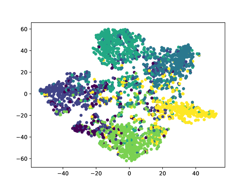
(a) GCN

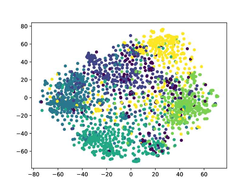
(b) DGI

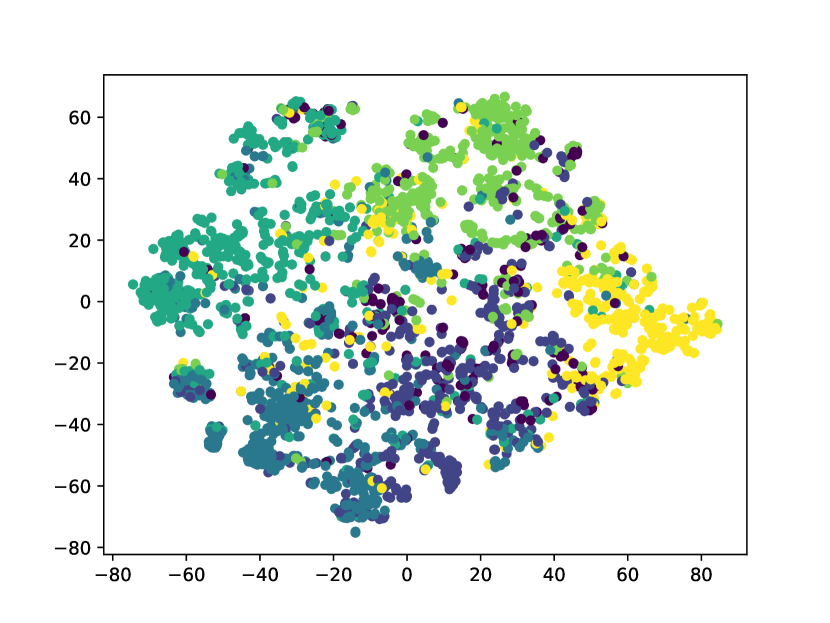
(c) ${\textsc{CGCL}}_{GCN}$

Figure 3. The learned node representations on the CiteSeer dataset visualized by t-SNE (buja1996interactive, )

4.3. Node-level Representation Learning

4.3.1. Node classification Tasks

For the effectiveness of CGCL on node-level representation learning, we use the node classification task to evaluate. The representations learned through unsupervised methods are fed into a downstream classifier. GAT and GCN are utilized as the graph encoders in CGCL. DGI (velivckovic2018deep, ) and GraphCL (you2020graph, ) are used as unsupervised comparison methods. GCN and GAT trained in a semi-supervised manner are compared with CGCL as well. We conduct the experiments on three datasets (Cora, Citeseet, and PubMed) with random splits, where 40 nodes per class from labeled nodes in the training set, 500 nodes are used as the validation set, and 1000 nodes for testing. Many existing works conduct experiments based on the standard split (kipf2016semi, ; velivckovic2018deep, ), here we have to explain why we use 40 nodes per class for training instead of 20 nodes in the standard split. Since we use contrastive learning to discriminate each node, the distribution of representations learned by CGCL is sparser than those under semi-supervised conditions. The distance between node will be larger even if nodes have the same label, so using 20 nodes are not enough to train a classifier. However, this does not mean that the representations learned by CGCL are not effective because a qualified representation is to have stronger expressive ability and distinguishability. For the sake of fairness, we apply the same settings for all methods. We run the experiments 10 times and report the mean and standard deviation of accuracy. Other detailed experimental parameters are provided in Appendix 6.4. The node classification accuracy are presented in Table 4. DGI(64) denotes that the GCN trained by DGI has the 64-dimensional hidden feature, while the original DGI in (velivckovic2018deep, ) has the 512-dimensional hidden feature. All other methods set the dimension of the hidden feature as 64. GraphCL(A+I) means that AttrMask and Identical are used for the data augmentation. N and S represent NodeDrop and Subgraph, respectively. ${\textsc{CGCL}}_{GCN}$ and ${\textsc{CGCL}}_{GAT}$ beat all unsupervised methods. For Cora and PubMed, they even surpass semi-supervised learning methods, which have labeled data in training. The results fully demonstrate that for node-level representation learning, it may not be necessary to apply handcrafted data augmentation composition for contrastive learning similar to GraphCL. The data augmentation induced by the graph encoder enables the GNN model to learn important representations from multiple views.

4.3.2. Explore Source of Performance Improvement

In order to further verify that the collaboration of different GNN models can bring performance improvements and the effectiveness of data augmentation based on graph encoders, we design the experiment using two same GNN models as graph encoders. We take two GCN and two GAT to collaborate in CGCL to work on node-level tasks. We set two kinds of initialization for them, i.e., Xavier initialization (glorot2010understanding, ) and Normal distribution initialization ($\mu$=10, $\sigma$=0). The experimental results are shown in Table 5. The ”Assembly” represents the composition of GNN with initialization methods. From the results in Table 5, it can be found that the same GNN model does not bring performance improvement because the same type of GNN learns graphs with the same ”message-passing” scheme. Even though they are initialized in different ways, no augmented graph data can be provided. In contrast, the results also demonstrate that the performance improvement of collaborative contrastive learning comes from the data augmentations that are node representations learned by different graph encoders.

4.3.3. Visualization of Learned Representations

In Figure 3, we visualize the learned representations by GCN, DGI, and ${\textsc{CGCL}}_{GCN}$ on the CiteSeer dataset by t-SNE (buja1996interactive, ). The representations of GCN are extracted from the last convolution layer. From this figure, we can find that fewer discrete nodes learned by ${\textsc{CGCL}}_{GCN}$ than DGI, and the boundaries are clearer. Compared with semi-supervised GCN, nodes with the same label in ${\textsc{CGCL}}_{GCN}$ is not as dense as GCN, but the completely overlap of nodes with different labels has eased, which is brought by discriminating each node through contrastive loss. We also present the visualization of representations on the Cora dataset in the Appendix 6.5.

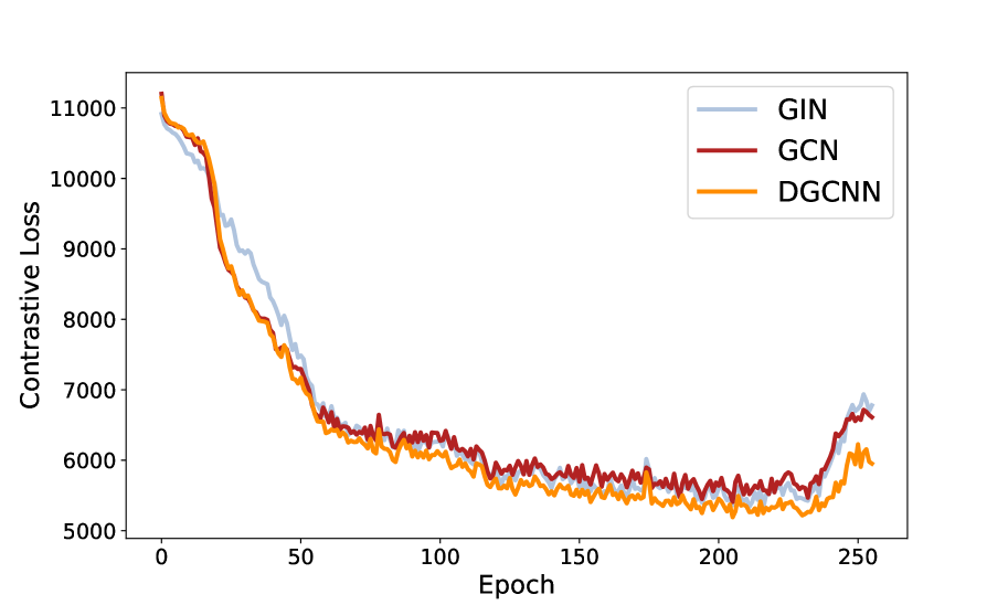
(a) GIN, GCN, and DGCNN learning in PROTEINS

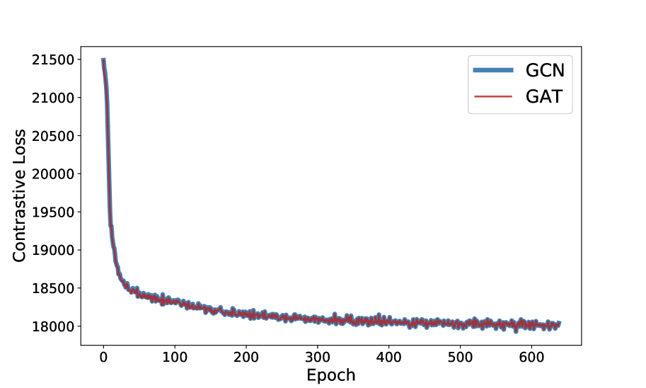
(b) GCN and GAT learning in Cora

Figure 4. Empirical convergence study of graph-level and node-level collaborative contrastive learning

4.4. Convergence Analysis

In CGCL, graph encoders compute their respective contrastive losses and optimize themself in each epoch, so we empirically analyze the convergence of this optimization process. In Figure 4, we depict the contrastive loss in graph-level and node-level representation learning, respectively. We notice that each graph encoder converges synchronously. However, for the graph-level learning, the contrastive loss rises at the end of training, so an early stop needs to be set. At node-level, contrastive learning can converge to a stable state.

Table 4. Node Classification Accuracy.

	Methods	Cora	CiteSeer	PubMed
Semi-supervised	GCN	81.71$\pm$0.46	70.07$\pm$0.21	79.06 $\pm$0.74
	GAT	82.47$\pm$0.41	72.02$\pm$0.48	79.01$\pm$0.24
Unsupervised	Raw Features	51.34$\pm$0.67	55.43$\pm$0.82	69.58$\pm$0.37
	DGI(64)	69.32$\pm$6.65	60.26$\pm$5.66	68.96$\pm$11.44
	DGI(512)	82.07$\pm$1.27	70.13$\pm$0.86	76.74$\pm$1.98
	GraphCL(A+I)	81.53$\pm$1.02	70.54$\pm$1.51	77.23$\pm$1.54
	GraphCL(N+I)	81.99$\pm$1.52	71.54$\pm$0.93	78.31$\pm$2.54
	GraphCL(S+I)	82.51$\pm$2.33	71.09$\pm$1.11	76.91$\pm$0.77
	${\textsc{CGCL}}_{GCN}$	82.34$\pm$0.98	71.84$\pm$0.47	80.66$\pm$0.69
	${\textsc{CGCL}}_{GAT}$	82.52$\pm$1.11	71.63$\pm$0.56	80.82$\pm$0.88

Table 5. Node classification accuracy when using same GNN models as graph encoders

Assembly	Initialization	Cora	CiteSeer
GCN(Normal)+GCN(Xavier)	Normal	73.0	52.9
	Xavier	71.3	45.6
GCN(Xavier)+GCN(Xavier)	Xavier	74.9	71.4
	Xavier	75.5	71.8
GCN(Normal)+GCN(Normal)	Normal	66.8	50.2
	Normal	66.9	51.2
GAT(Normal)+GAT(Xavier)	Normal	37.9	66.4
	Xavier	38.7	68.3
GAT(Xavier)+GAT(Xavier)	Xavier	27.2	68.5
	Xavier	44.7	68.7
GAT(Normal)+GAT(Normal)	Normal	44.3	70.2
	Normal	44.7	69.7

5. Conclusion

In this paper, we propose a novel collaborative graph neural networks contrastive learning framework CGCL aimed at addressing the invariance issue present in current handcrafted graph data augmentation methods. Different from manually constructing augmented graphs, CGCL uses multiple GNN-based encoders to observe the graph, and representations learned from different views are used as the augmentation of the graph-structured data. This data augmentation method avoids inducing any perturbation so that the invariance can be guaranteed. Using the contrastive learning between the graph encoders, they can reach a consensus on the graph data feature and learn the general representations in an unsupervised manner. Extensive experiments not only verify the advantages of CGCL in both unsupervised graph-level and node-level representation learning, but also demonstrate the non-necessity of handcrafted data augmentation composition for graph contrastive learning.

6. APPENDIX ON REPRODUCIBILITY

In this section, we provide detailed information of the experimental settings and configurations to ensure the reproducibility of our work.

6.1. Dataset Details

The datasets tested for graph level representation learning are describe in Table 6. The dataset used in the node-level representation learning task are listed in Table 7. We get the dataset from Pytorch Geometric library.

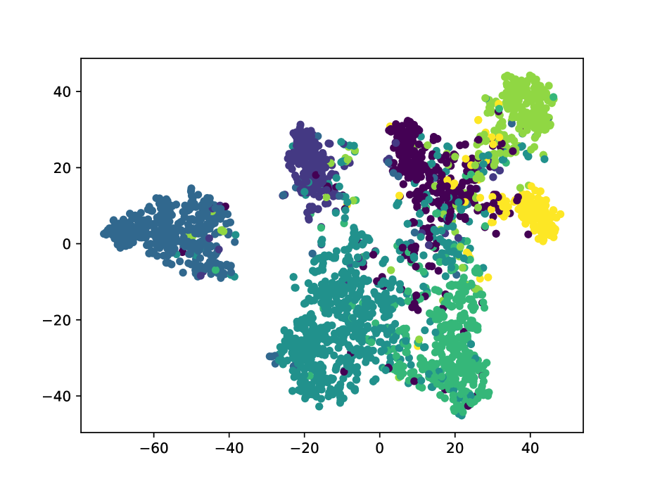
(a) GCN

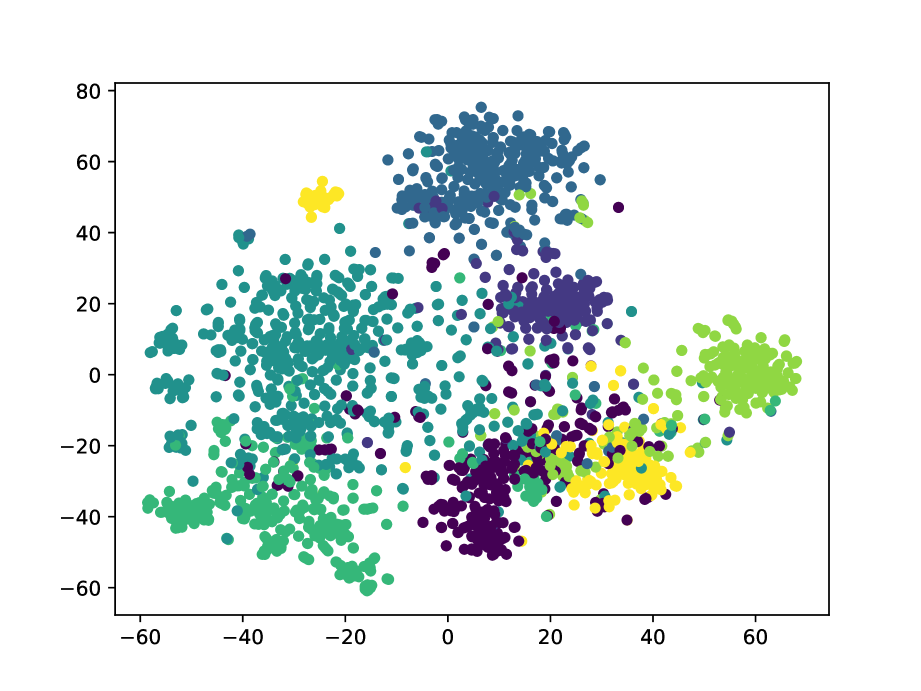
(b) DGI

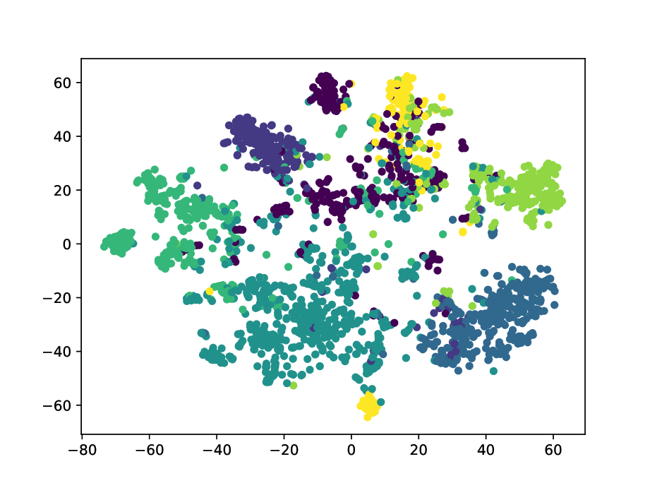
(c) ${\textsc{CGCL}}_{GCN}$

Figure 5. The learned node representations on the Cora dataset visualized by t-SNE [4]

Table 6. Detailed statistics of datasets for graph-level representation learning

Datasets	Category	Classes	Graph Num.	Avg. Node	Avg. Degree
NCI1	Biochemical Molecules	2	4110	29.87	1.08
PROTEINS	Biochemical Molecules	2	1113	39.06	1.86
D$\&$D	Biochemical Molecules	2	1178	284.32	715.66
MUTAG	Biochemical Molecules	2	188	17.93	19.79
COLLAB	Social Networks	3	5000	74.49	32.99
RDT-BINARY	Social Networks	2	2000	429.63	1.15
RDT-MULTI-5K	Social Networks	5	4999	508.52	594.87
IMDB-BINARY	Social Networks	2	1000	19.77	96.53
IMDB-MULTI	Social Networks	3	1500	13.00	65.94

Table 7. Detailed statistics of datasets for node-level representation learning

Dataset	Nodes	Edges	Classes	Attributes
Cora	2,708	5,429	7	1,433
Citeseer	3,327	4,732	6	3,703
Pubmed	19,717	44,338	3	500

6.2. Experiments Environment

We run the experiments on a Dell PowerEdge T630 Server with 2 20-core Intel CPUs and 256GB memory and the other Server with 3 GTX-1080 ti GPUs. All models are implemented in Pytorch 1.4.0, torch-geometric 1.6.0, cudatoolkit 10.1.243, and scikit-learn 0.23.1. Our code is available at: Anonymous link. The other version of code with a detailed README and exexution script will be available soon.

6.3. Settings of graph-level representation learning

6.3.1. Unsupervised graph-level representation learning

The detailed hyper-parameters used in unsupervised graph representation learning are shown in Table 8. The parameters are the same for any graph encoder assembly in the same dataset. For the classifier SVM, it searches the parameter ”C” in $\{1,10,100,1000,10000\}$.

Table 8. Hyper-parameters for unsupervised graph-level representation learning

Dataset	random seed	learning rate	weight decay	hidden size	dropout ratio	batch size	temperature	node attribute
PROTEINS	888	0.01	0.001	128	0.5	256	0.07	Default
D$\&$D	888	0.05	0.0001	128	0.5	256	0.01	Default
MUTAG	888	0.001	0.0001	128	0.5	256	0.07	Default
COLLAB	888	0.01	0.0001	128	0.5	256	0.3	Constant
RDT-BINARY	888	0.05	0.0001	128	0.5	256	0.1	Constant
RDT-MULTI-5K	888	0.05	0.0001	128	0.5	256	0.1	Constant
IMDB-BINARY	888	0.05	0.0001	128	0.5	256	0.5	OneHotDegree
IMDB-MULTI	888	0.05	0.0001	128	0.5	256	0.1	OneHotDegree

6.3.2. Pretrain-Finetune graph-level representation learning

The pretrain process uses the same hyper-parameters listed in Table 8. In finetuning step, we finetune the model with Adam optimizer, which learning rate is 0.0005 and weight decay is 0.0001. We optimize the model 120 steps. All datasets use the same hyper-parameters.

6.4. Settings of node-level representation learning

The detailed hyper-parameters used in unsupervised node representation learning are shown in Table 9. The classifier used in this task is MLP.

6.5. Visualiazation of node representations

The visualization of representations on the Cora dataset is shown in Figure 5. The results reflected on the Cora dataset are consistent with the results on CiteSeer shown in Figure 3. Nodes with the same label in ${\textsc{CGCL}}_{GCN}$ is not as dense as GCN, but the boundaries of the communities where the same label nodes exist are clearer than DGI.

Table 9. Hyper-parameters for unsupervised node-level representation learning

Dataset	random seed	learning rate	weight decay	hidden size	dropout ratio	temperature
Cora	123	0.001	0.0001	64	0.5	0.5
CiteSeer	123	0.01	0.0001	64	0.5	0.8
PubMed	123	0.01	0.0001	64	0.5	0.5

References

- [1] Bijaya Adhikari, Yao Zhang, Naren Ramakrishnan, and B Aditya Prakash. Sub2vec: Feature learning for subgraphs. In Pacific-Asia Conference on Knowledge Discovery and Data Mining, pages 170–182. Springer, 2018.
- [2] Philip Bachman, R Devon Hjelm, and William Buchwalter. Learning representations by maximizing mutual information across views. arXiv preprint arXiv:1906.00910, 2019.
- [3] Jiyang Bai, Yuxiang Ren, and Jiawei Zhang. Ripple walk training: A subgraph-based training framework for large and deep graph neural network. In 2021 International Joint Conference on Neural Networks (IJCNN), pages 1–8. IEEE, 2021.
- [4] Andreas Buja, Dianne Cook, and Deborah F Swayne. Interactive high-dimensional data visualization. Journal of computational and graphical statistics, 5(1):78–99, 1996.
- [5] Fenxiao Chen, Yun-Cheng Wang, Bin Wang, and C-C Jay Kuo. Graph representation learning: a survey. APSIPA Transactions on Signal and Information Processing, 9, 2020.
- [6] Ting Chen, Simon Kornblith, Mohammad Norouzi, and Geoffrey Hinton. A simple framework for contrastive learning of visual representations. In International conference on machine learning, pages 1597–1607. PMLR, 2020.
- [7] Zhijie Deng, Yinpeng Dong, and Jun Zhu. Batch virtual adversarial training for graph convolutional networks. arXiv preprint arXiv:1902.09192, 2019.
- [8] Jacob Devlin, Ming-Wei Chang, Kenton Lee, and Kristina Toutanova. Bert: Pre-training of deep bidirectional transformers for language understanding. arXiv preprint arXiv:1810.04805, 2018.
- [9] Ming Ding, Jie Tang, and Jie Zhang. Semi-supervised learning on graphs with generative adversarial nets. In Proceedings of the 27th ACM International Conference on Information and Knowledge Management, pages 913–922, 2018.
- [10] Xavier Glorot and Yoshua Bengio. Understanding the difficulty of training deep feedforward neural networks. In Proceedings of the thirteenth international conference on artificial intelligence and statistics, pages 249–256. JMLR Workshop and Conference Proceedings, 2010.
- [11] Aditya Grover and Jure Leskovec. node2vec: Scalable feature learning for networks. In Proceedings of the 22nd ACM SIGKDD international conference on Knowledge discovery and data mining, pages 855–864, 2016.
- [12] William L Hamilton, Rex Ying, and Jure Leskovec. Inductive representation learning on large graphs. arXiv preprint arXiv:1706.02216, 2017.
- [13] Kaiming He, Haoqi Fan, Yuxin Wu, Saining Xie, and Ross Girshick. Momentum contrast for unsupervised visual representation learning. In Proceedings of the IEEE/CVF Conference on Computer Vision and Pattern Recognition, pages 9729–9738, 2020.
- [14] Olivier Henaff. Data-efficient image recognition with contrastive predictive coding. In International Conference on Machine Learning, pages 4182–4192. PMLR, 2020.
- [15] Geoffrey Hinton, Oriol Vinyals, and Jeff Dean. Distilling the knowledge in a neural network. arXiv preprint arXiv:1503.02531, 2015.
- [16] R Devon Hjelm, Alex Fedorov, Samuel Lavoie-Marchildon, Karan Grewal, Phil Bachman, Adam Trischler, and Yoshua Bengio. Learning deep representations by mutual information estimation and maximization. arXiv preprint arXiv:1808.06670, 2018.
- [17] Weihua Hu, Bowen Liu, Joseph Gomes, Marinka Zitnik, Percy Liang, Vijay Pande, and Jure Leskovec. Strategies for pre-training graph neural networks. arXiv preprint arXiv:1905.12265, 2019.
- [18] Ziniu Hu, Yuxiao Dong, Kuansan Wang, Kai-Wei Chang, and Yizhou Sun. Gpt-gnn: Generative pre-training of graph neural networks. In Proceedings of the 26th ACM SIGKDD International Conference on Knowledge Discovery & Data Mining, pages 1857–1867, 2020.
- [19] Sergey Ivanov and Evgeny Burnaev. Anonymous walk embeddings. In International conference on machine learning, pages 2186–2195. PMLR, 2018.
- [20] Wei Jin, Tyler Derr, Haochen Liu, Yiqi Wang, Suhang Wang, Zitao Liu, and Jiliang Tang. Self-supervised learning on graphs: Deep insights and new direction. arXiv preprint arXiv:2006.10141, 2020.
- [21] Thomas N Kipf and Max Welling. Semi-supervised classification with graph convolutional networks. arXiv preprint arXiv:1609.02907, 2016.
- [22] Thomas N Kipf and Max Welling. Variational graph auto-encoders. arXiv preprint arXiv:1611.07308, 2016.
- [23] Christopher Morris, Nils M Kriege, Franka Bause, Kristian Kersting, Petra Mutzel, and Marion Neumann. Tudataset: A collection of benchmark datasets for learning with graphs. arXiv preprint arXiv:2007.08663, 2020.
- [24] Annamalai Narayanan, Mahinthan Chandramohan, Rajasekar Venkatesan, Lihui Chen, Yang Liu, and Shantanu Jaiswal. graph2vec: Learning distributed representations of graphs. arXiv preprint arXiv:1707.05005, 2017.
- [25] Aaron van den Oord, Yazhe Li, and Oriol Vinyals. Representation learning with contrastive predictive coding. arXiv preprint arXiv:1807.03748, 2018.
- [26] Jiezhong Qiu, Qibin Chen, Yuxiao Dong, Jing Zhang, Hongxia Yang, Ming Ding, Kuansan Wang, and Jie Tang. Gcc: Graph contrastive coding for graph neural network pre-training. In Proceedings of the 26th ACM SIGKDD International Conference on Knowledge Discovery & Data Mining, pages 1150–1160, 2020.
- [27] Alec Radford, Jeffrey Wu, Rewon Child, David Luan, Dario Amodei, and Ilya Sutskever. Language models are unsupervised multitask learners. OpenAI blog, 1(8):9, 2019.
- [28] Yuxiang Ren, Jiyang Bai, and Jiawei Zhang. Label contrastive coding based graph neural network for graph classification. In Database Systems for Advanced Applications, pages 123–140. Springer International Publishing, 2021.
- [29] Yuxiang Ren, Bo Liu, Chao Huang, Peng Dai, Liefeng Bo, and Jiawei Zhang. Heterogeneous deep graph infomax. arXiv preprint arXiv:1911.08538, 2019.
- [30] Yuxiang Ren, Hao Zhu, Jiawei Zhang, Peng Dai, and Liefeng Bo. Ensemfdet: An ensemble approach to fraud detection based on bipartite graph. In 2021 IEEE 37th International Conference on Data Engineering (ICDE), pages 2039–2044. IEEE, 2021.
- [31] Prithviraj Sen, Galileo Namata, Mustafa Bilgic, Lise Getoor, Brian Galligher, and Tina Eliassi-Rad. Collective classification in network data. AI magazine, 29(3):93–93, 2008.
- [32] Nino Shervashidze, Pascal Schweitzer, Erik Jan Van Leeuwen, Kurt Mehlhorn, and Karsten M Borgwardt. Weisfeiler-lehman graph kernels. Journal of Machine Learning Research, 12(9), 2011.
- [33] Chuan Shi, Yitong Li, Jiawei Zhang, Yizhou Sun, and S Yu Philip. A survey of heterogeneous information network analysis. IEEE Transactions on Knowledge and Data Engineering, 29(1):17–37, 2016.
- [34] Alexey Strokach, David Becerra, Carles Corbi-Verge, Albert Perez-Riba, and Philip M Kim. Fast and flexible protein design using deep graph neural networks. Cell Systems, 11(4):402–411, 2020.
- [35] Fan-Yun Sun, Jordan Hoffmann, Vikas Verma, and Jian Tang. Infograph: Unsupervised and semi-supervised graph-level representation learning via mutual information maximization. arXiv preprint arXiv:1908.01000, 2019.
- [36] Jian Tang, Meng Qu, Mingzhe Wang, Ming Zhang, Jun Yan, and Qiaozhu Mei. Line: Large-scale information network embedding. In Proceedings of the 24th international conference on world wide web, pages 1067–1077. International World Wide Web Conferences Steering Committee, 2015.
- [37] Petar Veličković, Guillem Cucurull, Arantxa Casanova, Adriana Romero, Pietro Lio, and Yoshua Bengio. Graph attention networks. arXiv preprint arXiv:1710.10903, 2017.
- [38] Petar Veličković, William Fedus, William L Hamilton, Pietro Liò, Yoshua Bengio, and R Devon Hjelm. Deep graph infomax. arXiv preprint arXiv:1809.10341, 2018.
- [39] Oriol Vinyals, Samy Bengio, and Manjunath Kudlur. Order matters: Sequence to sequence for sets. arXiv preprint arXiv:1511.06391, 2015.
- [40] Xiao Wang, Peng Cui, Jing Wang, Jian Pei, Wenwu Zhu, and Shiqiang Yang. Community preserving network embedding. In Thirty-First AAAI Conference on Artificial Intelligence, 2017.
- [41] Yiwei Wang, Wei Wang, Yuxuan Liang, Yujun Cai, Juncheng Liu, and Bryan Hooi. Nodeaug: Semi-supervised node classification with data augmentation. In Proceedings of the 26th ACM SIGKDD International Conference on Knowledge Discovery & Data Mining, pages 207–217, 2020.
- [42] Zhirong Wu, Yuanjun Xiong, Stella X Yu, and Dahua Lin. Unsupervised feature learning via non-parametric instance discrimination. In Proceedings of the IEEE Conference on Computer Vision and Pattern Recognition, pages 3733–3742, 2018.
- [43] Tete Xiao, Xiaolong Wang, Alexei A Efros, and Trevor Darrell. What should not be contrastive in contrastive learning. arXiv preprint arXiv:2008.05659, 2020.
- [44] Qizhe Xie, Zihang Dai, Eduard Hovy, Minh-Thang Luong, and Quoc V Le. Unsupervised data augmentation for consistency training. arXiv preprint arXiv:1904.12848, 2019.
- [45] Keyulu Xu, Weihua Hu, Jure Leskovec, and Stefanie Jegelka. How powerful are graph neural networks? arXiv preprint arXiv:1810.00826, 2018.
- [46] Pinar Yanardag and SVN Vishwanathan. Deep graph kernels. In Proceedings of the 21th ACM SIGKDD international conference on knowledge discovery and data mining, pages 1365–1374, 2015.
- [47] Zhitao Ying, Jiaxuan You, Christopher Morris, Xiang Ren, Will Hamilton, and Jure Leskovec. Hierarchical graph representation learning with differentiable pooling. In Advances in neural information processing systems, pages 4800–4810, 2018.
- [48] Yuning You, Tianlong Chen, Yongduo Sui, Ting Chen, Zhangyang Wang, and Yang Shen. Graph contrastive learning with augmentations. Advances in Neural Information Processing Systems, 33, 2020.
- [49] Yuning You, Tianlong Chen, Zhangyang Wang, and Yang Shen. When does self-supervision help graph convolutional networks? In International Conference on Machine Learning, pages 10871–10880. PMLR, 2020.
- [50] Muhan Zhang, Zhicheng Cui, Marion Neumann, and Yixin Chen. An end-to-end deep learning architecture for graph classification. In Proceedings of the AAAI Conference on Artificial Intelligence, volume 32, 2018.
- [51] Fan Zhou, Qing Yang, Ting Zhong, Dajiang Chen, and Ning Zhang. Variational graph neural networks for road traffic prediction in intelligent transportation systems. IEEE Transactions on Industrial Informatics, 2020.
- [52] Zhi-Hua Zhou. Ensemble learning. Encyclopedia of biometrics, 1:270–273, 2009.
- [53] Zhi-Hua Zhou, Jianxin Wu, and Wei Tang. Ensembling neural networks: many could be better than all. Artificial intelligence, 137(1-2):239–263, 2002.