Test of Weak Separability for Spatially Stationary Functional Field

Abstract

For spatially dependent functional data, a generalized Karhunen-Loève expansion is commonly used to decompose data into an additive form of temporal components and spatially correlated coefficients. This structure provides a convenient model to investigate the space-time interactions, but may not hold for complex spatio-temporal processes. In this work, we introduce the concept of weak separability, and propose a formal test to examine its validity for non-replicated spatially stationary functional field. The asymptotic distribution of the test statistic that adapts to potentially diverging ranks is derived by constructing lag covariance estimation, which is easy to compute for practical implementation. We demonstrate the efficacy of the proposed test via simulations and illustrate its usefulness in two real examples: China PM_2.5 data and Harvard Forest data.

Key words: Lag Covariance; Spatial Correlation; Spatial Functional Data; Weak Separability.

Short title: Test of Weak Separability

1 Introduction

Due to advances of modern sciences and technology, data with complex structures, especially those with varying temporal or/and spatial features, are more commonly collected and analyzed. Functional data analysis (FDA) has emerged as a prominent area and provides useful tools in a variety of applications, see Ramsay and Silverman (2005) for an introduction, and Hsing and Eubank (2015) for some theoretical foundations. In contrast to traditional multivariate analysis, functional data are viewed as realizations from infinite-dimensional stochastic processes or random functions, which require regularization, dimension reduction, and/or feature extraction pertaining to the modeling context. The Karhunen-Loève (KL) expansion is one of the key means for such purposes. This leads to the much-celebrated functional principal component analysis (FPCA), see Yao et al. (2005), Hall and Hosseini-Nasab (2006), Li and Hsing (2010) and the references therein. If the observed trajectories $X_{i}(t)$, $i=1,...,N$, are independently sampled from an $L^{2}$ process $X(t)\in L^{2}({\cal T})$ with the mean function $\mu(t)={\rm E}\{X_{i}(t)\}$ and covariance function $C(t_{1},t_{2})=\hbox{cov}\{X_{i}(t_{1}),X_{i}(t_{2})\}$, where ${\cal T}$ is a compact interval in $\mathbb{R}$, then the KL expansion admits $X_{i}(t)=\mu(t)+\sum_{r=1}^{\infty}\xi_{ir}\psi_{r}(t)$, where $\psi_{r}(t)$ is the $r$th eigenfunction of $C(t_{1},t_{2})$ and $\xi_{ir}=\int_{\cal T}\{X_{i}(t)-\mu(t)\}\psi_{r}(t)dt$ is the corresponding FPC score. In this model, the randomness of the process $X_{i}(t)$ is inherited by the FPC scores, i.e. projections of $X_{i}(t)$ onto the eigen-spaces, which are uncorrelated random variables whose variances are the corresponding eigenvalues $\lambda_{r}$, where $\lambda_{1}>\lambda_{2}>\cdots\geq 0$ without loss of generality (w.l.o.g.). The FPCA provides an efficient method for low-rank approximation in the sense of capturing the most variability of the processes with the least components. In practice, one may often use a few leading FPCs for adequate approximation due to rapidly decaying eigenvalues. Note that the truncation serves as a tuning balance between model parsimony and fidelity to observed data, and could depend on the sample size as well as the complexity/smoothness of the underlying process.

In recent years, there has been emerging research on dependent functional data (Hörmann et al., 2010; Paul and Peng, 2011, among others), particularly on spatial functional data (e.g. Paul and Peng, 2011; Gromenko et al., 2012; Li and Guan, 2014; Liu et al., 2017), with applications including measurements of environmental factors (temperature, precipitation, air pollutants) across monitoring stations, vegetation index at different locations, and fMRI signals in biomedical imaging. To represent the curves observed at spatial locations ${\boldsymbol{s}}_{i},i=1,\ldots,N$, a widely used model in most of the above-mentioned work is the following generalized KL expansion:

$$X({\boldsymbol{s}}_{i},t)=\mu({\boldsymbol{s}}_{i},t)+\sum_{r=1}^{\infty}\xi_{r}({\boldsymbol{s}}_{i})\psi_{r}(t),$$ (1)

where the FPC scores $\{\xi_{r}({\boldsymbol{s}}_{i})_{i=1,\dots,N;r\geq 1}\}$ are assumed to be uncorrelated across the different components for any two locations ${\boldsymbol{s}}_{i}$ and ${\boldsymbol{s}}_{i^{\prime}}$, i.e., $\hbox{cov}\{\xi_{j}({\boldsymbol{s}}_{i}),\xi_{k}({\boldsymbol{s}}_{i^{\prime}})\}=0$ for $j\not=k$. As a result, one assumes a simplified cross-covariance structure

$$C({\boldsymbol{s}}_{1},t_{1};{\boldsymbol{s}}_{2},t_{2})=\sum_{r=1}^{\infty}{\rm E}\{\xi_{r}({\boldsymbol{s}}_{1})\xi_{r}({\boldsymbol{s}}_{2})\}\psi_{r}(t_{1})\psi_{r}(t_{2}),$$ (2)

where $C({\boldsymbol{s}}_{1},t_{1};{\boldsymbol{s}}_{2},t_{2})$ is the covariance of random field $X({\boldsymbol{s}},t)\in L^{2}({\cal S}\times{\cal T})$. The covariance (2) greatly simplifies the modeling of space-time interactions. However, we emphasize that (2) requires that not only $\{\xi_{r}({\boldsymbol{s}}_{i})_{i=1,\dots,N;r\geq 1}\}$ in (1) are uncorrelated at any fixed location ${\boldsymbol{s}}_{i}$, but more importantly, the uncorrelatedness of spatial random fields {$\xi_{r}(\cdot)$} across $r$, which can not be guaranteed by the KL expansion (1). Our goal in this article is to introduce a proper concept of separability that can be statistically tested in order to determine whether the KL expansion (1) with the simplified covariance (2) is a suitable spatio-temporal model.

We begin with the separability concept in conventional spatio-temporal data analysis, which usually assumes the covariance of the spatio-temporal process $X({\boldsymbol{s}},t)$, denoted as $C({\boldsymbol{s}}_{1},t_{1};{\boldsymbol{s}}_{2},t_{2})$, can be decomposed as a product of a spatial covariance and a temporal covariance, denoted as $C({\boldsymbol{s}}_{1},{\boldsymbol{s}}_{2})$ and $C(t_{1},t_{2})$, respectively, that is,

$$C({\boldsymbol{s}}_{1},t_{1};{\boldsymbol{s}}_{2},t_{2})=C({\boldsymbol{s}}_{1},{\boldsymbol{s}}_{2})\,C(t_{1},t_{2}).$$ (3)

Separability has been extensively studied in literatures (e.g. Sherman, 2011; Cressie and Wikle, 2015). As the classical spatio-temporal processes are usually non-replicated, i.e., only one realization is observed, the space-time covariance is often estimated using parametric models with a stationary assumption, see Gneiting et al. (2006) for a class of separable and non-separable covariance functions. Tests of separability are studied in a number of articles. Mitchell et al. (2006) proposed a likelihood ratio test procedure when replicates from the underlying spatio-temporal process are available. Fuentes (2006) considered a framework of spectral method in the frequency domain to assess the separability assumption. Li, Genton and Sherman (2007) developed a test based on the asymptotic normality of empirical covariance estimators, which requires stationarity in both space and time domains. Recently some nonparametric tests have been developed under the functional data setup (Aston et al., 2017; Constantinou et al., 2017; Bagchi et al., 2020), dealing with two-way functional data with replicates. In many applications, the null hypothesis of separability is often rejected, see e.g. Fuentes (2006); Mitchell et al. (2006); Li, Genton and Sherman (2007); Constantinou et al. (2017). This indicates that the separability assumption might be too restrictive for space-time correlation structures. Thus, we refer to it as strong separability in the sequel.

To relax the assumption of strong separability, we recall the generalized KL expansion (1) with the cross-covariance (2). We highlight that in (1) and (2) we actually assume that the FPC scores {$\xi_{r}(\cdot)$} are uncorrelated spatial random fields for the spatio-temporal process $X({\boldsymbol{s}},t)$ with mean function $\mu({\boldsymbol{s}},t)$ given by $X({\boldsymbol{s}},t)=\mu({\boldsymbol{s}},t)+\sum_{r=1}^{\infty}\xi_{r}({\boldsymbol{s}})\psi_{r}(t)$. Specifically, through the eigen-decomposition in (2) with a series of eigenfunctions $\{\psi_{r}(\cdot)\}$ and the associated eigenvalues being the cross-covariance of spatial random fields {$\xi_{r}(\cdot)$}, i.e., ${\rm E}\{\xi_{r}({\boldsymbol{s}}_{1})\xi_{r}({\boldsymbol{s}}_{2})\}$, this model views the time domain from a functional perspective while the space domain as random fields. In light of this, we also refer to $X({\boldsymbol{s}},t)$ as a spatial functional field. Model (1) highlights the different roles that are played by space and time, distinguishing it from most studies in spatio-temporal statistics or two-way functional data analysis. The latter equivalently treats both space and time as functional and does not emphasize the spatial correlation structure. Our analysis reveals that strong separability is a special case of this model. We therefore call it weak separability.

We note that weak separability has been implicitly assumed in many applications (Li, Wang, Hong, Turner, Lupton and Carroll, 2007; Zhou et al., 2010; Gromenko et al., 2012; Li and Guan, 2014; Liu et al., 2017). However, its validity was rarely examined. For example, Liu et al. (2017) proposed a test procedure for strong separability based on a spatial FPCA approach, which implicitly assumed weak separability without justification. We stress that the expansion (1) only holds pointwisely at each location, but not simultaneously in space and time, i.e., the expansion with uncorrelated spatial processes {$\xi_{r}(\cdot)$} does not hold in general for the spatial functional fields of interest. To the best of our knowledge, this is the first work that investigates appropriateness of weak separability and provides a formal test. Note that the weak separability defined in Lynch and Chen (2018) is for two-way functional data with replicates, which has a different structure from that of our data, and is in fact stronger than our definition (see the derivation in Section 2.1). Recently Zapata et al. (2019) introduced a concept of partial separability, which actually extends our definition of weak separability in multivariate functional data. A test of the weak/partial separability assumption, however, is also necessary for the rationality of their work.

We emphasize that our test is proposed for the spatial functional field where only one realization can be observed for $X({\boldsymbol{s}},t)$. This is common for typical spatio-temporal data, and is distinct from the setup of the replicated (two-way) functional data $\{X_{i}({\boldsymbol{s}},t)\}_{i=1,\dots,N}$ (e.g. Constantinou et al., 2017; Lynch and Chen, 2018; Bagchi et al., 2020), under which replicated realizations can be observed. For such non-replicated data, it is infeasible to estimate the cross-covariance $C({\boldsymbol{s}}_{1},t_{1};{\boldsymbol{s}}_{2},t_{2})$ that plays a critical role for the test of weak separability. To alleviate this difficulty, we introduce the spatial stationarity for $X({\boldsymbol{s}},t)$, as a common practice in spatial statistics (e.g. Liu et al., 2017; Hörmann and Kokoszka, 2011), and further utilize the concept of lag covariance function.

The main contribution of this paper is as follows. We introduce the definition of weak separability suitable for spatial functional fields, and propose a test procedure with theoretical guarantee for commonly encountered non-replicated spatial temporal process with the aid of spatial stationarity, which fills in the need in analyzing spatial functional data. In particular, we target at non-replicated spatial functional fields that are intrinsically infinite-dimensional, while the test statistic is based on the empirical FPCA coupled with spatial stationarity that makes estimation feasible. The proposed test also distinguishes from approaches with a fixed number of components (e.g. Aston et al., 2017), allowing truncation to potentially diverge with data size in a nonparametric fashion. Based on the asymptotic distribution and appropriately estimated asymptotic covariance, the test is easy to implement, not relying on computationally intensive methods such as bootstrap.

The rest of the paper is organized as follows. We first introduce the notion of weak separability and suggest appropriate estimation of covariance for spatially stationary functional field in Section 2. The proposed test statistics and their asymptotic properties are presented in Section 3, which results in a $\chi^{2}$ test with variance components estimated by parametric/nonparametric methods. We illustrate the empirical performance and validity of the proposed testing procedures by a simulation study in Section 4, and two real data examples in Section 5. The article concludes with a discussion in Section 6. Proofs of main theorems are offered in the Appendix, while additional discussions and simulation results are deferred to an online Supplementary Material.

2 Weak Separability and Covariance Estimation

Consider a spatial functional field $X({\boldsymbol{s}},t)\in L^{2}({\cal S}\times{\cal T})$, where ${\cal S}\subset\mathbb{R}^{2}$ is a spatial domain and ${\cal T}$ is a time domain. The mean function is $\mu({\boldsymbol{s}},t)={\rm E}\{X({\boldsymbol{s}},t)\}$ and the covariance function is $C({{\boldsymbol{s}}};t_{1},t_{2})={\rm E}[\{X({\boldsymbol{s}},t_{1})-\mu({{\boldsymbol{s}}},t_{1}\}\{X({\boldsymbol{s}},t_{2})-\mu({{\boldsymbol{s}}},t_{2})\}]$. We also define the cross-covariance function

$$C({\boldsymbol{s}}_{1},t_{1};{\boldsymbol{s}}_{2},t_{2})={\rm E}\left[\left\{X({\boldsymbol{s}}_{1},t_{1})-\mu({\boldsymbol{s}}_{1},t_{1})\}\{X({\boldsymbol{s}}_{2},t_{2})-\mu({\boldsymbol{s}}_{2},t_{2})\right\}\right].$$ (4)

For a fixed location ${\boldsymbol{s}}$, $X({\boldsymbol{s}},t)$ is a square integrable function on ${\cal T}$, that is, $X({\boldsymbol{s}},\cdot)$ is a random process taking values in $L^{2}({\cal T})$ with the corresponding norm $\|\cdot\|$, which is defined as $\|X({\boldsymbol{s}},\cdot)\|=\left\{\int_{\cal T}X^{2}({\boldsymbol{s}},t)dt\right\}^{1/2}$. Assume that ${\rm E}\|X({\boldsymbol{s}},\cdot)\|^{2}<\infty$ for any location ${\boldsymbol{s}}$, then the temporal mean and covariance functions, $\mu({\boldsymbol{s}};\cdot)$ and $C({\boldsymbol{s}};\cdot,\cdot)$, defined on each ${\boldsymbol{s}}$, and the cross-covariance functions $C({\boldsymbol{s}}_{1},\cdot;{\boldsymbol{s}}_{2},\cdot)$ between any two locations ${\boldsymbol{s}}_{1}$ and ${\boldsymbol{s}}_{2}$, are all well defined with bounded norms (Hsing and Eubank, 2015; Hörmann and Kokoszka, 2011). We also assume the covariance and cross-covariance are continuous, and ${\cal S}$ and ${\cal T}$ are compact. These assumptions are used throughout this paper. The covariance and cross-covariance can also be viewed from the perspective of operators in Hilbert-Schmidt spaces; see Appendix A for more details.

2.1 Weak separability

In general, a spatial functional field $X({\boldsymbol{s}},t)$ can be projected onto some orthonormal basis {$\psi_{r}^{*}(\cdot):r\geq 1$}, and the projection scores $\xi_{r}^{*}({\boldsymbol{s}})=\int\{X({\boldsymbol{s}},t)-\mu({\boldsymbol{s}},t)\}\psi_{r}^{*}(t)dt$ are viewed as a series of spatial random fields in $L^{2}({\cal S})$. This translates into the expansion

$$X({\boldsymbol{s}},t)=\mu({\boldsymbol{s}},t)+\sum_{r=1}^{\infty}\xi_{r}^{*}({\boldsymbol{s}})\psi_{r}^{*}(t)$$ (5)

almost surely. We define that $X({\boldsymbol{s}},t)$ is weakly separable if there exist some basis $\{\psi_{r}^{*}(\cdot):r\geq 1\}$, such that for any $r\neq r^{\prime}$, the scores $\xi_{r}^{*}(\cdot)$ and $\xi_{r^{\prime}}^{*}(\cdot)$ are uncorrelated spatial random fields, i.e., $\mbox{cov}\{\xi_{r}^{*}({\boldsymbol{s}}_{1}),\xi_{r^{\prime}}^{*}({\boldsymbol{s}}_{2})\}=0$ for any ${\boldsymbol{s}}_{1}$ and ${\boldsymbol{s}}_{2}$ in ${\cal S}$.

Owing to the uncorrelatedness of FPC scores for any fixed location ${{\boldsymbol{s}}}$, one can show that the basis $\{\psi_{r}^{*}(\cdot)\}$ for a weakly separable $X({\boldsymbol{s}},t)$ with the expansion (5) is unique up to a sign change, and consists of the eigenfunctions {$\psi_{r}(\cdot)$} in (2), see Lemma 1 of Lynch and Chen (2018). Denote $c_{r}({\boldsymbol{s}}_{1},{\boldsymbol{s}}_{2})=\mbox{cov}\{\xi_{r}({\boldsymbol{s}}_{1}),\xi_{r}({\boldsymbol{s}}_{2})\}$ as the covariance function between $\xi_{r}({\boldsymbol{s}}_{1})$ and $\xi_{r}({\boldsymbol{s}}_{2})$, we rewrite (2) as

$$C({\boldsymbol{s}}_{1},t_{1};{\boldsymbol{s}}_{2},t_{2}) ={\rm E}\left[\left\{\sum_{r=1}^{\infty}\xi_{r}({\boldsymbol{s}}_{1})\psi_{r}(t_{1})\right\}\left\{\sum_{r=1}^{\infty}\xi_{r}({\boldsymbol{s}}_{2})\psi_{r}(t_{2})\right\}\right]$$

$$=\sum_{r=1}^{\infty}c_{r}({\boldsymbol{s}}_{1},{\boldsymbol{s}}_{2})\psi_{r}(t_{1})\psi_{r}(t_{2}),$$ (6)

which does not have any cross-terms across different $r$ due to the weak separability assumption. This is vital for the covariance estimation in Section 2.2 and the test of weak separability in Section 3. One can see that any process $X({\boldsymbol{s}},t)$ satisfying (2.1) is actually weakly separable according to the definition.

By contrast, the strong separability with covariance (3) is related to the proposed weak separability as follows.

Proposition 1.

If $X({\boldsymbol{s}},t)$ is strongly separable, then it is weakly separable.

From the cross covariance (2.1), we can see that a weakly separable $X({\boldsymbol{s}},t)$ is also strongly separable if $X({\boldsymbol{s}},t)=\xi_{1}({\boldsymbol{s}})\psi_{1}(t)$. The following proposition provides a sufficient and necessary condition when weak separability can be translated to strong separability.

Proposition 2.

Let $X({\boldsymbol{s}},t)$ be a weakly separable process with (5) and (2.1), then it is also strongly separable if and only if there exist a nonnegative decreasing series of $\{\omega_{r}\}$ with $\sum_{r=1}^{\infty}\omega_{r}<\infty$ and a function $\rho({\boldsymbol{s}}_{1},{\boldsymbol{s}}_{2})$ such that $c_{r}({\boldsymbol{s}}_{1},{\boldsymbol{s}}_{2})=\omega_{r}\rho({\boldsymbol{s}}_{1},{\boldsymbol{s}}_{2})$.

The function $\rho({\boldsymbol{s}}_{1},{\boldsymbol{s}}_{2})$ in Proposition 2 can be understood as a common correlation function for all {$\xi_{r}(\cdot)$}. Under weak separability, the spatial correlation functions for different {$\xi_{r}(\cdot)$} can be different, in contrast to a single spatial correlation function under strong separability. Meanwhile, weak separability implies a reduced-rank model with truncation of FPCs, thus providing a compromise between strong separability and the general four-dimensional cross-covariance function (4). One may further consider projection of the random field $\xi_{r}(\cdot)$ onto a spatial deterministic basis $\{\zeta_{\varrho}(\cdot)\}_{{\varrho}\geq 1}$ with $\xi_{r}({\boldsymbol{s}})=\sum_{\varrho=1}^{\infty}\xi_{r{\varrho}}\zeta_{\varrho}({\boldsymbol{s}})$ for each $r$. If the random variables {$\xi_{r{\varrho}}$} are mutually uncorrelated, then we would have the expansion $X({\boldsymbol{s}},t)=\mu({\boldsymbol{s}},t)+\sum_{r=1}^{\infty}\sum_{\varrho=1}^{\infty}\xi_{r{\varrho}}\zeta_{\varrho}({\boldsymbol{s}})\psi_{r}(t)$ which corresponds to the weak separability defined by Lynch and Chen (2018) that is a special case of our definition. Hence the proposed weak separability combines the advantages of spatial random fields and functional data analysis, thus leading to a meaningful framework for spatial functional fields.

Note that the form (2.1) coincides with the coregionalization model in multivariate spatial statistics, which is a generalization of the intrinsic correlation model (Li et al., 2008; Sherman, 2011; Li and Guan, 2014). For spatial functional data, strong and weak separabilities can be regarded as the counterparts to the intrinsic and coregionalization models, respectively.

2.2 Covariance estimators and eigen-decomposition

Covariance function estimation plays an essential role in studying strong/weak separability. For example, the test statistics in Aston et al. (2017) and Lynch and Chen (2018) are constructed from the full cross and marginal covariance estimators for two-way functional data $X_{i}({\boldsymbol{s}},t)$ with replicates over subjects. For non-replicated spatio-temporal data, only one realization of $X({\boldsymbol{s}},t)$ can be observed and thus covariance estimation would be challenging. In conventional spatio-temporal analysis, assumptions such as stationarity, separability and full symmetry, are usually employed to alleviate the difficulty in covariance estimation (Gneiting et al., 2006). The proposed weak separability, as we mentioned before, treats space and time from different perspectives, which motivates us to estimate the covariance function across space but not across time. Similar to Hörmann and Kokoszka (2011), a reasonable assumption is that all locations share a common mean function and a common covariance function, i.e.

$$\mu({{\boldsymbol{s}}},t)=\mu(t),\quad C({\boldsymbol{s}},t_{1};{\boldsymbol{s}},t_{2})=C(t_{1},t_{2}).$$ (7)

Suppose $X({\boldsymbol{s}}_{i},t)$ is observed across $N$ spatial locations, $i=1,\dots,N$. For ease of notation, we also denote $X({\boldsymbol{s}}_{i},t)$ as $X_{i}(t)$. According to (7), we could estimate $\mu(t)$ by the sample mean $\hat{\mu}(t)=1/N\sum_{i=1}^{N}X_{i}(t)$, and estimate $C(t_{1},t_{2})$ by the sample covariance function

$$\widehat{C}(t_{1},t_{2})=\frac{1}{N}\sum_{i=1}^{N}\left\{X_{i}(t_{1})-\hat{\mu}(t_{1})\right\}\left\{X_{i}(t_{2})-\hat{\mu}(t_{2})\right\}.$$

With this estimated covariance function, one could perform the standard FPCA, which, however, is not useful for studying the weak separability of interest. This is due to the degenerate moment estimates of the correlation of FPC scores, which we shall elucidate in Section 3.1.

As the covariance function in (7) does not contain information across spatial locations, it is necessary to consider the cross-covariance function defined in (4). To make the estimation feasible for non-replicated spatial functional field, we assume that $X({\boldsymbol{s}},t)$ is second-order stationary spatially, that is, for some function $C^{({\boldsymbol{h}})}(t_{1},t_{2})$, where ${\boldsymbol{h}}={\boldsymbol{s}}_{1}-{\boldsymbol{s}}_{2}$ is a spatial lag,

$$C({\boldsymbol{s}}_{1},t_{1};{\boldsymbol{s}}_{2},t_{2})=C^{({\boldsymbol{h}})}(t_{1},t_{2}).$$ (8)

We will refer to $C^{({\boldsymbol{h}})}(t_{1},t_{2})$ as the lag covariance, which can be estimated by

$$\widehat{C}^{({\boldsymbol{h}})}(t_{1},t_{2})=\frac{1}{N_{{\boldsymbol{h}}}}\sum_{{\boldsymbol{s}}_{i}-{\boldsymbol{s}}_{i^{\prime}}={\boldsymbol{h}}}\left\{X_{i}(t_{1})-\hat{\mu}(t_{1})\right\}\left\{X_{i^{\prime}}(t_{2})-\hat{\mu}(t_{2})\right\},$$ (9)

where $N_{{\boldsymbol{h}}}$ is the number of pairs $(i,i^{\prime})$ satisfying ${\boldsymbol{s}}_{i}-{\boldsymbol{s}}_{i^{\prime}}={\boldsymbol{h}}$. This lag covariance estimator enables us to borrow information spatially, and plays a crucial role in the proposed test.

Note that the assumed spatial stationarity implies the stationarity of the spatial random fields {$\xi_{r}(\cdot)\}$. We stress that weak separability (or strong separability) is a separate issue from spatial stationarity; the latter is assumed primarily due to lack of replicates for estimating the cross-covariance. One may consider other structures that facilitate borrowing information spatially, such as local stationarity (Hörmann et al., 2010). To better focus on weak separability we do not consider such complex structures here. For a comprehensive understanding, we provide more discussion about the extension of the weak separability test to (non-stationary) replicated data, and the sensitivity analysis about stationarity in Section S.1 of the Supplementary Material.

For a weakly separable and spatially stationary $X({\boldsymbol{s}},t)$ with the expansion (5), let $\omega_{r}={\rm E}\{\xi_{r}^{2}({\boldsymbol{s}})\}$ and $\eta_{r}^{({\boldsymbol{h}})}={\rm E}\{\xi_{r}({\boldsymbol{s}})\xi_{r}({\boldsymbol{s}}+{\boldsymbol{h}})\}$ for $r=1,2,\dots$, the cross covariance (2.1) leads to $C(t_{1},t_{2})=\sum_{r=1}^{\infty}\omega_{r}\psi_{r}(t_{1})\psi_{r}(t_{2})$, and more importantly,

$$C^{({\boldsymbol{h}})}(t_{1},t_{2})=\sum_{r=1}^{\infty}\eta_{r}^{({\boldsymbol{h}})}\psi_{r}(t_{1})\psi_{r}(t_{2}),$$ (10)

It is interesting to note that the lag covariance function can be decomposed with the same set of eigenfunctions but different eigenvalues. Since the proposed test is mainly based on the lag covariance, we assume $\eta_{1}^{({\boldsymbol{h}})}>\eta_{2}^{({\boldsymbol{h}})}>\cdots\geq 0$, noting that the ordering of eigenfunctions {$\psi_{r}(\cdot):r=1,2,\dots$} now may be slightly different from that in a standard FPCA requiring decreasing {$\omega_{r}:r=1,2,\dots$}, and also slightly different for different ${\boldsymbol{h}}$. This assumption is reasonable and can be satisfied by smooth stationary spatial random fields. For instance, if {$\xi_{r}(\cdot)$} are mean-squared continuous, that is, $\lim_{{\boldsymbol{h}}\rightarrow 0}{\rm E}\{\xi_{r}({\boldsymbol{s}}+{\boldsymbol{h}})-\xi_{r}({\boldsymbol{s}})\}^{2}=0$, then $\eta_{r}^{({\boldsymbol{h}})}$ are close to $w_{r}$ in some neighborhood of ${\boldsymbol{h}}$. Moreover, correlation among nearby locations (i.e., small $|{\boldsymbol{h}}|$) is typically of interest for examining weak separability in spatial statistics. In practice it is easy to arrange $\{\omega_{r}\}$ corresponding to {$\psi_{r}(\cdot):r=1,2,\dots$} by matching their estimates, while small lags are recommended for the proposed test; see Section 3.4 for more discussion.

Next we estimate the eigen-elements {$\psi_{r}(\cdot)$}, {$\omega_{r}$} and {$\eta_{r}^{({\boldsymbol{h}})}$} by solving the eigen-equations

$$\int\widehat{C}(t_{1},t_{2})\hat{\psi}_{r}(t_{1})dt_{1}=\hat{\omega}_{r}\hat{\psi}_{r}(t_{2}),{\quad\mbox{ for }r=1,2\dots,}$$ (11)

and

$$\int\widehat{C}^{({\boldsymbol{h}})}(t_{1},t_{2})\hat{\psi}_{r}^{({\boldsymbol{h}})}(t_{1})dt_{1}=\hat{\eta}_{r}^{({\boldsymbol{h}})}\hat{\psi}_{r}^{({\boldsymbol{h}})}(t_{2}),{\quad\mbox{ for }r=1,2\dots.}$$ (12)

Note that both $\hat{\psi}_{r}(\cdot)$ and $\hat{\psi}_{r}^{({\boldsymbol{h}})}(\cdot)$ are consistent estimates of $\psi_{r}(\cdot)$, while $\hat{\psi}_{r}^{({\boldsymbol{h}})}(\cdot)$ is associated with $\hat{\eta}_{r}^{({\boldsymbol{h}})}$ which contains information on the cross-covariance. In other words, the decomposition (10) is a result of weak separability using the lag covariance. In contrast to $C(t_{1},t_{2})$, the lag covariance $C^{({\boldsymbol{h}})}(t_{1},t_{2})$ contains covariance information across spatial locations, which is critical for the purpose of testing weak separability.

The proposed lag covariance estimation is developed for spatially stationary $X({\boldsymbol{s}},t)$. For ease of expression, in what follows we present our methods based on the isotropic lag covariance $C^{(h)}(t_{1},t_{2})$, where $h=|{\boldsymbol{s}}_{1}-{\boldsymbol{s}}_{2}|$ is the Euclidean distance between ${\boldsymbol{s}}_{1}$ and ${\boldsymbol{s}}_{2}$, instead of the directional lag ${\boldsymbol{h}}$ in (8). We estimate $C^{(h)}(t_{1},t_{2})$ by $\widehat{C}^{(h)}(t_{1},t_{2})$, which is obtained by substituting ${\boldsymbol{s}}_{i}-{\boldsymbol{s}}_{i^{\prime}}={\boldsymbol{h}}$ with $|{\boldsymbol{s}}_{i}-{\boldsymbol{s}}_{i^{\prime}}|=h$ and $N_{\boldsymbol{h}}$ with $N_{h}$ (i.e. the number pairs separated by a distance $h$) in (9). A discussion on how to choose $h$ is given in Section 3.4. For regularly spaced data, one can assume $N_{h}\asymp N$ under a suitable choice of $h$, where $a_{n}\asymp b_{n}$ means $0<\lim\inf a_{n}/b_{n}<\lim\sup a_{n}/b_{n}<\infty$ for any positive sequences {$a_{n}$} and {$b_{n}$}. This ensures that $\widehat{C}^{(h)}(t_{1},t_{2})$ has the same convergence rate as $\widehat{C}(t_{1},t_{2})$.

Remark.

For irregularly spaced data, there may be few pairs that are separated exactly by a given lag distance $h$. In this case, we instead use a kernel smoothing type of estimator by including more pairs with distances within a small neighborhood around $h$. Specifically, let $h_{i,i^{\prime}}=|{\boldsymbol{s}}_{i}-{\boldsymbol{s}}_{i^{\prime}}|$, and let $\kappa_{\delta}(\cdot)$ be a univariate kernel function with bandwidth $\delta$, we consider $\widehat{C}_{\delta}(h;t_{1},t_{2})=\sum_{i,i^{\prime}}{\left\{X_{i}(t_{1})-\hat{\mu}(t_{1})\right\}\left\{X_{i^{\prime}}(t_{2})-\hat{\mu}(t_{2})\right\}\kappa_{\delta}(h-h_{i,i^{\prime}})}/{\sum_{i,i^{\prime}}\kappa_{\delta}(h-h_{i,i^{\prime}})}$. Since our data examples involve only regularly spaced data, we do not pursue further in this direction.

3 Test of Weak Separability

3.1 Statistic based on lag covariance

According to Section 2, a spatial functional field $X({\boldsymbol{s}},t)$ satisfying (7) can be projected onto a unique orthogonal basis system {$\psi_{r}(\cdot)$} from the covariance $C(t_{1},t_{2})$, resulting in a series of spatial random fields {$\xi_{r}(\cdot)$}. We stress again that, owing to the spatial correlation among different locations, a rigorous test for weak separability is necessary, i.e., whether $\hbox{cov}\{\xi_{j}(\cdot),\xi_{k}(\cdot)\}=0$ for any $j\not=k$.

Testing the correlation of two spatial processes is not a new question. Clifford et al. (1989) and Dutilleul et al. (1993) presented a modified $t$-test. Gromenko et al. (2012) proposed a test for the correlation of two spatial fields using the estimated FPC scores, while its asymptotic distribution is based on the true scores. We shall show in Section 3.2 that, although the spatial FPC scores can be consistently estimated, the test statistic using the estimated FPC scores has a different distribution from that of its counterpart using true FPC scores. Suppose that $X({\boldsymbol{s}},t)$ is weakly separable and we have the observation $X({\boldsymbol{s}}_{i},t)$, using (5),

$$X({\boldsymbol{s}}_{i},t)=\mu(t)+\sum_{r=1}^{\infty}\xi_{r}({\boldsymbol{s}}_{i})\psi_{r}(t),$$

where the true scores {$\xi_{r}({\boldsymbol{s}}_{i})$} are not observed and need to be estimated. For ease of presentation, we write $\xi_{r}({\boldsymbol{s}}_{i})$ as $\xi_{ir}$. A straightforward method is to perform eigen-decomposition of the empirical covariance $\widehat{C}(t_{1},t_{2})$ by (11) and estimate $\xi_{ir}$ by $\hat{\xi}_{ir}=\int\{X_{i}(t)-\hat{\mu}(t)\}\hat{\psi}_{r}(t)dt$. Then a naive test statistic can be defined as $T_{0}(j,k)=N^{-1/2}\sum_{i=1}^{N}\hat{\xi}_{ij}\hat{\xi}_{ik}$, for $j\not=k$. However, it can be easily shown that $T_{0}(j,k)$ is degenerate, by noting

$$T_{0}(j,k) =N^{-1/2}\sum_{i=1}^{N}\int\{X_{i}(t)-\hat{\mu}(t)\}\hat{\psi}_{j}(t)dt\int\{X_{i}(t)-\hat{\mu}(t)\}\hat{\psi}_{k}(t)dt$$

$$=\sqrt{N}\iint{N}^{-1}\sum_{i=1}^{N}\{X_{i}(t_{1})-\hat{\mu}(t_{1})\}\{X_{i}(t_{2})-\hat{\mu}(t_{2})\}\hat{\psi}_{j}(t_{1})\hat{\psi}_{k}(t_{2})dt_{1}dt_{2}$$

$$=\sqrt{N}\iint\widehat{C}(t_{1},t_{2})\hat{\psi}_{j}(t_{1})\hat{\psi}_{k}(t_{2})dt_{1}dt_{2}=0,$$ (13)

since $\hat{\psi}_{j}(t)$ and $\hat{\psi}_{k}(t)$ are orthogonal eigenfunctions of $\widehat{C}(t_{1},t_{2})$. A different approach is to consider

$$\hat{\xi}_{ir}^{(h)}=\int\{X_{i}(t)-\hat{\mu}(t)\}\hat{\psi}_{r}^{(h)}(t)dt,$$ (14)

where {$\hat{\psi}_{r}^{(h)}(\cdot)$} are the eigenfunctions obtained by solving (12), with the empirical lag covariance $\widehat{C}^{({\boldsymbol{h}})}(t_{1},t_{2})$ therein being replaced by its isotropic counterpart $\widehat{C}^{(h)}(t_{1},t_{2})$. Then for $j\not=k$, we define the statistic as follows,

$$T_{h}(j,k)=\frac{1}{\sqrt{N}}\sum_{i=1}^{N}\hat{\xi}^{(h)}_{ij}\hat{\xi}^{(h)}_{ik}.$$ (15)

By a similar derivation as (3.1), we can show $T_{h}(j,k)=\sqrt{N}\iint\widehat{C}(t_{1},t_{2})\hat{\psi}_{j}^{(h)}(t_{1})\hat{\psi}_{k}^{(h)}(t_{2})dt_{1}dt_{2}$, and the degeneration would then no longer occur. We will study the asymptotic behavior of $T_{h}(j,k)$ based on which we develop our test for weak separability.

3.2 Asymptotic properties

We study asymptotic properties of (15) under an increasing domain setting similar to that used in Li and Guan (2014); Zhang and Li (2020). Consider a sequence of spatial domains ${\cal S}_{N}$ with expanding areas, while the time domain ${\cal T}$ remains fixed. Specifically, we assume that

$$C_{1}N\leq|{\cal S}_{N}|\leq C_{2}N,\mbox{ and }C_{1}\sqrt{N}\leq|\partial{\cal S}_{N}|\leq C_{2}\sqrt{N}\mbox{ for some }C_{1},C_{2}>0,$$ (16)

where $|{\cal S}_{N}|$ denotes the area of ${\cal S}_{N}$, $\partial{\cal S}_{n}$ the boundary of ${\cal S}_{N}$ and $|\partial{\cal S}_{N}|$ the perimeter of $\partial{\cal S}_{N}$. This condition basically says that the spatial domain increases in all directions, and its shape is not too irregular. It also satisfies the definition of Type C sampling scheme in Hörmann and Kokoszka (2011), which is required for the consistency of the mean and covariance estimators.

To investigate the limit distribution of $T_{h}(j,k)$, we impose the following regularity conditions for the moment of $X({\boldsymbol{s}},t)$.

Condition 1.

For any location ${\boldsymbol{s}}\in{\cal S}$ and each $C>0$, there exists an $\epsilon>0$ such that

$$\sup_{t\in{\cal T}}{\rm E}\{|X({\boldsymbol{s}},t)|^{C}\}<\infty,\mbox{ and }\sup_{t_{1},t_{2}\in{\cal T}}{\rm E}[\{|t_{1}-t_{2}|^{-\epsilon}|X({\boldsymbol{s}},t_{1})-X({\boldsymbol{s}},t_{2})|\}^{C}]<\infty;$$ (17)

$$\mbox{for each integer }b\geq 1,\omega_{r}^{-b}\,{\rm E}\{\xi_{r}({\boldsymbol{s}})^{2b}\}\mbox{ is bounded uniformly in }r;$$ (18)

$${\rm E}\|X({\boldsymbol{s}},\cdot)\|^{v}<\infty\mbox{ for some }v>4;$$ (19)

Conditions (17) and (18) consist of regular assumptions for functional data (see e.g. Hall and Hosseini-Nasab, 2006; Kong et al., 2016); for example, a Gaussian process with Hölder continuous sample paths satisfies (17) and (18). Condition (19) imposes the boundedness of the high-order moment, which is required for the central limit theorem (CLT) of the covariance estimators. A standard conclusion in Hilbert space is that the CLT for the covariance constructed by i.i.d random elements holds if the fourth-order moment of the process is bounded, while Condition (19) requires a slightly stronger condition on the moment of $X({\boldsymbol{s}},\cdot)$ due to the spatial correlation.

To provide the asymptotic normality for the covariance and lag covariance of the spatial functional field, we then introduce the following strong mixing coefficient (Rosenblatt, 1956):

$$\alpha_{X}(u)\equiv\sup_{\begin{subarray}{c}E_{1},E_{2}\subset\mathbb{R}^{2}\\ d(E_{1},E_{2})\geq u\end{subarray}}\sup_{\begin{subarray}{c}A_{1}\in\mathscr{F}_{X}(E_{1}),\\ A_{2}\in\mathscr{F}_{X}(E_{2})\end{subarray}}|{\mathbb{P}}(A_{1}\cap A_{2})-{\mathbb{P}}(A_{1}){\mathbb{P}}(A_{2})|,$$ (20)

where $\mathscr{F}_{X}(E)$ represents the $\sigma$-algebra generated by {$X({\boldsymbol{s}},t):({\boldsymbol{s}},t)\in E\times{\cal T}$} for any $E\subset\mathbb{R}^{2}$ (Zhang and Li, 2020), $d(E_{1},E_{2})=\inf\{d(\rho_{1},\rho_{2}):\rho_{1}\in E_{1},\rho_{2}\in E_{2},E_{1},E_{2}\subset\mathbb{R}^{2}\}$ denotes the minimal Euclidean distance between $E_{1}$ and $E_{2}$. The mixing coefficient quantifies the spatial dependence of the random processes at different locations. One can see that if the observations are spatially independent, then $\alpha_{X}(u)=0$ for all $u>0$. For a $m$-dependent random field (i.e. observations are independent if their distance is larger than $m$), $\alpha_{X}(u)$ is equals to $0$ for $u\geq m$. Following Zhang and Li (2020), we then require

Condition 2.

$X({\boldsymbol{s}},t)$ is strictly stationary in ${\boldsymbol{s}}$ with the mixing coefficient defined in (20), and for $v$ in (19), there exists $\beta>v/(v-4)$ such that

$$\alpha_{X}(u)=O(u^{-\beta}).$$ (21)

Condition 2 says that as $u$ increases, the spatial dependency in $X({\boldsymbol{s}},t)$ decreases at a polynomial rate in $u$. As pointed out by Sherman (2011), Condition 1 and 2 actually provide a tradeoff between the strength of spatial correlation (quantified by the mixing condition) and the heaviness of the tails of the distribution (quantified by the number of moments), which guarantees the CLT for $\widehat{C}(t_{1},t_{2})$ and $\widehat{C}^{(h)}(t_{1},t_{2})$ in Lemmas 1 and 2 of Appendix B. Note that Condition 2 with $\alpha$-mixing coefficient (20) provides a sufficient condition for the asymptotic normality, which may also hold under different mixings (see e.g. Bosq, 2012).

As discussed in Section 2.2, for a weakly separable and spatially stationary $X({\boldsymbol{s}},t)$, the lag covariance function $C^{(h)}(t_{1},t_{2})$ can be decomposed with the same set of eigenfunctions {$\psi_{r}(\cdot)$} as $C(t_{1},t_{2})$ but different eigenvalues {$\eta_{r}^{(h)}$}. The next condition is to control the decay rates of the eigenvalues as the standard FPCA approach. As the test statistic (15) is constructed based on the lag covariance, we only need to impose the decay condition on the eigenvalues {$\eta_{r}^{(h)}$}.

Condition 3.

There exists $a>1$, $C>0$, s.t. $\eta_{r}^{(h)}-\eta_{r+1}^{(h)}\geq Cr^{-a-1}$ for $r\geq 1$ in some neighborhood of $h$ including $0$.

This condition is similar to that adopted by Hall and Horowitz (2007); Kong et al. (2016), and implies that $\eta_{r}^{(h)}\geq Cr^{-a}$ with $a>1$ due to boundedness.

For infinite-dimensional functional processes, truncation is usually applied to control complexity of the approximation to the underlying process. With the truncated form denoted by $X_{R_{N}}({\boldsymbol{s}},t)=\mu(t)+\sum_{r=1}^{R_{N}}\xi_{r}({\boldsymbol{s}})\psi_{r}(t)$, it is important to control $R_{N}$ appropriately. The following condition says that $R_{N}$ cannot be too large due to the increasingly unstable FPC estimates.

Condition 4.

$R_{N}^{2a+4}/N=o(1)$.

Theorem 1.

Consider a spatially stationary functional field $X({\boldsymbol{s}},t)$ satisfying (7) and (8), observed in an increasing domain scheme (16) with a finite $N_{h}$. Let

$$T_{h}^{*}(j,k)=\frac{1}{\sqrt{N}}\sum_{i=1}^{N}\xi_{ij}\xi_{ik}-\frac{\sqrt{N}}{\rho_{jk}^{(h)}N_{h}}\sum_{|{\boldsymbol{s}}_{i}-{\boldsymbol{s}}_{i}^{\prime}|=h}\xi_{ij}\xi_{i^{\prime}k},$$ (22)

where

$$\rho_{jk}^{(h)}=(\eta_{j}^{(h)}-\eta_{k}^{(h)})(\omega_{j}-\omega_{k})^{-1}.$$ (23)

Assume that $c\leq\rho_{jk}^{(h)}\leq C$ for positive constants $c$ and $C$, and Conditions 1-4 hold. If $X({\boldsymbol{s}},t)$ is weakly separable, then on an event set ${\cal E}_{N,R_{N}}$ defined in (28) with $P({\cal E}_{N,R_{N}})\rightarrow 1$, we have

$${\rm E}\,|T_{h}(j,k)-T_{h}^{*}(j,k)|^{2}=O(R_{N}^{2a+4}N^{-1})$$

uniformly in $j,k=1,\dots,R_{N},j\not=k$.

Note that the first term in (22) is the counterpart to $T_{h}$ using the true scores, while the second term is the non-negligible difference between them given $N_{h}\asymp N$. The proof of Theorem 1 is deferred to Appendix B.

3.3 Proposed $\chi^{2}$ test

Theorem 1 presents the asymptotic expression of $T_{h}(j,k)$ for any pair $(j,k)$, $j,k\leq R_{N}$, where $R_{N}$ may diverge with $N$. Denote the index set $\{(j,k):j,k=1,\dots,R_{N},j<k\}$ by $\mathbb{I}_{R_{N}}$ with the cardinality $R_{N}^{*}=R_{N}(R_{N}-1)/2$. Let $T_{h}(\mathbb{I}_{R_{N}})$ be the vector by stacking $\{T_{h}(j,k):(j,k)\in\mathbb{I}_{R_{N}}\}$, and correspondingly $T^{*}_{h}(\mathbb{I}_{R_{N}})=\{T_{h}^{*}(j,k):(j,k)\in\mathbb{I}_{R_{N}}\}$. We shall present the convergence rate on the full set of $\mathbb{I}_{R_{N}}$, then the result for the subsets follows immediately.

Theorem 2 will consider the probability measure between $T_{h}(\mathbb{I}_{R_{N}})$ and $T^{*}_{h}(\mathbb{I}_{R_{N}})$. We shall show that $\|T_{h}(\mathbb{I}_{R_{N}})-T^{*}_{h}(\mathbb{I}_{R_{N}})\|=o_{p}(1)$, with a slightly stronger assumption than Condition 4 which is graphically illustrated in Figure 1.

Condition 4^∗.

$R_{N}^{(2a+6)}/N=o(1)$.

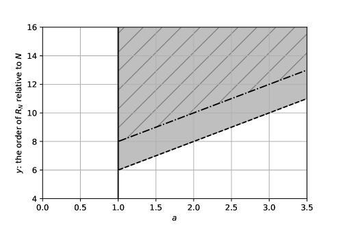
Figure 1: An illustration of Conditions 4 and 4^∗. The graph below shows the relationship between the eigenvalue decay rate $a$ ($x$-axis) and the polynomial order of truncation $R_{N}$ ($y$-axis). The outer shaded area, which is surrounded by $a>1$ (solid line) and $y>2a+4$ (dashed line), corresponds to Condition 4, while the inner shaded area (filled by dashes) surrounded by $a>1$ and $y>2a+6$ (dash-dotted line), corresponds to Condition 4^∗.

Remark.

Here we consider possibly diverging $R_{N}$ (thus $R_{N}^{*}$) to avoid missing potential signal in high-order terms, different from the tests in Aston et al. (2017); Constantinou et al. (2017); Lynch and Chen (2018) which considered finite truncation. Our proposal allows the truncation to diverge with the sample size, which is integrated into the limiting distribution and reflects the nonparametric nature of the test.

To describe the joint distribution of $T_{h}(\mathbb{I}_{R_{N}})$, of which the dimension $R_{N}^{*}$ diverges with $N$, we introduce the following Prokhorov metric $\pi$:

$$\pi(\mu,\nu)\equiv\inf\{\varepsilon\geq 0:\mu(A)\leq\nu(A^{\varepsilon})+\varepsilon\mbox{ and }\nu(A)\leq\mu(A^{\varepsilon})+\varepsilon\mbox{ for all }A\in\mathscr{B}(M)\},$$

where $(M,d_{M})$ is a metric space with its Borel sigma algebra $\mathscr{B}(M)$, $\mu$ and $\nu$ are two probability measures on the measure space $(M,\mathscr{B}(M))$, $A^{\varepsilon}=\{x:\exists y\in A,d_{M}(x,y)<\varepsilon\}$ is the $\varepsilon$-neighborhood of $A$ (e.g., Billingsley, 1999, Section 6 of Chapter 1).

Theorem 2.

Assume that the conditions of Theorem 1 and Condition 4^∗ hold, and $N_{h}\asymp N$. If $X({\boldsymbol{s}},t)$ is weakly separable, then

$$\pi\left(T_{h}(\mathbb{I}_{R_{N}}\right),{\cal Z}_{R_{N}^{*}})\longrightarrow 0,$$

where ${\cal Z}_{R_{N}^{*}}\sim N_{R_{N}^{*}}(0,\Gamma)$ is a $R_{N}^{*}$-dimensional Gaussian random vector with mean zero and covariance matrix $\Gamma$ given in (32) in Appendix C, and $\pi(\cdot,\cdot)$ is the Prokhorov metric.

To derive our test statistic for weak separability, we need to estimate $\Gamma$, which, according to the explicit expression (32) in Appendix C, relies on the cross fourth-order moments of the FPC scores, i.e., ${\rm E}(\xi_{i_{1}j}\xi_{i_{2}k}\xi_{i_{3}j^{\prime}}\xi_{i_{4}k^{\prime}})$, $(j,k),(j^{\prime},k^{\prime})\in\mathbb{I}_{R_{N}}$ and $i_{1},i_{2},i_{3},i_{4}=1,\dots,N$. Note that Condition 1 implies the boundedness of these cross fourth-order moments for a weakly separable process. While the assumed second-order stationarity for the projected spatial random fields {$\xi_{r}(\cdot)$} makes it possible to estimate the second-order moments by borrowing information spatially, additional assumptions would be needed in order to estimate these higher-order moments. In this paper, we assume that {$\xi_{r}(\cdot)$} are Gaussian. We note that Gaussian random fields have been widely studied in spatial statistics and that similar assumptions have been also made in the functional data setting (Aston et al., 2017). We also provide more discussion about the Gaussian assumption with some sensitivity analysis and numerical results in Section S.2 of the Supplementary Material.

Under the assumed Gaussionality, the projected random fields {$\xi_{r}(\cdot)$} would be jointly independent across $r$. Consequently the cross fourth moments ${\rm E}(\xi_{i_{1}j}\xi_{i_{2}k}\xi_{i_{3}j^{\prime}}\xi_{i_{4}k^{\prime}})$ become 0 for $j\not=j^{\prime}$ or $k\not=k^{\prime}$, and the off-diagonal elements $\mbox{cov}\{T_{h}(j,k),T_{h}(j^{\prime},k^{\prime})\}$ based on ${\rm E}(\xi_{i_{1}j}\xi_{i_{2}k}\xi_{i_{3}j^{\prime}}\xi_{i_{4}k^{\prime}})$ would all be 0. For the diagonal elements, the cross moments ${\rm E}(\xi_{i_{1}j}\xi_{i_{2}k}\xi_{i_{3}j}\xi_{i_{4}k})$ can also be expressed by the products of ${\rm E}(\xi_{i_{1}j}\xi_{i_{3}j})$ and ${\rm E}(\xi_{i_{2}k}\xi_{i_{4}k})$ due to independence. According to Theorem 2, the vector $T_{h}(\mathbb{I}_{R_{N}})$ can be approximated by a $R_{N}^{*}$-dimensional multivariate Gaussian distribution. We then formulate the proposed $\chi^{2}$ test statistic as

$$S_{h}(\mathbb{I}_{R_{N}})=\sum_{(j,k)\in\mathbb{I}_{R_{N}}}\{T_{h}(j,k)/\sigma_{j,k}\}^{2},$$ (24)

where {$\sigma_{j,k}^{2}$} are the diagonal elements of $\Gamma$ as in (25).

Corollary 1.

Under the conditions of Theorem 2, and the additional assumption that $X({\boldsymbol{s}},t)$ is Gaussian, the covariance matrix $\Gamma$ in Theorem 2 becomes diagnal, $\Gamma=\mbox{diag}\{\sigma^{2}_{j,k}:(j,k)\in\mathbb{I}_{R_{N}}\}$ with the elements

$$\sigma^{2}_{j,k}=\frac{1}{N}\mbox{tr}(U_{j}U_{k})+\frac{N}{(\rho_{jk}^{(h)}N_{h})^{2}}\mbox{tr}(U_{j,1}U_{k,2})-\frac{2}{\rho_{jk}^{(h)}N_{h}}\mbox{tr}(V_{j,1}V^{{}^{\rm T}}_{k,2}),$$ (25)

where $\rho_{jk}^{(h)}$ is defined in (23), $U_{r}={\rm E}(\bm{\xi}_{r}\bm{\xi}_{r}^{{}^{\rm T}})$ is the covariance matrix of $\bm{\xi}_{r}=(\xi_{1r},\dots,\xi_{Nr})^{{}^{\rm T}}$, and $U_{r,1},U_{r,2},V_{r,1},V_{r,2}$ are covariance matrices based on $U_{r}$ with explicit formulas given in (33) in Appendix C. Moreover, we have

$$\pi\left(S_{h}(\mathbb{I}_{R_{N}}),\chi^{2}_{R_{N}^{*}}\right)\longrightarrow 0,$$

where $\chi^{2}_{R_{N}^{*}}$ is a chi-squared distribution with $R_{N}^{*}=R_{N}(R_{N}-1)/2$ degrees of freedom, and $\pi(\cdot,\cdot)$ is the Prokhorov metric.

3.4 Implementation and parameter selection

According to Corollary 1, we can perform a $\chi^{2}$ test based on $S_{h}(\mathbb{I}_{R_{N}})$, with an estimate of $\Gamma$ and a suitable truncation $R_{N}$. For the choice of $R_{N}$, Conditions 4 and 4^∗ provide merely theoretical magnitudes. On the other hand, $R_{N}$ cannot be too small, so that under the alternative hypothesis the signal for $\{\xi_{r}:r\leq R_{N}\}$ can be detected. In practice, we suggest to conduct the proposed test over a range of $R_{N}$, e.g. as determined by the fraction of variance explained (FVE), $\mbox{FVE}(R_{N})=\{\sum_{r=1}^{R_{N}}\hat{\eta}_{r}^{(h)}\}/(\sum_{r=1}^{\infty}\hat{\eta}_{r}^{(h)})$ for FVE=80%, 90% or 95% etc. Here we use the eigenvalues $\{\hat{\eta}_{r}^{(h)}\}$ calculated from the empirical lag covariance $\widehat{C}^{(h)}(t_{1},t_{2})$, instead of $\{\hat{\omega}_{r}\}$ from the empirical covariance function $\widehat{C}(t_{1},t_{2})$, as the statistic $T_{h}(j,k)$ is constructed based on the lag covariance. Under the null hypothesis, according to the definition of weak separability, the test results should agree when using different values of $R_{N}$. On the other hand, when $X({\boldsymbol{s}},t)$ is not weakly separable, $\xi_{j}(\cdot)$ and $\xi_{k}(\cdot)$ are correlated for some $(j,k)$ and the corresponding $T_{h}(j,k)$ may be large. Therefore, an appropriate $R_{N}$ should include all correlated FPC fields and a reliable conclusion can be made with agreements across different $R_{N}$ values. This is demonstrated in the data applications in Section 5, and more discussion and simulation results about the choice of $R_{N}$ are given in Section S.3.1 of the Supplementary Material.

For the estimation of the covariance matrix $\Gamma$, according to (25) in Corollary 1, we need to estimate {$\rho_{jk}^{(h)}:(j,k)\in\mathbb{I}_{R_{N}}$} and the covariance matrices {$U_{r}:r=1,\dots,R_{N}$}. To estimate $\rho_{jk}^{(h)}$ defined in (23), we need to estimate two sets of eigenvalues {$\hat{\omega}_{r}$} and {$\hat{\eta}_{r}^{(h)}$} which could be obtained by eigen-decompositions of the sample covariance $\widehat{C}(t_{1},t_{2})$ and the lag covariance $\widehat{C}^{(h)}(t_{1},t_{2})$, respectively. In practice we first obtain {$\hat{\eta}_{r}^{(h)},\hat{\psi}_{r}^{(h)}$} from $\widehat{C}(h;t_{1},t_{2})$ for $r=1,2,\dots,R_{N}$ with $\hat{\eta}_{1}^{(h)}>\hat{\eta}_{2}^{(h)}>\dots\geq 0$. The corresponding {$\hat{\omega}_{r}$} can be determined by simply matching the estimated eigenfunctions of $\widehat{C}$, denoted by {$\hat{\psi}_{r^{\prime}}:r^{\prime}\geq 1$}, to {$\hat{\psi}_{r}^{(h)}:r\geq 1$} by $\hat{\psi}_{r}=\arg\max_{\psi_{r^{\prime}}}\{|\int\hat{\psi}_{r}^{(h)}(t)\hat{\psi}_{r^{\prime}}(t)dt|:r^{\prime}\geq 1\}$, which performs well in our numerical studies. We then estimate $\rho_{jk}^{(h)}$ by $\hat{\rho}_{jk}^{(h)}=({\hat{\eta}_{j}^{(h)}-\hat{\eta}_{k}^{(h)}})/({\hat{\omega}_{j}-\widehat{\omega}_{k}})$ for each $(j,k)$.

For the estimation of covariance matrices {$U_{r}:r=1,\dots,R_{N}$}, we first note that the diagonal elements in $U_{r}$ are the variance of $\xi_{r}(\cdot)$, thus can be estimated by $\hat{\omega}_{r}$. To estimate the off-diagonal elements in $U_{r}$, i.e. the cross-covariance ${\rm E}\{\xi_{r}({\boldsymbol{s}}_{i})\xi_{r}({\boldsymbol{s}}_{i^{\prime}})\}$ when ${\boldsymbol{s}}_{i}\not={\boldsymbol{s}}_{i^{\prime}}$, note that under the spatial stationarity we can derive

$${\rm E}\{\xi_{r}({\boldsymbol{s}}_{i})\xi_{r}({\boldsymbol{s}}_{i^{\prime}})\}=\omega_{r}\rho_{r}(|{\boldsymbol{s}}_{i}-{\boldsymbol{s}}_{i^{\prime}}|),$$ (26)

where $\rho_{r}(\cdot)$ is a correlation function that could vary with $r$. For each pairwise distance $d$ in the set ${\cal D}=\{|{\boldsymbol{s}}_{i}-{\boldsymbol{s}}_{i^{\prime}}|:{\boldsymbol{s}}_{i}\not={\boldsymbol{s}}_{i^{\prime}},{\boldsymbol{s}}_{i}\in{\cal S},{\boldsymbol{s}}_{i^{\prime}}\in{\cal S}\}$, we estimate $\rho_{r}(d)$ by $\tilde{\rho}_{r}(d)=({N_{d}}^{-1}\sum_{|{\boldsymbol{s}}_{i}-{\boldsymbol{s}}_{i^{\prime}}|=d}\hat{\xi}_{ir}\hat{\xi}_{i^{\prime}r})/\hat{\omega}_{r}$, where $N_{d}$ is the total number of pairs (${\boldsymbol{s}}_{i},{\boldsymbol{s}}_{i^{\prime}}$) separated by a distance $d$. Then we could use either parametric or non-parametric methods to estimate $\rho_{r}(\cdot)$ based on {$\tilde{\rho}_{r}(d):d\in{\cal D}$}. Many classical parametric models in spatial statistics (Cressie and Wikle, 2015) can be used. Taking as an example, we perform a weighted least square approach (Sherman, 2011) on {$\tilde{\rho}_{r}(d):d\in{\cal D}$} to fit an exponential model $\exp(-|{\boldsymbol{s}}_{i}-{\boldsymbol{s}}_{j}|/\phi)$ with the scale parameter $\phi$. Then $\rho_{r}(d)$ is estimated by $\exp(-d/\hat{\phi}_{r})$ with the weighted least square estimator $\hat{\phi}_{r}$ for each $r$. Alternatively, a smooth estimate of $\rho_{r}(\cdot)$ could also be obtained by a nonparametric regression approach, such as a local linear estimation (Fan and Gijbels, 1996) on {$d,\tilde{\rho}_{r}(d):d\in{\cal D}$}. We evaluate the performance of parametric and non-parametric methods via simulation studies in Section 4.

An important issue is the choice of the spatial lag $h$. For spatial data, it is common that observations separated by smaller lags are more correlated. Evidence for any departure from weak separability is usually stronger when the test statistic is formed by using a smaller $h$, at least as compared to using a much larger lag at which the correlation may be negligible. For data observed on a regular space ${\cal S}\subset\mathbb{Z}^{2}$, where $\mathbb{Z}^{2}$ can be regarded as the two-dimensional space of the integer lattice points with minimum grid distance, saying $d_{0}=1$, we could naturally use a lag-$z$ covariance estimator where $z$ is a positive integer such that $h=zd_{0}$. Our simulation results in Section 4 provide empirical support for using small lags, which also coincides with the theoretical consideration of small neighborhood of $h$.

Remark.

We also consider combining information from a range of $h$ using multiple tests, and provide the relevant results based on the Bonferroni correction in Section S.3.2 of the Supplementary Material. It is seen that this testing procedure combining different lags has reasonable size, but is less powerful than the test using lag-1 covariance. This is expected given that our simulation results in Section 4 also indicate that the test using lag-1 covariance is the most powerful.

4 Simulation Study

In this section we assess the performance of the proposed test. Set the time domain $T=[0,1]$ with 100 equally spaced time points, and the spatial region be a regular grid on $D=[0,2]\times[0,2]$ whose spatial grid increment is $0.05$, i.e., the number of spatial points $N=40^{2}=1600$. We generate $X({\boldsymbol{s}},t)$ from the model, $X({\boldsymbol{s}},t)=\mu(t)+\sum_{r=1}^{p}\xi_{r}({\boldsymbol{s}})\psi_{r}(t)$, using a mean function $\mu(t)=3+2t^{2}$ as in Li and Guan (2014), and $p=10$ basis functions, $\psi_{r}(t)=\sqrt{2}\cos(r\pi t)$ when $r$ is odd and $\psi_{r}(t)=\sqrt{2}\sin\{(r-1)\pi t\}$ when $r$ is even as in Kong et al. (2016). The {$\xi_{r}(\cdot)$} are generated marginally from Gaussian random fields, with isotropic Matérn covariance structures $c_{r}({\boldsymbol{s}}_{1}-{\boldsymbol{s}}_{2};\nu,\phi)=\omega_{r}\mbox{M}(|{\boldsymbol{s}}_{1}-{\boldsymbol{s}}_{2}|;\nu,\phi)$ with $\omega_{r}=4r^{-2}$ and

$$\mbox{M}(d;\nu,\phi)=\frac{2^{1-\nu}}{\Gamma(\nu)}(\frac{d}{\phi})^{\nu}K_{\nu}(\frac{d}{\phi}).$$

In the above, $K_{\nu}$ is the modified Bessel function of the second type of order $\nu$, where $\nu$ controls the smoothness of the process, and $\phi>0$ is the range parameter controlling the rate of decay of spatial correlation, where a larger $\phi$ corresponds to a stronger correlation (Cressie and Wikle, 2015). We set $(\phi_{1},\phi_{2},\phi_{3},\phi_{4})=(0.2,0.1,0.15,0.08)$, and $\phi_{5},\dots,\phi_{10}=0$ (i.e., no spatial correlation) for the high-order principal components.

To study the power, we generate $\{\xi_{1}(\cdot),\xi_{2}(\cdot)\}$ from a bivariate Matérn model (Gneiting et al., 2010) using the above marginal covariance functions:

$$c_{1}(d)=\omega_{1}\mbox{M}(d;\nu_{1}=1,\phi_{1}=0.2),\quad c_{2}(d)=\omega_{2}\mbox{M}(d;\nu_{2}=0.5,\phi_{2}=0.1),$$

and the following cross-covariance function:

$$c_{12}(d)=\rho_{12}\sqrt{\omega_{1}\omega_{2}}\mbox{M}(d;\nu_{12}=0.8,\phi_{12}=0.15).$$

Here the coefficient $\rho_{12}=0$ yields the null hypothesis, i.e., the spatial random fields $\xi_{r}(\cdot)$ are mutually uncorrelated. The correlation between $\xi_{1}(\cdot)$ and $\xi_{2}(\cdot)$ increases as $\rho_{12}$ becomes larger, facilitating the departure from weak separability. The setup of $(\nu_{1},\nu_{2},\nu_{12})$ satisfies the condition in Theorem 3 of Gneiting et al. (2010), such that the above bivariate Matérn model is valid. The other {$\nu_{r}$} are all set to be $0.5$ for $3\leq r\leq 10$, noting that $\mbox{M}(d;\nu=0.5,\phi)$ reduces to the exponential model.

We implement the parametric and nonparametric methods in Section 3.4 based on the empirical lag covariance with the 0.05 significance level. The empirical size and power are assessed with 1000 Monte Carlo runs. We investigate the test performance using different FVE threshold values (80%, 90% or 95%), shown in Table 1 the empirical rejection rate results using the lag-$z$ covariance defined in Section 3.4 from $z=1$ to 4. We can see that when $\rho_{12}=0$, both the parametric and non-parametric tests have reasonable sizes across different lag choices, and the rejection rates rise rapidly for all the methods as $\rho_{12}$ grows from 0.2 to 0.6. It is clear that the lag-1 covariance is the most powerful and the test performance deteriorates substantially as the lag increases, especially when $\rho_{12}=0.4$ or 0.6. This supports the advantage of using small lags, as discussed in Section 3.4, in order to detect departures from weak separability. Therefore, in practice we suggest to focus more on the test results based on the lag-1 covariance estimation for data collected on a regular spatial grid.

Table 1: Rejection rates (%) for the weak separability tests based on the lag covariance under different FVEs, with the asymptotic covariance estimated by parametric (Para) and non-parametric (Nonp) methods.

		lag-1			lag-2			lag-3			lag-4
$\rho_{12}$	FVE	Para	Nonp		Para	Nonp		Para	Nonp		Para	Nonp
0	80%	4.2	3.4		6.4	4.2		7.4	5.3		6.6	5.4
	90%	4.7	5.4		6.4	4.2		7.3	5.2		6.5	5.3
	95%	5.6	6.9		7.9	8.3		6.6	6.5		6.1	5.2
0.2	80%	85.0	87.5		76.5	69.5		33.0	32.5		12.0	15.5
	90%	74.5	79.5		74.0	67.5		32.0	32.0		12.0	15.5
	95%	70.5	77.5		63.5	62.5		27.5	31.5		12.0	15.5
0.4	80%	100	100		94.0	94.0		68.0	69.0		32.5	37.0
	90%	95.0	94.5		95.0	94.5		68.5	69.5		32.5	37.5
	95%	100	100		98.5	98.0		73.5	77.0		31.0	39.0
0.6	80%	100	88.0		89.0	82.0		67.5	68.0		37.0	41.0
	90%	100	100		90.0	91.0		68.0	68.0		37.0	41.0
	95%	100	100		99.5	99.5		79.5	81.5		41.5	47.5

Note that, for the lag-1 covariance, $R_{N}$ is selected to be 2 in nearly all 1000 trials when the FVE is set to 80%. When FVE$\,=\,$90%, the proportions of instances in which $R_{N}=2$ and $R_{N}=3$ are 33% and 66%, respectively, and when FVE$\,=\,$95% the proportion is 91% for $R_{N}=3$ and 9% for $R_{N}=4$. As explained in Section 3.4, the proposed test is usually stable under the null hypothesis for different $R_{N}$ values, though the size may be inflated for overly large $R_{N}$. On the other hand, the results under alternative depends on the occurrence of non-separable components. In our settings, the correlation emerges for the first two FPC scores, thus the power seems to be better if $R_{N}=2$ is mostly selected, i.e., FVE=80%, which is seen in Table 1. As expected, the power increases as $\rho_{12}$ grows that makes the first two components more non-separable. As a practical guidance, the claim of weak separability should be a comprehensive conclusion across different $R_{N}$ or FVE values. More discussion and simulation regarding the choice of $R_{N}$ are given in Section S.3.1 of the Supplementary Material. Lastly we see that the results based on parametric and nonparametric modeling of correlation are very similar. We also perform the tests with different range parameters (see Section S.4 of the Supplementary Material) and different space/time window (not reported for space concerns), and both studies yield similar results.

5 Real Data Application

5.1 China PM_2.5 data

Chronic and severe air pollution has affected a significant portion of China in recent years. Among all air pollutants, the fine particulate matter with aerodynamic diameters less than 2.5 $\mu m$, also known as PM_2.5, is considered to have the most damaging effect on health. It is a common practice to analyze time-varying environmental variables using functional data analysis, see examples of temperature and log-precipitation curves in Ramsay and Silverman (2005) and wind speed data in Constantinou et al. (2017). Recent research on statistical modeling of China PM_2.5 has also received considerable attention, see Liang et al. (2015) and Zhang et al. (2017).

The Chinese government started monitoring PM_2.5 concentrations from 2013 and have established a large national monitoring network for air quality assessment by 2017. Real-time measurements of major pollutants across nearly 1,500 monitoring sites in 369 cities are continuously recorded and sent to the China National Environmental Monitoring Center (CNEMC) (Zhang et al., 2017; Wu et al., 2018). The PM_2.5 data used in our analysis are constructed based on the Nested Air Quality Prediction Modeling System (NAQPMS), which is a multi-scale chemical transport model proposed by the Institute of Atmospheric Physics, Chinese Academy of Sciences (Wang et al., 2006). The NAQPMS simulates the chemical and physical processes of air pollutants by solving the mass balance equation using terrain-following vertical coordinates. The output PM_2.5 concentrations cover the entire China and have a $15$ km $\times$ $15$ km horizontal resolution on a regular $432\times 339$ spatial grid.

China has a topologically diverse landscape, and the entire spatial region may be too large to impose stationarity, we choose 6 subregions according to the topographic division of China: the North China Plain (NCP), Yangtze River Delta (YRD), Pearl River Delta (PRD), Sichuan Basin (SB), Xinjiang (XJ) and Tibet (TB). Figure 2 displays an overview of these regions. In each region we extract a $40\times 40$ grid from the whole dataset for ease of computation, with hourly recordings from December 1 to 30, 2016. Based on averaging every 4 consecutive hours, the number of time points is $30$ (days) $\times$ $6=180$. To check the spatial stationarity we perform a sensitivity analysis, and the results (provided in the Section S.1 of the Supplementary Material) suggest that there is no serious violation.

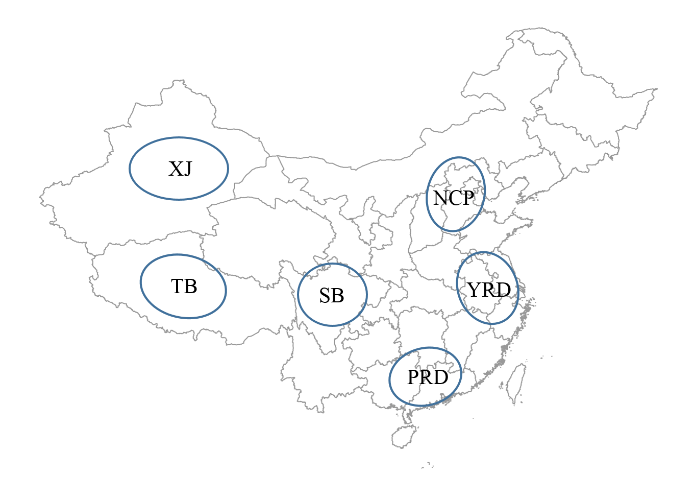
Figure 2: Locations of the 6 subregions in the weak separability tests for China PM_2.5 data.

We apply the proposed test in the above 6 regions based on the lag-1 covariance due to its advantage from methodological and empirical perspectives, with truncation of 80%, 90% and 95% FVEs respectively. The resulting $p$-values are summarized in Table 2. We can see that the results of the parametric and nonparametric methods using different FVEs are in agreement: the hypothesis of weak separability is rejected for XJ and TB but not for the other 4 regions. This is an interesting phenomenon because the four non-rejected regions are relatively more developed areas in China. It has been reported that the formation and transmission mechanism of PM_2.5 exhibits completely different patterns in XJ and TB located mainly in the deserts and plateaus of western China (Wang et al., 2015). Based on our analysis, it is reasonable to assume weak separability for modeling the PM_2.5 data in east-central China, but not in XJ or TB regions.

Table 2: The $p$-values of weak separability tests using parametric (Para) and nonparametric (Nonp) methods with different truncation levels for China PM_2.5 data.

Region	NCP	YRD	PRD	SB	XJ	TB
FVE = 80%	$R_{N}=2$	$R_{N}=3$	$R_{N}=2$	$R_{N}=3$	$R_{N}=2$	$R_{N}=3$
Para	0.136	0.925	0.722	0.937	0.002	0.000
Nonp	0.287	0.620	0.709	0.663	0.000	0.000
FVE = 90%	$R_{N}=3$	$R_{N}=6$	$R_{N}=3$	$R_{N}=6$	$R_{N}=5$	$R_{N}=5$
Para	0.150	0.863	0.713	0.535	0.000	0.000
Nonp	0.212	0.399	0.690	0.440	0.000	0.000
FVE = 95%	${R_{N}=6}$	$R_{N}=9$	$R_{N}=6$	$R_{N}=9$	$R_{N}=8$	$R_{N}=8$
Para	0.759	0.997	0.521	0.366	0.000	0.000
Nonp	0.289	0.119	0.230	0.117	0.000	0.000

5.2 Harvard Forest data

This dataset consists of the Enhanced Vegetation Index (EVI) series at Harvard Forest, which were previously studied by Liu et al. (2017). The EVI is calculated from surface spectral reflectance measurements collected from moderate-resolution imaging spectroradiometers onboard NASA’s Terra and Aqua satellites. Specifically, the data are extracted for a 25 by 25 pixel window (covering an area of approximately 134 km²), centered over the Harvard Forest Long Term Experimental Research site in Petershan, MA. The EVI data are recorded from 2001 to 2006 at 8-day intervals, see Liu et al. (2017) for more details. By averaging 3 consecutive temporal observations to reduce noise, the dataset used in our analysis has 625 spatial grids and 92 time points.

Liu et al. (2017) proposed a spatial PACE model based on Yao et al. (2005) to reconstruct the spatial functional data and perform an isotropy test. According to the study of Liu et al. (2017), it is reasonable to assume spatial stationarity, which is also verified by our sensitivity analysis similar to that used for the China’s PM_2.5 data example. We notice that weak separability is assumed in their spatial functional model and forms a foundation for subsequent analysis. We now examine the appropriateness of weak separability, and apply the proposed test based on the lag-1 covariance. The results show that the FVEs for the first two and three components are respectively 69.8% and 78.5%. The corresponding $p$-values using the parametric and nonparametric methods are 0.872 and 0.880, respectively, when $R_{N}$ is 2, and are 0.073 and 0.079 when $R_{N}$ is 3. Interestingly, as $R_{N}$ increases to 4 (corresponding to FVE=84.1%), the $p$-values become 0.018 and 0.019, then they decrease to less than 0.01 when more than 5 components are considered. This indicates that the correlated FPC fields that violate the weak separability assumption do not emerge until $R_{N}=4$. Our results suggest that, if considering a rough representation with no more than 3 components explaining around 80% FVE, the model used in Liu et al. (2017) which focuses primarily on the first two FPCs seems reasonable. However, if we are interested in a comprehensive spatio-temporal functional data model that contains more components, the weak separability assumption appears not valid.

6 Discussion and Conclusion

In this work we introduce a sensible definition of weak separability for spatial functional field. This flexible yet parsimonious representation views the space and time domains from different perspectives with ease of modeling/computation and interpretation. By means of the lag covariance function, we develop a formal hypothesis test based on the asymptotic distribution that is easy to handle under Gaussian assumption and does not require computationally intensive resampling procedures, such as bootstrap approximations. In particular, our methods are motivated by (and more applicable to) the typical non-replicated spatio-temporal data. We implemented the test procedures for the Harvard Forest data and China PM_2.5 data, and obtained interesting and insightful results. We recommend to exploit the proposed test prior to further statistical analysis that often imposes weak separability assumption for feasible modeling.

For future work, the proposed procedure deals with data observed on a dense temporal grid, which can be extended to the case of sparse functional observations with measurement errors (Yao et al., 2005; Liu et al., 2017) through an adaptation of lag covariance estimation. For instance, if the data are spatially irregularly spaced, one could implement the kernel smoothing methods mentioned in Section 2.2 with more involved technical development. For those whose data show obvious spatial anisotropy, the lag covariance in some specific directional lag can be used. Methods for testing for isotropy, such as those in Guan et al. (2004) and Liu et al. (2017), may also be studied in current context. The discussion and results in Section S.2 of the Supplementary Material provide some evidence for the sensitivity of our methods to the Gaussian assumption, and demonstrate the favorable performance of our method over other numerical methods such as the block bootstrap. However, more studies about the approximating method on the asymptotic covariance without the Gaussian assumption are still called for and exhibit challenges for the non-replicated spatio-temporal data. Another potential topic is spatio-temporal point process, where the spatial functional process act as a latent effect and is related to the intensity function of the point process with a nonlinear link function (Li and Guan, 2014).

Supplementary Material

For space economy, we collect more discussions and additional results on spatial stationarity and Gaussian assumption, some implementation issues for the choices of truncation parameter and spatial lag, and some technical proofs of the propositions and lemmas in an online Supplementary Material.

Appendix Appendix A Notation

We first introduce some notations in Hilbert spaces. Let ${\cal H}$ be a real separable Hilbert space with the usual inner product $\left<f,g\right>=\int f(t)g(t)dt$. As standard definitions in Aston et al. (2017) the space of Hilbert-Schmidt operators on ${\cal H}$ is denoted as ${\cal B}_{HS}({\cal H})$, and is a Hilbert space with the inner product $\left<K_{1},K_{2}\right>_{HS}=\sum_{i\geq 1}\left<K_{1}(e_{i}),K_{2}(e_{i})\right>$ and the induced norm $\|\cdot\|_{HS}$. For $z,y\in{\cal H}$, $z\otimes y$ is the operator defined by $(z\otimes y)(x)=\left<z,x\right>y$, and so for $z,y\in{\cal B}_{HS}({\cal H})$. A spatial functional field $X({\boldsymbol{s}},t)$ at fixed ${\boldsymbol{s}}$ is denoted as $X({\boldsymbol{s}})\in L^{2}({\cal T})$ with the mean function $\mu({\boldsymbol{s}})={\rm E}X({\boldsymbol{s}})$. The covariance operator of $X({\boldsymbol{s}})$ is defined by ${\bm{C}}_{{\boldsymbol{s}},{\boldsymbol{s}}}={\rm E}\left[\left\{X({\boldsymbol{s}})-\mu({\boldsymbol{s}})\right\}\otimes\left\{X({\boldsymbol{s}})-\mu({\boldsymbol{s}})\right\}\right]$, and the cross covariance operator at fix locations ${\boldsymbol{s}}_{1}$ and ${\boldsymbol{s}}_{2}$ is defined as ${\bm{C}}_{{\boldsymbol{s}}_{1},{\boldsymbol{s}}_{2}}={\rm E}\left[\left\{X({\boldsymbol{s}}_{1})-\mu({\boldsymbol{s}}_{1})\right\}\otimes\left\{X({\boldsymbol{s}}_{2})-\mu({\boldsymbol{s}}_{2})\right\}\right]$ (Hsing and Eubank, 2015; Hörmann and Kokoszka, 2011). For a spatially stationary functional field $X({\boldsymbol{s}},t)$ with the mean function as $\mu=\mu({\boldsymbol{s}})$, the covariance estimator

$${\bm{C}}={\rm E}\left[\left\{X({\boldsymbol{s}})-\mu\right\}\otimes\left\{X({\boldsymbol{s}})-\mu\right\}\right],$$

and the lag covariance operator ${\bm{C}}^{(h)}$ is defined by

$${\bm{C}}^{(h)}={\rm E}\left[\left\{X({\boldsymbol{s}}_{1})-\mu\right\}\otimes\left\{X({\boldsymbol{s}}_{2})-\mu\right\}\right],\mbox{ where }|{\boldsymbol{s}}_{1}-{\boldsymbol{s}}_{2}|=h,$$

under isotropy. The covariance function $C(t_{1},t_{2})$ and $C^{(h)}(t_{1},t_{2})$ defined in Section 2.2 can be seen as the kernel of the operator ${\bm{C}}$ and ${\bm{C}}^{(h)}$; see Chapter 7.2 and 7.3 of Hsing and Eubank (2015) for more details about the (cross) covariance operators in Hilbert space. Assume we observe $\{X({\boldsymbol{s}}_{i})\}_{i=1,\dots,N}$ from $X({\boldsymbol{s}})$, and denote $X_{i}=X({\boldsymbol{s}}_{i})$. We estimate $\mu$ by the sample mean $\bar{X}=N^{-1}\sum_{i=1}^{N}X_{i}$, and ${\bm{C}}$ by the sample covariance operator

$$\widehat{\bm{C}}=\frac{1}{N}\sum_{i=1}^{N}(X_{i}-\bar{X})\otimes(X_{i}-\bar{X}).$$ (27)

Let $\mathscr{A}_{h}=\{(i,i^{\prime}):|{\boldsymbol{s}}_{i}-{\boldsymbol{s}}_{i^{\prime}}|=h\}$ be the set of location pairs at lag $h$, and $N_{h}=|\mathscr{A}_{h}|$ be the cardinality of $\mathscr{A}_{h}$. We then have the empirical lag covariance operator given by

$$\widehat{\bm{C}}^{(h)}=\frac{1}{N_{h}}\sum_{(i,{i^{\prime}})\in\mathscr{A}_{h}}(X_{i}-\bar{X})\otimes(X_{i^{\prime}}-\bar{X}).$$

It can be seen that all these operators ${\bm{C}}$, ${\bm{C}}^{(h)}$, $\widehat{\bm{C}}$ and $\widehat{\bm{C}}^{(h)}$ belong to ${\cal B}_{HS}\{L^{2}({\cal T})\}$ (Hsing and Eubank, 2015). To be more concise and without confusion, in what follows we denote $\psi(t)$ as $\psi$, $\hat{\psi}_{r}^{(h)}(t)$ as $\hat{\psi}_{r}^{(h)}$, $\int C(t_{1},t_{2})\psi(t_{1})dt_{1}$ as $\int{\bm{C}}\psi$, and $\iint C(t_{1},t_{2})\psi_{j}(t_{1})\psi_{k}(t_{2})dt_{1}dt_{2}$ as $\int{\bm{C}}\psi_{j}\psi_{k}$.

Appendix Appendix B Proof of Theorem 1

We first state some technical lemmas for the main theorems. Lemmas 1 and 2 provide the asymptotic results for the covariance and lag covariance estimators. Lemma 3 provides the perturbation results for the estimates obtained by FPCA, which serve as building blocks for establishing the moment bound result in Theorem 1.

Lemma 1.

Consider the covariance operator $\widehat{\bm{C}}$ defined in (27) with $X_{i}\overset{\text{i.i.d}}{\sim}X\in L^{2}({\cal T})$. If ${\rm E}\|X_{i}\|^{4}<\infty$, then $N^{1/2}(\widehat{\bm{C}}-{\bm{C}})$ converges in distribution to a mean-zero Gaussian random element in ${\cal B}_{HS}\{L^{2}({\cal T})\}$.

Remark.

Here ${\rm E}\|X_{i}\|^{4}<\infty$ is a sufficient condition for the CLT of covariance operators under the Hilbert-Schmidt topology. This is a weaker assumption than Condition 2.1 in Aston et al. (2017) that $\sum_{r=1}^{\infty}({\rm E}([\left<X,e_{r}\right>^{4}])^{1/4}<\infty$ for some orthonormal basis $(e_{r})_{r\geq 1}$, which is required to prove the weak convergence under the trace-norm topology (see Remark 3.2 of Bagchi et al., 2020).

Lemma 2.

Consider a spatially stationary functional field $X({\boldsymbol{s}})\in L^{2}({\cal T})$ with covariance and lag covariance operators defined in Appendix A. Under Conditions 1 and 2, $[N^{1/2}(\widehat{\bm{C}}-{\bm{C}}),N_{h}^{1/2}\{\widehat{\bm{C}}^{(h)}-{\bm{C}}^{(h)}\}]$ converges in distribution to a mean-zero Gaussian random element in ${\cal B}_{HS}\{L^{2}({\cal T})\}\times{\cal B}_{HS}\{L^{2}({\cal T})\}$.

Define the set of realizations such that, for sample size $N$, some C and any $\tau<1$,

$${\cal E}_{N,R_{N}}=\left\{\left(\hat{\eta}_{j}^{(h)}-\eta_{k}^{(h)}\right)^{-2}\leq 2\left(\eta_{j}^{(h)}-\eta_{k}^{(h)}\right)^{-2}\leq CN^{\tau},j,k=1,\dots,R_{N},j\not=k\right\}.$$ (28)

Lemma 3.

(a) Under Conditions 1 to 4, we have ${\mathbb{P}}({\cal E}_{N,R_{N}})\rightarrow 1$ as $N\rightarrow\infty$.
(b) Under Conditions 1 to 4, for each integer $b>0$, on the high probability set ${\cal E}_{N,R_{N}}$,

$${\rm E}\|\hat{\psi}_{j}^{(h)}-\psi_{j}\|^{2b}=O\{(j^{2}N^{-1})^{b}\},$$

and $O(\cdot)$ is uniform in $j=1,\dots,R_{N}$.
(c) Under Conditions 1 to 4, on the high probability set ${\cal E}_{N,R_{N}}$,

$$\hat{\psi}_{j}^{(h)}(t)-\psi_{j}(t)=\sum_{k:k\not=j}(\eta_{j}^{(h)}-\eta_{k}^{(h)})^{-1}\psi_{k}(t)\int\left(\widehat{\bm{C}}^{(h)}-{\bm{C}}^{(h)}\right)\psi_{j}\psi_{k}+\alpha_{j}(t),$$ (29)

where

$${\rm E}\|\alpha_{j}\|^{2}=O(j^{2a+4}N^{-2})$$

uniformly in $j=1,\dots,R_{N}$.

Remark.

The moment bound for $\|\hat{\psi}_{j}^{(h)}-\psi_{j}\|^{2b}$ with diverging truncation provides a stronger result than the consistency of $\hat{\psi}_{j}^{(h)}$, i.e., $O_{p}(\cdot)$ type. The expansion (29) follows directly from Lemma 1 of Kong et al. (2016) or (5.22) of Hall and Hosseini-Nasab (2009). It has been shown that $\|\alpha_{j}\|=O_{p}(j^{a+2}N^{-1})$ in Kong et al. (2016). However, to derive the convergence rate for $\|T_{h}(\mathbb{I}_{R_{N}})-T_{h}^{*}(\mathbb{I}_{R_{N}})\|^{2}$ in Theorem 2, which is based on a sum over a diverging truncation set of indices for the error terms, we need the moment bounds for $\|\alpha_{j}\|^{2}$ over this truncation set. The proof of Lemma 3 is based on similar arguments and moment calculations in Kong et al. (2016) and Hall and Hosseini-Nasab (2009); see Section S.5.2 of the Supplementary Material.

Proof of Theorem 1.

Using the notations in Appendix A, we denote the eigen-decomposition in (12) as $\int\widehat{\bm{C}}^{(h)}\hat{\psi}_{r}^{(h)}=\hat{\eta}_{r}^{(h)}\hat{\psi}_{r}^{(h)}$, and similarly $\int{\bm{C}}^{(h)}\psi_{r}=\eta_{r}^{(h)}\psi_{r}$. Recall that $\hat{\xi}_{ir}^{(h)}=\int(X_{i}-\bar{X})\hat{\psi}_{r}^{(h)}$, $i=1,\dots,N$. Then $T_{h}(j,k)$ can be expressed by

$$\frac{1}{\sqrt{N}}\sum_{i=1}^{N}\hat{\xi}^{(h)}_{ij}\hat{\xi}^{(h)}_{ik} =\frac{1}{\sqrt{N}}\iint\sum_{i=1}^{N}\left\{X_{i}(t_{1})-\bar{X}(t_{1})\right\}\hat{\psi}_{j}^{(h)}(t_{1})\left\{X_{i}(t_{2})-\bar{X}(t_{2})\right\}\hat{\psi}_{k}^{(h)}(t_{2})dt_{1}dt_{2}$$

$$=\sqrt{N}\int\widehat{\bm{C}}\hat{\psi}_{j}^{(h)}\hat{\psi}_{k}^{(h)}=\sqrt{N}\int(\widehat{\bm{C}}-{\bm{C}})\hat{\psi}_{j}^{(h)}\hat{\psi}_{k}^{(h)}+\sqrt{N}\int{\bm{C}}\hat{\psi}_{j}^{(h)}\hat{\psi}_{k}^{(h)}.$$

We shall show that both of the above two terms converge, and the leading terms are respectively $\sqrt{N}\int(\widehat{\bm{C}}-{\bm{C}})\psi_{j}\psi_{k}$ and $-{\sqrt{N}}/{\rho_{jk}^{(h)}}\int(\widehat{{\bm{C}}}^{(h)}-{\bm{C}}^{(h)})\psi_{j}\psi_{k}$. First, let $\Delta_{1}(j,k):=\sqrt{N}\int(\widehat{\bm{C}}-{\bm{C}})\hat{\psi}_{j}^{(h)}\hat{\psi}_{k}^{(h)}-\sqrt{N}\int(\widehat{\bm{C}}-{\bm{C}})\psi_{j}\psi_{k}$, then $\Delta_{1}(j,k)=\sqrt{N}\int(\widehat{\bm{C}}-{\bm{C}})(\hat{\psi}_{j}^{(h)}-\psi_{j})\hat{\psi}_{k}^{(h)}+\sqrt{N}\int(\widehat{\bm{C}}-{\bm{C}})(\hat{\psi}_{k}^{(h)}-\psi_{k})\psi_{j}$. As $\|\psi_{j}\|=\|\hat{\psi}_{k}^{(h)}\|=1$, we have $|\Delta_{1}(j,k)|\leq\sqrt{N}\,\|\widehat{\bm{C}}-{\bm{C}}\|_{HS}\,\|\hat{\psi}_{j}^{(h)}-\psi_{j}\|+\sqrt{N}\,\|\widehat{\bm{C}}-{\bm{C}}\|_{HS}\,\|\hat{\psi}_{k}^{(h)}-\psi_{k}\|\leq\sqrt{N}\,\|\widehat{\bm{C}}-{\bm{C}}\|_{HS}\,(\|\hat{\psi}_{j}^{(h)}-\psi_{j}\|+\|\hat{\psi}_{k}^{(h)}-\psi_{k}\|)$. It then follows by Cauchy-Schwarz inequality that $({\rm E}|\Delta_{1}(j,k)|)^{2}\leq C_{1}N\,{\rm E}\|\widehat{\bm{C}}-{\bm{C}}\|_{HS}^{2}\,({\rm E}\|\hat{\psi}_{j}^{(h)}-\psi_{j}\|^{2}+{\rm E}\|\hat{\psi}_{k}^{(h)}-\psi_{k}\|^{2})$, and ${\rm E}|\Delta_{1}(j,k)|^{2}\leq C_{2}N\{{\rm E}\|\widehat{\bm{C}}-{\bm{C}}\|_{HS}^{4}\,({\rm E}\|\hat{\psi}_{j}^{(h)}-\psi_{j}\|^{4}+{\rm E}\|\hat{\psi}_{k}^{(h)}-\psi_{k}\|^{4})\}^{1/2}$ for some constants $C_{1}$ and $C_{2}$. Note that ${\rm E}\|\hat{\psi}_{j}^{(h)}-\psi_{j}\|^{4}=O(j^{4}N^{-2})$ uniformly in $j=1,\dots,R_{N}$ by Lemma 3(b) with $b=2$, and ${\rm E}\|\widehat{\bm{C}}-{\bm{C}}\|_{HS}^{4}=O(N^{-2})$ according to the proof of Lemma 3(a). It then follows that ${\rm E}|\Delta_{1}(j,k)|^{2}=O(R_{N}^{2}N^{-1})$ uniformly in $j,k=1,\dots,R_{N}$ and $j\not=k$.

Next we will show the moment bound for $\Delta_{2}(j,k)=\sqrt{N}\int{\bm{C}}\hat{\psi}_{j}^{(h)}\hat{\psi}_{k}^{(h)}+{\sqrt{N}}/{\rho_{jk}^{(h)}}\int(\widehat{{\bm{C}}}^{(h)}-{\bm{C}}^{(h)})\psi_{j}\psi_{k}$. Denote $\bm{M}_{k,j}=(\eta_{j}^{(h)}-\eta_{k}^{(h)})^{-1}\int(\widehat{\bm{C}}^{(h)}-{\bm{C}}^{(h)})\psi_{j}\psi_{k}$, the equation (29) translates into $\hat{\psi}_{j}^{(h)}(t)-\psi_{j}(t)=\sum_{k:k\not=j}\bm{M}_{k,j}\psi_{k}(t)+\alpha_{j}(t)$. Then we have

$$\sqrt{N}\int{\bm{C}}\hat{\psi}_{j}^{(h)}\hat{\psi}_{k}^{(h)}=\sqrt{N}\int{\bm{C}}\left(\psi_{j}+\sum_{r:r\not=j}\bm{M}_{r,j}\psi_{r}+\alpha_{j}\right)\left(\psi_{k}+\sum_{r:r\not=k}\bm{M}_{r,k}\psi_{r}+\alpha_{k}\right).$$

Note that $\int{\bm{C}}\psi_{j}\psi_{k}=0$ for $j\not=k$ and $\int{\bm{C}}\psi_{j}\psi_{j}=\omega_{j}$, it follows that

$$\sqrt{N}\int{\bm{C}}\hat{\psi}_{j}^{(h)}\hat{\psi}_{k}^{(h)} =\sqrt{N}\int{\bm{C}}\psi_{j}(\bm{M}_{j,k}\psi_{j})+\sqrt{N}\int{\bm{C}}\psi_{k}\left(\bm{M}_{k,j}\psi_{k}\right)+\beta_{jk}$$

$$=\sqrt{N}\omega_{j}\bm{M}_{j,k}+\sqrt{N}\omega_{k}\bm{M}_{k,j}+\beta_{jk}$$

$$=\sqrt{N}(\omega_{j}-\omega_{k})\bm{M}_{j,k}+\beta_{jk}$$

$$=\sqrt{N}(\omega_{j}-\omega_{k})(\eta_{k}^{(h)}-\eta_{j}^{(h)})^{-1}\int\left(\widehat{\bm{C}}^{(h)}-{\bm{C}}^{(h)}\right)\psi_{j}\psi_{k}+\beta_{jk}.$$

Here we denote $\beta_{jk}=\beta_{1}+\beta_{2}+\beta_{3}$, where $\beta_{1}=\sqrt{N}\int{\bm{C}}\hat{\psi}_{j}^{(h)}\alpha_{k}$, $\beta_{2}=\sqrt{N}\int{\bm{C}}(\sum_{r:r\not=j}\bm{M}_{r,j}\psi_{r}+\alpha_{j})(\sum_{r:r\not=k}\bm{M}_{r,k}\psi_{r})$ and $\beta_{3}=\sqrt{N}\int{\bm{C}}\alpha_{j}\psi_{k}$. Note that $|\beta_{1}|^{2}\leq N\|C\|_{HS}^{2}\|\hat{\psi}_{j}^{(h)}\|^{2}\|\alpha_{k}\|^{2}$ and $\|\hat{\psi}_{j}^{(h)}\|=1$, it follows that ${\rm E}|\beta_{1}|^{2}\leq N|C\|_{HS}^{2}{\rm E}\|\alpha_{k}\|^{2}=O(k^{2a+4}N^{-1})$ by Lemma 3, and similarly ${\rm E}|\beta_{3}|^{2}=O(j^{2a+4}N^{-1})$. By Parseval’s identidy, $\|\sum_{r:r\not=j}\bm{M}_{r,j}\psi_{r}(t)\|^{2}=\sum_{r:r\not=j}(\eta_{j}^{(h)}-\eta_{r}^{(h)})^{-2}\{\int(\widehat{\bm{C}}^{(h)}-{\bm{C}}^{(h)})\psi_{j}\psi_{r}\}^{2}=\sum_{r:r\not=j}\bm{M}_{r,j}^{2}$, Then we have $|\beta_{2}|^{2}\leq N\|C\|_{HS}^{2}\|\hat{\psi}_{j}^{(h)}-\psi_{j}\|^{2}(\sum_{r:r\not=k}\bm{M}_{r,k}^{2}$), and it follows that ${\rm E}|\beta_{2}|^{2}\leq N\|C\|_{HS}^{2}\{{\rm E}\|\hat{\psi}_{j}^{(h)}-\psi_{j}\|^{4}\,{\rm E}(\sum_{r:r\not=k}\bm{M}_{r,k}^{2})^{2}\}^{1/2}=O(j^{2}k^{2}N^{-1})$ based on Lemma 3(b) and equation (S.2) in the proof of Lemma 3. Combining these results we obtain ${\rm E}|\beta_{jk}|^{2}=O(j^{2}k^{2}N^{-1}+j^{2a+4}N^{-1}+k^{2a+4}N^{-1})$, leading to ${\rm E}|\beta_{jk}|^{2}=O(R_{N}^{2a+4}N^{-1})$ uniformly in $j,k=1,\dots,R_{N}$ and $j\not=k$. As written, $\rho_{jk}^{(h)}=(\eta_{j}^{(h)}-\eta_{k}^{(h)})(\omega_{j}-\omega_{k})^{-1}$, then $\sqrt{N}\int{\bm{C}}\hat{\psi}_{j}^{(h)}\hat{\psi}_{k}^{(h)}=-\sqrt{N}/\rho_{jk}^{(h)}\int\left(\widehat{\bm{C}}^{(h)}-{\bm{C}}^{(h)}\right)\psi_{j}\psi_{k}+\Delta_{2}(j,k)$, and ${\rm E}|\Delta_{2}(j,k)|^{2}=O(R_{N}^{2a+4}N^{-1})$ uniformly in $j,k=1,\dots,R_{N}$ and $j\not=k$.

Now we denote

$$T_{h}^{\prime}(j,k)=\sqrt{N}\int\left(\widehat{\bm{C}}-{\bm{C}}\right)\psi_{j}\psi_{k}-\sqrt{N}/\rho_{jk}^{(h)}\int\left(\widehat{\bm{C}}^{(h)}-{\bm{C}}^{(h)}\right)\psi_{j}\psi_{k}.$$ (30)

Note that $\int{\bm{C}}\psi_{j}\psi_{k}=\int{\bm{C}}^{(h)}\psi_{j}\psi_{k}=0$ under weak separability, then

$$T^{\prime}_{h}(j,k)= \sqrt{N}\int(\widehat{\bm{C}}-\frac{1}{\rho_{jk}^{(h)}}~{}\widehat{\bm{C}}^{(h)})\psi_{j}\psi_{k}$$

$$= \frac{1}{\sqrt{N}}\int\{\sum_{i=1}^{N}(X_{i}-\bar{X})(X_{i}-\bar{X})\}\psi_{j}\psi_{k}-\frac{\sqrt{N}}{\rho_{jk}^{(h)}N_{h}}\int\{\sum_{(i,{i^{\prime}})\in\mathscr{A}_{h}}(X_{i}-\bar{X})(X_{i^{\prime}}-\bar{X})\}\psi_{j}\psi_{k}$$

By the definition of $T_{h}^{*}(j,k)$ in (22),

$$T^{*}_{h}(j,k)= \frac{1}{\sqrt{N}}\sum_{i=1}^{N}\xi_{ij}\xi_{ik}-\frac{\sqrt{N}}{\rho_{jk}^{(h)}N_{h}}\sum_{(i,i^{\prime})\in\mathscr{A}_{h}}\xi_{ij}\xi_{i^{\prime}k}$$

$$= \frac{1}{\sqrt{N}}\int\{\sum_{i=1}^{N}(X_{i}-\mu)(X_{i}-\mu)\}\psi_{j}\psi_{k}-\frac{\sqrt{N}}{\rho_{jk}^{(h)}N_{h}}\int\{\sum_{(i,{i^{\prime}})\in\mathscr{A}_{h}}(X_{i}-\mu)(X_{i^{\prime}}-\mu)\}\psi_{j}\psi_{k}$$

Note that $N^{-1}\sum_{i=1}^{N}(X_{i}-\mu)\otimes(X_{i}-\mu)-N^{-1}\sum_{i=1}^{N}(X_{i}-\bar{X})\otimes(X_{i}-\bar{X})=(\bar{X}-\mu)\otimes(\bar{X}-\mu)$, $N_{h}^{-1}\sum_{(i,{i^{\prime}})\in\mathscr{A}_{h}}(X_{i}-\mu)\otimes(X_{i^{\prime}}-\mu)-N_{h}^{-1}\sum_{(i,{i^{\prime}})\in\mathscr{A}_{h}}(X_{i}-\bar{X})\otimes(X_{i^{\prime}}-\bar{X})=(\bar{X}-\mu)\otimes(\bar{X}-\mu)$, and ${\rm E}\,\|(\bar{X}-\mu)\otimes(\bar{X}-\mu)\|_{HS}=O(N^{-1})$ by Proposition 2 of Hörmann and Kokoszka (2011). This leads to that ${\rm E}|T^{\prime}_{h}(j,k)-T^{*}_{h}(j,k)|^{2}=O(N^{-1})$. Combining the moment bound results of $\Delta_{1}(j,k)$ and $\Delta_{2}(j,k)$, we thus have ${\rm E}|T_{h}(j,k)-T^{*}_{h}(j,k)|^{2}=O(R_{N}^{2a+4}N^{-1})$ uniformly in $j,k=1,\dots,R_{N}$, for $j\not=k$. It then follows by Condition 4 that ${\rm E}|T_{h}(j,k)-T^{*}_{h}(j,k)|^{2}=o(1)$ and $|T_{h}(j,k)-T^{*}_{h}(j,k)|=o_{p}(1)$ by Chebyshev’s inequality, where both $o(\cdot)$ and $o_{p}(\cdot)$ are uniform in $j,k$.

∎

Appendix Appendix C Proof of Theorem 2 and Corollary 1

Proof of Theorem 2 .

We first show that $\|T_{h}(\mathbb{I}_{R_{N}})-T_{h}^{*}(\mathbb{I}_{R_{N}})\|=o_{p}(1)$ on ${\cal E}_{N,R_{N}}$, where $\|T_{h}(\mathbb{I}_{R_{N}})-T_{h}^{*}(\mathbb{I}_{R_{N}})\|^{2}=\sum_{(j,k)\in\mathbb{I}_{R_{N}}}|T_{h}(j,k)-T_{h}^{*}(j,k)|^{2}$. In fact, ${\rm E}\|T_{h}(\mathbb{I}_{R_{N}})-T_{h}^{*}(\mathbb{I}_{R_{N}})\|^{2}=\sum_{(j,k)\in\mathbb{I}_{R_{N}}}{\rm E}|T_{h}(j,k)-T_{h}^{*}(j,k)|^{2}=O(R_{N}^{*}R_{N}^{2a+4}N^{-1})=O(R_{N}^{2a+6}N^{-1})$ by Theorem 1, which leads to $\|T_{h}(\mathbb{I}_{R_{N}})-T_{h}^{*}(\mathbb{I}_{R_{N}})\|^{2}=o_{p}(1)$ using Chebyshev’s inequality and Condition 4^∗. In addition, denote the vector by stacking $\{T_{h}’(j,k):(j,k)\in\mathbb{I}_{R_{N}}\}$ as $T_{h}^{\prime}(\mathbb{I}_{R_{N}})$, where $T_{h}’(j,k)$ is defined in (30), we could also obtain that $\|T_{h}(\mathbb{I}_{R_{N}})-T_{h}^{\prime}(\mathbb{I}_{R_{N}})\|=o_{p}(1)$ by noting ${\rm E}\|T_{h}(j,k)-T_{h}^{\prime}(j,k)\|^{2}=O(R_{N}^{2a+4}N^{-1})$ uniformly in $j,k$ in the proof of Theorem 1.

According to Lemma 2 and the continuous mapping theorem in metric space (Van der Vaart, 2000), the sequence ${\mathbb{Z}}_{N}=\sqrt{N}\{(\widehat{\bm{C}}-{\bm{C}})-(\widehat{\bm{C}}^{(h)}-{\bm{C}}^{(h)})/\rho_{jk}^{(h)}\}$ converges in distribution to a mean-zero Gaussian random element ${\mathbb{Z}}$ in ${\cal B}_{HS}\{L^{2}({\cal T})\}$ under $N_{h}\asymp N$, i.e., $\pi({\mathbb{Z}}_{N},{\mathbb{Z}})\rightarrow 0$ due to the equivalence of weak convergence and Prokhorov metric (Billingsley, 1999, Section 6 of Chapter 1). Then consider the continuous mapping $\tau_{1}$ from ${\cal B}_{HS}\{L^{2}({\cal T})\}$ to $\mathbb{R}^{R_{N}^{*}}$ that $\tau_{1}({\boldsymbol{X}})_{j,k}=\int{\boldsymbol{X}}\,\psi_{j}\psi_{k}$, $(j,k)\in\mathbb{I}_{R_{N}}$, that is, for any ${\boldsymbol{X}}\in{\cal B}_{HS}\{L^{2}({\cal T})\}$, $\tau({\boldsymbol{X}})$ is a $R_{N}^{*}$-dimensional vector with the $(j,k)$th element being $\int{\boldsymbol{X}}\,\psi_{j}\psi_{k}$. Denote the multivariate normal vector {$\int{\mathbb{Z}}\,\psi_{j}\psi_{k}:(j,k)\in\mathbb{I}_{R_{N}}$} as ${\cal Z}_{R_{N}^{*}}$, we thus have

$$\pi\left(T_{h}^{\prime}(\mathbb{I}_{R_{N}}),{\cal Z}_{R_{N}^{*}}\right)\leq\pi\left({\mathbb{Z}}_{N},{\mathbb{Z}}\right)$$

using the mapping Theorem 3.2 of Whitt (1974) and $\sup_{{\boldsymbol{X}}\not={\boldsymbol{Y}}}\frac{\|\tau({\boldsymbol{X}})-\tau({\boldsymbol{Y}})\|}{\|{\boldsymbol{X}}-{\boldsymbol{Y}}\|_{HS}}\leq 1$ for ${\boldsymbol{X}},{\boldsymbol{Y}}\in{\cal B}_{HS}\{L^{2}({\cal T})\}$, where $\|\cdot\|$ is the Euclidean norm in $\mathbb{R}^{R_{N}^{*}}$, and for an operator ${\boldsymbol{X}}\in{\cal B}_{HS}\{L^{2}({\cal T})\}$, $\|{\boldsymbol{X}}\|_{HS}=\sum_{r\geq 1}\left<{\boldsymbol{X}}\psi_{r},{\boldsymbol{X}}\psi_{r}\right>$ by the definition in Appendix A. In fact, any operator ${\boldsymbol{X}},{\boldsymbol{Y}}\in{\cal B}_{HS}\{L^{2}({\cal T})\}$ can be expressed with ${\boldsymbol{X}}=\sum_{j,k=1}^{\infty}a_{jk}\psi_{j}\otimes\psi_{k}$ and ${\boldsymbol{Y}}=\sum_{j,k=1}^{\infty}\tilde{a}_{jk}\psi_{j}\otimes\psi_{k}$, where $a_{jk}=\left<{\boldsymbol{X}}\psi_{j},\psi_{k}\right>=\tau({\boldsymbol{X}})_{j,k}$ and $\tilde{a}_{jk}=\left<\,{\boldsymbol{Y}}\psi_{j},\psi_{k}\right>=\tau(\,{\boldsymbol{Y}})_{j,k}$. Following the definition of $\|\cdot\|_{HS}$, we have $\|{\boldsymbol{X}}-{\boldsymbol{Y}}\|_{HS}^{2}=\sum_{j,k=1}^{\infty}(a_{jk}-\tilde{a}_{jk})^{2}$, which is not less than $\|\tau({\boldsymbol{X}})-\tau(\,{\boldsymbol{Y}})\|^{2}=\sum_{j,k\in\mathbb{I}_{R_{N}}}(a_{jk}-\tilde{a}_{jk})^{2}$. As $\|T_{h}(\mathbb{I}_{R_{N}})-T_{h}^{\prime}(\mathbb{I}_{R_{N}})\|\xrightarrow{p}0$, we then have $\pi\left(T_{h}(\mathbb{I}_{R_{N}}),{\cal Z}_{R_{N}^{*}}\right)\rightarrow 0$.

To derive the covariance matrix $\Gamma$, we introduce the explicit expression of $\mathscr{A}_{h}=\{(i_{1},i^{\prime}_{1}),(i_{2},i^{\prime}_{2}),\dots,(i_{N_{h}},i^{\prime}_{N_{h}})\}$, the vectors $\bm{\xi}_{r}=(\xi_{1r},\dots,\xi_{Nr})^{{}^{\rm T}}$, $\bm{\xi}_{r,1}=(\xi_{i_{1}r},\dots,\xi_{i_{N_{h}}r})^{{}^{\rm T}}$, $\bm{\xi}_{r,2}=(\xi_{i^{\prime}_{1}r},\dots,\xi_{i^{\prime}_{N_{h}}r})^{{}^{\rm T}}$. Then we obtain

$$T_{h}^{*}(j,k)=\frac{1}{\sqrt{N}}\bm{\xi}_{j}^{{}^{\rm T}}\bm{\xi}_{k}-\frac{\sqrt{N}}{\rho_{jk}^{(h)}N_{h}}\bm{\xi}_{j,1}^{{}^{\rm T}}\bm{\xi}_{k,2},$$ (31)

As a consequence, each element $\Gamma_{(j,k),(j^{\prime},k^{\prime})}$ in the covariance matrix $\Gamma$ of $T_{h}^{*}(\mathbb{I}_{R_{N}})$ can be calculated by

$${\rm E}\left(\frac{1}{\sqrt{N}}\bm{\xi}_{j}^{{}^{\rm T}}\bm{\xi}_{k}-\frac{\sqrt{N}}{\rho_{jk}^{(h)}N_{h}}\bm{\xi}_{j,1}^{{}^{\rm T}}\bm{\xi}_{k,2}\right)\left(\frac{1}{\sqrt{N}}\bm{\xi}_{j^{\prime}}^{{}^{\rm T}}\bm{\xi}_{k^{\prime}}-\frac{\sqrt{N}}{\rho_{j^{\prime}k^{\prime}}^{(h)}N_{h}}\bm{\xi}_{j^{\prime},1}^{{}^{\rm T}}\bm{\xi}_{k^{\prime},2}\right),$$ (32)

which depends on the fourth moments ${\rm E}(\bm{\xi}_{j}^{{}^{\rm T}}\bm{\xi}_{k}\bm{\xi}_{j^{\prime}}^{{}^{\rm T}}\bm{\xi}_{k^{\prime}})$, ${\rm E}(\bm{\xi}_{j,1}^{{}^{\rm T}}\bm{\xi}_{k,2}\bm{\xi}_{j^{\prime}}^{{}^{\rm T}}\bm{\xi}_{k^{\prime}})$, ${\rm E}(\bm{\xi}_{j}^{{}^{\rm T}}\bm{\xi}_{k}\bm{\xi}_{j^{\prime},1}^{{}^{\rm T}}\bm{\xi}_{k^{\prime},2})$ and ${\rm E}(\bm{\xi}_{j,1}^{{}^{\rm T}}\bm{\xi}_{k,2}\bm{\xi}_{j^{\prime},1}^{{}^{\rm T}}\bm{\xi}_{k^{\prime},2})$. ∎

Proof of Corollary 1 .

The assumption that $X({\boldsymbol{s}},t)$ is Gaussian in Corollary 1 implies that the random fields $\xi_{r}({\boldsymbol{s}})=\int(X({\boldsymbol{s}})-\mu)\psi_{r}$ are jointly Gaussian, and jointly independent due to the weak separability. Denote the first term of (31) as $J_{1}$ and the second as $J_{2}$. Then each term of ${\rm E}(\xi_{i_{1}j}\xi_{i_{2}j^{\prime}}\xi_{i_{3}k}\xi_{i_{4}k^{\prime}})$ in the expanded summation ${\rm E}\{J_{1}(j,k)-J_{2}(j,k)\}\{J_{1}(j^{\prime},k^{\prime})-J_{2}(j^{\prime},k^{\prime})\}$ is equal to $0$ as long as $j\not=j^{\prime}$ or $k\not=k^{\prime}$, thus the off-diagonal elements of $\Gamma$ are all zero. Denote

$$U_{r}={\rm E}(\bm{\xi}_{r}\bm{\xi}_{r}^{{}^{\rm T}}),\,U_{r,1}={\rm E}(\bm{\xi}_{r,1}\bm{\xi}^{{}^{\rm T}}_{r,1}),\,U_{r,2}={\rm E}(\bm{\xi}_{r,2}\bm{\xi}^{{}^{\rm T}}_{r,2}),\,V_{r,1}={\rm E}(\bm{\xi}_{r}\bm{\xi}_{r,1}^{{}^{\rm T}}),\,V_{r,2}={\rm E}(\bm{\xi}_{r}\bm{\xi}_{r,2}^{{}^{\rm T}})$$ (33)

We then have $\hbox{var}(J_{1})={N}^{-1}{\rm E}(\bm{\xi}_{j}^{{}^{\rm T}}\bm{\xi}_{k}\bm{\xi}_{k}^{{}^{\rm T}}\bm{\xi}_{j})={N}^{-1}{\rm tr}(U_{j}U_{k})$, $\hbox{var}(J_{2})=N/(\rho_{jk}^{(h)}N_{h})^{2}~{}{\rm tr}(U_{j,1}U_{k,2})$, $\hbox{cov}(J_{1},J_{2})=(\rho_{jk}^{(h)}N_{h})^{-1}~{}{\rm tr}(V_{j,1}V_{k,2}^{{}^{\rm T}})$, and it follows that

$$\sigma^{2}(j,k;j^{\prime},k^{\prime}) =\hbox{cov}\left\{T_{h}^{*}(j,k),T_{h}^{*}(j^{\prime},k^{\prime})\right\}$$

$$=\delta(j,j^{\prime})\,\delta(k,k^{\prime})~{}\left\{\frac{1}{N}\mbox{tr}(U_{j}U_{k})+\frac{N}{(\rho_{jk}^{(h)}N_{h})^{2}}\mbox{tr}(U_{j,1}U_{k,2})-\frac{2}{\rho_{jk}^{(h)}N_{h}}\mbox{tr}(V_{j,1}V^{{}^{\rm T}}_{k,2})\right\}.$$

Therefore we have $\Gamma=\mbox{diag}\{\sigma^{2}_{j,k}:(j,k)\in\mathbb{I}_{R_{N}}\}$, and let $S^{\prime}_{h}(\mathbb{I}_{R_{N}})=\sum_{(j,k)\in\mathbb{I}_{R_{N}}}\{T^{\prime}_{h}(j,k)/\sigma_{j,k}\}^{2}.$ Recall that $\|T_{h}(\mathbb{I}_{R_{N}})-T_{h}^{\prime}(\mathbb{I}_{R_{N}})\|=o_{p}(1)$ in the proof of Theorem 2, then $S_{h}(\mathbb{I}_{R_{N}})-S^{\prime}_{h}(\mathbb{I}_{R_{N}})=o_{p}(1)$ follows from the continuous mapping theorem applied to the mapping $\tau_{2}\,T_{h}(\mathbb{I}_{R_{N}})=\|\Gamma^{-1/2}T_{h}(\mathbb{I}_{R_{N}})\|^{2}$. As $\pi\left(T^{\prime}_{h}(\mathbb{I}_{R_{N}}),{\cal Z}_{R_{N}^{*}}\right)\rightarrow 0$, we then have $\pi\left(\|T^{\prime}_{h}(\mathbb{I}_{R_{N}})\|^{2},\|{\cal Z}_{R_{N}^{*}}\|^{2}\right)\leq\pi(T^{\prime}_{h}(\mathbb{I}_{R_{N}}),{\cal Z}_{R_{N}^{*}})[-\hbox{log}\{\pi(T^{\prime}_{h}(\mathbb{I}_{R_{N}}),{\cal Z}_{R_{N}^{*}})\}]^{1/2}\rightarrow 0$ by the results in Section 4.1 of Mas (2002). Then it follows that $\pi(S^{\prime}_{h}(\mathbb{I}_{R_{N}}),\chi^{2}_{R_{N}^{*}})\rightarrow 0$ using again the mapping theorem (Whitt, 1974) on $\tau_{2}$, and thus $\pi(S_{h}(\mathbb{I}_{R_{N}}),\chi^{2}_{R_{N}^{*}})\rightarrow 0$. ∎

References

• (1)
• Aston et al. (2017) Aston, J. A., Pigoli, D., Tavakoli, S. et al. (2017), “Tests for separability in nonparametric covariance operators of random surfaces,” The Annals of Statistics, 45(4), 1431–1461.
• Bagchi et al. (2020) Bagchi, P., Dette, H. et al. (2020), “A test for separability in covariance operators of random surfaces,” Annals of Statistics, 48(4), 2303–2322.
• Billingsley (1999) Billingsley, P. (1999), Convergence of probability measures John Wiley & Sons.
• Bosq (2012) Bosq, D. (2012), Nonparametric statistics for stochastic processes: estimation and prediction, Vol. 110 Springer Science & Business Media.
• Clifford et al. (1989) Clifford, P., Richardson, S., and Hémon, D. (1989), “Assessing the significance of the correlation between two spatial processes,” Biometrics, pp. 123–134.
• Constantinou et al. (2017) Constantinou, P., Kokoszka, P., and Reimherr, M. (2017), “Testing separability of space-time functional processes,” Biometrika, 104(2), 425–437.
• Cressie and Wikle (2015) Cressie, N., and Wikle, C. K. (2015), Statistics for spatio-temporal data John Wiley & Sons.
• Dutilleul et al. (1993) Dutilleul, P., Clifford, P., Richardson, S., and Hemon, D. (1993), “Modifying the t test for assessing the correlation between two spatial processes,” Biometrics, 49(1), 305–314.
• Fan and Gijbels (1996) Fan, J., and Gijbels, I. (1996), Local polynomial modelling and its applications: monographs on statistics and applied probability 66, Vol. 66 CRC Press.
• Fuentes (2006) Fuentes, M. (2006), “Testing for separability of spatial-temporal covariance functions,” Journal of statistical planning and inference, 136(2), 447–466.
• Gneiting et al. (2006) Gneiting, T., Genton, M. G., and Guttorp, P. (2006), “Geostatistical space-time models, stationarity, separability, and full symmetry,” Monographs On Statistics and Applied Probability, 107, 151.
• Gneiting et al. (2010) Gneiting, T., Kleiber, W., and Schlather, M. (2010), “Matérn cross-covariance functions for multivariate random fields,” Journal of the American Statistical Association, 105(491), 1167–1177.
• Gromenko et al. (2012) Gromenko, O., Kokoszka, P., Zhu, L., and Sojka, J. (2012), “Estimation and testing for spatially indexed curves with application to ionospheric and magnetic field trends,” The Annals of Applied Statistics, 6(2), 669–696.
• Guan et al. (2004) Guan, Y., Sherman, M., and Calvin, J. A. (2004), “A nonparametric test for spatial isotropy using subsampling,” Journal of the American Statistical Association, 99(467), 810–821.
• Hall and Horowitz (2007) Hall, P., and Horowitz, J. L. (2007), “Methodology and convergence rates for functional linear regression,” The Annals of Statistics, 35(1), 70–91.
• Hall and Hosseini-Nasab (2006) Hall, P., and Hosseini-Nasab, M. (2006), “On properties of functional principal components analysis,” Journal of the Royal Statistical Society: Series B (Statistical Methodology), 68(1), 109–126.
• Hall and Hosseini-Nasab (2009) Hall, P., and Hosseini-Nasab, M. (2009), Theory for high-order bounds in functional principal components analysis,, in Mathematical Proceedings of the Cambridge Philosophical Society, Vol. 146, Cambridge University Press, pp. 225–256.
• Hörmann and Kokoszka (2011) Hörmann, S., and Kokoszka, P. (2011), “Consistency of the mean and the principal components of spatially distributed functional data,” in Recent Advances in Functional Data Analysis and Related Topics Springer, pp. 169–175.
• Hörmann et al. (2010) Hörmann, S., Kokoszka, P. et al. (2010), “Weakly dependent functional data,” The Annals of Statistics, 38(3), 1845–1884.
• Hsing and Eubank (2015) Hsing, T., and Eubank, R. (2015), Theoretical foundations of functional data analysis, with an introduction to linear operators John Wiley & Sons.
• Kong et al. (2016) Kong, D., Xue, K., Yao, F., and Zhang, H. H. (2016), “Partially functional linear regression in high dimensions,” Biometrika, 103(1), 147–159.
• Li, Genton and Sherman (2007) Li, B., Genton, M. G., and Sherman, M. (2007), “A nonparametric assessment of properties of space-time covariance functions,” Journal of the American Statistical Association, 102(478), 736–744.
• Li et al. (2008) Li, B., Genton, M. G., and Sherman, M. (2008), “Testing the covariance structure of multivariate random fields,” Biometrika, 95(4), 813–829.
• Li and Guan (2014) Li, Y., and Guan, Y. (2014), “Functional principal component analysis of spatio-temporal point processes with applications in disease surveillance,” Journal of the American Statistical Association, 109(507), 1205–1215.
• Li and Hsing (2010) Li, Y., and Hsing, T. (2010), “Uniform convergence rates for nonparametric regression and principal component analysis in functional/longitudinal data,” The Annals of Statistics, 38(6), 3321–3351.
• Li, Wang, Hong, Turner, Lupton and Carroll (2007) Li, Y., Wang, N., Hong, M., Turner, N. D., Lupton, J. R., and Carroll, R. J. (2007), “Nonparametric estimation of correlation functions in longitudinal and spatial data, with application to colon carcinogenesis experiments,” The Annals of Statistics, 35(4), 1608–1643.
• Liang et al. (2015) Liang, X., Zou, T., Guo, B., Li, S., Zhang, H., Zhang, S., Huang, H., and Chen, S. X. (2015), “Assessing Beijing’s PM2.5 pollution: severity, weather impact, APEC and winter heating,” Proceedings of the Royal Society A: Mathematical, Physical and Engineering Science, 471(2182).
• Liu et al. (2017) Liu, C., Ray, S., and Hooker, G. (2017), “Functional principal component analysis of spatially correlated data,” Statistics and Computing, 27(6), 1639–1654.
• Lynch and Chen (2018) Lynch, B., and Chen, K. (2018), “A test of weak separability for multi-way functional data, with application to brain connectivity studies,” Biometrika, 105(4), 815–831.
• Mas (2002) Mas, A. (2002), “Rates of weak convergence for images of measures by families of mappings,” Statistics & probability letters, 56(1), 7–12.
• Mitchell et al. (2006) Mitchell, M. W., Genton, M. G., and Gumpertz, M. L. (2006), “A likelihood ratio test for separability of covariances,” Journal of Multivariate Analysis, 97(5), 1025–1043.
• Paul and Peng (2011) Paul, D., and Peng, J. (2011), “Principal components analysis for sparsely observed correlated functional data using a kernel smoothing approach,” Electronic Journal of Statistics, 5, 1960–2003.
• Ramsay and Silverman (2005) Ramsay, J., and Silverman, B. (2005), Functional Data Analysis, 2nd edn Springer.
• Rosenblatt (1956) Rosenblatt, M. (1956), “A central limit theorem and a strong mixing condition,” Proceedings of the National Academy of Sciences, 42(1), 43–47.
• Sherman (2011) Sherman, M. (2011), Spatial Statistics and Spatio-temporal Data: Covariance Functions and Directional Properties John Wiley & Sons.
• Van der Vaart (2000) Van der Vaart, A. W. (2000), Asymptotic statistics, Vol. 3 Cambridge university press.
• Wang et al. (2015) Wang, S., Li, G., Gong, Z. et al. (2015), “Spatial distribution, seasonal variation and regionalization of PM2.5 concentrations in China,” Science China Chemistry, 58(9), 1435–1443.
• Wang et al. (2006) Wang, Z.-f., Xie, F.-y., Wang, X.-q., An, J., and Zhu, J. (2006), “Development and application of nested air quality prediction modeling system,” Chinese Journal of Atmospheric Sciences-Chinese Edition, 30(5), 778.
• Whitt (1974) Whitt, W. (1974), “Preservation of rates of convergence under mappings,” Zeitschrift für Wahrscheinlichkeitstheorie und Verwandte Gebiete, 29(1), 39–44.
• Wu et al. (2018) Wu, H., Tang, X., Wang, Z., Wu, L., Lu, M., Wei, L., and Zhu, J. (2018), “Probabilistic automatic outlier detection for surface air quality measurements from the China national environmental monitoring network,” Advances in Atmospheric Sciences, 35(12), 1522–1532.
• Yao et al. (2005) Yao, F., Müller, H.-G., and Wang, J.-L. (2005), “Functional data analysis for sparse longitudinal data,” Journal of the American Statistical Association, 100(470), 577–590.
• Zapata et al. (2019) Zapata, J., Oh, S.-Y., and Petersen, A. (2019), “Partial Separability and Functional Graphical Models for Multivariate Gaussian Processes,” arXiv preprint arXiv:1910.03134, .
• Zhang and Li (2020) Zhang, H., and Li, Y. (2020), “Unified Principal Component Analysis for Sparse and Dense Functional Data under Spatial Dependency,” arXiv preprint arXiv:2006.13489, .
• Zhang et al. (2017) Zhang, S., Guo, B., Dong, A., He, J., Xu, Z., and Chen, S. X. (2017), “Cautionary tales on air-quality improvement in Beijing,” Proceedings of the Royal Society A: Mathematical, Physical and Engineering Sciences, 473(2205), 20170457.
• Zhou et al. (2010) Zhou, L., Huang, J. Z., Martinez, J. G., Maity, A., Baladandayuthapani, V., and Carroll, R. J. (2010), “Reduced rank mixed effects models for spatially correlated hierarchical functional data,” Journal of the American Statistical Association, 105(489), 390–400.