Deep Radio Interferometric Imaging with POLISH: DSA-2000 and weak lensing

Abstract

Radio interferometry allows astronomers to probe small spatial scales that are often inaccessible with single-dish instruments. However, recovering the radio sky from an interferometer is an ill-posed deconvolution problem that astronomers have worked on for half a century. More challenging still is achieving resolution below the array’s diffraction limit, known as super-resolution imaging. To this end, we have developed a new learning-based approach for radio interferometric imaging, leveraging recent advances in the classical computer vision problems of single-image super-resolution (SISR) and deconvolution. We have developed and trained a high dynamic range residual neural network to learn the mapping between the dirty image and the true radio sky. We call this procedure POLISH, in contrast to the traditional CLEAN algorithm. The feed forward nature of learning-based approaches like POLISH is critical for analyzing data from the upcoming Deep Synoptic Array (DSA-2000). We show that POLISH achieves super-resolution, and we demonstrate its ability to deconvolve real observations from the Very Large Array (VLA). Super-resolution on DSA-2000 will allow us to measure the shapes and orientations of several hundred million star forming radio galaxies (SFGs), making it a powerful cosmological weak lensing survey and probe of dark energy. We forecast its ability to constrain the lensing power spectrum, finding that it will be complementary to next-generation optical surveys such as Euclid.

1 Introduction

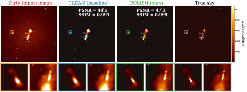
Figure 1: We propose a learning-based approach to recover a super-resolved astronomical image from a “dirty” input image captured by a radio interferometer. Our method, “POLISH” (green), outperforms the image-plane CLEAN algorithm (blue) on realistic simulations of radio images. Training data was significantly different from the radio sky image used in this example (training images were composed entirely of simple elliptical Gaussian shapes; see Section 4.1), but POLISH is still able to recover structured sources in the image. POLISH resolves finer spatial structures and achieves higher PSNR and SSIM than CLEAN. Data are normalized between 0 and 1 then raised to the power of 0.85 to better visualize faint structures. Each image is 0.26$\times$0.26 degrees.

High-resolution imaging of astronomical radio sources plays a critical role in studying our Universe. However, a fundamental challenge of high resolution imaging is that resolution is limited by aperture size (i.e., dish or mirror diameter), rendering single-dish telescopes insufficient in many cases. Alternatively, a radio interferometer is an array of antennas whose radio waves are coherently combined to obtain high resolution images (Ryle & Vonberg, 1946). Radio interferometry allows one to synthesize a much larger aperture, with the angular resolution now defined by the longest “baseline”, i.e. greatest separation, $D$, between antennas (Thompson et al., 1986; Burke & Graham-Smith, 1996). The diffraction limit of an interferometric array is given by $\theta\approx\lambda/D$, where $\lambda$ is observing wavelength. Probing scales below this limit is known as “super-resolution”. Interferometry has led to countless new discoveries where single-dish instruments were inadequate, including the first-ever direct image of a black hole (Event Horizon Telescope Collaboration, et al., 2019) and the precise localization of extragalactic transients (Hallinan et al., 2017; Ravi et al., 2019).

Recovering an image of the sky from an interferometer requires solving an ill-posed deconvolution problem. In particular, the placement of antennas in the interfometer defines a point spread function (PSF) that corrupts the true astronomical image. Preeminent observatories such as the Karl G. Jansky Very Large Array (VLA) and Atacama Large Millimeter/submillimeter Array (ALMA) have 27 and 66 radio antennas, respectively. In contrast, the upcoming Deep Synoptic Array in the Big Smoky Valley, Nevada, will contain and combine an unprecedented 2000 antennas . The DSA-2000’s impressive number of antennas corresponds to a PSF that can be more easily deconvolved, resulting in images with higher fidelity, higher dynamic range, and lower uncertainty. This “radio camera” will be the most powerful radio survey instrument to date and is expected to increase the known sample of astronomical radio sources by a factor of 1000.

The DSA-2000, which will yield unparalleled image quality, will also result in massive computational challenges: the telescope will need to churn through over 80 Tb/s of data. Unlike past radio interferometers that can save data to disk for later analysis, it will be impossible for the DSA-2000 to save raw data to disk. Specifically, the telescope will not preserve its visibility data. It is therefore essential that imaging on DSA-2000 be made fast, automated, and deterministic. Past methods for radio interferometric imaging are either too slow, require a human-in-the-loop, or result in sub-optimal image quality. Thus, it is critical that automated, feed-forward approaches be developed to transform quickly raw dirty images into high-fidelity reconstructions of the radio sky. We capitalize on recent advances in deep learning to develop an imaging pipeline for the DSA-2000 that can be used to deliver science-ready astronomical images in quasi-real time.

It is also essential that DSA-2000 be able to achieve super-resolution. With a PSF width of roughly 3 ”, many of the $\sim$ 10⁹ star forming radio galaxies (SFGs) detected by DSA-2000 will be unresolved in the dirty image. If these distant galaxies can be resolved with super-resolution, we will be able to carry out a powerful cosmological weak lensing survey on DSA-2000. By number of sources, such a survey is competitive with upcoming Stage IV optical weak-lensing experiments. Radio weak lensing is also highly complementary to upcoming optical surveys because the gravitational lensing signal is achromatic, whereas systematics will be different across wavelengths (Harrison et al., 2016; Camera et al., 2017). We therefore have a strong incentive to not only develop a robust feed-forward imaging framework, but one that provides super-resolution.

In this work, we demonstrate that recent advances in the classical problems of single-image super-resolution (SISR) and deconvolution through efficient neural network architectures make such imaging with the DSA-2000 possible. This manuscript is organized as follows. We first offer background on interferometric imaging, the DSA-2000, and the connection to SISR and deconvolution in Section 2. We then describe our deep learning based approach in Section 3, which we call POLISH (a demonstration is shown in Fig. 1). As we show, POLISH enables imaging at angular resolutions on the sky below the intrinsic resolution of the interferometric telescope array ($\approx$ 3 arcseconds for DSA-2000). Results based on simulated DSA-2000 data as well as on real astronomical data from the VLA are presented in Section 4. Where previous algorithms were made to deconvolve dirty images from sparse arrays, POLISH was designed to deconvolve images that are already relatively clean, hence its name. However, our demonstration on VLA data has shown that POLISH is a generic radio interferometric deconvolution procedure. In Section 5, we show how super-resolution on DSA-2000 will enable a powerful weak lensing survey. Finally, we discuss other scientific applications and show how feed-forward imaging could transform radio astronomy in coming years.

2 Background

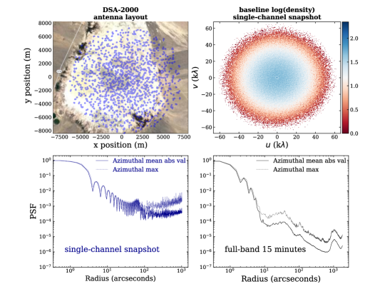
Figure 2: For our primary training set, we used the DSA-2000 layout shown here. The top left panel shows antenna position assumed for our simulation overlaid on Big Smoky Valley, Nevada. The top right panel shows the array’s UV coverage for a single frequency at a single time, represented as the logarithm of baseline density. The bottom two panels show an azimuthal average and maximum of the absolute value PSF for a single-channel snapshot (left) and the full band 15-minute integration (right). We expect the DSA-2000 layout to be further optimized for sidelobe suppression and azimuthal smoothness before it is built.

2.1 Interferometric imaging

In radio interferometry, each pair of antennas measures a Fourier coefficient of the underlying astronomical image, where the spatial frequency probed is related to the projected baseline between the antennas as well as the observing wavelength. Imaging then requires solving an inverse problem: recover the true sky image, $I_{\mathrm{sky}}$, using finite, and often sparse, spatial frequency measurements. Given enough antennas, one could densely sample the entire spatial frequency plane. In the absence of noise, these complex measurements, known as “visibilities” $V$, could then be used to recover an image through an inverse Fourier transform:

$$I_{\mathrm{sky}}=\mathcal{F}^{-1}\left(V\right).$$ (1)

Since we only have access to a finite number of spatial frequency Fourier coefficients in practice (i.e. a finite number of antennas pairs and finite range of radio frequencies), we do not have full access to $V$. We mathematically represent this by applying a sampling function, $S$, to the noisy measurements in the Fourier plane,

$$I_{\mathrm{d}}=\mathcal{F}^{-1}\left((V+n_{\rm vis})\,S\right),$$ (2)

where $n_{\rm vis}$ represents independent Gaussian noise at each spatial frequency and $I_{\mathrm{d}}$ is known as the “dirty image”. Invoking the convolution theorem, we can rewrite this equation as

$$I_{\mathrm{d}}=\mathcal{F}^{-1}\left(V\right)\otimes\,\mathcal{F}^{-1}\left(S\right)+n_{\rm sky},$$ (3)

where $\otimes$ denotes convolution and $n_{\rm sky}=\mathcal{F}^{-1}\left(n_{\rm vis}\right)\otimes\,\mathcal{F}^{-1}\left(S\right)$. The inverse Fourier transform of the sampled visibilities, $I_{\mathrm{d}}$, is degraded by the sampling function. By noting that the Fourier transform of our sampling function is just the instrument’s PSF, we can replace $\mathcal{F}^{-1}\left(S\right)$ with a convolution kernel $k$. This kernel depends not only on the telescope configuration but also the radio bandwidth, as can be seen in Figure 4. Finally, we are free to choose a pixelization scheme such that the resolution of the recovered image, $\hat{I}_{\mathrm{sky}}$, is $s$ times higher resolution than $I_{\mathrm{d}}$. By substituting Eq. 1, we obtain a mathematical description of the noisy and low-resolution image obtained by the interferometer, $I_{\mathrm{d}}$, as a function of our target, $I_{\mathrm{sky}}$:

$$I_{\mathrm{d}}=\left(I_{\mathrm{sky}}\otimes\,k\right)\downarrow_{s}+n_{\rm sky},$$ (4)

where $\downarrow_{s}$ is a downsampling operation. The inversion is challenging because for every $I_{d}$ there exist an infinite number of $I_{\mathrm{sky}}$ that would satisfy Eq. 4: i.e., interferometric deconvolution is an ill-posed inverse problem. It is also difficult for computational reasons, as the large spatial extent of the PSF, or kernel $k$, require large input and output images.

The goal of our work is to learn this mapping such that Eq. 4 can be inverted and an estimate for the true sky, $\hat{I}_{\mathrm{sky}}$, can be automatically recovered with a single pass through a neural network.

2.2 The Deep Synoptic Array (DSA-2000)

The Deep Synoptic Array, i.e., DSA-2000, is an ambitious new instrument expected to be complete by 2026 (Hallinan et al., 2019). It will survey the radio universe with unprecedented speed and depth, but this power comes at the expense of serious computational challenges. The DSA-2000 will consist of 2000$\times$5 m dual-polarization antennas observing the sky between 0.7 and 2.0 GHz. By the Nyquist–Shannon sampling theorem, the DSA-2000 must sample the electric field at more than 4 billion times per second, resulting in a raw data rate of over 10 TB/s. At the next stage in the pipeline, a single image of the sky produced using 15-minutes of visibility measurements requires $\approx$ 20 TB of data. This tremendous data rate prevents the use of imaging algorithms that store data and iteratively transform from visibilities in the Fourier plane to images in the sky plane. Instead, computational resources require that the DSA-2000 imaging pipeline rapidly recover an image of $I_{\mathrm{sky}}$ from $I_{\mathrm{d}}$ directly. In our proposed method, POLISH, we have developed a feed forward approach to invert a 2,000$\times$2,000 pixel image, $I_{\mathrm{d}}$, into a sky reconstruction, $\hat{I}_{\mathrm{sky}}$, in just a few seconds on a laptop.

2.3 Prior interferometric imaging techniques

Over the past half-century, considerable effort has been put into radio interferometric image reconstruction. While significant progress has been made, state-of-the-art algorithms do not satisfy the requirements for efficient super-resolution imaging on the DSA-2000. Imaging algorithms can be broadly categorized into two methodologies: CLEAN deconvolution and regularized maximum likelihood (RML) approaches.

CLEAN The de facto standard image reconstruction algorithm used in radio astronomy is known as CLEAN (Högbom, 1974; Clark, 1980). CLEAN attempts to iteratively deconvolve the PSF kernel $k$ from ${I}_{\mathrm{d}}$ to recover $I_{\mathrm{sky}}$, by assuming the sky is made up of a collection of point-sources. At each step, single pixels are added to a sky model at the locations of bright pixels in ${I}_{\mathrm{d}}$. The model pixels are scaled by the brightness of the corresponding pixels in ${I}_{\mathrm{d}}$. The sky model is then convolved with a Gaussian “restoring beam” to provide a smooth estimate of the recovered image. This final blurring step, necessitated by the point-source assumption in CLEAN, precludes CLEAN from recovering high spatial frequencies. This is because the restoring beam smooths data to the angular scale of the central component of the PSF. Besides not being able to deliver super-resolution, standard iterative algorithms like CLEAN introduce severe imaging artifacts near very bright or diffuse radio sources (see Fig. 8). There are variants on the standard Högbom CLEAN algorithm that allow for better reconstruction of diffuse or structured images, such as multi-scale CLEAN that are less sensitive to the point-source assumption (Wakker & Schwarz, 1988; Cornwell, 2008). In this paper we focus on standard image-plane CLEAN, as that is the likely alternative algorithm to POLISH that would be used on a radio camera such as DSA-2000.

Regularized Maximum Likelihood Regularized Maximum Likelihood (RML) methods are Bayesian inspired techniques that solve for an image by minimizing an objective function, which includes a term that penalizes poor data fit and an image regularization term (Wiaux et al., 2009; Bouman et al., 2016; Sun & Bouman, 2020). Some image regularization terms employed include maximum entropy (Cornwell & Evans, 1985; Narayan & Nityananda, 1986), total variation, and $\ell_{1}$ sparsity (Pratley et al., 2018). RML methods have had recent success in the radio interferometry community in their use for reconstructing the first image of a black hole, M87* (Event Horizon Telescope Collaboration, et al., 2019). Since RML methods do not rely on the CLEAN assumption that the sky is composed of point-sources, they can achieve super-resolution (Abdulaziz et al., 2019). However, they are very computationally expensive since they are iterative and model every measurement in the visibility domain. Though RML methods provide a more natural way of achieving super-resolution than CLEAN, these algorithms are not well suited for the DSA-2000 where fast, feed-forward image reconstruction is essential.

2.4 Deconvolution & single image super-resolution

Deconvolution is a classic inverse problem that aims to reconstruct a sharp image by removing an imaging system’s PSF from its measured blurry image (Riad, 1986; Starck et al., 2002). Traditional approaches to deconvolution include Weiner filtering and regularized inversion, however recently deep learning approaches have demonstrated impressive results on the task (Xu et al., 2014; Yan & Shao, 2016). Single image super-resolution (SISR) is an ill-posed inverse problem in which one attempts to obtain a high-resolution (HR) output from its corresponding low-resolution (LR) image (Glasner et al., 2009; Yang et al., 2014). Here too, deep learning based approaches to SISR have made significant progress, and efficient neural network architectures continue to be developed to learn the mapping between the high- and low-resolution images (Dong et al., 2015; Ledig et al., 2017; Yang et al., 2019). SISR shares conceptual similarities with deconvolution, since one can frame the SISR problem as removing the downsampling operation’s PSF from the image. However, unlike deconvolution, the mismatch in dimensions between the desired HR and input LR image causes the inverse problem to be ill-posed. The challenge of image reconstruction in radio interferometry can be formulated as a joint deconvolution and SISR inverse problem. In fact, replacing $I_{\mathrm{d}}/I_{\mathrm{sky}}$ with $I_{\mathrm{LR}}/I_{\mathrm{HR}}$ in Eq. 4 reproduces the generalized SISR image degradation equation used in (Yang et al., 2019).

There are nonetheless four critical differences between standard deconvolution-SSIR and astronomical imaging with radio interferometers. First, images of the radio sky require large dynamic ranges. In the annual New Trends in Image Restoration and Enhancement (NTIRE) data challenge for SISR, the image pairs were RGB 8-bit precision and roughly 2,000$\times$2,000 pixels. A typical 1 $\deg^{2}$ field on the sky measured with the DSA-2000 radio interferometer will have $\sim$ 20,000 unique sources with a range of brightness values approaching five orders of magnitude. Thus, we require at least 16-bit integers or preferably, 32-bit floats. Second, both the sky and instrument response are dependent on observing frequency. We therefore prefer multifrequency input data with an arbitrary number of channels, a generalization of the three color channels used for RGB images. Third, the PSF in radio astronomy can be highly spatially extended, unlike the simple Gaussian blurring kernel or bi-cubic downsampling typically assumed in many super-resolution applications. The PSF can also have significant radial and azimuthal structure (refer to Fig. 4). Fourth, while the response of our instrument is knowable in principle, calibration errors and other systematics lead to perturbations of the PSF. Therefore, our neural network must learn not just a single kernel, but a physically realistic distribution of PSFs (akin to partially blind deconvolution).

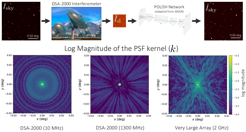
Figure 3: A schematic of the POLISH method of image reconstruction. The top row shows how the true sky is transformed by a radio interferometer and then recovered by our neural network. The bottom three figures show the PSF kernels used in this work: the DSA-2000 with just 10 MHz of its bandwidth used (left), and the full-band (1300 MHz) PSF of the DSA-2000 (middle), and an example VLA array configuration (right). Note that these kernels are plotted over the same extents as the observed sky images, highlighting that the kernels cause artifacts from bright sources that extend over the entire images.

3 Methods

The application of neural networks to super-resolution and deconvolution aims to learn the mapping between an input (convolved, lower-resolution) image and the true, higher-resolution image. This is done by training the neural network with a large number of image pairs ($I_{d}$/$I_{\mathrm{sky}}$ in our case) such that, when fed an input image the network can reproduce an accurate reconstruction of $I_{\mathrm{sky}}$. The training process penalizes any disagreement between the reconstructed image $\hat{I}_{\mathrm{sky}}$ and the true image, $I_{\mathrm{sky}}$, through its “loss function”. In effect, the neural network learns deconvolution. Radio interferometric imaging is therefore a natural application of the striking recent advances in learning-based deconvolution and super-resolution.

We modify the previously proposed Wide Activation for Efficient and Accurate Image Super-Resolution (WDSR) (Yu et al., 2018) architecture to allow for high-dynamic range and multifrequency input/output data, as well as to handle uncertainty in the PSF. This architecture is shown in Fig. 4. Our adaptation, POLISH, takes as input a dirty image, $I_{\mathrm{d}}$: a tensor with dimension ($n_{x}$, $n_{y}$, $n_{f}$) where $n_{x}$ and $n_{y}$ are spatial dimensions and $n_{f}$ is the number of frequency channels. POLISH outputs a super-resolved reconstruction of the sky, $\hat{I}_{\mathrm{sky}}$, whose shape is ($s\,n_{x}$, $s\,n_{y}$, $n_{f}$). Here, $s$ is the upsampling factor and takes values 2 or 3 in our work. The architecture depends on a residual network design with a single global skip connection and a residual block called “WDSR_b”. The final operation before the global skip connection and the primary path are summed is known as a pixel shuffle. These layers upsample the image by a factor of $s$, using a sub-pixel convolution with stride $1/s$ (Shi et al., 2016). To ensure high dynamic range deconvolution, POLISH now accepts as input 16-bit, or 32-bit data.

We train the POLISH network, $G_{\theta}$, on $N$ image pairs $\left(I_{\mathrm{d}}^{(n)},I_{\mathrm{sky}}^{(n)}\right)$, related through Eq. 4, to minimize an $\ell_{1}$ loss:

$$\hat{\theta}=\arg\min_{\theta}\sum_{n}\left|\left|I_{\mathrm{sky}}^{(n)}-G_{\theta}\left(I_{\mathrm{d}}^{(n)}\right)\right|\right|_{1}$$ (5)

The model is trained with roughly $10^{6}$ total epochs and a constantly decaying learning rate between $10^{-3}$ to $5\times 10^{-4}$. After each 1000 epochs of training, the model is tested on 10 images from the validation set, and a checkpoint is saved if its PSNR has improved. For results presented in this main paper, we use 800 image pairs for our training data and 100 pairs in our validation set. Each model takes roughly 20 GPU hours to train using an NVIDIA TITAN RTX GPU with 24 GB of memory. Before PSNR is calculated, or an $I_{\rm d}$ is fed to POLISH, data are normalized such that the image’s pixel values fall between 0 and 2${}^{n_{\rm bit}}$-1.

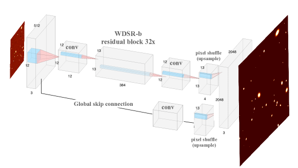
Figure 4: The neural network architecture that we have adapted for radio imaging, based on WDSR (Yu et al., 2018). A dirty image is fed to the network as an input and its output is a deconvolved reconstruction of the sky with $s$ times greater resolution in each direction. The network relies on residual blocks and a global skip connection. Batch normalization is removed.

3.1 Learning a PSF distribution

In radio interferometry an idealized PSF kernel is known a priori, as it is simply the inverse Fourier transform of the sampling function, $k_{\mathrm{ideal}}=\mathcal{F}^{-1}(S)$. However, in practice the instrumental response will cause the PSF to deviate from the ideal model due to, e.g., calibration errors. We therefore want the POLISH network to learn a distribution of PSFs, rather than a single PSF kernel. We build this into our training set by randomly perturbing the PSF in physically motivated ways when generating training image pairs. In particular, for each training pair the dirty image is created by applying a kernel that has been transformed in the following way,

$$k=\Lambda_{3}(\phi)\Lambda_{2}(\gamma)\Lambda_{1}(\alpha)\,k_{\mathrm{ideal}}.$$ (6)

These three transformations include a radial stretch, $\Lambda_{1}(\alpha):r\rightarrow\alpha\,r$ where the PSF shape is conserved but its size varies by tens of percent; this degradation is motivated by ionospheric effects that broaden the kernel but never shrinks it (i.e., $\alpha$ is drawn from (0,1])) (Intema et al., 2009). $\Lambda_{2}(\gamma)$ warps the PSF with random distortions (Smirnov, 2011), characterized by a parameter $\gamma$, as seen in Fig 7. Finally, an affine transformation $\Lambda_{3}(\phi)$ both contorts the PSF and a shifts it with a spatial translation, similar to what occurs when a telescope is mispointed.

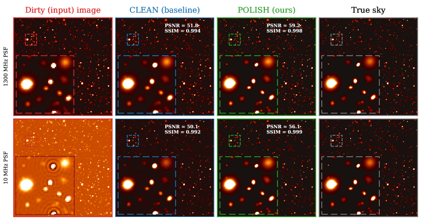
Figure 5: A simulated DSA-2000 interferometric observation of distant radio galaxies and the image reconstruction by image-plane CLEAN (middle left) and POLISH (middle right). The bottom row shows the sky convolved with DSA-2000’s PSF using less than 1$\%$ (single-channel snapshot); this case is critical for HI and OH science. The top row PSF uses the full-band with 15-minutes of integration and has a more complete sampling in the Fourier plane. In both cases POLISH outperforms the image-plane CLEAN baseline, especially for the 10 MHz PSF where substantial artifacts exist in the CLEAN reconstruction. The brightness of each image is independently scaled for visualization purposes.

3.2 Loss function and performance metric

We have tried training our model using $L^{1}$ and $L^{2}$ loss functions. Both are pixel-wise loss functions that measure the mean absolute error and mean squared error between input and output images, respectively. We find that the $L^{1}$ loss gives better results in terms of time for training to converge, in line with previous EDSR and WDSR networks (Lim et al., 2017; Yu et al., 2018). The final results presented here were trained using $L^{1}$ loss.

As a way of assessing the veracity of our reconstructed image and the performance of our neural network, we use two metrics. The first is peak signal-to-noise ratio ($PSNR$), which a standard statistic used in computer vision. PSNR is a pixel-by-pixel estimator of the ratio of maximum signal and corrupting image noise, expressed in decibels. It is given by,

$$PSNR=20\log{\left(\frac{MAX_{I}}{MSE}\right)},$$ (7)

where $MAX_{I}$ is the maximum possible pixel value in an image, and $MSE$ is the mean squared error across all pixels. For an 8-bit RGB image, $MAX_{I}$ is 255. In general, it is $2^{N_{\rm b}}-1$ where $N_{\rm b}$ is the number of bits per sample. The $MSE$ is calculated as the average square difference between the true image and the super-resolved image ($I_{\rm SR}$), given by,

$$MSE=\frac{1}{N_{l}\,N_{m}}\sum_{l}\sum_{m}\left(I_{\rm sky}(l,m)-I_{\rm SR}(l,m)\right)^{2}.$$ (8)

$PSNR$ depends on pixel-wise error, making it sensitive to translations of the image, or “astrometric error” in our case. Since we are concerned here with small distortions to galaxy shapes, we also employ a more perception-based metric known as the structural similarity index measure ($SSIM$) (Wang et al., 2004). $SSIM$ compares various windows within an image to asses the statistics of those regions, rather than directly computing absolute differences in pixels. For two boxes $x$ and $y$ with dimensions $N\times N$,

$$SSIM(x,y)=\frac{(2\mu_{x}\mu_{y}+c_{1})(2\sigma_{xy}+c_{2})}{(\mu_{x}^{2}+\mu_{y}^{2}+c_{1})(\sigma_{x}^{2}+\sigma_{y}^{2}+c_{2})}$$ (9)

Here $\mu$ is the mean of that box, $\sigma^{2}$ is variance, $\sigma_{xy}$ is covariance, and $c_{1}$ and $c_{2}$ are two variables to stabilize the division with weak denominator. We use both $SSIM$ and $PSNR$ to test the performance of POLISH.

4 Experimental setup & results

The performance of POLISH is assessed on both realistic simulations mimicking data from the DSA-2000, as well as real experimental data from the VLA at 2–4 GHz. We compare the POLISH reconstruction with image-plane CLEAN and the true image (in the case of simulated sky data), using both PSNR and SSIM to quantify reconstruction quality. These are summarized in Table 1.

4.1 Synthetic training data

We model the radio sky and measurement noise to simulate a physically realistic training set. This is done by first simulating a $\sim$2,000$\times$2,000 pixel image of the true sky, $I_{\mathrm{sky}}$ with a field of view of $\sim$0.3$\times$0.3 deg. DSA-2000 will primarily detect radio galaxies with a detection rate corresponding to an average of 13,000 galaxies per square degree above a signal-to-noise (SNR) of 6 (Hallinan et al., 2019). We populate each realization of $I_{\mathrm{sky}}$ with $N$ sources, where $N$ is randomly drawn from a Poisson distribution whose mean is 13,000 times the sky coverage in degrees. The galaxies are 2D Gaussian ellipsoids with random orientation angles on the sky. The statistics of their brightness, ellipticity, and angular size are chosen to match the empirically measured distributions for radio galaxies (Tunbridge et al., 2016). The galaxy peak flux values range from a few to several thousand $\mu$Jy/pixel. Finally, we model the spectral index of each source with a Gaussian distribution centered on -0.55 and with standard deviation 0.25, based on the observed spectra of SFGs near the DSA-2000 band, 0.7–2 GHz (Tisanić et al., 2019).

A dirty image, $I_{\mathrm{d}}$, corresponding to each true sky image is obtained through the process mathematically described in Eq. 4. The PSF kernel used to degrade $I_{\mathrm{sky}}$ is obtained by sampling from Eq. 6. The unperturbed PSF is computed for each telescope configuration using the packages casa (McMullin et al., 2007) and wsclean (Offringa et al., 2014). Before applying the PSF kernel to obtain $I_{\mathrm{d}}$, zero-mean i.i.d. Gaussian noise with a standard deviation $\sigma_{\mathrm{sky}}$ is applied to mimic $n_{\mathrm{sky}}$. The convolved image is then downsampled by a factor $s$. The parameters $\sigma_{\mathrm{sky}}=0.5$ $\mu$Jy/pixel and $s=3$ are used to simulate DSA-2000 dirty images, while values of $\sigma_{\mathrm{sky}}=3$ $\mu$Jy/pixel and $s=2$ are used for generating VLA training data used in Section 4.2.3.

Results presented in the main paper consist of 16-bit single-channel input data, where a multifrequency dependence has been included in the PSF kernel but not $I_{\mathrm{sky}}$. On DSA-2000, we use two PSFs: one that uses the full radio bandwidth (1300 MHz) with 15 minutes of earth-rotation synthesis and one that uses just  $\sim$ 1$\%$ of the observing bandwidth (a narrow 10 MHz range of wavelengths) for a single snapshot, shown in Fig. 3. If the PSF is generated across multiple frequencies, it is effectively averaged over the band to produce a single channel.

4.2 Results

Figure 1 visually compares the performance of POLISH against the baseline CLEAN algorithm on synthetic DSA-2000 observations, using an SKA Data Challenge image as $I_{\rm sky}$ (Bonaldi et al., 2021). The input dirty image, corresponding to a 1300 MHz bandwidth PSF, is shown on the left. Although POLISH was only trained on images with Gaussian sources, it is able to recover more complex underlying sharp structure. As demonstrated by the increase in PSNR and SSIM, POLISH recovers a substantially improved image compared to both the measured dirty image and the CLEAN reconstruction, at nearly 3 dB higher than the latter. Image-plane CLEAN produces more speckle and sidelobe artifacts than POLISH, leading to false-positive detections of radio galaxies in our simulation. For example, Source-Extractor tends to find approximately one false-positive galaxy per twenty simulated galaxies in the CLEAN reconstruction, whereas the POLISH neural network “hallucinates” just one source per fifty true galaxies.

Figure 5 shows a visual example of POLISH results on DSA-2000 synthetic data, comparing results on data generated with a 10 MHz and 1300 MHz bandwidth PSF. In order to best see the improvement, each panel shows a zoom-in on a 0.06 $\deg\times$0.06 $\deg$ region of the full simulated sky, where dozens of radio galaxies with different sizes, shapes, and orientations can be seen. In the 10 MHz bandwidth PSF, less than $1\%$ of the available radio wavelengths are used to construct the PSF; reconstructing an image with only a small portion of the full PSF bandwidth is important for HI and OH studies on DSA-2000. This region of the sky has two particularly bright “galaxies”, which makes the PSF visible in the 10 MHz bandwidth dirty image.

Bandwidth (MHz)	$PSNR$ (POLISH)	$PSNR$ (CLEAN)	$SSIM$ POLISH	$SSIM$ CLEAN
1300	55.9$\pm 4.7$	50.0$\pm 6.0$	0.998$\pm$0.0016	0.989$\pm$0.007
10	55.1$\pm 3.8$	47.4$\pm 3.6$	0.988$\pm$0.0016	0.976$\pm$0.009

Table 1: Results from image reconstruction comparison between CLEAN and POLISH for the full-band case (1300 MHz) and the single-channel scenario (10 MHz). POLISH achieves a higher Peak Signal-to-Noise Ratio (PSNR) and structural similarity index measure (SSIM) than CLEAN, indicating better pixel-wise and perceptual fidelity, respectively.

In both cases POLISH substantially outperforms the CLEAN baseline. POLISH achieves a mean PSNR$=$55.9$\pm 4.7$ and SSIM$=$0.998$\pm$0.0016 for our radio galaxy simulation with the 1300 MHz PSF on 50 validation images, compared with PSNR$=$50.0$\pm 6.0$ and SSIM$=$0.989$\pm$0.007 on CLEAN. The 10 MHz PSF results in PSNR$=$55.1$\pm 3.8$ and SSIM$=$0.988$\pm$0.0016 using POLISH. For CLEAN this was PSNR$=$47.4$\pm 3.6$ and SSIM$=$0.976$\pm$0.009. These results are presented in Table 1.

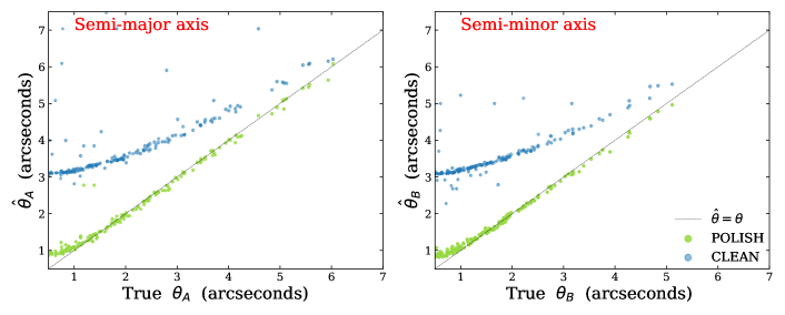
Figure 6: A comparison of the resolving power of POLISH (green dots) with that of traditional CLEAN algorithm (blue dots) on simulated DSA-2000 data with a 1300 MHz PSF kernel. The vertical axes are the fitted semi-major (left) and semi-minor (right) axes, $\hat{\theta}$, of hundreds of “galaxies” in the reconstructed images. They are plotted against the true galaxy sizes in arcseconds. CLEAN’s resolving power asymptotes to the PSF angular scale preventing it from achieving super-resolution, while POLISH achieves accurate super-resolution well below the intrinsic resolution of the interferometer ($\approx 3$ arcseconds). Note that we have not pushed the limits of POLISH’s super-resolution because in this simulation the smallest galaxies approach the pixel scale in size.

4.2.1 Super-resolution

Super-resolution is critical for many scientific goals of the DSA-2000. We therefore investigate if spatial scales below the width of the PSF’s central lobe ($\approx 3$ arcseconds) can be reliably accessed with POLISH. We quantify the super-resolution capability of POLISH using the galaxy simulations described in Section 4.1. First, the size of each “galaxy” is extracted using the astronomical fitting software Source-Extractor (Bertin & Arnouts, 1996). This is done on the true image, CLEAN image, and the POLISH image. The fitted galaxy sizes are then compared on a source-by-source basis; for each galaxy, we contrast the input (true sky) and output (POLISH and CLEAN reconstructions) semi-major ($\theta_{A}$) and semi-minor axes ($\theta_{B}$). If the reconstructed value, $\hat{\theta}$, is below the PSF angular scale of $\approx 3$ arcseconds, then super-resolution has been achieved. As can be seen in Fig. 6, galaxies in the POLISH image are consistently the same size as galaxies in the true image, even at sub-arcsecond scales well below the DSA-2000’s PSF size. In contrast, the traditional CLEAN algorithm cannot achieve super-resolution and instead asymptotes to the PSF central component’s angular size.

4.2.2 Model mismatch

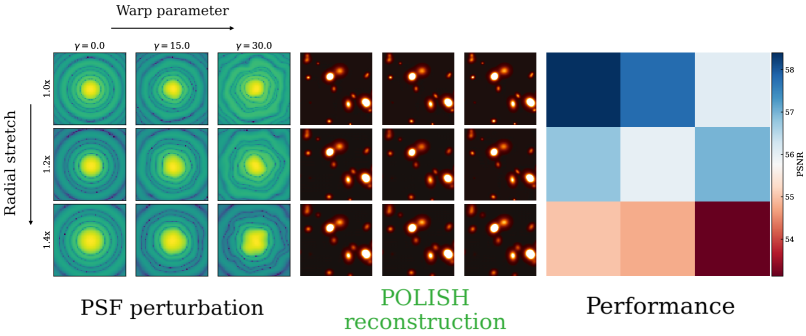
Figure 7: The impact of model mismatch on reconstruction performance. POLISH has been trained using a distribution of PSF kernels with warps in the range of $\gamma$=0 to 20. We then validate on dirty images that have been corrupted by a PSF kernel that has been radially stretched (increasing downwards) and warped (increasing to the right), the logarithm of which is shown on the left (zoomed in on the PSF’s inner 28$\times$28 arcseconds). The corresponding POLISH images and PSNRs are shown in the middle and right, respectively.

When a distribution of PSFs are used during training, POLISH can more robustly reconstruct the sky in the presence of instrumental calibration errors. We have performed an ablation study showing how performance decreases when training data is restricted to images corrupted with the ideal PSF kernel $k_{\mathrm{ideal}}$.

In Fig. 7 we demonstrate POLISH image reconstruction on test data whose PSF has been perturbed outside of the range of training data pertubations. In particular, POLISH has been trained with PSF kernels transformed by the warp function $\Lambda_{2}(\gamma)$ described in Section 3.1, with $\gamma$ drawn from a uniform distribution between 0 and 20. The training data PSFs were not radially stretched for this figure, allowing us to test POLISH’s performance under model mismatch. As can be seen in the PSNR performance plot, the quality of the recovered test images degrades as the PSF perturbations get larger than the training set distortions. However, even in the relatively extreme distortions (bottom right element of each 3$\times$3 grid) PSNR remains above 50 (and comparable to or better than the typical CLEAN-based PSNRs above). Such distortions and uncertainty in the DSA-2000 PSF are greater than what we expect for actual experimental data; it is unlikely that the true PSF will be $40\%$ larger than the modelled PSF, and distortions as severe as the $\gamma=30$ “warp” would require drastic mis-calibration.

4.2.3 Deconvolving real astronomical data

In practise, POLISH will be trained offline on simulated data and then applied to real data in quasi-real time. We show that POLISH can reliably deconvolve real observations, having only been trained on simulations. To demonstrate this, real astronomical observations (Hallinan et al., 2017) were obtained from the VLA, a Y-shaped, 27-telescope interferometer in New Mexico, including a modelled PSF for that observation’s configuration. We then trained POLISH on our radio galaxy simulation described in Sect. 4.1, but with $I_{d}$/$I_{sky}$ image pairs created with the VLA PSF.

Reconstructing the sky from VLA data is a more challenging problem than what we will be faced with at DSA-2000, as it has far fewer antennas and therefore a much more degraded PSF (Fig. 4). Evidenced by the strong artifacts in the dirty image of Fig. 8, the VLA’s PSF is much less suppressed off-axis than that of DSA-2000. The PSF is also highly azimuthally asymmetric due to the Y-shape of the array, leading to six radial “struts” expanding outwards from each source in the dirty image.

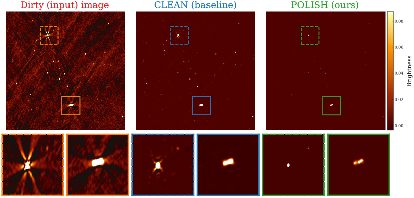
Figure 8: An example of POLISH being applied to real astronomical data from the Very Large Array (VLA), having been trained only on simulated data. The left panel shows the “dirty image” as measured by the VLA, and the right two panels show the traditional CLEAN algorithm’s (middle) and our proposed approach POLISH (right). Specifically, these are the image reconstructions obtained by the two distinct deconvolution algorithms.

In Fig. 8 we demonstrate that POLISH can deconvolve the real VLA dirty image, leaving behind fewer imaging artifacts than the traditional image-plane CLEAN algorithm. Fig. 8 shows a comparison of the dirty (input) image, CLEAN reconstruction, and POLISH reconstruction (left to right) for a 0.1$\times$0.1 $\deg$ region of the 0.4$\times$0.4 $\deg$ full image, including a further zoom in on particularly bright radio galaxies (bottom row). The difference between CLEAN and POLISH for the bright galaxies is striking. CLEAN leaves behind residual structures from the PSF, whereas POLISH produces shapes like those expected for distant radio galaxies. These residual structures include speckles that are likely not real radio point sources, as they lie in a line on the struts of the PSF response from bright galaxies; this is consistent with our the increased false-positive rate of CLEAN vs. POLISH in our simulated sky reconstruction.

We have chosen not to compare POLISH with RML methods for the following reasons. There exists a wide spectrum of RML algorithms and a true comparison would require comparing POLISH against a large set of reconstructions, each with its own finely tuned set of regularization parameters; some would perform poorly, some may do well, depending on our choice of parameters. We therefore cannot construct an apples-to-apples comparison that would meaningfully contrast an efficient, feed-forward algorithm such as POLISH with RML methods.

This result is very promising for two reasons. First, we have shown that a relatively simple simulated data set can train a neural network that will deconvolve real radio inteferometric data. Second, the VLA’s sampling of the Fourier plane is much less complete than that of DSA-2000. The fact that POLISH can still perform under these circumstances shows that deep learning based techniques are not only a promising solution for the DSA-2000, but also for other current and future radio interferometers (Jonas & MeerKAT Team, 2016; Hotan et al., 2021; Dewdney et al., 2009).

5 Radio weak lensing & DSA-2000

Weak gravitational lensing is a powerful probe of the Universe’s composition and expansion history, and is an essential tool for constraining the physical nature of dark energy (Kaiser, 1998; Hoekstra & Jain, 2008; Mandelbaum, 2018). Weak lensing imparts a distortion on distant galaxy shapes known as “shear”, causing a separation-dependent correlation between galaxy shapes that is determined by the Universe’s large scale structure and its evolution with time. Measuring the power spectrum of this cosmic shear allows us to constrain the cosmological parameters. To date, weak lensing research has been significantly more advanced at optical wavelengths. However, the achromaticity of gravitational lensing means the large scale structure will imprint itself the same way across the electromagnetic spectrum, while the systematics across wavelengths will vary. Observations in different bands are therefore highly complementary. For a detailed treatment of radio weak lensing in the context of the Square Kilometer Array (SKA) see (Brown et al., 2015; Harrison et al., 2016; Bonaldi et al., 2016; Camera et al., 2017).

In the radio, few surveys thus far have had sufficient angular resolution, sensitivity, and sky coverage to detect the large numbers of SFGs required to do weak lensing cosmology. Using $\sim$ 9$\times 10^{5}$ sources in the FIRST survey at 1.4 GHz, Chang et al. (2004) fit galaxies in UV space to make the first-ever radio detection of weak lensing. Demetroullas & Brown (2016) cross-correlated an optical shear map containing $\sim$ 9 million galaxies in the Sloan Digital Sky Survey (SDSS) with a radio shear map from FIRST, resulting in a 2.7 $\sigma$ detection of weak lensing. More recently, the SuperCLASS survey used 0.26 deg² of radio data from eMERLIN and the VLA, as well as 1.53 deg² of optical data from the Subaru telescope, but had too few sources to make a detection (Harrison et al., 2020). Despite the required catch-up at long wavelengths, there are benefits to doing weak lensing in the radio. For example, the PSF of a radio interferometer can be known a priori through forward modelling, which is not true for optical telescopes. Furthermore, as both optical and radio lensing experiments will likely be systematics limited, cross-correlation provides a robust and unbiased estimator of the shear powerspectrum (Camera et al., 2017; Harrison et al., 2020). And finally, sensitive radio telescopes such as DSA-2000 and the SKA are expected to probe higher redshifts than comparable optical surveys, with a fatter tail at high $z$.

The DSA-2000 will survey the whole sky north of declination $-30^{\circ}$ between 0.7 and 2.0 GHz down to a root-mean square (RMS) noise of just 0.5 $\mu$Jy. The survey will contain approximately $10^{9}$ sources, primarily star forming radio galaxies. This is over one thousand times more galaxies than the FIRST sample where a radio weak lensing signal was first detected (Chang et al., 2004), and with a much cleaner PSF than the VLA (see Fig. 4). However, with a point spread function (PSF) whose full-width at half maximum (FWHM) is roughly 3”, many radio galaxies will be unresolved for the DSA-2000 in the dirty image. Using POLISH to achieve super-resolution, DSA-2000 could be competitive and complementary with Stage IV weak lensing experiments such as Euclid and the Vera C. Rubin Observatory. Shear maps from DSA-2000 will therefore enable a symbioses between wavelengths, where cross-correlating radio/optical shear maps allow for tight constraints on both dark energy and modified gravity (Harrison et al., 2016).

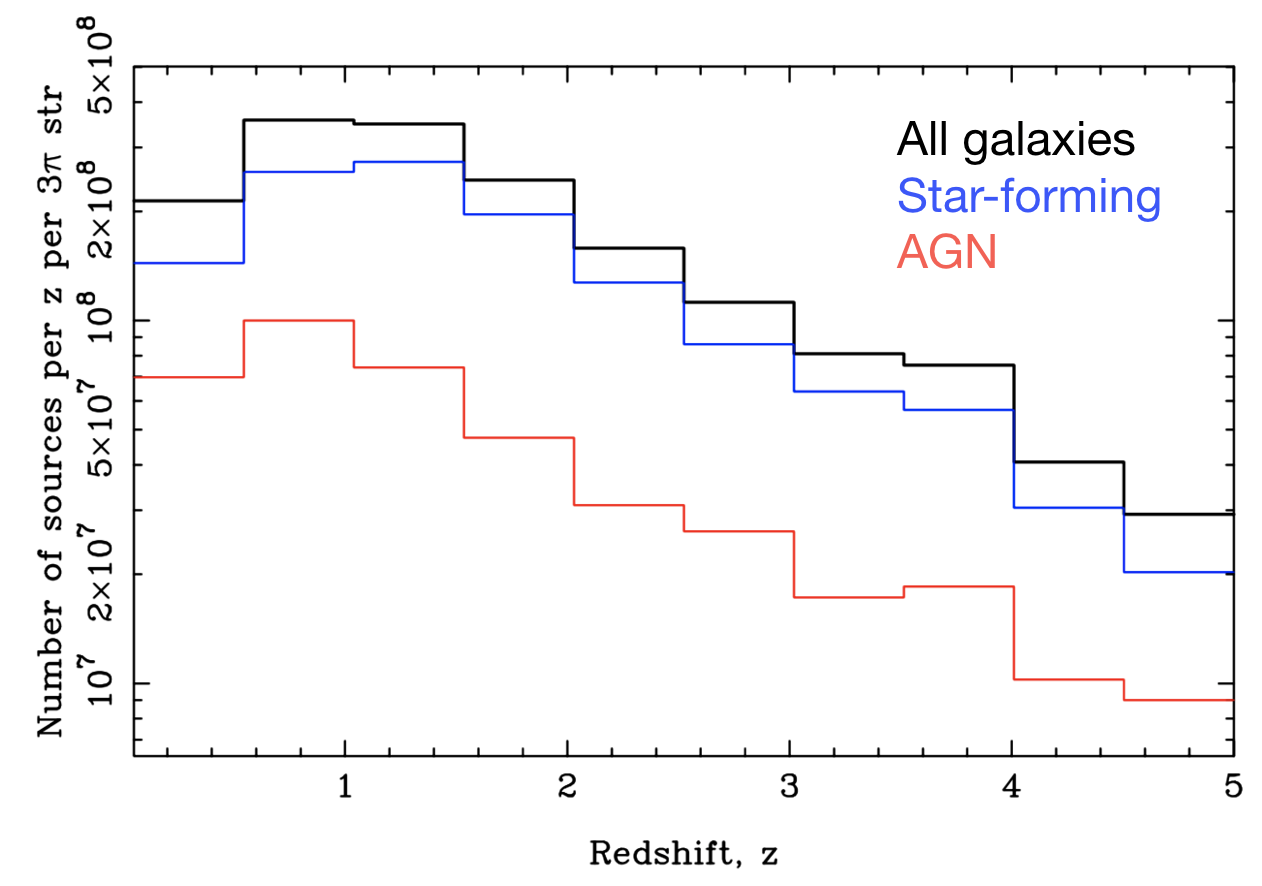
Figure 9: DSA-2000 will detect an enormous number of star forming galaxies. These can be used for weak lensing cosmology if resolution below the telescope’s PSF width can be achieved.

5.1 Radio weak lensing systematics

Shape noise on the shear powerspectrum falls in proportion to the number of galaxies in the survey. But systematic uncertainties will play a large role in upcoming weak lensing surveys, whether in the radio or optical. For example, the intrinsic alignment of galaxies can break the assumption that galaxy position angles and shapes are inherently uncorrelated. Biases in the measurement of shear must be accounted for and carefully calibrated out, as well as uncertainty in redshift estimation (Mandelbaum, 2018). Finally, the PSF must be deconvolved out of the image, and residual PSF errors will lead to galaxy shape distortions. In the case of ground-based optical telescopes, time-variable seeing and related systematics make PSF modelling a central effort in weak lensing analysis (Gatti et al., 2021; Jarvis et al., 2021).

In the radio, weak lensing experiments suffer from overlapping but distinct systematics. Intrinsic alignment bias will affect galaxies in any weak lensing survey, but can potentially be calibrated out in the radio using the polarized emission of star forming galaxies, which is unaltered by lensing (Brown & Battye, 2011; Harrison et al., 2016). The PSF of a radio interferometer can be modelled deterministically (see Section 2.1), in contrast to an optical telescope. But PSF modelling is still a source of significant uncertainty because the PSF of an interferometer is typically poorly behaved, with significant sidelobes and azimuthal structure thanks to sparse sampling of the aperture. This makes image reconstruction, and therefore shear measurement, more sensitive to errors in the PSF model even if the response can be forward modelled.

The DSA-2000 will skirt some of these issues by densely sampling the UV plane and by optimizing antenna configuration to produce an azimuthally smooth PSF and highly attenuated sidelobes. While its suppressed sidelobes and smoothness will reduce errors introduced by PSF modelling and deconvolution, the nominal beam size of 3” means that many SFGs will have angular size below our diffraction limit, hence our requirement of super-resolution. The DSA-2000 will therefore have fewer image reconstruction relics that bias galaxy shape measurement, but will be limited by resolution. For reference, the Dark Energy Survey has a median seeing of roughly 1” and has produced strong cosmological constraints from its weak lensing experiment (Gatti et al., 2021), which sets an achievable baseline for POLISH.

5.2 Forecasting

We would like to estimate how well a weak-lensing survey on DSA-2000 will be able to constrain the cosmological parameters, both in the case where super-resolution of a factor of a few is achieved (POLISH SR in Table 2) and when spatial resolution is limited by the synthesised beam size of 3” (No SR in Table 2). We compare simulations for DSA-2000 with simulations of SKA1 and the Euclid. Euclid is a visible to near-infrared space telescope expected to launch in mid- to late-2022 and is considered a Stage IV experiment. For these forecasts we use the same parameters assumed by Harrison et al. (2016). SKA1 will be a mixed array of 133 15 m SKA dishes and 64 13.5 m dishes from the MeerKAT telescope and a nominal PSF of 0.5”. Its weak lensing survey will be on Band 2 at 0.95–1.76 GHz (Harrison et al., 2016). As an empirical benchmark, we take the recently-published Dark Energy Survey (DES) Year 3 Results (DES Collaboration et al., 2021). DES is a Stage III experiment that is already producing cosmological strong constraints from its optical weak lensing survey. We show these survey parameters in Table 2.

Survey	$N_{gal}$	Sky coverage (deg2)	$n_{gal}$ (sq arcmin-1)	$f_{z}$	$\sigma_{pz}$
DSA-2000: POLISH SR	109	32,000	6/3†	0.3	0.05
DSA-2000: No SR	109	32,000	6/0.5†	0.3	0.05
SKA1	5$\times 10^{7}$	5,000	2.7	0.15	0.05
Euclid	1.6$\times 10^{9}$	15,000	30	0.33	0.04
DES Y3	$10^{8}$	4,143	6.7/5.6†	0.0	0.05

Table 2: Parameters used for forecasting the constraining power of a weak lensing experiment on different surveys, including DSA-2000 with and without POLISH’s super-resolution. $N_{gal}$ is the total number of detections, $n_{gal}$ is the on-sky density, $f_{z}$ is the fraction of galaxies with spectroscopic redshift, and $\sigma_{pz}$ is the uncertainty on photometric redshifts. The DES Y3 row corresponds to the real values obtained from the year 3 galaxy shape catalog (Gatti et al., 2021); the other rows are estimates of survey parameters.
$\dagger$ Effective aerial number density of galaxies. On DSA-2000 we assume that only half of galaxies will be sufficiently super-resolved to produce a shape measurement.

We base our estimate of the effective number of usable galaxies on both the estimated PSF sizes and the observed distribution of galaxy sizes. Owen & Morrison (2008) find that half of SFGs above 15 $\mu$Jy have major-axes greater than 1”. However, recent work has argued that $\mu$Jy radio sources may be more compact than previously believed, with a median FWHM of 0.3” (Cotton et al., 2018; Jiménez-Andrade et al., 2021). For this reason, we assume that only one half of sources will be resolved with POLISH, assuming an effective resolution of 3”/SNR. For the case where super-resolution is not achieved we assume under 10$\%$ of sources will be resolved. For this reason we take the effective areal density for DSA-2000 with POLISH to be 3 galaxies per square arcminute, while only 0.5 galaxies per square arcminute will be useable without super-resolution. We assume that SKA1 will be able to resolve $\mathcal{O}(1)$ of detected galaxies, so we do not adjust its $n_{gal}$. The same is true for Euclid, which is space-based and therefore diffraction limited at its nominal resolution of 0.2”.

Forecasting weak lensing constraints requires each survey’s expected redshift distribution, areal density of galaxies, $n_{gal}$, total sky coverage, and information about the error in lensed galaxy redshifts. Obtaining redshifts of the lensed galaxies is an important component of weak lensing, as the cross-correlation angular powerspectra between different redshift bins offers information on the evolution of structure over cosmic time (Bonnett et al., 2016). For this analysis, we follow Harrison et al. (2016) in using the MCMC parameter estimation code CosmoSIS (Zuntz et al., 2015). Specifically, we use code they have developed for forecasting the SKA’s radio weak lensing survey, but with the putative DSA-2000 parameters (Hallinan et al., 2019). On DSA-2000, we assume 15$\%$ of source will have spectroscopic redshifts (i.e. zero redshift uncertainty). The error on photometric redshifts will be approximately 0.05. DSA-2000 will obtain galaxy redshifts using several different methods. Approximately 30 million galaxies at $z<1$ will have spectroscopic redshifts from the DSA’s HI survey. The SPHEREx near-infrared all-sky survey (Doré et al., 2014) will determine the redshifts of over one billion galaxies with $\sigma_{z}/(1+z)\leq 10\%$ and a subset of several hundred million galaxies with $\sigma_{z}/(1+z)\leq 1\%$ (see here for current forecasts). Of these, three quarters can be cross-matched with the DSA-2000 catalog.

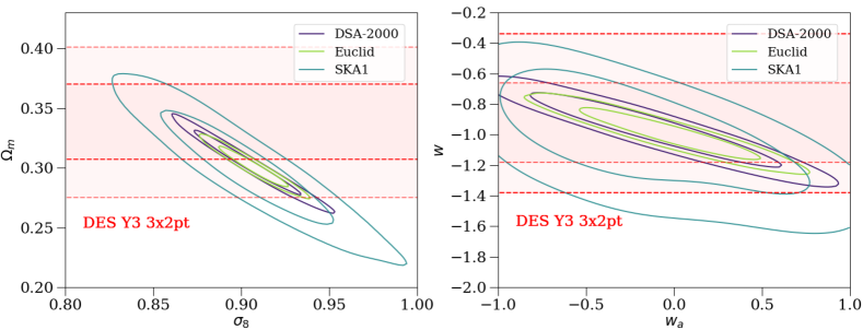
Figure 10: Marginalized constraints on dark energy equation of state parameters, $w$ and $w_{a}$ (left), and matter powerspectrum parameters, $\Omega_{m}$ and $\sigma_{8}$ (right) for weak lensing surveys on DSA-2000 (with super-resolution), Euclid, and SKA1. The red shaded regions are the 1- and 2-$\sigma$ constraints from the Dark Energy Survey Year 3 (DES Y3 3x2pt) data after combining three two-point correlation functions (cosmic shear, galaxy clustering, and shear with lens galaxy positions) (DES Collaboration et al., 2021). Note that the forecasts for DSA-2000, Euclid, and SKA1 are cosmic shear only, but do not include lensing systematics.

We focus here on DSA-2000’s ability to constrain the matter density and matter power spectrum normalization, $\Omega_{m}$ and $\sigma_{8}$ respectively, as well as the dark energy equation of state parameters $w$ and $w_{a}$. In Fig. 10 we show the cosmological parameter posteriors produced by CosmoSIS for DSA-2000, Euclid, and SKA1. The red regions show the 1- and 2-$\sigma$ constraints from DES Y3 results. We use their three two-point (3x2pt) correlation functions in cosmic shear, galaxy clustering, and shear with lens galaxy positions (DES Collaboration et al., 2021). We find that SKA1’s weak lensing survey will be comparable to the DES 3x2pt constraints in constraining both the matter powerspectrum and dark energy. DSA-2000 produces constraints that are nearly as tight as Euclid. All four surveys provide an excellent opportunity for cross-correlation and cross-validation, particularly between the different wavelengths (Harrison et al., 2016; Camera et al., 2017).

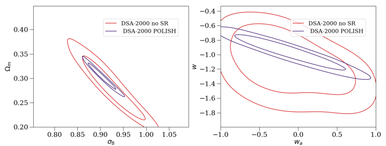
Figure 11: Comparing the ability of weak lensing survey on DSA-2000 to constrain the cosmological parameters with (purple) and without (red) POLISH’s super-resolution.

6 Discussion & conclusion

We have developed and demonstrated POLISH: a high dynamic range residual neural network for fast, accurate and super-resolved astronomical imaging with radio interferometers. Feed forward approaches like POLISH will be essential in analyzing data from upcoming instruments with enormous data rates where stream processing is critical, such as the upcoming DSA-2000 (Hallinan et al., 2019). We have shown that POLISH is highly effective at deconvolving the PSF in both simulated and real astronomical data. It also achieves super-resolution and outperforms the interferometric deconvolution algorithm of the last five decades, image-plane CLEAN, in both reconstruction accuracy (PSNR and SSIM) and resolution. We have shown how method forward-modelling approaches such as RML are not a viable option for surveys such as DSA-2000, where data rates preclude the preservation of visibilities. In its current form, POLISH (like CLEAN) does not provide uncertainty in image reconstruction. Looking forward, we plan to estimate uncertainty in the reconstructed image within the POLISH framework using Baysian deep learning to produce a posterior for $\hat{I}_{\rm sky}$.

Besides addressing the deconvolution problem in radio-interferometric images, POLISH makes possible new, currently inaccessible science by achieving super-resolution. When applied to data from the DSA-2000, POLISH will allow shape measurements of nearly $\sim$ 10⁹ galaxies, enabling a weak lensing survey. We have forecasted the DSA-2000’s ability to constrain cosmological parameters and compared it with both upcoming and current weak lensing experiments. We have also shown the significant improvement in constraints when achieving super-resolution with POLISH vs. when resolution is set by the diffraction limit.

For the specific application of weak lensing with POLISH, future work will benefit from a more detailed, forward modelled simulation of shear estimation systematics and PSF errors. Beyond the fraction of SFGs that can be resolved, it is important to know how different image reconstruction algorithms affect galaxy shapes as a function of S/N, galaxy size, redshift, and proximity to bright sources. This exercise would result in a mock galaxy shape catalog using one or more imaging techniques, including for other radio weak lensing experiments. For example, the SKA will be less constrained by resolution than DSA-2000, but may benefit from the learning-based, accurate reconstructions provided by POLISH. The MeerKAT International GHz Tiered Extragalactic Exploration (MIGHTEE) survey will achieve $\mu$Jy sensitivity over 20 deg² with a well-behaved PSF (Jarvis et al., 2016). Though its nominal 6” resolution is larger than most SFGs, MIGHTEE would provide an interesting application of POLISH to radio weak lensing. More generally, we anticipate that feed-forward techniques such as POLISH that deliver robust deconvolution and super-resolution will be valuable for upcoming high-volume radio surveys.

7 Data availability

The code for POLISH can be found at https://github.com/liamconnor/polish-pub/. This includes tools for simulating the microJansky radio sky as well as code to train and use the POLISH neural network.

References

- Abdulaziz et al. (2019) Abdulaziz, A., Dabbech, A., & Wiaux, Y. 2019, MNRAS, 489, 1230, doi: 10.1093/mnras/stz2117
- Bertin & Arnouts (1996) Bertin, E., & Arnouts, S. 1996, A&AS, 117, 393, doi: 10.1051/aas:1996164
- Bonaldi et al. (2016) Bonaldi, A., Harrison, I., Camera, S., & Brown, M. L. 2016, MNRAS, 463, 3686, doi: 10.1093/mnras/stw2104
- Bonaldi et al. (2021) Bonaldi, A., An, T., Brüggen, M., et al. 2021, MNRAS, 500, 3821, doi: 10.1093/mnras/staa3023
- Bonnett et al. (2016) Bonnett, C., Troxel, M. A., Hartley, W., et al. 2016, Phys. Rev. D, 94, 042005, doi: 10.1103/PhysRevD.94.042005
- Bouman et al. (2016) Bouman, K. L., Johnson, M. D., Zoran, D., et al. 2016, in The IEEE Conference on Computer Vision and Pattern Recognition (CVPR, 913. https://arxiv.org/abs/1512.01413
- Brown et al. (2015) Brown, M., Bacon, D., Camera, S., et al. 2015, in Advancing Astrophysics with the Square Kilometre Array (AASKA14), 23. https://arxiv.org/abs/1501.03828
- Brown & Battye (2011) Brown, M. L., & Battye, R. A. 2011, MNRAS, 410, 2057, doi: 10.1111/j.1365-2966.2010.17583.x
- Burke & Graham-Smith (1996) Burke, B. F., & Graham-Smith, F. 1996, An Introduction to Radio Astronomy
- Camera et al. (2017) Camera, S., Harrison, I., Bonaldi, A., & Brown, M. L. 2017, MNRAS, 464, 4747, doi: 10.1093/mnras/stw2688
- Chang et al. (2004) Chang, T.-C., Refregier, A., & Helfand, D. J. 2004, ApJ, 617, 794, doi: 10.1086/425491
- Clark (1980) Clark, B. G. 1980, A&A, 89, 377
- Cornwell (2008) Cornwell, T. J. 2008, IEEE Journal of Selected Topics in Signal Processing, 2, 793, doi: 10.1109/JSTSP.2008.2006388
- Cornwell & Evans (1985) Cornwell, T. J., & Evans, K. F. 1985, A&A, 143, 77
- Cotton et al. (2018) Cotton, W. D., Condon, J. J., Kellermann, K. I., et al. 2018, ApJ, 856, 67, doi: 10.3847/1538-4357/aaaec4
- Demetroullas & Brown (2016) Demetroullas, C., & Brown, M. L. 2016, MNRAS, 456, 3100, doi: 10.1093/mnras/stv2876
- DES Collaboration et al. (2021) DES Collaboration, Abbott, T. M. C., Aguena, M., et al. 2021, arXiv e-prints, arXiv:2105.13549. https://arxiv.org/abs/2105.13549
- Dewdney et al. (2009) Dewdney, P. E., Hall, P. J., Schilizzi, R. T., & Lazio, T. J. L. W. 2009, IEEE Proceedings, 97, 1482, doi: 10.1109/JPROC.2009.2021005
- Dong et al. (2015) Dong, C., Loy, C. C., He, K., & Tang, X. 2015, IEEE transactions on pattern analysis and machine intelligence, 38, 295
- Doré et al. (2014) Doré, O., Bock, J., Ashby, M., et al. 2014, arXiv e-prints, arXiv:1412.4872. https://arxiv.org/abs/1412.4872
- Event Horizon Telescope Collaboration, et al. (2019) Event Horizon Telescope Collaboration,, Akiyama, K., Alberdi, A., et al. 2019, ApJ, 875, L1, doi: 10.3847/2041-8213/ab0ec7
- Gatti et al. (2021) Gatti, M., Sheldon, E., Amon, A., et al. 2021, MNRAS, 504, 4312, doi: 10.1093/mnras/stab918
- Gatti et al. (2021) Gatti, M., Sheldon, E., Amon, A., et al. 2021, Monthly Notices of the Royal Astronomical Society, 504, 4312, doi: 10.1093/mnras/stab918
- Glasner et al. (2009) Glasner, D., Bagon, S., & Irani, M. 2009, in 2009 IEEE 12th international conference on computer vision, IEEE, 349–356
- Hallinan et al. (2017) Hallinan, G., Corsi, A., Mooley, K. P., et al. 2017, Science, 358, 1579, doi: 10.1126/science.aap9855
- Hallinan et al. (2019) Hallinan, G., Ravi, V., Weinreb, S., et al. 2019, in Bulletin of the American Astronomical Society, Vol. 51, 255. https://arxiv.org/abs/1907.07648
- Harrison et al. (2016) Harrison, I., Camera, S., Zuntz, J., & Brown, M. L. 2016, MNRAS, 463, 3674, doi: 10.1093/mnras/stw2082
- Harrison et al. (2020) Harrison, I., Brown, M. L., Tunbridge, B., et al. 2020, MNRAS, 495, 1737, doi: 10.1093/mnras/staa696
- Hoekstra & Jain (2008) Hoekstra, H., & Jain, B. 2008, Annual Review of Nuclear and Particle Science, 58, 99, doi: 10.1146/annurev.nucl.58.110707.171151
- Högbom (1974) Högbom, J. A. 1974, A&AS, 15, 417
- Hotan et al. (2021) Hotan, A. W., Bunton, J. D., Chippendale, A. P., et al. 2021, PASA, 38, e009, doi: 10.1017/pasa.2021.1
- Intema et al. (2009) Intema, H. T., van der Tol, S., Cotton, W. D., et al. 2009, A&A, 501, 1185, doi: 10.1051/0004-6361/200811094
- Jarvis et al. (2016) Jarvis, M., Taylor, R., Agudo, I., et al. 2016, in MeerKAT Science: On the Pathway to the SKA, 6. https://arxiv.org/abs/1709.01901
- Jarvis et al. (2021) Jarvis, M., Bernstein, G. M., Amon, A., et al. 2021, MNRAS, 501, 1282, doi: 10.1093/mnras/staa3679
- Jiménez-Andrade et al. (2021) Jiménez-Andrade, E. F., Murphy, E. J., Heywood, I., et al. 2021, ApJ, 910, 106, doi: 10.3847/1538-4357/abe876
- Jonas & MeerKAT Team (2016) Jonas, J., & MeerKAT Team. 2016, in MeerKAT Science: On the Pathway to the SKA, 1
- Kaiser (1998) Kaiser, N. 1998, The Astrophysical Journal, 498, 26
- Ledig et al. (2017) Ledig, C., Theis, L., Huszár, F., et al. 2017, in Proceedings of the IEEE conference on computer vision and pattern recognition, 4681–4690
- Lim et al. (2017) Lim, B., Son, S., Kim, H., Nah, S., & Mu Lee, K. 2017, in Proceedings of the IEEE Conference on Computer Vision and Pattern Recognition (CVPR) Workshops
- Mandelbaum (2018) Mandelbaum, R. 2018, Annual Review of Astronomy and Astrophysics, 56, 393
- McMullin et al. (2007) McMullin, J. P., Waters, B., Schiebel, D., Young, W., & Golap, K. 2007, in Astronomical Society of the Pacific Conference Series, Vol. 376, Astronomical Data Analysis Software and Systems XVI, ed. R. A. Shaw, F. Hill, & D. J. Bell, 127
- Narayan & Nityananda (1986) Narayan, R., & Nityananda, R. 1986, ARA&A, 24, 127, doi: 10.1146/annurev.aa.24.090186.001015
- Offringa et al. (2014) Offringa, A. R., McKinley, B., Hurley-Walker, N., et al. 2014, MNRAS, 444, 606, doi: 10.1093/mnras/stu1368
- Owen & Morrison (2008) Owen, F. N., & Morrison, G. E. 2008, AJ, 136, 1889, doi: 10.1088/0004-6256/136/5/1889
- Pratley et al. (2018) Pratley, L., McEwen, J. D., d’Avezac, M., et al. 2018, MNRAS, 473, 1038, doi: 10.1093/mnras/stx2237
- Ravi et al. (2019) Ravi, V., Catha, M., D’Addario, L., et al. 2019, Nature, 572, 352, doi: 10.1038/s41586-019-1389-7
- Riad (1986) Riad, S. 1986, Proceedings of the IEEE, 74, 82, doi: 10.1109/PROC.1986.13407
- Ryle & Vonberg (1946) Ryle, M., & Vonberg, D. D. 1946, Nature, 158, 339, doi: 10.1038/158339b0
- Shi et al. (2016) Shi, W., Caballero, J., Huszar, F., et al. 2016, in Proceedings of the IEEE Conference on Computer Vision and Pattern Recognition (CVPR)
- Smirnov (2011) Smirnov, O. M. 2011, A&A, 527, A107, doi: 10.1051/0004-6361/201116434
- Starck et al. (2002) Starck, J. L., Pantin, E., & Murtagh, F. 2002, Publications of the Astronomical Society of the Pacific, 114, 1051, doi: 10.1086/342606
- Sun & Bouman (2020) Sun, H., & Bouman, K. L. 2020, arXiv e-prints, arXiv:2010.14462. https://arxiv.org/abs/2010.14462
- Thompson et al. (1986) Thompson, A. R., Moran, J. M., & Swenson, G. W. 1986, Interferometry and synthesis in radio astronomy
- Tisanić et al. (2019) Tisanić, K., Smolčić, V., Delhaize, J., et al. 2019, A&A, 621, A139, doi: 10.1051/0004-6361/201834002
- Tunbridge et al. (2016) Tunbridge, B., Harrison, I., & Brown, M. L. 2016, MNRAS, 463, 3339, doi: 10.1093/mnras/stw2224
- Wakker & Schwarz (1988) Wakker, B. P., & Schwarz, U. J. 1988, A&A, 200, 312
- Wang et al. (2004) Wang, Z., Bovik, A. C., Sheikh, H. R., & Simoncelli, E. P. 2004, IEEE Transactions on Image Processing, 13, 600, doi: 10.1109/TIP.2003.819861
- Wiaux et al. (2009) Wiaux, Y., Jacques, L., Puy, G., Scaife, A. M. M., & Vandergheynst, P. 2009, MNRAS, 395, 1733, doi: 10.1111/j.1365-2966.2009.14665.x
- Xu et al. (2014) Xu, L., Ren, J. S., Liu, C., & Jia, J. 2014, Advances in neural information processing systems, 27, 1790
- Yan & Shao (2016) Yan, R., & Shao, L. 2016, IEEE Transactions on Image Processing, 25, 1910, doi: 10.1109/TIP.2016.2535273
- Yang et al. (2014) Yang, C.-Y., Ma, C., & Yang, M.-H. 2014, in European conference on computer vision, Springer, 372–386
- Yang et al. (2019) Yang, W., Zhang, X., Tian, Y., et al. 2019, IEEE Transactions on Multimedia, 21, 3106, doi: 10.1109/TMM.2019.2919431
- Yu et al. (2018) Yu, J., Fan, Y., Yang, J., et al. 2018, arXiv preprint arXiv:1808.08718
- Zuntz et al. (2015) Zuntz, J., Paterno, M., Jennings, E., et al. 2015, Astronomy and Computing, 12, 45, doi: 10.1016/j.ascom.2015.05.005