Coupled Cluster Downfolding Theory: towards efficient many-body algorithms for dimensionality reduction of composite quantum systems

Abstract

The recently introduced coupled cluster (CC) downfolding techniques for reducing the dimensionality of quantum many-body problems recast the CC formalism in the form of the renormalization procedure allowing, for the construction of effective (or downfolded) Hamiltonians in small-dimensionality sub-space, usually identified with the so-called active space, of the entire Hilbert space. The resulting downfolded Hamiltonians integrate out the external (out-of-active-space) Fermionic degrees of freedom from the internal (in-the-active-space) parameters of the wave function, which can be determined as components of the eigenvectors of the downfolded Hamiltonians in the active space. This paper will discuss the extension of non-Hermitian (associated with standard CC formulations) and Hermitian (associated with the unitary CC approaches) downfolding formulations to composite quantum systems. The non-Hermitian formulation can provide a platform for developing local CC approaches, while the Hermitian one can serve as an ideal foundation for developing various quantum computing applications based on the limited quantum resources. We also discuss the algorithm for extracting the semi-analytical form of the inter-electron interactions in the active spaces.

I Introduction

The coupled cluster (CC) methodology Coester (1958); Coester and Kummel (1960); Čížek (1966); Paldus, Čížek, and Shavitt (1972); Purvis and Bartlett (1982); Koch and Jørgensen (1990); Paldus and Li (1999); Crawford and Schaefer (2000); Bartlett and Musiał (2007) is a driving engine of high-precision simulations in physics, chemistry, and material sciences. Several properties of CC made it especially efficient in capturing correlation effects in many-body quantum systems ranging from quantum field theory, Funke, Kaulfuss, and Kümmel (1987); Kümmel (2001); Hasberg and Kümmel (1986); Bishop, Ligterink, and Walet (2006); Ligterink, Walet, and Bishop (1998) quantum hydrodynamics, Arponen et al. (1988); Bishop et al. (1989) and nuclear structure theory Dean and Hjorth-Jensen (2004); Kowalski et al. (2004); Hagen et al. (2008) to quantum chemistry Scheiner et al. (1987); Sinnokrot, Valeev, and Sherrill (2002); Slipchenko and Krylov (2002); Tajti et al. (2004); Crawford (2006); Parkhill, Lawler, and Head-Gordon (2009); Riplinger and Neese (2013); Yuwono, Magoulas, and Piecuch (2020) and material sciences. Stoll (1992); Hirata et al. (2004a); Katagiri (2005); Booth et al. (2013); Degroote et al. (2016); McClain et al. (2017); Wang and Berkelbach (2020); Haugland et al. (2020a) In this article, we will mainly focus our attention on the application to quantum chemistry. Many appealing features of the single-reference (SR) CC formalism (which will be the main focus of the present discussion) in applications to chemical systems originate in the exponential parametrization of the ground-state wave function and closely related linked cluster theorem.Brandow (1967); Lindgren and Morrison (2012); Shavitt and Bartlett (2009) The last feature assures the so-called additive separability of the calculated energies in the non-interacting sub-system limit, which plays a critical role in the proper description of various chemical transformations such as chemical reactions that include bond breaking and bond-forming processes. The linked cluster theorem also plays a crucial role in designing formalisms that can provide the chemical accuracy needed for predicting spectroscopic data, reaction rates, and thermochemistry data. The best-known example of such class of methods is the CCSD(T) formalism,Raghavachari et al. (1989) which combines the iterative character of the CCSD formalism Purvis and Bartlett (1982) (CC with single and double excitations) with perturbative techniques for determining CC energy corrections due to connected triple excitations. Over the last few decades, the CCSD(T)-type formulations have been refined to provide accurate description of bond-breaking processes. Among several formulations that made it possible were the method of moments of coupled cluster equations and renormalized approaches,Piecuch and Kowalski (2011); Kowalski and Piecuch (2000a, b); Piecuch and Włoch (2005); Cramer et al. (2006); Włoch, Gour, and Piecuch (2007); Piecuch, Gour, and Włoch (2009); Deustua, Shen, and Piecuch (2017); Deustua et al. (2018); Bauman, Shen, and Piecuch (2017) perturbative formulations based on the $\Lambda$-operator (defining the left eigenvectors of the similarity transformed Hamiltonians) Stanton (1997); Stanton and Gauss (1995); Crawford and Stanton (1998); Kucharski and Bartlett (1998a, b); Gwaltney and Head-Gordon (2000, 2001); Hirata et al. (2001); Bomble et al. (2005) and other techniques.Kucharski and Bartlett (1998c); Meissner and Bartlett (2001); Robinson and Knowles (2013); Bozkaya and Schaefer III (2012) One should also mention the tremendous effort in formulating reduced-scaling or local formulations of the CC methods to extend the applicability of the CC formalism across spatial scales.Hampel and Werner (1996); Schütz (2000); Schütz and Werner (2000, 2001); Li, Ma, and Jiang (2002); Li et al. (2006, 2009); Li and Piecuch (2010); Neese, Wennmohs, and Hansen (2009); Neese et al. (2009); Riplinger et al. (2016, 2013); Pavosevic et al. (2016) In several cases, the extension of local formulations was possible for linear response CC theory D’Cunha and Crawford (2020) and excited state CC formulations based on the equation-of-motion formalism. Dutta, Neese, and Izsák (2016); Peng, Clement, and Valeev (2018)

Recently, interesting aspects of SR-CC were discussed using the sub-system embedding sub-algebras (SES) approach,Kowalski (2018, 2021) where we demonstrated that the CC energy can be calculated in an alternative way to the standard CC energy formula. Instead of using standard energy expression, one can obtain the same energy by diagonalizing the downfolded/effective Hamiltonian in method-specific active space(s) generated by appropriate sub-system embedding sub-algebras. The SR-CC theory provides a rigorous algorithm for how to construct these Hamiltonians using the external, with respect to the active space, class of cluster amplitudes.Kowalski (2018) Shortly after this discovery, these results for static SR-CC formulations were extended to the time domain.Kowalski and Bauman (2020) Following similar concepts as in the static case and assuming that the external time-dependent cluster amplitudes are known or can be effectively approximated, it was shown that the quantum evolution of the entire system can be generated in the active space by time-dependent downfolded Hamiltonian. Another interesting aspect of CC SES downfolding is the possibility of integrating several SES CC eigenvalue problems corresponding to various active spaces into a computational flow or quantum flow as discussed in Ref.Kowalski (2021), where we demonstrated that the flow equations are fully equivalent to the standard approximations given by cluster operators defined by unique internal excitations involved in the active-space problems defining the flow. This feature provides a natural language for expressing the sparsity of the system. In contrast to other local CC approaches, the CC quantum flow equations can effectively embrace the concept of localized orbital pairs at the level of effective Hamiltonian acting in the appropriate active space.

The SES CC downfolded Hamiltonians are non-Hermitian operators, which limits their utilization in quantum computing. Instead, using double unitary CC (DUCC) Ansatz,Bauman et al. (2019); Bauman, Low, and Kowalski (2019); Kowalski and Bauman (2020); Kowalski (2021) one can derive the active-space many-body form of Hermitian downfolded Hamiltonians. In contrast to the SR-CC, the DUCC-based effective Hamiltonians are expressed in terms of non-terminating expansions involving anti-Hermitian cluster operators defined by external type excitations/de-excitations. Several approximate forms of DUCC Hamiltonians have been tested in the context of quantum simulations, showing the potential of DUCC downfolding in reproducing exact ground-state energy in small active spaces.Bauman et al. (2019, 2020) In particular, the downfolded Hamiltonians have been integrated with various quantum solvers, including Variational Quantum Eigensolvers (VQE) Peruzzo et al. (2014); McClean et al. (2016); Romero et al. (2018); Shen et al. (2017); Kandala et al. (2017, 2019); Colless et al. (2018); Huggins et al. (2020); Cao et al. (2019) and Quantum Phase Estimation (QPE),Kitaev (1997); Nielsen and Chuang (2011); Luis and Peřina (1996); Cleve et al. (1998); Berry et al. (2007); Childs (2010); Seeley, Richard, and Love (2012); Wecker, Hastings, and Troyer (2015); Häner et al. (2016); Poulin et al. (2017) to calculate ground-state potential energy surfaces corresponding to breaking a single chemical bond.

In this paper, we will briefly review the current status of the downfolding methods and provide further extension of the CC downfolding methods to multi-component systems. As a specific example, we choose a composite system defined by Fermions of type A and Fermions of type B. This is a typical situation encountered for certain classes of non-Born-Oppenheimer dynamics and nuclear structure theory. The discussed formalism can be easily extended to other types of systems composed of Fermions and Bosons as encountered in the descriptions of polaritonic systems. We believe that these formulations will pave the way for more realistic quantum simulations of multi-component systems.

II CC theory

The SR-CC theory utilizes the exponential representation of the ground-state wave function $|\Psi\rangle$,

$$|\Psi\rangle=e^{T}|\Phi\rangle\;,$$ (1)

where $T$ and $|\Phi\rangle$ represent the so-called cluster operator and single-determinantal reference function. The cluster operator can be represented through its many-body components $T_{k}$

$$T=\sum_{i=1}^{M}T_{k}\;,$$ (2)

where individual component $T_{k}$ takes the form

$$T_{k}=\frac{1}{(k!)^{2}}\sum_{i_{1},\ldots,i_{k};a_{1},\ldots,a_{k}}t^{i_{1}\ldots i_{k}}_{a_{1}\ldots a_{k}}E^{a_{1}\ldots a_{k}}_{i_{1}\ldots i_{k}}\;,$$ (3)

where indices $i_{1},i_{2},\ldots$ ($a_{1},a_{2},\ldots$) refer to occupied (unoccupied) spin orbitals in the reference function $|\Phi\rangle$. The excitation operators $E^{a_{1}\ldots a_{k}}_{i_{1}\ldots i_{k}}$ are defined through strings of standard creation ($a_{p}^{\dagger}$) and annihilation ($a_{p}$) operators

$$E^{a_{1}\ldots a_{k}}_{i_{1}\ldots i_{k}}=a_{a_{1}}^{\dagger}\ldots a_{a_{k}}^{\dagger}a_{i_{k}}\ldots a_{i_{1}}\;,$$ (4)

where creation and annihilation operators satisfy the following anti-commutation rules:

$$[a_{p},a_{q}]_{+}=[a_{p}^{\dagger},a_{q}^{\dagger}]_{+}=0\;,$$ (5)

$$[a_{p},a_{q}^{\dagger}]_{+}=\delta_{pq}\;.$$ (6)

When $M$ in the summation in Eq. (2) is equal to the number of correlated electron ($N_{e}$) then the corresponding CC formalism is equivalent to the FCI method, otherwise for $M<N_{e}$ one deals with the standard approximation schemes. Typical CC formulations such as CCSD, CCSDT, and CCSDTQ correspond to $M=2$, $M=3$, and $M=4$ cases, respectively.

The equations for cluster amplitudes $t^{i_{1}\ldots i_{k}}_{a_{1}\ldots a_{k}}$ and ground-state energy $E$ can be obtained by introducing Ansatz (1) into the Schrödinger equation and projecting onto $P+Q$ space, where $P$ and $Q$ are the projection operator onto the reference function and the space of excited Slater determinants obtained by acting with the cluster operator onto the reference function $|\Phi\rangle$, i.e.,

$$(P+Q)He^{T}|\Phi\rangle=E(P+Q)e^{T}|\Phi\rangle\;,$$ (7)

where $H$ represents the electronic Hamiltonian. The above equation is the so-called energy-dependent form of the CC equations, which corresponds to the eigenvalue problem only in the exact wave function limit when $T$ contains all possible excitations. Approximate CC formulations do not represent the eigenvalue problem. At the solution, the energy-dependent CC equations are equivalent to the energy-independent or connected form of the CC equations:

$$Qe^{-T}He^{T}|\Phi\rangle = 0\;,$$ (8)

$$\langle\Phi|e^{-T}He^{T}|\Phi\rangle = E\;.$$ (9)

Using Baker-Campbell-Hausdorff (BCH) formula and Wick’s theorem one can show that only connected diagrams contribute to Eqs.(8) and (9). For notational convenience, one often uses the similarity transformed Hamiltonian $\bar{H}$, defined as

$$\bar{H}=e^{-T}He^{T}\;.$$ (10)

III Non-Hermitian CC downfolding

The main idea of SR-CC non-Hermitian downfolding hinges upon the characterization of sub-systems of a quantum system of interest in terms of active spaces or commutative sub-algebras of excitations that define corresponding active space. This is achieved by introducing sub-algebras of algebra $\mathfrak{g}^{(N)}$ generated by $E^{a_{l}}_{i_{l}}=a_{a_{l}}^{\dagger}a_{i_{l}}$ operators in the particle-hole representation defined with respect to the reference $|\Phi\rangle$. As a consequence of using the particle-hole formalism, all generators commute, i.e., $[E^{a_{l}}_{i_{l}},E^{a_{k}}_{i_{k}}]=0$, and algebra $\mathfrak{g}^{(N)}$ (along with all sub-algebras considered here) is commutative. The CC SES approach utilizes class of sub-algebras of commutative $\mathfrak{g}^{(N)}$ algebra, which contain all possible excitations $E^{a_{1}\ldots a_{m}}_{i_{1}\ldots i_{m}}$ needed to generate all possible excitations from a subset of active occupied orbitals (denoted as $R$, $\{R_{i},\;i=1,\ldots,x_{R}\}$) to a subset of active virtual orbitals (denoted as $S$, $\{S_{i},\;i=1,\ldots,y_{s}\}$) defining active space. These sub-algebras will be designated as $\mathfrak{g}^{(N)}(R,S)$. Sometimes it is convenient to use alternative notation $\mathfrak{g}^{(N)}(x_{R},y_{S})$ where numbers of active orbitals in $R$ and $S$ orbital sets, $x_{R}$ and $y_{S}$, respectively, are explicitly called out. As discussed in Ref.Kowalski, 2018, configurations generated by elements of $\mathfrak{g}^{(N)}(x_{R},y_{S})$, along with the reference function, span the complete active space (CAS) referenced to as the CAS($R,S$) (or equivalently CAS($\mathfrak{g}^{(N)}(x_{R},y_{S})$)).

In Refs. Kowalski, 2018; Kowalski and Bauman, 2020; Kowalski, 2021, we explored the effect of partitioning of the cluster operator induced by general sub-algebra $\mathfrak{h}=\mathfrak{g}^{(N)}(x_{R},y_{S})$, where the cluster operator $T$, given by Eq. (2), is represented as

$$T=T_{\rm int}(\mathfrak{h})+T_{\rm ext}(\mathfrak{h})\;,$$ (11)

where $T_{\rm int}(\mathfrak{h})$ belongs to $\mathfrak{h}$ while $T_{\rm ext}(\mathfrak{h})$ does no belong to $\mathfrak{h}$. If the expansion $T_{\rm int}|\Phi\rangle$ produces all Slater determinants (of the same symmetry as the $|\Phi\rangle$ state) in the active space, we call $\mathfrak{h}$ the sub-system embedding sub-algebra for the CC formulation defined by the $T$ operator. In Ref. Kowalski, 2018, we showed that each CC approximation has its own class of SESs.

A direct consequence of existence of the SESs for standard CC approximations is the fact that the corresponding energy can be calculated, in an alternative way to Eq. (9), as an eigenvalue of the active-space non-Hermitian eigenproblem

$$H^{\rm eff}(\mathfrak{h})e^{T_{\rm int}(\mathfrak{h})}|\Phi\rangle=Ee^{T_{\rm int}(\mathfrak{h})}|\Phi\rangle\;.$$ (12)

where

$$H^{\rm eff}(\mathfrak{h})=(P+Q_{\rm int}(\mathfrak{h}))\bar{H}_{\rm ext}(\mathfrak{h})(P+Q_{\rm int}(\mathfrak{h}))\;$$ (13)

and

$$\bar{H}_{\rm ext}(\mathfrak{h})=e^{-T_{\rm ext}(\mathfrak{h})}He^{T_{\rm ext}(\mathfrak{h})}\;.$$ (14)

In Eq.(13) the projection operator $Q_{\rm int}(\mathfrak{h})$ is a projection operator on a sub-space spanned by all Slater determinants generated by $T_{\rm int}(\mathfrak{h})$ acting onto $|\Phi\rangle$.

Since in the definition of the effective Hamiltonian, Eqs. (13) and (14), only $T_{\rm ext}(\mathfrak{h})$ is involved, one can view the SES CC formalism with the resulting active-space eigenvalue problem, Eq. (12), as a specific form of renormalization procedure where external parameters defining the corresponding wave function are integrated out. One should also mention that calculating the CC energy as an eigenvalue problems, as described by Eq. (12), is valid for any SES for a given CC approximation given by cluster operator $T$. According to this general result, the standard CC energy expression, shown by Eq. (9), can be reproduced when one uses trivial sub-algebra, which contains no excitations (i.e., active space contains $|\Phi\rangle$ only).

The existence of alternative ways of calculating CC energy opens alternative ways of constructing new classes of approximations. For example, if one integrates several eigenvalues problems corresponding to SESs $\mathfrak{h}_{i},\;(i=1,\ldots,M)$ into a quantum flow equations (QFE) discussed in Ref. Kowalski, 2021, i.e.,

$$H^{\rm eff}(\mathfrak{h}_{i})e^{T_{\rm int}(\mathfrak{h}_{i})}|\Phi\rangle=Ee^{T_{\rm int}(\mathfrak{h}_{i})}|\Phi\rangle\;(i=1,\ldots,M)\;.$$ (15)

In Ref. Kowalski, 2018 we demonstrated that at the solution, the solution of the QFE is equivalent to the solution of standard CC equations in the form of Eqs. (8) and (9) defined by cluster operator $T$ which is a combination of all unique excitations included in $T_{\rm int}(\mathfrak{h}_{i})$ $(i=1,\ldots,M)$ operators. This is can be symbolically expressed as

$$T=\bigcup_{i=1}^{M}T_{\rm int}(\mathfrak{h}_{i})\;.$$ (16)

These two equivalent representations allows one also to form the following important corollary:
Corollary (or the equivalence theorm) For certain forms of cluster operator $T$, the standard connected form of the CC equations given by Eqs. (8) and (9) can be replaced by quantum flow equations composed of non-Hermitian eigenvalue problems, Eq. (15).
The above corollary plays an important role in defining reduced-scaling formulations. This is a consequence of the fact that each sub-problem corresponding to sub-algebra $\mathfrak{h}_{i}$ has the associated form of the effective Hamiltonian $H^{\rm eff}(\mathfrak{h}_{i})$, which allows to define one body-density matrix for the sub-system and select the sub-set of the most important cluster amplitudes in the $T_{\rm int}(\mathfrak{h}_{i})$ operator. For example, when a localized orbital basis set is used, this procedure can be used to define the so-called orbital pairs at the level of the effective Hamiltonian, which is a significant advantage compared to the existing local CC approaches. This procedure can also be extended to other systems driven by different types of interactions such as in nuclear structure theory or quantum lattice models, where the extension of the standard local CC formulations as used in quantum chemistry is not obvious.

IV Hermitian CC Downfolding

In order to employ downfolding methods in quantum simulations, one has to find a way to construct Hermitian effective Hamiltonians. This goal can be achieved by employing the double unitary coupled Ansatz (DUCC),Kowalski and Bauman (2020) where the ground-state wave function is represented as

$$|\Psi\rangle=e^{\sigma_{\rm ext}(\mathfrak{h})}e^{\sigma_{\rm int}(\mathfrak{h})}|\Phi\rangle\;,$$ (17)

where $\sigma_{\rm ext}(\mathfrak{h})$ and $\sigma_{\rm int}(\mathfrak{h})$ are general-type anti-Hermitian operators

$$\sigma_{\rm int}^{\dagger}(\mathfrak{h}) = -\sigma_{\rm int}(\mathfrak{h})\;,$$ (18)

$$\sigma_{\rm ext}^{\dagger}(\mathfrak{h}) = -\sigma_{\rm ext}(\mathfrak{h})\;.$$ (19)

In analogy to the SR-CC case, all cluster amplitudes defining $\sigma_{\rm int}$ cluster operator carry active indices only (or indices of active orbitals defining given $\mathfrak{h}$). The external part $\sigma_{\rm ext}(\mathfrak{h})$ is defined by amplitudes carrying at least one inactive orbital index. However, in contrast to the SR-CC approach, internal/external parts of anti-Hermitian cluster operators are not defined in terms of excitations belonging explicitly to a given sub-algebra, but rather by indices defining active/inactive orbitals specific to a given $\mathfrak{h}$. Therefore $\mathfrak{h}$ will be used here in the context of CAS’s generator. Another difference with the SR-CC downfolding lies in the fact that while for the SR-CC cases components of cluster operators $T_{\rm int}(\mathfrak{h})$ and $T_{\rm ext}(\mathfrak{h})$ were commuting as a consequence of particle-hole formalism employed, in the unitary case, the operators forming $\sigma_{\rm int}(\mathfrak{h})$ and $\sigma_{\rm ext}(\mathfrak{h})$ are non-commuting.

Employing DUCC Ansatz, Eq. (17), one can show that in analogy to the SR-CC case, the energy of the entire system (once the exact form of $\sigma_{\rm ext}(\mathfrak{h})$ operator is known) can be calculated through the diagonalization of the effective/downfolded Hamiltonian in SES-generated active space, i.e.,

$$H^{\rm eff}(\mathfrak{h})e^{\sigma_{\rm int}(\mathfrak{h})}|\Phi\rangle=Ee^{\sigma_{\rm int}(\mathfrak{h})}|\Phi\rangle,$$ (20)

where

$$H^{\rm eff}(\mathfrak{h})=(P+Q_{\rm int}(\mathfrak{h}))\bar{H}_{\rm ext}(\mathfrak{h})(P+Q_{\rm int}(\mathfrak{h}))$$ (21)

and

$$\bar{H}_{\rm ext}(\mathfrak{h})=e^{-\sigma_{\rm ext}(\mathfrak{h})}He^{\sigma_{\rm ext}(\mathfrak{h})}.$$ (22)

The above results means that when the external cluster amplitudes are known (or can be effectively approximated), in analogy to single-reference SES-CC formalism, the energy (or its approximation) can be calculated by diagonalizing the Hermitian effective/downfolded Hamiltonian, given by Eq. (21), in the active space using various quantum or classical diagonalizers.

The analysis of the many-body structure of the $\sigma_{\rm int}(\mathfrak{h})$ and $\sigma_{\rm ext}(\mathfrak{h})$ operators Kowalski and Bauman (2020) shows that they can be approximated in a unitary CC manner:

$$\sigma_{\rm int}(\mathfrak{h}) \simeq T_{\rm int}(\mathfrak{h})-T_{\rm int}(\mathfrak{h})^{\dagger}\;,$$ (23)

$$\sigma_{\rm ext}(\mathfrak{h}) \simeq T_{\rm ext}(\mathfrak{h})-T_{\rm ext}(\mathfrak{h})^{\dagger}\;,$$ (24)

where $T_{\rm int}(\mathfrak{h})$ and $T_{\rm ext}(\mathfrak{h})$ are SR-CC-type internal and external cluster operators.

To make a practical use of Hermitian downfolded Hamiltonians, Eq. (20), in quantum calculations one has to deal with non-terminating expansions of Eq. (22) and determine approximate form of the $T_{\rm ext}(\mathfrak{h})$ operator to approximate its anti-Hermitian counterpart $\sigma_{\rm ext}(\mathfrak{h})$ according to Eq. (24). In recent studies, we demonstrated the feasibility of approximations based on the finite commutator expansion. We also demonstrated that $T_{\rm ext}(\mathfrak{h})$, provided by the CCSD formalism, can efficiently be used in building approximate form of the downfolded Hamiltonians. In particular, in this paper we will consider two approximate representations of the downfolded Hamiltonians (A and B) defined by the following expressions for $\bar{H}_{\rm ext}(\mathfrak{h})$:

$$\bar{H}_{\rm ext}^{(A)} = H+[H,\sigma_{\rm ext}(\mathfrak{h})]+\frac{1}{2}[[F_{N},\sigma_{\rm ext}(\mathfrak{h})],\sigma_{\rm ext}(\mathfrak{h})]\;,$$ (25)

$$\bar{H}_{\rm ext}^{(B)} = H+[H,\sigma_{\rm ext}(\mathfrak{h})]+\frac{1}{2}[[H,\sigma_{\rm ext}(\mathfrak{h})],\sigma_{\rm ext}(\mathfrak{h})]+\frac{1}{6}[[[F_{N},\sigma_{\rm ext}(\mathfrak{h})],\sigma_{\rm ext}(\mathfrak{h})],\sigma_{\rm ext}(\mathfrak{h})]\;,$$ (26)

where $F_{N}$-dependent commutators were introduced to provide perturbative consistency of single- (C1) and double-commutator (C2) expansions.

As a numerical example illustrating the efficiency of approximations C1 and C2 we use the LiF molecule at $1.0R_{e}$, $2.0R_{e}$, and $5.0R_{e}$ Li-F distances where $R_{e}=1.5639\text{ \AA}$. All calculations were performed using the cc-pVTZ basis set Dunning Jr. (1989) (employing spherical representation of $d$ orbitals). The calculations using downfolded Hamiltonians C1 and C2 were performed employing restricted Hartree-Fock (RHF) orbitals and active spaces composed of 13 lowest-lying orbitals (6 occupied and 7 virtual). The results of the diagonalization of the downfolded Hamiltonians are shown in Table 1. The C1 and C2 energies are compared with the CCSD, CCSDT, and CCSDT(2)_Q Hirata et al. (2004b) energies obtained with all orbitals correlated and the CCSDTQ formalism in the active space, which represent nearly exact diagonalization of the electronic Hamiltonian in the active space.

A comparison of the RHF and CCSDTQ-in-active-space results indicates that the active space used reproduces only a very small part of the total correlation energy approximately represented by the CCSDT(2)_Q results. In spite of this deficiency in the active space choice, the C2 DUCC approximation yields 9.99, 19.70, and 4.53 milliHartree of error with respect to the CCSDT(2)_Q energies for 1.0R_e, 2.0R_e, and 5.0R_e geometries, respectively. These errors should be collated with the errors of the CCSDTQ-in-active-space approach of 310.97, 311.20, and 299.49 milliHartree. As seen from Table 1, the inclusion of double commutator (C2 approximation) results in a significant improvements of the energies obtained with the C1 scheme.

Table 1: A comparison of the CC energies obtained for the LiF model in the cc-pVTZ basis set (see text for more details) with C1 and C2 energies obtained in the active space defined by the 13 lowest-lying RHF orbitals.

Method	1.0Re	2.0Re	5.0Re
RHF	-106.980121	-106.850430	-106.728681
CCSD	-107.283398	-107.153375	-107.022451
CCSDT	-107.291248	-107.161817	-107.028098
CCSDT(2)Q	-107.291453	-107.162103	-107.028288
CCSDTQ	-106.980480	-106.850899	-106.728(8)
in act. space
C1	-107.276752	-107.147287	-107.019105
C2	-107.281461	-107.142401	-107.032819

In analogy to the equivalence theorem of Section III, similar quantum flow algorithms can also be defined in the case of the Hermitian downfolding (see Ref. Kowalski, 2021). Although, due to non-commutative character of generators defining anti-Hermitian $\sigma_{\rm int}(\mathfrak{h}_{i})$ and $\sigma_{\rm ext}(\mathfrak{h}_{i})\;\;(i=1,\ldots,M)$, certain approximations has to be used (mainly associated with the use of the Trotter formula), similar flow can be defined for the Hermitian case (see Fig.1). In this flow, we couple Hermitian eigenvalue problems corresponding to various active spaces (defined by sub-algebras $\mathfrak{h}_{i}$ and corresponding effective Hamiltonians $H^{\rm eff}(\mathfrak{h}_{i})\;\;(i=1,\ldots,M)$). The main advantage of this approach is the fact that larger sub-spaces of the Hilbert space can be sampled by a number of small-dimensionality active-space problems. This feature eliminates certain problems associated with (1) the need of using large qubits registers to represent the whole system, (2) qubit mappings of the basic operators, and (3) assuring anti-symmetry of the wave function of the entire system. For example, problem (3) is replaced by procedures that assure the anti-symmetry of the wave-functions of sub-systems defined by the active space generated by various $\mathfrak{h}_{i}$ ($D_{i}\ll N$ as shown in Fig.1). This approach is ideal for developing quantum algorithms that take full advantage of the sparsity (or the local character of the correlation effects) of the system and uses only a small fraction of qubits ($D_{i}$, see Fig. 1) needed to describe the system represented by $N$ spin orbitals.

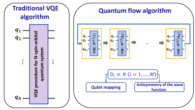
Figure 1: A schematic representation of the quantum flow algorithm. In this algorithm, the computational problem for a large space is translated into the computational flow involving coupled eigenvalue problems involving Hermitian $H^{\rm eff}(\mathfrak{h}_{i})\;(i=1,\ldots,M)$ (see text for more details)

V Multi-component CC downfolding

The development of computational algorithms for composite quantum systems keeps attracting a lot of attention in the field of quantum computing. Typical examples are related to quantum electrodynamics, nuclear physics, and quantum chemistry. In quantum chemistry, this effort is related to the development of methods for non-perturbative coupling of electronic degrees of freedom with strong external fields Haugland et al. (2020b); Pavošević and Flick (2021) and formulations going beyond Born-Oppenheimer approximation.Nakai and Sodeyama (2003); Ellis, Aggarwal, and Chakraborty (2016); Pavošević, Culpitt, and Hammes-Schiffer (2018); Pavošević and Hammes-Schiffer (2021) Given the current status of quantum computing technology, it is important to provide techniques for compressing the dimensionality of these problems or finding an effective potential experienced by the one type of particles.

For simplicity, in this section we will consider a fictitious system composed of two types of Fermions A and B, defined by two sets of creation/annihilation operators $\{a_{\alpha},a_{\alpha}^{\dagger}\}_{\alpha=1}^{N_{A}}$ and $\{b_{\beta},b_{\beta}^{\dagger}\}_{\beta=1}^{N_{B}}$ (these operators should not be confused with the notation used in Section II) satisfying typical Fermionic anti-commutation relations ($[.,.]_{+}$) and commuting ($[.,.]_{-}$) between themselves

$$[a_{\alpha},b_{\beta}]_{-}=[a_{\alpha},b^{\dagger}_{\beta}]_{-}=0\;,$$ (27)

$$[a^{\dagger}_{\alpha},b_{\beta}]_{-}=[a^{\dagger}_{\alpha},b^{\dagger}_{\beta}]_{-}=0\;.$$ (28)

We will also assume specific form of the Hamiltonian

$$H_{AB}=H_{A}+H_{B}+V_{AB}$$ (29)

where $H_{A}$, $H_{B}$, and $V_{AB}$ describe sub-systems A, B, and interactions between A and B, respectively. We will also assume that the interaction part commutes with the particle number operators $n_{A}$ and $n_{B}$ for systems A and B, i.e.,

$$[V_{AB},n_{A}]_{-}=[V_{AB},n_{B}]_{-}=0\;,$$ (30)

$$n_{A}=\sum_{\alpha=1}^{N_{A}}a^{\dagger}_{\alpha}a_{\alpha}\;\;,\;\;n_{B}=\sum_{\beta=1}^{N_{B}}b^{\dagger}_{\beta}b_{\beta}\;.$$ (31)

This situation is typically encountered in models relevant to non-Born-Oppenheimer approaches in electronic structure theory Nakai and Sodeyama (2003); Ellis, Aggarwal, and Chakraborty (2016); Pavošević, Culpitt, and Hammes-Schiffer (2018); Pavošević and Hammes-Schiffer (2021) and nuclear structure theory.Dean and Hjorth-Jensen (2004)

Let us assume that the correlated ground-state wave function can be represented in the form of single reference CC wave function

$$|\Psi_{AB}\rangle=e^{T_{AB}}|\Phi_{AB}\rangle\;,$$ (32)

where cluster operator contains excitations correlating sub-system A ($T_{A}$) and sub-system B ($T_{B}$) as well as collective excitations involving both sub-systems ($S_{AB}$), .i.e.,

$$T_{AB}=T_{A}+T_{B}+S_{AB}\;.$$ (33)

The reference function $|\Phi_{AB}\rangle$ is a reference function for the composite system which is assume to be represented as

$$|\Phi_{AB}\rangle=\Omega_{A}\Omega_{B}|0\rangle\;,$$ (34)

where $|0\rangle$ represents physical vacuum and $\Omega_{A}$ and $\Omega_{B}$ are string of $a^{\dagger}_{\alpha}$/$b^{\dagger}_{\beta}$ operators distributing electrons among occupied levels of sub-systems A and B, respectively.

The energy-dependent CC equation for the composite system takes the form

$$(P_{AB}+Q_{AB})H_{AB}e^{T_{AB}}|\Phi_{AB}\rangle=E_{AB}e^{T_{AB}}|\Phi_{AB}\rangle\;,$$ (35)

where $E_{AB}$ is the energy of the composite system, $P_{AB}$ is a projection operator onto the reference function $|\Phi_{AB}\rangle$, and projection operator $Q_{AB}$ can be decomposed as follows:

$$Q_{AB}=Q_{A}+Q_{B}+Z_{AB}\;,$$ (36)

where $Q_{A}$ and $Q_{B}$ are the projection operators onto excited Slater determinants obtained by exciting particles within sub-system A and B from $|\Phi_{AB}\rangle$, respectively, and $Z_{AB}$ corresponds to the projection operator onto sub-space spanned by excited Slater determinants where fermion particles of type A and B are excited simultaneously.

By projecting Eq. (35) onto $(P_{AB}+Q_{A})$ and introducing the resolution of identity $e^{T_{B}+S_{AB}}e^{-T_{B}-S_{AB}}$ one obtains

$$(P_{AB}+Q_{A})e^{T_{B}+S_{AB}}(\bar{H}_{AB,{\rm ext}}-E_{AB})e^{T_{A}}|\Phi_{AB}\rangle=0\;,$$ (37)

where

$$\bar{H}_{AB,{\rm ext}}=e^{-T_{B}-S_{AB}}H_{AB}e^{T_{B}+S_{AB}}\;.$$ (38)

In analogy to analysis in Ref. Kowalski, 2018 the role of $e^{T_{B}+S_{AB}}$ in Eq. (37), reduces to the unit operator. This is a consequence of the fact that the operator $T_{B}+S_{AB}$ produces excitations within sub-system B, which are subsequently eliminated by the $Q_{A}$ projection operator. Consequently, Eq. (37) takes the form:

$$H^{\rm eff}(A)e^{T_{A}}|\Phi_{AB}\rangle=E_{AB}e^{T_{A}}|\Phi_{AB}\rangle\;,$$ (39)

where the downfolded/effective Hamiltonian $H^{\rm eff}(A)$ is defined as

$$H^{\rm eff}(A)=(P_{AB}+Q_{A})\bar{H}_{AB,{\rm ext}}(P_{AB}+Q_{A})\;.$$ (40)

The above result shows that once $T_{B}$ and $S_{AB}$ amplitudes are know (or can be effectively approximated) the energy of the entire system can be calculated performing simulations on the sub-system A using effective Hamiltonian $H^{\rm eff}(A)$.

In addition to the simplest downfolding procedure described above, there are several other possible scenarios how downfolding procedures can be defined for the composite system:

• the utilization of second downfolding procedure to the $H^{\rm eff}(A)$ in reduced-size active space for sub-system A,

• the utilizaton of the composite active space that is representd by tensor product of active spaces for sub-systems A and B.

These techniques are especially interesting for the the explicit inclusion of nuclear degrees of freedom (for Fermionic nuclei) in the effective Hamiltonians describing electronic degrees of freedom in the non-Born-Oppenheimer formulations.

A Hermitian extension of the downfolding procedure can be accomplished by utilizing DUCC Ansatz for the composite system given by the expansion

$$|\Psi_{AB}\rangle=e^{\sigma_{B}+\rho_{AB}}e^{\sigma_{A}}|\Phi_{AB}\rangle\;,$$ (41)

where $\sigma_{A}$, $\sigma_{B}$, and $\rho_{AB}$ are the anti-Hermitian operators defined by the cluster amplitudes with indices belonging to sub-systems A, B, and amplitudes defined by a mixed indices involving basis functions on A and B, respectively. As in the non-Hermitian case of downfolding discussed in this Section, we will focus on the downfolding of the entire sub-system B into the effective Hamiltonians for sub-system A. Since creation/annihilation operators correspond to the sub-systems A and B, the exactness of the above expansion can be obtained as a generalization of the procedure based on the elementary Givens rotations discussed in Ref. Evangelista, Chan, and Scuseria, 2019. For the specific case discussed in this Section (based on the downfolding of the entire B sub-system) one should assume that all basis functions defining sub-system A are defined as active indices (see Ref.Kowalski and Bauman (2020) for details).

Substituting Eq. (41) into the Schrödinger equations and projecting onto $(P_{AB}+Q_{A})$, one arrives the following form of the equations

$$H^{\rm eff}_{DUCC}(A)e^{\sigma_{A}}|\Phi_{AB}\rangle=E_{AB}e^{\sigma_{A}}|\Phi_{AB}\rangle\;,$$ (42)

where

$$H^{\rm eff}_{DUCC}(A)=(P_{AB}+Q_{A})\bar{H}_{AB,{\rm ext}}(P_{AB}+Q_{A})\;,$$ (43)

and

$$\bar{H}_{AB,{\rm ext}}=e^{-\sigma_{B}-\rho_{AB}}He^{\sigma_{B}+\rho_{AB}}\;.$$ (44)

Again, the energy of the full system can be probed by sub-system A using effective Hamiltonian $H^{\rm eff}_{DUCC}(A)$. For example, one can envision the utilization of Eq. (42) in the context of coupling nuclear and electronic degrees of freedom. In this case, sub-system A is represented by electrons while system B corresponds do nuclei obeying Fermi statistic. If $\sigma_{B}$ and $\rho_{AB}$ can be effectively approximated then the $H^{\rm eff}_{DUCC}(A)$ Hamiltonian describes the behavior of electron in the presence of ”correlated” nuclei. The intensive development of the CC models beyond Born-Oppenheimer approximations Nakai and Sodeyama (2003); Pavošević, Culpitt, and Hammes-Schiffer (2018); Pavošević and Hammes-Schiffer (2021) provides a reference for building approximate, for eaxmple, perturbative, form of $\sigma_{B}$ and $\rho_{AB}$ according formula analogous to Eqs. (24), which requires the knowledge of $T_{B}$ and $S_{AB}$ to determine $\sigma_{B}$ and $\rho_{AB}$, respectively.

VI Extraction of the analytical form of interactions in many-body systems

In standard formulations of downfolding methods it is assumed (see Refs. Bauman et al., 2019; Metcalf et al., 2020)) that downfolded Hamiltonians are dominated by one- and two-body effects, i.e., using the language of second quantization $H^{\rm eff}$ can be approximated as (for simplicity, let us assume that only virtual orbitals are downfolded)

$$H^{\rm eff}_{DUCC}\simeq\sum_{PQ}\chi^{P}_{Q}a_{Q}^{\dagger}a_{P}+\frac{1}{2}\sum_{P,Q,R,S}\chi^{PQ}_{RS}a_{R}^{\dagger}a_{S}^{\dagger}a_{Q}a_{P}\;,$$ (45)

where $P,Q,R,S$ indices, $\chi^{P}_{Q}$, and $\chi^{PQ}_{RS}$ represent active spin orbitals and effective one- and two-body interactions, respectively (non-antisymmetrized matrix elements $\chi^{PQ}_{RS}$ are employed in (45)). Once the set of $\{\chi^{P}_{Q},\chi^{PQ}_{RS}\}$ is known (at the end of flow procedure) this information can be further used to derive an analytical form of effective inter-electron interactions. This can be accomplished by fitting the general form of one-body $u$ and two-body $g$ interactions defined as functions of to-be-optimized parameters ${\bm{\gamma}}$/${\bm{\delta}}$ as well as $r_{1}$, $r_{2}$, $r_{12}=|r_{1}-r_{2}|$, $\nabla_{1}$, $\nabla_{2}$, etc. operators:

$$u = u({\bm{\gamma}},r_{1},\nabla_{1},\ldots)\;,$$ (46)

$$g = g({\bm{\delta}},r_{1},r_{2},r_{12},\nabla_{1},\nabla_{2},\ldots)\;,$$ (47)

These effective interactions replace standard one- and two-body interactions in non-relativistic quantum chemistry and are defined to minimize the discrepancies with $\{\chi^{P}_{Q},\chi^{PQ}_{RS}\}$ for a given discrete molecular spin-orbital set, i.e.,

$$\min_{\bm{\gamma}}\{\sum_{PQ}|u^{P}_{Q}({\bm{\gamma}})-\chi^{P}_{Q}|\} \;,$$ (48)

$$\min_{\bm{\delta}}\{\sum_{PQRS}|g^{PQ}_{RS}({\bm{\delta}})-\chi^{PQ}_{RS}|\} \;,\;$$ (49)

where

$$u^{P}_{Q}({\bm{\gamma}}) = \int dx_{1}\phi_{Q}(x_{1})^{*}u({\bm{\gamma}},r_{1},\nabla_{1},\ldots)\phi_{P}(x_{1})\;,$$ (50)

$$g^{PQ}_{RS}({\bm{\delta}}) = \int dx_{1}dx_{2}\phi_{R}(x_{1})^{*}\phi_{S}(x_{2})^{*}g({\bm{\delta}},r_{1},r_{2},r_{12},\nabla_{1},\nabla_{2},\ldots)\phi_{P}(x_{1})\phi_{Q}(x_{2})\;.$$ (51)

We believe that the utilization of efficient non-linear optimizers or machine learning techniques can provide an effective form of the interactions $u$ and $g$ defined in small-size active spaces. These effective interactions can be utilized in low-order methodologies, including Hartree-Fock (HF) and density functional theories (DFT). In the latter case functions $u$ and $g$ can be utilized to develop/verify new forms of exchange-correlations functionals. The access to the analytical form of the inter-electron interactions can also enable affordable and reliable ab-initio dynamics driven by low-order methods.

VII Conclusions

In this paper, we briefly review the current state of two variants of CC downfolding techniques. While the non-Hermitian downfolding and resulting active-space Hamiltonians are not a primary target for quantum computing, the equivalence theorem opens new possibilities regarding forming systematic reduced-scaling frameworks based on the quantum flow equations. In contrast to the existing reduced scaling CC formulations, where the notion of electron pair is rather descriptive and is based on the partitioning of the correlation energy with respect to contributions that can be indexed by pairs of the occupied orbitals, the present formalism defines the pair through the corresponding effective Hamiltonian. This fact has a fundamental advantage over ad hoc localization procedures - it allows in a natural way to introduce the pair density matrix. It also allows for a more systematic way of introducing certain classes of higher-rank excitations. The double unitary CC Ansatz provides a natural many-body language to introduce Hermitian downfolded representation of many-body Hamiltonians in reduced-dimensionality active spaces. To approximate non-terminating commutator expansion of downfolded Hamiltonians, we use finite commutator expansions. On the LiF example, we demonstrated that the inclusion of double commutator terms leads to systematic improvements of the results obtained with single commutator expansion even in a situation when an active space is not providing a good zero-th order approximation of correlation effects. It should be also stressed that the downfolded Hamiltonians based on the double commutator expansion are capable of reducing the error of energies obtained by the diagonalization of the bare-Hamiltonian in the same-size active space by more than an order of magnitude (in fact, for the 1.0R_e and 5.0R_e one could witness 30- and 60-fold reduction in energy errors with respect to accurate CC results obtained by correlating all molecular orbitals).

In the second part of the paper, we extended non-Hermitian and Hermitian downfolding to multi-component quantum systems. As an example, we used the model system composed of two types of Fermions, which epitomize typical situations encountered in nuclear physics and for certain types of nuclei in non-Born-Oppenheimer electronic structure theory. We have also outlined an approximate procedure to extract the semi-analytical form of the one- and two-body inter-electron interactions in active space based on the minimization procedure utilizing one- and two-body interactions defining downfolded Hamiltonians. In the future, we will explore the usefulness of machine learning techniques for this procedure.

VIII Acknowledgement

This work was supported by the ”Embedding QC into Many-body Frameworks for Strongly Correlated Molecular and Materials Systems” project, which is funded by the U.S. Department of Energy, Office of Science, Office of Basic Energy Sciences (BES), the Division of Chemical Sciences, Geosciences, and Biosciences. Part of this work was supported by the Quantum Science Center (QSC), a National Quantum Information Science Research Center of the U.S. Department of Energy (DOE).

References

- Coester (1958) F. Coester, Nucl. Phys. 7, 421 (1958).
- Coester and Kummel (1960) F. Coester and H. Kummel, Nucl. Phys. 17, 477 (1960).
- Čížek (1966) J. Čížek, J. Chem. Phys. 45, 4256 (1966).
- Paldus, Čížek, and Shavitt (1972) J. Paldus, J. Čížek, and I. Shavitt, Phys. Rev. A 5, 50 (1972).
- Purvis and Bartlett (1982) G. Purvis and R. Bartlett, J. Chem. Phys. 76, 1910 (1982).
- Koch and Jørgensen (1990) H. Koch and P. Jørgensen, J. Chem. Phys. 93, 3333 (1990).
- Paldus and Li (1999) J. Paldus and X. Li, Adv. Chem. Phys. 110, 1 (1999).
- Crawford and Schaefer (2000) T. D. Crawford and H. F. Schaefer, Reviews in computational chemistry 14, 33 (2000).
- Bartlett and Musiał (2007) R. J. Bartlett and M. Musiał, Rev. Mod. Phys. 79, 291 (2007).
- Funke, Kaulfuss, and Kümmel (1987) M. Funke, U. Kaulfuss, and H. Kümmel, Physical Review D 35, 621 (1987).
- Kümmel (2001) H. G. Kümmel, Physical Review B 64, 014301 (2001).
- Hasberg and Kümmel (1986) G. Hasberg and H. Kümmel, Physical Review C 33, 1367 (1986).
- Bishop, Ligterink, and Walet (2006) R. F. Bishop, N. Ligterink, and N. R. Walet, International journal of modern physics B 20, 4992 (2006).
- Ligterink, Walet, and Bishop (1998) N. Ligterink, N. Walet, and R. Bishop, Annals of Physics 267, 97 (1998).
- Arponen et al. (1988) J. Arponen, R. Bishop, E. Pajanne, and N. Robinson, in Condensed matter theories (Springer, 1988) pp. 51–66.
- Bishop et al. (1989) R. Bishop, N. Robinson, J. Arponen, and E. Pajanne, in Aspects of Many-Body Effects in Molecules and Extended Systems (Springer, 1989) pp. 241–260.
- Dean and Hjorth-Jensen (2004) D. J. Dean and M. Hjorth-Jensen, Phys. Rev. C 69, 054320 (2004).
- Kowalski et al. (2004) K. Kowalski, D. J. Dean, M. Hjorth-Jensen, T. Papenbrock, and P. Piecuch, Phys. Rev. Lett. 92, 132501 (2004).
- Hagen et al. (2008) G. Hagen, T. Papenbrock, D. J. Dean, and M. Hjorth-Jensen, Phys. Rev. Lett. 101, 092502 (2008).
- Scheiner et al. (1987) A. C. Scheiner, G. E. Scuseria, J. E. Rice, T. J. Lee, and H. F. Schaefer III, The Journal of chemical physics 87, 5361 (1987).
- Sinnokrot, Valeev, and Sherrill (2002) M. O. Sinnokrot, E. F. Valeev, and C. D. Sherrill, Journal of the American Chemical Society 124, 10887 (2002).
- Slipchenko and Krylov (2002) L. V. Slipchenko and A. I. Krylov, The Journal of chemical physics 117, 4694 (2002).
- Tajti et al. (2004) A. Tajti, P. G. Szalay, A. G. Császár, M. Kállay, J. Gauss, E. F. Valeev, B. A. Flowers, J. Vázquez, and J. F. Stanton, The Journal of chemical physics 121, 11599 (2004).
- Crawford (2006) T. D. Crawford, Theoretical Chemistry Accounts 115, 227 (2006).
- Parkhill, Lawler, and Head-Gordon (2009) J. A. Parkhill, K. Lawler, and M. Head-Gordon, The Journal of chemical physics 130, 084101 (2009).
- Riplinger and Neese (2013) C. Riplinger and F. Neese, The Journal of chemical physics 138, 034106 (2013).
- Yuwono, Magoulas, and Piecuch (2020) S. H. Yuwono, I. Magoulas, and P. Piecuch, Science Advances 6, eaay4058 (2020).
- Stoll (1992) H. Stoll, Physical Review B 46, 6700 (1992).
- Hirata et al. (2004a) S. Hirata, R. Podeszwa, M. Tobita, and R. J. Bartlett, J. Chem. Phys. 120, 2581 (2004a).
- Katagiri (2005) H. Katagiri, The Journal of chemical physics 122, 224901 (2005).
- Booth et al. (2013) G. H. Booth, A. Grüneis, G. Kresse, and A. Alavi, Nature 493, 365 (2013).
- Degroote et al. (2016) M. Degroote, T. M. Henderson, J. Zhao, J. Dukelsky, and G. E. Scuseria, Physical Review B 93, 125124 (2016).
- McClain et al. (2017) J. McClain, Q. Sun, G. K.-L. Chan, and T. C. Berkelbach, Journal of chemical theory and computation 13, 1209 (2017).
- Wang and Berkelbach (2020) X. Wang and T. C. Berkelbach, Journal of Chemical Theory and Computation 16, 3095 (2020).
- Haugland et al. (2020a) T. S. Haugland, E. Ronca, E. F. Kjønstad, A. Rubio, and H. Koch, Phys. Rev. X 10, 041043 (2020a).
- Brandow (1967) B. H. Brandow, Rev. Mod. Phys. 39, 771 (1967).
- Lindgren and Morrison (2012) I. Lindgren and J. Morrison, Atomic Many-Body Theory, Springer Series on Atomic, Optical, and Plasma Physics (Springer Berlin Heidelberg, 2012).
- Shavitt and Bartlett (2009) I. Shavitt and R. Bartlett, Many-Body Methods in Chemistry and Physics: MBPT and Coupled-Cluster Theory, Cambridge Molecular Science (Cambridge University Press, 2009).
- Raghavachari et al. (1989) K. Raghavachari, G. W. Trucks, J. A. Pople, and M. Head-Gordon, Chem. Phys. Lett. 157, 479 (1989).
- Piecuch and Kowalski (2011) P. Piecuch and K. Kowalski, “In search of the relationship between multiple solutions characterizing coupled-cluster theories,” in Computational Chemistry: Reviews of Current Trends (WORLD SCIENTIFIC, 2011) pp. 1–104.
- Kowalski and Piecuch (2000a) K. Kowalski and P. Piecuch, J. Chem. Phys. 113, 18 (2000a).
- Kowalski and Piecuch (2000b) K. Kowalski and P. Piecuch, J. Chem. Phys. 113, 5644 (2000b).
- Piecuch and Włoch (2005) P. Piecuch and M. Włoch, J. Chem. Phys. 123, 224105 (2005).
- Cramer et al. (2006) C. J. Cramer, A. Kinal, M. Włoch, P. Piecuch, and L. Gagliardi, J. Phys. Chem. A 110, 11557 (2006).
- Włoch, Gour, and Piecuch (2007) M. Włoch, J. R. Gour, and P. Piecuch, J. Phys. Chem. A 111, 11359 (2007).
- Piecuch, Gour, and Włoch (2009) P. Piecuch, J. R. Gour, and M. Włoch, Int. J. Quantum Chem. 109, 3268 (2009).
- Deustua, Shen, and Piecuch (2017) J. E. Deustua, J. Shen, and P. Piecuch, Physical review letters 119, 223003 (2017).
- Deustua et al. (2018) J. E. Deustua, I. Magoulas, J. Shen, and P. Piecuch, The Journal of Chemical Physics 149, 151101 (2018).
- Bauman, Shen, and Piecuch (2017) N. P. Bauman, J. Shen, and P. Piecuch, Mol. Phys. 115, 2860 (2017).
- Stanton (1997) J. F. Stanton, Chem. Phys. Lett. 281, 130 (1997).
- Stanton and Gauss (1995) J. F. Stanton and J. Gauss, J. Chem. Phys. 103, 1064 (1995).
- Crawford and Stanton (1998) T. D. Crawford and J. F. Stanton, Int. J. Quantum Chem. 70, 601 (1998).
- Kucharski and Bartlett (1998a) S. A. Kucharski and R. J. Bartlett, J. Chem. Phys. 108, 5243 (1998a).
- Kucharski and Bartlett (1998b) S. A. Kucharski and R. J. Bartlett, J. Chem. Phys. 108, 5255 (1998b).
- Gwaltney and Head-Gordon (2000) S. R. Gwaltney and M. Head-Gordon, Chem. Phys. Lett. 323, 21 (2000).
- Gwaltney and Head-Gordon (2001) S. R. Gwaltney and M. Head-Gordon, J. Chem. Phys. 115, 2014 (2001).
- Hirata et al. (2001) S. Hirata, M. Nooijen, I. Grabowski, and R. J. Bartlett, J. Chem. Phys. 114, 3919 (2001).
- Bomble et al. (2005) Y. J. Bomble, J. F. Stanton, M. Kallay, and J. Gauss, J. Chem. Phys. 123, 054101 (2005).
- Kucharski and Bartlett (1998c) S. A. Kucharski and R. J. Bartlett, J. Chem. Phys. 108, 9221 (1998c).
- Meissner and Bartlett (2001) L. Meissner and R. J. Bartlett, J. Chem. Phys. 115, 50 (2001).
- Robinson and Knowles (2013) J. B. Robinson and P. J. Knowles, J. Chem. Phys. 138, 074104 (2013).
- Bozkaya and Schaefer III (2012) U. Bozkaya and H. F. Schaefer III, J. Chem. Phys. 136, 204114 (2012).
- Hampel and Werner (1996) C. Hampel and H.-J. Werner, The Journal of chemical physics 104, 6286 (1996).
- Schütz (2000) M. Schütz, The Journal of Chemical Physics 113, 9986 (2000).
- Schütz and Werner (2000) M. Schütz and H.-J. Werner, Chemical Physics Letters 318, 370 (2000).
- Schütz and Werner (2001) M. Schütz and H.-J. Werner, The Journal of Chemical Physics 114, 661 (2001).
- Li, Ma, and Jiang (2002) S. Li, J. Ma, and Y. Jiang, J. Comp. Chem. 23, 237 (2002).
- Li et al. (2006) S. Li, J. Shen, W. Li, and Y. Jiang, J. Chem. Phys. 125, 074109 (2006).
- Li et al. (2009) W. Li, P. Piecuch, J. R. Gour, and S. Li, J. Chem. Phys. 131, 114109 (2009).
- Li and Piecuch (2010) W. Li and P. Piecuch, J. Phys. Chem. A 114, 6721 (2010).
- Neese, Wennmohs, and Hansen (2009) F. Neese, F. Wennmohs, and A. Hansen, The Journal of chemical physics 130, 114108 (2009).
- Neese et al. (2009) F. Neese, A. Hansen, F. Wennmohs, and S. Grimme, Accounts of chemical research 42, 641 (2009).
- Riplinger et al. (2016) C. Riplinger, P. Pinski, U. Becker, E. F. Valeev, and F. Neese, J. Chem. Phys. 144, 024109 (2016).
- Riplinger et al. (2013) C. Riplinger, B. Sandhoefer, A. Hansen, and F. Neese, The Journal of Chemical Physics 139, 134101 (2013).
- Pavosevic et al. (2016) F. Pavosevic, P. Pinski, C. Riplinger, F. Neese, and E. F. Valeev, Journal of Chemical Physics 144 (2016), 10.1063/1.4945444.
- D’Cunha and Crawford (2020) R. D’Cunha and T. D. Crawford, Journal of Chemical Theory and Computation 17, 290 (2020).
- Dutta, Neese, and Izsák (2016) A. K. Dutta, F. Neese, and R. Izsák, The Journal of chemical physics 144, 034102 (2016).
- Peng, Clement, and Valeev (2018) C. Peng, M. C. Clement, and E. F. Valeev, Journal of chemical theory and computation 14, 5597 (2018).
- Kowalski (2018) K. Kowalski, J. Chem. Phys. 148, 094104 (2018).
- Kowalski (2021) K. Kowalski, Phys. Rev. A 104, 032804 (2021).
- Kowalski and Bauman (2020) K. Kowalski and N. P. Bauman, The Journal of Chemical Physics 152, 244127 (2020), https://doi.org/10.1063/5.0008436 .
- Bauman et al. (2019) N. P. Bauman, E. J. Bylaska, S. Krishnamoorthy, G. H. Low, N. Wiebe, C. E. Granade, M. Roetteler, M. Troyer, and K. Kowalski, J. Chem. Phys. 151, 014107 (2019).
- Bauman, Low, and Kowalski (2019) N. P. Bauman, G. H. Low, and K. Kowalski, The Journal of Chemical Physics 151, 234114 (2019).
- Bauman et al. (2020) N. P. Bauman, J. Chládek, L. Veis, J. Pittner, and K. Kowalski, arXiv preprint arXiv:2011.01985 (2020).
- Peruzzo et al. (2014) A. Peruzzo, J. McClean, P. Shadbolt, M.-H. Yung, X.-Q. Zhou, P. J. Love, A. Aspuru-Guzik, and J. L. O’brien, Nat. Commun. 5, 4213 (2014).
- McClean et al. (2016) J. R. McClean, J. Romero, R. Babbush, and A. Aspuru-Guzik, New J. Phys 18, 023023 (2016).
- Romero et al. (2018) J. Romero, R. Babbush, J. R. McClean, C. Hempel, P. J. Love, and A. Aspuru-Guzik, Quantum Sci. Technol. 4, 014008 (2018).
- Shen et al. (2017) Y. Shen, X. Zhang, S. Zhang, J.-N. Zhang, M.-H. Yung, and K. Kim, Phys. Rev. A 95, 020501 (2017).
- Kandala et al. (2017) A. Kandala, A. Mezzacapo, K. Temme, M. Takita, M. Brink, J. M. Chow, and J. M. Gambetta, Nature 549, 242 (2017).
- Kandala et al. (2019) A. Kandala, K. Temme, A. D. Corcoles, A. Mezzacapo, J. M. Chow, and J. M. Gambetta, Nature 567, 491 (2019).
- Colless et al. (2018) J. I. Colless, V. V. Ramasesh, D. Dahlen, M. S. Blok, M. E. Kimchi-Schwartz, J. R. McClean, J. Carter, W. A. de Jong, and I. Siddiqi, Phys. Rev. X 8, 011021 (2018).
- Huggins et al. (2020) W. J. Huggins, J. Lee, U. Baek, B. O’Gorman, and K. B. Whaley, New Journal of Physics 22, 073009 (2020).
- Cao et al. (2019) Y. Cao, J. Romero, J. P. Olson, M. Degroote, P. D. Johnson, M. Kieferová, I. D. Kivlichan, T. Menke, B. Peropadre, N. P. Sawaya, et al., Chemical reviews 119, 10856 (2019).
- Kitaev (1997) A. Y. Kitaev, Russian Mathematical Surveys 52, 1191 (1997).
- Nielsen and Chuang (2011) M. A. Nielsen and I. L. Chuang, Quantum Computation and Quantum Information: 10th Anniversary Edition, 10th ed. (Cambridge University Press, New York, NY, USA, 2011).
- Luis and Peřina (1996) A. Luis and J. Peřina, Phys. Rev. A 54, 4564 (1996).
- Cleve et al. (1998) R. Cleve, A. Ekert, C. Macchiavello, and M. Mosca, Proc. R. Soc. Lond. A 454, 339 (1998).
- Berry et al. (2007) D. W. Berry, G. Ahokas, R. Cleve, and B. C. Sanders, Comm. Math. Phys. 270, 359 (2007).
- Childs (2010) A. M. Childs, Comm. Math. Phys. 294, 581 (2010).
- Seeley, Richard, and Love (2012) J. T. Seeley, M. J. Richard, and P. J. Love, J. Chem. Phys. 137, 224109 (2012).
- Wecker, Hastings, and Troyer (2015) D. Wecker, M. B. Hastings, and M. Troyer, Phys. Rev. A 92, 042303 (2015).
- Häner et al. (2016) T. Häner, D. S. Steiger, M. Smelyanskiy, and M. Troyer, in SC ’16: Proceedings of the International Conference for High Performance Computing, Networking, Storage and Analysis (2016) pp. 866–874.
- Poulin et al. (2017) D. Poulin, A. Kitaev, D. S. Steiger, M. B. Hastings, and M. Troyer, arXiv preprint arXiv:1711.11025 (2017).
- Dunning Jr. (1989) T. H. Dunning Jr., J. Chem. Phys. 90, 1007 (1989).
- Hirata et al. (2004b) S. Hirata, P.-D. Fan, A. A. Auer, M. Nooijen, and P. Piecuch, The Journal of chemical physics 121, 12197 (2004b).
- Haugland et al. (2020b) T. S. Haugland, E. Ronca, E. F. Kjønstad, A. Rubio, and H. Koch, Physical Review X 10, 041043 (2020b).
- Pavošević and Flick (2021) F. Pavošević and J. Flick, arXiv preprint arXiv:2106.09842 (2021).
- Nakai and Sodeyama (2003) H. Nakai and K. Sodeyama, The Journal of chemical physics 118, 1119 (2003).
- Ellis, Aggarwal, and Chakraborty (2016) B. H. Ellis, S. Aggarwal, and A. Chakraborty, Journal of chemical theory and computation 12, 188 (2016).
- Pavošević, Culpitt, and Hammes-Schiffer (2018) F. Pavošević, T. Culpitt, and S. Hammes-Schiffer, Journal of chemical theory and computation 15, 338 (2018).
- Pavošević and Hammes-Schiffer (2021) F. Pavošević and S. Hammes-Schiffer, Journal of Chemical Theory and Computation 17, 3252 (2021).
- Evangelista, Chan, and Scuseria (2019) F. A. Evangelista, G. K.-L. Chan, and G. E. Scuseria, The Journal of Chemical Physics 151, 244112 (2019).
- Metcalf et al. (2020) M. Metcalf, N. P. Bauman, K. Kowalski, and W. A. de Jong, Journal of Chemical Theory and Computation 16, 6165 (2020), pMID: 32915568, https://doi.org/10.1021/acs.jctc.0c00421 .