Learning Model Predictive Controllers for Real-Time Ride-Hailing Vehicle Relocation and Pricing Decisions

Abstract

Large-scale ride-hailing systems often combine real-time routing at the individual request level with a macroscopic Model Predictive Control (MPC) optimization for dynamic pricing and vehicle relocation. The MPC relies on a demand forecast and optimizes over a longer time horizon to compensate for the myopic nature of the routing optimization. However, the longer horizon increases computational complexity and forces the MPC to operate at coarser spatial-temporal granularity, degrading the quality of its decisions. This paper addresses these computational challenges by learning the MPC optimization. The resulting machine-learning model then serves as the optimization proxy and predicts its optimal solutions. This makes it possible to use the MPC at higher spatial-temporal fidelity, since the optimizations can be solved and learned offline. Experimental results show that the proposed approach improves quality of service on challenging instances from the New York City dataset.

1 Introduction

The rapid growth of ride-hailing markets has transformed urban mobility, offering on-demand mobility services via mobile applications. While major ride-hailing platforms such as Uber and Didi leverage centralized dispatching algorithms to find good matching between drivers and riders, operational challenges persist due to imbalance between demand and supply. Consider morning rush hours as an example: most trips originate from residential areas to business districts where a large number of vehicles accumulate and remain idle. Relocating these vehicles back to the demand area is thus crucial to maintaining quality of service and income for the drivers. In cases where demand significantly exceeds supply, dynamic pricing is needed to ensure that demand does not surpass service capacity.

Extensive studies have focused on real-time vehicle relocation and pricing problems. Existing methodologies fit broadly into two categories: optimization-based approach and learning-based approach. Optimization-based approaches involve the solving of a mathematical program using expected demand and supply information over a future horizon. Learning-based approaches (predominantly reinforcement learning) train a state-based decision policy by interacting with the environment and observing the rewards. While both approaches have demonstrated promising performance in simulation and (in some cases) real-world deployment (Jiao et al. 2021), they have obvious drawbacks: the optimization needs to be solved in real-time and often trades off fidelity (hence quality of solutions) for computational efficiency. Reinforcement-learning approaches require a tremendous amount of data to explore high-dimensional state-action spaces and often simplify the problem to ensure efficient training. While a complex real-world system like ride-hailing may never admit a perfect solution, there are certainly possibilities for improvement.

This paper presents a step to overcoming these computational challenges. It considers large-scale ride-hailing systems with real-time routing for individual requests and a macroscopic Model Predictive Control (MPC) optimization for dynamic pricing and vehicle relocation. Its key idea is to replace the MPC optimization with a machine-learning model that serves as the optimization proxy and predicts the MPC’s optimal solutions. The proposed approach allows ride-hailing systems to consider the MPC at higher spatial or temporal fidelity since the optimizations can be solved and learned offline.

Learning the MPC however, comes with several challenges. First, the decisions are interdependent: where the vehicles should relocate depends on the demand which is governed by price. This imposes implicit correlation among the predictions, which are hard to enforce in classic regression models. Second, the predictions are of high dimensions (e.g., the number of vehicles to relocate between pairs of zones) and sparse, as relocations typically occur only between a few low-demand and high-demand regions. Capturing such patterns is difficult even with large amount of data. Third, the predicted solutions may not be feasible, as most prediction models cannot enforce the physical constraints that the solutions need to satisfy.

To solve these challenges, this paper proposes a sequential learning framework that first predicts the pricing decisions and then the relocation decisions based on the predicted prices. Furthermore, the framework utilizes an aggregation-disaggregation procedure that learns the decisions at an aggregated level to overcome the high dimensionality and sparsity, and then converts them back to feasible solutions on the original granularity by a polynomial-time solvable transportation optimization. As a consequence, during real-time operations, the original NP-Hard and computationally demanding MPC optimization is replaced by a polynomial-time problem of sequential prediction and optimization.

The proposed learning & optimization framework is evaluated on the New York Taxi data set and serves $6.7\%$ more riders than the original optimization approach due to its higher fidelity. The results suggest that a hybrid approach combining machine learning and tractable optimization may provide an appealing avenue for certain classes of real-time problems.

The paper is organized as follows. Section 2 summarizes the existing literature. Section 3 gives an overview of the considered real-time ride-hailing operations. Section 4 contains the main contributions and presents the learning framework. Section 5 reports the experimental results on a large-scale case study in New York City.

2 Related Work

While there have been abundant works on the theoretical side of relocation and pricing (most works model the ride-hailing market as a one-sided/two-sided market and study properties of different relocation/pricing policies at market equilibrium), this paper is interested in real-time pricing and relocation which is reviewed in this section.

Prior works on real-time pricing and/or relocation fit broadly into two frameworks: model predictive control (MPC) ((Miao et al. 2015; Zhang, Rossi, and Pavone 2016; Iglesias et al. 2017; Huang, de Almeida Correia, and An 2018; Riley, Van Hentenryck, and Yuan 2020) for relocation and (Ma, Fang, and Parkes 2019; Lei, Jiang, and Ouyang 2019) for pricing), and reinforcement learning (RL) ((Verma et al. 2017; Oda and Joe-Wong 2018; Guériau and Dusparic 2018; Lin et al. 2018; Jin et al. 2019; Jiao et al. 2021; Liang et al. 2021) for relocation and (Qiu, Li, and Zhao 2018; Lei, Jiang, and Ouyang 2019; Chen et al. 2019) for pricing). MPC is an online control procedure that repeatedly solves an optimization problem over a moving time window to find the best control action. System dynamics, i.e., the interplay between demand and supply, are explicitly modeled as mathematical constraints. Due to computational complexity, almost all the MPC models in the literature work at discrete spatial-temporal scale (dispatch area partitioned into zones, time into epochs) and use a relatively coarse granularity (a small number of zones or epochs).

Reinforcement learning, on the contrary, does not explicitly model system dynamics and trains a decision policy offline by approximating the state/state-action value function. It can be divided into two streams: single-agent RL and multi-agent RL. Single-agent RL focuses on maximizing reward of an individual agent, and multi-agent RL maximizes collective rewards of all the agents. The main challenge of this approach is to efficiently learn the state-action value function, which is high-dimensional (often infinite-dimensional) due to the complex and fast-changing demand-supply dynamics that arises in real-time settings. Since RL learns solely from interacting with the environment, a tremendous amount of samples need to be generated to fully explore the state-action space. Consequently, many works simplify the problem by using the same policy for agents within the same region (Verma et al. 2017; Lin et al. 2018), or restrict relocations to only neighboring regions (Oda and Joe-Wong 2018; Guériau and Dusparic 2018; Jin et al. 2019; Jiao et al. 2021). In addition, there is no guarantee on the performance of the policy when system dynamics deviates from the environment in which the policy is trained.

Our approach tries to combine the strength of both worlds - it models the system dynamics explicitly through a sophisticated MPC model, and approximates the optimal solutions of the MPC by machine learning to overcome the real-time computational challenges. As far as the authors know, the only work that has taken a similar approach is by Lei, Qian, and Ukkusuri (2020), which learns the decisions of a relocation model and show that the learned policy performs close to the original model. However, their model does not include pricing and considers only one epoch (10 mins). This paper focuses on a much more sophisticated MPC incorporating both relocation and pricing decisions and tracks how demand and supply interact over the course of multiple epochs. As a consequence, the model is significantly harder to learn since the solution space is exponentially larger. To tackle this challenge, this paper designs an aggregation-disaggregation learning framework and shows that the learned policy achieves superior performance than the original model due to its ability to use a finer granularity within the computational limits.

3 The Real-Time Ride-Hailing Operations

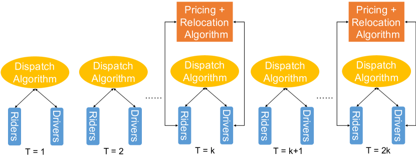
Figure 1: The Real-Time Ride-Hailing Operations.

This paper considers the real-time ride-hailing framework from Riley, Van Hentenryck, and Yuan (2020) (illustrated in Figure 1). The framework has two key components: a vehicle routing algorithm and an MPC component for idle vehicle relocation and pricing. The vehicle routing algorithm assigns riders to vehicles and chooses the vehicle routes. It operates at the individual request level with high frequency (e.g., every $30$ seconds). Because of the tight time constraints and the large number of requests, the routing algorithm is myopic, taking only the current demand into account. In contrast, the MPC component anticipates the demand and runs at a lower frequency (e.g., every $5-20$ minutes). The MPC component tackles the relocation and pricing decisions together as they are interdependent: relocation decisions depend on the demand, and the demand is shaped by the pricing decisions. The rest of this section reviews the two components.

3.1 The Routing Algorithm

The routing algorithm batches requests into a time window and optimizes every 30 seconds (Riley, Legrain, and Van Hentenryck 2019). Its objective is to minimize a weighted sum of passenger waiting times and penalties for unserved requests. Each time a request is not scheduled by the routing optimization, its penalty is increased in the next time window giving the request a higher priority. The routing algorithm is solved by column generation: it iterates between solving a restricted master problem (RMP), which assigns a route (sequence of pickups and dropoffs) to each vehicle, and a pricing subproblem, which generates feasible routes for the vehicles. The RMP is depicted in Figure 2. $R$ denotes the set of routes. $V$ the set of vehicles, and $P$ the set of passengers. $R_{v}$ denotes the subset of feasible routes for vehicle $v$. A route is feasible for a vehicle if it does not exceed the vehicle capacity and does not incur too much of a detour for its passengers due to ride-sharing. $c_{r}$ represents the wait times incurred by all customers served by route $r$. $p_{i}$ is the penalty of not scheduling request $i$, and $a_{i}^{r}=1$ iff request $i$ is served by route $r$. Decision variable $y_{r}\in[0,1]$ is 1 iff route $r$ is selected and $z_{i}\in[0,1]$ is 1 iff request $i$ is not served by any of the selected routes. The objective function minimizes the waiting times of the served customers and the penalties for the unserved customers. Constraints (2b) ensure that $z_{i}$ is set to 1 if request $i$ is not served by any of the selected routes and constraints (2c) ensure that only one route is selected per vehicle. The column generation process terminates when the pricing subproblem cannot generate new routes to improve the solution of the RMP or the solution time limit is met.

$$\min \quad\sum_{r\in R}c_{r}y_{r}+\sum_{i\in P}p_{i}z_{i}$$ (2a)

s.t. $$\left(\sum_{r\in R}y_{r}a_{i}^{r}\right)+z_{i}=1 \forall i\in P$$ (2b)

$$\sum_{r\in R_{v}}y_{r}=1 \forall v\in V$$ (2c)

$$z_{i}\in\mathbb{N} \forall i\in P$$ (2d)

$$y_{r}\in\{0,1\} \forall r\in R$$ (2e)

Figure 2: The Resricted Master Problem Formulation.

3.2 The MPC Component

The MPC follows a rolling time horizon approach that discretizes time into epochs of equal length and performs three tasks at each decision epoch: (1) it predicts the demand for the next $T$ epochs; (2) it optimizes relocation and pricing decisions over these epochs; and (3) it implements the decisions of the first epoch only. Due to the potentially large number of vehicles and riders in real-time, making pricing and relocation decisions for individual requests and vehicles is daunting computationally. For this reason, the MPC component operates at coarser temporal and spatial granularity: it partitions the geographical area into zones (not necessarily of equal size or shape) and considers pricing decisions at the zone level and relocation decisions at the zone-to-zone level. The MPC assumes that vehicles only pick up demand in the same zone and that vehicles, once they start delivering passengers or relocating, must finish their current trip before taking another assignment. These assumptions help the MPC model approximate the behavior of the underlying routing algorithm (but the routing algorithm does not have to obey these constraints). The only interactions between the routing optimization and the MPC components are the relocation decisions. To model reasonable waiting times, riders can only be picked up within $s$ epochs of their requests: they drop out if waiting more than $s$ epochs.

The impact of pricing on the demand is specified by the following process. Let $D^{0}_{ijt}$ denote the number of vehicles needed to serve expected riders from zone $i$ to zone $j$ under the baseline price (i.e., without surge pricing or promotion discount). At each epoch $t$, the MPC component determines the demand multiplier $\gamma_{it}$, where $\gamma_{it}\in[0,1]$ represents the proportion of demand to keep in the zone (e.g., $\gamma_{it}=0.8$ means 80% demand from zone $i$ will be kept and 20% will be priced out). The price corresponding to each demand multiplier can be estimated from historical market data and is taken as prior knowledge. The MPC assumes that a set of demand multipliers $\{\gamma^{k}_{it}\}_{k\in K}$ along with the corresponding demand $\{D^{k}_{ijt}\}_{k\in K}:=\{\gamma^{k}_{it}D^{0}_{ijt}\}_{k\in K}$ is available for each zone and epoch. The model aims at selecting the demand multipliers (and hence the demand) such that every rider is served in reasonable time.

Model Input
$V_{it}$	Number of vehicles that will become idle in $i$ during $t$
$\{D^{k}_{ijt}\}_{k\in K}$	Set of demand from $i$ to $j$ during $t$ available to be selected
$\lambda_{ij}$	Number of epochs to travel from $i$ to $j$
Model Parameters
$s$	Number of epochs that a rider remains in the system
$W_{ij}$	Average number of riders from $i$ to $j$ that a vehicle carries
$q^{p}(t,\rho)$	Weight of a rider served at $\rho$ whose request was placed at $t$
$q^{r}_{ij}(t)$	Relocation cost between $i$ and $j$ in $t$
Decision Variables
$p^{k}_{it}\in\{0,1\}$	Whether the $k$th demand multiplier $\gamma_{it}^{k}$ is chosen for zone $i$ and epoch $t$
$x_{ijt}^{r}\in\mathbb{Z}_{+}$	Number of vehicles starting to relocate from $i$ to $j$ during $t$
Auxiliary Variables
$v_{ijt}\in\mathbb{Z}_{+}$	Number of vehicles needed to serve all expected riders from $i$ to $j$ whose requests are placed at $t$
$x_{ijt\rho}^{p}\in\mathbb{Z}_{+}$	Number of vehicles that start to serve at time $\rho$ riders going from $i$ to $j$ whose requests were placed at $t$
$l_{it}\in\{0,1\}$	Whether there is unserved demand in $i$ at the end of epoch $t$

Table 1: The Nomenclature for the MPC Optimization.

[2]¡b¿ i,j∑t,ρ∑q^p(t,ρ) W_ijx^p_ijtρ - i,j∑t∑q^r_ij(t) x^r_ijt ∑_k∈K p^k_it=1 v_ijt=∑_k∈K D_ijt^k p^k_it   ∑_ρ∈ϕ(t) x^p_ijtρ = v_ijt        (t≤T-s+1) ∑_ρ∈ϕ(t) x^p_ijtρ ≤v_ijt        (t¿T-s+1) ∑_j,t_0 x^p_ijt_0 t + ∑_j x^r_ijt - V_i t = ∑_j,t_0 x^p_jit_0 (t - λ_ji) + ∑_j x^r_ji(t - λ_ji) ∑_j x^r_ijt≤M l_it ∑_j ∑_t_0:   t∈ϕ(t_0) (v_ijt - ∑_ρ=t_0^t x^p_ijt_0ρ ) ≤M(1 - l_it) x^p_ijtρ, x^r_ijt, v_ijt∈Z_+ p^k_it, l_it∈{0,1}

Figure 3: The MPC Optimization with Pricing & Relocation.

The MPC Formulation

The MPC optimization decides the zone pricing and the zone-to-zone relocation so that every rider is served in $s$ epochs. Table 1 summarizes its nomenclature and Figure 3 presents the optimization model. In the model, $i,j$ denote zones and $t_{0},t,\rho$ epochs. The ride-sharing coefficient $W_{ij}$ represents the average number of riders traveling from $i$ to $j$ that a vehicle carries accounting for ride-sharing. The time-dependent weights $q^{p}(t,\rho)$ and $q^{r}_{ij}(t)$ are designed to favor serving requests and performing relocations early, and to avoid postponing them: they are decreasing in $t$ and $\rho$.

The decision variables $p_{it}$ and $x^{r}_{ijt}$ capture the pricing and relocation decisions. Although decisions are made for each epoch in the time horizon, only the first epoch’s decisions are actionable and implemented: the next MPC execution will reconsider the decisions for subsequent epochs. Note that the auxiliary variables $x^{p}_{ijt\rho}$ are only defined for a subset of the subscripts, since riders drop out if they are not served in reasonable time. The valid subscripts for variables $x^{p}_{ijt\rho}$ must satisfy the constraint $1\leq t\leq\rho\leq\min(T,t+s-1)$. These conditions are implicit in the model for simplicity. Furthermore, $\phi(t)=\{\rho\in\mathcal{T}:t\leq\rho\leq t+s-1\}$ denotes the set of valid pick-up epochs for riders placing their requests in epoch $t$.

The MIP model maximizes the weighted sum of customers served and minimizes the relocation cost. Constraint (3) ensures that the model selects exactly one demand multiplier for each zone and epoch. Constraint (3) derives the number of vehicles needed to serve the demand from $i$ to $j$ whose requests are placed at $t$ as a function of the demand multiplier selected (captured by variable $p^{k}_{it}$). Constraint (3) enforces the service guarantees: it makes sure that riders with requests in the first $(T-s+1)$ epochs are served in the time horizon since they have at least $s$ epochs to be served. Constraint (3) makes sure that the served demand does not exceed the true demand. Constraint (3) is the flow balance constraint for each zone and epoch. Constraints (3) and (3) prevent vehicles from relocating unless all demand in the zone is served, approximating the behavior of the routing algorithm which favors scheduling vehicles to nearby requests. Constraints (3) - (3) specify the ranges of the variables. Constraint (3) - (3) are defined for all $(i,j,t)$, and (3) and (3) - (3) are defined for all $(i,t)$. The model is always feasible when the demand can be reduced to $0$ in all zones and epochs. The MIP model is challenging to solve at high fidelity when the number of zones $|Z|$, the length of time horizon $|\mathcal{T}|$, or the number of demand multipliers $|K|$ is large. This is the key motivation for learning the MPC optimization. By solving the MPC optimization offline and learning its optimal solutions, the MPC component would be able to operate at finer spatial and temporal granularity and make more informed decisions. This paper explores this avenue.

4 The Learning Methodology

The learning methodology approximates the MPC decisions in the first epoch since only these decisions are actionable after the MPC execution. Its architecture is depicted in Figure 4: it first learns the pricing decisions, which shape the demand, and then the relocation decisions. This section describes the overall approach. The specifics about the learning models are given in the experimental results.

4.1 Learning Pricing Decisions

The pricing-learning algorithm takes the same inputs as the MPC optimization (listed in Table 1) and predicts the demand multipliers $[\gamma_{i1}]_{i\in Z}$ (and hence the demand) in the first epoch. These predicted multipliers are rounded to the nearest demand multiplier to be the final pricing decisions. For example, if the set of demand multipliers are $[1,0.75,0.5,0.25,0]$ and the prediction for $\gamma_{i1}$ is $0.8$, the final prediction will be $0.75$.

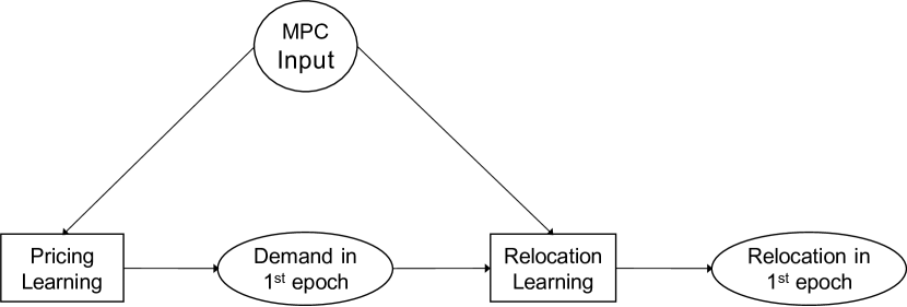
Figure 4: The Learning Methodology.

4.2 Learning Relocation Decisions

The relocation decisions are obtained in four steps: aggregation, learning, feasibility restoration, and disaggregation.

Aggregation

The relocation decision vector $[x^{r}_{ij1}]_{i,j\in Z}$ is often sparse, with most relocations occurring between a few low-demand and high-demand zones. To reduce sparsity, $x^{r}_{ij1}$ is first aggregated to the zone level. More precisely, two metrics are learned for each zone $i$: (1) the number of vehicles relocating from $i$ to other zones, i.e., $y^{o}_{i}:=\sum_{j\in Z,j\neq i}x^{r}_{ij1}$, and (2) the number of vehicles relocating to $i$ from other zones, i.e., $y^{d}_{i}:=\sum_{j\in Z,j\neq i}x^{r}_{ji1}$. These two metrics can be both non-zero at the same time: an idle vehicle might be relocated from $i$ to another zone for serving a request in the near future, and another vehicle could come to $i$ to serve a later request. This aggregation reduces the output dimension from $|Z|^{2}$ to $2|Z|$.

Learning

The relocation-learning algorithm takes the MPC inputs and the predicted first-epoch demand from the pricing learning algorithm. It predicts the aggregated relocation decisions $\mathbf{y}=[y^{d}_{i},y^{o}_{i}]_{i\in Z}$. In general, these predicted decisions are not feasible and violate the flow balance constraints.

Feasibility Restoration

The feasibility restoration turns the predictions $\mathbf{\hat{y}}=[\hat{y}^{o}_{i},\hat{y}^{d}_{i}]_{i\in Z}$ into feasible relocation decisions that are integral and obey the (hard) flow balance constraints. This is performed in three steps. First, $\hat{y}^{o}_{i}$ and $\hat{y}^{d}_{i}$ are rounded to their nearest non-negative integers. Second, to make sure that there are not more relocations than idle vehicles, the restoration sets $\hat{y}^{o}_{i}=\min\{\hat{y}^{o}_{i},V_{i1}\}$. Third, $\hat{y}^{o}_{i}$ and $\hat{y}^{d}_{i}$ must satisfy the flow balance constraint, e.g., $\sum_{i\in Z}\hat{y}^{o}_{i}=\sum_{i\in Z}\hat{y}^{d}_{i}$: this is achieved by setting the two terms to be the minimum of the two, by randomly decreasing some non-zero elements of the larger term.

Disaggregation Through Optimization

The previous steps produce a feasible relocation plan $[\hat{y}^{d}_{i},\hat{y}^{o}_{i}]_{i\in Z}$ at the zone level. The disaggregation step reconstructs the zone-to-zone relocation via a transportation optimization. The model formulation is given in Figure 5. Variable $z_{ij}$ denotes the number of vehicles to relocate from $i$ to $j$, and constant $c_{ij}$ represents the corresponding relocation cost. The model minimizes the total relocation cost to consolidate the relocation plan. The solution $z_{ij}$ is implemented by the ride-hailing platform in the same way as $x^{r}_{ij1}$ from the MPC. Note that $z_{ii}$ should be 0 for all $i$ since $\hat{y}^{d}_{i}$ and $\hat{y}^{o}_{i}$ denote relocations into and out of each zone. However, the problem in that form may be infeasible. By allowing the $z_{ii}$’s to be positive and assigning a large value to the relocation costs $c_{ii}$, the problem is always feasible, total unimodular, and polynomial-time solvable (Rebman 1974). As a result, the NP-hard MPC optimization is replaced by a learning methodology that produces an approximate solution in polynomial time.

$$\min\quad \sum_{i,j\in Z}c_{ij}z_{ij}$$

s.t. $$\sum_{j\in Z}z_{ij}=\hat{y}^{o}_{i},\quad \forall i\in Z$$

$$\sum_{j\in Z}z_{ji}=\hat{y}^{d}_{i},\quad \forall i\in Z$$

$$z_{ij}\in\mathbb{Z^{+}},\quad \forall i,j\in Z$$

Figure 5: The Transportation Problem for Disaggregation.

5 Experimental Results

The learning framework is evaluated on Yellow Taxi Data in Manhattan, New York City (NYC 2019). The learning models are trained from $2017/01$ to $2017/05$ and tested in $2017/06$. Section 5.1 reviews the simulation environment, Section 5.2 presents the learning results, and Section 5.3 evaluates the performance of the learned policy.

5.1 Simulation Environment

The end-to-end ride-hailing simulator reviewed in Section 3 is the basis of the experimental evaluation. The Manhattan area is partitioned into a grid of cells of $200$ squared meter and each cell represents a pickup/dropoff location. Travel times between the cells are queried from OpenStreetMap (2017). The fleet is fixed to be $1600$ vehicles with capacity $4$, distributed randomly among the cells at the beginning of the simulation. Riders must be picked up in 10 minutes and matched to a vehicle in 5 minutes since their requests, after which they drop out. The routing algorithm batches requests into a time window and optimizes every 30 seconds. The MPC component is executed every $5$ minutes. It partitions the Manhattan area into $24$ zones and time into $5$-minute epochs. The time window contains $6$ epochs and riders can be served in $2$ epochs following their requests. The number of idle vehicles in each epoch is estimated by the simulator based on the current route of each vehicle and the travel times. The ride-share ratio is $W_{ij}=1.5$ for all $i,j\in Z$. Service weight and relocation penalty are $q^{p}(t,\rho)=0.5^{t}0.75^{\rho-t}$ and $q^{r}_{ij}(t)=0.001*0.5^{t}\eta_{ij}$ where $\eta_{ij}$ is travel time between zone $i$ and zone $j$ in seconds. Five demand multipliers $[1,0.75,0.5,0.25,0]$ are available for each zone and epoch.

The baseline demand $\mathbf{D}:=[D^{0}_{ijt}]_{i,j\in Z,t\in\mathcal{T}}$ for each origin-destination zone-pair and epoch is forecasted and used to derive demand corresponding to each demand multiplier $\{D^{k}_{ijt}\}_{k\in K}$. The design of demand forecasting is beyond the scope of this paper, but the next paragraphs briefly review the methodology. In the real world, the zone-to-zone demand within a short time horizon (e.g., 5-minute time interval) is highly sparse: most trips travel between a few hot spots. $\mathbf{D}$ is also high dimensional and has $|Z|^{2}$ entries. To tackle the challenges raised by high dimensionality and sparsity, the demand is first aggregated and predicted at the zone level. Once the zone-level demand is predicted, it is disaggregated to the zone-to-zone level based on historical trip destination distribution. For example, if $\mu_{ij}$ proportion of trips from zone $i$ goes to zone $j$, and $D_{it}$ is the demand prediction for zone $i$, the final zone-to-zone prediction $D^{0}_{ijt}$ is $D_{it}\times\mu_{ij}$ rounded to the nearest integer.

The zone-level demand is forecasted based on the zone demand observed in the last $k$ epochs and the zone demand observed in the last week for the same periods. For instance, when forecasting the demand between 7.55 am and 8.00 am on $2017/01/08$, the model uses the demand between 7.55 am and 8.00 am on $2017/01/01$. The forecasting model is an artificial neural network with mean squared error (MSE) loss and $l_{1}$ regularization, two fully-connected layers with $(256,256)$ hidden units and ReLU activation functions. It is trained on $2017/01-2017/05$ and tested on $2017/06$. The mean absolute error (MAE) and the symmetric mean absolute percentage error (SMAPE) for each zone on the test set are displayed in Figure 6. The mean squared error of the disaggregated zone-to-zone level prediction is 0.49.

The MPC’s pricing decisions are implemented at the level of demand multipliers: if MPC decides to keep $50\%$ demand in a zone, the simulation randomly selects $50\%$ requests in the current epoch and discards the rest. After the MPC decides zone-to-zone level relocations, a vehicle assignment optimization determines which individual vehicles to relocate by minimizing total traveling distances (see Riley, Van Hentenryck, and Yuan (2020) for details).

Of the routing, MPC, and vehicle assignment models, the routing model is the most computationally intensive since it operates at the individual (driver and rider) level as opposed to the zone level. Since all three models must be executed within 30 seconds, the platform allocates $20$ seconds to the routing optimization, $5$ seconds to the MPC, and $5$ seconds to the vehicle assignment. All the models are solved using Gurobi 9.0 with 6 cores of 2.1 GHz Intel Skylake Xeon CPU (Gurobi Optimization 2020).

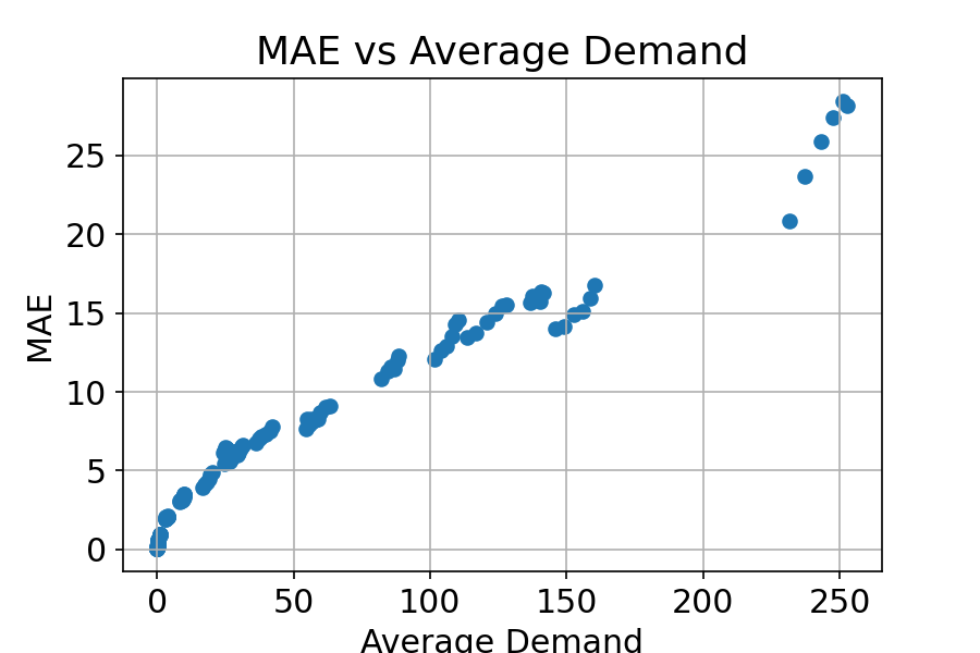
(a) MAE.

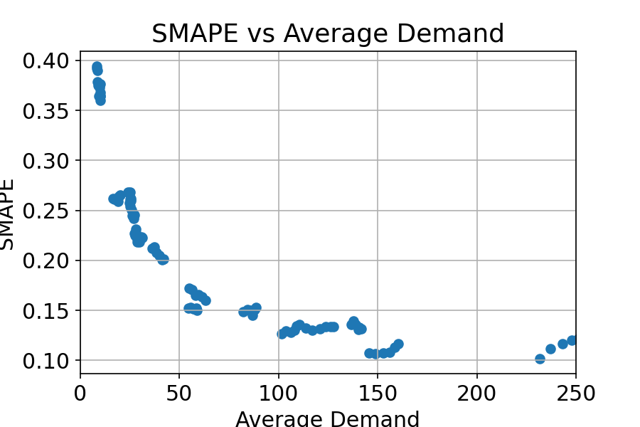
(b) SMAPE.

Figure 6: The Accuracy of the Demand Forecasting. Each Point Denotes the Average Demand and the MAE/SMAPE of a Zone on the Test Set.

Training Data

The learning policy is trained on Yellow Taxi data between $2017/01$ and $2017/05$. Each daily instance between 7 am and 9 am are selected as training instances. The total number of riders in these instances ranges from 10,000 to 50,000, representing a wide variety of demand scenarios in Manhattan. The instances are then perturbed by randomly adding/deleting certain percentage of requests to generate more training instances, where the percentages are sampled from a uniform distribution $U(-5,5)$. The instances are run by the simulator and the MPC results are extracted as training data.

5.2 Learning Results

In addition to the input features mentioned in Section 4.1, the pricing-learning algorithm also uses the following features: the difference between supply and demand in each zone in the first epoch under all demand multipliers, and the ratio between cumulative supply and cumulative baseline demand $[\tilde{V}_{it}/\tilde{D}^{0}_{it}]_{i\in Z,t\in\mathcal{T}}$ where $\tilde{V}_{it}=\sum_{\tau=1}^{t}V_{i\tau}$ and $\tilde{D}^{0}_{it}=\sum_{\tau=1}^{t}D^{0}_{i\tau}$. These additional features help improve the learning accuracy.

Four models were trained to learn the pricing and relocation decisions: random forest (RF), support vector regression (SVR), gradient boosting regression tree (GBRT), and deep neural network (DNN). The RF, SVR, and GBRT models were trained on 8000 data points and the DNN was trained on 35000 data points since fitting the DNN typically requires more data. All the models use the mean squared error (MSE) loss except SVR which uses epsilon-insensitive loss and $l_{2}$ regularization. The hyperparameters of each model were tuned through 5-fold cross-validation. The selected hyperparameters for the relocation models are: (kernel, regularization weight) = (radial basis function, 100), (max tree depth, number of trees) = (32, 200) for RF, (max tree depth, number of trees) = (64, 200) for GBRT, and two fully-connected hidden layers with (750, 1024) hidden units and hyperbolic tangent (tanh) activation functions for the DNN. The selected hyperparameters for the pricing models are: (kernel, regularization weight) = (radial basis function, 1000), (max tree depth, number of trees) = (64, 200) for RF, (max tree depth, number of trees) = (32, 100) for GBRT, and two fully-connected hidden layers with (750, 1024) hidden units and ReLU activation functions for DNN. The SVR, GBRT, and RF models were trained in scikit-learn package and the DNN model was trained in Pytorch by Adam optimizer with batch size $32$ and learning rate $10^{-3}$ (Pedregosa et al. 2011; Kingma and Ba 2014; Paszke et al. 2019).

Model	Relocation (MSE)	Pricing (MSE)	Pricing (0-1 Loss(%))
SVR	21.98	100.49	13.17
RF	21.69	101.29	13.32
GBRT	28.37	88.59	12.28
DNN	6.83	66.65	9.46

Table 2: Element-Wise Validation Errors.

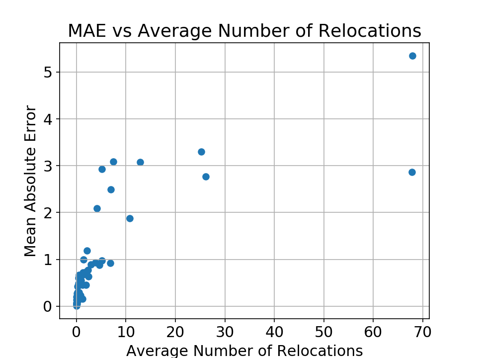
(a) Relocation Predictions.

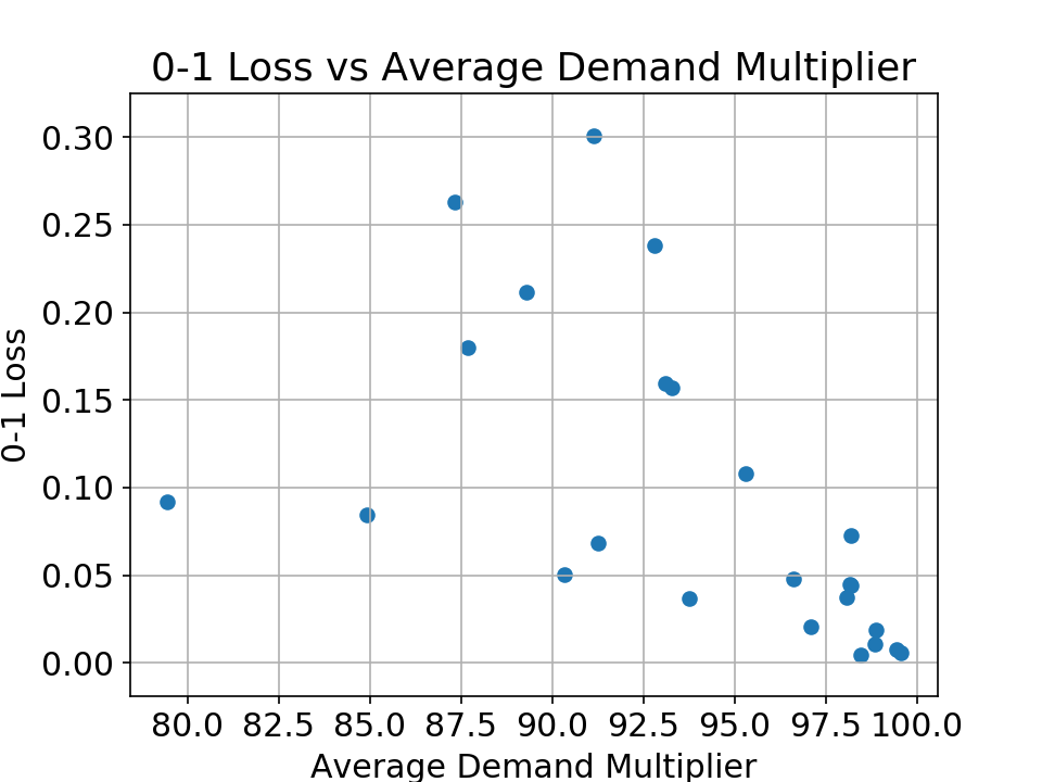
(b) Pricing Predictions.

Figure 7: MPC Decisions Predictions: Each Point on the Left Denotes the Average Relocations and the MAE of Relocation Predictions for a Zone. Each Point on the Right Denotes the Average Demand Multiplier and the 0-1 Loss of Pricing Predictions of a Zone.

The trained models were evaluated on a holdout validation set. The predictions are rounded to feasible solutions by the procedures described in 4.1 and 4.2. Element-wise errors after rounding are reported in Table 2, where the relocation models report the mean squared error loss (MSE) and the pricing models report both the MSE and the 0-1 loss (percentage of time that the rounded predictions were wrong). Since the DNN models achieved the highest accuracy in both cases, they were selected as the final model. The error for each zone under the DNN model is given in Figure 7. The prediction errors for all zones are reasonable, although a few zones exhibit higher loss than others. Overall these results indicate that the models successfully learned the MPC decisions.

5.3 The Benefits of Learning the MPC Model

(a) Drop Out Percentage.

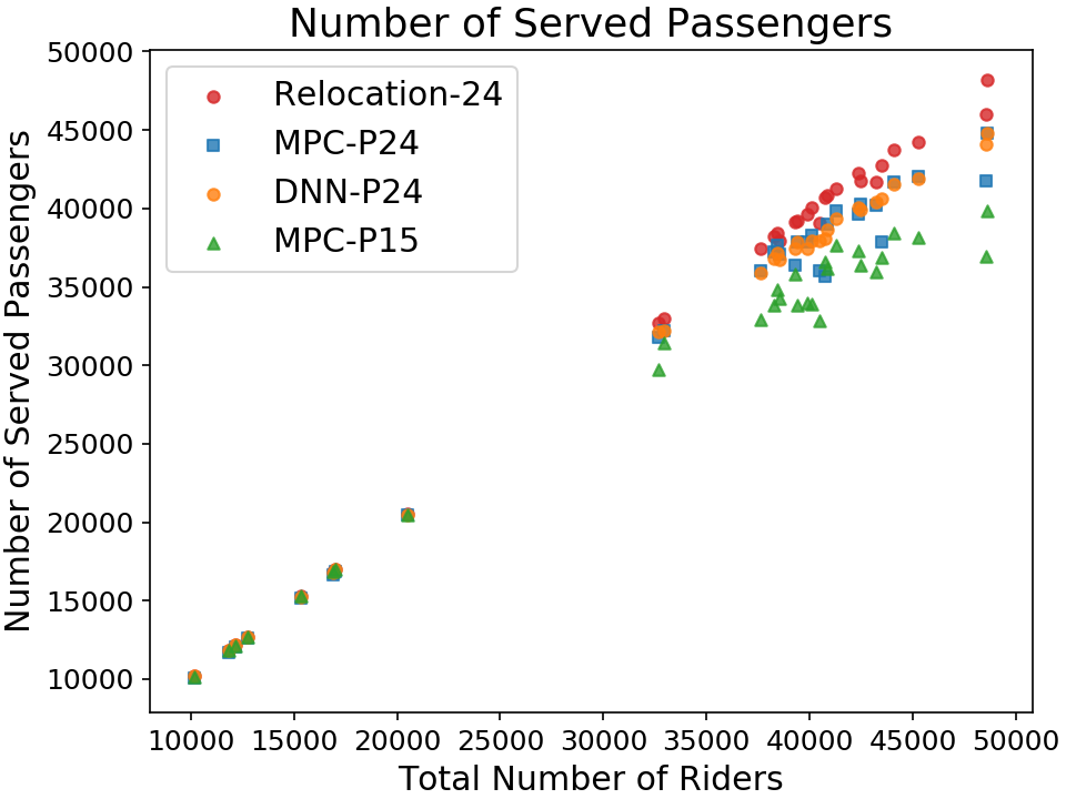
(b) Riders Served.

(c) Waiting Time Averages.

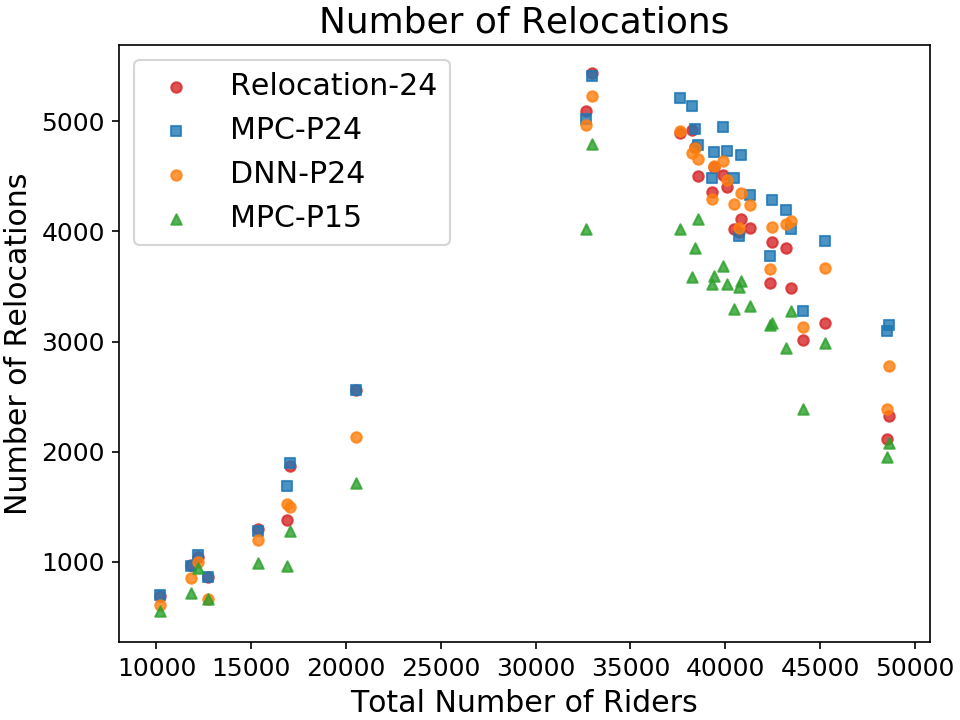
(d) Number of Relocations.

Figure 8: Evaluation Results of DNN-P24 and Its Comparison With Pure Optimization Approaches.

The benefits of learning the MPC optimization are evaluated on Yellow Taxi data in June, 2017. The proposed methodology (DNN-P24) is compared with the original MPC model with $24$ zones (MPC-P24), a lower-fidelity MPC model with $15$ clustered zones that represents what can be solved within the computational limit (MPC-P15), and a baseline that only performs relocation but not pricing (Relocation-24). All models but MPC-P24 are solved near optimally in $5$ seconds with 6 CPU cores as discussed in 5.1. MPC-P24, which cannot be solved near-optimally in $5$ seconds, is given more time and represents the ideal solution that cannot be achieved in real-time. In particular, 2.4% MPC-P24 instances failed to find a solution within 20% optimality gap in 5 seconds. The drop-out rate, number of riders served, rider waiting time averages, and the number of relocations are reported in Figure 8. In all instances, DNN-P24 achieves similar performance as MPC-P24. Both approaches ensure a drop-out rate near zero, whereas Relocation-24 loses increasingly more riders as the instance becomes larger. DNN-P24 and MPC-P24 also achieve lower average waiting times and serve similar number of riders as Relocation-24. In addition, they serve more riders than MPC-P15: on large instances with more than 25,000 riders, DNN-P24 serves on average $6.7\%$ more riders than MPC-P15 by pricing out fewer riders, demonstrating the benefits of higher model fidelity. DNN-P24 and MPC-P24 perform more relocations than MPC-P15 to serve more riders (finer spatial partition also unveils more opportunities for vehicle relocation). The solver times of the transportation optimization never exceed 0.093 seconds and the prediction time is also within fraction of a second. Overall, these promising results demonstrate that the proposed framework is capable of approximating high-fidelity MPC model efficiently, which leads to significant improvements in service quality.

6 Conclusion

Large-scale ride-hailing systems often combine real-time routing at the individual request level with a macroscopic Model Predictive Control (MPC) optimization for dynamic pricing and vehicle relocation. The MPC operates over a longer time horizon to anticipate the demand. The longer horizon increases computational complexity and forces the MPC to use coarser spatial-temporal granularity, which degrades the quality of its decisions. This paper addresses this computational challenge by learning the MPC optimization. The resulting machine-learning model serves as the optimization proxy, which makes it possible to use the MPC at higher spatial and/or temporal fidelity since the optimizations can be solved and learned offline. Experimental results on the New York Taxi data set show that the proposed approach serves 6.7% more riders than the original optimization approach due to its higher fidelity. A key factor behind the MPC model as well as the learning is the ability to predict future demand and supply accurately, which is challenging due to the fast-changing and volatile nature of real-time dynamics. Therefore, future works can focus on developing end-to-end learning and optimization systems that are robust to input uncertainty, possibly leveraging stochastic optimization and robust training techniques.

References

- Chen et al. (2019) Chen, H.; Jiao, Y.; Qin, Z.; Tang, X.; Li, H.; An, B.; Zhu, H.; and Ye, J. 2019. InBEDE: Integrating Contextual Bandit with TD Learning for Joint Pricing and Dispatch of Ride-Hailing Platforms. In 2019 IEEE International Conference on Data Mining (ICDM), 61–70. doi:10.1109/ICDM.2019.00016.
- Guériau and Dusparic (2018) Guériau, M.; and Dusparic, I. 2018. SAMoD: Shared Autonomous Mobility-on-Demand using Decentralized Reinforcement Learning. 2018 21st International Conference on Intelligent Transportation Systems (ITSC) 1558–1563.
- Gurobi Optimization (2020) Gurobi Optimization. 2020. Gurobi Optimizer Reference Manual. URL http://www.gurobi.com.
- Huang, de Almeida Correia, and An (2018) Huang, K.; de Almeida Correia, G. H.; and An, K. 2018. Solving the station-based one-way carsharing network planning problem with relocations and non-linear demand. Transportation Research Part C: Emerging Technologies 90: 1–17. ISSN 0968-090X. doi:https://doi.org/10.1016/j.trc.2018.02.020. URL https://www.sciencedirect.com/science/article/pii/S0968090X18302511.
- Iglesias et al. (2017) Iglesias, R.; Rossi, F.; Wang, K.; Hallac, D.; Leskovec, J.; and Pavone, M. 2017. Data-Driven Model Predictive Control of Autonomous Mobility-on-Demand Systems. CoRR abs/1709.07032. URL http://arxiv.org/abs/1709.07032.
- Jiao et al. (2021) Jiao, Y.; Tang, X.; Qin, Z.; Li, S.; Zhang, F.; Zhu, H.; and ping Ye, J. 2021. Real-world Ride-hailing Vehicle Repositioning using Deep Reinforcement Learning. ArXiv abs/2103.04555.
- Jin et al. (2019) Jin, J.; Zhou, M.; Zhang, W.; Li, M.; Guo, Z.; Qin, Z.; Jiao, Y.; Tang, X.; Wang, C.; Wang, J.; and et al. 2019. CoRide: Joint Order Dispatching and Fleet Management for Multi-Scale Ride-Hailing Platforms. Proceedings of the 28th ACM International Conference on Information and Knowledge Management doi:10.1145/3357384.3357978. URL http://dx.doi.org/10.1145/3357384.3357978.
- Kingma and Ba (2014) Kingma, D.; and Ba, J. 2014. Adam: A Method for Stochastic Optimization. International Conference on Learning Representations .
- Lei, Jiang, and Ouyang (2019) Lei, C.; Jiang, Z.; and Ouyang, Y. 2019. Path-based dynamic pricing for vehicle allocation in ridesharing systems with fully compliant drivers. Transportation research procedia 38: 77–97.
- Lei, Qian, and Ukkusuri (2020) Lei, Z.; Qian, X.; and Ukkusuri, S. V. 2020. Efficient proactive vehicle relocation for on-demand mobility service with recurrent neural networks. Transportation Research Part C: Emerging Technologies 117: 102678. ISSN 0968-090X. doi:https://doi.org/10.1016/j.trc.2020.102678. URL https://www.sciencedirect.com/science/article/pii/S0968090X20305933.
- Liang et al. (2021) Liang, E.; Wen, K.; Lam, W.; Sumalee, A.; and Zhong, R. 2021. An Integrated Reinforcement Learning and Centralized Programming Approach for Online Taxi Dispatching. IEEE Transactions on Neural Networks and Learning Systems doi:10.1109/TNNLS.2021.3060187.
- Lin et al. (2018) Lin, K.; Zhao, R.; Xu, Z.; and Zhou, J. 2018. Efficient Large-Scale Fleet Management via Multi-Agent Deep Reinforcement Learning. In Proceedings of the 24th ACM SIGKDD International Conference on Knowledge Discovery and Data Mining, KDD ’18, 1774–1783. New York, NY, USA: Association for Computing Machinery. ISBN 9781450355520. doi:10.1145/3219819.3219993. URL https://doi.org/10.1145/3219819.3219993.
- Ma, Fang, and Parkes (2019) Ma, H.; Fang, F.; and Parkes, D. C. 2019. Spatio-Temporal Pricing for Ridesharing Platforms. In Proceedings of the 2019 ACM Conference on Economics and Computation, EC ’19, 583. New York, NY, USA: Association for Computing Machinery. ISBN 9781450367929. doi:10.1145/3328526.3329556. URL https://doi.org/10.1145/3328526.3329556.
- Miao et al. (2015) Miao, F.; Lin, S.; Munir, S.; Stankovic, J.; Huang, H.; Zhang, D.; He, T.; and Pappas, G. 2015. Taxi Dispatch with Real-Time Sensing Data in Metropolitan Areas — a Receding Horizon Control Approach. IEEE Transactions on Automation Science and Engineering 13. doi:10.1145/2735960.2735961.
- NYC (2019) NYC. 2019. NYC Taxi & Limousine Commission - Trip Record Data. URL http://www.nyc.gov/html/tlc/html/about/trip“˙record“˙data.shtml. Accessed: 2020-10-01.
- Oda and Joe-Wong (2018) Oda, T.; and Joe-Wong, C. 2018. MOVI: A Model-Free Approach to Dynamic Fleet Management. IEEE INFOCOM 2018 - IEEE Conference on Computer Communications 2708–2716.
- OpenStreetMap (2017) OpenStreetMap. 2017. Planet dump retrieved from https://planet.osm.org. URL https://www.openstreetmap.org. Accessed: 2020-10-01.
- Paszke et al. (2019) Paszke, A.; Gross, S.; Massa, F.; Lerer, A.; Bradbury, J.; Chanan, G.; Killeen, T.; Lin, Z.; Gimelshein, N.; Antiga, L.; Desmaison, A.; Kopf, A.; Yang, E.; DeVito, Z.; Raison, M.; Tejani, A.; Chilamkurthy, S.; Steiner, B.; Fang, L.; Bai, J.; and Chintala, S. 2019. PyTorch: An Imperative Style, High-Performance Deep Learning Library. In Wallach, H.; Larochelle, H.; Beygelzimer, A.; d'Alché-Buc, F.; Fox, E.; and Garnett, R., eds., Advances in Neural Information Processing Systems 32, 8024–8035. Curran Associates, Inc. URL http://papers.neurips.cc/paper/9015-pytorch-an-imperative-style-high-performance-deep-learning-library.pdf.
- Pedregosa et al. (2011) Pedregosa, F.; Varoquaux, G.; Gramfort, A.; Michel, V.; Thirion, B.; Grisel, O.; Blondel, M.; Prettenhofer, P.; Weiss, R.; Dubourg, V.; Vanderplas, J.; Passos, A.; Cournapeau, D.; Brucher, M.; Perrot, M.; and Duchesnay, E. 2011. Scikit-learn: Machine Learning in Python. Journal of Machine Learning Research 12: 2825–2830.
- Qiu, Li, and Zhao (2018) Qiu, H.; Li, R.; and Zhao, J. 2018. Dynamic Pricing in Shared Mobility on Demand Service. arXiv: Optimization and Control .
- Rebman (1974) Rebman, K. R. 1974. Total unimodularity and the transportation problem: a generalization. Linear Algebra and its Applications 8(1): 11–24. ISSN 0024-3795. doi:https://doi.org/10.1016/0024-3795(74)90003-2. URL https://www.sciencedirect.com/science/article/pii/0024379574900032.
- Riley, Legrain, and Van Hentenryck (2019) Riley, C.; Legrain, A.; and Van Hentenryck, P. 2019. Column Generation for Real-Time Ride-Sharing Operations. In Rousseau, L.-M.; and Stergiou, K., eds., Integration of Constraint Programming, Artificial Intelligence, and Operations Research, 472–487. Springer International Publishing.
- Riley, Van Hentenryck, and Yuan (2020) Riley, C.; Van Hentenryck, P.; and Yuan, E. 2020. Real-Time Dispatching of Large-Scale Ride-Sharing Systems: Integrating Optimization, Machine Learning, and Model Predictive Control. In Proceedings of the Twenty-Ninth International Joint Conference on Artificial Intelligence, IJCAI-20, 4417–4423. International Joint Conferences on Artificial Intelligence Organization. doi:10.24963/ijcai.2020/609. URL https://doi.org/10.24963/ijcai.2020/609.
- Verma et al. (2017) Verma, T.; Varakantham, P.; Kraus, S.; and Lau, H. C. 2017. Augmenting Decisions of Taxi Drivers through Reinforcement Learning for Improving Revenues. In ICAPS.
- Zhang, Rossi, and Pavone (2016) Zhang, R.; Rossi, F.; and Pavone, M. 2016. Model predictive control of autonomous mobility-on-demand systems. In 2016 IEEE International Conference on Robotics and Automation (ICRA), 1382–1389. doi:10.1109/ICRA.2016.7487272.