Kanzelhöhe Observatory: instruments, data processing and data products

1 Introduction

Kanzelhöhe Observatory for Solar and Environmental Research (KSO) of the University of Graz is located on a mountain ridge at an altitude of 1526 m a.s.l. near Villach in southern Austria. The observatory was founded in 1943 as part of a network of solar observatories operated by the German Airforce (Pötzi et al., 2016; Jungmeier, 2017). The discovery of Mögel and Dellinger (Dellinger, 1935) that solar flares can cause ionospheric disturbances by a sudden increase of the ionisation of the D-layer in the ionosphere, such that blackouts of radio communications can occur, made it necessary to investigate such phenomena to arrive at a better understanding and predictions of these effects (Seiler, 2007).

Solar observations at KSO date back to 1943. In the early years of the observatory, most observations were performed using a heliostat guiding the light beam down to a laboratory in the basement, where a projection device for sunspot drawings and a spectroheliograph (Siedentopf, 1940; Comper, 1958) were installed. In a second tower a coronagraph was operated (Comper and Kern, 1957), which was transferred in 1948 to the top of the Gerlitzen mountain (1 900 m a.s.l). First observations in the H$\alpha$ spectral line were made visually at the spectroheliograph. In 1958, a Zeiss-Lyot monochromator acquired on occasion of the International Geophysical Year made photographic observations in the H$\alpha$ line possible. In addition, a piggy-back mounted telescope on the coronagraph was used to record the photosphere on glass plates. A more detailed description about the early observations at KSO can be found in Kuiper (1946). Corona observations were suspended in 1964 as the seeing conditions on top of the mountain worsened. In 1973 all observations were transferred to the northern tower (Figure fig:obs) offering better seeing conditions (Pötzi et al., 2016).

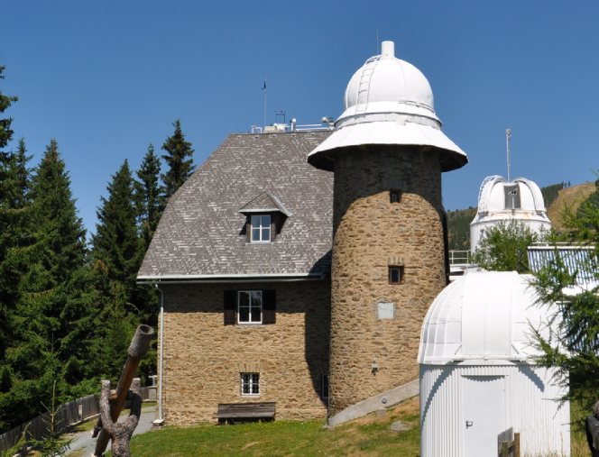
Figure 1.: Kanzelhöhe Observatory today: The heliostat was installed in the southern tower (leftmost) in the northern tower (open dome in background)

a small telescope for testing purposes replaced the coronagraph after 1948. Since 1973 all observations are performed in the northern tower. fig:obs

In pre-digital times, i.e. up to the year 2000, observing was a combination of “manual” and “visual” work. Photographs were made on glass plates (later on sheet film and 36 mm film), which had to be manually exposed and afterwards developed. Observations at the coronagraph were on the one hand noted on special form sheets describing the intensity in the green (5303 Å) and red (6874 Å) corona lines (cf. Waldmeier1942) and on the other hand also photographs of the corona intensity in H$\alpha$ (FWHM=20 Å) were taken (Comper and Kern, 1957). White-light observations on photographic material date back to 1943, images were recorded irregularly, mostly on occasion of big sunspots. From 1989 on every day at least three images were taken using the photoheliograph in the northern tower (Pettauer, 1990). Patrol observations of H$\alpha$ images started in 1958 on an irregular basis and were already automatized in 1973 at a cadence of one image every 4 minutes on 35 mm film rolls. Large parts of the data have been digitized like the white-light images on sheet film from 1989 to 2007 (Pötzi, 2010) and the H$\alpha$ film rolls from 1973 to 2000 (Pötzi, 2007). Digitising the corona images and the H$\alpha$ images before 1973 is not planned as the effort is too high and the quality of the data is often very low. Digitizing the white-light images on glass plates between 1943 and 1970 is planned in the future. Sunspot drawings have always been made by hand and they will not be subject to automatized procedures in order to contain long-term consistency, as is explained in detail by Clette et al. (2014). Nonetheless all drawings are scanned immediately and published in our archive. In 2010 full disc observations in the Ca ii K line widened out the monitoring of the solar activity.

KSO data are used for a variety of scientific research topics, due to the data reaching back over several cycles, their continuous and high data quality as well as for being freely available to the community via the KSO data archive (https://cesar.kso.ac.at). The main research topics for which KSO data are studied are the following. H$\alpha$ data are in particular used for the study of energetic events such as solar flares (e.g., Wang et al., 2003; Veronig et al., 2006b; Vršnak et al., 2006b; Miklenic et al., 2007; Pötzi et al., 2015; Thalmann et al., 2015; Joshi et al., 2017; Temmer et al., 2017; Hinterreiter et al., 2018; Tschernitz et al., 2018), filament eruptions and dynamics (e.g. Maričić et al., 2004; Möstl et al., 2009; Zuccarello et al., 2012; Su et al., 2012; Filippov, 2013; Yardley et al., 2016; Aggarwal et al., 2018), Moreton waves (e.g., Pohjolainen et al., 2001; Warmuth et al., 2001; Vršnak et al., 2006a; Veronig et al., 2006a) as well as for long-term evolution of the distributions of prominences and polar crown filaments (e.g., Rybák et al., 2011; Xu et al., 2018, 2021; Chatterjee et al., 2020). Sunspot drawings are used for the derivation of (hemispheric) sunspot numbers and solar cycle studies (e.g., Temmer, Veronig, and Hanslmeier, 2002; Temmer et al., 2006; Clette et al., 2014; Clette and Lefèvre, 2016; Pötzi et al., 2016; Chatzistergos et al., 2017; Chowdhury et al., 2019; Veronig et al., 2021). White light images and sunspot drawings are used for deriving solar differential rotation rates and meridional flows (e.g.  Hanslmeier and Lustig, 1986; Lustig and Hanslmeier, 1987; Poljančić Beljan et al., 2017; Ruždjak et al., 2018) as well as for sunspot catalogs (Baranyi, Győri, and Ludmány, 2016). Ca ii K images are used for long-term solar irradiance investigations (e.g., Chatzistergos et al., 2020) and flare studies (e.g., Veronig and Polanec, 2015; Sindhuja et al., 2019).

2 Instruments and Data acquisition

2.1 Instruments

The main instrument at KSO is the patrol instrument, which is in operation since 1973 in the northern tower. This instrument carries four telescopes (Figure fig:UEWI) on a parallactic mounting:

• Ca ii K:
  A refractor with a diameter of 100 mm and a focal length of 1 500 mm. The system is protected by a dielectric energy reflection filter. The main filter was originally a DayStar etalon, which degraded in 2012 and was replaced by a Lunt B1800 Ca-K module in 2013. As the specifications required a F/20 configuration in order to guarantee the designed bandwidth (Hirtenfellner-Polanec et al., 2011) the aperture front lens was reduced to 70 mm.

• White-light:
  A refractor with an objective lens of 130 mm and a focal length of 2000 mm. The broadband filter with a FWHM of 100 Å is centred in the green range of the visual electromagnetic spectrum at 5 460 Å Otruba, Freislich, and Hanslmeier (2008). The telescope is based on the Kanzelhöhe Photoheliograph (PhoKa) which went into operation in 1989 and was described in detail in Pettauer (1990). In order to compensate for thermal expansion the camera position is adapted each day.

• H$\alpha$:
  A refractor with 100 mm diameter and a focal length of 1 950 mm. The objective lens is coated with gold serving as heat filter and the Zeiss Lyot H$\alpha$ filter with a central wavelength of 6 562.8 Å and a FWHM of 0.7 Å is placed behind a broadband H$\alpha$ pre-filter (Otruba and Pötzi, 2003; Pötzi et al., 2015). A beam-splitter provides the possibility to attach a second camera, which can be used for, e.g., ultra-high cadence observations with several images per second additional to the standard patrol observations.

• Drawing Device:
  The drawing device is mounted near the declination axis of the telescope, which makes it comfortable to produce the drawing on the projected image (which has a diameter of 25 cm) and also minimizes the forces applied to the telescope by the drawing procedure itself. The drawing is used for obtaining the relative sunspot number, which is sent to SILSO (Sunspot Index and Long-term Solar Observations) World Data Center at the Royal Observatory of Belgium for calculating the International Sunspot Number (ISN), more details can be found in Pötzi et al. (2016).

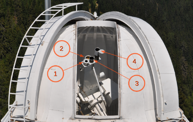
Figure 2.: The KSO solar patrol instrument in the northern tower carries four telescopes: (1) - Ca ii K, (2) - White-light, (3) - H$\alpha$, (4) - Drawing device. The slit of the dome moves automatically with the telescope.fig:UEWI

An overview of the telescope configurations is given in Table tbl:patrol. In the current configuration the same CCD camera type (2048$\times$2048 pixels with 4 096 intensity levels) is used for data acquisition (further technical details on the camera specification can be found in Appendix camera). Identical grabbing software and almost the same processing software is implemented for all observation types. This configuration reduces the workload in handling, maintaining and keeping up to date. As a measure of precaution we have acquired additional CCD cameras of the same type for immediate replacement if necessary.

Table 1.: The current and former configurations of the telescopes on the KSO solar patrol instrument:tbl:patrol

c   urrent configurations (2021)
	H$\alpha$	White-light	Ca ii K
aperture	100 mm	130 mm	70mm
focal length	2000 mm	1 950 mm	1 500 mm
central wavelength	6 562.8 Å	5 450 Å	3 933.7Å
FWHM	0.7 Å	100 Å	20 Å
CCD camera	all telescopes: JAI Pulnix RM-4200GE
image size	2 048 $\times$ 2 048 pixel
bit depth	12bit
observing cadence	10 images/min	3 images/min	10 images/min
exposure time	1.5 - 25 ms	2.2 - 25 ms	1.5 - 35 ms
operating since	June 2008	August 2015	July 2010
former configurations
CCD camera	Pulnix TM-1010	JAI Pulnix TM-4100CL
image size	1 000 $\times$ 1 1012 pixel	2 048 $\times$ 2 048 pixel
bit depth	10bit	10bit
observing cadence	10 images/min	1 image/min
exposure time	2.5 - 33 ms	3.5 - 25 ms
operating since	July 2005	July 2007
CCD camera	Pulnix TM-1001
image size	1 008 $\times$ 1 016 pixel
bit depth	8bit
observing cadence	1 image every 100 sec
exposure time	3.5 - 66 ms
operating since	December 1998

2.2 Data acquisition

The data acquisition software is written in C++ and makes use of commercial camera control libraries (Common Vision Blox from Stemmer Imaging). The user interface (Figure fig:interf) is kept as simple as possible but also offers many additional features, which are not used in standard patrol mode. The observer marks a rectangular box on the solar disc: during enhanced solar activity this box is placed over an active region and in case of quiet solar conditions the box is placed at solar disc centre. This AOI (area of interest) is used for calculating the exposure time and the image contrast. The mean brightness in this AOI is set to a fixed value (600 counts for H$\alpha$ in order to avoid saturation of the CCD chip in case of bright flares, 2 000 for white-light and 1 000 for Ca ii K). Based on these pre-defined mean values, the exposure time for the camera is calculated. As the camera is much faster (6 to 7 images per second) than the typical image cadence (6 seconds) the system can use frame selection and profits from very short moments of better seeing conditions (Scharmer, 1989). For this purpose the image contrast in the AOI is calculated, i.e., the camera selects from a sequence of about 10 images the one that has the highest rms contrast.

Before and after the daily observations, when the objective lens is protected with the dust cover, a dark current image is made. For this purpose the exposure time is fixed to 3 msec, which corresponds to an average exposure time in patrol mode. Dark current images during the observation time are not possible as there always falls light onto the CCD chip, since the cameras are not equipped with a mechanical shutter. The button “SnapFixExpTimes” starts a series of images at 5 msec, 20 msec and 50 msec exposure time. It is used especially for the H$\alpha$ camera in order to get an image of the lower corona in H$\alpha$ light by overexposing the solar disc. These images are used as backup and additional data for the solar prominence catalogue of the Lomnický Štít Observatory (Rybák et al., 2011). All images are stored directly in a live archive on a raid system as raw FITS files and JPEG files for a quick inspection.

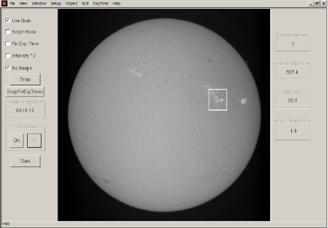
Figure 3.: The data acquisition interface for the H$\alpha$ camera (26 May 2021), it is the same for the other cameras. In standard patrol observation mode the user has just to click the “On” button and the observation program runs automatically. The white box indicates the selected AOI.fig:interf

3 Data processing

3.1 Data pipeline

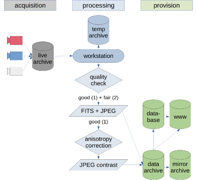
Figure 4.: Flow diagram of the data pipeline for solar images at KSO. Each of the three branches – acquisition, processing and provision – is running on a separate system. All systems work in parallel, the whole process takes not more than 5 seconds for an individual image from acquisition to provision. fig:pipel

Figure fig:pipel shows the data pipeline for images from their recording at the CCD camera to the main archive. The whole process can be divided into three steps: data acquisition, data processing and data provision. Each step is performed by a separate workstation, which work in parallel. The whole process from data acquisition to the provision of the processed data takes about 5 seconds per image. H$\alpha$ images undergo a second step of processing (FITS files of quality 1) in order to automatically detect and characterize flares and filaments in the real-time observations. This procedure is elaborated in detail in Pötzi et al. (2015) and evaluated in Pötzi, Veronig, and Temmer (2018).

In the following, we describe the standard processing pipeline, which every image grabbed by one of the CCD cameras passes through. In order to keep the system simple and to reduce maintenance and work load for updates all following steps are performed by almost the same script that is executed three times in parallel, one instance for each of the 3 CCD cameras. This script calls individual programs, which process the images or manage the database. The scripts are started before sunrise and just wait for new images appearing in the live archive for processing until they stop after sunset.

Step 1: Before processing, the observed image is transferred from the live archive to the temporary archive, which can hold up to nearly one year of the raw observation data. In order to free space for new images, successively the oldest ones in this temporary archive are deleted. Normally in the live archive there is only the latest image. If there is some interruption or delay in the processing pipeline, a larger amount of images can accumulate there. But also in this case only the latest image is processed and transferred in order to prevent any delay in data provision. All images that remain on the live archive until the end of the observation day are processed later. The temporary archive is used as an emergency backup, in case the processing fails due to some unexpected reason or if even images of low quality can be of interest for inspection of some extraordinary solar events. It can also be of interest in developing algorithms for the parametrization of image quality or classification purposes (Jarolim et al., 2020), see Section subimqual.

Step 2: A crucial step is the quality check (described in detail in Section subimqual), that selects the images that are processed and stored in the main data archive. This procedure should be fast and deliver stable results independently of the solar cycle phase or time of day. The images are categorized as good (quality=1), fair (2) and bad. Images of quality 1 are suitable for all further automatic processing steps, whereas quality 2 images can still be used for visual inspection.

Step 3: Images of quality 2 (fair image quality, suitable for visual inspections) and of quality 1 (good quality) get a an updated FITS header containing all relevant image information, see Appendix FITS) and a normal contrast JPEG image is produced for real time display. The JPEG image is centred, contrast enhanced by unsharp masking and contains logos, date and time stamp and is overlaid with a heliographic grid. The FITS file and the JPEG file are stored in the data archive.

Step 4: From images of quality 1 additionally high contrast JPEG images are generated, i.e. they are corrected for global anisotropies in order to provide a homogeneous contrast across the solar disc (details in Section inhomoCorr). Like normal contrast images, they are overlaid with a heliographic grid, they contain logos and a date and time stamp. These images are also stored in the data archive.

Dark current is not subtracted from the images, This effect cannot be seen in the JPEG images as the dark current correponds to a very low level of additional noise, which is removed by the JPEG compression algorithm. Flat field is also not applied for reasons explained in Section subFF.

3.2 Image quality detection

subimqual

In this section we describe the details of the image quality determination, which is in operation at KSO. The quality estimate makes use of a variety of properties of the images, which allow us to characterize the quality on both global and local scales:

• exposure time

• mean intensity in AOI

• solar limb and radius determination, see detlimb

• large-scale image inhomogeneities, see iminho

• image sharpness, see detsharp

Since the exposure time is automatically controlled and set in a way that the AOI has a pre-defined mean count value, it is sensitive to clouds and to a low elevation of the Sun above the horizon. The mean intensity in the AOI can vary when clouds move very fast across the solar disc, in such cases the exposure time adjustment can be too slow, and the image can be under- or overexposed.

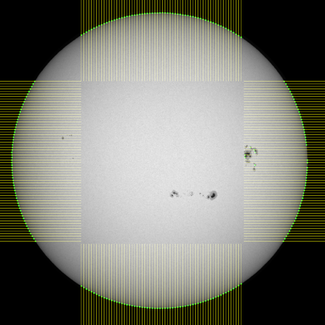
Figure 5.: Illustration of the determination of the solar limb and centre. The maximum gradient (green dots) of the intensity in 64 profiles for each direction is calculated. A circle fit through these points gives the radius and the centre coordinates of the solar disc. In this white-light image from 6 September 2017 large sunspots lead to some outliers in the first step of the limb detection, which are automatically removed in the following iterative steps.fig:limbp

3.2.1 Detection of solar limb and radius

detlimb

This procedure is an enhanced version of the method published by Veronig et al. (2000) and is based on the limb detection by finding the limb points as the maximum gradient of intensity profiles in $x$ and $y$ direction. To get stable results the profiles are smoothed over 7 pixels before the gradient is applied via a morphological operation. For reducing the calculation time only 64 profiles from each direction are generated (see Figure fig:limbp). Through these limb points a circle is fitted using Taubins method (Taubin, 1991). This method is very stable and fast and it needs only a limited number of points for the fit. The circle fit tries to minimize

$$\Omega=\sum_{i=1}^{n}d_{i}^{2}$$ (1)

where

$$d_{i}=\sqrt{(x_{i}-a)^{2}+(y_{i}-b)^{2}}-R_{\odot}$$ (2)

which is the geometric distance from each detected limb point ($x_{i}$,$y_{i}$) on the solar limb to the fitting circle whose centre and radius are ($a$,$b$) and $R_{\odot}$, respectively. As a measure for the quality of the circle fit we obtain the value $\sigma$ which is the rms of $d_{i}$. In order to improve the circle fit and to obtain a robust solution, outliers are iteratively removed. I.e., in the first iteration limb points with a distance from the fitted circle $d\geq R_{\odot}/30$ are excluded and a new circle fit is performed. If $\sigma$ is still $\geq 2$ this procedure is repeated with $d\geq R_{\odot}/100$ and if necessary also with $d\geq R_{\odot}/200$.

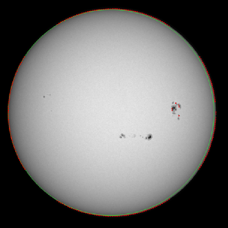
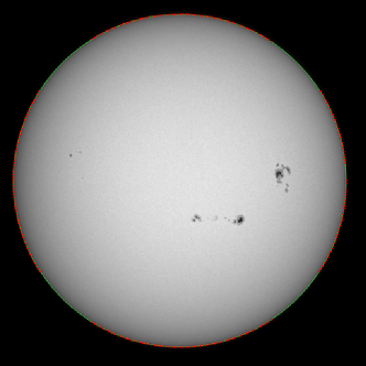
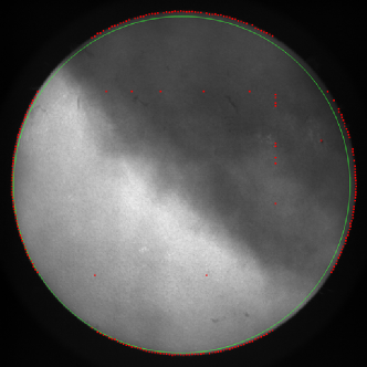
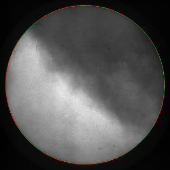
Figure 6.: Illustration of the determination of the solar limb and centre. Detected limb points (red dots) and limb fit (green circle) obtained after the first (left panels) and final (right panels) iterations. In the first row a white-light image from 6 September 2017 at good observation conditions shows already after one iteration a good fit for the solar limb. In the second row clouds disturbed the H$\alpha$ observations on 31 December 2020 and therefore three iterations where necessary to obtain a good circle fit.fig:limb

In Figure fig:limb two examples demonstrate the workflow of this process. The white-light image at good observing conditions in the first row needs just one iteration for finding sufficiently precise solar disc parameters, the outliers near the large sunspot group (red dots) are removed immediately. In the second row an H$\alpha$ image is strongly disturbed by clouds. In this case all three iteration steps are needed in order to obtain a good circle fit through the limb. As the profiles used for detection of the limb points go from the image border one fourth into the image (cf. Figure fig:limbp), some of the detected points are aligned in almost a straight line (red dots in left image of the second row in Figure fig:limb). These “outliers” are responsible for the bad circle fitting (overplotted green circle). Therefore in the next iterations outliers are removed and the circle fit is recalculated. The right image shows the result obtained in the last step, where the circle fit (indicated as green line) is within the required limits ($\sigma\leq 2$). We note that such image is not further processed. This is an example to demonstrate how robust this method is. We note that the result of this limb finding procedure is also used to fine-tuning the telescope guider. Thanks to this robustness, the telescope position can be maintained accurately to the centre of the solar disc also during cloudy periods.

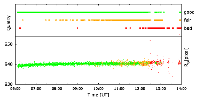
Figure 7.: H$\alpha$ image quality and solar radius determination for a full observation day (11 April 2020). Top panel: The observed H$\alpha$ filtergrams are colour coded by the determined image quality. Bottom panel: The radius determinations are coloured according to the corresponding image quality. This is a typical seeing situation during a fine sunny day at KSO, where the seeing conditions become worse during the day and cumulus clouds evolve in the afternoon. The data series plotted contains a total of 4204 images.fig:qualrad

Figure fig:qualrad shows the determined radius and the H$\alpha$ image quality for a complete observation day for the H$\alpha$ telescope (11 April 2020). In total 4 204 H$\alpha$ images were recorded on this day: 3 098 of quality class 1, 738 of class 2 and 375 of quality 3. One can see from the plot, that the observations get worse over the day. The observation conditions are commonly the best in the morning. In case of fine and sunny weather, over the day the rising air causes turbulences that decrease the seeing conditions. In the afternoon occurring cumulus clouds interrupt the observations, in most cases these clouds dissolve until the evening. The determined radius of the solar disc (bottom panel) reveals in general very stable results, with an average $R_{\odot}=940.16\pm 0.52$ pixels (determined from all images of quality class 1). The radius values in the morning and later in the afternoon are somewhat smaller due to refraction effects and less image motion. As one can also see, the radius distribution becomes wider when the image quality decreases.

3.2.2 Parametrization of large-scale image inhomogeneities

iminho

The detection of image inhomogeneities is normally a very computation expensive task, which can be done with structural bandpass filters (cf. Poetzi2015) or also with neural networks (Jarolim et al. (2020), see also Section GAN). For the real-time processing this method must be fast and effective. To accomplish this task, in the current implementation at KSO, the recorded and centred image is reduced to 2$\times$2 pixels and the ratio of the maximum to the minimum value of these pixels, the so called global quadrant intensity ratio ($fpr$), is computed. Images without any inhomogeneities should have a $fpr$ of nearly 1, active regions or filaments have only a small influence on this ratio as their area is in the range of maximum a few percent of the solar hemisphere. Clouds, however, can shift this ratio to values far larger than 1 as illustrated in Figure fig:fpr top right. A drawback of this method is that clouds uniformly distributed also lead to a value of about 1 (Figure fig:fpr top left). In such case other measures are needed to quantify the reduced image quality like the exposure time or the image sharpness.

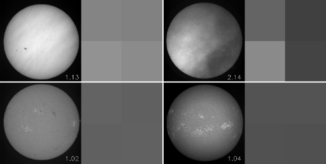
Figure 8.: Four examples for large-scale image inhomogeneity parametrization in white-light (upper left, 1 December 2020), H$\alpha$ (upper right – 31 December 2020, lower left – 29 January 2016) and Ca ii K (lower right – 7 January 2015) images. The full-disc images are reduced to 2$\times$2 pixels (right to each solar disc image) and the ratio of the maximum to the minimum of the 4 pixels is computed (annotated in each image). The images that are partially obstructed by clouds lead to high ratios, far higher than the optimum case of 1.fig:fpr

3.2.3 Parametrization of image sharpness

detsharp

Normally for the image sharpness the rms of the intensity distribution is used, but in case of the Sun this value changes considerably with the solar activity. The presence of filaments, active regions or flares produce substantially higher rms values compared to a quiet Sun. Therefore, for an alternative approach that works fully automatic, we use the central part of the solar disc, covering the central quarter of the image area, smooth it by convolving the subimage with a simple kernel consisting only of 1’s, e.g., a kernel of size 3 looks like:

$$k_{3}=\frac{1}{3^{2}}\left[\begin{array}[]{ccc}1&1&1\\ 1&1&1\\ 1&1&1\\ \end{array}\right]$$ (3)

For KSO images the kernel $k_{15}$ is used ($\approx$15 arcsec), which is the same as averaging pixels in a neighbourhood of 225 pixels. This smoothed subimage is then correlated with the original subimage. Sharpness values $S$ are then obtained by:

$$S=1\,000\times(1-r)$$ (4)

where $r$ is the Pearson’s correlation coefficient between the smoothed and the original subimage. The factor of 1 000 was introduced to obtain integer results in a typical range up to $\approx$100. The reasoning behind this method is the following: when the smoothing of the image does not substantially change the image, i.e. when the image was already unsharp before smoothing, the value of $r$ would be 1 and therefore $S=0$. Typical values are $S>50$ in case of quality class 1 H$\alpha$ images, whereas images in quality class 3 have $S<25$. These boundaries are lower in case of white-light and Ca ii K images.

3.2.4 Summary of quality determination

sumqual

The three quality levels are determined by single or combinations of the above parameters or procedures, e.g, for H$\alpha$ images:

• high exposure times ($exp\geq 18$ ms): quality class 3

• rms of solar radius determination $>5$ pixel: quality class 3

• global quadrant intensity ratio $>1.08$: quality class 3

• $exp$ $>5$ ms and rms of solar radius $>$ 3: quality class 3

• mean intensity in AOI $\leq 400$ or $\geq 1200$ counts: quality class 3

• image sharpness $<25$: quality class 3

• image sharpness $<50$: quality class 2

The settings for white-light and Ca ii K images differ slightly, like the mean intensity in the AOI has a much higher default value for white-light images as we do not expect large changes of image brightness, in contrast to H$\alpha$ images that may vary strongly during flares. The parameters defining the quality classes for each camera are listed in Appendix Section qualparam.

3.3 Quality parametrization with Generative Adversarial Networks

GAN

A different approach for image quality assessment of ground-based solar observations was presented by Jarolim et al. (2020), where the authors used a neural network to identify quality degradation. The method is based on generative-adversarial-networks (GANs) to model the true image distribution of high quality KSO H$\alpha$ observations and assessing deviations from it, such that atmospheric influences (e.g., clouds) result in large deviations. This metric is more objective in terms of the solar activity level. The method provides a human-like quality assessment that agrees in 98.5% of the cases with human assigned labels. The developed neural network provides a continuous image quality metric and a binary classification into high- and low-quality observations. In the upper panel of Figure fig:qualcomp we compare the image sharpness (defined in Section detsharp) with the continuous image quality value of the neural network. For comparison fixed thresholds in the image quality metric were set and additionally the binary classification to further distinguish between good (class 1) and fair (class 2) images was used (cf. Jarolim2020). The direct comparison shows that both assessment methods are in general in good agreement. The neural network shows a higher sensitivity for clouds, while it is less sensitive to the variations in seeing, in agreement with the objective for large scale image inhomogeneities. The fast performance of the neural network makes it suitable for the critical step of quality assessment in a real-time environment. The further extension to small scale quality estimations (e.g., seeing), multiple channels (e.g., white-light, Ca ii K) and the applicability to a real-time data pipeline are under investigation.

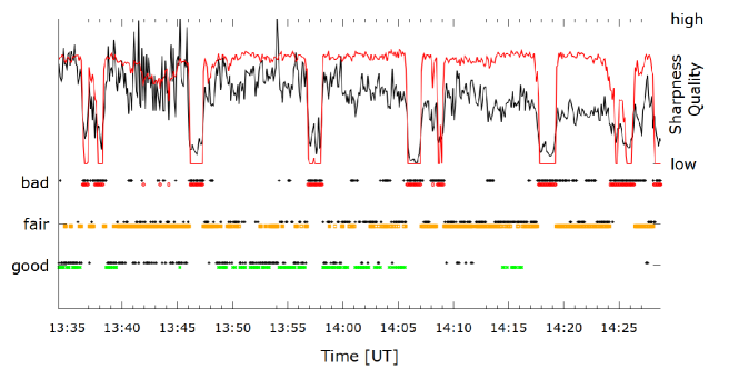
Figure 9.: Comparison of two different quality parametrization methods applied to KSO H$\alpha$  images on 26 January 2019. In the upper panel the quality value obtained with the GAN method (red) is compared to the sharpness value $S$ (black). The lower panel shows that the quality estimations dividing the images into three classes of both methods are in general in agreement. fig:qualcomp

3.4 Correction of large-scale image inhomogeneities

inhomoCorr

3.4.1 Centre-to-limb variation

In order to derive a centre-to-limb variation (CLV) profile we apply a median filter on each concentric ring of the solar disc with a width of one pixel. Features like sunspots, active regions or filaments do in general not have an effect on such a filter, as they are clearly smaller than the half length of such a concentric ring. However, close to the centre of the solar disc, these activity features can cover a substantial part of the rings. Thus, for robustness, for the inner rings a further post-processing should be applied, e.g., an interpolation via a CLV functional fitting as is described below. This procedure is computationally intensive, but as each ring can be handled independently the code can easily be parallelized.

According to Scheffler and Elsässer (1990) the CLV profile can theoretically be expressed as

$$I_{\beta}=\frac{1+\beta\cdot\cos\theta}{1+\beta}$$ (5)

where $I$ is the intensity, $\beta$ is the centre-to-limb variation factor and $\theta$ is the exit angle of the light (disc centre: $\beta=0$, limb: $\beta=\pi/2$). In order to use distances from the centre of the solar disc this equation can also be rewritten to

$$\ilabel{Eq:clv}I_{x}=\frac{1+b\cdot\cos(\arcsin(a\cdot x))}{1+b}$$ (6)

with $a$ as scale factor of the solar radius, $b$ as centre-to-limb variation factor and $x=r/R_{\odot}$. This formula does not describe the whole profile as the numerator is always larger than or equal one and the upper limit of the denominator is defined by $1+b$, which is in most cases smaller than 3.

By fitting the calulated CLV profile by Eq. Eq:clv, a complete smooth CLV profile can be obtained which is not affected by intensity fluctuations introduced by the individual rings. In order to avoid the potential effects of solar activity features (sunspots, flares, filaments) on the inner rings, we applied the fits to different subranges (avoiding the inner parts) and evaluated the robustness of the fit results, namely $[0-1]R_{\odot}$, $[0-0.97]R_{\odot}$, $[0.10-0.97]R_{\odot}$, $\ldots[0.70-0.97]R_{\odot}$. These evaluations were done with KSO white light and H$\alpha$ mages recorded at times of very low activity (no sunspots present) and the resulting fit range was then also used for images obtained at times of high activity. The fit result is extrapolated on the full range using Eq. Eq:clv giving the new centre-to-limb variation (CLV_new) profile. This method also works for active solar conditions, i.e. images with magnetic features like sunspots in white-light or active regions in H$\alpha$. An example for this procedure for very high solar activity with one of the largest sunspot groups in the last decade on 22 October 2014 and for a quiet Sun from 1 August 2017 is show in Figure fig:clvwlhalph. This approach assures that large sunspots, filaments and flares close to the inner (smaller) rings, where they may produce a substantial effect on the obtained (median) ring intensities, do not affect the determined CLV profile. The application of this procedure to produce a smooth CLV is demonstrated in Figure fig:correctclv. One can see that in the inner regions, the raw CLV profile calculated from the median intensities along the rings rings is affected by the flare (panel b). This effect is removed by the CLV fit and extrapolation for the inner parts $r>0.5R_{\odot}$ (panel c). Also, the image contrast is improved considerably by dividing the original image with the CLV_new intensity profile (panel d). We note that such strong deviations show up in the presence of large flares in H$\alpha$ images, due to the large intensity enhancement during flares. Big sunspots in white light images do in general not reveal a significant distortion of the inner CLV rings.

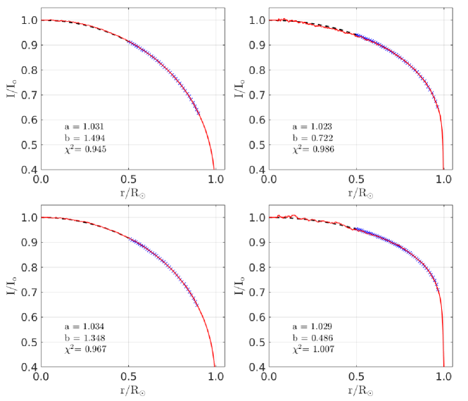
Figure 10.: Radial CLV intensity profile derived from KSO white-light (left) and H$\alpha$ (right) images. In the upper panel the images were selected during quiet Sun conditions on 1 August 2017. The lower panel shows the profiles for 22 October 2014, when a very large sunspot group was present. The red curve is the CLV profile calculated from the median intensity of the rings around Sun centre, the blue crosses correspond to the CLV functional fit to the data according to Eq. Eq:clv for $r>0.5R_{\odot}$, and the dashed line is the extrapolation of the CLV fit to $r<0.5R_{\odot}$.fig:clvwlhalph

Finally, the CLV profile fit parameters $a$ and $b$ were also studied in their evolution over complete observing days and compared to different other image parameters, such as exposure time ($exp$), the global image quadrant intensity ratio ($fpr$), the image sharpness parameter and the image quality ($Q$) from Jarolim et al. (2020). Figure fig:parquality shows as an example comparison of these parameters over about one hour of H$\alpha$ observations. As can be seen, the CLV parameters evolution during the day also delivers an assessment of the image quality. In general, values deviating from average $a$ and $b$ are related to lower image quality.

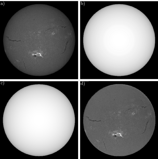
Figure 11.: KSO H$\alpha$ flare image on 22 October 2014 at 14:55:05 UT. a) Original image, b) raw CLV determined by the median intensity along rings around the solar disc centre, c) CLV_new obtained by the functional CLV fit (Eq. Eq:clv) and extrapolation for $r>0.5R_{\odot}$, and d) image divided by CLV_new. In the raw CLV map the intensity variations between the individual rings are visible, these are smoothed out in CLV_new by applying the functional fit. The contrast in image d) is constant from the disc centre to the limb.fig:correctclv

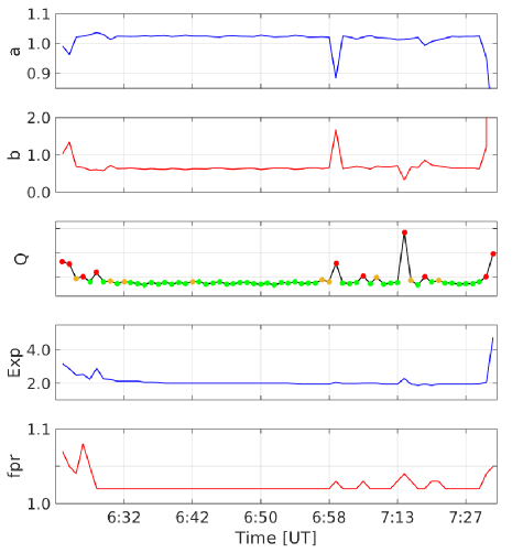
Figure 12.: Evolution of KSO image parameters during one hour of H$\alpha$ observations on 19 May 2020. From top to bottom: CLV parameters $a$ and $b$, image quality parameter from GAN ($Q$), exposure time ($exp$) and global quadrant intensity ratio ($fpr$). Deviations of the parameter $a$ and $b$ are linked to lower image quality $Q$ (i.e., green dots for quality class 1 and orange or red dots for classes 2 and 3, respectively).fig:parquality

3.4.2 Global anisotropies

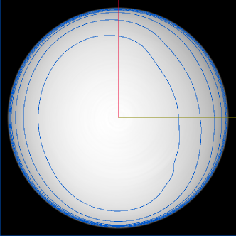
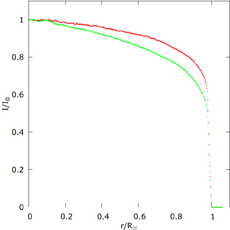
Figure 13.: Global anisotropies map derived from an H$\alpha$ image of 26 January 2021 and the corresponding normalized radial intensity profiles. Due to the optical parts in the telescope the intensity distribution in the map is not radially symmetric, which can be clearly seen in the overlaid contour lines (blue). The red and green lines correspond to the intensity profiles shown in the right panel.fig:aniso

Normally the telescope optics introduces additional intensity inhomogeneities. This can be due to dust, stray-light, filters or even shutters (a good example can be seen in Denker et al. (1999)). In order to remove also such influences the method of obtaining the CLV profile has to be adapted by replacing the median of each concentric ring with a running median. This method was first used by K. A. Burlov-Vasiljev at Kiepenheuer Institute in Freiburg, Germany. For this purpose the filter width of the running median filter applied to each concentric ring has to be set in order to neglect solar features but still detect large scale inhomogeneities. A filter width of twice the radius of each concentric ring ($\approx$ one third of the length of the ring) seems to be a choice that fullfills these criteria. The central part ($r<R_{\odot}/20$) is treated as for the CLV determination, where the median of the whole disc inside this boundary is taken. In the H$\alpha$ images at KSO there is a small intensity gradient from east to west (left to right), this can be seen in the contour lines of the anisotropy map of Figure fig:aniso. The right panel illustrates this gradient more apparently. The red profile from centre to north looks like a standard CLV profile, whereas the green profile from centre to west drops down too rapidly.

To get a widely flat image – having a uniformly distributed intensity level and everywhere almost the same image contrast – the image has to be divided by the obtained anisotropic map. Figure fig:contr shows a comparison between the original image (left) and the flat image (right). Especially features at the limb, like the small active region in the west (right), become better visible. The radial intensity profiles shown beneath the image demonstrates the flatness of the image, the higher values and the variations in the central part ($r/R_{\odot}\approx 0$) are a result of the small number of averaged pixels. The variations near $r/R_{\odot}=0.55$ are introduced by the large active region. The peak at the limb of the corrected profile is due to the roughness of the solar limb caused by seeing effects. The jump at $r/R_{\odot}>1.0$ in the intensity profile is a result of the scaling above the solar limb in order to enhance prominences.

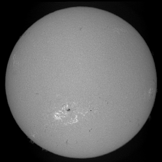
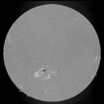
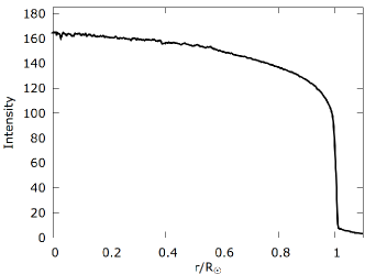
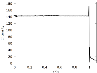
Figure 14.: H$\alpha$ images for comparison between normal contrast image (left) and high contrast image (right) divided by an anisotropy map from 28 November 2020. The radial intensity profile under each image shows that the corrected image is nearly flat after the correction. The wiggly structure near $r/R_{\odot}\approx 0$ is due to the little number of averaged pixels. The jump at the limb in the right profile is a result of the extra treatment of the scaling inside the solar disc and above the solar limb.fig:contr

3.4.3 Flat field determination

subFF

The Kuhn-Lin-Loranz (Kuhn, Lin, and Loranz, 1991) method is used to obtain a real flat field, that also includes smaller intensity variations, like dust particles: This method is based on the assumption that the Sun does not change its appearance within a few seconds. A set of Sun images shifted on the CCD is used to calculate the intensity for each CCD pixel. The more images are used and the less the Sun changes, good seeing conditions are a premise, the better the flat field becomes. A drawback of this method is, that this procedure needs manual interaction, and cannot be performed very often as it interrupts the patrol observations.

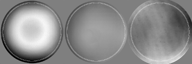
Figure 15.: Flat field frames for Ca ii K (left, 9 April 2021), white-light (centre, 9 May 2012) and H$\alpha$ (right, 3 June 2021) telescopes. The contrast is strongly enhanced to see the inhomogeneities better. The white rings represent the limits of the solar disc size in aphelion and perihelion. Missing values and regions far above the solar limb are set to 1. The enhanced intensity in a concentric ring at about $R_{\odot}/3$ in the Ca ii K flat field is due to the filter. The interference pattern in H$\alpha$ is most likely produced within the Lyot filter.fig:ff

At KSO for such a flat field one centre image plus 28 shifted images are taken. The shifted images are on three concentric rings, four images with a shift of 115 pixel ($\approx R_{\odot}/8$), 8 images with a shift of 230 pixel and 16 images with a shift of 345 pixel. The exposure time is set to a fixed value and the duration of the whole procedure is kept as short as possible in order to have almost the ”same” Sun for all images. Taking the full frameset takes about four minutes, most of the time is used for moving the telescope. Starting with 2021, flat field frames are produced for all telescopes (H$\alpha$, Ca ii K and white-light), when the seeing conditions are exceptionally good or when there are any changes in the telescope setup. Figure fig:ff shows an example for flat field frames of all three telescopes. For Ca ii K images the interpolation of the CLV according to Eq. Eq:clv does not work properly. The reason for this is the intensity distribution of the flat field, which seems to be produced mainly by the Ca ii K filter. This flat field shows a ring-like intensity enhancement at $R_{\odot}/3$, the central intensity is even lower than in this ring. The white-light flat field (centre panel of Figure fig:ff) shows a relatively uniformly distribution, some very small dust particles are visible. The H$\alpha$ flat field (right panel of Figure fig:ff) is dominated by three features: The interference pattern (dark and bright bands) are very likely produced by the Lyot filter, additionally there is a global intensity gradient from the centre to the left and to the right and there are some dust particles. We have to note that the contrast in these flat field frames was strongly enhanced to make all these features visible, the intensity difference within the solar disc is about two percent. The horizontal and vertical structures are an artefact due to the image motion caused by atmospheric conditions, which should be theoretically zero for applying the Kuhn-Lin-Loranz method. Also the small scale structures are a result of the seeing. To get rid of these artefacts a really exceptionally good seeing is necessary for getting a good flat field with this method. The most important application for such a flat field map is to detect dust particles on the optical parts and to see the influences of the telescope optics on the camera image. Applying such a flat field on the raw image can only be done after some smoothing steps in order to get rid of the fine structures introduced by the seeing.

4 Data Provision

4.1 KSO data archive

subArch

The image archive of KSO as presented in Pötzi, Hirtenfellner-Polanec, and Temmer (2013) underwent a number of changes and updates in the recent years. The most important improvement is the instant of time of availability of the data in the archive. Whereas the archive was normally updated at the end of an observing day, it is now updated continuously in quasi real-time simultaneously to the observations. Every minute, for each telescope one newly recorded image is transferred to the archive. As there are differences in the image cadence (10 images per minute for H$\alpha$ and Ca ii K and 3 images per minute for white-light), additional recorded images are transferred to the archive after the observing day. The number of additional images to be transferred is selected depending on camera type and solar activity. Normally three chromospheric (H$\alpha$ and Ca ii K) images per minute are stored and one photospheric (white-light). In case of large solar flares (defined of GOES class $\geq$ M1 or optical flare importance class $\geq 1$) all images of good and fair quality recorded during flare activity are transferred to the archive.

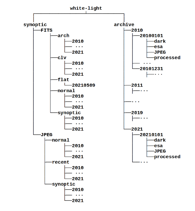
Figure 16.: The data path for the full white-light data set. A data set of one daily processed image is in the synoptic path, the whole daily data is located in the archive path.fig:paths

The data archive consists of the synoptic and the main archive branch (see Figurefig:paths). The synoptic archive consists of one higher level image data set for each observing day. The main archive holds all the observed raw images as FITS files and their corresponding processed JPEG quick look files. The data hierarchy in the synoptic branch goes from data type to yearly directories. In the main archive the data are stored in yearly directories containing the folders for each observing day. All archive data are mirrored in a local archive simultaneously. With a delay of a few hours, the data are also transferred to a mirror archive located physically at the University of Graz (Figure fig:grazmirr), which provides a higher bandwidth for faster data transfer. The archive can be accessed via following ways:

• KSO archive webpage http://cesar.kso.ac.at

• KSO ftp ftp://ftp.kso.ac.at, instructions how to access the server can be found on http://cesar.kso.ac.at/main/ftp.php

• for the transfer of large data sets we suggest the use of the mirror http://kanzelhohe.uni-graz.at (Figure fig:grazmirr) as it guarantees faster download rates.

• ESA SSA Spaceweather portal https://swe.ssa.esa.int, registration is necessary to access this data.

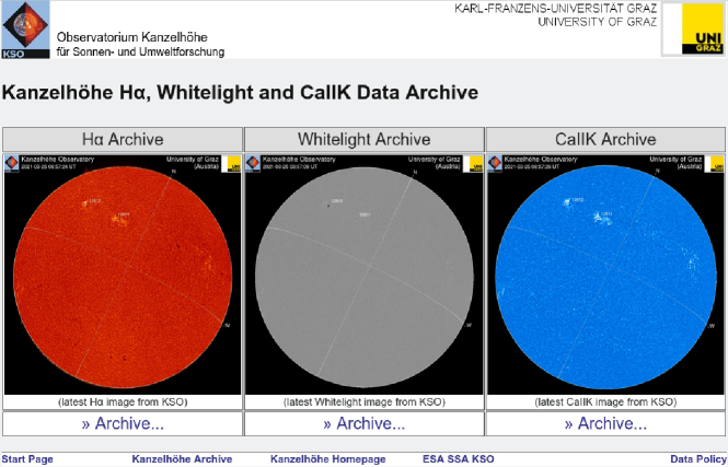
Figure 17.: The mirror archive located physically at University of Graz is operated for fast data access. In case of large data transfers this archive should be favoured.fig:grazmirr

4.1.1 Synoptic archive data products

The directory structure for the synoptic archive shown in Figure fig:paths (left) consists of a FITS and JPEG path for each camera containing a set of files for each observing day. The image is selected manually by the observer and set of various images and profiles is processed for displaying on the observatory website. These data are for a quick daily overview of the situation on the Sun.

• kanz_[type]_fi_[yyyymmdd]_[HHMMSS].fts.gz

  • the raw selected image with updated FITS header

  • located in FITS/arch/[yyyy]

  • example:kanz_caiik_fi_20210425_060742.fts.gz

• kanz_[type]_fq_[yyyymmdd]_[HHMMSS].fts.gz

  • the CLV intensity profile

  • located in FITS/clv/[yyyy]

  • example:kanz_halph_fq_20150107_120351.fts.gz

• kanz_[type]_fc_[yyyymmdd]_[HHMMSS].fts.gz

  • a high contrast image i.e. global anisotropies are corrected and the solar disc is centred.

  • located in FITS/normal/[yyyy]

  • example:kanz_caiik_fc_20210425_060742.fts.gz

• kanz_[type]_ff_[yyyymmdd].fts.gz

  • the flat field map normalized to 1.0 and the individual raw files used to generate this flat field map.

  • located in FITS/flat/[yyyymmdd]

  • example:kanz_caiik_ff_20210409.fts.gz

• kanz_[type]_fd_[yyyymmdd]_[HHMMSS].fts.gz

  • a normal contrast image with centred solar disc.

  • located in FITS/synoptic/[yyyy]

  • example:kanz_bband_fd_20151227_0847.fts.gz

• kanz_[type]_fc_[yyyymmdd]_[HHMMSS].jpg

  • a high contrast image i.e. global anisotropies are corrected, the solar disc is centred, a heliographic grid is overlaid, the image is rotated to North up and annotated.

  • located in JPEG/normal/[yyyy]

  • example:kanz_halph_fc_20210425_060748.jpg

• kanz_[type]_fc_[yyyymmdd]_[HHMMSS].icon.jpg

  • an icon of the high contrast image.

  • located in JPEG/recent/[yyyy]

  • example: kanz_halph_fi_20210425_060748.icon.jpg

• kanz_[type]_fd_[yyyymmdd]_[HHMMSS].jpg

  • a normal contrast image i.e. the solar disc is centred, an unsharp masking is applied for little contrast enhancement, the image is rotated to North up and annotated.

  • located in JPEG/synoptic/[yyyy]

  • example: kanz_bband_fd_20151227_0847.jpg

Where [type] is one of halph (= H$\alpha$), bband (= white-light) or caiik (=Ca ii K) and [yyyymmdd]_[HHMMSS] is the date and time of image capture.

4.1.2 Main archive data products

The main archive contains all images of quality classes 1 and 2 in raw format (only FITS header updated) and as quick look JPEG files in various types as described below. The cadence of the data is three images per minute for H$\alpha$ and Ca ii K observations and one image per minute for white-light. In case of flares this cadence is increased to 10 images per minute for chromospheric observations. On a day with good observing conditions and a very active Sun up to 10 000 images can be stored in the archive.

• kanz_[type]_fi_[yyyymmdd]_[HHMMSS].fts.gz

  • located in [yyyymmdd]/processed

  • raw image files, only the FITS header is updated to its full version (see Appendix Table tbl:FITS)

  • example: kanz_bband_fi_20170906_085054.fts.gz white-light image of 6 September 2017

• kanz_[type]_fi_[yyyymmdd]_[HHMMSS].jpg

  • located in [yyyymmdd]/JPEG

  • greyscale quick look jpg files with annotation and logos and unsharp mask applied for better contrast.

  • example: kanz_bband_fi_20170906_085054.jpg white-light image of 6 September 2017

• dc[yyyymmdd]_[HHMMSS].fts.gz

  • located in [yyyymmdd]/dark

  • dark current images, normally two per day, at the beginning and at the end of an observation day. The dark current is taken, when objective lens is covered with its protection cap.

  • example: dc20180127_073644.FTS.gz for white-light camera of 27 January 2018

• [yyyymmdd]_[HHMMSS].jpg

  • located in [yyyymmdd]/esa

  • coloured JPEG files with logos, annotation and heliographic grid and unsharp masking for contrast enhancement (not existing for Ca ii K).

  • example: 20210422_060537.jpg H$\alpha$ image of 22 April 2021

• [yyyymmdd]_[HHMMSS]_fc.jpg

  • located in [yyyymmdd]/esa

  • coloured jpg files with logos, annotation and heliographic grid and corrected global anisotropies (not existing for Ca ii K).

  • example:20210422_060537_fc.jpg H$\alpha$ image of 22 April 2021

• [yyyymmdd].avi

  • located in [yyyymmdd]/

  • a daily overview movie generated from greyscale JPEG files.

  • example: 20201107.avi Ca ii K movie for 7 November 2020

• [yyyymmdd]_[HHMM]_[IdId].html

  • located in [yyyymmdd]/movie

  • javascript movies of automatically detected flares. These movies are only produced for H$\alpha$ flares.

  • example: 20170905_0745_0003.html movie of importance class 1B from 5 September 2017

• [yyyymmdd]_movie.html

  • located in [yyyymmdd]/

  • a daily javascript movie of coloured JPEG files. This movie is only produced for H$\alpha$.

  • example: 20140127_movie.html H$\alpha$ movie for 27 January 2014

[IdId] denotes a 4-digit internal number for identifying the flare region in the automatic flare detection system number. The colours in the coloured images are red for H$\alpha$ and grey for white-light. The sizes of the jpg images are reduced to 1024$\times$1024 pixels.

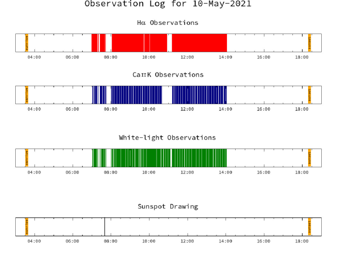
Figure 18.: Graphical observation log for 10 May 2021. For each observed image of quality class 1 or 2 a line is drawn. Clouds at around 8:00 UT and 11:00 UT interrupted the observations.fig:obslog

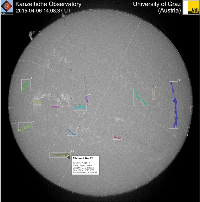
Figure 19.: H$\alpha$ sensitive map of 6 April 2015: an H$\alpha$ image is overlaid with automatically detected filaments. When the mouse pointer is moved over a filament additional information, like position and size, are shown.fig:fil

4.1.3 Derived higher level data products

The following higher level data products that are derived from the above data are also available:

• Daily graphical observation logs are created after each observing day to present a quick overview with time marks for each archived image for all cameras (see Figure fig:obslog). These are created after each observing day and made available via the KSO archive webpage.

• Sensitive filament maps are generated from the filament data produced by the automatic flare and filament detection system (Pötzi et al., 2015). These filament data are combined to hourly sensitive maps (Figure fig:fil), where H$\alpha$ images are overlaid with detected filaments. When the mouse pointer is moved over a filament, position, size and area information is shown. Via the ESA SSA space weather portal also data from the database can be obtained in a JSON format.

• Flare data and movies which are also produced by the automatic flare detection system are available within the ESA SSA Space weather portal and the KSO archive webpage. Each detected H$\alpha$ flare is characterized by start time, peak time, end time and flare importance class. Each flare is linked to its corresponding interactive javascript movie (described in the main archive products above).

• In the H$\alpha$ light curves a plot of the brightest pixel in each H$\alpha$ image is overlaid by GOES full-Sun SXR flux profiles. The GOES data is obtained from NOAA/SWPC (National Oceanic and Atmospheric Administration/Space Weather Prediction Center), using the long wavelength band (1.0 – 8.0 Å). Additionally automatically detected flares together with their H$\alpha$ importance class are annotated in the plot (see Figure fig:lightc).

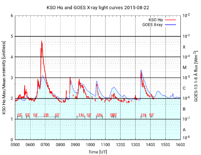
Figure 20.: The mean intensity of the four brightest pixels in each H$\alpha$ image normalized by the mean value of the full solar disc are plotted in red along with the GOES 1-8 Å X-ray flux in blue. During flares both curves should show a local peak. The results of the automatic real-time flare detection (flare start to end; H$\alpha$ flare importance class) are plotted in the bottom.fig:lightc

4.1.4 Other data products and former data products

The links to the different data products can be found in Tab. tbl:data.

• Prominence images: Once a day, when there are no thin clouds, a set of H$\alpha$ images is taken with the exposure times up to 50 ms. As a result the solar disc is completely saturated, but prominences above the limb become better visible. Due to telescope limitations, prominences can only be viewed up to 1.13 $R_{\odot}$. This data are used as complementary data to fill gaps of the Lomnický Štít prominence catalogue (Rybák et al., 2011).

• The daily sunspot drawings are scanned immediately and available on the KSO archive webpage together with the derived sunspot relative numbers. This is the longest data set of KSO reaching back to 1944.

• H$\alpha$ photographic film data between 1973 and 2000 were scanned (Pötzi, 2007) and are available as full FITS and JPEG archive.

• H$\alpha$ CCD data observed with the former cameras (see Tab.tbl:patrol) with less resolution and less image depth are also available as synoptic and full data archive.

• White-light photographic images, of which normally three exposures on 13$\times$18 cm flat film were taken per day between 1989 and 2007, have been scanned and processed (Pötzi, 2010). The archive consists of the raw FITS files and JPEG images with overlaid heliographic grid.

• NaD intensitygrams (5890 Å), dopplergrams and magnetograms of the Magneto Optical Filter (MOF) as described in Cacciani et al. (1999) (about the data reduction see Moretti and MOF Development Group, 2000). In the synoptic archive intensitygrams and magnetograms are available, the main archive consists of dopplergrams, intensitygrams and magnetograms. The data is only available from June 2000 to July 2002.

Table 2.: Summary of the links to KSO data products. (1 - web interface, 2 - to access the ESA-SSA data a free of charge registration is necessary.tbl:data

data	link
H$\alpha$ synoptic1	http://cesar.kso.ac.at/synoptic/ha_years.php
H$\alpha$ 4 MPix 12bit archive	http://cesar.kso.ac.at/halpha3a
Ca ii K synoptic1	http://cesar.kso.ac.at/synoptic/caii_years.php
Ca ii K  archive	http://cesar.kso.ac.at/caiia
white-light synoptic1	http://cesar.kso.ac.at/synoptic/con_years.php
white-light archive	http://cesar.kso.ac.at/phokada
graphical observation logs1	http://cesar.kso.ac.at/kh_obslog/kh_obslog_query.php
prominence images1	http://cesar.kso.ac.at/synoptic/kor_years.php
sunspot drawings1	http://cesar.kso.ac.at/synoptic/draw_years.php
sunspot numbers1	http://cesar.kso.ac.at/synoptic/num_years.php
H$\alpha$ scanned film archive	http://cesar.kso.ac.at/hafilma
H$\alpha$ 1 MPix 8bit archive	http://cesar.kso.ac.at/halpha1a
H$\alpha$ 1 MPix 10bit archive	http://cesar.kso.ac.at/halpha2a
MOF archive + synoptic	http://cesar.kso.ac.at/mof
filament data1	http://cesar.kso.ac.at/sn_iv/filaments.php
H$\alpha$ light curves ESA-SSA	http://cesar.kso.ac.at/flares/intensity
filament data ESA-SSA2	https://swe.ssa.esa.int/web/guest/kso-S107f-federated
flare data ESA-SSA2	https://swe.ssa.esa.int/web/guest/kso-S107c-federated
H$\alpha$ light curves ESA-SSA2	https://swe.ssa.esa.int/web/guest/kso-S107g-federated

4.2 KSO Database

subDB

The database is located on Kanzelhöhe Electronic Archive System (KEAS, Otruba and Egarter, 2007) and holds all compulsory information about the images. The database is updated with every image transferred to the archive. E.g., the following data is stored for each image:

• the camera brand and CCD size

• the filter brand, wavelength and FWHM

• date and time of image acquisition

• exposure time in milliseconds

• image quality (1-3)

• centre coordinates $x$ and $y$ of the solar disc in pixel

• radius of the solar disc in pixel

• image size in $x$ and $y$ direction

• filesize in bytes of the FITS file

• filename of FITS file including path as accessible via http

• available JPEG file types

The database has nearly 5 million entries of solar images. All of them are accessible through the archive. Most entries are H$\alpha$ images (about 3.5 million). For each entry there exists a FITS file and at least one JPEG file, in case of good quality additionally a coloured JPEG file and a coloured high contrast JPEG file are available. The image database can be accessed via the archive page directly http://cesar.kso.ac.at/catalogue/search_obj.php (left side “Database Search”). Figure fig:database shows the query page and the result of this query beneath.

For scripts and automatized searches following APIs are available:
http://cesar.kso.ac.at/database/get_halpha.php?from=datetime&to=datetime
http://cesar.kso.ac.at/database/get_wl.php?from=datetime&to=datetime
http://cesar.kso.ac.at/database/get_caii.php?from=datetime&to=datetime
The parameters are the following:

• from: start date and time in the format yyyy-mm-ddTHH:MM:SS.

• to: end date and time in the format yyyy-mm-ddTHH:MM:SS.

• ftype: (optional) can be one of all, jpeg, fits.

• color: (optional) set to 1 if coloured normal contrast and high contrast (global anisotropies corrected) images are wanted.

• html: (optional) set to 1 if html output is requested, the default output is a list with comma separated entries (csv).

• qual: (optional) select the highest quality level to select, default is 3 i.e. 1,2 and 3 are selected.

• filesize: (optional) set to 1 if the filesize in bytes should be returned, this can be of interest for estimating the download time.

E.g., to get all H$\alpha$ image entries between 08:00:00 UT and 10:00:00 UT for 23 May 2021 including file sizes and coloured JPEGs the API looks like this:
http://cesar.kso.ac.at/database/get_halpha.php?from=2021-05-23T08:00:00&to=2021-05-23T10:00:00&html=1 This gives in principle the same output as shown in the result in Figure fig:database. These APIs are also used, e.g., to populate the KSO data of the Virtual Solar Observatory (VSO, Davey (2014)), where all entries of our database are replicated back to 1973.

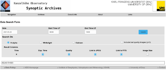
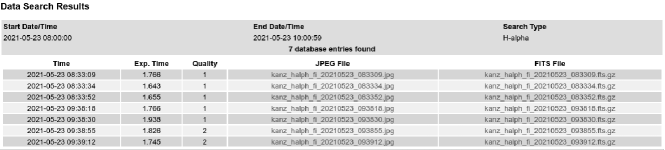
Figure 21.: Example for the database query interface and result: Above the database query for H$\alpha$ images between 08:00 UT and 10:00 UT for 23 May 2021. Below the result of this query, the file entries are links that can be viewed directly.fig:database

5 Conclusion

This paper gives an overview of the data processing pipeline, the data archive and the data products of the KSO solar observations. The Kanzelhöhe data pipeline could act as an example of how to process data fast and effectively. The time from data acquisition to data provision is outstanding low, it can really be called “near real-time” data. This fast processing is due to the three separated tasks – acquisition, processing and provision – running on independent servers. The processing part, e.g., is even implemented on two workstations to reduce the workload, but can in case of a hardware failure run also on one workstation alone. The data are never stored locally on camera controllers, all data beginning from data acquisition to processed data and temporary data are on network attached storages (NAS) that are accessible from all workstations. This separation of tasks on different workstations has the advantage that all steps can run in parallel, each step is just waiting for data produced by the previous step. The second important point is an almost immediate and easy access to the observed data. For this purpose data in lower cadence (one image per minute) is transferred immediately after processing to the archive and made accessible via the database. At the end of an observing day the archive and the database are filled up with the rest of the data. The data can then be retrieved via web interfaces or ftp access. Database queries can be done directly over the archive web page or automatized via scripts using the described APIs.

Both, the fast data processing and the fast data availability, can only exist due to the automatized data processing pipeline. The basis for this pipeline is the quality determination of the incoming data, that decides whether an image is dismissed or further processed. The provided data products serve as direct input to automated solar feature detection algorithms and allow to study the Sun in high-resolution and high-cadence.

Appendix A Camera specifications

camera

The cameras are equipped with a ON Semiconductor KAI-4021 monochrome CCD sensor. The number of active pixels is 2048$\times$2048, each with a size of $7.4\,\mu\rm{m}\times 7.4\,\mu\rm{m}$, resulting in a total sensor size of $15.1\,\rm{mm}\times 15.1\,\rm{mm}$. The peak quantum efficiency is 55% at 475 nm, i.e. the quantum efficiency for Ca ii K (393 nm) is 45%, for white-light (545 nm) $\approx$50%, and for H$\alpha$ (656 nm) 30%. The maximum data rate is 40 MHz, which limits the frame rate to about 9 images per second in 12bit mode. This frame rate is reduced to 7 frames per second in our software when frame selection is active. The sensor is a interline progressive scan CCD, which reads out all pixels simultaneously. The number of dead pixels is zero for the H$\alpha$ camera, one for the white-light camera and three for the Ca ii K camera. These dead pixels are replaced by the average intensity of the two neighbouring horizontal pixels. Detailed information about the image sensor can be found at https://www.onsemi.com/pdf/datasheet/kai-4021-d.pdf.

Appendix B Quality parameters

qualparam

The parameters for determination of image quality of
H$\alpha$ filtergrams:

• high exposure times ($exp\geq 18$ ms): quality class 3

• rms of solar radius determination $>5$ pixel: quality class 3

• global quadrant intensity ratio $>1.08$: quality class 3

• $exp$ $>5$ ms and rms of solar radius $>$ 3: quality class 3

• image sharpness $<50$: quality class 2

• image sharpness $<25$: quality class 3

• mean intensity in AOI $\leq 400$ or $\geq 1200$ counts: quality class 3

Ca ii K filtergrams:

• high exposure times ($exp\geq 25$ ms): quality class 3

• rms of solar radius determination $>4$ pixel: quality class 3

• global quadrant intensity ratio $>1.10$: quality class 3

• $exp$ $>15$ ms and rms of solar radius $>$ 3: quality class 3

• image sharpness $<22.5$: quality class 2

• image sharpness $<14$: quality class 3

• mean intensity in AOI $\leq 500$ or $\geq 1200$ counts: quality class 3

white-light images:

• high exposure times ($exp\geq 12$ ms): quality class 3

• rms of solar radius determination $>3$ pixel: quality class 3

• global quadrant intensity ratio $>1.10$: quality class 3

• $exp$ $>8$ ms and rms of solar radius $>$ 2: quality class 3

• image sharpness $<8$: quality class 2

• image sharpness $<5$: quality class 3

• mean intensity in AOI $\leq 500$ or $\geq 2500$ counts: quality class 3

The contrast in white-light images seems to be more sensitive to clouds, therefore the limit for the exposure time setting is here very restrictive. The radius detection is most accurate for white-light as the photosphere shows a very sharp intensity drop at the limb. This explains the higher tolerance for the rms of the radius determination in H$\alpha$ as compared to white-light. The granulation in white-light images disappears immediately when the image is smoothed. Therefore the limit for the image sharpness is set very low, i.e., this parameter is not very suitable for this image type.

Appendix C FITS header

FITS

Table 3.: The FITS keywords for an H$\alpha$ image, Ca ii K or white-light have the same keywords. Here an example for white-light from 13 January 2021 at 08:00:39 UT.tbl:FITS

0	SIMPLE	= T	/ file does conform to FITS standard
1	BITPIX	= 16	/ number of bits per data pixel
2	NAXIS	= 2	/ number of data axes
3	NAXIS1	= 2048
4	NAXIS2	= 2048
5	EXTEND	= ’F ’	/ no extensions
6	FILENAME	= ’kanz_halph_fi_20210113_080039.fts.gz’
7	DATE	= ’2021-01-13T08:00:42’	/ file creation date (YYYY-MM-DDThh:mm:ss UT)
8	DATE-OBS	= ’2021-01-13T08:00:39’	/ Date of observation
9	DATE-BEG	= ’2021-01-13T08:00:39’	/ Date of observation
10	TIMESYS	= ’UTC ’
11	OBSVTRY	= ’Kanzelhoehe Observatory’
12	TELESCOP	= ’KHPI ’
13	INSTRUME	= ’HA2 ’
14	DETECTOR	= ’TM4200-6’	/ Camera Type
15	OBJECT	= ’Full Sun’
16	FILTER	= ’Zeiss Lyot Halpha’
17	WAVELNTH	= 6562.8	/ [ANG], FWHM=0.7 [ANG]
18	WAVEMIN	= 6562.45
19	WAVEMAX	= 6563.15
20	EXP_TIME	= 2.058	/ Exposure Time [ms]
21	XPOSURE	= 0.002058	/ [s]
22	BSCALE	= 1	/ default scaling factor
23	BZERO	= 32768	/ offset data range to that of unsigned short
24	BUNIT	= ’CCD COUNTS’
25	DATAMIN	= 0
26	DATAMEAN	= 539
27	DATAMAX	= 657
28	CTYPE1	= ’SOLAR_X ’
29	CTYPE2	= ’SOLAR_Y ’
30	CUNIT1	= ’arcsec ’
31	CUNIT2	= ’arcsec ’
32	CRPIX1	= 1024.5	/ [pix]
33	CRPIX2	= 1024.5	/ [pix]
34	CDELT1	= 1.026318	/ [arcsec/pix]
35	CDELT2	= 1.026318	/ [arcsec/pix]
36	CRVAL1	= 1.838296
37	CRVAL2	= 1.425863
38	ANGLE	= -4.725313	/ [deg]
39	CROTA1	= 4.725313	/ [deg]
40	CENTER_X	= 1022.709	/ [pix]
41	CENTER_Y	= 1023.111	/ [pix]
42	SOLAR_R	= 955.2872	/ [pix]
43	RSUN_REF	= 6.9938E+08	/ [m]
44	RSUN_ARC	= 980.4283	/ [arcsec]
45	SOLAR_P0	= -3.970842	/ [deg]
46	SOLAR_B0	= -4.385699	/ [deg]
47	CAR_ROT	= 2239
48	QUALITY	= 1	/ image quality [1-3]
49	OBS_TYPE	= ’HALPH ’
50	OBS_PROG	= ’HALPHA PATROL’
51	TYPE-DP	= ’ARCHIVE ’	/ Data Processing Type
52	EXP_MODE	= 0	/ Exp. Mode (0=auto,1=dbl,2=fix,3=both)
53	PRE_INT	= 600	/ Preselected PixInt in AOI
54	A_O_INT	= ’800,900,800,1100’	/ Rect. for PixInt [X0,Y0,X1,Y1]
55	ORIGIN	= ’KANZELHOEHE OBSERVATORY, A-9521 TREFFEN, AUSTRIA’
56	COMMENT Orientation: N up, W right, first pix is left bottom
57	HISTORY No intensity processing applied
58	END

The FITS header keywords (see Tab. tbl:FITS) used at KSO are mostly in accordance with the Metadata Definition for Solar Orbiter Science Data published by ESA (De Groof, Walsh, and Williams, 2019). Most of the keywords are clear, but some need an additional explanation and sevral keywords have the same value or meaning are included for compatibility reasons with older software.

• Date and time of image capture.

• Date and time of FITS creation.

• both are the exposure times but the first is in milliseconds and the latter in seconds.

• the angular aperture of pixels in arcsec, this angle refers to the viewing angle and not to heliographic coordinates

• the value of CRPIX1 and CRPIX2 in arcsec, it is for the horizontal coordinate (CRPIX1-CENTER_X)$\times$CRDELT1.

• The inclination of solar north clockwise and counter clockwise, it is the sum of SOLAR_P0 and the camera tilt angle.

• The reference radius of the Sun in meters based on the IAU (Prša et al., 2016) value for the photosphere and for the chromosphere transit measurements in H$\alpha$ from KSO were taken, resulting in a thickness of 3 600 km.

• The actual diameter of the Sun in arcsec depending on the distance of the sun and RSUN_REF.

• The requested intensity in the AOI for the frame selection procedure which defines the exposure time.

• the coordinates of the AOI rectangle.

Acknowledgments

This research has received financial support from the European Union’s Horizon 2020 research and innovation program under grant agreement No. 824135 (SOLARNET).

Disclosure of Potential Conflicts of Interests

The authors declare that they have no conflicts of interest.

References

- Aggarwal et al. (2018) Aggarwal, A., Schanche, N., Reeves, K.K., Kempton, D., Angryk, R.: 2018, Prediction of Solar Eruptions Using Filament Metadata. ApJS 236, 15. DOI. ADS.
- Baranyi, Győri, and Ludmány (2016) Baranyi, T., Győri, L., Ludmány, A.: 2016, On-line Tools for Solar Data Compiled at the Debrecen Observatory and Their Extensions with the Greenwich Sunspot Data. Sol. Phys. 291, 3081. DOI. ADS.
- Cacciani et al. (1999) Cacciani, A., Moretti, P.F., Messerotti, M., Hanslmeier, A., Otruba, W., Pettauer, T.V.: 1999, In: Hanslmeier, A., Messerotti, M. (eds.) The Magneto-Optical Filter at Kanzelhöhe 239, 271. DOI. ADS.
- Chatterjee et al. (2020) Chatterjee, S., Hegde, M., Banerjee, D., Ravindra, B., McIntosh, S.W.: 2020, Time-Latitude Distribution of Prominences for 10 Solar Cycles: A Study Using Kodaikanal, Meudon, and Kanzelhohe Data. Earth and Space Science 7, e00666. DOI. ADS.
- Chatzistergos et al. (2017) Chatzistergos, T., Usoskin, I.G., Kovaltsov, G.A., Krivova, N.A., Solanki, S.K.: 2017, New reconstruction of the sunspot group numbers since 1739 using direct calibration and “backbone” methods. A&A 602, A69. DOI. ADS.
- Chatzistergos et al. (2020) Chatzistergos, T., Ermolli, I., Krivova, N.A., Solanki, S.K., Banerjee, D., Barata, T., Belik, M., Gafeira, R., Garcia, A., Hanaoka, Y., Hegde, M., Klimeš, J., Korokhin, V.V., Lourenço, A., Malherbe, J.-M., Marchenko, G.P., Peixinho, N., Sakurai, T., Tlatov, A.G.: 2020, Analysis of full-disc Ca II K spectroheliograms. III. Plage area composite series covering 1892-2019. A&A 639, A88. DOI. ADS.
- Chowdhury et al. (2019) Chowdhury, P., Kilcik, A., Yurchyshyn, V., Obridko, V.N., Rozelot, J.P.: 2019, Analysis of the Hemispheric Sunspot Number Time Series for the Solar Cycles 18 to 24. Sol. Phys. 294, 142. DOI. ADS.
- Clette and Lefèvre (2016) Clette, F., Lefèvre, L.: 2016, The New Sunspot Number: Assembling All Corrections. Sol. Phys. 291, 2629. DOI. ADS.
- Clette et al. (2014) Clette, F., Svalgaard, L., Vaquero, J.M., Cliver, E.W.: 2014, Revisiting the Sunspot Number. A 400-Year Perspective on the Solar Cycle. Space Sci. Rev. 186, 35. DOI. ADS.
- Comper (1958) Comper, W.: 1958, Die eruptive Protuberanz vom 16. Dezember 1956. Mit 9 Textabbildungen. ZAp 45, 83. ADS.
- Comper and Kern (1957) Comper, W., Kern, R.: 1957, Die Eruption (Flare) und der Protuberanzenaufstieg vom 4. Juni 1956. Mit 4 Textabbildungen. ZAp 43, 20. ADS.
- Davey (2014) Davey, A.R.: 2014, The Virtual Solar Observatory: New Data, Big Data and Better Queries. In: American Astronomical Society Meeting Abstracts #224, American Astronomical Society Meeting Abstracts 224, 218.46. ADS.
- De Groof, Walsh, and Williams (2019) De Groof, A., Walsh, A., Williams, D.: 2019, Metadata definition for solar orbiter science data, ESA. https://issues.cosmos.esa.int/solarorbiterwiki/display/SOSP/Metadata+Definition+for+Solar+Orbiter+Science+Data.
- Dellinger (1935) Dellinger, J.H.: 1935, A New Cosmic Phenomenon. Science 82, 351. DOI. ADS.
- Denker et al. (1999) Denker, C., Johannesson, A., Marquette, W., Goode, P.R., Wang, H., Zirin, H.: 1999, Synoptic H Full-Disk Observations of the Sun from BigBear Solar Observatory - I. Instrumentation, Image Processing, Data Products, and First Results. Sol. Phys. 184, 87. DOI. ADS.
- Filippov (2013) Filippov, B.: 2013, A Filament Eruption on 2010 October 21 from Three Viewpoints. ApJ 773, 10. DOI. ADS.
- Hanslmeier and Lustig (1986) Hanslmeier, A., Lustig, G.: 1986, Meridional motions of sunspots from 1947.9-1985.0. I - Latitude drift at the different solar-cycles. A&A 154, 227. ADS.
- Hinterreiter et al. (2018) Hinterreiter, J., Veronig, A.M., Thalmann, J.K., Tschernitz, J., Pötzi, W.: 2018, Statistical Properties of Ribbon Evolution and Reconnection Electric Fields in Eruptive and Confined Flares. Sol. Phys. 293, 38. DOI. ADS.
- Hirtenfellner-Polanec et al. (2011) Hirtenfellner-Polanec, W., Temmer, M., Pötzi, W., Freislich, H., Veronig, A.M., Hanslmeier, A.: 2011, Implementation of a Calcium telescope at Kanzelhöhe Observatory (KSO). Central European Astrophysical Bulletin 35, 205. ADS.
- Jarolim et al. (2020) Jarolim, R., Veronig, A.M., Pötzi, W., Podladchikova, T.: 2020, Image-quality assessment for full-disk solar observations with generative adversarial networks. A&A 643, A72. DOI. ADS.
- Joshi et al. (2017) Joshi, B., Kushwaha, U., Veronig, A.M., Dhara, S.K., Shanmugaraju, A., Moon, Y.-J.: 2017, Formation and Eruption of a Flux Rope from the Sigmoid Active Region NOAA 11719 and Associated M6.5 Flare: A Multi-wavelength Study. ApJ 834, 42. DOI. ADS.
- Jungmeier (2017) Jungmeier, G.: 2017, Die Überwachung der Sonne: Die frühen Jahre des Observatoriums Kanzelhöhe, Unipress Graz, Graz, 152.
- Kuhn, Lin, and Loranz (1991) Kuhn, J.R., Lin, H., Loranz, D.: 1991, Gain calibrating NonUniform Image-Array Data Using Only the Image Data. PASP 103, 1097. DOI. ADS.
- Kuiper (1946) Kuiper, G.P.: 1946, German astronomy during the war. Popular Astronomy 54, 263. ADS.
- Lustig and Hanslmeier (1987) Lustig, G., Hanslmeier, A.: 1987, Meridional motions of sunspots from 1947.9 to 1985.0. II - Latitude motions dependent on SPOT type and phase of the activity cycle. A&A 172, 332. ADS.
- Maričić et al. (2004) Maričić, D., Vršnak, B., Stanger, A.L., Veronig, A.: 2004, Coronal Mass Ejection of 15 May 2001: I. Evolution of Morphological Features of the Eruption. Sol. Phys. 225, 337. DOI. ADS.
- Miklenic et al. (2007) Miklenic, C.H., Veronig, A.M., Vršnak, B., Hanslmeier, A.: 2007, Reconnection and energy release rates in a two-ribbon flare. A&A 461, 697. DOI. ADS.
- Moretti and MOF Development Group (2000) Moretti, P.F., MOF Development Group: 2000, Dopplergram Calibration. Sol. Phys. 196, 51. DOI. ADS.
- Möstl et al. (2009) Möstl, C., Farrugia, C.J., Miklenic, C., Temmer, M., Galvin, A.B., Luhmann, J.G., Kilpua, E.K.J., Leitner, M., Nieves-Chinchilla, T., Veronig, A., Biernat, H.K.: 2009, Multispacecraft recovery of a magnetic cloud and its origin from magnetic reconnection on the Sun. Journal of Geophysical Research (Space Physics) 114, A04102. DOI. ADS.
- Otruba and Egarter (2007) Otruba, W., Egarter, W.: 2007, KEAS::Grid. Central European Astrophysical Bulletin 31, 321. ADS.
- Otruba and Pötzi (2003) Otruba, W., Pötzi, W.: 2003, The new high-speed H imaging system at Kanzelhöhe Solar Observatory. Hvar Obs. Bull. 27, 189. ADS.
- Otruba, Freislich, and Hanslmeier (2008) Otruba, W., Freislich, H., Hanslmeier, A.: 2008, Kanzelhöhe Photosphere Telescope (KPT). Cent. Eur. Astrophys. Bull. 32, 1. ADS.
- Pettauer (1990) Pettauer, T.: 1990, The Kanzelhöhe photoheliograph. Publications of Debrecen Heliophysical Observatory 7, 62. ADS.
- Pohjolainen et al. (2001) Pohjolainen, S., Maia, D., Pick, M., Vilmer, N., Khan, J.I., Otruba, W., Warmuth, A., Benz, A., Alissandrakis, C., Thompson, B.J.: 2001, On-the-Disk Development of the Halo Coronal Mass Ejection on 1998 May 2. ApJ 556, 421. DOI. ADS.
- Poljančić Beljan et al. (2017) Poljančić Beljan, I., Jurdana-Šepić, R., Brajša, R., Sudar, D., Ruždjak, D., Hržina, D., Pötzi, W., Hanslmeier, A., Veronig, A., Skokić, I., Wöhl, H.: 2017, Solar differential rotation in the period 1964-2016 determined by the Kanzelhöhe data set. A&A 606, A72. DOI. ADS.
- Pötzi (2007) Pötzi, W.: 2007, Scanning the Old H-alpha Films at Kanzelhoehe. Central European Astrophysical Bulletin 31, 281. ADS.
- Pötzi (2010) Pötzi, W.: 2010, Digitizing the KSO white light images. Central European Astrophysical Bulletin 34, 1. ADS.
- Pötzi, Hirtenfellner-Polanec, and Temmer (2013) Pötzi, W., Hirtenfellner-Polanec, W., Temmer, M.: 2013, The Kanzelhöhe Online Data Archive. Central European Astrophysical Bulletin 37, 655. ADS.
- Pötzi, Veronig, and Temmer (2018) Pötzi, W., Veronig, A.M., Temmer, M.: 2018, An Event-Based Verification Scheme for the Real-Time Flare Detection System at Kanzelhöhe Observatory. Sol. Phys. 293, 94. DOI. ADS.
- Pötzi et al. (2015) Pötzi, W., Veronig, A.M., Riegler, G., Amerstorfer, U., Pock, T., Temmer, M., Polanec, W., Baumgartner, D.J.: 2015, Real-time Flare Detection in Ground-Based H Imaging at Kanzelhöhe Observatory. Sol. Phys. 290, 951. DOI. ADS.
- Pötzi et al. (2016) Pötzi, W., Veronig, A.M., Temmer, M., Baumgartner, D.J., Freislich, H., Strutzmann, H.: 2016, 70 Years of Sunspot Observations at the Kanzelhöhe Observatory: Systematic Study of Parameters Affecting the Derivation of the Relative Sunspot Number. Sol. Phys. 291, 3103. DOI. ADS.
- Prša et al. (2016) Prša, A., Harmanec, P., Torres, G., Mamajek, E., Asplund, M., Capitaine, N., Christensen-Dalsgaard, J., Depagne, É., Haberreiter, M., Hekker, S., Hilton, J., Kopp, G., Kostov, V., Kurtz, D.W., Laskar, J., Mason, B.D., Milone, E.F., Montgomery, M., Richards, M., Schmutz, W., Schou, J., Stewart, S.G.: 2016, Nominal Values for Selected Solar and Planetary Quantities: IAU 2015 Resolution B3. AJ 152, 41. DOI. ADS.
- Ruždjak et al. (2018) Ruždjak, D., Sudar, D., Brajša, R., Skokić, I., Poljančić Beljan, I., Jurdana-Šepić, R., Hanslmeier, A., Veronig, A., Pötzi, W.: 2018, Meridional Motions and Reynolds Stress Determined by Using Kanzelhöhe Drawings and White Light Solar Images from 1964 to 2016. Sol. Phys. 293, 59. DOI. ADS.
- Rybák et al. (2011) Rybák, J., Gömöry, P., Mačura, R., Kučera, A., Rušin, V., Pötzi, W., Baumgartner, D., Hanslmeier, A., Veronig, A., Temmer, M.: 2011, The LSO/KSO H prominence catalogue: cross-calibration of data. Contributions of the Astronomical Observatory Skalnate Pleso 41, 133. ADS.
- Scharmer (1989) Scharmer, G.B.: 1989, High Resolution Granulation Observations from La Palma: Techniques and First Results. In: Rutten, R.J., Severino, G. (eds.) Solar and Stellar Granulation, NATO Advanced Study Institute (ASI) Series C 263, 161. ADS.
- Scheffler and Elsässer (1990) Scheffler, H., Elsässer, H.: 1990, Physik der Sterne und der Sonne, BI-Wissenschaftsverlag, Mannheim. ADS.
- Seiler (2007) Seiler, M.P.: 2007, Covert Operation ”Sun God” - History of German Solar Research in the Third Reich and Under Allied Occupation (German Title: Kommandosache ”Sonnengott” - Geschichte der deutschen Sonnenforschung im Dritten Reich und unter alliierter Besatzung). Acta Historica Astronomiae 31. ADS.
- Siedentopf (1940) Siedentopf, H.: 1940, Ein Spektrohelioskop mit Konkavgitter. Mit 1 Abbildung. ZAp 19, 154. ADS.
- Sindhuja et al. (2019) Sindhuja, G., Srivastava, N., Veronig, A.M., Pötzi, W.: 2019, Study of reconnection rates and light curves in solar flares from low and mid chromosphere. MNRAS 482, 3744. DOI. ADS.
- Su et al. (2012) Su, Y., Wang, T., Veronig, A., Temmer, M., Gan, W.: 2012, Solar Magnetized “Tornadoes:” Relation to Filaments. ApJ 756, L41. DOI. ADS.
- Taubin (1991) Taubin, G.: 1991, Estimation of planar curves, surfaces, and nonplanar space curves defined by implicit equations with applications to edge and range image segmentation. IEEE Transactions on Pattern Analysis and Machine Intelligence 13, 1115. DOI.
- Temmer, Veronig, and Hanslmeier (2002) Temmer, M., Veronig, A., Hanslmeier, A.: 2002, Hemispheric Sunspot Numbers Rn and Rs: Catalogue and N-S asymmetry analysis. A&A 390, 707. DOI. ADS.
- Temmer et al. (2006) Temmer, M., Rybák, J., Bendík, P., Veronig, A., Vogler, F., Otruba, W., Pötzi, W., Hanslmeier, A.: 2006, Hemispheric sunspot numbers {Rn} and {Rs} from 1945-2004: catalogue and N-S asymmetry analysis for solar cycles 18-23. A&A 447, 735. DOI. ADS.
- Temmer et al. (2017) Temmer, M., Thalmann, J.K., Dissauer, K., Veronig, A.M., Tschernitz, J., Hinterreiter, J., Rodriguez, L.: 2017, On Flare-CME Characteristics from Sun to Earth Combining Remote-Sensing Image Data with In Situ Measurements Supported by Modeling. Sol. Phys. 292, 93. DOI. ADS.
- Thalmann et al. (2015) Thalmann, J.K., Su, Y., Temmer, M., Veronig, A.M.: 2015, The Confined X-class Flares of Solar Active Region 2192. ApJ 801, L23. DOI. ADS.
- Tschernitz et al. (2018) Tschernitz, J., Veronig, A.M., Thalmann, J.K., Hinterreiter, J., Pötzi, W.: 2018, Reconnection Fluxes in Eruptive and Confined Flares and Implications for Superflares on the Sun. ApJ 853, 41. DOI. ADS.
- Veronig and Polanec (2015) Veronig, A.M., Polanec, W.: 2015, Magnetic Reconnection Rates and Energy Release in a Confined X-class Flare. Sol. Phys. 290, 2923. DOI. ADS.
- Veronig et al. (2006a) Veronig, A.M., Temmer, M., Vršnak, B., Thalmann, J.K.: 2006a, Interaction of a Moreton/EIT Wave and a Coronal Hole. ApJ 647, 1466. DOI. ADS.
- Veronig et al. (2006b) Veronig, A.M., Karlický, M., Vršnak, B., Temmer, M., Magdalenić, J., Dennis, B.R., Otruba, W., Pötzi, W.: 2006b, X-ray sources and magnetic reconnection in the X3.9 flare of 2003 November 3. A&A 446, 675. DOI. ADS.
- Veronig et al. (2021) Veronig, A.M., Jain, S., Podladchikova, T., Pötzi, W., Clette, F.: 2021, Hemispheric sunspot numbers 1874-2020. A&A 652, A56. DOI. ADS.
- Veronig et al. (2000) Veronig, A., Steinegger, M., Otruba, W., Hanslmeier, A., Messerotti, M., Temmer, M., Brunner, G., Gonzi, S.: 2000, Automatic Image Segmentation and Feature Detection in Solar Full-Disk Images. In: Wilson, A. (ed.) The Solar Cycle and Terrestrial Climate, Solar and Space weather, ESA Special Publication 463, 455. ADS.
- Vršnak et al. (2006a) Vršnak, B., Warmuth, A., Temmer, M., Veronig, A., Magdalenić, J., Hillaris, A., Karlický, M.: 2006a, Multi-wavelength study of coronal waves associated with the CME-flare event of 3 November 2003. A&A 448, 739. DOI. ADS.
- Vršnak et al. (2006b) Vršnak, B., Temmer, M., Veronig, A., Karlický, M., Lin, J.: 2006b, Shrinking and Cooling of Flare Loops in a Two-Ribbon Flare. Sol. Phys. 234, 273. DOI. ADS.
- Waldmeier (1942) Waldmeier, M.: 1942, Heliographische Karten der Sonnenkorona. Mit 4 Abbildungen. ZAp 21, 109. ADS.
- Wang et al. (2003) Wang, H., Qiu, J., Jing, J., Zhang, H.: 2003, Study of Ribbon Separation of a Flare Associated with a Quiescent Filament Eruption. ApJ 593, 564. DOI. ADS.
- Warmuth et al. (2001) Warmuth, A., Vršnak, B., Aurass, H., Hanslmeier, A.: 2001, Evolution of Two EIT/H Moreton Waves. ApJ 560, L105. DOI. ADS.
- Xu et al. (2018) Xu, Y., Pötzi, W., Zhang, H., Huang, N., Jing, J., Wang, H.: 2018, Collective Study of Polar Crown Filaments in the Past Four Solar Cycles. ApJ 862, L23. DOI. ADS.
- Xu et al. (2021) Xu, Y., Banerjee, D., Chatterjee, S., Pötzi, W., Wang, Z., Ruan, X., Jing, J., Wang, H.: 2021, Migration of Solar Polar Crown Filaments in the Past 100 Years. ApJ 909, 86. DOI. ADS.
- Yardley et al. (2016) Yardley, S.L., Green, L.M., Williams, D.R., van Driel-Gesztelyi, L., Valori, G., Dacie, S.: 2016, Flux Cancellation and the Evolution of the Eruptive Filament of 2011 June 7. ApJ 827, 151. DOI. ADS.
- Zuccarello et al. (2012) Zuccarello, F.P., Romano, P., Zuccarello, F., Poedts, S.: 2012, The role of photospheric shearing motions in a filament eruption related to the 2010 April 3 coronal mass ejection. A&A 537, A28. DOI. ADS.