GraN-GAN: Piecewise Gradient Normalization for Generative Adversarial Networks

Abstract

Modern generative adversarial networks (GANs) predominantly use piecewise linear activation functions in discriminators (or critics), including ReLU and LeakyReLU. Such models learn piecewise linear mappings, where each piece handles a subset of the input space, and the gradients per subset are piecewise constant. Under such a class of discriminator (or critic) functions, we present Gradient Normalization (GraN), a novel input-dependent normalization method, which guarantees a piecewise $\mathcal{K}$-Lipschitz constraint in the input space. In contrast to spectral normalization, GraN does not constrain processing at the individual network layers, and, unlike gradient penalties, strictly enforces a piecewise Lipschitz constraint almost everywhere. Empirically, we demonstrate improved image generation performance across multiple datasets (incl. CIFAR-10/100, STL-10, LSUN bedrooms, and CelebA), GAN loss functions, and metrics. Further, we analyze altering the often untuned Lipschitz constant $\mathcal{K}$ in several standard GANs, not only attaining significant performance gains, but also finding connections between $\mathcal{K}$ and training dynamics, particularly in low-gradient loss plateaus, with the common Adam optimizer.

1 Introduction

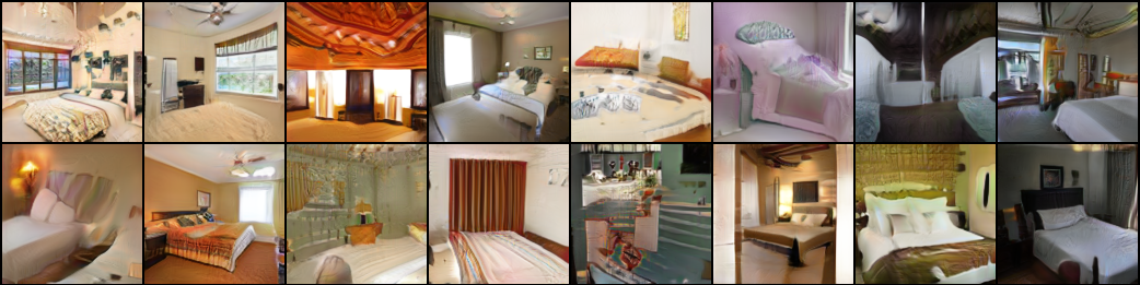
(a) WGAN-GP (FID: 13.6)

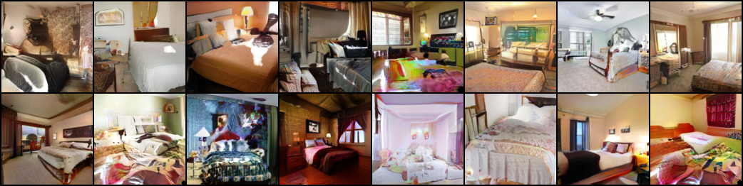
(b) SNGAN (FID: 13.2)

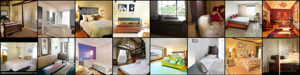
(c) GraND-GAN (FID: 10.8)

Figure 1: Images generated by WGAN-GP, SNGAN, and our method (GraND-GAN) on $128\times 128$ LSUN-Bedrooms (zoom in for better viewing). Lower FID is better.

Generative adversarial networks (GANs) [12] are a class of generative models that have been shown to be very effective, especially for unsupervised high-resolution image generation [30, 13, 18, 19]. GANs usually consist of two networks, a generator $G(z)$ that generates synthetic data conditioned on a noise vector $z$ (sampled from a known noise distribution, usually standard normal) and a discriminator (or critic) $D(x)$ that classifies real data from the generated synthetic data. $G$ and $D$ are generally parametrized as deep neural networks and optimize a mini-max objective. A Nash equilibrium of the zero-sum game is attained when $G$ models the real data distribution and $D$ is maximally uncertain in discriminating the real from synthetic samples.

Despite the effectiveness of GANs in modeling high-dimensional data distributions, they are hard to train. The quality of the images output by $G$ is dependent on the magnitude of the input gradients of the generator loss $\mathcal{L}_{G}$, written

$$\nabla_{x}\mathcal{L}_{G}(D(x))=\nabla_{D}\mathcal{L}_{G}(D(x))\nabla_{x}D(x),$$ (1)

where $x=G(z)$. The characteristics of the input gradient of $\mathcal{L}_{G}$, in general, are determined both by the architecture of the discriminator $D(x)$ as well as the loss function $\mathcal{L}_{G}$ used in formulating the mini-max objective. In turn, $\nabla_{x}D(x)$ is a function of the parameters $\theta_{D}$ of the discriminator (or critic) that is trained to minimize a loss $\mathcal{L}_{D}$ to separate real samples $x_{r}$ from the synthetically generated ones $x_{f}=G(z)$ for a given $G$. Therefore, in contrast to image classification, the role of $D$ is not only to accurately discriminate real data from fake or synthetic data, but also to have a well-behaved input gradient $\nabla_{x}D(x)$, which is the primary signal that $G$ relies on for learning. Designing such a discriminator is a major objective for GAN research.

Towards this goal, in this paper, we present a novel input-dependent normalization method called Gradient Normalization or GraN, which guarantees bounded gradients and a piecewise Lipschitz constraint almost everywhere. GraN can be applied to neural networks with piecewise linear activation functions, a prominent class of function approximators within deep learning, and we use the normalized output for discriminators (or critics). Fig. 1 shows a qualitative comparison of our method on the popular dataset LSUN-Bedrooms.

Other works have considered constraining $D$ for stabilizing GAN training. In contrast to spectral normalization [30], our method does not restrict processing at the individual layers and achieves a tight, piecewise Lipschitz bound on the class of functions that $D$ can model. Unlike gradient penalties [13], which softly penalize gradient norms at samples from the input space, our method strictly enforces piecewise constant gradients over the entire input space and ensures the gradient norms within each piece are strictly bounded by a single Lipschitz constant. However, our normalization introduces discontinuities in the discriminator itself, and it is only piecewise continuous and piecewise Lipschitz. Nevertheless, we show that our method achieves empirical results that are competitive with or better than existing methods.

Our main contributions are as follows:

• We present Gradient Normalization (GraN) for piecewise linear networks $f(x)$ that strictly constrains $f$ to be piecewise $\mathcal{K}$-Lipschitz, where the input space $x$ is partitioned into convex polytopes in each of which $f(x)$ is linear with $\|\nabla_{x}f(x)\|=\mathcal{K}$.

• We show that normalizing discriminators (or critics) with GraN bounds the gradients received by the generator $G$ almost everywhere, stabilizing GAN training.

• Unlike spectral normalization (SN), GraN does not restrict processing at the individual layers and does not suffer from gradient attenuation. Further, in contrast to both SN and gradient penalties, GraN enforces the piecewise Lipschitz property as a hard constraint.

• Empirically, GraN performs better or competitive to existing methods on multiple datasets (CIFAR-10, CIFAR-100, STL-10, LSUN bedrooms, and CelebA), and two loss functions (discriminators with a non-saturating cross-entropy loss and critics with a soft hinge loss).

• While GraN only enforces a local, piecewise Lipschitz constraint, we find the finite-difference gradient norm is empirically well-behaved across large step sizes, likely including jumps across the polytopes modeled by $f$.

• We also investigate the effect of the Lipschitz constant $\mathcal{K}$ on standard baseline models, finding (a) constrained discriminators (trained with cross-entropy loss) outperform constrained critics, (b) $\mathcal{K}$ influences training dynamics when using Adam, especially on loss plateaus, and (c) tuning $\mathcal{K}$ can significantly improve performance.

2 Related Work

2.1 Stabilizing GANs

Most previous works on stabilizing GANs take one of the following approaches: (1) proposing novel loss functions (e.g., [27, 4]), (2) devising improved architectures (e.g., [19, 43, 44, 31, 11, 9, 17]) or (3) introducing new constraints on $D$ (e.g., [2, 3, 34, 38]). Herein, we continue along the latter line of research, constructing an architectural regularization on $D$ that improves training without sacrificing network capacity.

One of the earliest works on constraining $D$ to stabilize GAN training is the Wasserstein GAN (WGAN) [3]. They propose a novel loss function and present weight-clipping as a way to regularize $D(x)$ to be 1-Lipschitz in $x$. However, subsequent work [13] showed gradient penalties to be more effective, as they do not impede optimization or severely reduce network capacity.

2.2 Gradient Penalties

Recent research has found gradient penalties (GPs), of the form $P_{\delta}(x)=(||\nabla_{x}f(x)||_{2}-\delta)^{2},$ to be useful for GANs. Building on WGAN, among the most popular GAN variants is WGAN-GP [13], which forgoes weight clipping by applying $P_{1}$ along random convex combinations of reals and fakes, since any $C^{0}$ function with unit-length gradient is necessarily 1-Lipschitz. Later research considered one-sided GPs [33], as well as alternate sampling methods [39].

Part of the motivation for turning to optimal transport distances is the reduction of gradient uninformativeness, which is a problem for most $f$-divergence-based GANs when the real and fake distributions do not sufficiently overlap [34]. However, Zhou et al. [45] show that Lipschitz continuity can combat gradient uninformativeness in GANs more generally. Separately, Roth et al. [34] showed that increasing distributional overlap via noise is approximately equivalent to a zero-centered GP. This was simplified to the popular “R1” GP (defined as $P_{0}$ on real data) [28], used in recent state-of-the-art GANs (e.g., [19, 7]).

Clearly, gradient regularization has seen empirical success in improving GANs. Yet, a downside of soft GPs is that they may not enforce exactly the desired value at a given position; furthermore, they are only applied to a subset of the input domain, which may shift over time. In contrast, GraN enforces unit gradients almost everywhere by construction.

2.3 Weight Normalization

Weight normalization (WN) [36] reparametrizes layers in a manner conducive to better conditioned optimization, used in early GAN work [35]. In WN, for each individual layer $i$ of the network, the corresponding weight vectors are rewritten as $\widetilde{w_{i}}=w_{i}{\rho_{i}}/{||w_{i}||}~{}\forall~{}i,$ where the learned scalar $\rho_{i}$ controls the norm and $w_{i}/{||w_{i}||}$ represents the direction.

For piecewise linear networks, each $x$ is linearly mapped to $f(x)=w\cdot x+b$, where $w$ is locally constant around $x$, is implicitly input-dependent, and may be interpreted as the effective weight vector of a (local) linear model (see §3.2 for details). In a manner reminiscent of WN, GraN essentially normalizes $f$ by the norm of its gradient, i.e., $\nabla_{x}f=||w||$. In contrast, however, GraN acts on the full network, rather than a single layer at a time, and enforces piecewise constant gradients, rather than reparametrizing the network.

2.4 Spectral Normalization and Gradient Attenuation under Global Lipschitz Constraints

Building on prior regularizations, such as GPs and weight clipping, Miyato et al. [30] present spectral normalization (SN) as an alternative method of ensuring $D$ is 1-Lipschitz, without an additional penalty in the objective for $D$. This is enforced by a layer-wise weight normalization technique, dividing by an estimate of the maximal singular value from each weight matrix. Empirically, SN is an effective stabilizer for GANs during training, independent of the loss function employed. As a result, it is a major component in recent large-scale GANs [6, 37]. We discuss SN further in §5.

At an architectural level, balancing network capacity and regularization is difficult for globally Lipschitz-constrained networks. Indeed, Anil et al. [1] showed that standard networks struggle to solve simple tasks when globally Lipschitz constrained, and that smooth SNed ReLU networks with unit gradients become globally linear, which they solve by enforcing gradient norm preservation and weight matrix orthonormality. We avoid this in GraN by permitting discontinuities in $D$ with respect to the input space and by only constraining the Lipschitz constant $\mathcal{K}$ locally in a piecewise manner. Later work [23] combated the gradient attenuation induced by Lipschitz constraints with a novel orthogonal convolution operator. In contrast, GraN can be applied on top of any piecewise linear network without globally constraining $\mathcal{K}$, while doing so locally in a piecewise sense.

3 Background

3.1 Generative adversarial networks

Let $\mathbb{P}_{r}$ represent the distribution of real data and $\mathbb{P}_{g}$ be the distribution of generated data at a given state of the generator $G$. Let $\mathcal{L}_{G}$ and $\mathcal{L}_{D}$ represent the loss functions for the generator $G$ and the discriminator (or critic) $D$, respectively. Let $z\sim\mathcal{N}(0,1)$ be a $|\mathcal{Z}|$-dimensional noise vector sampled from an i.i.d.  standard normal distribution. Let $f:\mathbb{R}^{d}\rightarrow\mathbb{R}$ represent a deep neural network encoding a scalar field. For image generation, $\mathbb{R}^{d}=\mathbb{R}^{3\times H\times W}$.

Goodfellow et al. [12] originally propose a cross-entropy (CE) loss-based objective for training $G$ and $D$ as follows:

$$\mathcal{L}_{D}=\mathbb{E}_{x\sim\mathbb{P}_{r}}\left[-\log D(x)\right]+\mathbb{E}_{x\sim\mathbb{P}_{g}}\left[-\log(1-D(x))\right],$$ (2)

$$\mathcal{L}_{G}=\mathbb{E}_{x\sim\mathbb{P}_{g}}\left[\log(1-D(x))\right],$$ (3)

where the discriminator $D(x)=\sigma(f(x))\in[0,1]$ represents the probability of a sample $x$ coming from the real distribution $\mathbb{P}_{r}$ and $\sigma(\cdot)$ is the sigmoid function $1/(1+e^{-(\cdot)})$. Hence, $f$ computes a logit mapped to a probability by $\sigma(\cdot)$. The gradient of $\mathcal{L}_{G}$ with respect to the inputs $x$ is then

$$\nabla_{x}\mathcal{L}_{G}=\mathbb{E}_{x\sim\mathbb{P}_{g}}\left[-D(x)\nabla_{x}f(x)\right].$$ (4)

Notice that, when $D(x)\rightarrow 0$ for some generated $x\sim\mathbb{P}_{g}$, the contribution to $\nabla_{x}\mathcal{L}_{G}$ from such points will necessarily be small and have little influence on updating $G$. This is particularly probable early in training, when $\mathbb{P}_{g}$ and $\mathbb{P}_{r}$ are easily separated. To overcome this problem, in the same work, the authors suggest using an alternative objective for $G$ that is non-saturating, given as

$$\mathcal{L}_{G}=\mathbb{E}_{x\sim\mathbb{P}_{g}}\left[-\log D(x)\right],$$ (5)

for which the gradient is

$$\nabla_{x}\mathcal{L}_{G}=\mathbb{E}_{x\sim\mathbb{P}_{g}}\left[-(1-D(x))\nabla_{x}f(x)\right].$$ (6)

In this case, note that when $D$ confidently rejects fakes (i.e., $D(G(z))\approx 0$), they can still contribute to $\nabla_{x}\mathcal{L}_{G}$. For future convenience of notation, we use “NSGAN” to refer to the non-saturating (NS) version of training a discriminator via a GAN, where $\mathcal{L}_{D}$ is given by Eq. (2) and $\mathcal{L}_{G}$ is given by Eq. (5). Note that although $\mathcal{L}_{G}$ in Eq. (5) is relatively non-saturating early in the training compared to Eq.  (3), it may still saturate later in training as $\mathbb{P}_{g}$ gets closer to $\mathbb{P}_{r}$.

Subsequently, the WGAN model [3] attempted to address two issues with the original GAN formulation. First, due to the use of the Jensen-Shannon divergence, disjoint support for $\mathbb{P}_{g}$ and $\mathbb{P}_{r}$ leads to poor gradients (as a confident $D$ rapidly saturates, leading to vanishing gradients). Second, for fixed $D$, the optimal $G$ samples a sum of Dirac deltas at points with the highest value of $D(x)$, leading to gradients that encourage mode collapse [29]. Using an approximate Wasserstein distance in WGANs mitigates these issues.

This WGAN objective for $G$ and critic $D$ may be written

$$\mathcal{L}_{D}=-\mathbb{E}_{x\sim\mathbb{P}_{r}}\left[D(x)\right]+\mathbb{E}_{x\sim\mathbb{P}_{g}}\left[D(x)\right],$$ (7)

$$\mathcal{L}_{G}=-\mathbb{E}_{x\sim\mathbb{P}_{g}}\left[D(x)\right],$$ (8)

where $D(x)=f(x)$, and $f(x)$ is constrained to be 1-Lipschitz in $x$, denoted by $\|f\|_{\text{Lip}}=1$. We now have

$$\nabla_{x}\mathcal{L}_{G}=\mathbb{E}_{x\sim\mathbb{P}_{g}}\left[-\nabla_{x}f(x)\right],$$ (9)

which does not saturate, unlike NSGAN (Eq. (6)).

Another commonly used variant of the critic loss $\mathcal{L}_{D}$ is the hinge loss [24, 30]:

$$\mathcal{L}_{D}=\mathbb{E}_{x\sim\mathbb{P}_{r}} \left[\text{ReLU}\left(1-D(x)\right)\right]+$$

$$\mathbb{E}_{x\sim\mathbb{P}_{g}}\left[\text{ReLU}\left(1+D(x)\right)\right],$$ (10)

where $\text{ReLU}(x)=\max\{0,x\}$ is the rectified linear unit. It is straightforward to define a smooth analogue of the hinge loss in Eq. (10) by using a smooth approximation of ReLU defined as $\text{SoftPlus}(x)=\log(1+e^{x})$, which we refer to as the soft hinge loss. For convenience of notation, we call $D$ a critic with $D(x)=f(x)$, when $\mathcal{L}_{D}$ is any of the Wasserstein, hinge, or soft hinge loss, and a discriminator with $D(x)=\sigma(f(x))$, when $\mathcal{L}_{D}$ is a variant of the cross-entropy loss (as in NSGANs).

For GANs, several methods have been proposed to effectively constrain $D$, generally to 1-Lipschitz function spaces. WGAN uses weight clipping, which compromises optimization ease and capacity, while WGAN-GP imposes a soft gradient penalty to improve upon this (see §2.1 and §2.2). More recently, SNGAN tries to impose a 1-Lipschitz constraint by enforcing unit spectral norm of every layer. In §5, we show that a composition of such constrained functions typically results in the overall Lipschitz constant being bounded loosely by 1, and discuss empirical results in §7.

While constraining $D$ to be 1-Lipschitz is necessary for training WGANs, Miyato et al. [30] empirically show that such a constraint is also beneficial when training NSGANs. One may immediately see why such smoothness constraints might help. Consider the norm of $\nabla_{x}\mathcal{L}_{G}$ for NSGANs (Eq. (6)) and WGANs (Eq. (9)) as follows

$$\|\nabla_{x}\mathcal{L}_{G}\|_{\text{NSGAN}} =\|\mathbb{E}_{x\sim\mathbb{P}_{g}}\left[-(1-D(x))\nabla_{x}f(x)\right]\|$$

$$\leq\mathbb{E}_{x\sim\mathbb{P}_{g}}\left[\|(1-D(x))\nabla_{x}f(x)\|\right]$$

$$\leq\mathbb{E}_{x\sim\mathbb{P}_{g}}\left[\|\nabla_{x}f(x)\|\right]$$ (11)

$$\|\nabla_{x}\mathcal{L}_{G}\|_{\text{WGAN}} =\|\mathbb{E}_{x\sim\mathbb{P}_{g}}\left[-\nabla_{x}f(x)\right]\|$$

$$\leq\mathbb{E}_{x\sim\mathbb{P}_{g}}\left[\|\nabla_{x}f(x)\|\right].$$ (12)

When $f$ is constrained to be $\mathcal{K}$-Lipschitz, clearly, $\|\nabla_{x}\mathcal{L}_{G}\|_{\text{NSGAN}}$ and $\|\nabla_{x}\mathcal{L}_{G}\|_{\text{WGAN}}$ are both bounded above by $\mathcal{K}$. This ensures that the gradients received by $G$ throughout the training are well-behaved and do not explode, thereby improving training stability.

In this paper, we introduce an alternative way to strictly bound the gradients by enforcing a piecewise $\mathcal{K}$-Lipschitz continuity almost everywhere (as opposed to a global $\mathcal{K}$-Lipschitz constraint). In a similar spirit to Miyato et al. [30], we empirically show that our method benefits both discriminators and critics.

In the next section, we introduce a notation for the class of functions implemented by deep neural networks with piecewise linear activations, and subsequently, in §4, we present gradient normalization for discriminators and critics.

3.2 Deep piecewise linear networks

Modern deep neural networks predominantly use piecewise linear activation functions such as ReLU and LeakyReLU. Such activation functions do not admit regions with saturation, and, hence, allow training very deep networks effectively without vanishing gradients.

Let $f(x):\mathbb{R}^{d}\rightarrow\mathbb{R}$ represent a (deterministic) deep neural network with piecewise linear activation functions. Denote the network parameters by $\theta$. Then one may write

$$f(x,\theta)=w(x,\theta)\cdot x+b(x,\theta),$$ (13)

where $w(x,\theta)$ and $b(x,\theta)$ are piecewise constant in $x$. We denote $w(x,\theta)\cdot x$ as the scalar dot-product of flattened tensors. Thus, $w(x,\theta)$ and $b(x,\theta)$ being piecewise constant in $x$ means that $\exists$ input sub-sets $S_{k}\in\left\{S_{j}\right\}_{j}\subseteq\mathbb{R}^{d}$, where

$$w(x\in S_{k},\theta) =w_{k}(\theta)\,~{}\text{and}~{}\,b(x\in S_{k},\theta)=b_{k}(\theta),$$

such that $w_{k}$ and $b_{k}$ are independent of $x$ within the sub-set $S_{k}$. Hence, $\forall x\in S_{k}$, we have

$$f(x\in S_{k},\theta)=w_{k}(\theta)\cdot x+b_{k}(\theta),$$ (14)

which is linear in $x\in S_{k}$. Then $f(x,\theta)$ is the composition of continuous, piecewise linear functions, and is therefore itself a continuous and piecewise linear function of $x$. That is, there exist disjoint open input subsets $S_{k}$, such that $\cup_{k=1}^{K}S_{k}=\mathbb{R}^{d}$, where Eq. 14 holds. I.e., $f(x,\theta)$ is a linear function of $x\in S_{k}$, with coefficients $w_{k}$ and $b_{k}$ that only depend on $\theta$. One can interpret $w_{k}(\theta)$ and $b_{k}(\theta)$ as the effective weights and bias of a linear functional (given by Eq.  (14)) that equals the predictions of the deep neural network, $f(x)$, $\forall~{}x\in S_{k}$. Note that, unlike a linear hyperplane in logistic regression, the effective weights $w_{k}(\theta)$ and bias $b_{k}(\theta)$ are only applicable for $x\in S_{k}$.

Given this structure, for points off of $\partial S_{k}$ (the boundary of $S_{k}$), the gradient takes a simple form:

$$\nabla_{x}f(x,\theta)=w_{k}(\theta),$$ (15)

which is a constant vector $\forall~{}x\in S_{k}$.

4 Gradient Normalization

In this section, we present gradient normalization (GraN), which strictly constrains piecewise linear networks to be 1-Lipschitz almost everywhere.

As in §3.2, let $f(x):\mathbb{R}^{d}\rightarrow\mathbb{R}$ represent a piecewise linear neural network with parameters $\theta$. We then define the gradient normalized function $g(x)$ as

$$g(x)=f(x)~{}\mathcal{R}_{\epsilon}(\|\nabla_{x}f(x)\|)=\frac{f(x)~{}\|\nabla_{x}f(x)\|}{\|\nabla_{x}f(x)\|^{2}+\epsilon},$$ (16)

where $\epsilon>0$ is a fixed constant for numerical stability and $\mathcal{R}_{\epsilon}(n)=n/(n^{2}+\epsilon)$ is the normalization factor, with $n=\|\nabla_{x}f(x)\|$. Any bounded $R(n)$, with $R(n)=(1/n)(1+o(1))$ as $n\rightarrow\infty$, could be tried. We briefly experimented with $R(n)=1/(n+\epsilon)$, which produced similar although slightly worse results than $\mathcal{R}_{\epsilon}$. The choice of $R(n)$ could benefit from further study. We remark that a concurrent work [41] to ours independently explores a similar technique to regularize $D$, but with a different normalization factor.

Given this normalization, if $f$ is an arbitrary piecewise linear function then $g$ is piecewise linear such that $\|\nabla_{x}g(x)\|\leq 1$ analytically almost everywhere in $x\in\mathbb{R}^{d}$. While the gradient $\nabla_{x}g(x)$ is bounded, $g(x)$ itself can still take real values with no bounds, i.e., $g(x)\in\mathbb{R}$.

One can better describe this result with the notation developed in §3.2. Consider an arbitrary input $x\in S_{k}$ (without any loss of generality) that belongs to the input open subset $S_{k}$ and is mapped by the network to a linear piece given by $f(x)=w_{k}(\theta)\cdot x+b_{k}(\theta)$ $\forall~{}x\in S_{k}$. Then one has $\nabla_{x}f(x,\theta)=w_{k}(\theta)$ $\forall~{}x\in S_{k}$ (Eq. (15)). Therefore, the GraNed function $g(x)$, given $f(x)$, for $x\in S_{k}$ becomes

$$g(x\in S_{k})=\left[w_{k}(\theta)\cdot x+b_{k}(\theta)\right]~{}\frac{\|w_{k}(\theta)\|}{\|w_{k}(\theta)\|^{2}+\epsilon}.$$ (17)

Consequently, $\nabla_{x}g$ and its norm can be written as

$$\nabla_{x}g(x\in S_{k})=w_{k}(\theta)~{}\frac{\|w_{k}(\theta)\|}{\|w_{k}(\theta)\|^{2}+\epsilon},$$ (18)

$$\implies\|\nabla_{x}g(x\in S_{k})\|=\frac{\|w_{k}(\theta)\|^{2}}{\|w_{k}(\theta)\|^{2}+\epsilon}<1.$$ (19)

Since $x$ and $S_{k}$ were arbitrarily chosen, it follows that $\|\nabla_{x}g(x)\|<1$ except at the boundaries, say $x\in\partial S_{k}$, where the gradient does not exist. Since $\cup_{k}\partial S_{k}$ is measure zero, we have $\|\nabla_{x}g(x)\|<1$ almost everywhere in $\mathbb{R}^{d}$. Further, for $\|w_{k}(\theta)\|\gg\epsilon$, we have $||\nabla_{x}g||\approx 1$ in $S_{k}$.

Note that, since the original piecewise linear function $f(x)$ does not have a smooth gradient $\nabla_{x}f(x)$, the normalization factor $\mathcal{R}_{\epsilon}(\|\nabla_{x}f(x)\|)$ will have discontinuities for $x\in\cup_{k}\partial S_{k}$. Therefore, $g$ is typically discontinuous and not guaranteed to be globally 1-Lipschitz. However, we empirically find that $g(x)$ has bounded finite-differences over substantial perturbations (see §7).

Due to this piecewise constant gradient property (with unit-bounded norm), we remark that $g$ is piecewise 1-Lipschitz, since $g$ is 1-Lipschitz with respect to any pair of points within each subset $S_{k}$. It is also locally 1-Lipschitz continuous almost everywhere, since there exists an open ball around every point $x\in\cup_{k}S_{k}$, within which 1-Lipschitz continuity holds. Empirically, we find that the tight bound on $\|\nabla_{x}g(x)\|$ almost everywhere assists with GAN training.

4.1 Gradient Normalized GANs

Given a deep neural network represented by $f(x)$, we write $D(x)=\sigma(f(x))$ when $D$ represents discriminators, and $D(x)=f(x)$, when $D$ represents critics, respectively, where $\sigma(\cdot)$ is the sigmoid function (see §3.1).

When $f(x)$ is piecewise linear in $x$, we define the gradient normalized discriminator (GraND) and critic (GraNC) as $D(x)=\sigma(g(x))$ and $D(x)=g(x)$, respectively, where

$$g(x)=\frac{f(x)}{\tau}~{}\frac{\|\nabla_{x}f(x)\|}{\|\nabla_{x}f(x)\|^{2}+\epsilon},$$ (20)

and $\tau$ is a positive constant that constrains $g$ to be $\mathcal{K}$-Lipschitz, with $\mathcal{K}=1/\tau$. For GraNDs, $\tau$ takes a role analogous to the temperature of a sigmoid, and, hence, we term it as the “temperature” hyperparameter.

Like spectral normalization [30], the Lipschitz constant $\mathcal{K}=1/\tau$ is the only additional hyperparameter that needs to be tuned for our method. Moreover, in practice, our method achieves a tight bound on the Lipschitz constant, unlike spectral normalization, which imposes a loose upper bound with $\|g\|_{\text{Lip}}\leq\mathcal{K}$. See §5 for details.

Finally, note that since the gradients in Eqs. (11) and (12) are computed by back-propagation, the step discontinuities in $g(x)$ are ignored. Therefore, for GANs with GraNDs and GraNCs, the generator $G$ receives gradients that are always bounded, i.e., $\|\nabla_{x}\mathcal{L}_{G}\|\leq\mathcal{K}$.

5 Comparison to Layer-wise Norms

Spectral Normalization As noted in §2.2, GPs softly encourage Lipschitz continuity in a data-dependent manner. Improving on this, the spectrally normalized GAN (SNGAN) [30] achieves it at the architectural level. In particular, a linear layer $\ell(x)=Wx$ (ignoring the bias term) with weights $W$ is normalized via $\widetilde{W}={W}/{||W||_{2}},$ before being applied to an input ($\widetilde{\ell}(x)=\widetilde{W}x$), where $||W||_{2}=\sigma_{1}(W)$ is the spectral norm of $W$, equal to its largest singular value (SV) $\sigma_{1}$. This is a form of WN, but acts on the whole matrix rather than its individual rows. Notice that $||\ell||_{\text{Lip}}\leq\sigma_{1}(W)$ and $\sigma_{1}(\widetilde{W})=1$, so $||\widetilde{\ell}||_{\text{Lip}}\leq 1$. As such, SN ensures layer-wise 1-Lipschitz continuity, and thus enforces it across the whole network, where SVs are estimated via power iteration.

One downside of SN is the tendency to over-constrain the network, reducing capacity and attenuating gradients, due to the layer-wise enforcement mechanism [1, 23]. SN guarantees a function is globally 1-Lipschitz by bounding the Lipschitz constant (LC) of every layer, as this then bounds their composition: $||f\circ g||_{\text{Lip}}\leq||f||_{\text{Lip}}||g||_{\text{Lip}}.$ However, this upper-bound is often loose, over-constraining the network and attenuating gradients (expanded upon below). In comparison, GraN acts upon the network as a whole, leaving weights per layer free to vary, and ensuring that gradients with respect to the input are always of unit norm.

The Looseness of Layerwise Constraints  For illustration, consider the simple case of two SNed linear layers without biases, ignoring non-linear activations (though, for instance, this occurs in the positive domain of ReLU): $z=f(g(x))$, where $f(y)=By$ and $g(x)=Ax$. Assuming sufficient power iterations under SN, the largest singular values (SVs) of $A$ and $B$ are one, assigning each layer an LC of one. We next examine the conditions for which the composition of the layers, $f\circ g$, also has a LC of one.

In this case, $z=f(g(x))=BAx$, and so $f\circ g$ has a sharp LC of one if and only if the maximal SV of $BA$, namely $\sigma_{1}(BA)$, is also one. Let $\Gamma_{\sigma}(A)$ denote the span of the right singular vectors of $A$ with corresponding SVs equal to $\sigma$. We show in appendix D, that $\sigma_{1}(BA)=1$ if and only if the first principal angle [10, 46] between the subspaces $\Gamma_{1}(A^{T})$ and $\Gamma_{1}(B)$ is zero. This only occurs if they intersect in at least one dimension. However, if even one SV of $A$ and $B$ is less than one, then $\Gamma_{1}(A^{T})$ and $\Gamma_{1}(B)$ will be measure zero, meaning the network must solve a high dimensional “alignment” problem of two measure zero sets. The only scenario avoiding this is when every SV of either $A$ or $B$ are one, which is also a measure zero event.

Importantly, since the SN framework does not directly encourage these subspaces to align, or all the SVs of the weight matrices to be one, in practice it is likely that $\sigma_{1}(BA)<1$. This issue is exacerbated for deeper networks, as the overall LC equals the product of $\sigma_{1}(BA)$ for every adjacent pair of layers. In addition, though training may encourage the network to utilize its capacity by avoiding small SVs, empirically it struggles to do so [1]. In contrast, GraN not only guarantees the function is locally 1-Lipschitz, but does so without constraining individual layers (avoiding subspace alignment issues) and enforces exactly unit gradient almost everywhere as well (attaining the sharp LC bound within every $S_{k}$). Fig. 3 displays this exactness for GraN; note that SNGAN, due its residual architecture, actually has an LC of 1024, showcasing the looseness of the bound.

Table 1: Hyperparameters tested in Fig. 2 for GraND-GAN, SNGAN, and WGAN-GP on CIFAR-10, where $\alpha$ is the learning rate, $\beta_{1}$ and $\beta_{2}$ parametrize Adam in Eq. (21), and $n_{\rm dis}$ is the number of discriminator steps per generator step.

Setting	$\alpha$ (LR)	$\beta_{1}$	$\beta_{2}$	$n_{\rm dis}$
A	0.0001	0.5	0.9	5
B	0.0002	0.5	0.999	1
C	0.001	0.5	0.999	5
D	0.001	0.9	0.999	5
E (default)	0.0002	0.0	0.9	5

(a) IS $\uparrow$

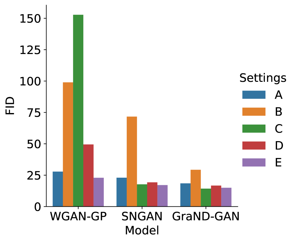
(b) FID $\downarrow$

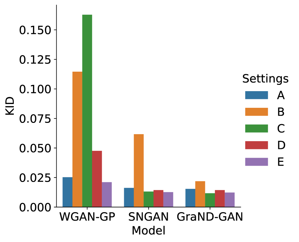
(c) KID $\downarrow$

Figure 2: Inception scores (IS), FIDs, and KIDs on CIFAR-10 image generation across different hyperparameters listed in Table 1 for GraND-GAN, WGAN-GP, and SNGAN. Results show superior robustness for GraND.

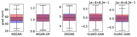
Figure 3: Boxplots of gradient norms at real (blue) and fake (red) samples for different methods at 50K iterations (out of 100K) on CIFAR-10 during training. Gradient norms for GraND/C have a very narrow distribution (spanning less than $\pm 10^{-6}$) around the piecewise Lipschitz constant $\mathcal{K}$=0.83.

6 Experiments

Model Architectures and Training We evaluate our method on unconditional image generation across datasets of various sizes: CIFAR-10/100 ($32\times 32$) [21], STL-10 ($48\times 48$) [8], LSUN bedrooms ($128\times 128$) [42], and CelebA ($128\times 128$) [26]. We use Mimicry [22] with PyTorch [32] on a single NVIDIA V100 GPU for training our models. The generator $G$ and discriminator (or critic) $D$ architectures are identical across methods for a given dataset with identical number of learnable parameters for fair comparison. We use the Adam [20] optimizer with $\beta_{1}=0.0$, $\beta_{2}=0.9$, and a batch size of $64$ for $100\text{K}$ iterations, with a dataset-dependent learning rate (LR) $\alpha$ and number of $D$ steps per $G$ step $n_{\rm dis}$. NSGANs and GraND-GAN use the cross-entropy loss for $D$ in Eq.  (2) and the non-saturating loss for $G$ in Eq. (5). GraNC-GAN uses a soft version of the hinge loss for $D$ in Eq. (10), replacing ReLU with softplus, and Eq. (8) for $G$ (see §3.1). The soft hinge loss was found to be more performant and stable than the (hard) hinge loss with GraNC-GANs: on LSUN, GraNC diverged with the hard hinge loss, while on CelebA, a lower FID was obtained. See appendix for further model details, ablation experiments, and hyperparameter choices.

Lipschitz Constant Analysis  We find that tuning the Lipschitz constant $\mathcal{K}$ significantly affects the performance and stability of models when using the Adam optimizer. This is due to the interdependence of $\epsilon_{\text{Adam}}$ in the update with $\mathcal{K}$:

$$\delta\mathbf{\theta}=-\frac{\langle\mathbf{g}\rangle_{\beta_{1}}}{\sqrt{\langle\mathbf{g}^{2}\rangle_{\beta_{2}}}+\epsilon_{\text{Adam}}}.$$ (21)

Changing $\mathcal{K}$ from its default value of one has an effect of scaling the gradients of the loss function $\mathbf{g}$ by $\mathcal{K}$. This in turn has an effect of scaling $\epsilon_{\text{Adam}}\longrightarrow\epsilon_{\text{Adam}}/\mathcal{K}$. Empirically, we find that the Adam update for individual parameters can go $\ll 10^{-7}$ in magnitude on the plateaus of the loss landscape where $\epsilon_{\text{Adam}}$ becomes significant. We find it helps having smaller $\mathcal{K}$ generally when training on larger image resolutions which has an effect of increasing $\epsilon_{\text{Adam}}$ from its default value of $1\times 10^{-8}$. Intuitively, a larger $\epsilon_{\text{Adam}}$ suppresses the Adam update when the loss gradient magnitudes are $\lesssim\epsilon_{\text{Adam}}$. Therefore, $\epsilon_{\text{Adam}}$ determines the extent of noisy Adam updates at plateaus of the loss landscape, and so may need tuning. More details on the choice of $\mathcal{K}$ are provided in the appendix.

Baselines and Evaluation  To directly compare our normalization method GraN with gradient penalty (GP) and spectral normalization (SN), independent of the loss function, we train NSGAN with a gradient penalty $P_{1}$ loss (NSGAN-GP), and with SNed layers (NSGAN-SN). We also train NSGAN-GP$\dagger$ and NSGAN-SN$\dagger$, which correspond to models constrained with a tuned Lipschitz constant (instead of 1). WGAN-GP$\dagger$ and SNGAN$\dagger$ are defined analogously.

We quantitatively evaluate the methods by Inception Score (IS) [35], FID [14], and KID [5] with 50K synthetic images randomly sampled from $G$ and 50K real images from the dataset. IS is not used for LSUN and CelebA, as these comprise a single class, for which IS performs poorly [22]. See appendix A for additional details.

Unconditional Image Generation  Table 2 presents the comparative results on CIFAR-10, CIFAR-100, and STL-10 image generation. Our methods rank among the top two across every metric (KID, FID, IS) on CIFAR-10 and CIFAR-100. On STL-10, our two methods rank the highest in IS and FID, however, we fall behind on KID by a small margin compared to SNGAN and SNGAN$\dagger$.

Table 3 summarizes our results on LSUN bedrooms and CelebA image generation. The NSGAN model did not converge (i.e., FID $>70$) in two random restarts of training for both LSUN and CelebA. Similarly, WGAN-GP failed to converge on CelebA in two runs. GraND-GAN achieves the best results on CelebA, and the second-best on LSUN bedrooms, falling slightly behind NSGAN-GP$\dagger$. Among critics, GraNC-GAN performs best by FID as well.

Table 2: Inception scores (IS), FIDs, and KIDs with unsupervised image generation on CIFAR-10, CIFAR-100, and STL-10. The best and the second best models per evaluation metric and GAN family (i.e., with discriminators or critics) are indicated by bold red and bold blue fonts. $\dagger$ indicates modified baselines with an altered Lipschitz constant $\mathcal{K}$. The table is split comparing discriminators (top) and critics (bottom). We write “–” for cases where a model did not achieve a FID $<70$.

Method	IS $\uparrow$			FID $\downarrow$			KID (${\times}1000$)  $\downarrow$
	CIFAR-10	CIFAR-100	STL-10	CIFAR-10	CIFAR-100	STL-10	CIFAR-10	CIFAR-100	STL-10
NSGAN	7.655	6.611	7.920	23.750	30.842	44.179	14.5	20.5	40.0
NSGAN-GP	8.016	–	8.568	15.813	–	38.848	12.9	–	38.9
NSGAN-SN	7.792	7.258	8.167	20.998	25.564	38.669	15.7	18.4	35.7
NSGAN-GP$\dagger$	8.019	7.892	8.623	15.911	20.894	40.110	13.1	17.0	39.8
NSGAN-SN$\dagger$	7.814	7.526	8.135	20.323	24.200	39.013	15.3	17.7	36.7
GraND-GAN (Ours)	8.031	8.314	8.743	14.965	18.978	35.226	12.3	13.7	35.0
WGAN-GP	7.442	7.520	8.492	22.927	27.231	42.170	21.1	23.5	43.0
SNGAN	8.112	7.778	8.385	17.107	20.739	38.218	12.6	14.3	34.3
WGAN-GP$\dagger$	7.344	7.684	8.466	22.705	25.211	42.595	20.6	21.2	44.7
SNGAN$\dagger$	7.991	7.959	8.552	16.740	20.104	36.203	12.0	14.3	33.3
GraNC-GAN (Ours)	7.966	8.208	8.957	16.361	19.131	35.770	13.7	14.8	35.4

Table 3: Unsupervised $128\times 128$ image generation on LSUN-Bedrooms and CelebA. We write “–” to indicate the cases where a model did not achieve a FID $<70$ in two random training restarts. The best and the second best models per evaluation metric and GAN family (i.e., with discriminators or critics) are indicated by bold red and bold blue fonts. $\dagger$ indicates modified baselines with an altered Lipschitz constant $\mathcal{K}$. We split the table into discriminators (top) and critics (bottom), to better highlight the differences per loss function. GraN performs best or second-best across all datasets, losses, and performance metrics; in the case of discriminators, GraND-GAN and NSGAN-GP$\dagger$ (our Lipschitz-tuned GP-based approach) are the top two performers.

Method	FID $\downarrow$		KID (${\times}1000)$ $\downarrow$
	LSUN	CelebA	LSUN	CelebA
NSGAN	–	–	–	–
NSGAN-GP	–	–	–	–
NSGAN-SN	74.926	14.33	44.8	21.2
NSGAN-GP$\dagger$	10.483	9.385	7.2	5.8
NSGAN-SN$\dagger$	12.635	9.644	8.3	5.8
GraND-GAN (Ours)	10.795	9.377	7.3	5.2
WGAN-GP	13.562	–	9.8	–
SNGAN	13.237	13.466	8.0	8.9
WGAN-GP$\dagger$	16.884	–	12.0	–
SNGAN$\dagger$	67.346	15.874	32.0	8.7
GraNC-GAN (Ours)	12.533	12.000	9.1	8.1

Figure 2 presents a comparison of GraND-GAN with WGAN-GP and SNGAN on CIFAR-10 image generation across various training settings listed in Table 1. For setting B ($n_{\rm dis}$ = 1), our method retains a respectable FID score (and other metrics) compared to SNGAN and WGAN-GP. For settings C and D with larger learning rates and momentum hyperparameters, the performance of WGAN-GP degrades while our method and SNGAN remain quite robust.

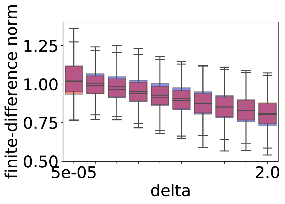
(a) WGAN-GP

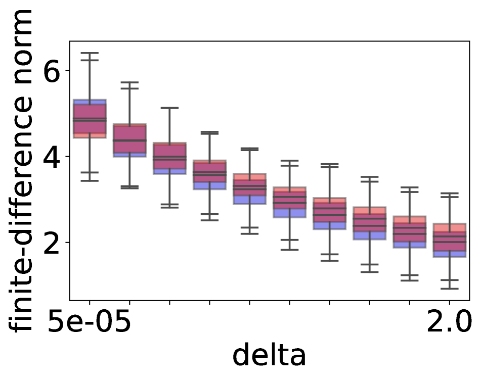
(b) SNGAN

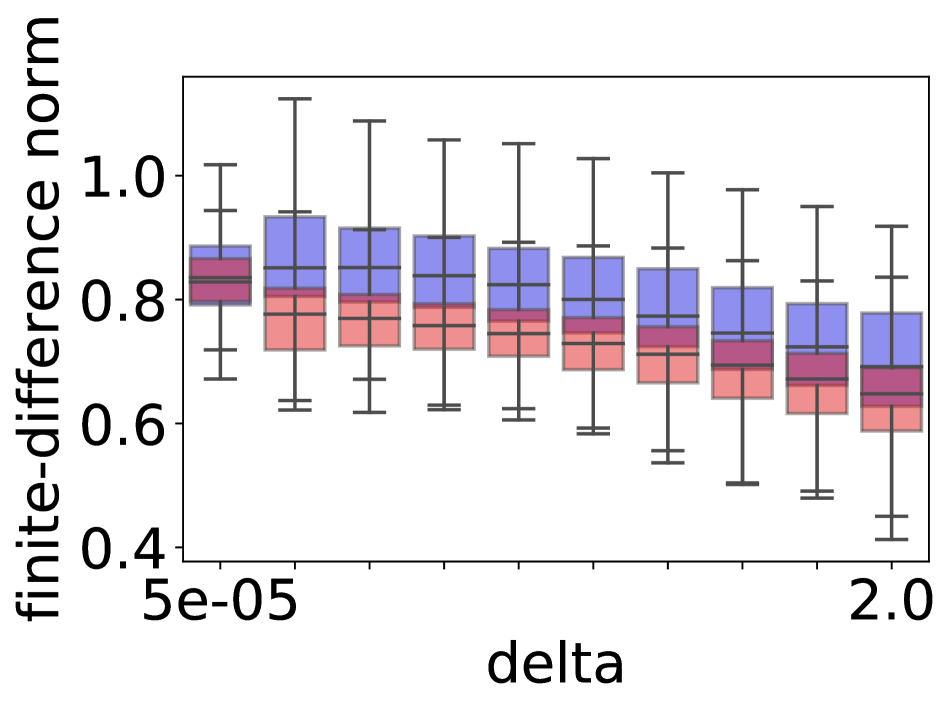
(c) GraND-GAN

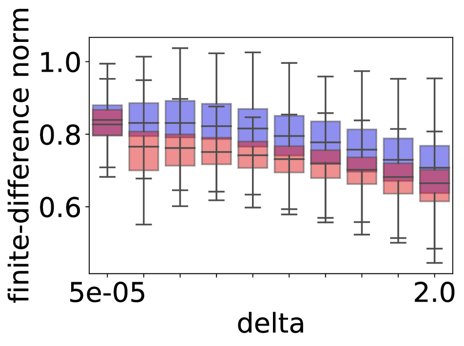
(d) GraNC-GAN

Figure 4: Boxplots of estimated finite-difference gradient norm with increasing $L2$ perturbation strengths $\delta$ around the real (blue) and fake samples (red) on CIFAR-10 at 50K iterations (out of 100K) for different methods. Empirically, GraND/C is fairly Lipschitz bounded across polytopes globally, close to the piecewise Lipschitz constant of $\mathcal{K}=0.83$.

7 Gradient Normalization Empirical Analysis

In this section, we empirically analyze the effect of gradient normalization on (a) the gradient norms and (b) the finite-difference approximation to the gradient norm at increasing levels of perturbation $\delta$, and compare it with spectral normalization and gradient penalty.

Figure 3 shows a boxplot of $\|\nabla_{x}f(x)\|$ for the baselines, and $\|\nabla_{x}g(x)\|$ for our methods, on a CIFAR-10 image generation task at 50K iterations (out of 100K), where $f(x)$ is the piecewise linear discriminator (or critic) network and $g(x)$ is its gradient normalized version. The gradient norms $\|\nabla_{x}f(x)\|$ for NSGAN with an unconstrained discriminator are substantially larger. For WGAN-GP and SNGAN, $\|\nabla_{x}f(x)\|$ are bounded within a reasonable range. Gradient normalized discriminators and critics with a piecewise Lipschitz constant of $\mathcal{K}=0.83$, have a narrow distribution with a gradient norm that is $\approx\mathcal{K}$ ($\pm 10^{-6}$) across samples.

Unlike spectral normalization or gradient penalty, our method does not constrain the discriminator or critic to be globally $\mathcal{K}$-Lipschitz. We investigate this on a CIFAR-10 image generation task by first sampling fake data from $G$ at a given training iteration and real data from the dataset. We estimate $\Delta_{i}=\|h(x_{i}+\delta n_{i})-h(x_{i})\|/\delta$ for each of the samples, which is the finite difference along a step of magnitude $\delta>0$ along the local gradient direction $n_{i}=\nabla h(x_{i})/\|\nabla h(x_{i})\|$, where $h$ denotes $f$ for baselines and $g$ for our methods, respectively. This provides a probe for the LC (albeit a lower bound) similar in spirit to prior work [47].

Figure 4 shows a boxplot of the resulting $\Delta_{i}$ for increasing perturbation magnitudes $\delta$. Evidently, gradient normalized discriminators and critics have well-behaved finite-differences, even for fairly large neighborhoods $\delta$, despite being only piecewise Lipschitz in theory. Moreover, the variance of the computed $\Delta_{i}$’s across $\delta$ for our methods is comparable to WGAN-GP.

8 Discussion

Limitations  We observed instabilities when training gradient normalized critics with the Wasserstein loss (Eq. (7)). The hinge loss (Eq. (10)) improved this, but still struggled for larger images; the soft hinge approach was found to work better. However, training GraND with the NS loss (Eq. (2)) was found to be more stable, especially on larger images. Also, on such images, our method periodically diverged late in training, an issue present for the baselines as well.

Future work  While GraN does not guarantee a global Lipschitz constraint due to discontinuities, it does enforce constant bounded-norm gradients almost everywhere (and thus piecewise Lipschitz continuity). Moreover, empirically, it is competitive with, or better than, existing baselines. Investigating global versus local Lipschitz continuity, as well as gradient regularization, is thus an enticing future direction.

Conclusion  We introduced a novel input-dependent normalization for piecewise linear critics and discriminators. Our method guarantees a bounded input gradient norm almost everywhere and is piecewise $\mathcal{K}$-Lipschitz. We empirically showed that our method improves unconditional image generation using GANs across a range of datasets. Finally, though our method does not explicitly impose a global $\mathcal{K}$-Lipschitz constraint, empirically, the finite-difference gradient norm is well-behaved in a large local neighbourhood.

Appendix

Appendix A Training Details

We use Mimicry [22] with PyTorch [32] on a single NVIDIA V100 GPU for training our models. The generator $G$ and discriminator (or critic) $D$ architectures are identical across methods for a given dataset except for models with spectral normalization that replace convolutional and linear layers with their normalized variants. The number of learnable parameters are identical across methods for a fixed dataset size. Number of parameters for $(G,D)$ are $\approx$ $(4.3\text{M},1\text{M})$ for $32^{2}$, $(4.9\text{M},10\text{M})$ for $48^{2}$, and $(32\text{M},29\text{M})$ for $128^{2}$ image sizes, respectively. $G$ and $D$ are both residual networks with ReLU activation functions, and $G$ employs batch normalization [15] while $D$ does not. We train our models on a single NVIDIA V100 GPU with the Adam [20] optimizer at a learning rate (LR) of $2\times 10^{-4}$, $\beta_{1}=0.0$, $\beta_{2}=0.9$ and a batch size of $64$ for $100\text{K}$ iterations. The number of discriminator updates per generator update $n_{dis}$ is set to $5$ for CIFAR-10/CIFAR-100/STL-10 and $2$ for LSUN bedrooms/CelebA. All models (GraN or baseline) use a linear LR decay policy except models on CelebA that use the same learning rate throughout, following Mimicry [22]. However, GraNC-GAN on CelebA required a slight alteration: setting LRs for $G$ and $D$ to be $5\times 10^{-5}$ and $1\times 10^{-4}$, respectively, and using linear LR decay.

Empirically we find it necessary to have a smaller piecewise Lipschitz constant $\mathcal{K}$ when training GANs on larger image resolutions with gradient normalization. We suspect that a smooth discriminator or critic with smaller gradient norms is essential for stable GAN training on larger image resolutions. We choose $\mathcal{K}=1/\tau=0.0909$ for our models on LSUN bedrooms/CelebA (except for $\mathcal{K}=1/\tau=0.2$ with GraNC-GAN on CelebA) and $\mathcal{K}=1/\tau=0.83$ for our models on CIFAR-10/CIFAR-100/STL-10.

WGAN-GP uses the Wasserstein distance based loss objectives for $D$ in Eq. (7) and $G$ in Eq. (8). SNGAN uses hinge loss for $D$ in Eq. (10) and Eq. (8) for $G$.

For NSGAN-GP$\dagger$, we adjust the gradient penalty loss to constrain the Lipschitz constant to $\mathcal{K}$ (instead of 1). For NSGAN-SN$\dagger$, we scale the output of the network before the sigmoid by $\mathcal{K}$ to obtain an effective $\mathcal{K}$-Lipschitz constraint using SN. We also retrain the baselines WGAN-GP and SNGAN with similar modifications so that the Lipschitz constraint is identical to the piecewise Lipschitz constraint for our methods and call them WGAN-GP$\dagger$ and SNGAN$\dagger$, respectively.

It is also worth highlighting that our method backpropagates through the GraN normalization term as well and does not simply treat it as a constant.

Evaluation

We quantitatively evaluate the methods by Inception Score (IS) [35], FID [14], and KID [5] with 50K synthetic images randomly sampled from $G$ and 50K real images from the dataset. We report the mean scores computed across 3 randomly sampled sets of 50K images for a given $G$. We note that across all methods and datasets, the standard deviations across 3 evaluation samplings for IS, FID, and KID are less than 0.05, 0.085, and 0.0004, respectively, and we therefore do not include them in our tables. IS is not used for LSUN and CelebA, as these comprise a single class, for which IS performs poorly [22].

Appendix B Model Architectures

Figure 5 presents the discriminator model architectures for inputs of dimensions $32^{2}$, $48^{2}$ and $128^{2}$, respectively. Figure 6 presents the generator model architectures for outputs of dimensions $32^{2}$, $48^{2}$ and $128^{2}$, respectively.

Note that for GraN-models, the output of the networks $f(x)$ is normalized to $g(x)$ as described in Equation (19) of the main paper and does not contain any additional learnable parameters.

To modify the Lipschitz constant (LC) of baselines involving spectral normalized linear and convolutional layers (NSGAN-SN$\dagger$ and SNGAN$\dagger$), we scale the output $f(x)$ by $\mathcal{K}$, i.e., $f(x)\rightarrow\mathcal{K}f(x)$, where $\mathcal{K}$ scales LC relative to the LC of the baseline model since $|f|_{\text{Lip}}\leq 1$, implies, $|\mathcal{K}f|_{\text{Lip}}\leq\mathcal{K}$.

For models WGAN-GP$\dagger$ and NSGAN-GP$\dagger$, we instead only change the gradient penalty loss term in the objective for $D$ to

$$\mathcal{L}_{\text{GP}}=\lambda\left(\|\nabla_{x}f(x)\|-\mathcal{K}\right)^{2},$$

where $\lambda=10$ (following defaults recommended in [13]) and $\mathcal{K}=1$ corresponds to the default WGAN-GP model. As in the main paper, we denote $\dagger$ to represent models with adjusted LC relative to the original baselines.

See also §D and Fig. 8 for discussion and empirical results concerning the observed LC when using an SNGAN discriminator with a resnet-based convolutional architecture.

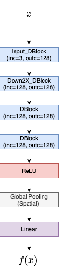
(a) $x\in\mathbb{R}^{32^{2}}$

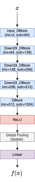
(b) $x\in\mathbb{R}^{48^{2}}$

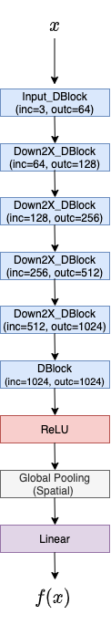
(c) $x\in\mathbb{R}^{128^{2}}$

Figure 5: Discriminator architectures for a) $32\times 32$, b) $48\times 48$ and c) $128\times 128$ image sizes, respectively. The architectures for Input_DBlock, DBlock and Down2X_DBlock are described in Figure 7. All models use Global Spatial Average Pooling except SNGAN that uses Global Spatial Sum Pooling before the last Linear layer. For SNGAN only, the Linear and convolution Conv2D layers are the spectral normalized versions with 1 power iteration.

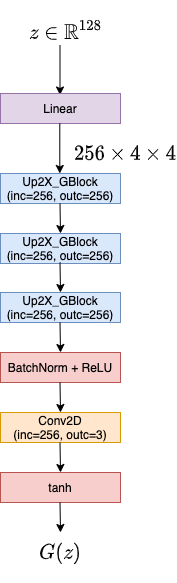
(a) $G(z)\in\mathbb{R}^{32^{2}}$

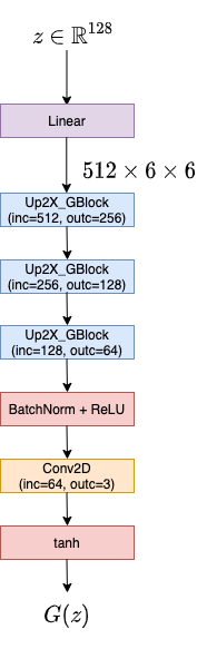
(b) $G(z)\in\mathbb{R}^{48^{2}}$

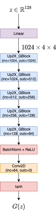
(c) $G(z)\in\mathbb{R}^{128^{2}}$

Figure 6: Generator architectures for a) $32\times 32$, b) $48\times 48$ and c) $128\times 128$ image sizes, respectively. The architecture for Up2X_GBlock is described in Figure 7. Generator architectures are identical across all models for a given dataset resolution.

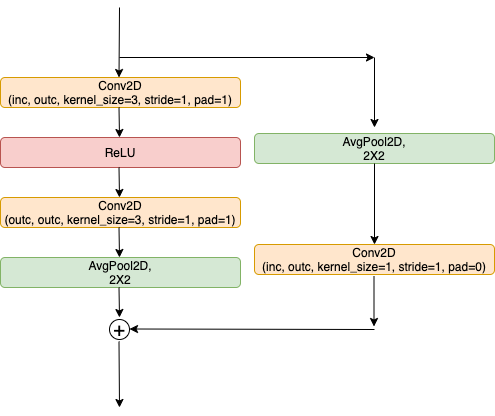
(a) Input_DBlock

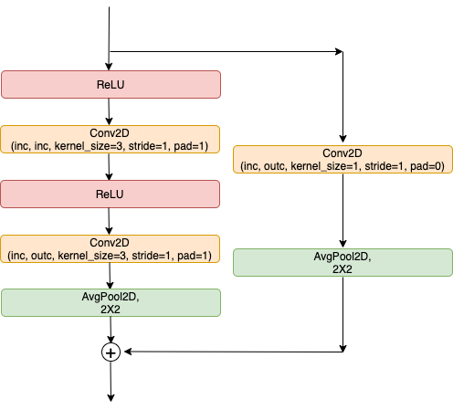
(b) Down2X_DBlock

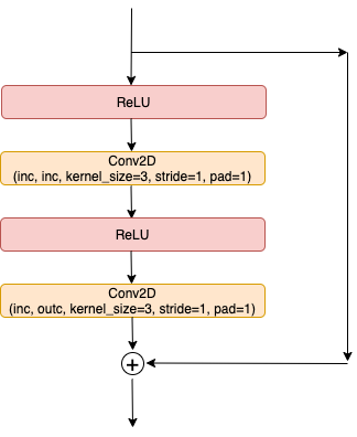
(c) DBlock

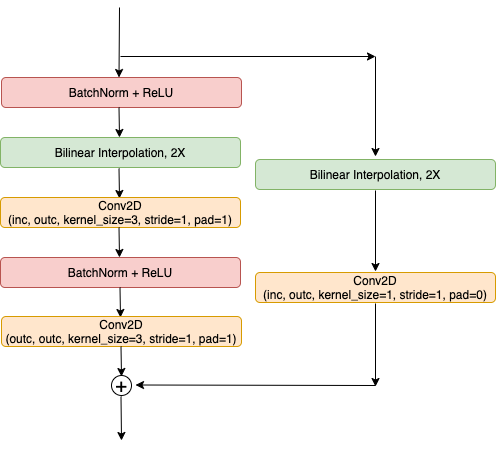
(d) Up2X_GBlock

Figure 7: Residual block architectures for a) Input_DBlock, b) Down2X_DBlock, c) DBlock and d) Up2X_GBlock in Figures 5 and 6. inc and outc denote the input and output number of channels, respectively. Note that when $\texttt{inc}\neq\texttt{outc}$, the skip connection in DBlock includes a $1\times 1~{}\texttt{Conv2D}$ appropriately. For SNGAN, the linear and convolution layers in Input_DBlock, DBlock and Down2X_DBlock are the spectral normalized versions.

Appendix C Wall-clock timings for a single training update

We summarize wall-clock times for a single training update that consists of one generator update and $n_{dis}$ number of discriminator updates (including time for loading a batch of $64$ images from the dataset). As can be noticed from Table 4, our method is roughly similar in wall-clock timings compared to WGAN-GP on smaller models ($32^{2}$ and $48^{2}$) but slower than NSGAN or SNGAN. On $128^{2}$ images GraN is 40% slower than WGAN-GP.

Table 4: Wall-clock timings (in seconds $\times 10$) for a single training update across different dataset of different resolutions. Note that $n_{dis}=5$ for CIFAR-10/100 and STL-10 while $n_{dis}=2$ for LSUN/CelebA, following Mimicry [22].

Method	CIFAR-10	CIFAR-100	STL-10	LSUN	CelebA
	sec ($\times 10$)	sec ($\times 10$)	sec ($\times 10$)	sec ($\times 10$)	sec ($\times 10$)
NSGAN	3.80$\pm$0.04	3.72$\pm$0.03	4.89$\pm$0.06	10.93$\pm$0.10	10.98$\pm$0.10
WGAN-GP	5.86$\pm$0.46	6.12$\pm$0.13	8.19$\pm$0.18	18.78$\pm$0.10	18.61$\pm$0.10
SNGAN	4.17$\pm$0.05	4.17$\pm$0.04	5.57$\pm$0.11	11.62$\pm$0.11	11.56$\pm$0.09
GraND-GAN (Ours)	5.66$\pm$0.04	5.69$\pm$0.04	8.83$\pm$0.07	26.34$\pm$0.08	26.13$\pm$0.10
GraNC-GAN (Ours)	5.69$\pm$0.04	5.65$\pm$0.04	8.83$\pm$0.08	26.11$\pm$0.10	26.18$\pm$0.18

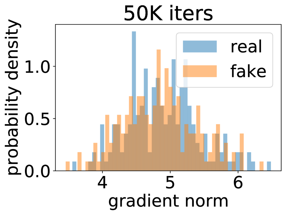
(a) Gradient norm (SNGAN with sum pooling)

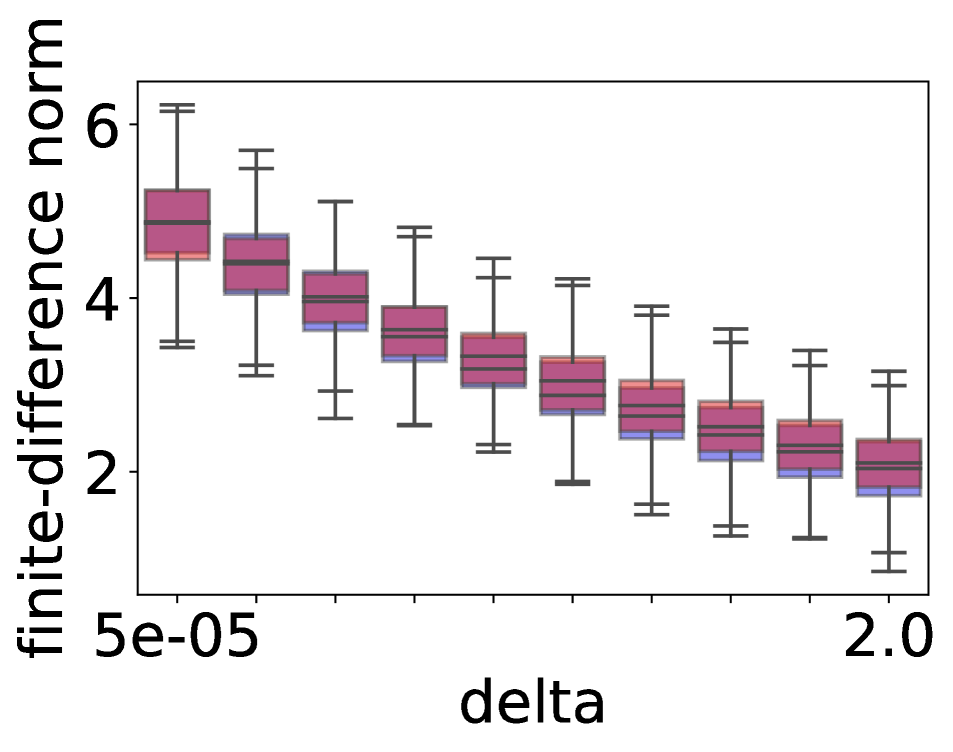
(b) FD gradient norm (SNGAN with sum pooling)

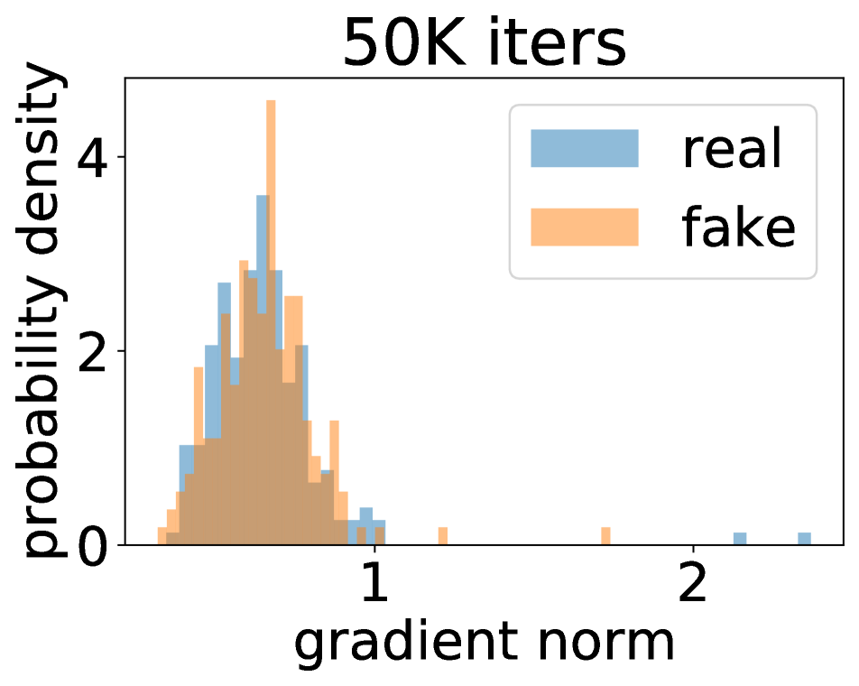
(c) Gradient norm (SNGAN with average pooling)

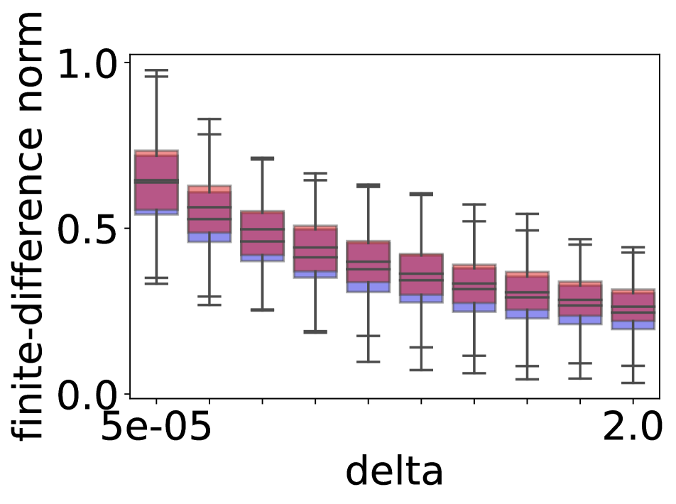
(d) FD gradient norm (SNGAN with average pooling)

Figure 8: Gradient norms and finite-difference (FD) approximation to the gradient norms at increasing perturbation length delta along the gradient for SNGAN with global sum pooling ((a) and (b)) and global average pooling ((c) and (d)) at 50K iterations of training on CIFAR-10.

This is because gradient normalized discriminator (or critic) $D$ requires computing the gradient norms on both the real and the fake samples when updating the parameters of $D$. In contrast, WGAN-GP only computes gradient norms on half the total number of real$+$fake samples which are random interpolates between the reals and fakes. Moreover, when updating $G$, computing generator loss $\mathcal{L}_{G}$ requires computing the gradient norm of $D$ for GraN models, unlike WGAN-GP where gradient penalty affects only the parameter updates for $D$ at a given training iteration. GraN and WGAN-GP are both slower relative to NSGAN or SNGAN because they involve computing the gradient norm and backpropagating through it. We remark that further advances in the efficiency of back-propagation through network gradients could ameliorate this issue (e.g., AutoInt [25]).

However, we note that, since the generator $G$ architecture is identical across methods for a given dataset, at inference all methods fare equally in wall-clock timings for image generation.

Appendix D The Looseness of Layerwise Constraints

We consider the simple case of the composition of two linear layers, $z=f(g(x))=B(Ax+a)+b$, where both $f$ and $g$, have a sharp Lipschitz constant (LC) of one. The question is under what conditions does $f\circ g$ also have a sharp LC of one?

We first introduce some notation. Let $M$ be an $m\times n$ matrix. We denote the singular value decomposition of $M$ as $M=U_{M}\Sigma_{M}V_{M}^{T}$, where we take $U_{M}$ and $V_{M}$ to be square matrices (of sizes $m\times m$ and $n\times n$, respectively). Here $\Sigma_{M}$ is a diagonal $m\times n$ matrix, with the non-negative singular values sorted in decreasing order down the diagonal [10]. Define $\sigma_{1}(M)$ to be the maximal SV of the matrix $M$. Moreover, define $\Gamma_{\sigma}(M)$ to be the projection from $\mathbb{R}^{n}$ to the subspace spanned by the right singular vectors of $M$ for SV’s equal to $\sigma$. That is,

$$\Gamma_{\sigma}(M)=V_{M}D_{\sigma}(M)V_{M}^{T},$$ (22)

where $D_{\sigma}(M)$ is defined to be a diagonal $n\times n$ matrix where the $i^{th}$ diagonal element is $1$ when the corresponding element of $\Sigma_{M}$ equals $\sigma$, and zero otherwise. It then follows that $\Gamma_{\sigma}(M^{T})$ is the projection of $\mathbb{R}^{m}$ to the subspace spanned by the left singular vectors of $M$ for the SV $\sigma$. Finally, from the form of $\Gamma_{\sigma}(M)$ in (22) we can conclude

$$\sigma_{1}(\Gamma_{\sigma}(M))=1,$$ (23)

$$\Gamma_{\sigma}(M)\Gamma_{\sigma}(M)=\Gamma_{\sigma}(M),$$ (24)

so long as $\sigma$ is an SV for $M$.

We can express the conditions that $f$, $g$, and $f\circ g$ all have sharp LC of one in terms of this notation. Specifically, the tight Lipschitz bounds for $f$, $g$ and $f\circ g$ are $\sigma_{1}(B)$, $\sigma_{1}(A)$, and $\sigma_{1}(BA)$, respectively. Assuming SN has rescaled $A$ and $B$ appropriately, then the LC of $g$ and $f$ are both one and we have $\sigma_{1}(B)$ $=$ $\sigma_{1}(A)$ $=$ $1$. Moreover, we see $f\circ g$ will have a sharp LC of one iff $\sigma_{1}(BA)$ $=$ $1$. We examine this latter condition.

Theorem 1.

For $A$ and $B$ as above (with dimensions such that their product $BA$ can be formed), with maximal SV’s equal to one, the maximal SV of $BA$ satisfies $\sigma_{1}(BA)\leq 1$. Further, equality of this bound holds if and only if

$$\sigma_{1}(\Gamma_{1}(B)\Gamma_{1}(A^{T}))=1.$$ (25)

Proof of Theorem 1. Let $m_{1}=\text{dim}(\Gamma_{1}(A))$ and $n_{1}=\text{dim}(\Gamma_{1}(B))$ be the number of singular values equal to one in $A$ and $B$, respectively. The assumption that $\sigma_{1}(A)=\sigma_{1}(B)=1$ implies $m_{1},n_{1}>0$.

Recall that the spectral norm of a matrix $M$, which is induced by the $L_{2}$ vector norm, can be defined via the largest singular value: $||M||_{2}:=\sigma_{1}(M)$, equivalently computed as

$$||M||_{2}=\sup_{||x||=||y||=1}|y^{T}Mx|=\sup_{x\neq 0}\frac{||Mx||}{||x||}.$$ (26)

It follows from (26) that $||BA||_{2}\leq||B||_{2}||A||_{2}$ (the submultiplicativity property), and hence

$$\sigma_{1}(BA)\leq\sigma_{1}(B)\sigma_{1}(A)=1.$$ (27)

First we prove $\sigma_{1}(BA)=1$ implies (25). Assume $\sigma_{1}(BA)=1$. Then it follows from (26) that there exists a vector $x$ such that $||x||=1$ and $z:=BAx$ satisfies $||z||=1$. Let $y=Ax$. There are two cases to consider, either $||y||<1$, or $||y||=1$. However, since $z=By$ and $||B||_{2}=\sigma_{1}(B)=1$ we have $||z||<=||B||_{2}||y||=||y||$. Therefore the assumption $||y||<1$ leads to the contradiction $||z||<1$, and instead we must have

$$||y|| =||Ax||=||x||=1,$$ (28)

$$||z|| =||By||=||y||=1.$$ (29)

Equation (28) ensures $x\in\mbox{\tt range}(\Gamma_{1}(A))$ and therefore $y=Ax\in\mbox{\tt range}(\Gamma_{1}(A^{T}))$. Also, equation (29) ensures $y\in\mbox{\tt range}(\Gamma_{1}(B))$. Therefore it follows that $y$ is a unit vector such that $\Gamma_{1}(B)y=y$, and $\Gamma_{1}(A^{T})y=y$. And thus, $\Gamma_{1}(B)\Gamma_{1}(A^{T})y=y$. By (26) we then have $\sigma_{1}(\Gamma_{1}(B)\Gamma_{1}(A^{T}))\geq 1$. But, from (23), it follows that $\sigma_{1}(\Gamma_{1}(B))=\sigma_{1}(\Gamma_{1}(A^{T}))=1$ and therefore $\sigma_{1}(\Gamma_{1}(B)\Gamma_{1}(A^{T}))\leq 1$. As a result we have shown (25), as desired.

For the reverse direction, assume $\sigma_{1}(\Gamma_{1}(B)\Gamma_{1}(A^{T}))=1$. Then (26) implies there exists a $y$ such that $||y||=1$ and $z=\Gamma_{1}(B)\Gamma_{1}(A^{T})y$ with $||z||=1$. But, since $\Gamma_{1}(B)$ and $\Gamma_{1}(A^{T})$ are projection matrices (see (24)), it can be shown that we must have $\Gamma_{1}(A^{T})y=y$, $\Gamma_{1}(B)y=y$, and $z=y$. Moreover, since $y$ is a right singular vector of $A^{T}$ for singular value one, it follows that $x:=A^{T}y=V_{A}\Sigma_{A}U_{A}^{T}y$ is a left singular vector of $A^{T}$ for the SV at one and $||x||=1$. Therefore $x=\Gamma_{1}(A)x=V_{A}D_{1}(A)V_{A}^{T}x$. That is, $x$ is in the right singular space of $A$ for the SV at one and it follows that $y=Ax$. Taken together, we have $BAx$ $=$ $By$ and $y=\Gamma_{1}(B)y$, so $||By||=1$. Hence $||BAx||=||By||=1=||x||$ . That is, from (26), it follows that $\sigma_{1}(BA)\geq 1$. Finally, from (27), we conclude $\sigma_{1}(BA)=1$, as desired. $\square$

Relation to Layerwise Spectral Normalization  As described in the text, (Eq. 25) is a subspace alignment condition where $\sigma_{1}(\Gamma_{1}(B)\Gamma_{1}(A^{T}))$ equals the cosine of the first principal angle between the two subspaces $\Gamma_{1}(B)$ and $\Gamma_{1}(A^{T})$ [10, 46]. It is therefore unlikely to be satisfied by chance, although during training the model may reduce this angle and approach $\sigma_{1}(\Gamma_{1}(B)\Gamma_{1}(A^{T}))=1$. Thus, with training, we might expect the norm of the gradients of $f(x)$ to increase towards an upper bound.

However, we note additional features of $f(x)$ for the architectures described in Figures 5 and 7. Specifically, the global sum pooling in Fig. 5 and the skip connections in Fig. 7 are both capable of amplifying the gradient norms through these stages by a factor greater than one. Thus, while the subspace alignment conditions can be expected to shrink the gradient magnitudes, these specific components can expand them. The consequence of these two opposing effects is not clear a priori.

The empirical results shown in Fig. 8(a) indicate that, for the cases tested, the net effect is for $f(x)$ to have a gradient norm larger than one. Moreover, when average pooling is used in place of the sum pooling, the norm of the gradient is predominantly less than one (see Fig. 8(c)). Similar properties are seen for the magnitudes of finite differences (FD) of $f(x)$ over steps of length $\delta$ (see Fig. 8(b), 8(d)), as described in the paper.

Indeed, we can compute the LC for the $32\times 32$ resnet-based convolutional discriminator (used on, e.g., CIFAR-10), shown in §B and Fig. 5, as follows. First, note that the four DBlocks have a skip connection, meaning the LC increases two-fold across each block, resulting in an LC of $2^{4}=16$ before pooling (assuming the SN keeps the convolutional layer LCs at one). The first two blocks also have spatial downsampling, resulting in an $8\times 8$ feature map that is sum-pooled. This pooling, along with the preceding skip connections, increases the final LC to $8\times 8\times 16=1024$, as mentioned in the main paper.

Table 5: Mean $\pm$ standard deviation of IS, FID and KID across 3 training runs with random restarts on CIFAR-10. $\dagger$ indicates modified baselines with the Lipschitz constant $\mathcal{K}=0.83$ that our methods use.

Model	IS $\uparrow$	FID $\downarrow$	KID($\times 1000$) $\downarrow$
NSGAN	7.35$\pm$0.25	26.85$\pm$5.16	17.81$\pm$3.79
WGAN-GP	7.42$\pm$0.02	22.44$\pm$0.35	20.67$\pm$0.31
SNGAN	8.06$\pm$0.04	17.22$\pm$0.16	12.44$\pm$0.25
NSGAN-GP$\dagger$	8.01$\pm$0.04	15.69$\pm$0.15	12.95$\pm$0.21
NSGAN-SN$\dagger$	7.72$\pm$0.06	21.12$\pm$0.59	15.79$\pm$0.42
WGAN-GP$\dagger$	7.37$\pm$0.02	22.75$\pm$0.05	21.12$\pm$0.36
SNGAN$\dagger$	7.98$\pm$0.01	16.86$\pm$0.40	12.16$\pm$0.38
GraND-GAN	8.00$\pm$0.01	15.60$\pm$0.47	12.80$\pm$0.42
GraNC-GAN	7.96$\pm$0.02	16.15$\pm$0.21	13.30$\pm$0.32

Table 6: Ablation of our method (GraND-GAN) on CIFAR-10 image generation under different values of the Lipschitz constant $\mathcal{K}=1/\tau$ with $\epsilon=0.1$.

$1/\tau$	IS $\uparrow$	FID $\downarrow$	KID($\times$1000) $\downarrow$
0.1	7.709	18.303	15.4
0.5	7.919	15.689	12.8
0.83	8.031	14.965	12.3
1.0	8.011	15.469	12.2
1.33	8.111	14.561	10.9

Table 7: Ablation of our method (GraND-GAN) on CIFAR-10 image generation under different values of $\epsilon$ with $\mathcal{K}=1/\tau=0.83$.

$\epsilon$	IS $\uparrow$	FID $\downarrow$	KID($\times$1000) $\downarrow$
1e-08	8.065	15.076	11.9
0.0001	7.924	16.695	13.7
0.001	8.035	16.322	13.5
0.01	7.900	15.726	13.0
0.1	8.031	14.965	12.3
1.0	7.981	15.194	12.2

Table 8: Frequency of runs diverging (i.e., $\text{FID}\geq 40$) on CIFAR-10 on three random restarts for GraND-GAN, GraNC-GAN, SNGAN, WGAN-GP, and NSGAN-GP$\dagger$ on CIFAR-10 for settings B, C and D.

Model	Setting	$\alpha$	$\beta_{1}$	$\beta_{2}$	$n_{\rm dis}$	$\#(\text{FID}\geq 40)$
WGAN-GP	B	0.0002	0.5	0.999	1	3/3
	C	0.001	0.5	0.999	5	3/3
	D	0.001	0.9	0.999	5	3/3
SNGAN	B	0.0002	0.5	0.999	1	3/3
	C	0.001	0.5	0.999	5	0/3
	D	0.001	0.9	0.999	5	0/3
NSGAN-GP$\dagger$	B	0.0002	0.5	0.999	1	3/3
	C	0.001	0.5	0.999	5	3/3
	D	0.001	0.9	0.999	5	0/3
GraND-GAN	B	0.0002	0.5	0.999	1	2/3
	C	0.001	0.5	0.999	5	0/3
	D	0.001	0.9	0.999	5	0/3
GraNC-GAN	B	0.0002	0.5	0.999	1	2/3
	C	0.001	0.5	0.999	5	0/3
	D	0.001	0.9	0.999	5	0/3

Appendix E Variance of IS, FID and KID metrics across random training restarts for CIFAR-10

We report the mean and the standard deviations of the metrics reported (IS, FID, KID) across 3 different training runs with random restarts for CIFAR-10 in Table 5.

Appendix F Ablations on $\epsilon$ and $\tau$

We also run ablations on our methods by varying the piecewise Lipschitz constant $\mathcal{K}=1/\tau$ and $\epsilon$ for GraND-GAN on CIFAR-10 image generation. Tables 6 and 7 show that our method is fairly robust to a range of $\mathcal{K}$ and $\epsilon$, respectively, on CIFAR-10. The role of hyperparameter $\epsilon$ is mainly numerical stability when the gradient norm becomes vanishingly small. Irrespective of $\epsilon$ used, we empirically find that the weights of the network scale up sufficiently large such that the input gradient norm of the GraNed output $g(x)$ is close to the upper bound $\mathcal{K}$, i.e., $\|\nabla_{x}g(x)\|\approx\mathcal{K}$. This is evident in Figure 3 of the main paper where the gradient norms for our methods have a very narrow distribution around $\mathcal{K}$ despite using $\epsilon=0.1$.

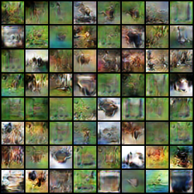
(a) $\epsilon_{\text{Adam}}=1\times 10^{-8}$

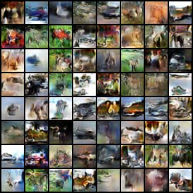
(b) $\epsilon_{\text{Adam}}=1\times 10^{-7}$

Figure 9: Qualitative comparison of generated CIFAR-10 samples under two different $\epsilon_{\text{Adam}}$ hyperparameter settings. Tuning $\epsilon_{\text{Adam}}$ affects GAN training. Zoom in for better viewing.

Appendix G Frequency of runs diverging on CIFAR-10 on three random restarts

We repeat the experiment in Figure 2 of the main paper for settings B ($\alpha=0.0002,~{}\beta_{1}=0.5,~{}\beta_{2}=0.999,~{}n_{\text{dis}}=1$), C ($\alpha=0.001,~{}\beta_{1}=0.5,~{}\beta_{2}=0.999,~{}n_{\text{dis}}=5$) and D ($\alpha=0.001,~{}\beta_{1}=0.9,~{}\beta_{2}=0.999,~{}n_{\text{dis}}=5$) that have aggressive training settings over 3 random restarts. We call a run “diverging” when the FID $\geq 40$ on CIFAR-10. Table 8 summarizes the number of diverging runs out of 3 random restarts.

Evidently, GraND-GAN and GraNC-GAN have the least number of runs that diverged in 3 random restarts across settings B, C and D. SNGAN comes close but diverges $3/3$ times for setting B when $n_{\text{dis}}=1$. WGAN-GP performs poorly across random restarts for B, C and D. NSGAN-GP$\dagger$ diverges $3/3$ times for settings B and C.

Appendix H Qualitative Results

Figures 12, 13, 14, 10 and 11 present a sample of images generated by different methods for CIFAR-10, CIFAR-100, STL-10, LSUN-Bedrooms and CelebA, respectively. We compare the results of our methods qualitatively with the baselines (NSGAN, WGAN-GP, SNGAN) and the best model of the modified baselines (NSGAN-GP$\dagger$ where $\dagger$ represents an adjusted Lipschitz constraint to match the piecewise Lipschitz constant of our methods).

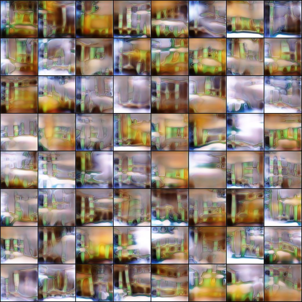
(a) NSGAN

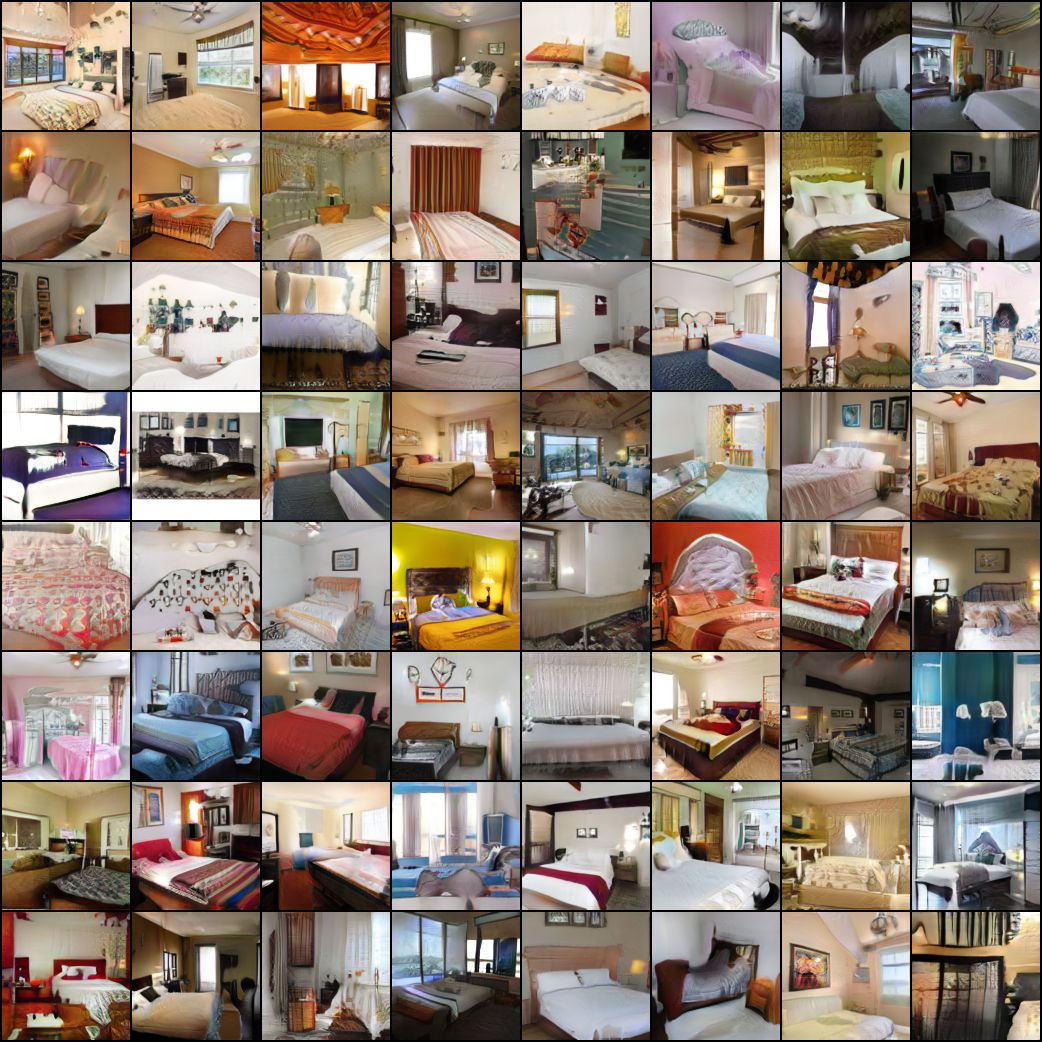
(b) WGAN-GP

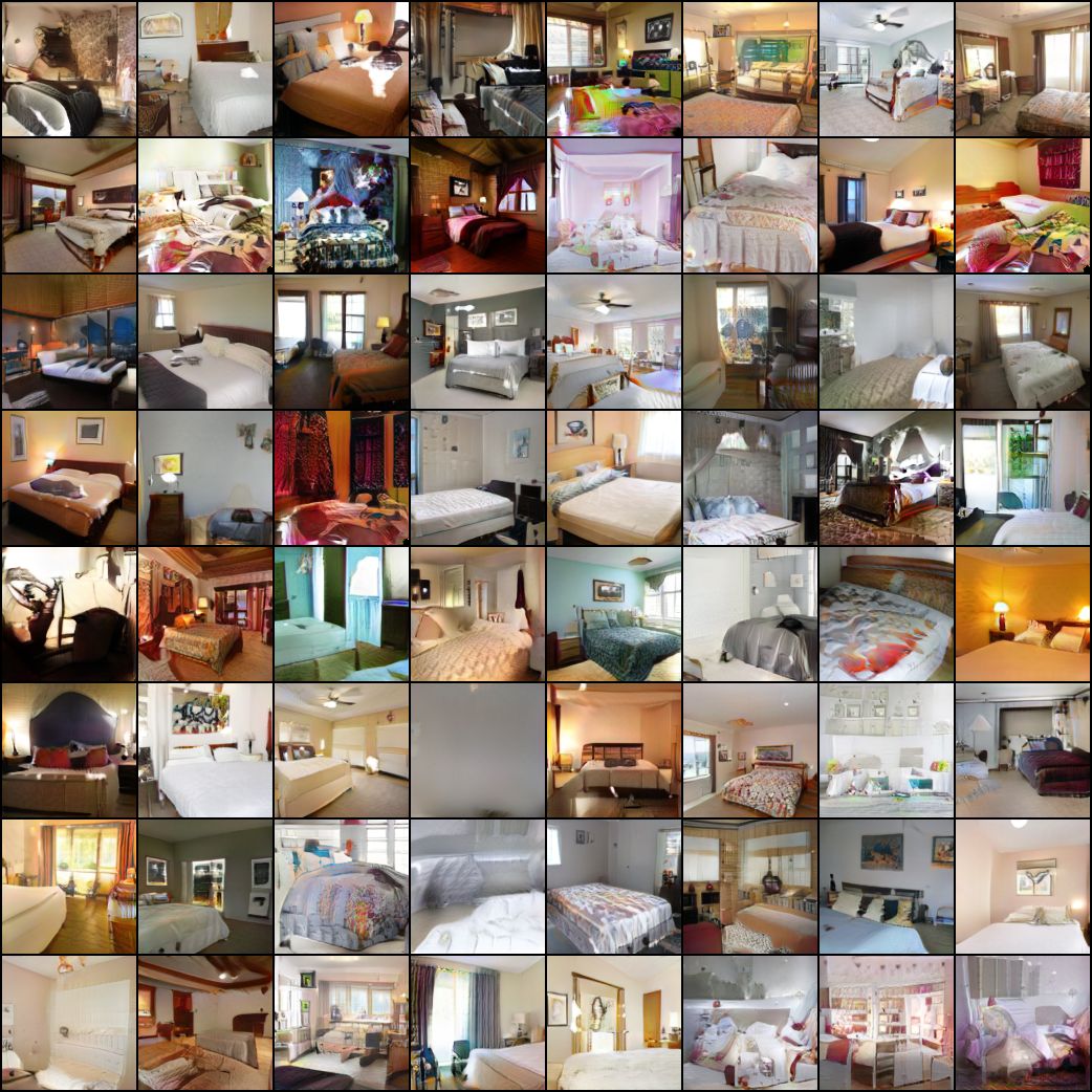
(c) SNGAN

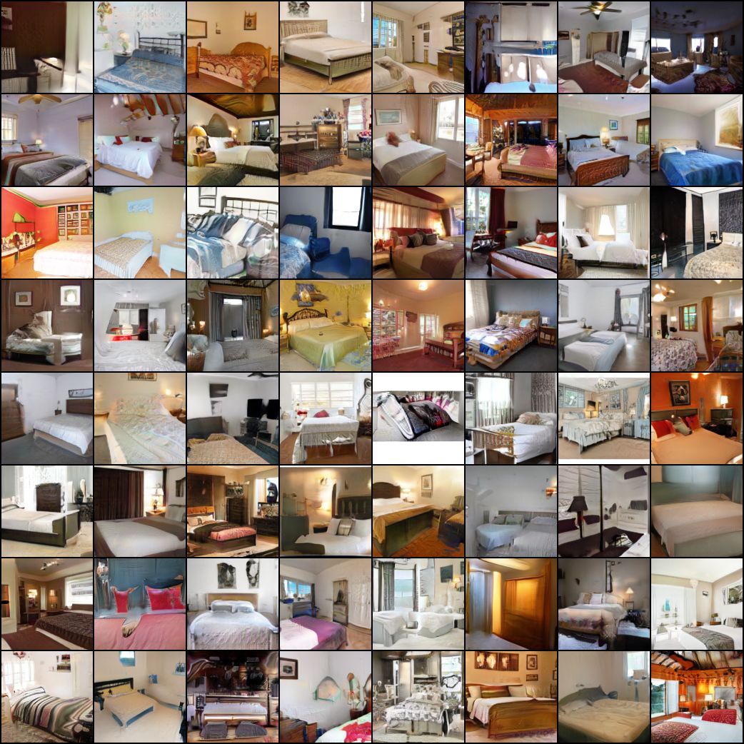
(d) NSGAN-GP$\dagger$

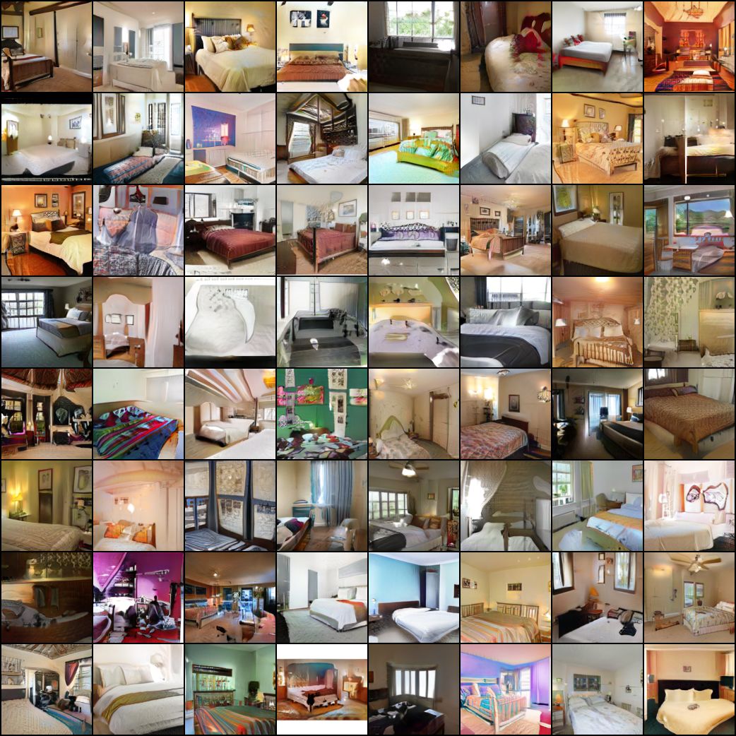
(e) GraND-GAN

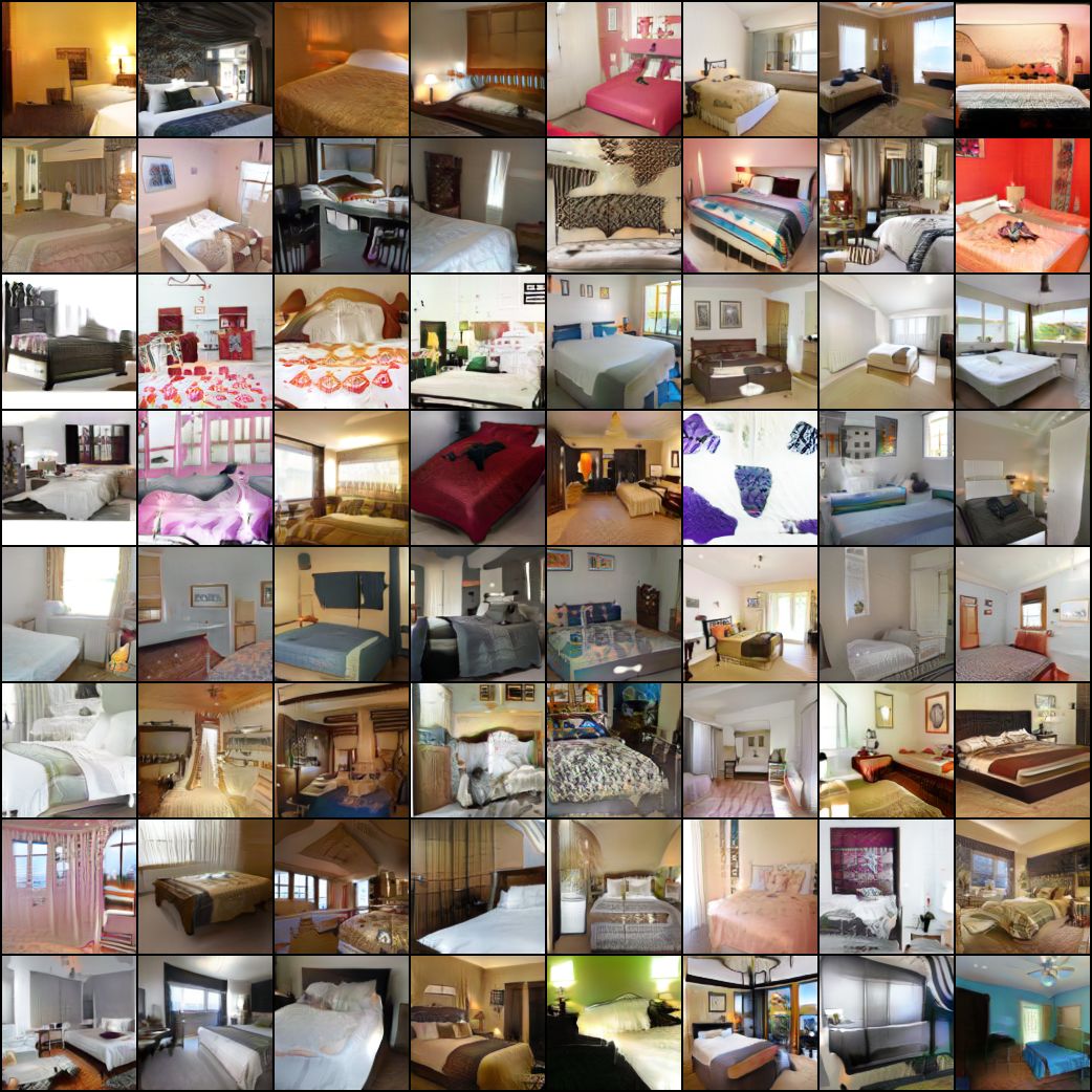
(f) GraNC-GAN

Figure 10: Qualitative results on LSUN-Bedrooms across different models, including baselines (NSGAN, WGAN-GP, SNGAN), the best performing modified baseline (NSGAN-GP$\dagger$) and our methods (GraND-GAN and GraNC-GAN). Zoom in for better viewing.

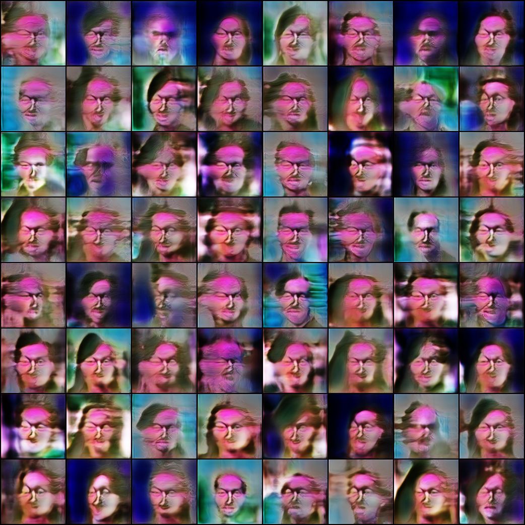
(a) NSGAN

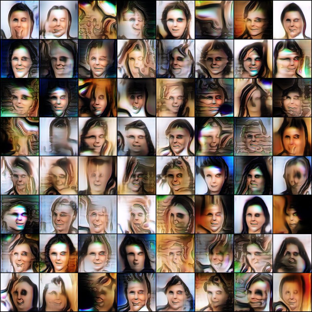
(b) WGAN-GP

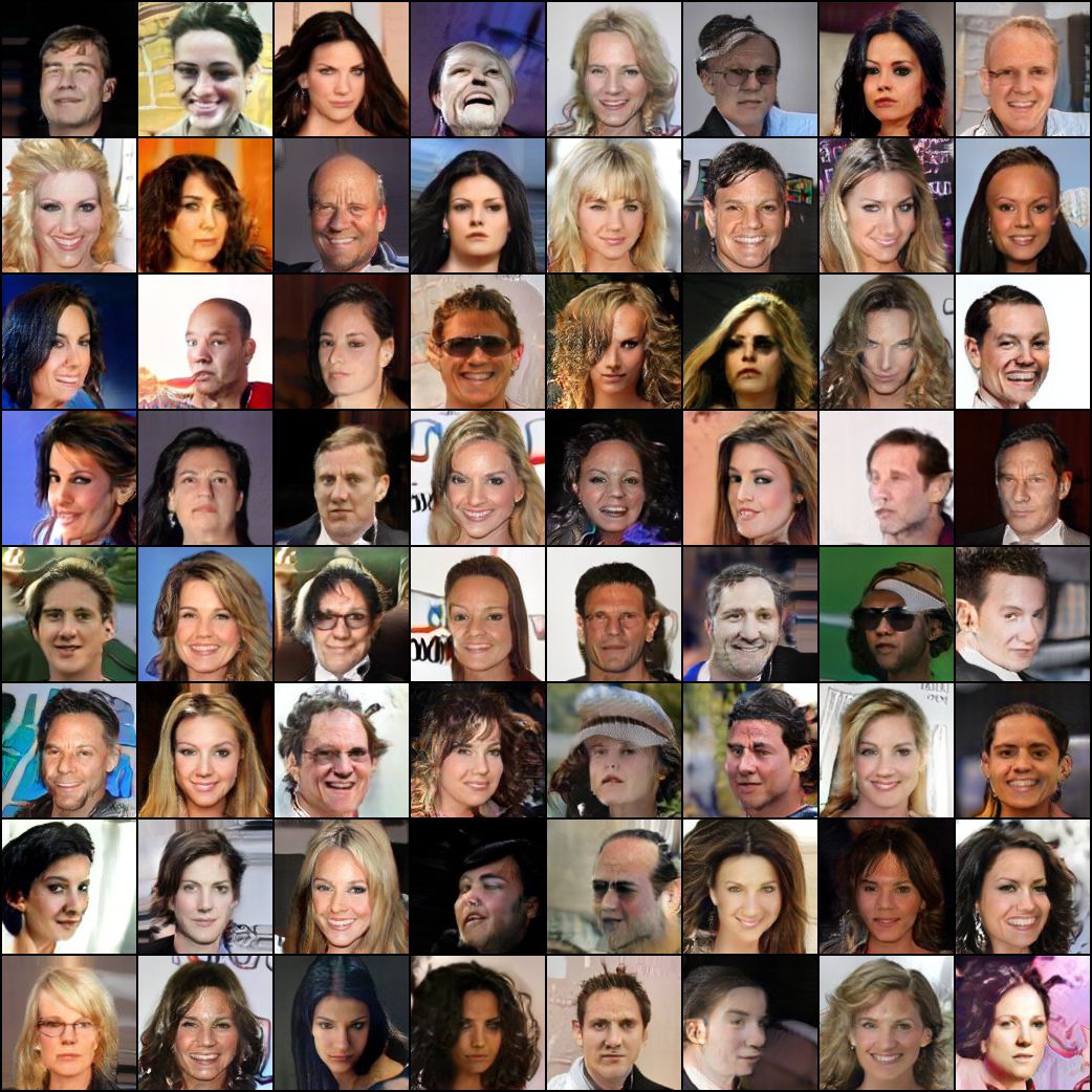
(c) SNGAN

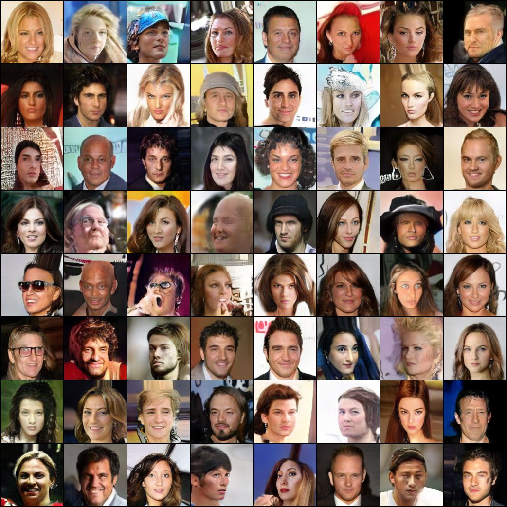
(d) NSGAN-GP$\dagger$

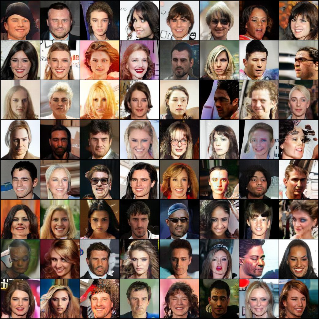
(e) GraND-GAN

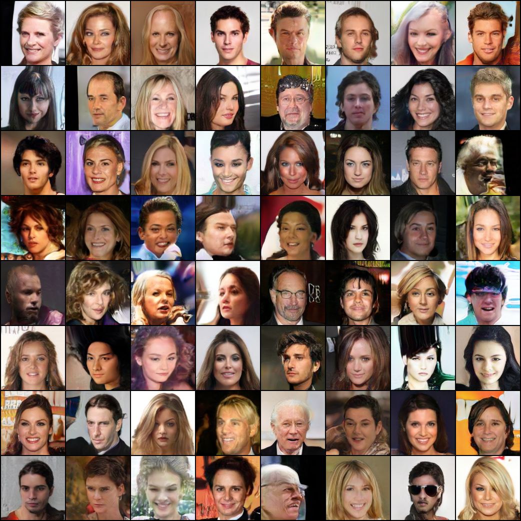
(f) GraNC-GAN

Figure 11: Qualitative results on CelebA across different models, including baselines (NSGAN, WGAN-GP, SNGAN), the best performing modified baseline (NSGAN-GP$\dagger$) and our methods (GraND-GAN and GraNC-GAN). Zoom in for better viewing.

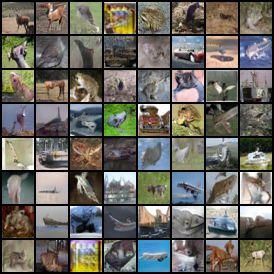
(a) NSGAN

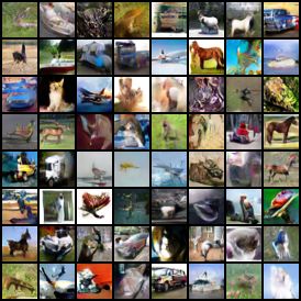
(b) WGAN-GP

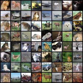
(c) SNGAN

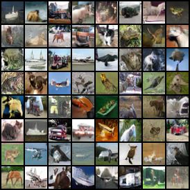
(d) NSGAN-GP$\dagger$

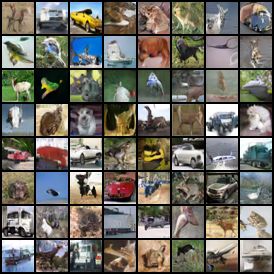
(e) GraND-GAN

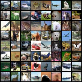
(f) GraNC-GAN

Figure 12: Qualitative results on CIFAR-10 across different models, including baselines (NSGAN, WGAN-GP, SNGAN), the best performing modified baseline (NSGAN-GP$\dagger$) and our methods (GraND-GAN and GraNC-GAN). Zoom in for better viewing.

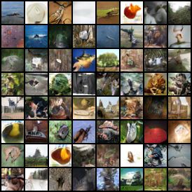
(a) NSGAN

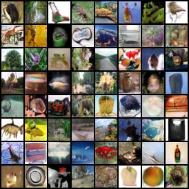
(b) WGAN-GP

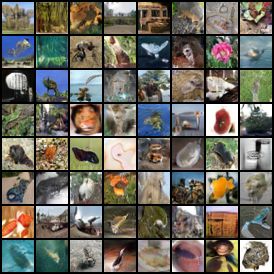
(c) SNGAN

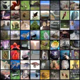
(d) NSGAN-GP$\dagger$

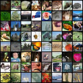
(e) GraND-GAN

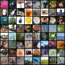
(f) GraNC-GAN

Figure 13: Qualitative results on CIFAR-100 across different models, including baselines (NSGAN, WGAN-GP, SNGAN), the best performing modified baseline (NSGAN-GP$\dagger$) and our methods (GraND-GAN and GraNC-GAN). Zoom in for better viewing.

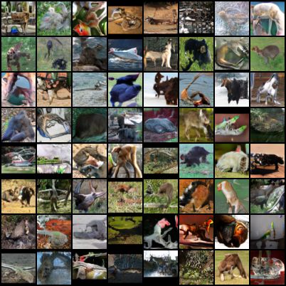
(a) NSGAN

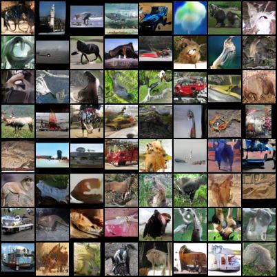
(b) WGAN-GP

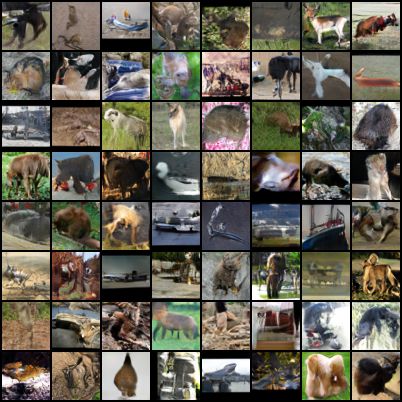
(c) SNGAN

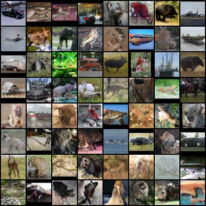
(d) NSGAN-GP$\dagger$

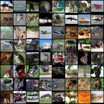
(e) GraND-GAN

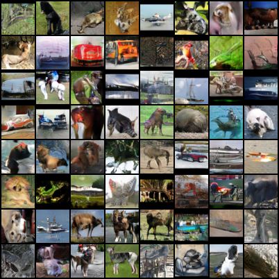
(f) GraNC-GAN

Figure 14: Qualitative results on STL-10 across different models, including baselines (NSGAN, WGAN-GP, SNGAN), the best performing modified baseline (NSGAN-GP$\dagger$) and our methods (GraND-GAN and GraNC-GAN). Zoom in for better viewing.

Appendix I Soft versus Hard Hinge Performance

We tested GraNC-GAN on both soft and hard hinge losses (recalling that the soft hinge loss is obtained by replacing the ReLU non-linearity in the standard hard hinge loss with the softplus activation). On LSUN, GraNC-GAN struggles to converge with hard hinge, while it outperforms SNGAN with soft hinge loss. Moreover, if one lowers the LRs on LSUN (to be those used by GraNC-GAN on CelebA; see §A), the soft hinge version performs better by ${\sim}$6 FID (specifically, 20.2 vs. 26.3). On CelebA, using hard hinge resulted in an FID of 14, two points higher than that obtained via soft hinge (12), as displayed in the main paper. Altogether, these suggest the soft hinge loss is generally more performant and stable than the standard hard hinge function, at least for GraN. Previous works, such as SNGAN, also note such instabilities across different loss functions, and, therefore, switch from the Wasserstein loss to the (hard) hinge loss in their work. In our case, soft hinge loss was found to work the best.

Appendix J Effect of $\epsilon_{\text{Adam}}$ in the Adam update on GAN training

To illustrate a qualitative effect of tuning $\epsilon_{\text{Adam}}$ in the Adam update on training GANs, we train GraNC-GAN on CIFAR-10 with Hinge loss for 1000 iterations, fixing the Lipschitz constant $\mathcal{K}=1$. We train two models, one with $\epsilon_{\text{Adam}}=1\times 10^{-8}$ (default value) and another model with $\epsilon_{\text{Adam}}=1\times 10^{-7}$ (i.e., $10\times$ larger than the default). Figure 9 show the qualitative results of a few examples sampled from the generators.

As noted in the main paper, tuning the Lipschitz constant $\mathcal{K}$ has an effect that is equivalent to changing $\epsilon_{\text{Adam}}$. Figure 9 qualitatively demonstrates that tuning $\epsilon_{\text{Adam}}$ (or $\mathcal{K}$, in effect) affects GAN training considerably.

Appendix K Stability of Modern GANs

Recent families of GANs, including those based on BigGAN [6] and StyleGAN [18], have achieved unprecedented synthesis results; yet, they are not immune from instability issues. BigGAN devotes a significant portion of their paper to understanding stability (see, e.g., Sections 4.1 and 4.2 on “characterizing instability”). Furthermore, they note that “it is possible to enforce stability by strongly constraining D, but doing so incurs a dramatic cost in performance.” Instability persists even within more recent methods that are based on BigGAN, such as U-net GAN [37], which experiences ${\sim}40\%$ of its runs failing. While StyleGAN does not present a stability analysis, their network relies heavily on progressive growing [17] for stability, which induces artifacts (and additional training complexity) addressed in follow-up work (StyleGANv2 [19]). Similarly, MSG-GAN [16] demonstrates improved stability of its technique over progressive growing. In other words, despite steady improvements, GAN stability remains a significant challenge, even for modern architectures. See also [40] for a recent survey of stabilization techniques.

References

- [1] Cem Anil, James Lucas, and Roger Grosse. Sorting out lipschitz function approximation. In International Conference on Machine Learning, pages 291–301. PMLR, 2019.
- [2] Martin Arjovsky and Léon Bottou. Towards principled methods for training generative adversarial networks. arXiv preprint arXiv:1701.04862, 2017.
- [3] Martin Arjovsky, Soumith Chintala, and Léon Bottou. Wasserstein generative adversarial networks. In International conference on machine learning, pages 214–223. PMLR, 2017.
- [4] David Berthelot, Thomas Schumm, and Luke Metz. Began: Boundary equilibrium generative adversarial networks. arXiv preprint arXiv:1703.10717, 2017.
- [5] Mikołaj Bińkowski, Dougal J Sutherland, Michael Arbel, and Arthur Gretton. Demystifying mmd gans. arXiv preprint arXiv:1801.01401, 2018.
- [6] Andrew Brock, Jeff Donahue, and Karen Simonyan. Large scale gan training for high fidelity natural image synthesis. arXiv preprint arXiv:1809.11096, 2018.
- [7] Eric R Chan, Marco Monteiro, Petr Kellnhofer, Jiajun Wu, and Gordon Wetzstein. pi-gan: Periodic implicit generative adversarial networks for 3d-aware image synthesis. arXiv preprint arXiv:2012.00926, 2020.
- [8] Adam Coates, Andrew Ng, and Honglak Lee. An analysis of single-layer networks in unsupervised feature learning. In Proceedings of the fourteenth international conference on artificial intelligence and statistics, pages 215–223. JMLR Workshop and Conference Proceedings, 2011.
- [9] Arnab Ghosh, Viveka Kulharia, Vinay P Namboodiri, Philip HS Torr, and Puneet K Dokania. Multi-agent diverse generative adversarial networks. In Proceedings of the IEEE conference on computer vision and pattern recognition, pages 8513–8521, 2018.
- [10] Gene H Golub and Charles F Van Loan. Matrix computations (fourth edition). JHU press, 2013.
- [11] Xinyu Gong, Shiyu Chang, Yifan Jiang, and Zhangyang Wang. Autogan: Neural architecture search for generative adversarial networks. In Proceedings of the IEEE/CVF International Conference on Computer Vision, pages 3224–3234, 2019.
- [12] Ian J Goodfellow, Jean Pouget-Abadie, Mehdi Mirza, Bing Xu, David Warde-Farley, Sherjil Ozair, Aaron Courville, and Yoshua Bengio. Generative adversarial networks. arXiv preprint arXiv:1406.2661, 2014.
- [13] Ishaan Gulrajani, Faruk Ahmed, Martin Arjovsky, Vincent Dumoulin, and Aaron Courville. Improved training of Wasserstein gans. In Proceedings of the 31st International Conference on Neural Information Processing Systems, pages 5769–5779, 2017.
- [14] Martin Heusel, Hubert Ramsauer, Thomas Unterthiner, Bernhard Nessler, and Sepp Hochreiter. Gans trained by a two time-scale update rule converge to a local nash equilibrium. In Proceedings of the 31st International Conference on Neural Information Processing Systems, NIPS’17, page 6629–6640, Red Hook, NY, USA, 2017. Curran Associates Inc.
- [15] Sergey Ioffe and Christian Szegedy. Batch normalization: Accelerating deep network training by reducing internal covariate shift. In International conference on machine learning, pages 448–456. PMLR, 2015.
- [16] Animesh Karnewar and Oliver Wang. Msg-gan: Multi-scale gradients for generative adversarial networks. In Proceedings of the IEEE/CVF Conference on Computer Vision and Pattern Recognition, pages 7799–7808, 2020.
- [17] Tero Karras, Timo Aila, Samuli Laine, and Jaakko Lehtinen. Progressive growing of gans for improved quality, stability, and variation. arXiv preprint arXiv:1710.10196, 2017.
- [18] Tero Karras, Samuli Laine, and Timo Aila. A style-based generator architecture for generative adversarial networks. In Proceedings of the IEEE/CVF Conference on Computer Vision and Pattern Recognition, pages 4401–4410, 2019.
- [19] Tero Karras, Samuli Laine, Miika Aittala, Janne Hellsten, Jaakko Lehtinen, and Timo Aila. Analyzing and improving the image quality of stylegan. In Proceedings of the IEEE/CVF Conference on Computer Vision and Pattern Recognition, pages 8110–8119, 2020.
- [20] Diederik P Kingma and Jimmy Ba. Adam: A method for stochastic optimization. arXiv preprint arXiv:1412.6980, 2014.
- [21] Alex Krizhevsky. Learning multiple layers of features from tiny images. Technical report, 2009.
- [22] Kwot Sin Lee and Christopher Town. Mimicry: Towards the reproducibility of gan research. CVPR Workshop on AI for Content Creation, 2020.
- [23] Qiyang Li, Saminul Haque, Cem Anil, James Lucas, Roger B Grosse, and Joern-Henrik Jacobsen. Preventing gradient attenuation in lipschitz constrained convolutional networks. In H. Wallach, H. Larochelle, A. Beygelzimer, F. d Alché-Buc, E. Fox, and R. Garnett, editors, Advances in Neural Information Processing Systems, volume 32, pages 15390–15402. Curran Associates, Inc., 2019.
- [24] Jae Hyun Lim and Jong Chul Ye. Geometric gan. arXiv preprint arXiv:1705.02894, 2017.
- [25] David B. Lindell, Julien N. P. Martel, and Gordon Wetzstein. Autoint: Automatic integration for fast neural volume rendering. In Proceedings of the IEEE/CVF Conference on Computer Vision and Pattern Recognition (CVPR), pages 14556–14565, June 2021.
- [26] Ziwei Liu, Ping Luo, Xiaogang Wang, and Xiaoou Tang. Deep learning face attributes in the wild. In Proceedings of International Conference on Computer Vision (ICCV), December 2015.
- [27] Xudong Mao, Qing Li, Haoran Xie, Raymond YK Lau, Zhen Wang, and Stephen Paul Smolley. Least squares generative adversarial networks. In Proceedings of the IEEE international conference on computer vision, pages 2794–2802, 2017.
- [28] Lars Mescheder, Andreas Geiger, and Sebastian Nowozin. Which training methods for gans do actually converge? In International conference on machine learning, pages 3481–3490. PMLR, 2018.
- [29] Luke Metz, Ben Poole, David Pfau, and Jascha Sohl-Dickstein. Unrolled generative adversarial networks. In 5th International Conference on Learning Representations, ICLR 2017, 2017.
- [30] Takeru Miyato, Toshiki Kataoka, Masanori Koyama, and Yuichi Yoshida. Spectral normalization for generative adversarial networks. In International Conference on Learning Representations, 2018.
- [31] Jeeseung Park and Younggeun Kim. Styleformer: Transformer based generative adversarial networks with style vector. arXiv preprint, arXiv:2106.07023, 2021.
- [32] Adam Paszke, Sam Gross, Francisco Massa, Adam Lerer, James Bradbury, Gregory Chanan, Trevor Killeen, Zeming Lin, Natalia Gimelshein, Luca Antiga, Alban Desmaison, Andreas Kopf, Edward Yang, Zachary DeVito, Martin Raison, Alykhan Tejani, Sasank Chilamkurthy, Benoit Steiner, Lu Fang, Junjie Bai, and Soumith Chintala. Pytorch: An imperative style, high-performance deep learning library. In H. Wallach, H. Larochelle, A. Beygelzimer, F. d’Alché Buc, E. Fox, and R. Garnett, editors, Advances in Neural Information Processing Systems 32, pages 8024–8035. Curran Associates, Inc., 2019.
- [33] Henning Petzka, Asja Fischer, and Denis Lukovnicov. On the regularization of wasserstein gans. arXiv preprint arXiv:1709.08894, 2017.
- [34] Kevin Roth, Aurelien Lucchi, Sebastian Nowozin, and Thomas Hofmann. Stabilizing training of generative adversarial networks through regularization. arXiv preprint arXiv:1705.09367, 2017.
- [35] Tim Salimans, Ian Goodfellow, Wojciech Zaremba, Vicki Cheung, Alec Radford, and Xi Chen. Improved techniques for training gans. arXiv preprint arXiv:1606.03498, 2016.
- [36] Tim Salimans and Diederik P Kingma. Weight normalization: a simple reparameterization to accelerate training of deep neural networks. In Proceedings of the 30th International Conference on Neural Information Processing Systems, pages 901–909, 2016.
- [37] Edgar Schonfeld, Bernt Schiele, and Anna Khoreva. A u-net based discriminator for generative adversarial networks. In Proceedings of the IEEE/CVF Conference on Computer Vision and Pattern Recognition, pages 8207–8216, 2020.
- [38] Hung-Yu Tseng, Lu Jiang, Ce Liu, Ming-Hsuan Yang, and Weilong Yang. Regularizing generative adversarial networks under limited data. In Proceedings of the IEEE/CVF Conference on Computer Vision and Pattern Recognition, pages 7921–7931, 2021.
- [39] Xiang Wei, Boqing Gong, Zixia Liu, Wei Lu, and Liqiang Wang. Improving the improved training of wasserstein gans: A consistency term and its dual effect. In International Conference on Learning Representations (ICLR), 2018.
- [40] Maciej Wiatrak, Stefano V Albrecht, and Andrew Nystrom. Stabilizing generative adversarial networks: A survey. arXiv preprint arXiv:1910.00927, 2019.
- [41] Yi-Lun Wu, Hong-Han Shuai, Zhi-Rui Tam, and Hong-Yu Chiu. Gradient normalization for generative adversarial networks. In Proceedings of the IEEE/CVF International Conference on Computer Vision (ICCV), pages 6373–6382, October 2021.
- [42] Fisher Yu, Yinda Zhang, Shuran Song, Ari Seff, and Jianxiong Xiao. Lsun: Construction of a large-scale image dataset using deep learning with humans in the loop. arXiv preprint arXiv:1506.03365, 2015.
- [43] Han Zhang, Ian Goodfellow, Dimitris Metaxas, and Augustus Odena. Self-attention generative adversarial networks. In International conference on machine learning, pages 7354–7363. PMLR, 2019.
- [44] Shengyu Zhao, Zhijian Liu, Ji Lin, Jun-Yan Zhu, and Song Han. Differentiable augmentation for data-efficient gan training. In Conference on Neural Information Processing Systems (NeurIPS), 2020.
- [45] Zhiming Zhou, Jiadong Liang, Yuxuan Song, Lantao Yu, Hongwei Wang, Weinan Zhang, Yong Yu, and Zhihua Zhang. Lipschitz generative adversarial nets. In International Conference on Machine Learning, pages 7584–7593. PMLR, 2019.
- [46] Peizhen Zhu and Andrew V Knyazev. Angles between subspaces and their tangents. arXiv preprint arXiv:1209.0523, 2012.
- [47] Dongmian Zou, Radu Balan, and Maneesh Singh. On lipschitz bounds of general convolutional neural networks. IEEE Transactions on Information Theory, 66(3):1738–1759, 2019.