OU-HEP-211130

Comparison of SUSY spectra generators for
natural SUSY and string landscape predictions
Howard Baer^1,2, Vernon Barger² and Dakotah Martinez^1
1Homer L. Dodge Department of Physics and Astronomy,
University of Oklahoma, Norman, OK 73019, USA
²Department of Physics, University of Wisconsin, Madison, WI 53706 USA

Models of natural supersymmetry give rise to a weak scale $m_{weak}\sim m_{W,Z,h}\sim 100$ GeV without any (implausible) finetuning of independent contributions to the weak scale. These models, which exhibit radiatively driven naturalness (RNS), are expected to arise from statistical analysis of the string landscape wherein large soft terms are favored, but subject to a not-too-large value of the derived weak scale in each pocket universe of the greater multiverse. The string landscape picture then predicts, using the Isajet SUSY spectra generator Isasugra, a statistical peak at $m_{h}\sim 125$ GeV with sparticles generally beyond current LHC search limits. In this paper, we investigate how well these conclusions hold up using other popular spectra generators: SOFTSUSY, SPHENO and SUSPECT (SSS). We built a computer code DEW4SLHA which operates on SUSY Les Houches Accord files to calculate the associated electroweak naturalness measure $\Delta_{EW}$. The SSS generators tend to yield a Higgs mass peak $\sim 125-127$ GeV with a superparticle mass spectra rather similar to that generated by Isasugra. In an Appendix, we include loop corrections to $\Delta_{EW}$ in a more standard notation.

1 Introduction

Supersymmetrization of the Standard Model (SM) elegantly solves the gauge hierarchy problem (stabilizing the newly discovered Higgs boson mass under quantum corrections) but at the expense of including a host of new matter states, the so-called superpartners. Early expectations from naturalness predicted superpartners at or around the weak scale[1, 2, 3, 4]. For instance, the naturalness upper bound for the gluino was predicted (under the naturalness measure $\Delta_{BG}\lesssim 30$) to be $m_{\tilde{g}}\lesssim 400$ GeV. In contrast, the current mass limits from LHC Run 2 searches with 139 fb^-1 claim $m_{\tilde{g}}\gtrsim 2.25$ TeV[5, 6]. The yawning gap between the weak scale and the superpartner mass scale– the Little Hierarchy Problem (LHP)[7]– has lead many authors to conclude[8, 9, 10] that the weak scale supersymmetry[11] hypothesis is under intense pressure, and possibly even excluded.

However, it has been pointed out that the resolution to the LHP lies instead in that conventional early measures of naturalness over-estimated the finetuning[12, 13, 14]. The BG log derivative measure[2], $\Delta_{BG}\equiv max_{i}|\frac{\partial\log m_{Z}^{2}}{\partial\log p_{i}}|$ where the $p_{i}$ are fundamental parameters of the low energy effective field theory (EFT), depends strongly on what one assumes are independent parameters. To derive the bounds in Ref’s [1, 2, 3, 4], the authors adopted common scalar masses $m_{0}$, gauginos masses $m_{1/2}$ and $A$-terms as independent parameters. However, in more ultraviolet complete theories, such as string theory, these parameters are all correlated. Adopting correlated soft terms then greatly reduces the amount of finetuning which is calculated, often by 1-2 orders of magnitude. An alternative measure $\Delta_{HS}\equiv\delta m_{H_{u}}^{2}/m_{h}^{2}$, (which is inconsistent with $\Delta_{BG}$ in that it splits $m_{H_{u}}^{2}(weak)$ into $m_{H_{u}}^{2}(HS)+\delta m_{H_{u}}^{2}$ which destroys the focus point behavior inherent in $\Delta_{BG}$) discards RG contributions which show the interdependence of $m_{H_{u}}^{2}$ and $\delta m_{H_{u}}^{2}$.

An alternative measure for naturalness $\Delta_{EW}$ was proposed in [15, 16] based on the notion of practical naturalness[17]: that all independent contributions to an observable ${\cal O}$ should be comparable to or less than ${\cal O}$. For instance, if ${\cal O}=o_{1}+\cdots+o_{n}$ where the $o_{i}$ are independent contributions to ${\cal O}$, and if $o_{1}\gg{\cal O}$, then some other unrelated contribution would have been a huge opposite sign contribution of precisely the right value such as to maintain ${\cal O}$ at its measured value. Such finetunings, while logically possible, are thought to be highly implausible unless the contributions $o_{i}$ are related by some symmetry, in which case they would not actually be independent. Practical naturalness has been successfully applied for instance by Gaillard and Lee in the case of the $K_{L}-K_{S}$ mass difference to correctly predict the value of the charm quark mass[18]. It is also closely related to predictivity in physical theories in that missing contributions to an observable, such as higher order corrections in perturbation theory, should be (hopefully) small so that leading order terms provide a reliable estimate to any perturbatively calculated observable.

The minimization conditions for the MSSM Higgs potential allows one to relate the observed value of the weak scale to terms in the minimal supersymmetric standard model (MSSM) Lagrangian:

$$m_{Z}^{2}/2=\frac{(m_{H_{d}}^{2}+\Sigma_{d}^{d})-(m_{H_{u}}^{2}+\Sigma_{u}^{u})\tan^{2}\beta}{\tan^{2}\beta-1}-\mu^{2}$$ (1)

where $m_{H_{u}}^{2}$ and $m_{H_{d}}^{2}$ are Higgs sector soft breaking masses, $\mu$ is the (SUSY-conserving) $\mu$ parameter and $\tan\beta=v_{u}/v_{d}$ is the ratio of Higgs field vacuum expectation values. The $\Sigma_{d}^{d}$ and $\Sigma_{u}^{u}$ terms contain a variety of loop corrections to the Higgs potential and are detailed in Ref. [16] in the notation of Weak Scale Supersymmetry (WSS)[11] and given in the Appendix of this paper in the more standard notation from S. P. Martin[19]. The most important of the loop corrections typically comes from the top-squark sector, $\Sigma_{u}^{u}(\tilde{t}_{1,2})$. Note that all contributions in Eq. 1 are evaluated at the weak scale typically taken as $Q^{2}=m_{\tilde{t}_{1}}m_{\tilde{t}_{2}}$ such as to minimize the logs which are present in the $\Sigma_{u}^{u}(\tilde{t}_{1,2})$ contributions.

The $\Delta_{EW}$ measure is defined as

$$\Delta_{EW}\equiv|{\rm largest\ contribution\ to\ RHS\ of\ Eq.~{}\ref{eq:mzs}}|/(m_{Z}^{2}/2).$$ (2)

One can quickly read off the consequences for a low value of $\Delta_{EW}$:

• $m_{H_{u}}^{2}$, which in the decoupling limit functions like the SM Higgs doublet and gives mass to the $W$, $Z$ and $h$ bosons, must be driven under radiative EWSB to small negative values, a condition known as radiatively-driven naturalness (RNS). Thus, electroweak symmetry is barely broken.

• The $\mu$ parameter, which feeds mass to the $W$, $Z$ and $h$ bosons as well as to the higgsinos, must be within a factor of several of $m_{W,Z,h}\sim 100$ GeV.

• $m_{A}\sim m_{H_{d}}$ in the decoupling limit can live in the TeV regime since the contribution of $m_{H_{d}}^{2}$ is suppressed by a factor $\tan^{2}\beta$.

• Top squark contributions to the weak scale are loop suppressed and so can live in the TeV range while maintaining naturalness.

• The gluino contributes at two-loops[20] and via RG running contributions to the stop soft masses[21, 22] and so also can live in the TeV range,

• First and second generation sfermion contributions to the weak scale are via Yukawa-suppressed 1-loop terms and via 2-loop RG contributions (which are dominant)[23]. Thus, they can live in the 10-50 TeV regime which helps solve the SUSY flavor and CP problems[24].

An advantage of $\Delta_{EW}$ is that it is model independent insofar as it only depends on the weak scale sparticle and Higgs mass spectrum and not on how they are arrived at. Thus, a given spectrum will generate the same value of $\Delta_{EW}$ whether it was computed from the pMSSM or some high scale model. Also, requiring the contributions to $m_{Z}^{2}/2$ to be comparable to or less than its measured value typically corresponds to an upper limit of $\Delta_{EW}\lesssim 30$. The turn-on of finetuning for $\Delta_{EW}\gtrsim 30$ is visually displayed in Fig. 1 of Ref. [17].

While WSS seems ruled out under the older naturalness measures[1, 2, 3, 4], there is still plenty of natural parameter space left unexplored by LHC under the $\Delta_{EW}$ measure[25]. However, the $\Delta_{EW}$ measure does predict the existence of light higgsino-like EWinos $\tilde{\chi}_{1}^{\pm}$ and $\tilde{\chi}_{1,2}^{0}$ with mass $\sim 100-350$ GeV. The light higgsinos can be produced at decent rates at LHC, but owing to their small mass gaps $m_{\tilde{\chi}_{2}^{0}}-m_{\tilde{\chi}_{1}^{0}}\sim 5-10$ GeV, there is only small visible energy released in their decays, making detection a difficult[26] (but not impossible[27, 28]) prospect. The higgsino-like LSP $\tilde{\chi}_{1}^{0}$ is thermally underproduced as dark matter, leaving room for axionic dark matter as well[29].

The $\Delta_{EW}$ naturalness measure is built in to the Isajet/Isasugra[30, 31] event/spectrum generator. Also, the crucial 1-loop corrections to the Higgs potential have been calculated within the (non-standard) notation of WSS[16]. As a result, of the spectrum generators available, Isasugra has been used the most for such studies. These include sparticle mass bounds from naturalness, and parameter space limits and lucrative collider signatures from natural SUSY. However, a variety of other SUSY/Higgs spectra generators are available, including SUSPECT[32], SOFTSUSY[33] and SPHENO[34]. Some special Higgs spectrum calculators include FeynHIGGS[35] and SUSYHD[36] and others[37]. Thus, it would be useful to know how other spectrum generators compare to Isasugra in their natural SUSY spectra. For this reason, we have built a computer code DEW4SLHA which operates on a SUSY Les Houches Accord file (SLHA)[38] which is the standard output of spectrum generators. The program computes the associated value of $\Delta_{EW}$ and all the various contributions. In Sec. 2 of this paper, we introduce the code DEW4SLHA along with pointers on its accessibility.

While natural SUSY is highly interesting in its own right, some authors maintain that naturalness should cede ground to the emergent landscape/multiverse picture of string theory: if the cosmological constant $\Lambda_{cc}$ is finetuned to tiny values via anthropic selection in the multiverse, then why not also the weak scale? There is expected to be a statistical pull to large soft SUSY breaking terms via a power law[39, 40, 41] or log distribution[42] in the landscape of string theory vacua. However, one of the most important predictions of SUSY theories is the magnitude of the weak scale $m_{weak}$. Agrawal et al.[43, 44] have shown that if the pocket universe value of the weak scale is greater than a factor of 2-5 times our universe’s measured value, then complex nuclei, and hence atoms as we know them, would not arise. Now in a subset of vacua with the MSSM as low energy EFT but with variable soft terms, then absent finetuning, the pocket universe value of the weak scale $m_{weak}^{PU}$ will nearly be the maximal contribution to the RHS of Eq. 1. Thus, a value $m_{Z}^{PU}\sim 4m_{Z}^{OU}$ corresponds to a value $\Delta_{EW}\lesssim 30$. This anthropic veto has been used along with a landscape pull to large soft terms to make statistical predictions from the string landscape for the SUSY and Higgs boson masses. It is found using Isasugra that the Higgs mass $m_{h}$ rises to a peak at $m_{h}\sim 125$ GeV while sparticles such as the lightest stop and gluino are pulled to values beyond LHC13 search limits. It would also be of interest to confirm or refute these results using other spectra/Higgs mass calculators.

Thus, in this paper we first introduce the public code DEW4SLHA in Sec. 2. In Sec. 3, we apply this code to a natural SUSY benchmark point to compare spectra from Isasugra against results from SOFTSUSY, SUSPECT and SPHENO. As such, our paper follows previous comparison work but within the context of natural SUSY and string landscape phenomenology[45, 46]. In Sec. 3, we also move beyond benchmark points to compare Higgs mass and naturalness contours in the scalar mass vs. gaugino mass parameter planes for just the SOFTSUSY spectrum generator. In Sec. 4, we use SOFTSUSY to generate statistical landscape predictions to compare against earlier work from Isasugra. A summary and conclusions are given in Sec. 5. In an Appendix A, we present expressions for the $\Sigma_{u}^{u}$ and $\Sigma_{d}^{d}$ contributions in the standard notation of S. P. Martin’s SUSY primer [19].

2 The DEW4SLHA code

A new code, DEW4SLHA, has been developed in Python 3 by D. Martinez to evaluate $\Delta_{EW}$ from any user-supplied SLHA-format output from a spectrum generator such as Isajet, SOFTSUSY, SUSPECT, or SPHENO. The standalone executable can be found at https://dew4slha.com, along with instructions on how to run the program from a Linux terminal. The source code can be found at https://github.com/Dmartinez-96/DEW-Calculator . The DEW4SLHA code uses the SLHA particle/sparticle pole masses from block MASS and the running soft term values from block MSOFT. DEW4SLHA has the capability to operate on SLHA files with a single-scale output or a grid of outputs, with the number of grid points specified by Switch 11 in the SLHA block MODSEL. In the case of the latter, DEW4SLHA extracts the values of parameters at the maximum grid scale and computes DEW using the parameters at this scale. The computational routine of the program follows the equations presented in the Appendix A and then orders the 44 1-loop contributions to the Higgs minimization condition by magnitude. Two corrections at the 2-loop level are included in the routine to include the effects of the gluino mass on the DEW measure[20]. Similar codes have been developed but are not to our knowledge publicly available[47, 48].

3 Natural SUSY benchmark points

Using the code DEW4SLHA, we can now compare spectra generated from the various spectra calculators for a particular natural SUSY benchmark point. For the BM point, we adopt the two-extra-parameter non-universal Higgs model (NUHM2)[49, 50] with input parameters

$$m_{0},\ m_{1/2},\ A_{0},\ \tan\beta,\ \mu,\ m_{A}$$ (3)

where we have traded the high scale Higgs soft masses $m_{H_{u}}^{2}$ and $m_{H_{d}}^{2}$ for the more convenient weak scale parameters $\mu$ and $m_{A}$. Then we adopt the benchmark parameter values $m_{0}=5$ TeV, $m_{1/2}=1.2$ TeV, $A_{0}=-8$ TeV, $\tan\beta=10$, $\mu=200$ GeV and $m_{A}=2$ TeV. A pictorial representation of the spectra using SOFTSUSY is shown in Fig. 1 where we see that indeed the higgsinos and Higgs boson $h$ lie in the $100-200$ GeV range whilst the top-squarks and gluino live in the several TeV regime.

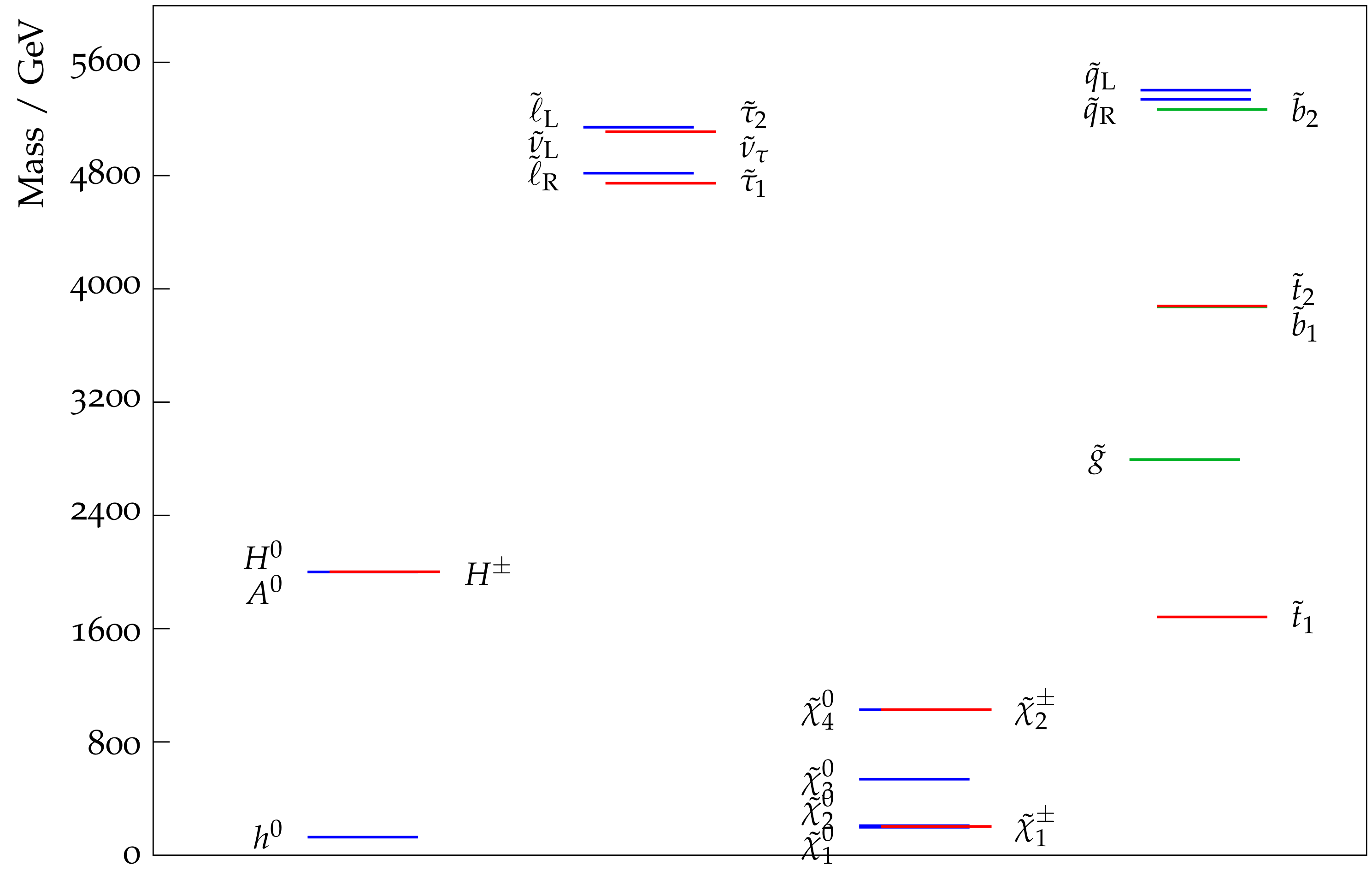
Figure 1: Sparticle and Higgs mass spectra for a natural SUSY benchmark point from SOFTSUSY.

In Table 1, we list the mass spectra and $\Delta_{EW}$ values from each of four spectra generators. For ISAJET, we use version 7.88[30] while for SUSPECT we use version 2.51[32]. For SOFTSUSY, we use version 4.1.10[33] including two-loop corrections to $m_{\tilde{g}}$ and the default two-loop corrections to $m_{h}$. We use SPHENO version 4.0.4[34] with MSSM-to-SM matching at scale $Q=m_{SUSY}=\sqrt{m_{\tilde{t}_{1}}m_{\tilde{t}_{2}}}$. In contrast, SOFTSUSY imposes EFT matching at $Q=m_{Z}$ while ISAJET uses multiple scales[Baer:2005pv]. The gluino masses are all within 1.5% of each other. The naturalness parameters for three codes are all less than thirty; the outlier here is SPHENO where also the light top squark mass $m_{\tilde{t}_{1}}$ is somewhat higher than the other codes. Here, the top squark masses are highly sensitive to mixing which comes from the weak scale value of $A_{t}$ and indeed the values of $A_{t}(Q)$ for Isasugra/SOFTSUSY/SUSPECT/SPHENO are -4898/-4830/-4894/-5090 GeV, respectively. Thus, SPHENO has slightly more stop mixing than the other codes which increases $\Delta_{EW}$ somewhat. Another difference comes from the value of $m_{h}$ generated: both SOFTSUSY and SUSPECT generate $m_{h}\sim 127.4$ GeV whilst SPHENO generates $m_{h}=125.2$ GeV and Isasugra generates $m_{h}=124.7$ GeV. It can be remarked that Isasugra has the least sophisticated light Higgs mass calculation, and includes only third generation sparticle 1-loop contributions to $m_{h}$. Another feature is that the Isasugra value of $m_{\tilde{\chi}_{1}^{\pm}}$ is about six GeV higher than SOFTSUSY and SUSPECT while the SPHENO is six GeV lower. These values depend sensitively on the scale choice at which each EWino mass is calculated. For instance, Isasugra uses the Pierce et al. (PBMZ)[51] recipe to calculate each mass separately at each mass scale.

parameter	Isasugra	SOFTSUSY	SUSPECT	SPHENO
$m_{\tilde{g}}$	2830.7	2794.3	2838.6	2827.6
$m_{\tilde{u}_{L}}$	5440.3	5403.2	5406.0	5412.8
$m_{\tilde{u}_{R}}$	5561.7	5521.3	5523.0	5521.8
$m_{\tilde{e}_{R}}$	4823.0	4817.3	4818.1	4825.8
$m_{\tilde{t}_{1}}$	1714.3	1682.8	1746.9	1942.1
$m_{\tilde{t}_{2}}$	3915.1	3879.0	3899.2	3947.0
$m_{\tilde{b}_{1}}$	3949.1	3871.6	3891.7	3939.1
$m_{\tilde{b}_{2}}$	5287.5	5266.4	5277.2	5281.7
$m_{\tilde{\tau}_{1}}$	4745.7	4746.1	4749.1	4757.4
$m_{\tilde{\tau}_{2}}$	5110.2	5109.7	5110.8	5107.2
$m_{\tilde{\nu}_{\tau}}$	5116.8	5108.7	5113.8	5106.2
$m_{\widetilde{\chi}^{\pm}_{2}}$	1020.2	1027.5	1030.6	1031.9
$m_{\widetilde{\chi}^{\pm}_{1}}$	209.7	203.1	203.0	197.3
$m_{\widetilde{\chi}^{0}_{4}}$	1033.5	1027.3	1031.1	1032.0
$m_{\widetilde{\chi}^{0}_{3}}$	540.1	536.4	537.2	538.1
$m_{\widetilde{\chi}^{0}_{2}}$	-208.3	-208.6	-208.7	-203.0
$m_{\widetilde{\chi}^{0}_{1}}$	197.9	197.2	197.1	191.9
$m_{h}$	124.7	127.3	127.5	125.2
$\Delta_{\rm EW}$	24.8	23.0	28.2	44.1

Table 1: Sparticle and Higgs mass spectra from four spectra generators for a natural SUSY benchmark point with $m_{0}=5$ TeV, $m_{1/2}=1.2$ TeV, $A_{0}=-8$ TeV, $\tan\beta=10$ with $\mu=200$ GeV and $m_{A}=2$ TeV.

In Table 2, we list the top 46 contributions to $\Delta_{EW}$ from each of the spectra codes. We see from line 1 that the largest contribution comes for each code from $\Sigma_{u}^{u}(\tilde{t}_{2})$ which sets the value of $\Delta_{EW}$, and where we see that SPHENO gives the largest value. The second largest contribution comes from $\Sigma_{u}^{u}(\tilde{t}_{1})$ as might be expected. The next several largest contributions come from $H_{d}$, $\mu$ and $H_{u}$ and $\Sigma_{u}^{u}(\tilde{b}_{1,2})$ although the ordering of these differs among the codes. In general, the agreement for the remaining contributions is typically within expectations.

Order	Isajet	SoftSUSY	Suspect	Spheno
1	24.819, $\Sigma_{u}^{u}(\widetilde{t}_{2})$	23.015, $\Sigma_{u}^{u}(\widetilde{t}_{2})$	28.227, $\Sigma_{u}^{u}(\widetilde{t}_{2})$	44.062, $\Sigma_{u}^{u}(\widetilde{t}_{2})$
2	19.367, $\Sigma_{u}^{u}(\widetilde{t}_{1})$	18.318, $\Sigma_{u}^{u}(\widetilde{t}_{1})$	20.372, $\Sigma_{u}^{u}(\widetilde{t}_{1})$	27.465, $\Sigma_{u}^{u}(\widetilde{t}_{1})$
3	10.449, $\Sigma_{u}^{u}(\mathcal{O}(\alpha_{s}\alpha_{t}))$	10.074, $H_{d}$	10.294, $H_{d}$	11.205, $H_{u}$
4	10.424, $H_{d}$	9.618, $\mu$	9.621, $\mu$	10.298, $H_{d}$
5	9.625, $\mu$	6.985, $\Sigma_{u}^{u}(\mathcal{O}(\alpha_{s}\alpha_{t}))$	7.405, $\Sigma_{u}^{u}(\mathcal{O}(\alpha_{s}\alpha_{t}))$	9.621, $\mu$
6	5.861, $H_{u}$	4.557, $\Sigma_{u}^{u}(\widetilde{b}_{2})$	4.044, $\Sigma_{u}^{u}(\widetilde{b}_{2})$	8.321, $\Sigma_{u}^{u}(\mathcal{O}(\alpha_{s}\alpha_{t}))$
7	4.164, $\Sigma_{u}^{u}(\widetilde{\tau}_{2})$	4.316, $\Sigma_{u}^{u}(\widetilde{\tau}_{2})$	3.761, $\Sigma_{u}^{u}(\widetilde{\tau}_{2})$	3.604, $\Sigma_{u}^{u}(\widetilde{b}_{1})$
8	3.933, $\Sigma_{u}^{u}(\widetilde{b}_{2})$	3.252, $\Sigma_{u}^{u}(\widetilde{\tau}_{1})$	2.801, $\Sigma_{u}^{u}(\Sigma$ 2nd gen. $\widetilde{q})$	2.505, $\Sigma_{u}^{u}(\widetilde{\tau}_{2})$
9	2.970, $\Sigma_{u}^{u}(\widetilde{\tau}_{1})$	2.909, $\Sigma_{u}^{u}(\Sigma$ 2nd gen. $\widetilde{q})$	2.801, $\Sigma_{u}^{u}(\Sigma$ 1st gen. $\widetilde{q})$	2.486, $\Sigma_{u}^{u}(\widetilde{b}_{2})$
10	2.912, $\Sigma_{u}^{u}(\Sigma$ 2nd gen. $\widetilde{q})$	2.909, $\Sigma_{u}^{u}(\Sigma$ 1st gen. $\widetilde{q})$	2.653, $\Sigma_{u}^{u}(\widetilde{\tau}_{1})$	2.468, $\Sigma_{u}^{u}(\Sigma$ 2nd gen. $\widetilde{q})$
11	2.912, $\Sigma_{u}^{u}(\Sigma$ 1st gen. $\widetilde{q})$	2.761, $H_{u}$	2.507, $\Sigma_{u}^{u}(\widetilde{b}_{1})$	2.468, $\Sigma_{u}^{u}(\Sigma$ 1st gen. $\widetilde{q})$
12	2.003, $\Sigma_{u}^{u}(\widetilde{b}_{1})$	2.101, $\Sigma_{u}^{u}(\widetilde{b}_{1})$	1.212, $\Sigma_{u}^{u}(\widetilde{\chi}_{2}^{\pm})$	1.263, $\Sigma_{u}^{u}(\widetilde{\chi}_{2}^{\pm})$
13	1.169, $\Sigma_{u}^{u}(\widetilde{\chi}_{2}^{\pm})$	1.191, $\Sigma_{u}^{u}(\widetilde{\chi}_{2}^{\pm})$	9.235e-1, $\Sigma_{u}^{u}(\widetilde{Z}_{3}^{0})$	1.133, $\Sigma_{u}^{u}(\widetilde{\tau}_{1})$
14	9.765e-1, $\Sigma_{u}^{u}(\widetilde{Z}_{3}^{0})$	9.114e-1, $\Sigma_{u}^{u}(\widetilde{Z}_{3}^{0})$	7.312e-1, $H_{u}$	9.538e-1, $\Sigma_{u}^{u}(\widetilde{Z}_{3}^{0})$
15	6.987e-1, $\Sigma_{u}^{u}(\widetilde{Z}_{4}^{0})$	6.924e-1, $\Sigma_{u}^{u}(\widetilde{Z}_{4}^{0})$	7.076e-1, $\Sigma_{u}^{u}(\widetilde{Z}_{4}^{0})$	7.381e-1, $\Sigma_{u}^{u}(\widetilde{Z}_{4}^{0})$
16	5.98e-1, $\Sigma_{u}^{u}(H^{\pm})$	6.083e-1, $\Sigma_{u}^{u}(H^{\pm})$	6.264e-1, $\Sigma_{u}^{u}(H^{\pm})$	6.755e-1, $\Sigma_{u}^{u}(H^{\pm})$
17	1.532e-1, $\Sigma_{u}^{u}(t)$	1.438e-1, $\Sigma_{u}^{u}(t)$	1.440e-1, $\Sigma_{u}^{u}(t)$	2.064e-1, $\Sigma_{u}^{u}(\widetilde{Z}_{1}^{0})$
18	5.924e-2, $\Sigma_{u}^{u}(\widetilde{Z}_{1}^{0})$	7.522e-2, $\Sigma_{u}^{u}(\widetilde{Z}_{1}^{0})$	7.687e-2, $\Sigma_{u}^{u}(\widetilde{Z}_{1}^{0})$	1.361e-1, $\Sigma_{u}^{u}(t)$
19	5.543e-2, $\Sigma_{d}^{d}(H^{0})$	5.305e-2, $\Sigma_{d}^{d}(H^{0})$	5.564e-2, $\Sigma_{d}^{d}(H^{0})$	5.831e-2, $\Sigma_{d}^{d}(H^{0})$
20	4.758e-2, $\Sigma_{d}^{d}(\widetilde{Z}_{3}^{0})$	4.397e-2, $\Sigma_{d}^{d}(\widetilde{Z}_{3}^{0})$	4.507, $\Sigma_{d}^{d}(\widetilde{Z}_{3}^{0})$	4.649e-2, $\Sigma_{d}^{d}(\widetilde{Z}_{3}^{0})$
21	4.3e-2, $\Sigma_{u}^{u}(Z^{0})$	4.175e-2, $\Sigma_{d}^{d}(\widetilde{b}_{2})$	3.909e-2, $\Sigma_{d}^{d}(\widetilde{b}_{2})$	4.341e-2, $\Sigma_{d}^{d}(\widetilde{t}_{1})$
22	4.3e-2, $\Sigma_{d}^{d}(\widetilde{b}_{2})$	3.783, $\Sigma_{u}^{u}(Z^{0})$	3.825e-2, $\Sigma_{u}^{u}(Z^{0})$	3.889e-2, $\Sigma_{u}^{u}(Z^{0})$
23	3.748e-2, $\Sigma_{d}^{d}(\widetilde{t}_{1})$	3.438, $\Sigma_{d}^{d}(\widetilde{t}_{1})$	3.713e-2, $\Sigma_{d}^{d}(\widetilde{t}_{1})$	2.793e-2, $\Sigma_{d}^{d}(\widetilde{b}_{2})$
24	3.198e-2, $\Sigma_{d}^{d}(\Sigma$ 2nd gen. $\widetilde{q})$	3.128e-2, $\Sigma_{d}^{d}(\Sigma$ 2nd gen. $\widetilde{q})$	3.075e-2, $\Sigma_{d}^{d}(\Sigma$ 2nd gen. $\widetilde{q})$	2.706e-2, $\Sigma_{d}^{d}(\Sigma$ 2nd gen. $\widetilde{q})$
25	3.198e-2, $\Sigma_{d}^{d}(\Sigma$ 1st gen. $\widetilde{q})$	3.128e-2, $\Sigma_{d}^{d}(\Sigma$ 1st gen. $\widetilde{q})$	3.075e-2, $\Sigma_{d}^{d}(\Sigma$ 1st gen. $\widetilde{q})$	2.706e-2, $\Sigma_{d}^{d}(\Sigma$ 1st gen. $\widetilde{q})$
26	2.329e-2, $\Sigma_{u}^{u}(h^{0})$	2.377e-2, $\Sigma_{u}^{u}(h^{0})$	2.395e-2, $\Sigma_{u}^{u}(h^{0})$	2.323e-2, $\Sigma_{u}^{u}(h^{0})$
27	1.875e-2, $\Sigma_{d}^{d}(\widetilde{Z}^{0}_{4})$	1.841e-2, $\Sigma_{d}^{d}(\widetilde{Z}^{0}_{4})$	1.895e-2, $\Sigma_{d}^{d}(\widetilde{Z}^{0}_{4})$	2.152e-2, $\Sigma_{u}^{u}(\widetilde{Z}^{0}_{2})$
28	1.669e-2, $\Sigma_{d}^{d}(\widetilde{\tau}_{1})$	1.787e-2, $\Sigma_{d}^{d}(\widetilde{\tau}_{1})$	1.504e-2, $\Sigma_{d}^{d}(\widetilde{\tau}_{1})$	1.974e-2, $\Sigma_{d}^{d}(\widetilde{Z}^{0}_{4})$
29	1.279e-2, $\Sigma_{d}^{d}(\widetilde{\chi}_{2}^{\pm})$	1.276e-2, $\Sigma_{d}^{d}(\widetilde{\chi}_{2}^{\pm})$	1.326e-2, $\Sigma_{d}^{d}(\widetilde{\chi}_{2}^{\pm})$	1.719e-2, $\Sigma_{d}^{d}(\widetilde{Z}^{0}_{1})$
30	1.102e-2, $\Sigma_{d}^{d}(\widetilde{\tau}_{2})$	1.107e-2, $\Sigma_{u}^{u}(H^{0})$	1.079e-2, $\Sigma_{u}^{u}(H^{0})$	1.553e-2, $\Sigma_{d}^{d}(\widetilde{b}_{1})$
31	1.095e-2, $\Sigma_{d}^{d}(\mathcal{O}(\alpha_{s}\alpha_{t}))$	1.101e-2, $\Sigma_{d}^{d}(\widetilde{\tau}_{2})$	1.034e-2, $\Sigma_{d}^{d}(\widetilde{b}_{1})$	1.380e-2, $\Sigma_{d}^{d}(\widetilde{\chi}_{2}^{\pm})$
32	9.869e-3, $\Sigma_{u}^{u}(\widetilde{Z}_{2}^{0})$	8.412e-3, $\Sigma_{d}^{d}(\widetilde{b}_{1})$	9.897e-3, $\Sigma_{d}^{d}(\widetilde{\tau}_{2})$	8.754e-3, $\Sigma_{u}^{u}(H^{0})$
33	8.366e-3, $\Sigma_{d}^{d}(\widetilde{b}_{1})$	7.381e-3, $\Sigma_{d}^{d}(\mathcal{O}(\alpha_{s}\alpha_{t}))$	7.391e-3, $\Sigma_{d}^{d}(\mathcal{O}(\alpha_{s}\alpha_{t}))$	8.132e-3, $\Sigma_{d}^{d}(\mathcal{O}(\alpha_{s}\alpha_{t}))$
34	8.083e-3, $\Sigma_{u}^{u}(H^{0})$	7.315e-3, $\Sigma_{u}^{u}(\widetilde{Z}_{2}^{0})$	7.180e-3, $\Sigma_{u}^{u}(\widetilde{Z}_{2}^{0})$	7.408e-3, $\Sigma_{d,u}^{d,u}(H^{\pm})$
35	6.658e-3, $\Sigma_{d,u}^{d,u}(H^{\pm})$	6.542e-3, $\Sigma_{d,u}^{d,u}(H^{\pm})$	6.877e-3, $\Sigma_{d,u}^{d,u}(H^{\pm})$	6.470e-3, $\Sigma_{d}^{d}(\widetilde{\tau}_{2})$
36	5.469e-3, $\Sigma_{u}^{u}(W^{\pm})$	5.400e-3, $\Sigma_{u}^{u}(W^{\pm})$	5.467e-3, $\Sigma_{u}^{u}(W^{\pm})$	6.324e-3, $\Sigma_{d}^{d}(\widetilde{\tau}_{1})$
37	2.611e-3, $\Sigma_{d}^{d}(\widetilde{Z}_{2}^{0})$	2.660e-3, $\Sigma_{d}^{d}(\widetilde{Z}_{2}^{0})$	2.717e-3, $\Sigma_{d}^{d}(\widetilde{Z}_{2}^{0})$	5.561e-3, $\Sigma_{u}^{u}(W^{\pm})$
38	1.081e-3, $\Sigma_{d}^{d}(\widetilde{Z}_{1}^{0})$	2.305e-3, $\Sigma_{d}^{d}(\widetilde{Z}_{1}^{0})$	2.428e-3, $\Sigma_{d}^{d}(\widetilde{Z}_{1}^{0})$	2.441e-3, $\Sigma_{u}^{u}(\widetilde{\chi}_{1}^{\pm})$
39	7.420e-4, $\Sigma_{d}^{d}(h^{0})$	2.044e-3, $\Sigma_{u}^{u}(\widetilde{\chi}_{1}^{\pm})$	2.336, $\Sigma_{u}^{u}(\widetilde{\chi}_{1}^{\pm})$	1.630e-3, $\Sigma_{d}^{d}(\widetilde{Z}_{2}^{0})$
40	4.723e-4, $\Sigma_{d,u}^{d,u}(Z^{0})$	7.568e-4, $\Sigma_{d}^{d}(h^{0})$	7.776e-4, $\Sigma_{d}^{d}(h^{0})$	7.394e-4, $\Sigma_{d}^{d}(h^{0})$
41	4.205e-4, $\Sigma_{u}^{u}(\widetilde{\chi}_{1}^{\pm})$	4.069e-4, $\Sigma_{d,u}^{d,u}(Z^{0})$	4.199e-4, $\Sigma_{d,u}^{d,u}(Z^{0})$	4.265e-4, $\Sigma_{d,u}^{d,u}(Z^{0})$
42	1.000e-4, $\Sigma_{d}^{d}(\widetilde{t}_{2})$	2.013e-4, $\Sigma_{d}^{d}(\widetilde{t}_{2})$	2.673e-4, $\Sigma_{d}^{d}(\widetilde{t}_{2})$	4.215e-4, $\Sigma_{d}^{d}(\widetilde{t}_{2})$
43	6.007e-5, $\Sigma_{d,u}^{d,u}(W^{\pm})$	5.808e-5, $\Sigma_{d,u}^{d,u}(W^{\pm})$	6.002e-5, $\Sigma_{d,u}^{d,u}(W^{\pm})$	6.098e-5, $\Sigma_{d,u}^{d,u}(W^{\pm})$
44	9.197e-6, $\Sigma_{d}^{d}(\widetilde{\chi}_{1}^{\pm})$	2.608e-5, $\Sigma_{d}^{d}(\widetilde{\chi}_{1}^{\pm})$	2.986e-5, $\Sigma_{d}^{d}(\widetilde{\chi}_{1}^{\pm})$	3.085e-5, $\Sigma_{d}^{d}(\widetilde{\chi}_{1}^{\pm})$
45	2.315e-8, $\Sigma_{d}^{d}(b)$	2.302e-8, $\Sigma_{d}^{d}(b)$	2.282e-8, $\Sigma_{d}^{d}(b)$	1.895e-8, $\Sigma_{d}^{d}(b)$
46	9.579e-9, $\Sigma_{d}^{d}(\tau)$	7.904e-9, $\Sigma_{d}^{d}(\tau)$	7.812e-9, $\Sigma_{d}^{d}(\tau)$	7.783e-9, $\Sigma_{d}^{d}(\tau)$

Table 2: Top 46 contributions to $\Delta_{EW}$ for our natural SUSY benchmark point for four different spectra calculator codes.

In Fig. 2, we show the values of a) $m_{h}$, b) $m_{\tilde{t}_{1,2}}$ , c) $\Delta_{EW}$ and d) $A_{t}$ versus $A_{0}/m_{0}$ for the NUHM3 model with parameters as in the caption but with varying $A_{0}$. (NUHM3 splits first/second generation sfermion soft terms from third generation ones so that $m_{0}(1,2)\neq m_{0}(3)$.) These plots are obtained using SOFTSUSY and can be compared to similar plots in Ref. [15] using Isasugra. We see from frame a) that the value of $m_{h}$ is actually maximal at large negative $A_{t}$ values (which are shown in frame d)). The large mixing in the stop sector lifts the value of $m_{h}$ to the 125 GeV regime, but in this case only for negative $A_{t}$ values. The stop mass eigenstates are shown in frame b) where again, when there is large mixing, the eigenstates have the largest splittings and $m_{\tilde{t}_{1}}$ becomes lowest in value. In frame c), we show the corresponding value of $\Delta_{EW}$. Here we see that for large trilinear $A_{t}$, then there can be large cancellations in $\Sigma_{u}^{u}(\tilde{t}_{1,2})$ which lead to decreased finetuning. The kinks in the curve occur due to transitions from one maximal contribution to $\Delta_{EW}$ to a different one. The dominant contributions to $\Delta_{EW}$ in the middle of the plot comes from top-squark contributions whilst the left and right edges come from tau-slepton contributions (as in Fig. 2 of Ref. [15]). The low value of $\Delta_{EW}$ coincides with the uplift in $m_{h}$ to $\sim 125$ GeV for large negative values of $A_{t}$.

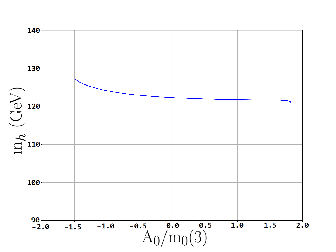
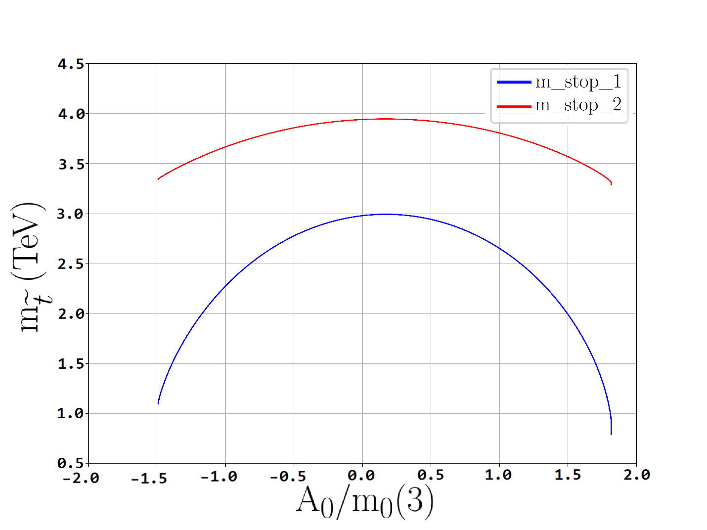
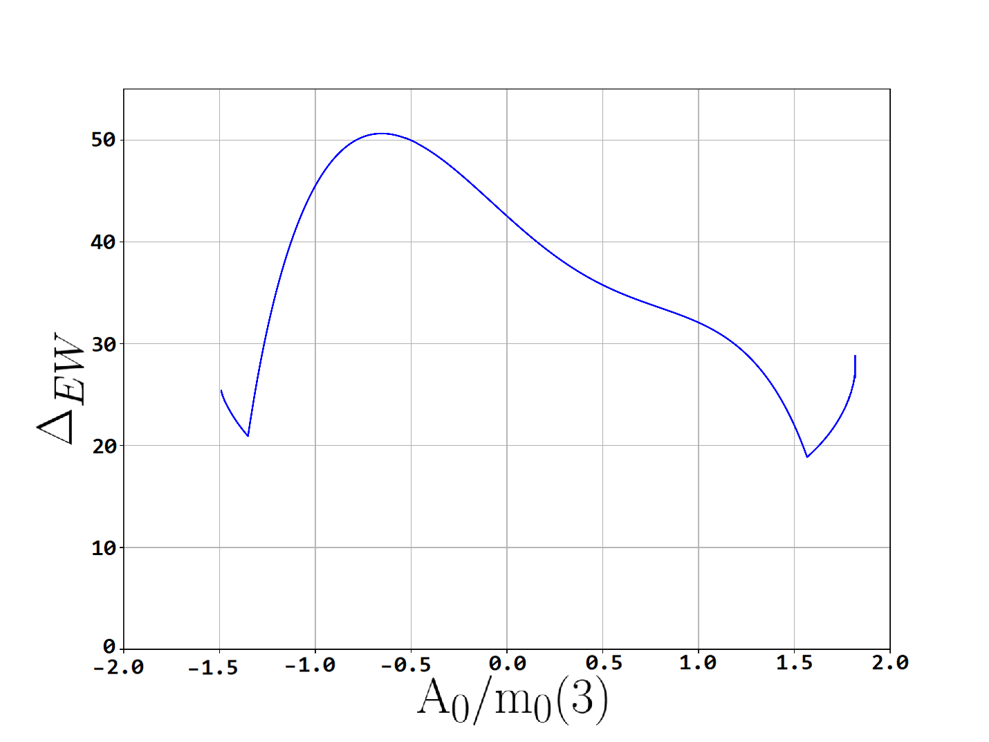
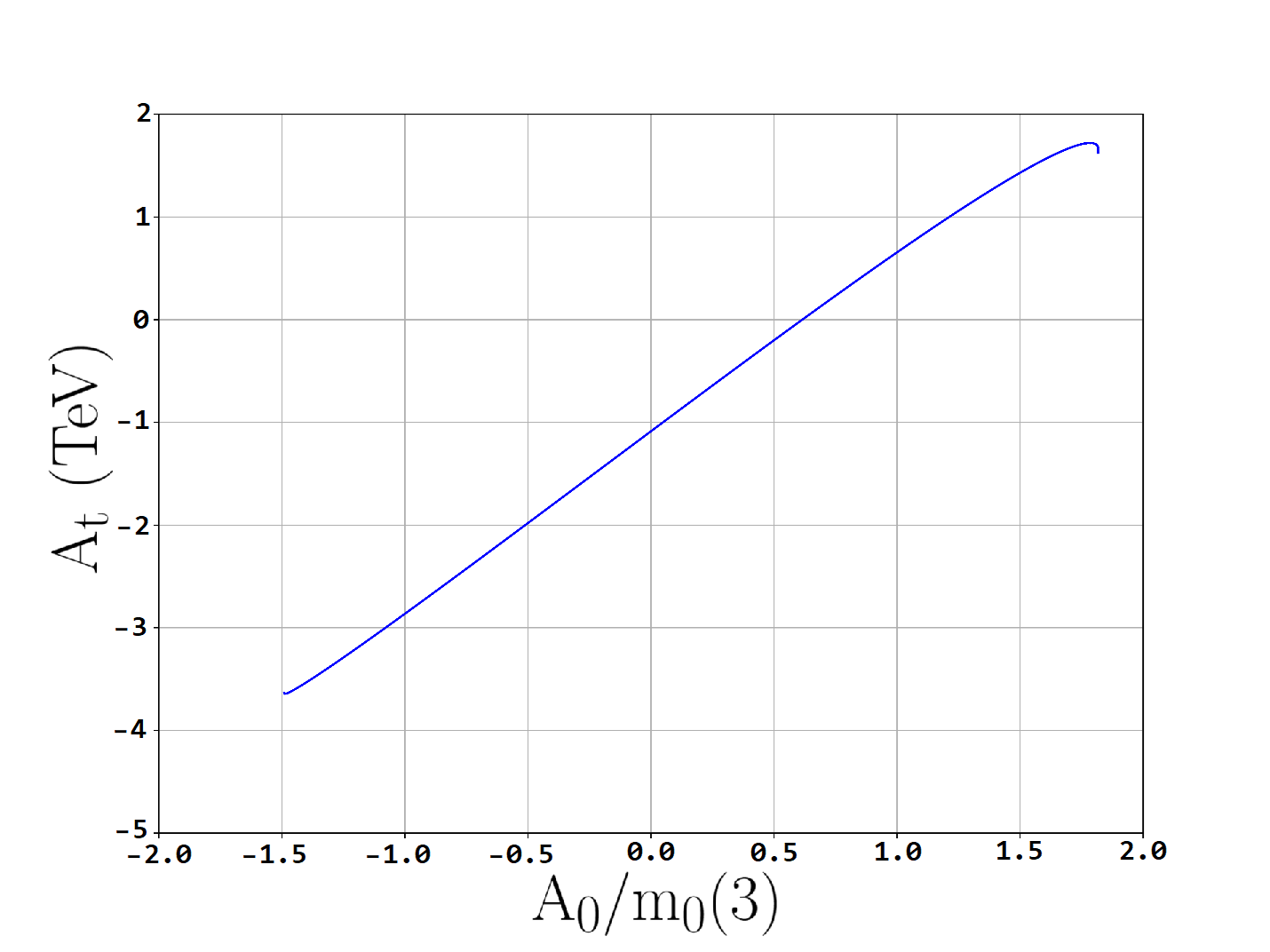
Figure 2: Values of a) $m_{h}$, b) $m_{\tilde{t}_{1,2}}$, c) $\Delta_{EW}$ and d) $A_{t}(Q)$ vs. $A_{0}/m_{0}(3)$ for the NUHM3 model with $m_{0}(1,2)=10$ TeV, $m_{0}(3)=5$ TeV, $m_{1/2}=0.7$ TeV, $\tan\beta=10$ with $\mu=200$ GeV and $m_{A}=2$ TeV.

In Fig. 3, we show the third generation contributions to $\Delta_{EW}$ vs. $A_{0}/m_{0}(3)$ for the same parameters as in Fig. 2, but using SOFTSUSY. These can be compared with the same plot using Isasugra in Fig. 2 of Ref. [15]. Here, we see that the contributions from staus and sbottoms are generally rather small, and the top-squark contributions typically dominate. But for large $|A_{0}/m_{0}(3)|$, then cancellations in both $\Sigma_{u}^{u}(\tilde{t}_{1})$ and $\Sigma_{u}^{u}(\tilde{t}_{2})$ occur, and the stop contributions become comparable to those of the other third generation sparticles, giving reduced finetuning and greater naturalness.

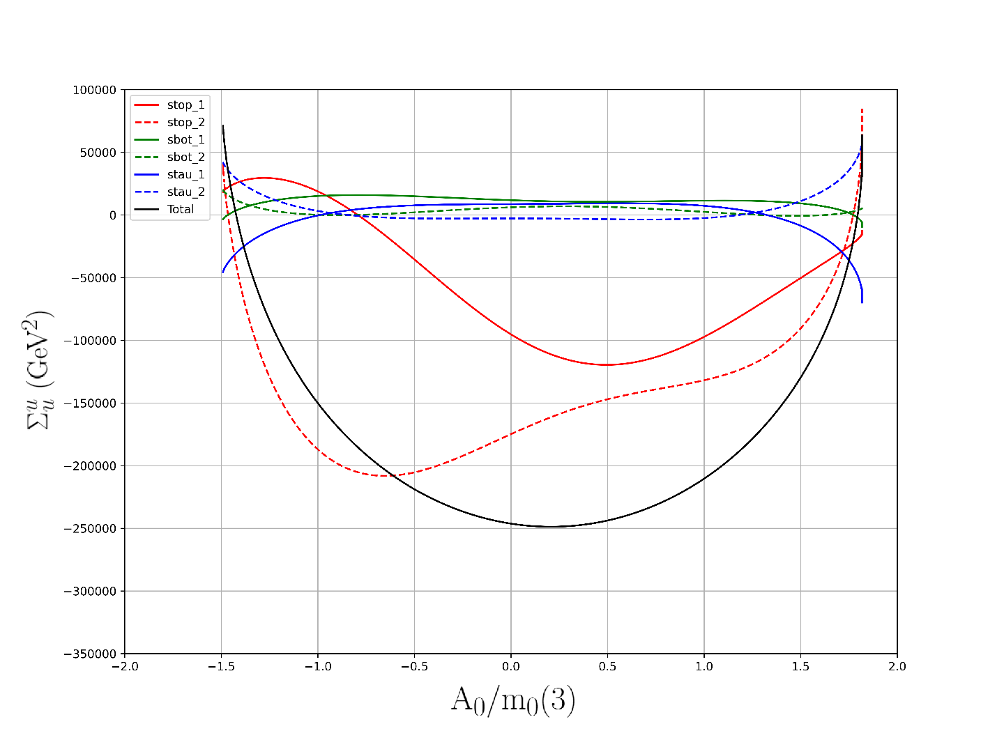
Figure 3: Third generation contributions to $\Delta_{EW}$ for the same model parameters as Fig. 2 vs. $A_{0}/m_{0}(3)$ in the $m_{0}$ vs. $m_{1/2}$ plane of the NUHM2 model with $\mu=200$, $\tan\beta=10$, $A_{0}=-1.6m_{0}$ and $m_{A}=2$ TeV.

3.1 Natural regions of $m_{0}$ vs. $m_{1/2}$ plane

In Fig. 4, we show the $m_{0}$ vs. $m_{1/2}$ parameter plane for the NUHM2 model with $A_{0}=-1.6m_{0}$, $\mu=200$ GeV and $m_{A}=2$ TeV. The plot is generated using SOFTSUSY but can be compared with similar results from Isasugra in Fig. 8b of Ref. [52]. From the plot, we see the lower-left corner is actually excluded due to charge-or-color-breaking (CCB) vacua which occur for too large $A_{0}$ values. Both SOFTSUSY and Isasugra generate CCB regions there. We also show contours of Higgs mass $m_{h}=123$ and $127$ GeV. These are qualitatively similar to the Isasugra results but shifted to the right by a couple hundred GeV in $m_{0}$. Thus, much of the parameter space allows for the measured Higgs mass $m_{h}\sim 125$ GeV. We also show naturalness contours for $\Delta_{EW}=15$ and 30. These can also be compared against the LHC Run 2 gluino mass limit $m_{\tilde{g}}\gtrsim 2.25$ TeV as shown by the light blue contour. The important point is that both SOFTSUSY and Isasugra agree that the bulk of this parameter space plane is EW natural, in accord with LHC gluino mass limits, and in accord with the measured Higgs mass. This is in contrast to older naturalness measures which required much lower gluino masses[1, 2, 3, 4] and also Higgs boson masses[53].

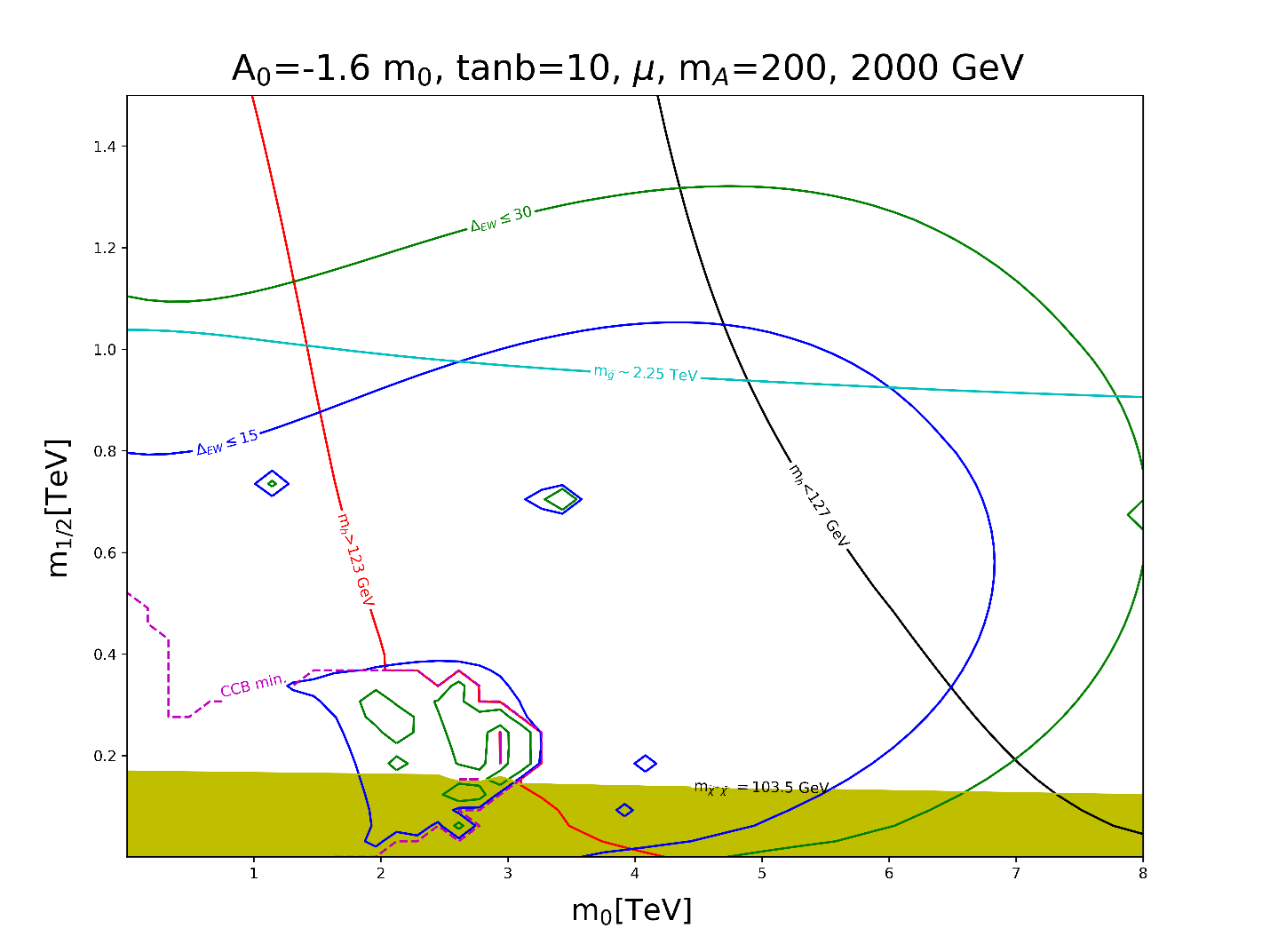
Figure 4: Contours of naturalness measure $\Delta_{EW}$ and $m_{h}$ in the $m_{0}$ vs. $m_{1/2}$ plane of the NUHM2 model with $\mu=200$, $\tan\beta=10$, $A_{0}=-1.6m_{0}$ and $m_{A}=2$ TeV.

4 String landscape distributions from SOFTSUSY

In this section, we wish to compare SUSY landscape predictions using a spectrum calculator other than Isasugra. Here, we choose SOFTSUSY. The assumption is that the MSSM is the low energy EFT in a fertile patch of landscape vacua, but with different sets of soft SUSY breaking terms in each pocket universe, and hence a different value for the weak scale $m_{weak}^{PU}\neq m_{weak}^{OU}$ in each pocket universe (here, $OU=$ our universe). Following Douglas[39], Susskind[40] and Arkani-Hamed, Dimopoulos and Kachru[41], we will assume the soft terms scan in the landscape as a power-law: $m_{soft}^{n}$ where $n=2n_{F}+n_{D}-1$ with $n_{F}$ the number of $F$ breaking fields and $n_{D}$ the number of $D$ breaking fields. Here, we assume $n=1$ corresponding to SUSY breaking by a single $F$ term, where $F$ is distributed as a random complex number. As in Ref. [54], we expect each soft term in the NUHM3 model to scan independently.

We perform the linear soft term scan over NUHM3 space as follows:

• $m_{0}(1,2):\ 0.1-60$ TeV,

• $m_{0}(3):\ 0.1-20$ TeV,

• $m_{1/2}:\ 0.5-10$ TeV,

• $A_{0}:\ -50\ -\ 0$ TeV,

• $m_{A}:\ 0.3-10$ TeV

with $\mu=200$ GeV and $\tan\beta$ scanned uniformly between $3-60$. The goal is to set upper limits on scan parameters that are beyond the upper limits that will result from imposing the anthropic conditions. We also require appropriate EWSB and so veto vacua with CCB minima or with no EWSB. We also require the Agrawal condition on the magnitude of the weak scale[43]:

• $m_{Z}^{PU}<4m_{Z}^{OU}$

which corresponds to $\Delta_{EW}<30$. Thus, the following results generated using SOFTSUSY can be compared to comparable results in Ref. [55] using Isasugra.

The resultant distribution in input parameters from the SOFTSUSY scan is shown in Fig. 5. In frame a), we see the distribution in first/second generation GUT scale soft masses peaks around 20 TeV and spans $\sim 5-40$ TeV. While first/second generation scalars contribute to the weak scale via Yukawa suppressed terms, they also contribute via EW $D$-term contributions (which largely cancel due to cancellation of EW quantum numbers) and via two-loop RG terms which, when large, drive third generation scalars to tachyonic values[23]. The last of these effectively sets the upper bound, allowing for $m_{0}(1,2)$ as high as $40-50$ TeV. This provides a mixed decoupling/quasi-degeneracy solution to the SUSY flavor and CP problems[24] since the upper bound is flavor independent. In frame b), the third generation soft masses are bounded by much lower values: $m_{0}(3)\sim 1-10$ TeV with a peak around 5 TeV. Here, the upper bound comes from requiring not-too-large values of $\Sigma_{u}^{u}(\tilde{t}_{1,2})$ values. In frame c), we see the distribution in $m_{1/2}$, which ranges form $0.5-3$ TeV. The upper bound is set because if $m_{1/2}$ is too large, it drives the stop soft terms to large values and again $\Sigma_{u}^{u}(\tilde{t}_{1,2})$ gets too big. In frame d), we plot the distribution in $-A_{0}$. There is hardly any probability around $A_{0}\sim 0$ so we expect large mixing in the stop sector, which ends up driving $m_{h}$ to large values. But $A_{0}$ cannot become too large (negative) lest it pushes the top squark soft terms to tachyonic values via RG running.

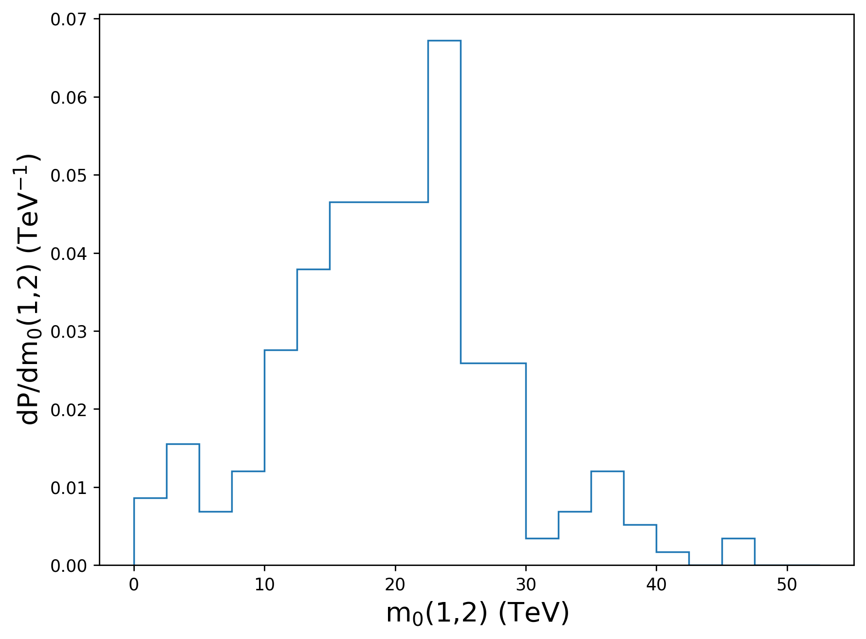
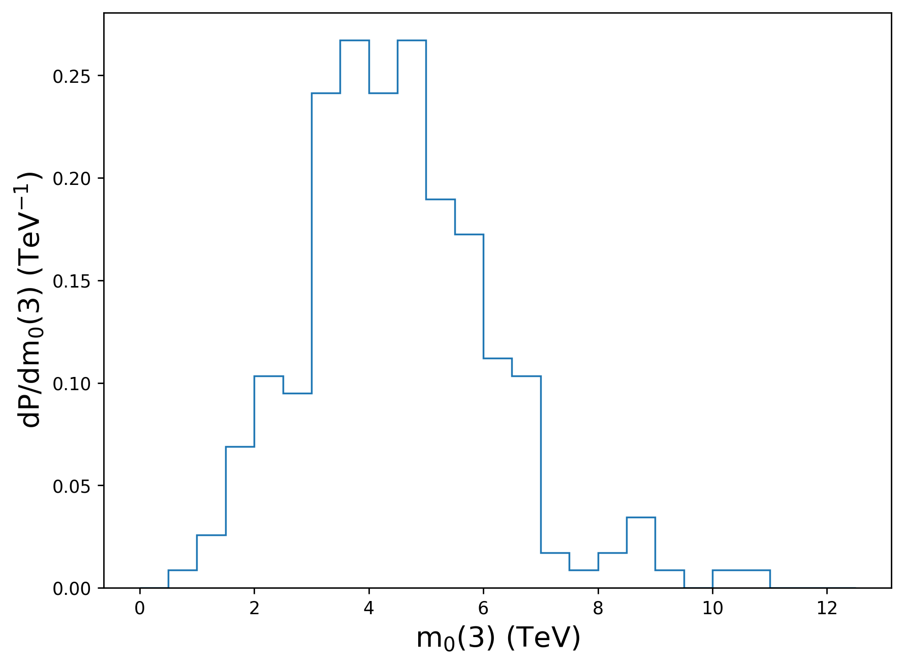
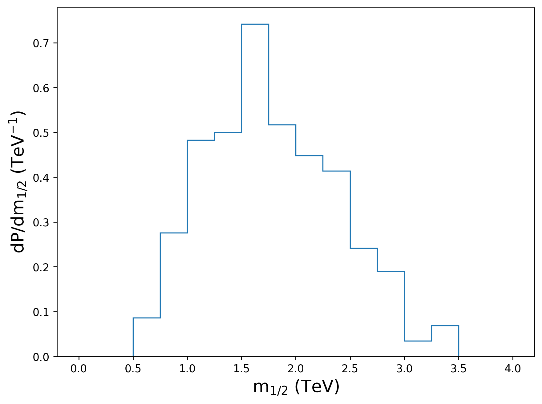
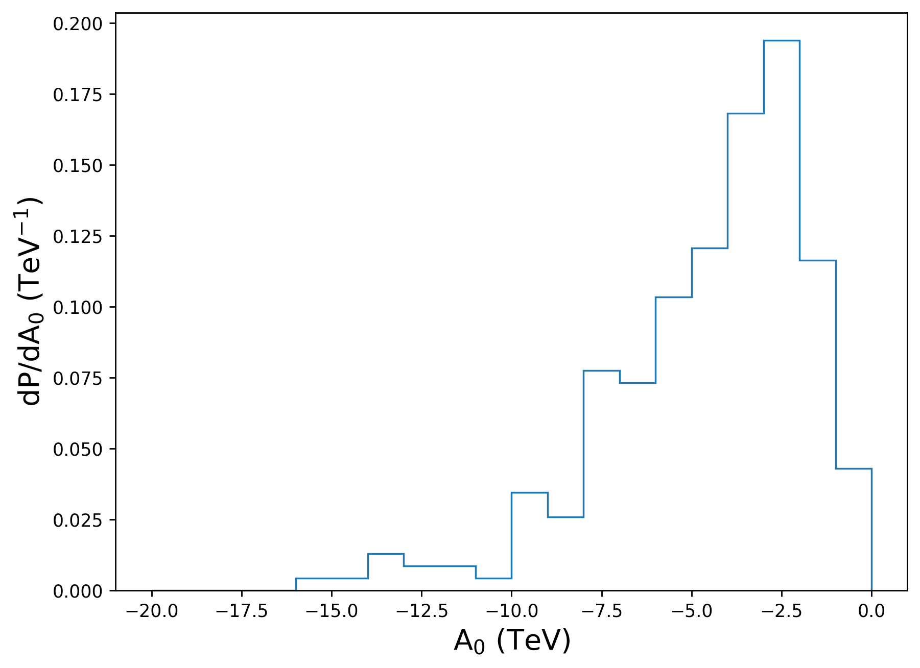
Figure 5: Distribution of soft SUSY breaking terms in subset of landscape vacua with the NUHM3 model as low energy EFT and an $n=1$ statistical draw. We show distributions in a) $m_{0}(1,2)$, b) $m_{0}(3)$, c) $m_{1/2}$ and d) $A_{0}$.

In Fig. 6, we show $n=1$ landscape scan probability distributions from the EW sector. In frame a), we show the distribution in light Higgs mass $m_{h}$. Using SOFTSUSY, the distribution rises to a peak $m_{h}\sim 128$ GeV, which is several GeV higher than the result from Isasugra. This is consistent with SOFTSUSY generating $m_{h}$ typically a couple GeV higher than Isasugra. In frame b), we see the distribution in $m_{A}$ which runs from $1-9$ TeV with a peak around 4 TeV. Thus, we expect a decoupled SUSY Higgs sector with the couplings of $h$ being very close to their SM values. In frame c), the distribution in $\tan\beta$ peaks around $10-20$. The upper bound is set because if $\tan\beta$ gets too big, then the $\Sigma_{u}^{u}(\tilde{b}_{1,2})$ terms become large (large $b$ and $\tau$ Yukawa couplings) and the model is more likely to generate a large $m_{weak}^{PU}$. In frame d), we show the $\tilde{\chi}_{2}^{0}-\tilde{\chi}_{1}^{0}$ mass difference which is important for LHC higgsino-pair searches[27]. In this case, the landscape predicts $m_{\tilde{\chi}_{2}^{0}}-m_{\tilde{\chi}_{1}^{0}}\sim 5-15$ GeV.

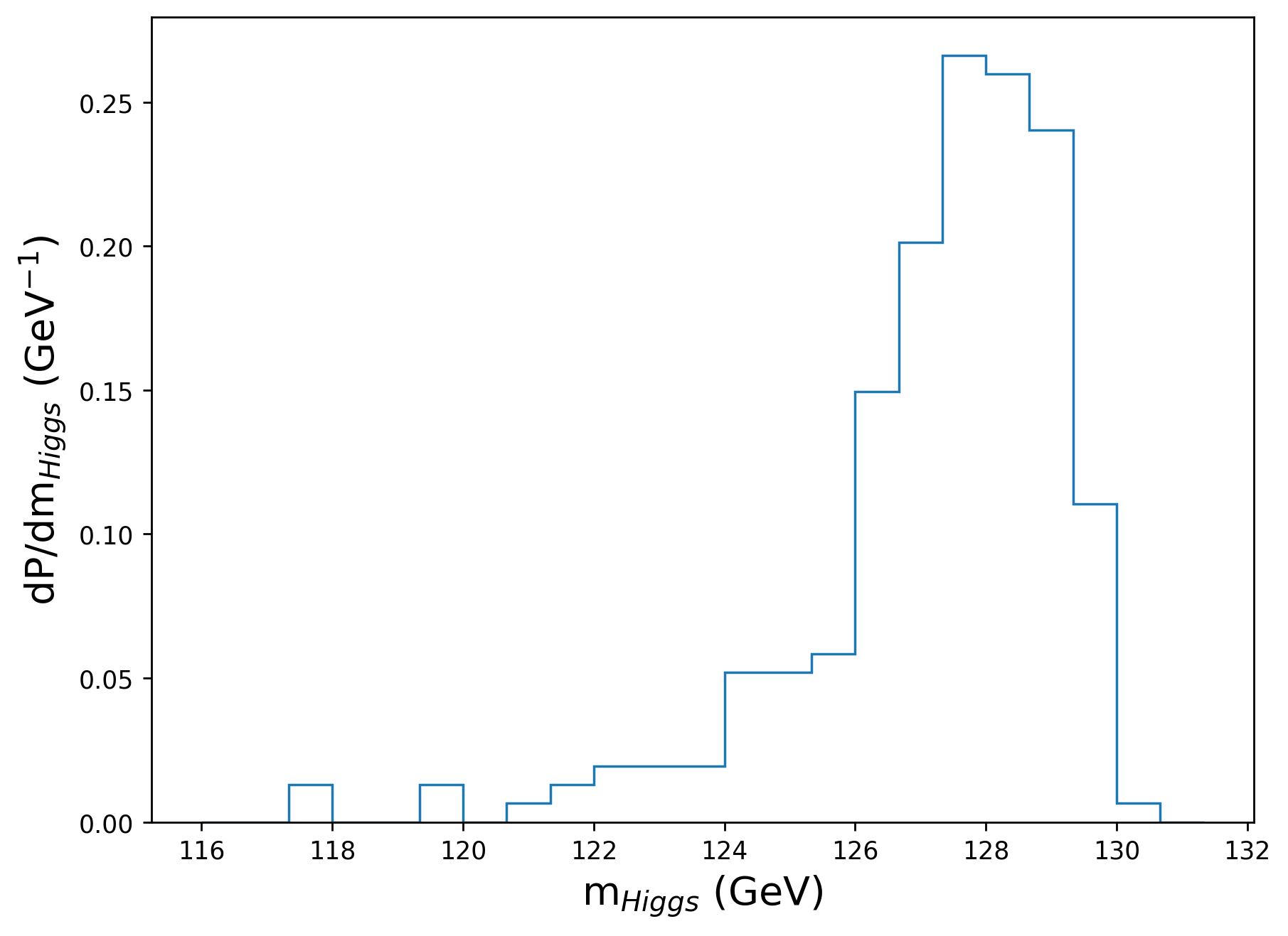
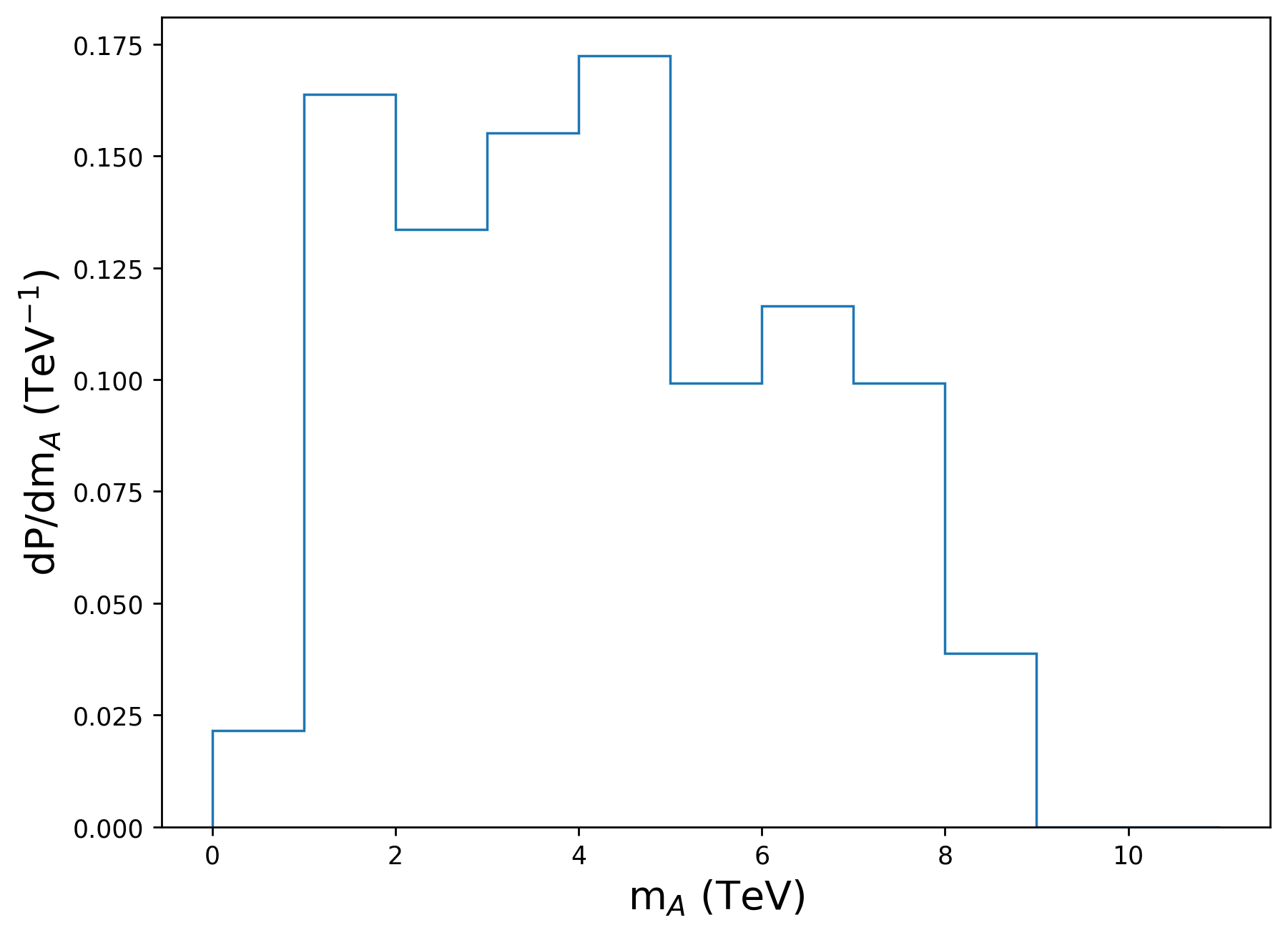
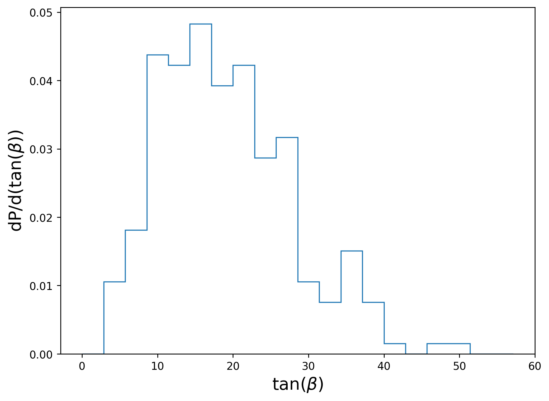
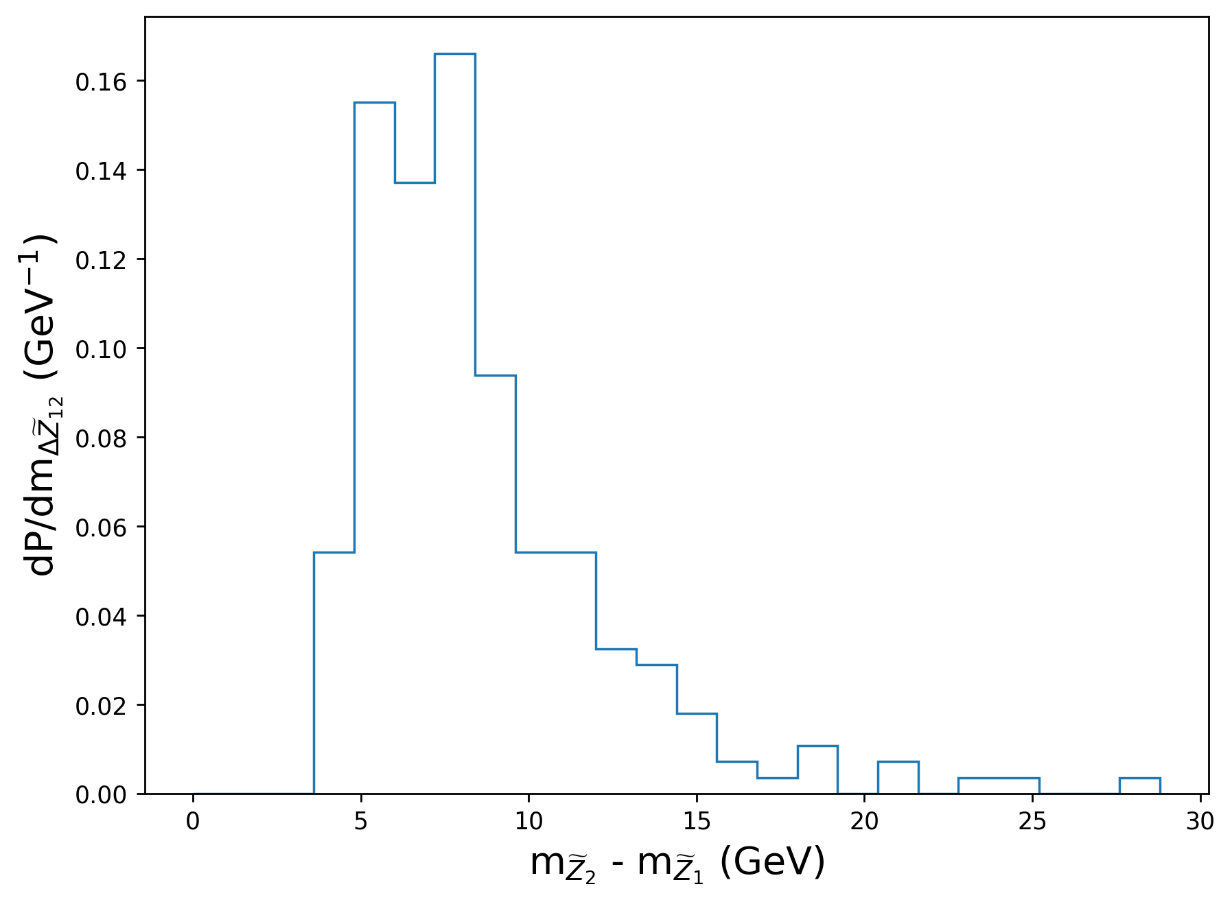
Figure 6: Distribution of Higgs and EWino sector from a subset of landscape vacua with NUHM3 model as low energy EFT and an $n=1$ statistical draw. We show distributions in a) $m_{h}$, b) $m_{A}$, c) $\tan\beta$ and d) $m_{\tilde{\chi}_{2}^{0}}-m_{\tilde{\chi}_{1}^{0}}$.

In Fig. 7, we show $n=1$ landscape distributions for strongly interacting SUSY particles using SOFTSUSY. In frame a), we see the gluino mass $m_{\tilde{g}}\sim 2-7$ TeV. The LHC13 limit of $m_{\tilde{g}}\gtrsim 2.25$ TeV just excludes the lower edge of the expected values. Thus, from the landscape point of view, it is no surprise that LHC has so far failed to detect gluinos. In frame b), we show the distribution in left up-squark mass (which is indicative of both first and second generation sfermion masses). The distribution ranges from $m_{\tilde{u}_{L}}\sim 10-40$ TeV, so these sparticles are likely far beyond LHC reach. In frame c), we show the distribution in light top-squark mass. Here we find $m_{\tilde{t}_{1}}\sim 1-2$ TeV, so again it may come as no surprise that LHC has so far not discovered evidence of top-squark pair production. The heavier top squark distribution $m_{\tilde{t}_{2}}$ is shown in frame d). Here we see it ranges between $2-5$ TeV. All these results are in qualitative agreement with previous results generated using Isasugra[55].

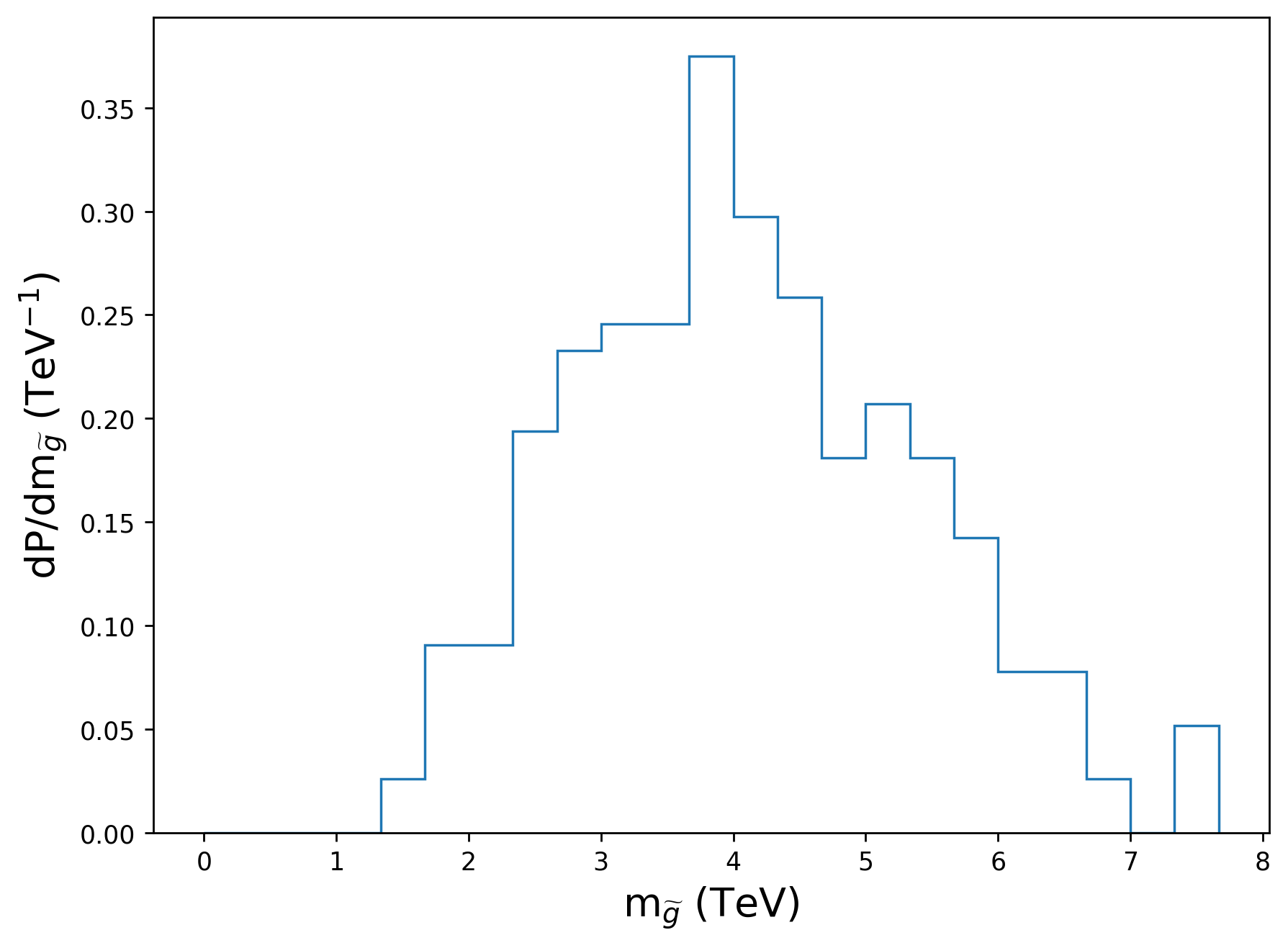
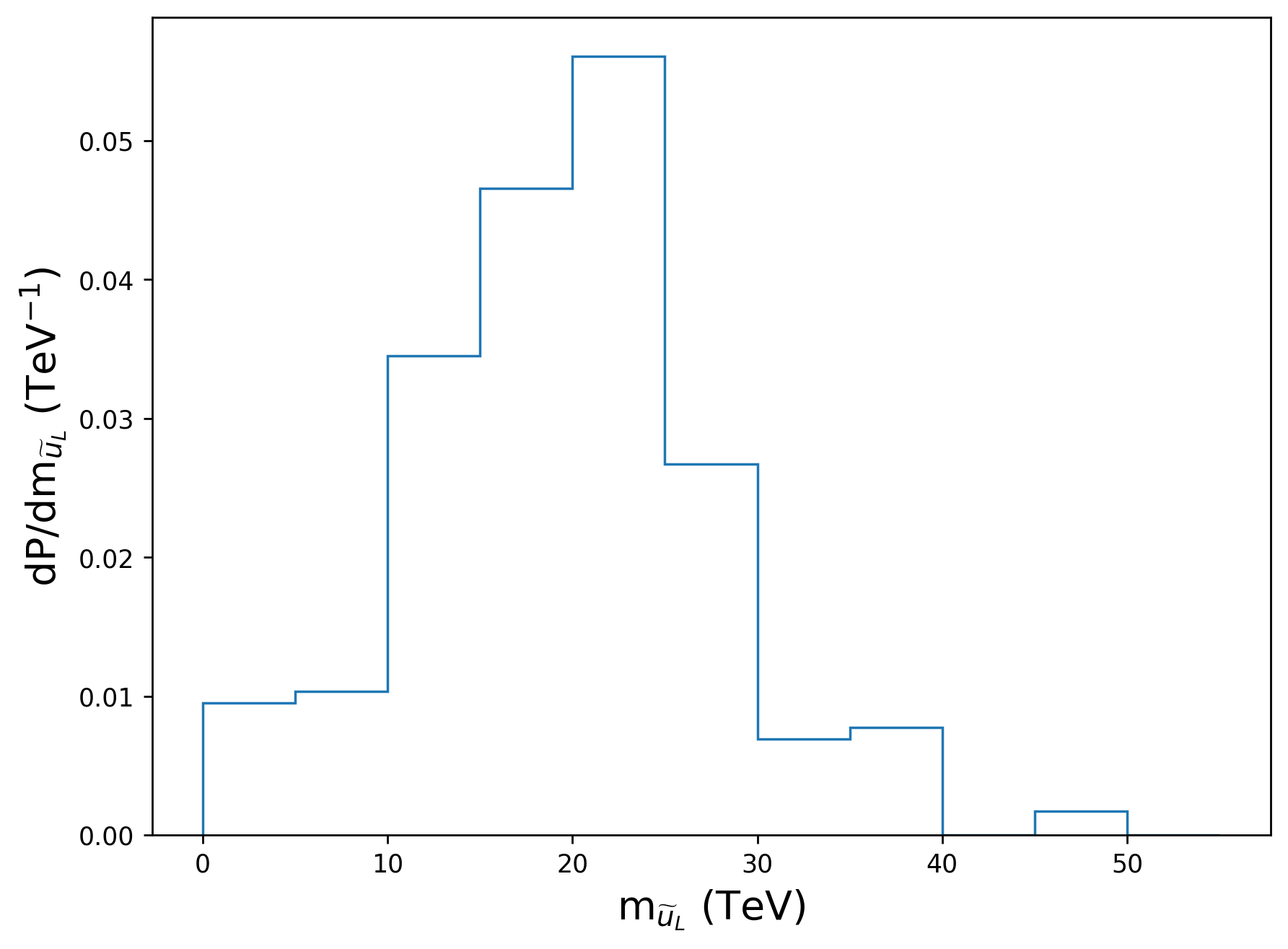
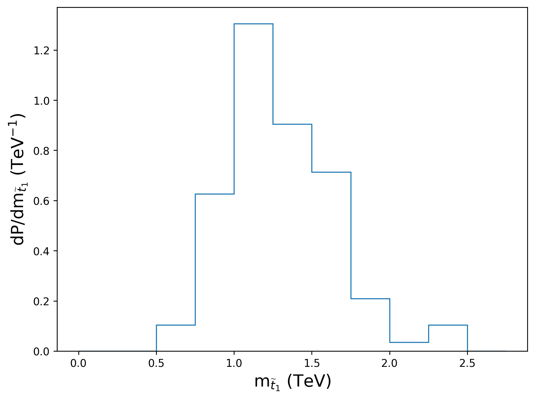
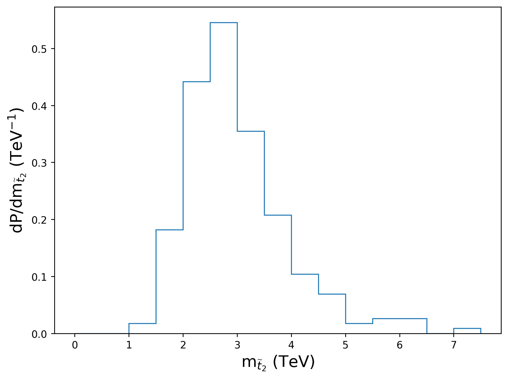
Figure 7: Distribution of strongly interacting sector masses from a subset of landscape vacua with NUHM3 model as low energy EFT and an $n=1$ statistical draw. We show distributions in a) $m_{\tilde{g}}$, b) $m_{\tilde{u}_{L}}$, c) $m_{\tilde{t}_{1}}$ and d) $m_{\tilde{t}_{2}}$.

5 Conclusions

We have created a publicly available computer code DEW4SLHA which computes the electroweak finetuning measure $\Delta_{EW}$ from any SUSY/Higgs spectrum generator which produces the standard SUSY Les Houches Accord output file. The code then allows us to compare naturalness and landscape predictions from various spectra codes against each other.

We have used the DEW4SLHA code in Sec. 3 to compare natural SUSY spectra from Isasugra, SOFTSUSY, SUSPECT and SPHENO. The outputs for a natural SUSY benchmark point are generally in good agreement although SOFTSUSY and SUSPECT gives values of $m_{h}$ a couple GeV higher than Isasugra or SPHENO. We also computed the top 44 contributions to $\Delta_{EW}$ which are typically in agreement although SPHENO generates slightly more stop mixing than the other codes. The SOFTSUSY code was used to display cancellations in $\Sigma_{u}^{u}(\tilde{t}_{1,2})$ that lead to increased naturalness for large stop mixing (which also lifts the value of $m_{h}\sim 125$ GeV).

We also used SOFTSUSY to corroborate predictions for sparticle and Higgs boson masses from the string landscape where a draw to large soft terms along with an anthropic requirement on the weak scale $m_{weak}^{PU}<4m_{weak}^{OU}$ leads to statistical predictions from compactified string models with the MSSM as the low energy EFT. SOFTSUSY generates a Higgs mass peak $m_{h}\sim 127-128$ GeV, slightly higher than Isasugra. SOFTSUSY also generates sparticle mass spectra typically beyond LHC13 reach, confirming earlier Isasugra results.

Appendix A Appendix of corrections

Starting with the effective potential, we have to one-loop order

$$V_{\text{Higgs}} =V_{\text{tree}}+\Delta V$$ (A.1)

$$V_{\text{tree}} =\left(\left\lvert\mu\right\rvert^{2}+m_{H_{u}}^{2}\right)\left\lvert H_{u}^{0}\right\rvert^{2}+\left(\left\lvert\mu\right\rvert^{2}+m_{H_{d}}^{2}\right)\left\lvert H_{d}^{0}\right\rvert^{2}-\left(bH_{u}^{0}H_{d}^{0}+\text{c.c.}\right)+\frac{\left(g^{2}+g^{\prime 2}\right)}{8}\left(\left\lvert H_{u}^{0}\right\rvert^{2}-\left\lvert H_{d}^{0}\right\rvert^{2}\right)^{2}$$ (A.2)

where $b\equiv B\mu$.

In the $\overline{\text{DR}}^{\prime}$ scheme, to remove the dependence of the 1-loop effective potential on $m_{\epsilon}^{2}$, we can write[56]

$$\Delta V =\frac{1}{16\pi^{2}}V^{(1)}_{\overline{\text{DR}}^{\prime}}$$ (A.3)

where

$$V^{(1)}_{\overline{\text{DR}}^{\prime}}=\sum\limits_{n}(-1)^{2s_{n}}\left(2s_{n}+1\right)h\left(m_{n}^{2}\right)\equiv\text{STr}(h(m_{n}^{2})),$$

$$h(x)=\frac{x^{2}}{4}\left[\overline{\ln}(x)-\frac{3}{2}\right]$$

and

$$\overline{\ln}(x)\equiv\ln\left(\frac{x}{Q^{2}}\right)$$

with $Q$ being the renormalization scale. One must also be careful to account for color multiplicity and charge multiplicity factors, where

$$n_{\widetilde{f}}=\begin{cases}1,&\widetilde{f}=\text{color neutral sparticle}\\ 3,&\widetilde{f}=\text{squark}\\ \end{cases}$$

represents the number of colors of $\widetilde{f}$ and

$$n_{\text{charge}}=\begin{cases}1,&\widetilde{f}\text{ is uncharged}\\ 2,&\widetilde{f}\text{ is charged}\\ \end{cases}.$$

For notation purposes, we may write

$$v_{u}=\left\langle H_{u}^{0}\right\rangle\ \ \ {\rm and}\ \ \ v_{d}=\left\langle H_{d}^{0}\right\rangle$$

such that

$$v_{u}^{2}+v_{d}^{2}=v^{2}=\frac{2m_{Z}^{2}}{g^{2}+g^{\prime 2}}\approx(174\text{ GeV})^{2}.$$

Then, defining the parameter $\beta$ through

$$\tan(\beta)\equiv\frac{v_{u}}{v_{d}}$$

one may write

$$v_{u}=v\sin(\beta)\ \ \ {\rm and}\ \ \ v_{d}=v\cos(\beta).$$

Therefore, the minimization conditions are:

$$m_{H_{u}}^{2}+\Sigma_{u}^{u}+\left\lvert\mu\right\rvert^{2}-b\cot(\beta)-\frac{m_{Z}^{2}}{2}\cos(2\beta) =0$$ (A.4)

and

$$m_{H_{d}}^{2}+\Sigma_{d}^{d}+\left\lvert\mu\right\rvert^{2}-b\tan(\beta)+\frac{m_{Z}^{2}}{2}\cos(2\beta) =0$$ (A.5)

where we treat $v_{u,d}$ as real variables in the differentiation such that the derivatives of $\Delta V(v_{u},v_{d})$ can be written as

$$\Sigma_{u}^{u} =\frac{\partial\Delta V\left(v_{u},v_{d}\right)}{\partial v_{u}^{2}}$$ (A.6)

$$=\frac{\partial\Delta V}{\partial v_{u}}\underbrace{\frac{\partial v_{u}}{\partial v_{u}^{2}}}_{\frac{1}{2v_{u}}}+\frac{\partial\Delta V}{\partial v_{d}}\underbrace{\frac{\partial v_{d}}{\partial v_{u}^{2}}}_{0}$$

$$=\frac{1}{2v_{u}}\frac{\partial\Delta V}{\partial v_{u}},$$

$$\Sigma_{d}^{d} =\frac{\partial\Delta V\left(v_{u},v_{d}\right)}{\partial v_{d}^{2}}$$ (A.7)

$$=\frac{\partial\Delta V}{\partial v_{u}}\underbrace{\frac{\partial v_{u}}{\partial v_{d}^{2}}}_{0}+\frac{\partial\Delta V}{\partial v_{d}}\underbrace{\frac{\partial v_{d}}{\partial v_{u}^{2}}}_{\frac{1}{2v_{d}}}$$

$$=\frac{1}{2v_{d}}\frac{\partial\Delta V}{\partial v_{d}},$$

$$\Sigma_{u}^{d} =\frac{\partial\left(\Delta V\right)}{\partial(v_{u}v_{d}+c.c.)},$$ (A.8)

with

$$\Sigma_{u}^{d} =\Sigma_{d}^{u}.$$ (A.9)

With these notes in mind, we can write the minimization conditions as

$$m_{Z}^{2} =\frac{\left\lvert m_{H_{d}}^{2}+\Sigma_{d}^{d}-m_{H_{u}}^{2}-\Sigma_{u}^{u}\right\rvert}{\underbrace{\sqrt{1-\sin^{2}(2\beta)}}_{\cos(2\beta)}}-m_{H_{u}}^{2}-\Sigma_{u}^{u}-m_{H_{d}}^{2}-\Sigma_{d}^{d}-2\left\lvert\mu\right\rvert^{2}$$ (A.10)

and

$$\sin(2\beta) =\frac{2b}{m^{2}_{H_{u}}+\Sigma_{u}^{u}+m_{H_{d}}^{2}+\Sigma_{d}^{d}+2\left\lvert\mu\right\rvert^{2}}$$ (A.11)

or equivalently

$$b=\left[\left(m_{H_{u}}^{2}+\Sigma_{u}^{u}+\left\lvert\mu\right\rvert^{2}\right)+\left(m_{H_{d}}^{2}+\Sigma_{d}^{d}+\left\lvert\mu\right\rvert^{2}\right)\right]\sin(\beta)\cos(\beta).$$

The $\Sigma$ contributions are, explicitly,

$$\Sigma_{u}^{u} =\sum\limits_{n}\frac{(-1)^{2s_{n}}}{32\pi^{2}}\left(2s_{n}+1\right)m_{n}^{2}\left(\frac{\partial m_{n}^{2}}{\partial v_{u}^{2}}\right)\left(\overline{\ln}\left(m_{n}^{2}\right)-1\right),$$ (A.12)

$$\Sigma_{d}^{d} =\sum\limits_{n}\frac{(-1)^{2s_{n}}}{32\pi^{2}}\left(2s_{n}+1\right)m_{n}^{2}\left(\frac{\partial m_{n}^{2}}{\partial v_{d}^{2}}\right)\left(\overline{\ln}\left(m_{n}^{2}\right)-1\right),$$

$$\Sigma_{u}^{d} =\Sigma_{d}^{u}$$

$$=\sum\limits_{n}\frac{(-1)^{2s_{n}}}{64\pi^{2}}\left(2s_{n}+1\right)m_{n}^{2}\left(\frac{\partial m_{n}^{2}}{\partial\left(v_{u}v_{d}\right)}\right)\left(\overline{\ln}\left(m_{n}^{2}\right)-1\right),$$

with

$$F(m^{2}) =m^{2}\left[\overline{\ln}\left(m^{2}\right)-1\right].$$ (A.13)

The color and charge factors are accounted for as mentioned above, and each individual contribution is given below.

Squarks and sleptons

The stop squark squared mass matrix is given by

$$\textbf{m}_{\widetilde{t}}^{2} =\begin{bmatrix}m^{2}_{\widetilde{t}_{L}}+m_{t}^{2}+\Delta_{\widetilde{u}_{L}}&a^{*}_{t}v_{u}-\mu y_{t}v_{d}\\ a_{t}v_{u}-\mu^{*}y_{t}v_{d}&m^{2}_{\widetilde{t}_{R}}+m_{t}^{2}+\Delta_{\widetilde{u}_{R}}\\ \end{bmatrix}$$ (A.14)

where

$$\Delta_{\phi} =\left(T_{3\phi}-Q_{\phi}\sin^{2}(\theta_{W})\right)\left(\frac{g^{2}+g^{\prime 2}}{2}\right)(v_{d}^{2}-v_{u}^{2})$$ (A.15)

where $T_{3\phi}$ is the third component of the weak isospin of $\phi$, and $Q_{\phi}$ is the electrical charge of $\phi$. Hence,

$$\frac{\partial\Delta_{\phi}}{\partial v_{u}^{2}}=-(T_{3\phi}-Q_{\phi}\underbrace{\sin^{2}(\theta_{W})}_{x_{W}})\left(\frac{g^{2}+g^{\prime 2}}{2}\right)$$

and

$$\frac{\partial\Delta_{\phi}}{\partial v_{d}^{2}}=\left(T_{3\phi}-Q_{\phi}x_{W}\right)\left(\frac{g^{2}+g^{\prime 2}}{2}\right).$$

At tree-level, the following mass relations hold for the running masses:

$$m_{t} =y_{t}v_{u},$$ (A.16)

$$m_{b} =y_{b}v_{d},$$ (A.17)

$$m_{\tau} =y_{\tau}v_{d}.$$ (A.18)

The eigenvalues of Eq. (A.14) are

$$m^{2}_{\widetilde{t}_{1,2}} =\frac{1}{2}\Bigg{(}m^{2}_{\widetilde{t}_{L}}+2m_{t}^{2}+m^{2}_{\widetilde{t}_{R}}+\Delta_{\widetilde{u}_{L}}+\Delta_{\widetilde{u}_{R}}$$ (A.19)

$$\mp\sqrt{(m^{2}_{\widetilde{t}_{L}}-m^{2}_{\widetilde{t}_{R}}+\Delta_{\widetilde{u}_{L}}-\Delta_{\widetilde{u}_{R}})^{2}+4\left[|a_{t}|^{2}v_{u}^{2}-v_{d}v_{u}y_{t}\mu^{*}a_{t}^{*}+v_{d}v_{u}y_{t}\mu a_{t}+v_{d}v_{u}+|\mu|^{2}v_{d}^{2}y_{t}^{2}\right]}\Bigg{)}$$

where $m^{2}_{\widetilde{t}_{1}}<m^{2}_{\widetilde{t}_{2}}$.

Note that

$$g_{Z}^{2}\equiv\frac{g^{2}+\left(g^{\prime}\right)^{2}}{8}\ \ {\rm so\ that}\ \ \ m_{Z}^{2}\equiv 4v^{2}\cdot g_{Z}^{2}.$$

The trilinear couplings are written in “reduced” form, i.e.,

$$a_{i}\equiv A_{i}\cdot y_{i}$$

with $y_{i}$ the corresponding Yukawa coupling.

The radiative correction terms are then

$$\Sigma_{u}^{u}(\widetilde{t}_{1,2}) =\frac{3}{16\pi^{2}}F(m_{\widetilde{t}_{1,2}}^{2})\cdot\left[y_{t}^{2}-g_{Z}^{2}\mp\frac{a_{t}^{2}-2g_{Z}^{2}\cdot\Delta_{\widetilde{t}}}{m_{\widetilde{t}_{2}}^{2}-m_{\widetilde{t}_{1}}^{2}}\right]$$ (A.20)

with

$$\Delta_{\widetilde{t}}\equiv 2\left(\frac{1}{2}-\frac{4}{3}\sin^{2}(\theta_{W})\right)\cdot\left[\frac{m_{\widetilde{t}_{L}}^{2}-m_{\widetilde{t}_{R}}^{2}}{2}+\left(m_{Z}^{2}\cos(2\beta)\cdot\left[\frac{1}{4}-\frac{2}{3}\sin^{2}(\theta_{W})\right]\right)\right]$$

and

$$\Sigma_{d}^{d}(\widetilde{t}_{1,2}) =\frac{3}{16\pi^{2}}F(m_{\widetilde{t}_{1,2}^{2}})\left[g_{Z}^{2}\mp\frac{y_{t}^{2}\cdot\mu^{2}+2g_{Z}^{2}\cdot\Delta_{\widetilde{t}}}{m_{\widetilde{t}_{2}}^{2}-m_{\widetilde{t}_{1}}^{2}}\right]$$ (A.21)

where the minus (plus) sign corresponds to $\widetilde{t}_{1(2)}$.

Next, with the bottom squark mass matrix

$$\textbf{m}_{\widetilde{b}}^{2} =\begin{bmatrix}m^{2}_{\widetilde{b}_{L}}+\Delta_{\widetilde{d}_{L}}&a^{*}_{b}v_{d}-\mu y_{b}v_{u}\\ a_{b}v_{d}-\mu^{*}y_{b}v_{d}&m^{2}_{\widetilde{b}_{R}}+\Delta_{\widetilde{d}_{R}}\\ \end{bmatrix},$$ (A.22)

the eigenvalues are computed to be

$$\leavevmode\resizebox{422.77661pt}{}{$m^{2}_{\widetilde{b}_{1,2}}=\frac{1}{2}\left(m^{2}_{\widetilde{b}_{L}}+\Delta_{\widetilde{d}_{L}}+m^{2}_{\widetilde{b}_{R}}+\Delta_{\widetilde{d}_{R}}\mp\sqrt{(-m^{2}_{\widetilde{b}_{L}}-\Delta_{\widetilde{d}_{L}}+m^{2}_{\widetilde{b}_{R}}+\Delta_{\widetilde{d}_{R}})^{2}+4(a_{b}^{*}v_{d}-\mu v_{u}y_{t})(a_{b}v_{d}-\mu^{*}v_{u}y_{t})}\right).$}$$ (A.23)

Thus, the radiative correction terms are

$$\Sigma_{u}^{u}(\widetilde{b}_{1,2}) =\frac{3}{16\pi^{2}}F(m_{\widetilde{b}_{1,2}}^{2})\cdot\left[y_{b}^{2}-g_{Z}^{2}\mp\frac{a_{b}^{2}-2g_{Z}^{2}\cdot\Delta_{\widetilde{b}}}{m_{\widetilde{b}_{2}}^{2}-m_{\widetilde{b}_{1}}^{2}}\right]$$ (A.24)

with

$$\Delta_{\widetilde{b}}=2\left(\frac{1}{2}-\frac{2}{3}\sin^{2}(\theta_{W})\right)\cdot\left(\frac{m_{b_{L}}^{2}-m_{b_{R}}^{2}}{2}-m_{Z}^{2}\cos(2\beta)\cdot\left[\frac{1}{4}-\frac{1}{3}\sin^{2}(\theta_{W})\right]\right)$$

and

$$\Sigma_{d}^{d}(\widetilde{b}_{1,2}) =\frac{3}{16\pi^{2}}F(m_{\widetilde{b}_{1,2}}^{2})\cdot\left[g_{Z}^{2}\mp\frac{y_{b}^{2}\cdot\mu^{2}+2g_{Z}^{2}\cdot\Delta_{\widetilde{b}}}{m_{\widetilde{b}_{2}}^{2}-m_{\widetilde{b}_{1}}^{2}}\right].$$ (A.25)

Similarly, one can obtain the result for the staus by exchanging $b\rightarrow\tau$, $n_{\widetilde{\tau},\text{ col.}}\rightarrow 1$, and

$$\Delta_{\widetilde{\tau}}\equiv 2\left(\frac{1}{2}-2\sin^{2}(\theta_{W})\right)\cdot\left[\frac{m_{\widetilde{\tau}_{L}}^{2}-m_{\widetilde{\tau}_{R}}^{2}}{2}-\left(\frac{1}{4}-\sin^{2}(\theta_{W})\right)\right].$$

Sfermions

For a general sfermion $\widetilde{f}_{L,R}$ in the first or second generation, the masses can be parameterized based on the boundary conditions of the model. It can be shown that for these sfermions,

$$\frac{\partial m_{\widetilde{f}}^{2}}{\partial v_{u,d}^{2}}=\overbrace{\underbrace{\pm}_{v_{u}^{2}}}^{v_{d}^{2}}(T_{3\widetilde{f}}-Q_{\widetilde{f}}x_{W})\left(\frac{g^{2}+g^{\prime 2}}{2}\right)$$ (A.26)

which leads to the cancellation between first and second generation sfermion corrections, where the cancellation arises between $\Sigma_{u}^{u}(\widetilde{f})$ and $\Sigma_{d}^{d}(\widetilde{f})$. Indeed, one finds that for the squarks,

$$\Sigma^{u}_{u}(\widetilde{f}_{L,R}) =\frac{-3}{4\pi^{2}}(T_{3\widetilde{f}_{L,R}}-Q_{\widetilde{f}_{L,R}}x_{W})g_{Z}^{2}F(m_{\widetilde{f}_{L,R}}^{2})$$ (A.27)

and

$$\Sigma^{d}_{d}(\widetilde{f}_{L,R}) =\frac{+3}{4\pi^{2}}(T_{3\widetilde{f}_{L,R}}-Q_{\widetilde{f}_{L,R}}x_{W})g_{Z}^{2}F(m_{\widetilde{f}_{L,R}}^{2}).$$ (A.28)

For the sleptons in the 1st and 2nd generations, replace the color factor of $3$ in the numerator with $1$, and for the slepton sneutrinos, replace the color factor of $3\rightarrow 1$ and the charge factor from $2\rightarrow 1$.

Neutralinos

For the neutralinos, the unsquared mass matrix can be given by the following, where $c_{\beta}=\cos(\beta),s_{\beta}=\sin(\beta)$, and likewise for other angles:

$$\textbf{m}_{\widetilde{N}} =\begin{bmatrix}M_{1}&0&-c_{\beta}s_{W}m_{Z}&s_{\beta}s_{W}m_{Z}\\ 0&M_{2}&c_{\beta}c_{W}m_{Z}&-s_{\beta}c_{W}m_{Z}\\ -c_{\beta}s_{W}m_{Z}&c_{\beta}c_{W}m_{Z}&0&-\mu\\ s_{\beta}s_{W}m_{Z}&-s_{\beta}c_{W}m_{Z}&-\mu&0\\ \end{bmatrix}.$$ (A.29)

One could square this matrix and solve for the eigenvalues by brute force using the Ferrari method, and then differentiating the resultant squared mass eigenvalues. Instead, we use the method proposed by Ibrahim and Nath for taking the derivatives of eigenvalues[57]. Consider the characteristic polynomial of the squared neutralino mass matrix. The coefficients will each be functions of $v_{u},v_{d}$. As such, one may write in general form

$$F(\lambda) =\lambda^{4}+b_{\lambda}(v_{u},v_{d})\lambda^{3}+c_{\lambda}(v_{u},v_{d})\lambda^{2}+d_{\lambda}(v_{u},v_{d})\lambda+e_{\lambda}(v_{u},v_{d})$$ (A.30)

$$=0.$$

Then the eigenvalues have derivatives given by

$$\frac{\partial m^{2}_{\widetilde{N}_{i}}}{\partial v_{u,d}^{2}} =\frac{-D_{v_{u,d}^{2}}F}{D_{\lambda}F}\Bigg{\rvert}_{\lambda=m^{2}_{\widetilde{N}_{i}}},$$ (A.31)

which can be obtained by taking the derivative of Eq. (A.30), with $i=1,2,3,4$,

$$D_{\lambda}F \equiv\frac{dF}{d\lambda},$$ (A.32)

and

$$D_{v_{u,d}^{2}}F =\frac{\partial b_{\lambda}}{\partial v_{u,d}^{2}}\lambda^{3}+\frac{\partial c_{\lambda}}{\partial v_{u,d}^{2}}\lambda^{2}+\frac{\partial d_{\lambda}}{\partial v_{u,d}^{2}}\lambda+\frac{\partial e_{\lambda}}{\partial v_{u,d}^{2}}/$$ (A.33)

From there, the explicit form of $\Sigma^{u,d}_{u,d}(\widetilde{N}_{i})$ for $i=1,2,3,4$ can be written, which will take the form

$$\Sigma^{u,d}_{u,d}(\widetilde{N}_{i}) =\frac{-1}{16\pi^{2}}\left[\frac{-D_{v_{u,d}^{2}}F}{D_{\lambda}F}\Bigg{\rvert}_{\lambda=m^{2}_{\widetilde{N}_{i}}}\right]F(m^{2}_{\widetilde{N}_{i}})/$$ (A.34)

Charginos

The chargino mass matrix is in $2\times 2$ block form on the off-diagonals, and can be squared to obtain the squared mass matrix,

$$\textbf{m}_{\widetilde{C}}^{2} =\begin{bmatrix}M_{2}^{2}+g^{2}v_{d}^{2}&g(M_{2}v_{u}+v_{d}\mu)&0&0\\ g(M_{2}v_{u}+\mu v_{d})&g^{2}v_{u}^{2}+\mu^{2}&0&0\\ 0&0&M_{2}^{2}+g^{2}v_{u}^{2}&g(M_{2}v_{d}+\mu v_{u})\\ 0&0&g(M_{2}v_{d}+\mu v_{u})&g^{2}v_{d}^{2}+\mu^{2}\\ \end{bmatrix}.$$ (A.35)

This has doubly degenerate eigenvalues

$$m^{2}_{\widetilde{C}_{1,2}} =\frac{1}{2}\left[|M_{2}|^{2}+|\mu|^{2}+g^{2}(v_{u}^{2}+v_{d}^{2})\mp\sqrt{\left[g^{2}(v_{u}+v_{d})^{2}+(M_{2}-\mu)^{2}\right]\left[g^{2}(v_{d}-v_{u})^{2}+(M_{2}+\mu)^{2}\right]}\right]$$ (A.36)

with $m^{2}_{\widetilde{C}_{1}}<m^{2}_{\widetilde{C}_{2}}$, leading to

$$\Sigma_{u}^{u}(\widetilde{C}_{1,2}) =\frac{-g^{2}}{16\pi^{2}}\left(1\mp\frac{(-2)\cdot m_{W}^{2}\cdot\cos(2\beta)+M_{2}^{2}+\mu^{2}}{m^{2}_{\widetilde{C}_{2}}-m^{2}_{\widetilde{C}_{1}}}\right)F(m^{2}_{\widetilde{C}_{1,2}})$$ (A.37)

and

$$\Sigma_{d}^{d}(\widetilde{C}_{1,2}) =\frac{-g^{2}}{16\pi^{2}}\left(1\mp\frac{2\cdot m_{W}^{2}\cdot\cos(2\beta)+M_{2}^{2}+\mu^{2}}{m^{2}_{\widetilde{C}_{2}}-m^{2}_{\widetilde{C}_{1}}}\right)F(m^{2}_{\widetilde{C}_{1,2}}).$$ (A.38)

with $m_{W}^{2}$ given below.

Weak bosons

Using the mass relations

$$m_{W}^{2} =\frac{g^{2}}{2}v^{2}\implies\ \frac{\partial m_{W}^{2}}{\partial v_{u,d}^{2}} =\frac{g^{2}}{2}$$ (A.39)

and

$$m_{Z}^{2} =\frac{(g^{2}+g^{\prime 2})}{2}(v^{2})\implies\ \frac{\partial m_{Z}^{2}}{\partial v_{u,d}^{2}} =\frac{g^{2}+g^{\prime 2}}{2}$$ (A.40)

such that the radiative corrections are

$$\Sigma^{u}_{u}(W^{\pm}) =\Sigma^{d}_{d}(W^{\pm})\ =\frac{3g^{2}}{32\pi^{2}}F(m_{W}^{2})$$ (A.41)

and

$$\Sigma^{u}_{u}(Z^{0}) =\Sigma^{d}_{d}(Z^{0})\ =\frac{3(g^{2}+g^{\prime 2})}{64\pi^{2}}F(m_{Z}^{2}).$$ (A.42)

Higgs bosons

For the Higgs bosons, we have the mass relations (with $m^{2}_{h_{0}}<m^{2}_{H_{0}}$)

$$m^{2}_{h_{0},H_{0}} =\frac{1}{2}\left(m_{A_{0}}^{2}+m_{Z}^{2}\mp\sqrt{(m_{A_{0}}^{2}-m_{Z}^{2})^{2}+4m_{Z}^{2}m_{A_{0}}^{2}\sin^{2}(2\beta)}\right)$$ (A.43)

and

$$m^{2}_{A_{0}} =\frac{2b}{\sin(2\beta)}\ =2|\mu|^{2}+m^{2}_{H_{u}}+m^{2}_{H_{d}}$$ (A.44)

Therefore,

$$\Sigma^{u}_{u}(h_{0},H_{0}) =\frac{g_{Z}^{2}}{16\pi^{2}}\left[1\mp\frac{m_{Z}^{2}+m_{A_{0}}^{2}\cdot\left(1+4\cos(2\beta)+2\cos^{2}(2\beta)\right)}{m^{2}_{H_{0}}-m^{2}_{h_{0}}}\right]F(m_{h_{0},H_{0}}^{2})$$ (A.45)

and

$$\Sigma^{d}_{d}(h_{0},H_{0}) =\frac{g_{Z}^{2}}{16\pi^{2}}\left[1\mp\frac{m_{Z}^{2}+m_{A_{0}}^{2}\cdot\left(1-4\cos(2\beta)+2\cos^{2}(2\beta)\right)}{m^{2}_{H_{0}}-m^{2}_{h_{0}}}\right]F(m_{h_{0},H_{0}}^{2}).$$ (A.46)

Then, for the charged Higgs, with the relation

$$m^{2}_{H^{\pm}} =m^{2}_{A_{0}}+m_{W}^{2}$$ (A.47)

one simply finds that

$$\Sigma^{u,d}_{u,d}(H^{\pm}) =\frac{g^{2}}{32\pi^{2}}F(m^{2}_{H^{\pm}}).$$ (A.48)

SM fermions

Finally, we can use the mass relations mentioned in Eqs. (16) - (18) to obtain the top, bottom, and $\tau$ contributions:

$$\Sigma^{u}_{u}(t) =\frac{-3y_{t}^{2}}{16\pi^{2}}F(m_{t}^{2}),$$ (A.49)

$$\Sigma^{d}_{d}(t) =0,$$ (A.50)

$$\Sigma^{u}_{u}(b) =0,$$ (A.51)

$$\Sigma^{d}_{d}(b) =\frac{-3y_{b}^{2}}{16\pi^{2}}F(m_{b}^{2}),$$ (A.52)

$$\Sigma^{u}_{u}(\tau) =0,$$ (A.53)

and

$$\Sigma^{d}_{d}(\tau) =\frac{-y_{\tau}^{2}}{16\pi^{2}}F(m_{\tau}^{2}).$$ (A.54)

We choose

$$Q=\sqrt{m_{\text{stop}_{1}}m_{\text{stop}_{2}}}$$ (A.55)

as the renormalization scale used in the function $F$.

From these terms, one can use the minimization conditions to define the naturalness measure $\Delta_{EW}$:

$$\Delta_{EW} \equiv\frac{2\max\left\lvert C_{i}\right\rvert}{m_{Z}^{2}}$$ (A.56)

where the $C_{i}$ terms are the individual contributions from the Higgs minimization condition ($i=H_{u},H_{d},\mu,\Sigma_{u}^{u},\Sigma_{d}^{d}$). Specifically, $C_{\mu}=\left\lvert\mu\right\rvert^{2}$,

$$C_{H_{u}}=\frac{-m_{H_{u}}^{2}\tan^{2}(\beta)}{\tan^{2}(\beta)-1}\ \ {\rm and}\ \ C_{H_{d}}=\frac{m_{H_{d}}^{2}}{\tan^{2}(\beta)-1},$$

and

$$C_{\Sigma_{u}^{u}}=\frac{-\Sigma_{u}^{u}\tan^{2}(\beta)}{\tan^{2}(\beta)-1}\ \ {\rm with}\ \ C_{\Sigma_{d}^{d}}=\frac{\Sigma_{d}^{d}}{\tan^{2}(\beta)-1}.$$

References

- [1] J. R. Ellis, K. Enqvist, D. V. Nanopoulos, F. Zwirner, Observables in Low-Energy Superstring Models, Mod. Phys. Lett. A 1 (1986) 57. doi:10.1142/S0217732386000105.
- [2] R. Barbieri, G. F. Giudice, Upper Bounds on Supersymmetric Particle Masses, Nucl. Phys. B 306 (1988) 63–76. doi:10.1016/0550-3213(88)90171-X.
- [3] S. Dimopoulos, G. F. Giudice, Naturalness constraints in supersymmetric theories with nonuniversal soft terms, Phys. Lett. B 357 (1995) 573–578. arXiv:hep-ph/9507282, doi:10.1016/0370-2693(95)00961-J.
- [4] G. W. Anderson, D. J. Castano, Naturalness and superpartner masses or when to give up on weak scale supersymmetry, Phys. Rev. D 52 (1995) 1693–1700. arXiv:hep-ph/9412322, doi:10.1103/PhysRevD.52.1693.
- [5] G. Aad, et al., Search for squarks and gluinos in final states with jets and missing transverse momentum using 139 fb-1 of =13 TeV collision data with the ATLAS detector, JHEP 02 (2021) 143. arXiv:2010.14293, doi:10.1007/JHEP02(2021)143.
- [6] A. M. Sirunyan, et al., Search for supersymmetry in proton-proton collisions at 13 TeV in final states with jets and missing transverse momentum, JHEP 10 (2019) 244. arXiv:1908.04722, doi:10.1007/JHEP10(2019)244.
- [7] R. Barbieri, A. Strumia, The ’LEP paradox’, in: 4th Rencontres du Vietnam: Physics at Extreme Energies (Particle Physics and Astrophysics), 2000. arXiv:hep-ph/0007265.
- [8] J. Lykken, M. Spiropulu, Supersymmetry and the Crisis in Physics, Sci. Am. 310N5 (2014) 36–39.
- [9] M. Dine, Naturalness Under Stress, Ann. Rev. Nucl. Part. Sci. 65 (2015) 43–62. arXiv:1501.01035, doi:10.1146/annurev-nucl-102014-022053.
- [10] N. Craig, The State of Supersymmetry after Run I of the LHC, in: Beyond the Standard Model after the first run of the LHC, 2013. arXiv:1309.0528.
- [11] H. Baer, X. Tata, Weak scale supersymmetry: From superfields to scattering events, Cambridge University Press, 2006.
- [12] H. Baer, V. Barger, D. Mickelson, How conventional measures overestimate electroweak fine-tuning in supersymmetric theory, Phys. Rev. D 88 (9) (2013) 095013. arXiv:1309.2984, doi:10.1103/PhysRevD.88.095013.
- [13] A. Mustafayev, X. Tata, Supersymmetry, Naturalness, and Light Higgsinos, Indian J. Phys. 88 (2014) 991–1004. arXiv:1404.1386, doi:10.1007/s12648-014-0504-8.
- [14] H. Baer, V. Barger, D. Mickelson, M. Padeffke-Kirkland, SUSY models under siege: LHC constraints and electroweak fine-tuning, Phys. Rev. D 89 (11) (2014) 115019. arXiv:1404.2277, doi:10.1103/PhysRevD.89.115019.
- [15] H. Baer, V. Barger, P. Huang, A. Mustafayev, X. Tata, Radiative natural SUSY with a 125 GeV Higgs boson, Phys. Rev. Lett. 109 (2012) 161802. arXiv:1207.3343, doi:10.1103/PhysRevLett.109.161802.
- [16] H. Baer, V. Barger, P. Huang, D. Mickelson, A. Mustafayev, X. Tata, Radiative natural supersymmetry: Reconciling electroweak fine-tuning and the Higgs boson mass, Phys. Rev. D 87 (11) (2013) 115028. arXiv:1212.2655, doi:10.1103/PhysRevD.87.115028.
- [17] H. Baer, V. Barger, M. Savoy, Upper bounds on sparticle masses from naturalness or how to disprove weak scale supersymmetry, Phys. Rev. D 93 (3) (2016) 035016. arXiv:1509.02929, doi:10.1103/PhysRevD.93.035016.
- [18] M. K. Gaillard, B. W. Lee, Rare Decay Modes of the K-Mesons in Gauge Theories, Phys. Rev. D 10 (1974) 897. doi:10.1103/PhysRevD.10.897.
- [19] S. P. Martin, A Supersymmetry primer, Adv. Ser. Direct. High Energy Phys. 18 (1998) 1–98. arXiv:hep-ph/9709356, doi:10.1142/9789812839657_0001.
- [20] A. Dedes, P. Slavich, Two loop corrections to radiative electroweak symmetry breaking in the MSSM, Nucl. Phys. B 657 (2003) 333–354. arXiv:hep-ph/0212132, doi:10.1016/S0550-3213(03)00173-1.
- [21] C. Brust, A. Katz, S. Lawrence, R. Sundrum, SUSY, the Third Generation and the LHC, JHEP 03 (2012) 103. arXiv:1110.6670, doi:10.1007/JHEP03(2012)103.
- [22] M. Papucci, J. T. Ruderman, A. Weiler, Natural SUSY Endures, JHEP 09 (2012) 035. arXiv:1110.6926, doi:10.1007/JHEP09(2012)035.
- [23] H. Baer, C. Balazs, P. Mercadante, X. Tata, Y. Wang, Viable supersymmetric models with an inverted scalar mass hierarchy at the GUT scale, Phys. Rev. D 63 (2001) 015011. arXiv:hep-ph/0008061, doi:10.1103/PhysRevD.63.015011.
- [24] H. Baer, V. Barger, D. Sengupta, Landscape solution to the SUSY flavor and CP problems, Phys. Rev. Res. 1 (3) (2019) 033179. arXiv:1910.00090, doi:10.1103/PhysRevResearch.1.033179.
- [25] H. Baer, V. Barger, S. Salam, D. Sengupta, K. Sinha, Status of weak scale supersymmetry after LHC Run 2 and ton-scale noble liquid WIMP searches, Eur. Phys. J. ST 229 (21) (2020) 3085–3141. arXiv:2002.03013, doi:10.1140/epjst/e2020-000020-x.
- [26] H. Baer, V. Barger, P. Huang, Hidden SUSY at the LHC: the light higgsino-world scenario and the role of a lepton collider, JHEP 11 (2011) 031. arXiv:1107.5581, doi:10.1007/JHEP11(2011)031.
- [27] H. Baer, A. Mustafayev, X. Tata, Monojet plus soft dilepton signal from light higgsino pair production at LHC14, Phys. Rev. D 90 (11) (2014) 115007. arXiv:1409.7058, doi:10.1103/PhysRevD.90.115007.
- [28] H. Baer, V. Barger, D. Sengupta, X. Tata, New angular (and other) cuts to improve the higgsino signal at the LHCarXiv:2109.14030.
- [29] H. Baer, A. Lessa, S. Rajagopalan, W. Sreethawong, Mixed axion/neutralino cold dark matter in supersymmetric models, JCAP 06 (2011) 031. arXiv:1103.5413, doi:10.1088/1475-7516/2011/06/031.
- [30] F. E. Paige, S. D. Protopopescu, H. Baer, X. Tata, ISAJET 7.69: A Monte Carlo event generator for pp, anti-p p, and e+e- reactionsarXiv:hep-ph/0312045.
- [31] H. Baer, C.-H. Chen, R. B. Munroe, F. E. Paige, X. Tata, Multichannel search for minimal supergravity at and colliders, Phys. Rev. D 51 (1995) 1046–1050. arXiv:hep-ph/9408265, doi:10.1103/PhysRevD.51.1046.
- [32] A. Djouadi, J.-L. Kneur, G. Moultaka, SuSpect: A Fortran code for the supersymmetric and Higgs particle spectrum in the MSSM, Comput. Phys. Commun. 176 (2007) 426–455. arXiv:hep-ph/0211331, doi:10.1016/j.cpc.2006.11.009.
- [33] B. C. Allanach, SOFTSUSY: a program for calculating supersymmetric spectra, Comput. Phys. Commun. 143 (2002) 305–331. arXiv:hep-ph/0104145, doi:10.1016/S0010-4655(01)00460-X.
- [34] W. Porod, SPheno, a program for calculating supersymmetric spectra, SUSY particle decays and SUSY particle production at e+ e- colliders, Comput. Phys. Commun. 153 (2003) 275–315. arXiv:hep-ph/0301101, doi:10.1016/S0010-4655(03)00222-4.
- [35] H. Bahl, T. Hahn, S. Heinemeyer, W. Hollik, S. Paßehr, H. Rzehak, G. Weiglein, Precision calculations in the MSSM Higgs-boson sector with FeynHiggs 2.14, Comput. Phys. Commun. 249 (2020) 107099. arXiv:1811.09073, doi:10.1016/j.cpc.2019.107099.
- [36] J. Pardo Vega, G. Villadoro, SusyHD: Higgs mass Determination in Supersymmetry, JHEP 07 (2015) 159. arXiv:1504.05200, doi:10.1007/JHEP07(2015)159.
- [37] P. Slavich, et al., Higgs-mass predictions in the MSSM and beyond, Eur. Phys. J. C 81 (5) (2021) 450. arXiv:2012.15629, doi:10.1140/epjc/s10052-021-09198-2.
- [38] P. Z. Skands, et al., SUSY Les Houches accord: Interfacing SUSY spectrum calculators, decay packages, and event generators, JHEP 07 (2004) 036. arXiv:hep-ph/0311123, doi:10.1088/1126-6708/2004/07/036.
- [39] M. R. Douglas, Statistical analysis of the supersymmetry breaking scalearXiv:hep-th/0405279.
- [40] L. Susskind, Supersymmetry breaking in the anthropic landscape, in: From Fields to Strings: Circumnavigating Theoretical Physics: A Conference in Tribute to Ian Kogan, 2004, pp. 1745–1749. arXiv:hep-th/0405189, doi:10.1142/9789812775344_0040.
- [41] N. Arkani-Hamed, S. Dimopoulos, S. Kachru, Predictive landscapes and new physics at a TeVarXiv:hep-th/0501082.
- [42] I. Broeckel, M. Cicoli, A. Maharana, K. Singh, K. Sinha, Moduli Stabilisation and the Statistics of SUSY Breaking in the Landscape, JHEP 10 (2020) 015. arXiv:2007.04327, doi:10.1007/JHEP09(2021)019.
- [43] V. Agrawal, S. M. Barr, J. F. Donoghue, D. Seckel, Viable range of the mass scale of the standard model, Phys. Rev. D 57 (1998) 5480–5492. arXiv:hep-ph/9707380, doi:10.1103/PhysRevD.57.5480.
- [44] V. Agrawal, S. M. Barr, J. F. Donoghue, D. Seckel, Anthropic considerations in multiple domain theories and the scale of electroweak symmetry breaking, Phys. Rev. Lett. 80 (1998) 1822–1825. arXiv:hep-ph/9801253, doi:10.1103/PhysRevLett.80.1822.
- [45] B. Allanach, S. Kraml, W. Porod, Comparison of SUSY mass spectrum calculations, in: 10th International Conference on Supersymmetry and Unification of Fundamental Interactions (SUSY02), 2002, pp. 904–910. arXiv:hep-ph/0207314.
- [46] G. Belanger, S. Kraml, A. Pukhov, Comparison of SUSY spectrum calculations and impact on the relic density constraints from WMAP, Phys. Rev. D 72 (2005) 015003. arXiv:hep-ph/0502079, doi:10.1103/PhysRevD.72.015003.
- [47] M. van Beekveld, W. Beenakker, S. Caron, R. Peeters, R. Ruiz de Austri, Supersymmetry with Dark Matter is still natural, Phys. Rev. D 96 (3) (2017) 035015. arXiv:1612.06333, doi:10.1103/PhysRevD.96.035015.
- [48] M. van Beekveld, S. Caron, R. Ruiz de Austri, The current status of fine-tuning in supersymmetry, JHEP 01 (2020) 147. arXiv:1906.10706, doi:10.1007/JHEP01(2020)147.
- [49] J. R. Ellis, T. Falk, K. A. Olive, Y. Santoso, Exploration of the MSSM with nonuniversal Higgs masses, Nucl. Phys. B 652 (2003) 259–347. arXiv:hep-ph/0210205, doi:10.1016/S0550-3213(02)01144-6.
- [50] H. Baer, A. Mustafayev, S. Profumo, A. Belyaev, X. Tata, Direct, indirect and collider detection of neutralino dark matter in SUSY models with non-universal Higgs masses, JHEP 07 (2005) 065. arXiv:hep-ph/0504001, doi:10.1088/1126-6708/2005/07/065.
- [51] D. M. Pierce, J. A. Bagger, K. T. Matchev, R.-j. Zhang, Precision corrections in the minimal supersymmetric standard model, Nucl. Phys. B 491 (1997) 3–67. arXiv:hep-ph/9606211, doi:10.1016/S0550-3213(96)00683-9.
- [52] H. Baer, V. Barger, S. Salam, Naturalness versus stringy naturalness (with implications for collider and dark matter searches, Phys. Rev. Research. 1 (2019) 023001. arXiv:1906.07741, doi:10.1103/PhysRevResearch.1.023001.
- [53] S. Cassel, D. M. Ghilencea, G. G. Ross, Testing SUSY, Phys. Lett. B 687 (2010) 214–218. arXiv:0911.1134, doi:10.1016/j.physletb.2010.03.032.
- [54] H. Baer, V. Barger, S. Salam, D. Sengupta, String landscape guide to soft SUSY breaking terms, Phys. Rev. D 102 (7) (2020) 075012. arXiv:2005.13577, doi:10.1103/PhysRevD.102.075012.
- [55] H. Baer, V. Barger, H. Serce, K. Sinha, Higgs and superparticle mass predictions from the landscape, JHEP 03 (2018) 002. arXiv:1712.01399, doi:10.1007/JHEP03(2018)002.
- [56] S. P. Martin, Two Loop Effective Potential for a General Renormalizable Theory and Softly Broken Supersymmetry, Phys. Rev. D 65 (2002) 116003. arXiv:hep-ph/0111209, doi:10.1103/PhysRevD.65.116003.
- [57] T. Ibrahim, P. Nath, Neutralino exchange corrections to the Higgs boson mixings with explicit CP violation, Phys. Rev. D 66 (2002) 015005. arXiv:hep-ph/0204092, doi:10.1103/PhysRevD.66.015005.