Graph neural network initialisation of quantum approximate optimisation

Abstract

Approximate combinatorial optimisation has emerged as one of the most promising application areas for quantum computers, particularly those in the near term. In this work, we focus on the quantum approximate optimisation algorithm ($\mathsf{QAOA}$) for solving the $\mathsf{Max}\text{-}\mathsf{Cut}$ problem. Specifically, we address two problems in the $\mathsf{QAOA}$, how to initialise the algorithm, and how to subsequently train the parameters to find an optimal solution. For the former, we propose graph neural networks (GNNs) as a warm-starting technique for $\mathsf{QAOA}$. We demonstrate that merging GNNs with $\mathsf{QAOA}$ can outperform both approaches individually. Furthermore, we demonstrate how graph neural networks enables warm-start generalisation across not only graph instances, but also to increasing graph sizes, a feature not straightforwardly available to other warm-starting methods. For training the $\mathsf{QAOA}$, we test several optimisers for the $\mathsf{Max}\text{-}\mathsf{Cut}$ problem up to $16$ qubits and benchmark against vanilla gradient descent. These include quantum aware/agnostic and machine learning based/neural optimisers. Examples of the latter include reinforcement and meta-learning. With the incorporation of these initialisation and optimisation toolkits, we demonstrate how the optimisation problems can be solved using $\mathsf{QAOA}$ in an end-to-end differentiable pipeline.

1 Introduction

Among the forerunners for use cases of near-term quantum computers, dubbed noisy intermediate-scale quantum (NISQ) [1] are the variational quantum algorithms (VQAs). The most well known of these is the variational quantum eigensolver [2] and the quantum approximate optimisation algorithm ($\mathsf{QAOA}$) [3]. In their wake, many new algorithms have been proposed in this variational framework tackling problems in a variety of areas [4, 5, 6]. The primary workhorse in such algorithms is typically the parameterised quantum circuit (PQC), and due to the heuristic and trainable nature of VQAs they have also become synonymous with ‘modern’ quantum machine learning [7]. This is particularly evident with the adoption of PQCs as the quantum version of neural networks [8, 9].

In this work, we focus on one particular VQA - the $\mathsf{QAOA}$ - primarily used for approximate discrete combinatorial optimisation. The canonical example of such a problem is finding the ‘maximum cut’ ($\mathsf{Max}\text{-}\mathsf{Cut}$) of a graph, where (for an unweighted graph) one aims to partition the graph nodes into two sets such that the sets have as many edges connecting them as possible. Discrete optimisation problems such as $\mathsf{Max}\text{-}\mathsf{Cut}$ are extremely challenging to solve (specifically NP-Hard) and accurate solutions to such problems take exponential time in general. Aside from its theoretical relevance, $\mathsf{Max}\text{-}\mathsf{Cut}$ finds applications across various fields such as study of the spin glass model, network design, VLSI and other circuit layout designs [10], and across data clustering [11]. While it is not believed quantum computers can solve NP-Hard problems efficiently [12], it is hoped that quantum algorithms such as $\mathsf{QAOA}$ may be able to outperform classical algorithms by some benchmark. Given the ubiquity of combinatorial optimisation problems in the real world, even incremental improvements may have large financial and quality impacts.

Due to this potential, there has been a rapid development in the study of the $\mathsf{QAOA}$ algorithm and its components, including (but not limited to) theoretical observations and limitations [13, 14, 15, 16, 17, 18, 19, 20], variations on the circuit structure (ansatz) [21, 22, 23, 24, 25] used, the cost function [26, 27, 28] and initialisation and optimisation methods [29, 30, 31, 32, 33, 34] used for finding optimal solutions. Since the algorithm is suitable for near-term devices, there has also been substantial progress in experimental or numerical benchmarks [35, 34, 36, 37, 38] and the effect of quantum noise on the algorithm [39, 40].

However, due to the limitations in running real experiments on small and unreliable NISQ devices, which currently are typically only accessible via expensive cloud computing platforms [41], it is important to limit the quantum resource (i.e. the overall number of runs, or the time for a single run on quantum hardware) required to solve a problem to the bare minimum. Therefore, effective initialisation and optimisation strategies for VQAs can dramatically accelerate the search for optimal problem solutions. The former ensures the algorithm begins ‘close’ to a solution in the parameter space (near a local or global optimum), while the latter enables smooth and efficient traversal of the landscape. This is especially relevant given the existence of difficult optimisation landscapes in VQAs plagued by barren plateaus [42, 43, 44, 45], local minima [46, 47] and narrow gorges [48]. To avoid these, and to enable efficient optimisation, several initialisation technique have been proposed for VQAs, including using tensor networks [49], meta-learning [50, 51, 52] and algorithm-specific techniques [29, 30].

Returning to the specifics of combinatorial optimisation, the use of machine and deep learning has been shown to be effective means of solving this family of problems, see for example Refs. [53, 54, 55, 56]. Of primary interest for our purposes are the works of [53, 56]. The former [53] trains a graph neural network (GNN) to solve $\mathsf{Max}\text{-}\mathsf{Cut}$, while the latter [56] extends this to more general optimisation problems, and demonstrates scaling up to millions of variables. Based on these insights and the recent trend in the quantum domain of incorporating VQAs with neural networks (with software libraries developed for this purpose [57, 58]) indicates that using both classical and quantum learning architectures synergistically has much promise. We extend this hybridisation in this work.

This paper is divided into two parts. In the first part (Sections 2-4), we discuss the previous works in $\mathsf{QAOA}$ initialisation and give our first contribution: an initialisation strategy using graph neural networks. Specifically, we merge GNN solvers with the warm-starting technique for $\mathsf{QAOA}$ of [29], and demonstrate the effectiveness of this via numerical results in Section 4. By then examining the conclusion of [56], we can see how our GNN approach would allow $\mathsf{QAOA}$ initialisation to scale far beyond the capabilities of current generation near-term quantum devices. In the second part of the paper (Section 5), we then complement this by evaluating several methods of optimisation techniques for the $\mathsf{QAOA}$ proposed in the literature, including quantum-aware, quantum-agnostic and neural network based optimisation approaches.

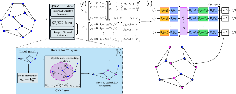
Figure 1: Initialisation techniques for $\mathsf{QAOA}$. (a) This part highlights the difference between the warm-starting techniques (using semi-definite programming (SDP) relaxations [29] or graph neural networks (GNNs)) and Trotterised quantum annealing [30] (TQA). TQA produces initial angles, $\{\boldsymbol{\beta},\boldsymbol{\gamma}\}$, whereas warm-starting techniques initialise the $\mathsf{QAOA}$ state. ‘Init’ here refers to any parameter initialisation scheme. In this work, we choose a specific initialisation technique called the Xavier initialisation [59] for warm-starting techniques. (b) GNNs take an embedding of the initial graph and applies updates to the embeddings based on the neighbours of each node, using an parameterised function, $f_{\boldsymbol{\theta}}$. In this case, the GNN outputs a probability for each node being on either side of the cut. (c) A unified $p$-layer $\mathsf{QAOA}$ circuit for all initialisation schemes. In TQA, fixed choices for angles $\theta,\phi$ initialise vanilla $\mathsf{QAOA}$ with the standard mixer, whereas warm-starting produces an initial state and mixer encoding a probabilistic solution given by the SDP or GNN. Here, $\boldsymbol{x}^{*}$ implicitly encodes the regularisation parameter $\epsilon$ discussed in [29]. Note that both the GNN and $\mathsf{QAOA}$ parameters can be trained in an end-to-end differentiable manner, in contrast to other schemes.

1.1 $\mathsf{QAOA}$ for solving $\mathsf{Max}\text{-}\mathsf{Cut}$

For concreteness in this work, we focus on the discrete optimisation problem known as $\mathsf{Max}\text{-}\mathsf{Cut}$. It involves finding a division (a cut) of the vertices of a (weighted) graph into two sets, which maximises the sum of the weights over all the edges across the vertex subsets. For unweighted graphs, this cut will maximise simply the number of edges across the two subsets.

The problem can be recast to minimising the weighted sum of operators acting on the vertices of a given graph. Mathematically, this can be stated as follows. Given a graph $\mathcal{G}:=\left(\mathcal{V},\mathcal{E}\right)$ with vertices $\mathcal{V}$ and edges $\mathcal{E}=\{(i,j)|i,j\in\mathcal{V}\text{ and }i\neq j\}$, the $\mathsf{Max}\text{-}\mathsf{Cut}$ can be found by minimising the following cost function,

$$\mathsf{C}(\boldsymbol{z})=-\sum_{\langle i,j\rangle\in\mathcal{E}}w_{ij}(1-z_{i}z_{j})$$ (1)

where $\boldsymbol{z}:=z_{1}z_{2}\dots z_{n}$ are variables for each vertex, $i$, such that $z_{i}\in\{+1,-1\}$ and $w_{ij}$ is the corresponding weight of the edge between vertices $i$ and $j$. In this case, the value (sign) of $z_{i}$ determines on which side of the cut the node resides. The $\mathsf{Max}\text{-}\mathsf{Cut}$ problem is a canonical NP-complete problem [60], meaning there is no known efficient polynomial time algorithm in general. Further, $\mathsf{Max}\text{-}\mathsf{Cut}$ is also known to be APX-hard [61], meaning there is also no known polynomial time approximate algorithm. The current best known polynomial time approximate classical approach is the Goemans-Williamson (GW) algorithm which is able to achieve an approximation ratio, $r\approx 0.878$, where:

$$r =\frac{\text{Approximate cut}}{\text{Optimal cut}}$$ (2)

$$=\frac{2}{\pi}\left(\underset{0\leq\theta\leq\pi}{\text{min}}\frac{\theta}{1-\cos\theta}\right)\approx 0.878$$ (3)

Assuming the unique games conjecture (UGC) [62, 63] classically, then the GW algorithm achieves the best approximation ratio for $\mathsf{Max}\text{-}\mathsf{Cut}$. Without this conjecture, it has been proven that it is NP-hard to approximate the $\mathsf{Max}\text{-}\mathsf{Cut}$ value with an approximation ratio better than $\smash{\frac{16}{17}\approx 0.941}$.

To address $\mathsf{Max}\text{-}\mathsf{Cut}$ quantum mechanically, one can quantise the cost function Eq. (1) by replacing the variables with operators, $z_{i}\rightarrow\mathsf{Z}_{i}$, where $\mathsf{Z}$ is the Pauli-$\mathsf{Z}$ matrix. The cost function can now be described with a Hamiltonian:

$$H_{\mathsf{C}}(\boldsymbol{z})=\sum_{\langle i,j\rangle\in\mathcal{E}}w_{ij}(1-\mathsf{Z}_{i}\mathsf{Z}_{j})$$ (4)

where the actual cost - corresponding to the cut size - is extracted as the expectation value of this Hamiltonian with respect to a quantum state, $\ket{\psi}$:

$$\mathsf{C}(\boldsymbol{z}):=-\bra{\psi}H_{\mathsf{C}}\ket{\psi}$$ (5)

The goal of a quantum algorithm is then to find the ground state, $\ket{\psi}_{G}:=\text{arg}\text{min}_{\ket{\psi}}\bra{\psi}H_{\mathsf{C}}\ket{\psi}$, i.e. the state which minimises the energy of the Hamiltonian, $H_{\mathsf{C}}$. Constructing the Hamiltonian as in Eq. (4), ensures that the minimum energy state is exactly the state encoding the $\mathsf{Max}\text{-}\mathsf{Cut}$ of the problem graph:

$$\ket{\psi}_{G}=\ket{\psi}_{\mathsf{Max}\text{-}\mathsf{Cut}}$$ (6)

However, since the $\mathsf{Max}\text{-}\mathsf{Cut}$ problem is NP-Hard, we expect that finding this ground state, $\ket{\psi}_{\mathsf{Max}\text{-}\mathsf{Cut}}$, will also be hard in general. The $\mathsf{QAOA}$ algorithm attempts to solve this by initialising with respect to an easy Hamiltonian (also called a ‘mixer’ Hamiltonian):

$$H_{\mathsf{M}}=\sum_{i=1}^{n}\mathsf{X}_{i}$$ (7)

which has as an eigenstate the simple product state, $\ket{\psi}_{\text{init}}=\ket{+}^{\otimes n}=\mathsf{H}\ket{0}^{\otimes n}$ where $\mathsf{X}$ and $\mathsf{H}$ are the Pauli-$\mathsf{X}$ and Hadamard operators respectively. This can be viewed as an initialisation which is a superposition of all possible candidate solutions. The $\mathsf{QAOA}$ then attempts to simulate adiabatic evolution from $\ket{\psi}_{\text{init}}$ to the target state $\ket{\psi}_{\mathsf{Max}\text{-}\mathsf{Cut}}$ by an alternating bang-bang application of two unitaries derived from the Hamiltonians, Eq. (4), Eq. (7), which are respectively:

$$U_{\mathsf{C}}(\gamma)=e^{-i\gamma H_{\mathsf{C}}}\leavevmode\nobreak\ \text{ and }\leavevmode\nobreak\ U_{\mathsf{M}}(\beta)=e^{-i\beta H_{\mathsf{M}}}$$ (8)

In the $\mathsf{QAOA}$, the parameters, $\gamma,\beta$, are trainable, and govern the length of time each operator is applied for. These two unitaries are alternated in $p$ ‘layers’ acting on the initial state, so the final state is prepared using $2p$ parameters, $\{\boldsymbol{\beta},\boldsymbol{\gamma}\}:=\{\beta_{1},\beta_{2},\dots,\beta_{p},\gamma_{1},\gamma_{2},\dots,\gamma_{p}\}$:

$$\ket{\psi_{\boldsymbol{\beta},\boldsymbol{\gamma}}}=U_{\mathsf{M}}(\beta_{p})U_{\mathsf{C}}(\gamma_{p})\dots U_{\mathsf{M}}(\beta_{1})U_{\mathsf{C}}(\gamma_{1})\ket{+}^{\otimes n}$$ (9)

Optimising the parameters, $\{\boldsymbol{\beta},\boldsymbol{\gamma}\}$ serves as a proxy for finding the ground state, and so we aim that after a finite depth, $p$, we achieve a state $\ket{\psi_{\boldsymbol{\beta},\boldsymbol{\gamma}}}$ which is close to the target state $\ket{\psi}_{\mathsf{Max}\text{-}\mathsf{Cut}}$.

2 Initialising the $\mathsf{QAOA}$

Since searching over the non-convex parameter landscape for an optimal setting of the $\{\boldsymbol{\gamma},\boldsymbol{\beta}\}$ parameters directly on quantum hardware may be expensive and/or challenging, any attempts to initialise the $\mathsf{QAOA}$ parameters near a candidate solution are extremely valuable as the algorithm would then begin its search from an already good approximate solution. Such approaches are dubbed as ‘warm-starts’ [29], in contrast to ‘cold-starts’. One could consider a cold-start to be a random initialisation of $\{\boldsymbol{\gamma},\boldsymbol{\beta}\}$, or by using an initial state which encodes no problem information, e.g. $\ket{+}^{\otimes n}$, as in vanilla $\mathsf{QAOA}$. In this work, we refer to cold-start as the latter, and ‘random initialisation’ to mean a random setting of the parameters, $\{\boldsymbol{\gamma},\boldsymbol{\beta}\}$. We first revisit and summarise two previous approaches [29, 30], before presenting our approach to $\mathsf{QAOA}$ initialisation. We illustrate these previous initialisation approaches in Fig. 1, which we review briefly in Section 2.1 and Section 2.2, and also our approach based on graph neural networks, which we introduce in Section 3. For simplicity, we focus on the simplest version of $\mathsf{QAOA}$, but the methods could be extended to other variants, for example recursive $\mathsf{QAOA}$ (RQAOA) [29, 64, 65].

2.1 Continuous relaxations

The first approach of [29] proposed a warm-start for $\mathsf{QAOA}$ method which can be applied to $\mathsf{Max}\text{-}\mathsf{Cut}$ as a special case of a quadratic unconstrained binary optimisation (QUBO) problem. In this work, two sub-approaches were discussed. The first converts the QUBO into its continuous quadratic relaxation form which is efficiently solvable and directly uses the output of this relaxed problem to initialise the $\mathsf{QAOA}$ circuit. The second approach applies the random-hyperplane rounding method of the GW algorithm to generate a candidate solution for the QUBO. For $\mathsf{Max}\text{-}\mathsf{Cut}$, this QUBO can be written in terms of the graph Laplacian, $\mathcal{L}_{\mathcal{G}}=\mathcal{D}-\mathcal{A}$ (where $\mathcal{D}$ is the diagonal degree matrix, and $\mathcal{A}$ is the adjacency matrix of $\mathcal{G}$) as follows (we utilise this form later in this work):

$$\max_{\boldsymbol{z}\in\{-1,1\}^{n}}\boldsymbol{z}^{T}\mathcal{L}_{\mathcal{G}}\boldsymbol{z}$$ (10)

However, by removing the requirement that each $\boldsymbol{z}_{i}$ is binary, one can obtain an efficiently solvable continuous relaxation that can serve as warm-start for solving Eq. (10). Since $\mathcal{L}_{\mathcal{G}}$ is a positive semidefinite (PSD) matrix, the relaxed form can be trivially written as,

$$\max_{\boldsymbol{x}\in[0,1]^{n}}(2\boldsymbol{x}-1)^{T}\mathcal{L}_{\mathcal{G}}(2\boldsymbol{x}-1),$$ (11)

using the translation $\boldsymbol{z}_{i}\in\{-1,1\}\rightarrow\boldsymbol{z}_{i}=(2\boldsymbol{x}_{i}-1),\leavevmode\nobreak\ \boldsymbol{x}_{i}\in\{0,1\}$ and then allowing $\boldsymbol{x}_{i}$ to be continuous in this interval. If the matrix in the QUBO is not PSD however, then one can obtain another continuous relaxation, as a semidefinite programme (SDP) [66, 29]. The output of this optimisation is a real vector $\boldsymbol{x}^{*}$ which, when a rounding procedure is performed (i.e. the GW algorithm), is a candidate solution for the original $\mathsf{Max}\text{-}\mathsf{Cut}$. In order to use this relaxed solution to initialise $\mathsf{QAOA}$, Ref. [29] also demonstrated that the initial state from Eq. (9) and the mixer Hamiltonian Eq. (7) must also be altered as:

$$\begin{split}&\ket{\psi}_{\text{init}}^{\text{CS}}=\ket{+}^{\otimes n}\rightarrow\ket{\psi}_{\text{init}}^{\text{WS}}=\bigotimes\limits_{i=1}^{n}\mathsf{R}_{y}(\boldsymbol{\theta}_{i})\ket{0}^{\otimes n}.\\ &H_{\mathsf{M}}\rightarrow\sum\limits_{i=1}^{n}H^{\text{WS}}_{\mathsf{M},i},\\ &H^{\text{WS}}_{\mathsf{M},i}=\left(\begin{array}[]{cc}2\boldsymbol{x}^{*}_{i}-1&-2\sqrt{\boldsymbol{x}_{i}^{*}(1-\boldsymbol{x}_{i}^{*})}\\ -2\sqrt{\boldsymbol{x}_{i}^{*}(1-\boldsymbol{x}_{i}^{*})}&1-2\boldsymbol{x}^{*}_{i}\end{array}\right)\end{split}$$ (12)

where $\boldsymbol{\theta}_{i}=2\sin^{-1}(\sqrt{\boldsymbol{x}^{*}_{i}})$. One can immediately see that $\ket{\psi}_{\text{init}}^{\text{WS}}$ is the ground state of $H_{\mathsf{M}}$ with eigenvalue $-n$. One possible issue that may arise with this warm-start is if the relaxed solution $\boldsymbol{x}_{i}^{*}$ is either 0 or 1. When this happens, the qubit $i$ would be initialised to state $\ket{0}$ or $\ket{1}$, respectively. This means the qubit would be unaffected by the problem Hamiltonian Eq. (4) which only contains Pauli Z terms. To account for this possibility,  [29] modifies $\boldsymbol{\theta}_{i}$ in Eq. (12) with a regularisation parameter, $\epsilon\in[0,0.5]$ if the candidate solution, $\boldsymbol{x}^{*}_{i}$ is too close to $0$ or $1$.

Examining Fig. 1, this initialisation scheme is achieved by setting the angles in the initial state, $\boldsymbol{\varphi}_{i}=0$ and $\boldsymbol{\theta}_{i}=2\sin^{-1}(\sqrt{\boldsymbol{x}^{*}_{i}})\leavevmode\nobreak\ \forall i$ where the initial state can be expressed as $\ket{\psi}_{\text{init}}^{\text{WS}}=\bigotimes\mathsf{R}_{x}(\boldsymbol{\varphi}_{i})\mathsf{R}_{y}(\boldsymbol{\theta}_{i})\ket{0}^{\otimes n}$. The ‘Init’ in this figure implies that one is free to choose any $\mathsf{QAOA}$ parameter initialisation method as this warm-start approach only modifies the input state and the mixer Hamiltonian.

2.2 Trotterised quantum annealing

A second proposed method [30] to initialise $\mathsf{QAOA}$ uses concepts from quantum annealing [67, 68], which is a popular method of solving QUBO problems of the form Eq. (10). $\mathsf{QAOA}$ was proposed as a discrete gate-based method to emulate quantum adiabatic evolution, or quantum annealing. Therefore, one may hope that insights from quantum annealing may be useful in setting the initial angles for the $\mathsf{QAOA}$ circuit parameters. In a method proposed by [30] (dubbed Trotterised quantum annealing (TQA)), one fixes the $\mathsf{QAOA}$ circuit depth, $p$, and sets the parameters as:

$$\boldsymbol{\gamma}_{k}=\frac{k}{p}\delta t\qquad\boldsymbol{\beta}_{k}=\left(1-\frac{k}{p}\right)\delta t$$ (13)

where $k=1,\cdots,p$ and $\delta t$ is a time interval which is a-priori unknown and given as a fraction of the (unknown) total optimal anneal time, $T^{*}$, resulting in $\delta t=T^{*}/p$. The authors of [30] observed an optimal time step value $\delta t$ to be $\approx 0.75$ for 3-regular graphs and $\mathcal{O}(1)$ for other graph ensembles. In [30], the $\mathsf{QAOA}$ was initialised with $\delta t=0.75$ and observed to help avoid local minima and find near-optimum minima close to the global minimum. We also choose this value generically in our numerical results later in the text, although one should ideally pre-optimise the value for each graph instance.

Note that in contrast to the warm-starting method from the previous section, the TQA approach initialises the parameters, $\{\boldsymbol{\beta},\boldsymbol{\gamma}\}$ rather than the initial $\mathsf{QAOA}$ state (and mixer Hamiltonian) which is set as in vanilla $\mathsf{QAOA}$ as $\ket{+}$. Again, revisiting Fig. 1, this initial state can be achieved by choosing $\boldsymbol{\varphi}_{j}=\pi,\boldsymbol{\theta}_{j}=\nicefrac{{\pi}}{{2}},\leavevmode\nobreak\ \forall j$. This is due to the fact that $\mathsf{R}_{y}\left(\nicefrac{{\pi}}{{2}}\right)\mathsf{R}_{x}(\pi)\ket{0}\propto\mathsf{X}\mathsf{R}_{x}\left(\nicefrac{{\pi}}{{2}}\right)\ket{0}=\mathsf{H}\ket{0}=\ket{+}$. Similarly, for the mixer Hamiltonian, we have $\mathsf{R}_{y}\left(\nicefrac{{\pi}}{{2}}\right)\mathsf{R}_{z}(-2\beta_{k})\mathsf{R}_{y}\left(-\nicefrac{{\pi}}{{2}}\right)\propto\mathsf{H}\mathsf{X}\mathsf{R}_{z}(-2\beta_{k})\mathsf{X}\mathsf{H}=\mathsf{H}\mathsf{R}_{z}(2\beta_{k})\mathsf{H}=\mathsf{R}_{x}(2\beta_{k})$, which is the single qubit mixer unitary from vanilla $\mathsf{QAOA}$, up to a redefinition of $\beta_{k}$.

3 Graph neural network warm-starting of $\mathsf{QAOA}$

Now that we have introduced the $\mathsf{QAOA}$, and alternative methods for warm-starting its initial state and/or initial algorithm parameters, let us turn now to our proposed method; the use of graph neural networks. This approach is closest to the relaxation method of Section 2.1 in that the GNN provides an alternative initial state to vanilla $\mathsf{QAOA}$, and so it is to this method which we primarily compare. One of the main drawbacks of using SDP relaxations and the GW algorithm, is that every graph for which the $\mathsf{Max}\text{-}\mathsf{Cut}$ must be found generates a new problem instance to be initialised. However, on the other hand, the GW algorithm comes equipped with performance guarantees (generating an approximate solution within $88\%$ of the optimal answer).

As we shall see, using graph neural networks as an initialiser allows a generalisation across many graph instances at once. Importantly, even increasing the number of qubits will not significantly affect the time complexity of such approaches as it can be interpreted as a learned prior over graphs. We also demonstrate how the model can be trained on a small number of qubits, and still perform well on larger problem instances (size generalisation), a feature not present in any of the previous initialisation methods for $\mathsf{QAOA}$. Furthermore, the incorporation of a differentiable initialisation structure allows the entire pipeline of $\mathsf{QAOA}$ to become end-to-end differentiable, which is particularly advantageous since it makes the problem ameanable to the automatic differentiation functionality of many deep learning libraries [69, 70]. First, let us begin by introducing graph neural networks.

3.1 Graph neural networks

Graph neural networks (GNNs) [71] are a specific neural network model designed to operate on graph-structured data, and typically function via some message passing process across the graph. They are example models in geometric deep learning [72], where one incorporates problem symmetries and invariants into the learning protocol. Examples have also been proposed in the field of quantum machine learning [50, 73, 74, 75]. Specifically, graph neural networks operate by taking an encoding of the input graph describing a problem of interest and outputting a transformed encoding. Each graph node is initially encoded as a vector, which are then updated by the GNN to incorporate information about the relative features of the graph in the node. This is done by taking into account the connections and directions of the edges within the graph, using quantities such as the node degree, and the adjacency matrix. This transformed graph information is then used to solve the problem of interest. There are many possible architectures for how this graph information is utilised in the GNN, including attention based mechanisms [76] or graph convolutions [77] for example, see e.g. Ref. [78] for a review.

In order to transform the feature embeddings, the GNN is trained for a certain number of iterations (a hyperparameter). For a given graph node, $n_{\nu}$, we associate a vector, $\boldsymbol{h}^{n_{\nu}}_{t}$, where $t$ is the current iteration. In the next iteration ($t+1$), to update the vector for node $n_{\nu}$, we first compute some function of the vector embeddings of the nodes in a neighbourhood of $n_{\nu}$, denoted as $\mathcal{N}(n_{\nu})=\{n_{j}\}_{j:n_{j}\sim n_{\nu}}$. A-priori, there is no limitation on how large this neighbourhood can be, making it larger will increase training time and difficulty, but increase representational power. These function values are then aggregated (for example by taking an average) and combined with the node vector (with perhaps a non-linear activation function) at the previous iteration to generate $\boldsymbol{h}^{n_{\nu}}_{t+1}$. Each nodes update increases the information contained relative to a larger subset of nodes in the graph. The collective action of these operations can be described by a parameterised, trainable function, $f_{\boldsymbol{\theta}}(\boldsymbol{h}^{n_{\nu}}_{t},\{\boldsymbol{h}^{n_{j}}_{t}\}_{j:n_{j}\sim n_{\nu}})$ (see Fig. 1), whose parameters, $\boldsymbol{\theta}$, are suitably trained to minimise a cost function. In all cases here, we initialise all the elements of the feature vectors, $\boldsymbol{h}^{n_{\nu}}_{0}$ to be the degree of the node, $n_{\nu}$. For the specific GNN architecture we use in the majority of this work, we choose the line graph neural network (LGNN) [79], shown to be competitive on combinatorial optimisation problems [53]. However we also incorporate the graph convolutional network (GCN) proposed for combinatorial optimisation by [56] in some numerical results in Section 4. We give further details about these two architectures in Appendix A.

Once we have a trained GNN for a certain number of iterations, $T$, we can use the information encoded in $\{\boldsymbol{h}^{n_{j}}_{T}\}_{j}$ for the problem at hand. A simple example would be to attach a multi-layer perception and perform classification on each node, where $\{\boldsymbol{h}^{n_{j}}_{T}\}$ behaves as feature vectors encoding the graph structure. For our purposes, we use these vectors to generate probabilities on the nodes. These are the probabilities that the node is in a given side of the $\mathsf{Max}\text{-}\mathsf{Cut}$, which are then taken as the values $\boldsymbol{x}^{*}$ in warm-started $\mathsf{QAOA}$ circuit and its mixer Hamiltonian Eq. (12).

3.2 Graph neural networks for $\mathsf{Max}\text{-}\mathsf{Cut}$

To attach this probability, there are at least two possible methods one could apply. Firstly, one could consider using reinforcement learning or long short term memories (LSTMs) [80, 81]. These methods generate probabilities in a step-wise fashion by employing a sequential dependency. To train these, one may use a policy gradient method [82] (dubbed as an ‘autoregressive decoding’ approach [83]).

The second (simpler) method is to treat edge independently, and generate the probability of each edge being present in the $\mathsf{Max}\text{-}\mathsf{Cut}$ or not (a ‘non-autoregressive decoding’). This can be formulated as a vector, $\boldsymbol{p}$, where each element corresponds to a node, $n_{\nu}$, generated by applying a softmax to the final output feature vectors of the GNN, $\{\boldsymbol{h}^{n_{j}}_{T}\}_{j}$ [53, 56]:

$$p_{n_{\nu}}(\boldsymbol{\theta})=\frac{\exp\left(\boldsymbol{h}^{n_{\nu},0}_{T}\right)}{\sum_{j\in\{0,1\}}\exp\left(\boldsymbol{h}^{n_{\nu},j}_{T}\right)}$$ (14)

In [53], for each node, $n_{\nu}$, the final output is the two dimensional vector $[\boldsymbol{h}^{n_{\nu},0}_{T},\boldsymbol{h}^{n_{\nu},1}_{T}]$, constructed as the output of a final two-output linear layer. The probability for each node is then taken as one of these outputs (say $j=0$) via the softmax in Eq. (14) and then used in the cost function described in the next section.

3.2.1 Unsupervised training

Now that we have defined the structure and output of the GNN, it must be suitably trained. One approach is to use supervised training, however this may require a large number of example graphs to serve as the ground truth. Instead, following [53, 56], we opt for an unsupervised approach, bypassing the need for labels. To do so, we choose the cost function as [53], which is given by the $\mathsf{Max}\text{-}\mathsf{Cut}$ QUBO itself in terms of the graph Laplacian (Eq. (10)):

$$\mathsf{C}_{\text{GNN}}=-\min_{\boldsymbol{\theta}}\frac{1}{T}\sum\limits_{t=1}^{T}(-\mathsf{C}^{t}_{\text{GNN}}(\boldsymbol{\theta}))$$ (15)

$$\mathsf{C}^{t}_{\text{GNN}}(\boldsymbol{\theta})=\frac{1}{4}(2\boldsymbol{p}-1)^{T}\mathcal{L}_{\mathcal{G}}(2\boldsymbol{p}-1)$$ (16)

where $\boldsymbol{p}\in[0,1]^{n}$ is the probability vector from the GNN Eq. (14). In Eq. (15), we define the cost function as an average over a training set of $T$ graphs, $\{\mathcal{G}_{t}\}_{t=1}^{T}$. Note, that the graphs in the training set do not have to be the same size as the graphs of interest; the GNN can be trained on an ensemble of graphs of different sizes, or graphs which are strictly smaller (or larger) than the test graph. We utilise this feature to improve GNN training in Section 4.1 and to demonstrate the generalisation capabilities of the GNN in Section 4.2. See Ref. [56] for how the cost function and GNN structure could be adapted to alternate QUBO type problems.

4 Initialisation numerical results

Let us first study the impact of the initialisation schemes discussed above on the $\mathsf{QAOA}$ numerically. In all of the below, the approximation ratio, $r$, will be the figure of merit. We also use Xavier initialisation [59] for the $\mathsf{QAOA}$ parameters in all cases except for the TQA initialisation method. This initialises each parameter from a uniform distribution over an interval depending on the number of parameters in the $\mathsf{QAOA}$ circuit.

Figure 2: Success probability of the graph neural network on $3$-regular graphs for $\mathsf{Max}\text{-}\mathsf{Cut}$. Histogram shows the number of graphs on which GNN $\mathsf{QAOA}$ versus cold-start $\mathsf{QAOA}$ can achieve a certain ratio of the optimal cut. Here, we set $p=5$ and $n=12$ qubits and generate the percentages over $50$ random graphs. The GNN initialised version is able to generate larger cut values than the vanilla version of $\mathsf{QAOA}$.

We begin by benchmarking the graph neural network $\mathsf{QAOA}$ against a random cold start initialisation for the two architectures discussed above, the line graph neural network (LGNN) and the graph convolutional network (GCN). To demonstrate feasibility, Fig. 2 shows the success probability of the vanilla (cold-started) $\mathsf{QAOA}$ against the (LGNN-)$\mathsf{QAOA}$ initialisation over $50$ random $3$-regular graphs with $12$ qubits and $p=5$ $\mathsf{QAOA}$ depth. We observe the GNN-$\mathsf{QAOA}$ is capable of generating larger cuts on average than the vanilla version.

Next, Fig. 3 compares the approximation ratio directly output by the GNN, against the GNN initialised solution which is then further optimised by $\mathsf{QAOA}$. To generate discrete $\mathsf{Max}\text{-}\mathsf{Cut}$ solutions from the GNN probability vectors, we choose the same simple rounding scheme as [56], assigning $\boldsymbol{x}_{i}^{*}=\text{int}(\boldsymbol{p}_{i})\in\{0,1\}$ for each node, $i$. We leave the incorporation and comparison of more complex rounding techniques to future work.

We first plot as function of qubit number (graph size), for $\mathsf{QAOA}$ depths scaling proportionally with the number of qubits ($p=3n/4$ in (a) and $p=n/2$ in (b)). We see that the GNN $\mathsf{QAOA}$ outperforms both the GNN and vanilla $\mathsf{QAOA}$ individually. This advantage is more pronounced at lower relative depth, but is diminished at higher depth. This is confirmed by Fig. 3(c) where we fix the qubit number at $16$ and plot the results as a function of $\mathsf{QAOA}$ depth. However, since the depth of quantum circuits is limited by decoherence in NISQ devices, the advantage of the GNN in the low-depth regime is promising. Finally, since we observe in these results that the LGNN appears to outperform the GCN architecture (due to the more complex message passing functionality), we opt to use the former primarily in the remainder of this work. However, for larger problem sizes, the LGNN may be less scalable [56].

(a)

(b)

(c)

Figure 3: Performance of the graph neural network on $3$-regular graphs for $\mathsf{Max}\text{-}\mathsf{Cut}$. We compare the $\mathsf{Max}\text{-}\mathsf{Cut}$ approximation ratios achieved with LGNN/GCN initialisation versus cold-start (vanilla) $\mathsf{QAOA}$. We also plot the raw values outputted by the LGNN with a simple rounding scheme. In (a), the $\mathsf{QAOA}$ depth is set to be $p=3n/4$, while in (b), $p=n/2$. Each datapoint is generated via $1000$ runs of the LGNN/GCN on random instances of $3$-regular graphs, of the appropriate size to the number of qubits. Finally, in (c), we fix the number of qubits to be $16$ and plot each method as a function of the $\mathsf{QAOA}$ depth, demonstrating monotonic improvement as a function of $p$. Each datapoint is generated via $1000$ runs of the LGNN/GCN on random instances of $3$-regular graphs, of the appropriate size to the number of qubits.

4.1 Graph neural network versus SDP relaxations

Next, we benchmark the GNN against the SDP relaxation approach directly in Fig. 4. We begin in Fig. 4(a) by comparing the quality of the $\mathsf{Max}\text{-}\mathsf{Cut}$ solution produced by the GW algorithm ($r_{\text{GW}}$) against the solution from the (line-)GNN ($r_{\text{GNN}}$). We observe comparable quality between the two methods (as remarked previously [56]) with the GNN generating solutions which are between $85$-$90\%$ the quality of the GW algorithm. However, we note that for these small graph instances, the training set becomes saturated as all possible $3$-regular graphs eventually appear. Naively increasing the size (say from $N_{\text{train}}=1000$ to $N_{\text{train}}=5000$) of training set with graphs of the same size as the test case does not improve performance of the GNN dramatically. Therefore, in order to non-trivially increase the amount of training data, we include graphs of different sizes (taking $N_{\text{train}}=5000$ graphs which are $1\times$-$5\times$ the size of the test graph) in the training set. Doing so increases the performance ratio of GNN over GW to $\sim 95\%$, at the expense of a greater training time. However, if we then examine Fig. 4(b) and Fig. 4(c), then the tradeoff we are making becomes apparent. With a small sacrifice in solution quality, the GNN (once trained) is able to generate candidate solutions significantly faster than SDP relaxations and the GW algorithm.

Firstly, in Fig. 4(b) and show that the inference time (time to produce a warm-started solution) is significantly higher with the SDP relaxation method than using a trained GNN. For this plot we focus graphs relevant to the $\mathsf{QAOA}$ problem sizes we study in this paper. Next, we show in Fig. 4(c) how the GNNs speed advantage enables the scalable production of warm-started solutions for $\mathsf{QAOA}$ into millions of variables, far beyond the capability of near term quantum devices. Specifically, we reproduce the results of [56] comparing the full time taken by the SDP relaxation and the GW algorithm against the GCN architecture (even including training time) to solve $\mathsf{Max}\text{-}\mathsf{Cut}$ (see [56] for details). The runtime of the GW algorithm is limited by the interior-point method used to solve SDPs which scales as $\widetilde{\mathcal{O}}(n^{3.5})$ [56]. In Section 4.2, we take this even further and demonstrate how the GNN approach is able to generalise not only across test graph instances of the same size as in the training set, but also to larger test graph instances, which is a feature clearly not possible via the relaxation method.

As a final comparison, we compare the GNN initialisation technique against all other techniques in Fig. 5. We compare against the warm-starting technique using relaxations of [29] (‘Warm-start’), and the Trotterised quantum annealing (‘TQA’) based approach of [30], as a function of depth and training epochs.

(a)

(b)

(c)

Figure 4: Time versus quality tradeoff between GNN versus relaxation initialisation methods. (a) $\mathsf{Max}\text{-}\mathsf{Cut}$ approximation ratios generated by GNN and the continuous relaxation (without $\mathsf{QAOA}$), as a function of graph size. $r_{j}$ is the approximation ratio generated by method $j\in\{\text{GW},\text{GNN}\}$. We use a simple rounding technique to generate the discrete values from the soft outcomes from the (line-)GNN (see main text) and plot results for $1000$ and $5000$ training graphs. (b) Comparison of time to produce a warm-start taken by relaxation initialisation versus (line-)GNN initialisation as a function of qubit number, averaged over $10$ random graph instances. The GNN enables much faster inference for $\mathsf{Max}\text{-}\mathsf{Cut}$. This does not include pre-training time for the GNN, but as an example, training on $1000$ graphs for $18$ qubits takes only $6$ minutes for the LGNN. Finally, (c) reproduces results taken from [56] demonstrating the scalability of the GNN initialisation (for the GCN) over solving the SDP relaxation with the GW algorithm. The GNN can provide warm-starts for $\mathsf{QAOA}$ on graphs with millions of nodes. Note, these plots do not include $\mathsf{QAOA}$ runtime after the warm-start.

(a)

(b)

Figure 5: Comparison of all initialisation techniques. We use $3$-regular graphs over $8$ qubits and for TQA we choose $\delta t=0.75$ as in [30]. (a) Convergence of initialisations as a function of training iteration. The depth of QAOA is fixed to $5$. (b) Comparison of initialisations as a function of $\mathsf{QAOA}$ depth $p$. We plot the average for each method over $10$ runs.

4.2 Generalisation capabilities of GNNs

A key feature of using neural networks for certain tasks is capability to generalise. This generalisation ability is one of the driving motivations behind machine learning, and tests the ability of an algorithm to actually learn (rather than just memorise a solution). Similarly, we can test the generalisation ability of GNNs in warm-starting the $\mathsf{QAOA}$. To do so, we train instantiations of GNNs on small graph instances, and then directly apply them to larger test instances. We test this for examples of between $6$ to $14$ nodes in Table 1. Here, we see this generalisation feature directly, as the GNN is capable of performing well on graphs larger than those in the training set. Note a related generalisation behaviour was demonstrated via meta-learning [50, 51] for the parameters of a variational circuit. The work of [50] utilises recurrent neural networks (we revisit this strategy in Section 5.3.2) for training the $\mathsf{QAOA}$, but generalisation in this case was possible due to the structure of the algorithm and parameter concentration [18]. The FLexible Initializer for arbitrarily-sized Parametrized quantum circuits (FLIP) [51], also has related parameters generalisation capabilities, which would be interesting to compare and incorporate with warm-starting initialisers in future work.

The rows in Table 1 correspond to the graph size on which the model was trained, and the columns correspond to the graph size on which the GNN was then tested. For example, both training and testing on graphs with $10$ nodes gives an approximation ratio of $\approx 0.93$, whereas if we train the GNN using only graphs of $6$ nodes, there is no drop in performance. In contrast, if we reduce from $14$ to $6$ training nodes, we only see a drop in the approximation ratio of $7\%$. Again, we mention the limitation to small problem sizes due to the $\mathsf{QAOA}$ circuit simulation overhead. As with the discussions above, it has been observed that GNNs trained on $30$ node graphs have the ability to generalise to $300$ nodes and larger [53, 56]. Note that this generalisation is the reverse situation to that in Fig. 4(a), where we include larger graphs in the training set to improve solution quality in smaller graphs, rather than including larger graphs in the test set, as we do here.

8 10 12 14 6 0.91 0.93 0.89 0.89 8 0.93 0.92 0.89 0.91 10 0.93 0.90 0.89 12 0.90 0.89 14 0.96

Table 1: Value of approximation ratio, $r$, as a function of training and test graph size. In each case, both the train and test set consists of $1000$ random graphs of the appropriate sizes. Bold indicates the instances where the train graph size is the same as the test size.

5 Optimisation of the $\mathsf{QAOA}$

Now, we move to the second focus of this work, which is a comparison between a wide range of different optimisers which can be used to train the $\mathsf{QAOA}$ when solving the $\mathsf{Max}\text{-}\mathsf{Cut}$ problem. A large variety of optimisers for VQAs have been proposed in the literature, and each has their own respective advantages and disadvantages when solving a particular problem. Due to the hybrid quantum-classical nature of these algorithms, many of optimisation techniques have been taken directly from classical literature in, for example, the training of classical neural networks. However, due to the need to improve the performance of near term quantum algorithms, there has also been much effort put into the discovery of quantum-aware optimisers, which may include many non-classical hyperparameters including, for example, the number of measurement shots to be taken to compute quantities of interest from quantum states [84, 85]. In the following sections, we implement and compare a number of these optimisers. We begin by evaluating gradient-based and gradient-free optimisers in Section 5. We then compare quantum and classical methods for simultaneous perturbation stochastic optimisation in Section 5.2, which typically have lower overheads than the gradient-free or gradient-based optimisers since all parameters are updated in a single optimisation step, as opposed to parameter-wise updates. Finally, we then implement some neural network based optimisers in Section 5.3 which operate via reinforcement learning and the meta-learning optimiser mentioned above. In all of the above cases, we use vanilla stochastic gradient descent optimisation as a benchmark.

5.1 Gradient-based versus gradient-free optimisation

For a given parameterised quantum circuit instance, equipped with parameters at iteration (epoch), $t$, $\boldsymbol{\theta}^{t}$, the parameters at iteration $t+1$ are given by an update rule:

$$\boldsymbol{\theta}^{t+1}=\boldsymbol{\theta}^{t}-\Delta\mathsf{C}(\boldsymbol{\theta}^{t})$$ (17)

$\Delta\mathsf{C}(\boldsymbol{\theta}^{t})$ is the update rule, which contains information about the cost function to be optimised at epoch $t$, $\mathsf{C}(\boldsymbol{\theta}^{t})$. In gradient-based optimisers, the update contains information about the gradients of $\mathsf{C}(\boldsymbol{\theta}^{t})$ with respect to the parameters, $\boldsymbol{\theta}^{t}$. In contrast, gradient-free (or zeroth order) optimisation methods use only information about $\mathsf{C}(\boldsymbol{\theta}^{t})$ itself. One may also incorporate second-order derivative information also, which tend to outperform the previous methods, but are typically more expensive as a result. In the following, we test techniques which fall into all of these categories, for a range of qubit numbers and $\mathsf{QAOA}$ depths.

A general form of this update rule when incorporating gradient information can be written as:

$$\boldsymbol{\theta}^{t+1}=\boldsymbol{\theta}^{t}-\eta(t,\boldsymbol{\theta})\boldsymbol{g}(\boldsymbol{\theta})^{-1}\nabla\mathsf{C}(\boldsymbol{\theta}^{t})$$ (18)

where $\eta(t,\boldsymbol{\theta})$ is a learning rate, which determines the speed of convergence, and may depend on the previous parameters, $\boldsymbol{\theta}$ and $t$. The quantity $\boldsymbol{g}(\boldsymbol{\theta})\in\mathbb{R}^{d\times d}$ is a metric tensor, which incorporates information about the parameter landscape. This tensor can be the classical, or quantum Fisher information (QFI) for example. In the case of the latter, the elements of $\boldsymbol{g}(\boldsymbol{\theta})$ when dealing with a parameterised state, $\ket{\psi_{\boldsymbol{\theta}}}$ are given by:

$$\boldsymbol{g}_{ij}(\boldsymbol{\theta}):=\text{Re}\bigg{\{}\bigg{\langle}\frac{\partial\psi_{\boldsymbol{\theta}}}{\partial\boldsymbol{\theta}_{i}}\bigg{|}\frac{\partial\psi_{\boldsymbol{\theta}}}{\partial\boldsymbol{\theta}_{j}}\bigg{\rangle}\\ \left.-\bigg{\langle}\frac{\partial\psi_{\boldsymbol{\theta}}}{\partial\boldsymbol{\theta}_{i}}\bigg{|}{\psi_{\boldsymbol{\theta}}}\bigg{\rangle}\bigg{\langle}\psi_{\boldsymbol{\theta}}\bigg{|}\frac{\partial\psi_{\boldsymbol{\theta}}}{\partial\boldsymbol{\theta}_{j}}\bigg{\rangle}\right\}$$ (19)

In this form, the gradient update Eq. (18) updates the parameters according to the quantum natural gradient (QNG) [86].

If we further simplify by taking $\boldsymbol{g}=\mathds{1}$ to be the identity and choosing different functions for $\eta(\boldsymbol{\theta},t)$, we recover many popular optimisation routines such as Adam [87] or Adadelta [88], which incorporates notions such as momentum into the update rule, and makes the learning rate time-dependent. Such behaviour is desired to, for example, allow the parameters to make large steps at the beginning of optimisation (when far from the target), and take smaller steps towards the latter stage when one is close to the optimal solution. The simplest form of gradient descent is vanilla, which takes $\eta(\boldsymbol{\theta},t):=\eta$ to be a constant. The ‘stochastic’ versions of gradient descent use an approximation of the cost gradient computed with only a few training examples. In Fig. 6, we begin by comparing some examples of the above gradient-based optimisation rule (specifically using QNG, Adam and RMSProp) to a gradient-free method (COBYLA) [89]. We also add a method known as model gradient descent (MGD) which is a gradient-based method introduced by [37] that involves quadratic model fitting as a gradient estimation (see Appendix A of [90] for pseudocode). The results are shown in Fig. 6 for $\mathsf{Max}\text{-}\mathsf{Cut}$ on $3$ regular graphs for up to $14$ qubits. We observe that optimisation using the QNG outperforms other methods, however it does so with a large resource requirement, which is needed to compute the quantum fisher information (QFI) using quantum circuit evaluations.

Figure 6: Gradient-based versus gradient-free optimisers. We set the depth of $\mathsf{QAOA}$ depth to $p=4$ and vary the number of qubits. All optimisers have been run $10$ times and average values have been plotted.

We next examine the convergence speed of the ‘quantum-aware’ QNG optimiser, versus the standard Adam and RMSProp in Fig. 7. Again, QNG significantly reduces convergence time, but again at the expense of being a more computationally taxing optimisation method [86].

Figure 7: Comparison of optimisers relative to convergence speed. We fix $\mathsf{QAOA}$ depth at $p=6$ with $14$ qubits.

5.2 Simultaneous perturbation stochastic approximation optimisation

From the above, using the QNG as an optimisation routine is very effective, but it has a large computational burden due to the evaluation of the quantum Fisher information. A strategy to bypass this inefficiency was proposed by [91], who suggested combining the QNG gradient with the simultaneous perturbation stochastic approximation (SPSA) algorithm. This algorithm is an efficient method to bypass the linear scaling in the number of parameters using the standard parameter shift rule [7, 92], to compute quantum gradients. For example, in the expression Eq. (18) when restricted to vanilla gradient descent, one gradient term must be computed for each of the $d$ ($d=2p$ in the case of the $\mathsf{QAOA}$) parameters. In contrast, SPSA approximates the entire gradient vector by choosing a random direction in parameter space and estimating the gradient in this direction using, for example, a finite difference method. This requires a constant amount of computation relative to the number of parameters. To incorporate the quantum Fisher information, [91] to SPSA actually uplifts a second order version of SPSA (called $2$-SPSA), which exploits the Hessian of the cost function to be optimised. The update rules for $1$-, $2$-SPSA and QN-SPSA are given by:

$$\boldsymbol{\theta}^{t+1} =\boldsymbol{\theta}^{t}-\eta\times\begin{cases}\widetilde{\nabla}\mathsf{C}(\boldsymbol{\theta}^{t})&\quad 1\text{-SPSA}\\ \widetilde{H}^{-1}(\boldsymbol{\theta}^{t})\widetilde{\nabla}\mathsf{C}(\boldsymbol{\theta}^{t})&\quad 2\text{-SPSA}\\ \widetilde{\boldsymbol{g}}^{-1}(\boldsymbol{\theta}^{t})\widetilde{\nabla}\mathsf{C}(\boldsymbol{\theta}^{t})&\quad\text{QN-SPSA}\end{cases}$$ (20)

where stochastic approximation to the Hessian, $\widetilde{H}(\boldsymbol{\theta})$, and the quantum Fisher information are given by:

$$\widetilde{H}^{t}:=-\frac{1}{2}\frac{\delta\mathsf{C}}{2\epsilon^{2}}\frac{\Delta_{1}^{t}(\Delta_{2}^{t})^{T}+\Delta_{2}^{t}(\Delta_{1}^{t})^{T}}{2}$$ (21)

$$\delta\mathsf{C}:=\mathsf{C}(\boldsymbol{\theta}^{t}+\epsilon\Delta_{1}^{t}+\epsilon\Delta_{2}^{t})-\mathsf{C}(\boldsymbol{\theta}^{t}+\epsilon\Delta_{1}^{t})\\ -\mathsf{C}(\boldsymbol{\theta}^{t}-\epsilon\Delta_{1}^{t}+\epsilon\Delta_{2}^{t})+\mathsf{C}(\boldsymbol{\theta}^{t}-\epsilon\Delta_{1}^{t})$$ (22)

and

$$\widetilde{\boldsymbol{g}}^{t}=-\frac{1}{2}\frac{\delta F}{2\epsilon^{2}}\frac{\Delta_{1}^{t}(\Delta_{2}^{t})^{T}+\Delta_{2}^{t}(\Delta_{1}^{t})^{T}}{2}$$ (23)

$$\delta F:=F(\boldsymbol{\theta}^{t},\boldsymbol{\theta}^{t}+\epsilon\Delta_{1}^{t}+\epsilon\Delta_{2}^{t})-F(\boldsymbol{\theta}^{t},\boldsymbol{\theta}^{t}+\epsilon\Delta_{1}^{t})\\ -F(\boldsymbol{\theta}^{t},\boldsymbol{\theta}^{t}-\epsilon\Delta_{1}^{t}+\epsilon\Delta_{2}^{t})+F(\boldsymbol{\theta}^{t},\boldsymbol{\theta}^{t}-\epsilon\Delta_{1}^{t})$$ (24)

respectively. Here, $F(\boldsymbol{\theta},\boldsymbol{\theta}+\boldsymbol{\alpha})=|\langle{\psi_{\boldsymbol{\theta}}}|\psi_{\boldsymbol{\theta}+\boldsymbol{\alpha}}\rangle|^{2}$ is the fidelity between the parameterised state prepared with angles, $\boldsymbol{\theta}$, and a ‘shifted’ version with angles $\boldsymbol{\theta}+\boldsymbol{\alpha}$. The quantities $\Delta_{1},\Delta_{2}$ are uniformly random vectors sampled over $\{-1,1\}^{d}$. Also, $\epsilon$ is a small constant arising from finite differencing approximations of the gradient, for example, we approximate the true gradient, $\nabla\mathsf{C}(\boldsymbol{\theta})$ by $\widetilde{\nabla}\mathsf{C}(\boldsymbol{\theta})$, given by:

$$\widetilde{\nabla}\mathsf{C}(\boldsymbol{\theta}^{t}):=\frac{\mathsf{C}(\boldsymbol{\theta}^{t}+\epsilon\Delta^{t})-\mathsf{C}(\boldsymbol{\theta}^{t}-\epsilon\Delta^{t})}{2\epsilon}\Delta^{t}$$ (25)

We compare all these three perturbation methods in Fig. 8 against SGD once again, with a fixed learning rate of $\eta=0.01$. Notice that SGD performs comparably to $1$-SPSA, but with the expense of more cost function evaluations.

(a)

(b)

(c)

Figure 8: Simultaneous perturbation stochastic approximation ($1$-, $2$- and QN-SPSA) for $\mathsf{Max}\text{-}\mathsf{Cut}$ with $\mathsf{QAOA}$. Plots show approximation ratio as a function of (a) depth (qubit number fixed at $10$), (b) number of qubits ($\mathsf{QAOA}$ depth is fixed to $p=5$) and (c) training iteration (qubit number and $\mathsf{QAOA}$ depth fixed to $10$ and $7$ respectively). In all cases, the average is taken over $10$ independent optimisation runs.

5.3 Neural optimisation

In this section, we move to a different methodology to find optimal $\mathsf{QAOA}$ parameters than those presented in the previous section. Specifically, as with the incorporation of graph neural networks in the initialisation of the algorithms, we can test neural network based methods for the optimisation itself. Specifically, we test two proposals given in this literature to optimise parameterised quantum circuits. The first, based on a reinforcement learning approach, uses the method of [33]. The second is derived from using meta learning to optimise quantum circuits, proposed by [50]. Both of these approaches involve neural networks outputting the optimised parameters by either predicting the update rule or directly predicting the $\mathsf{QAOA}$ parameters.

5.3.1 Reinforcement learning optimisation

The work of [33] frames the $\mathsf{QAOA}$ optimisation as a reinforcement learning problem, adapting [93] to the problem specific nature of $\mathsf{QAOA}$. The primary idea is to construct and learn a policy, $\pi(\boldsymbol{a},\boldsymbol{s})$, via which an reinforcement learning agent associates a state, $\boldsymbol{s}_{t}\in\mathcal{S}$ to an action, $\boldsymbol{a}_{t}\in\mathcal{A}$. In [33], an action is the update applied to the parameters (similarly to Eq. (17)), $\Delta\boldsymbol{\gamma},\Delta\boldsymbol{\beta}$. A state, $s_{t}=\mathcal{S}$, consists of the finite differences of the $\mathsf{QAOA}$ cost, $\Delta\mathsf{C}(\boldsymbol{\theta}_{tl})$ and the parameters, $\Delta\boldsymbol{\gamma}_{tl},\Delta\boldsymbol{\beta}_{tl}$. Here, $l\in\{t-1,\dots,t-L\}$ ranges over the previous $L$ history iterations to the current iteration, $t$. The possible corresponding actions, $\boldsymbol{a}_{t}\in\mathcal{A}$, are the set of parameter differences, $\{\Delta\boldsymbol{\gamma}_{tl},\Delta\boldsymbol{\beta}_{tl}\}_{l=t-1}$. The goal of the reinforcement learning agent is to maximise the reward, $\mathcal{R}(\boldsymbol{s}_{t},\boldsymbol{a}_{t},\boldsymbol{s}_{t+1})$ which in this case is the change of $\mathsf{C}$ between two consecutive iterations, $t$ and $t+1$. The agent will aim to maximise a discounted version of the total reward over iterations.

The specific approach used to search for a policy proposed by [33] is an actor-critic network in the proximal policy optimisation (PPO) algorithm [94], and a fully connected two hidden layer perceptron with 64 neurons for both actor and critic. The authors observed an eight-fold improvement in the approximation ratio compared to the gradient-free Nelder-Mead optimiser. Furthermore, the ability of this method to generalise across different graph sizes is reminiscent of our above $\mathsf{QAOA}$ initialisation approach using GNNs.

5.3.2 Meta-learning optimisation

A second method to incorporate neural networks is via meta-learning. In the classical realm, this is commonly used in the form of one neural network predicting parameters for another. The method we adopt here is one proposed by [50, 95] which uses a neural optimiser that, when given information about the current state of the optimisation routine, proposes a new set of parameters for the quantum algorithm. Specifically, [50, 95] adopts a long short term memory (LSTM) as a neural optimiser (with trainable parameters, $\boldsymbol{\varphi}$), an example of a recurrent neural network (RNN). Using this architecture, the parameters at iteration, $t+1$, are output as:

$$\boldsymbol{s}_{t+1},\boldsymbol{\theta}_{t+1}=\text{RNN}_{\boldsymbol{\varphi}}(\boldsymbol{s}_{t},\boldsymbol{\theta}_{t},\mathsf{C}_{t})$$ (26)

Here, $\boldsymbol{s}_{t}$ is the hidden state of the LSTM at iteration $t$, and the next state is also suggested by the neural optimiser with the $\mathsf{QAOA}$ parameters. $\mathsf{C}_{t}$ is used as a training input to the neural optimiser, which in the case of a VQA is an approximation to the expectation value of the problem Hamiltonian, i.e. Eq. (4). The cost function for the RNN chosen by [50] incorporates the averaged history of the cost at previous iterations as well as a term that encourages exploration of the parameter landscape. We compare this approach against SGD (with a fixed learning rate of $\eta=0.01$) in Fig. 9 and the previous RL based approach.

Figure 9: Comparison of neural optimisers. We compare the LSTM based meta-learning against a reinforcement learning optimiser, with vanilla stochastic gradient descent (SGD) used as a benchmark. Once each neural optimiser has converged, we continue the optimisation with SGD. Here we use $10$ qubits for $\mathsf{Max}\text{-}\mathsf{Cut}$ and $\mathsf{QAOA}$ depth $p=6$. The results are also averaged over independent $10$ runs.

6 Conclusion and Outlook

The work presented in this paper builds new techniques into analysing the $\mathsf{QAOA}$ algorithm - a quantum algorithm for constrained optimisation problems. Here, we build an efficient and differentiable process using the powerful machinery of graph neural networks. GNNs have been extensively studied in the classical domain for a variety of graph problems and we adopt them as an initialisation technique for the $\mathsf{QAOA}$, a necessary step to ensure the $\mathsf{QAOA}$ is capable of finding solutions efficiently. Good initialisation techniques are especially crucial for variational algorithms to achieve good performance when implemented on depth-limited near term quantum hardware. Contrary to the previous works on $\mathsf{QAOA}$ initialisation, our GNN approach does not require separate instances each time one encounters a new problem graph and therefore can speed up inference time across graphs. We demonstrated this in the case of the $\mathsf{QAOA}$ by showing good generalisation capabilities on new (even larger) test graphs than the family of graphs they have been trained on. To complement the initialisation of the algorithm, we investigate the search for optimal $\mathsf{QAOA}$ parameters, or optimisation, with a variety of methods. In particular, we incorporate gradient-based/gradient-free classical and quantum-aware optimisers along with more sophisticated optimisation methods incorporating meta- and reinforcement learning.

There is a large scope for future work, particularly in the further incorporation and investigation of classical machine learning techniques and models to improve near term quantum algorithms. One could consider alternative GNN structures for initialisation, other neural optimisers or utilising transfer learning techniques. For example, one could study the combination of warm-starting abilities of GNNs with generic quantum circuit initialisers such as FLIP [51], both of which exhibit generalisation capabilities to larger problem sizes.

A second extension of our proposal could be the extension to other graph problems besides simply $\mathsf{Max}\text{-}\mathsf{Cut}$, and at much larger scales following [56]. Finally, one could consider the use of truly ‘quantum’ machine learning models such as quantum graph neural networks [73] or others [9, 96].

Appendix A Graph neural network architectures

A.1 Line graph neural network

As mentioned in the main text, the primary GNN architecture we choose is a line graph neural network, also adopted by [53] for combinatorial optimisation and proposed by [79]. Given a graph, $\mathcal{G}:=\left(\mathcal{V}_{\mathcal{G}},\mathcal{E}_{\mathcal{G}}\right)$ with vertices $\mathcal{V}_{\mathcal{G}}$ and edges $\mathcal{E}_{\mathcal{G}}=\{(i,j)|i,j\in\mathcal{V}_{\mathcal{G}}\text{ and }i\neq j\}$, the line graph, denoted $\mathcal{L}(\mathcal{G})$, is then constructed by taking the edges of $\mathcal{G}$ which become the nodes of $\mathcal{L}(\mathcal{G})$, $\mathcal{E}_{\mathcal{G}}\rightarrow\mathcal{V}_{\mathcal{L}(\mathcal{G})}$. $\mathcal{L}(\mathcal{G})$ only has an edge between two vertices if the vertices shared a node in the original graph, $\mathcal{G}$. For example, if we had three nodes in $\mathcal{G}$, $a,b$ and $c$ which were connected as $a-b$ and $b-c$, the vertex set of $\mathcal{L}(\mathcal{G})$ would contain nodes labelled $(a-b)$ and $(b-c)$ and would have a edge between them since they both contain the vertex $b$. This behaviour is described by a ‘non-backtracking’ operator [79, 53] introduced by [97] and enables information to propagate in a directed fashion on $\mathcal{L}(\mathcal{G})$.

The LGNN then actually contains two separate graph neural networks, one defined on $\mathcal{G}$ and another defined on $\mathcal{L}(\mathcal{G})$. The GNN on $\mathcal{G}$ has feature vectors, $\boldsymbol{h}^{n_{\nu}}_{t}\in\mathbb{R}^{d}$ for each node $n_{\nu}$ and each iteration, $t$. Similarly the GNN on $\mathcal{L}(\mathcal{G})$ has feature vectors, $\boldsymbol{g}^{n_{\mu}}_{t}$ for every node $n_{\mu}$ in $\mathcal{L}(\mathcal{G})$.

Without the information from the line graph, the feature vectors for $\mathcal{G}$ would be updated as:

$$\bar{\boldsymbol{y}}^{n_{\nu}}_{t+1} :=\boldsymbol{h}^{n_{\nu}}_{t}\boldsymbol{\theta}^{0}_{t}+\mathcal{D}\boldsymbol{h}^{n_{\nu}}_{t}\boldsymbol{\theta}^{1}_{t}+\sum_{j=1}^{J}\mathcal{A}_{j}\boldsymbol{h}^{n_{\nu}}_{t}\boldsymbol{\theta}^{j}_{t}$$ (27)

$$\boldsymbol{y}^{n_{\nu}}_{t+1} :=f\left(\bar{\boldsymbol{y}}^{n_{\nu}}_{t+1}\right)$$ (28)

$$\boldsymbol{h}^{n_{\nu}}_{t+1} =[\boldsymbol{y}^{n_{\nu}}_{t+1},\bar{\boldsymbol{y}}^{n_{\nu}}_{t+1}]$$ (29)

Where $\boldsymbol{h}^{n_{\nu}}_{t+1}$ results from the concatenation of the two vectors, $\boldsymbol{y}^{n_{\nu}}_{t+1},\bar{\boldsymbol{y}}^{n_{\nu}}_{t+1}$. $\mathcal{D}$ is the degree matrix of $\mathcal{G}$ and $[\mathcal{A}_{j}]_{lm}:=\min(1,[\mathcal{A}^{2^{j}}]_{lm})$ are power graph adjacency matrices (where $\mathcal{A}$ is the adjacency matrix of $\mathcal{G}$), which allows information to be aggregated from different neighbourhoods. The matrix element $[\mathcal{A}^{2^{j}}]_{lm}$ gives the number of walks between node $l$ and node $m$ of length $2^{j}$ and $\mathcal{A}_{j}$ converts this information into a binary matrix describing whether a walk exists (of length $2^{j}$) between $l$ and $m$. $f$ is a nonlinear function, taken in [79, 53] to be ReLu, $f(x)=\max(0,x)$

Now, including updates from the line graph into the GNN, the feature vectors from each graph are updated in tandem as follows:

$$\bar{\boldsymbol{y}}^{n_{\nu}}_{t+1} :=\boldsymbol{h}^{n_{\nu}}_{t}\boldsymbol{\theta}^{0}_{t}+\mathcal{D}\boldsymbol{h}^{n_{\nu}}_{t}\boldsymbol{\theta}^{1}_{t}+\sum_{j=1}^{J}\mathcal{A}_{j}\boldsymbol{h}^{n_{\nu}}_{t}\boldsymbol{\theta}^{j}_{t}+\mathcal{S}\boldsymbol{g}^{n_{\mu}}_{t}\boldsymbol{\theta}^{J+1}_{t}+\mathcal{U}\boldsymbol{g}^{n_{\mu}}_{t}\boldsymbol{\theta}^{J+2}_{t}$$ (30)

$$\bar{\boldsymbol{z}}^{n_{\mu}}_{t+1} :=\boldsymbol{g}^{n_{\mu}}_{t}\boldsymbol{\varphi}^{0}_{t}+\mathcal{D}_{\mathcal{L}(\mathcal{G})}\boldsymbol{g}^{n_{\mu}}_{t}\boldsymbol{\varphi}^{1}_{t}+\sum_{j=1}^{J}\mathcal{B}_{j}\boldsymbol{g}^{n_{\mu}}_{t}\boldsymbol{\varphi}^{j}_{t}+\mathcal{S}\boldsymbol{h}^{n_{\nu}}_{t}\boldsymbol{\varphi}^{J+1}_{t}+\mathcal{U}\boldsymbol{h}^{n_{\nu}}_{t}\boldsymbol{\varphi}^{J+2}_{t}$$ (31)

$$\boldsymbol{y}^{n_{\nu}}_{t+1} :=f\left(\bar{\boldsymbol{y}}^{n_{\nu}}_{t+1}\right),\qquad\boldsymbol{z}^{n_{\mu}}_{t+1}:=f\left(\bar{\boldsymbol{z}}^{n_{\mu}}_{t+1}\right)$$ (32)

$$\boldsymbol{h}^{n_{\nu}}_{t+1} =[\boldsymbol{y}^{n_{\nu}}_{t+1},\bar{\boldsymbol{y}}^{n_{\nu}}_{t+1}],\qquad\boldsymbol{g}^{n_{\mu}}_{t+1}=[\boldsymbol{z}^{n_{\mu}}_{t+1},\bar{\boldsymbol{z}}^{n_{\mu}}_{t+1}]$$ (33)

Here, $\boldsymbol{\theta},\boldsymbol{\varphi}$ are the trainable parameters of the GNN over $\mathcal{G}$ and the GNN over $\mathcal{L}(\mathcal{G})$ respectively. The matrices, $\mathcal{S},\mathcal{U}$ are signed and unsigned incidence matrices. These are defined for every node $i$ of $\mathcal{G}$ and the nodes $(k\rightarrow l)$ of $\mathcal{L}(\mathcal{G})$ (which are the edges of $\mathcal{G}$) as:

$$\mathcal{U}_{i,(k\rightarrow l)}=\begin{cases}1\text{ if }i=k\\ 0\text{ otherwise }\end{cases},\qquad\mathcal{S}_{i,(k\rightarrow l)}=\begin{cases}1\text{ if }i=k\\ -1\text{ if }i=l\\ 0\text{ otherwise }\end{cases}$$ (34)

Finally, $\mathcal{B}$ is the non-backtracking operator describing $\mathcal{L}(\mathcal{G})$, defined as:

$$\mathcal{B}_{(i\rightarrow j),(k\rightarrow l)}=\begin{cases}1\text{ if }j=k\text{ and }i\neq l\\ 0\text{ otherwise }\end{cases}$$ (35)

with its power graphs, $\mathcal{B}_{j}$, defined analogously to $\mathcal{A}_{j}$.

A.2 Graph convolutional network

The alternative architecture chosen by [56] is the graph convolutional network architecture, which is simpler than the line graph neural network above. Here, the embedding vector updates have the following form:

$$\boldsymbol{h}^{n_{\nu}}_{t+1}=f\left(\boldsymbol{\theta}^{0}_{t}\sum_{j:n_{j}\in\mathcal{N}(n_{\nu})}\frac{\boldsymbol{h}^{n_{j}}_{t}}{|\mathcal{N}(n_{\nu})|}+\boldsymbol{\theta}^{1}_{t}\boldsymbol{h}^{n_{\nu}}_{t}\right)$$ (36)

where $\mathcal{N}(n_{\nu})$ is the local neighbourhood of $n_{\nu}$, $\mathcal{N}(n_{\nu})=\{n_{j}\in\mathcal{V}|(n_{\nu},n_{j})\in\mathcal{E}\}$ and $|\cdot|$ denotes cardinality. This is a simpler architecture since the updates in a single step only involve information passing from the immediately local nodes to a given one, whereas the LGNN involves contributions across the graph in a single step.

References

- [1] John Preskill. Quantum Computing in the NISQ era and beyond. Quantum, 2:79, August 2018. URL: https://quantum-journal.org/papers/q-2018-08-06-79/, doi:10.22331/q-2018-08-06-79.
- [2] Alberto Peruzzo, Jarrod McClean, Peter Shadbolt, Man-Hong Yung, Xiao-Qi Zhou, Peter J. Love, Alán Aspuru-Guzik, and Jeremy L. O’Brien. A variational eigenvalue solver on a photonic quantum processor. Nature Communications, 5(1):1–7, July 2014. URL: https://www.nature.com/articles/ncomms5213, doi:10.1038/ncomms5213.
- [3] Edward Farhi, Jeffrey Goldstone, and Sam Gutmann. A Quantum Approximate Optimization Algorithm. arXiv:1411.4028 [quant-ph], November 2014. URL: http://arxiv.org/abs/1411.4028, doi:10.48550/arXiv.1411.4028.
- [4] Jarrod R. McClean, Jonathan Romero, Ryan Babbush, and Alán Aspuru-Guzik. The theory of variational hybrid quantum-classical algorithms. New Journal of Physics, 18(2):023023, February 2016. URL: https://doi.org/10.1088%2F1367-2630%2F18%2F2%2F023023, doi:10.1088/1367-2630/18/2/023023.
- [5] M. Cerezo, Andrew Arrasmith, Ryan Babbush, Simon C. Benjamin, Suguru Endo, Keisuke Fujii, Jarrod R. McClean, Kosuke Mitarai, Xiao Yuan, Lukasz Cincio, and Patrick J. Coles. Variational quantum algorithms. Nature Reviews Physics, 3(9):625–644, September 2021. URL: https://www.nature.com/articles/s42254-021-00348-9, doi:10.1038/s42254-021-00348-9.
- [6] Kishor Bharti, Alba Cervera-Lierta, Thi Ha Kyaw, Tobias Haug, Sumner Alperin-Lea, Abhinav Anand, Matthias Degroote, Hermanni Heimonen, Jakob S. Kottmann, Tim Menke, Wai-Keong Mok, Sukin Sim, Leong-Chuan Kwek, and Alán Aspuru-Guzik. Noisy intermediate-scale quantum algorithms. Rev. Mod. Phys., 94(1):015004, February 2022. URL: https://link.aps.org/doi/10.1103/RevModPhys.94.015004, doi:10.1103/RevModPhys.94.015004.
- [7] K. Mitarai, M. Negoro, M. Kitagawa, and K. Fujii. Quantum circuit learning. Phys. Rev. A, 98(3):032309, September 2018. URL: https://link.aps.org/doi/10.1103/PhysRevA.98.032309, doi:10.1103/PhysRevA.98.032309.
- [8] Edward Farhi and Hartmut Neven. Classification with Quantum Neural Networks on Near Term Processors. arXiv:1802.06002 [quant-ph], February 2018. URL: http://arxiv.org/abs/1802.06002, doi:10.48550/arXiv.1802.06002.
- [9] Marcello Benedetti, Erika Lloyd, Stefan Sack, and Mattia Fiorentini. Parameterized quantum circuits as machine learning models. Quantum Sci. Technol., 4(4):043001, November 2019. URL: https://doi.org/10.1088%2F2058-9565%2Fab4eb5, doi:10.1088/2058-9565/ab4eb5.
- [10] Francisco Barahona, Martin Grötschel, Michael Jünger, and Gerhard Reinelt. An application of combinatorial optimization to statistical physics and circuit layout design. Operations Research, 36(3):493–513, 1988. URL: http://jstor.org/stable/170992.
- [11] Jan Poland and Thomas Zeugmann. Clustering Pairwise Distances with Missing Data: Maximum Cuts Versus Normalized Cuts. In Ljupco Todorovski, Nada Lavrac, and Klaus P. Jantke, editors, Discovery Science, 9th International Conference, DS 2006, Barcelona, Spain, October 7-10, 2006, Proceedings, volume 4265 of Lecture Notes in Computer Science, pages 197–208. Springer, 2006. URL: https://doi.org/10.1007/11893318_21, doi:10.1007/11893318_21.
- [12] Michael A. Nielsen and Isaac L. Chuang. Quantum computation and quantum information. Cambridge University Press, Cambridge ; New York, 10th anniversary ed edition, 2010. doi:10.1017/CBO9780511976667.
- [13] Matthew B. Hastings. Classical and quantum bounded depth approximation algorithms. Quantum Inf. Comput., 19(13&14):1116–1140, 2019. doi:10.26421/QIC19.13-14-3.
- [14] Edward Farhi, Jeffrey Goldstone, Sam Gutmann, and Leo Zhou. The Quantum Approximate Optimization Algorithm and the Sherrington-Kirkpatrick Model at Infinite Size. Quantum, 6:759, July 2022. URL: https://quantum-journal.org/papers/q-2022-07-07-759/, doi:10.22331/q-2022-07-07-759.
- [15] Daniel Stilck França and Raul García-Patrón. Limitations of optimization algorithms on noisy quantum devices. Nature Physics, 17(11):1221–1227, November 2021. URL: https://www.nature.com/articles/s41567-021-01356-3, doi:10.1038/s41567-021-01356-3.
- [16] V. Akshay, H. Philathong, M. E. S. Morales, and J. D. Biamonte. Reachability Deficits in Quantum Approximate Optimization. Phys. Rev. Lett., 124(9):090504, March 2020. URL: https://link.aps.org/doi/10.1103/PhysRevLett.124.090504, doi:10.1103/PhysRevLett.124.090504.
- [17] Sami Boulebnane. Improving the Quantum Approximate Optimization Algorithm with postselection. arXiv:2011.05425 [quant-ph], November 2020. URL: http://arxiv.org/abs/2011.05425, doi:10.48550/arXiv.2011.05425.
- [18] V. Akshay, D. Rabinovich, E. Campos, and J. Biamonte. Parameter Concentration in Quantum Approximate Optimization. Physical Review A, 104(1):L010401, July 2021. URL: http://arxiv.org/abs/2103.11976, doi:10.1103/PhysRevA.104.L010401.
- [19] D. Rabinovich, R. Sengupta, E. Campos, V. Akshay, and J. Biamonte. Progress towards analytically optimal angles in quantum approximate optimisation. arXiv:2109.11566 [math-ph, physics:quant-ph], September 2021. URL: http://arxiv.org/abs/2109.11566.
- [20] Joao Basso, Edward Farhi, Kunal Marwaha, Benjamin Villalonga, and Leo Zhou. The Quantum Approximate Optimization Algorithm at High Depth for MaxCut on Large-Girth Regular Graphs and the Sherrington-Kirkpatrick Model. In François Le Gall and Tomoyuki Morimae, editors, 17th Conference on the Theory of Quantum Computation, Communication and Cryptography (TQC 2022), volume 232 of Leibniz International Proceedings in Informatics (LIPIcs), pages 7:1–7:21, Dagstuhl, Germany, 2022. Schloss Dagstuhl – Leibniz-Zentrum für Informatik. URL: https://drops.dagstuhl.de/opus/volltexte/2022/16514, doi:10.4230/LIPIcs.TQC.2022.7.
- [21] Stuart Hadfield, Zhihui Wang, Bryan O’Gorman, Eleanor G. Rieffel, Davide Venturelli, and Rupak Biswas. From the Quantum Approximate Optimization Algorithm to a Quantum Alternating Operator Ansatz. Algorithms, 12(2):34, February 2019. URL: https://www.mdpi.com/1999-4893/12/2/34, doi:10.3390/a12020034.
- [22] Ryan LaRose, Eleanor Rieffel, and Davide Venturelli. Mixer-Phaser Ansätze for Quantum Optimization with Hard Constraints. arXiv:2107.06651 [quant-ph], July 2021. URL: http://arxiv.org/abs/2107.06651, doi:10.48550/arXiv.2107.06651.
- [23] Linghua Zhu, Ho Lun Tang, George S. Barron, F. A. Calderon-Vargas, Nicholas J. Mayhall, Edwin Barnes, and Sophia E. Economou. Adaptive quantum approximate optimization algorithm for solving combinatorial problems on a quantum computer. Phys. Rev. Research, 4(3):033029, July 2022. URL: https://link.aps.org/doi/10.1103/PhysRevResearch.4.033029, doi:10.1103/PhysRevResearch.4.033029.
- [24] Stuart Hadfield, Tad Hogg, and Eleanor G. Rieffel. Analytical Framework for Quantum Alternating Operator Ansätze. arXiv:2105.06996 [quant-ph], May 2021. URL: http://arxiv.org/abs/2105.06996, doi:10.48550/arXiv.2105.06996.
- [25] Guillaume Verdon, Juan Miguel Arrazola, Kamil Brádler, and Nathan Killoran. A Quantum Approximate Optimization Algorithm for continuous problems. arXiv:1902.00409 [quant-ph], February 2019. URL: http://arxiv.org/abs/1902.00409, doi:10.48550/arXiv.1902.00409.
- [26] Panagiotis Kl Barkoutsos, Giacomo Nannicini, Anton Robert, Ivano Tavernelli, and Stefan Woerner. Improving Variational Quantum Optimization using CVaR. Quantum, 4:256, April 2020. URL: https://quantum-journal.org/papers/q-2020-04-20-256/, doi:10.22331/q-2020-04-20-256.
- [27] Ioannis Kolotouros and Petros Wallden. Evolving objective function for improved variational quantum optimization. Phys. Rev. Research, 4(2):023225, June 2022. URL: https://link.aps.org/doi/10.1103/PhysRevResearch.4.023225, doi:10.1103/PhysRevResearch.4.023225.
- [28] David Amaro, Carlo Modica, Matthias Rosenkranz, Mattia Fiorentini, Marcello Benedetti, and Michael Lubasch. Filtering variational quantum algorithms for combinatorial optimization. Quantum Science and Technology, 7(1):015021, January 2022. doi:10.1088/2058-9565/ac3e54.
- [29] Daniel J. Egger, Jakub Mareček, and Stefan Woerner. Warm-starting quantum optimization. Quantum, 5:479, June 2021. URL: http://dx.doi.org/10.22331/q-2021-06-17-479, doi:10.22331/q-2021-06-17-479.
- [30] Stefan H. Sack and Maksym Serbyn. Quantum annealing initialization of the quantum approximate optimization algorithm. Quantum, 5:491, July 2021. URL: http://dx.doi.org/10.22331/q-2021-07-01-491, doi:10.22331/q-2021-07-01-491.
- [31] Gian Giacomo Guerreschi and Mikhail Smelyanskiy. Practical optimization for hybrid quantum-classical algorithms. arXiv:1701.01450 [quant-ph], January 2017. URL: http://arxiv.org/abs/1701.01450, doi:10.48550/arXiv.1701.01450.
- [32] Nikolaj Moll, Panagiotis Barkoutsos, Lev S Bishop, Jerry M Chow, Andrew Cross, Daniel J Egger, Stefan Filipp, Andreas Fuhrer, Jay M Gambetta, Marc Ganzhorn, and et al. Quantum optimization using variational algorithms on near-term quantum devices. Quantum Science and Technology, 3(3):030503, June 2018. URL: http://dx.doi.org/10.1088/2058-9565/aab822, doi:10.1088/2058-9565/aab822.
- [33] Sami Khairy, Ruslan Shaydulin, Lukasz Cincio, Yuri Alexeev, and Prasanna Balaprakash. Reinforcement-Learning-Based Variational Quantum Circuits Optimization for Combinatorial Problems. arXiv:1911.04574 [quant-ph, stat], November 2019. URL: http://arxiv.org/abs/1911.04574, doi:10.48550/arXiv.1911.04574.
- [34] Michael Streif and Martin Leib. Training the quantum approximate optimization algorithm without access to a quantum processing unit. Quantum Science and Technology, 5(3):034008, May 2020. doi:10.1088/2058-9565/ab8c2b.
- [35] Leo Zhou, Sheng-Tao Wang, Soonwon Choi, Hannes Pichler, and Mikhail D. Lukin. Quantum Approximate Optimization Algorithm: Performance, Mechanism, and Implementation on Near-Term Devices. Phys. Rev. X, 10(2):021067, June 2020. URL: https://link.aps.org/doi/10.1103/PhysRevX.10.021067, doi:10.1103/PhysRevX.10.021067.
- [36] David Amaro, Matthias Rosenkranz, Nathan Fitzpatrick, Koji Hirano, and Mattia Fiorentini. A case study of variational quantum algorithms for a job shop scheduling problem. EPJ Quantum Technology, 9(1):1–20, December 2022. URL: https://epjquantumtechnology.springeropen.com/articles/10.1140/epjqt/s40507-022-00123-4, doi:10.1140/epjqt/s40507-022-00123-4.
- [37] Matthew P. Harrigan, Kevin J. Sung, Matthew Neeley, Kevin J. Satzinger, Frank Arute, Kunal Arya, Juan Atalaya, Joseph C. Bardin, Rami Barends, Sergio Boixo, Michael Broughton, Bob B. Buckley, David A. Buell, Brian Burkett, Nicholas Bushnell, Yu Chen, Zijun Chen, Ben Chiaro, Roberto Collins, William Courtney, Sean Demura, Andrew Dunsworth, Daniel Eppens, Austin Fowler, Brooks Foxen, Craig Gidney, Marissa Giustina, Rob Graff, Steve Habegger, Alan Ho, Sabrina Hong, Trent Huang, L. B. Ioffe, Sergei V. Isakov, Evan Jeffrey, Zhang Jiang, Cody Jones, Dvir Kafri, Kostyantyn Kechedzhi, Julian Kelly, Seon Kim, Paul V. Klimov, Alexander N. Korotkov, Fedor Kostritsa, David Landhuis, Pavel Laptev, Mike Lindmark, Martin Leib, Orion Martin, John M. Martinis, Jarrod R. McClean, Matt McEwen, Anthony Megrant, Xiao Mi, Masoud Mohseni, Wojciech Mruczkiewicz, Josh Mutus, Ofer Naaman, Charles Neill, Florian Neukart, Murphy Yuezhen Niu, Thomas E. O’Brien, Bryan O’Gorman, Eric Ostby, Andre Petukhov, Harald Putterman, Chris Quintana, Pedram Roushan, Nicholas C. Rubin, Daniel Sank, Andrea Skolik, Vadim Smelyanskiy, Doug Strain, Michael Streif, Marco Szalay, Amit Vainsencher, Theodore White, Z. Jamie Yao, Ping Yeh, Adam Zalcman, Leo Zhou, Hartmut Neven, Dave Bacon, Erik Lucero, Edward Farhi, and Ryan Babbush. Quantum approximate optimization of non-planar graph problems on a planar superconducting processor. Nature Physics, 17(3):332–336, March 2021. URL: https://www.nature.com/articles/s41567-020-01105-y, doi:10.1038/s41567-020-01105-y.
- [38] Johannes Weidenfeller, Lucia C. Valor, Julien Gacon, Caroline Tornow, Luciano Bello, Stefan Woerner, and Daniel J. Egger. Scaling of the quantum approximate optimization algorithm on superconducting qubit based hardware, February 2022. URL: http://arxiv.org/abs/2202.03459, doi:10.48550/arXiv.2202.03459.
- [39] Cheng Xue, Zhao-Yun Chen, Yu-Chun Wu, and Guo-Ping Guo. Effects of Quantum Noise on Quantum Approximate Optimization Algorithm. Chinese Physics Letters, 38(3):030302, March 2021. URL: https://doi.org/10.1088/0256-307x/38/3/030302, doi:10.1088/0256-307X/38/3/030302.
- [40] Jeffrey Marshall, Filip Wudarski, Stuart Hadfield, and Tad Hogg. Characterizing local noise in QAOA circuits. IOP SciNotes, 1(2):025208, August 2020. doi:10.1088/2633-1357/abb0d7.
- [41] Ryan LaRose. Overview and Comparison of Gate Level Quantum Software Platforms. Quantum, 3:130, March 2019. URL: https://quantum-journal.org/papers/q-2019-03-25-130/, doi:10.22331/q-2019-03-25-130.
- [42] Jarrod R. McClean, Sergio Boixo, Vadim N. Smelyanskiy, Ryan Babbush, and Hartmut Neven. Barren plateaus in quantum neural network training landscapes. Nature Communications, 9(1):4812, November 2018. URL: https://www.nature.com/articles/s41467-018-07090-4, doi:10.1038/s41467-018-07090-4.
- [43] Roeland Wiersema, Cunlu Zhou, Yvette de Sereville, Juan Felipe Carrasquilla, Yong Baek Kim, and Henry Yuen. Exploring Entanglement and Optimization within the Hamiltonian Variational Ansatz. PRX Quantum, 1(2):020319, December 2020. URL: https://link.aps.org/doi/10.1103/PRXQuantum.1.020319, doi:10.1103/PRXQuantum.1.020319.
- [44] M. Cerezo, Akira Sone, Tyler Volkoff, Lukasz Cincio, and Patrick J. Coles. Cost function dependent barren plateaus in shallow parametrized quantum circuits. Nature Communications, 12(1):1791, March 2021. URL: https://www.nature.com/articles/s41467-021-21728-w, doi:10.1038/s41467-021-21728-w.
- [45] Martin Larocca, Piotr Czarnik, Kunal Sharma, Gopikrishnan Muraleedharan, Patrick J. Coles, and M. Cerezo. Diagnosing barren plateaus with tools from quantum optimal control, March 2022. URL: http://arxiv.org/abs/2105.14377, doi:10.48550/arXiv.2105.14377.
- [46] Xuchen You and Xiaodi Wu. Exponentially Many Local Minima in Quantum Neural Networks. In Marina Meila and Tong Zhang, editors, Proceedings of the 38th International Conference on Machine Learning, volume 139 of Proceedings of Machine Learning Research, pages 12144–12155. PMLR, July 2021. URL: https://proceedings.mlr.press/v139/you21c.html, doi:10.48550/arXiv.2110.02479.
- [47] Javier Rivera-Dean, Patrick Huembeli, Antonio Acín, and Joseph Bowles. Avoiding local minima in Variational Quantum Algorithms with Neural Networks. arXiv:2104.02955 [quant-ph], April 2021. URL: http://arxiv.org/abs/2104.02955, doi:10.48550/arXiv.2104.02955.
- [48] Andrew Arrasmith, Zoe Holmes, Marco Cerezo, and Patrick J Coles. Equivalence of quantum barren plateaus to cost concentration and narrow gorges. Quantum Science and Technology, 2022. URL: http://iopscience.iop.org/article/10.1088/2058-9565/ac7d06, doi:10.1088/2058-9565/ac7d06.
- [49] James Dborin, Fergus Barratt, Vinul Wimalaweera, Lewis Wright, and Andrew G. Green. Matrix product state pre-training for quantum machine learning. Quantum Science and Technology, 7(3):035014, May 2022. doi:10.1088/2058-9565/ac7073.
- [50] Guillaume Verdon, Michael Broughton, Jarrod R. McClean, Kevin J. Sung, Ryan Babbush, Zhang Jiang, Hartmut Neven, and Masoud Mohseni. Learning to learn with quantum neural networks via classical neural networks. arXiv:1907.05415 [quant-ph], July 2019. URL: http://arxiv.org/abs/1907.05415, doi:10.48550/arXiv.1907.05415.
- [51] Frederic Sauvage, Sukin Sim, Alexander A. Kunitsa, William A. Simon, Marta Mauri, and Alejandro Perdomo-Ortiz. FLIP: A flexible initializer for arbitrarily-sized parametrized quantum circuits, May 2021. arXiv:2103.08572 [quant-ph]. URL: http://arxiv.org/abs/2103.08572, doi:10.48550/arXiv.2103.08572.
- [52] Alba Cervera-Lierta, Jakob S. Kottmann, and Alán Aspuru-Guzik. Meta-Variational Quantum Eigensolver: Learning Energy Profiles of Parameterized Hamiltonians for Quantum Simulation. PRX Quantum, 2(2):020329, May 2021. URL: https://link.aps.org/doi/10.1103/PRXQuantum.2.020329, doi:10.1103/PRXQuantum.2.020329.
- [53] Weichi Yao, Afonso S. Bandeira, and Soledad Villar. Experimental performance of graph neural networks on random instances of max-cut. In Wavelets and Sparsity XVIII, volume 11138, page 111380S. International Society for Optics and Photonics, September 2019. URL: https://www.spiedigitallibrary.org/conference-proceedings-of-spie/11138/111380S/Experimental-performance-of-graph-neural-networks-on-random-instances-of/10.1117/12.2529608.short, doi:10.1117/12.2529608.
- [54] Quentin Cappart, Didier Chételat, Elias B. Khalil, Andrea Lodi, Christopher Morris, and Petar Veličković. Combinatorial Optimization and Reasoning with Graph Neural Networks. In Zhi-Hua Zhou, editor, Proceedings of the Thirtieth International Joint Conference on Artificial Intelligence, IJCAI-21, pages 4348–4355. International Joint Conferences on Artificial Intelligence Organization, August 2021. doi:10.24963/ijcai.2021/595.
- [55] James Kotary, Ferdinando Fioretto, Pascal Van Hentenryck, and Bryan Wilder. End-to-End Constrained Optimization Learning: A Survey. In Zhi-Hua Zhou, editor, Proceedings of the Thirtieth International Joint Conference on Artificial Intelligence, IJCAI-21, pages 4475–4482. International Joint Conferences on Artificial Intelligence Organization, August 2021. doi:10.24963/ijcai.2021/610.
- [56] Martin J. A. Schuetz, J. Kyle Brubaker, and Helmut G. Katzgraber. Combinatorial optimization with physics-inspired graph neural networks. Nature Machine Intelligence, 4(4):367–377, April 2022. URL: https://www.nature.com/articles/s42256-022-00468-6, doi:10.1038/s42256-022-00468-6.
- [57] Ville Bergholm, Josh Izaac, Maria Schuld, Christian Gogolin, Shahnawaz Ahmed, Vishnu Ajith, M. Sohaib Alam, Guillermo Alonso-Linaje, B. AkashNarayanan, Ali Asadi, Juan Miguel Arrazola, Utkarsh Azad, Sam Banning, Carsten Blank, Thomas R. Bromley, Benjamin A. Cordier, Jack Ceroni, Alain Delgado, Olivia Di Matteo, Amintor Dusko, Tanya Garg, Diego Guala, Anthony Hayes, Ryan Hill, Aroosa Ijaz, Theodor Isacsson, David Ittah, Soran Jahangiri, Prateek Jain, Edward Jiang, Ankit Khandelwal, Korbinian Kottmann, Robert A. Lang, Christina Lee, Thomas Loke, Angus Lowe, Keri McKiernan, Johannes Jakob Meyer, J. A. Montañez-Barrera, Romain Moyard, Zeyue Niu, Lee James O’Riordan, Steven Oud, Ashish Panigrahi, Chae-Yeun Park, Daniel Polatajko, Nicolás Quesada, Chase Roberts, Nahum Sá, Isidor Schoch, Borun Shi, Shuli Shu, Sukin Sim, Arshpreet Singh, Ingrid Strandberg, Jay Soni, Antal Száva, Slimane Thabet, Rodrigo A. Vargas-Hernández, Trevor Vincent, Nicola Vitucci, Maurice Weber, David Wierichs, Roeland Wiersema, Moritz Willmann, Vincent Wong, Shaoming Zhang, and Nathan Killoran. PennyLane: Automatic differentiation of hybrid quantum-classical computations, July 2022. arXiv:1811.04968 [physics, physics:quant-ph]. URL: http://arxiv.org/abs/1811.04968, doi:10.48550/arXiv.1811.04968.
- [58] Michael Broughton, Guillaume Verdon, Trevor McCourt, Antonio J. Martinez, Jae Hyeon Yoo, Sergei V. Isakov, Philip Massey, Ramin Halavati, Murphy Yuezhen Niu, Alexander Zlokapa, Evan Peters, Owen Lockwood, Andrea Skolik, Sofiene Jerbi, Vedran Dunjko, Martin Leib, Michael Streif, David Von Dollen, Hongxiang Chen, Shuxiang Cao, Roeland Wiersema, Hsin-Yuan Huang, Jarrod R. McClean, Ryan Babbush, Sergio Boixo, Dave Bacon, Alan K. Ho, Hartmut Neven, and Masoud Mohseni. TensorFlow Quantum: A Software Framework for Quantum Machine Learning, August 2021. arXiv:2003.02989 [cond-mat, physics:quant-ph]. URL: http://arxiv.org/abs/2003.02989, doi:10.48550/arXiv.2003.02989.
- [59] Xavier Glorot and Yoshua Bengio. Understanding the difficulty of training deep feedforward neural networks. In Yee Whye Teh and Mike Titterington, editors, Proceedings of the Thirteenth International Conference on Artificial Intelligence and Statistics, volume 9 of Proceedings of Machine Learning Research, pages 249–256, Chia Laguna Resort, Sardinia, Italy, May 2010. PMLR. URL: https://proceedings.mlr.press/v9/glorot10a.html.
- [60] Michael R. Garey and David S. Johnson. Computers and Intractability; A Guide to the Theory of NP-Completeness. W. H. Freeman & Co., USA, 1990.
- [61] Christos H. Papadimitriou and Mihalis Yannakakis. Optimization, approximation, and complexity classes. Journal of Computer and System Sciences, 43(3):425–440, December 1991. URL: https://www.sciencedirect.com/science/article/pii/002200009190023X, doi:10.1016/0022-0000(91)90023-X.
- [62] Subhash Khot. On the power of unique 2-prover 1-round games. In In Proceedings of the 34th Annual ACM Symposium on Theory of Computing, pages 767–775. ACM Press, 2002. URL: https://dl.acm.org/doi/10.1145/509907.510017.
- [63] Subhash Khot, Guy Kindler, Elchanan Mossel, and Ryan O’Donnell. Optimal Inapproximability Results for MAX-CUT and Other 2-Variable CSPs? SIAM Journal on Computing, 37(1):319–357, January 2007. URL: https://epubs.siam.org/doi/10.1137/S0097539705447372, doi:10.1137/S0097539705447372.
- [64] Sergey Bravyi, Alexander Kliesch, Robert Koenig, and Eugene Tang. Hybrid quantum-classical algorithms for approximate graph coloring. Quantum, 6:678, March 2022. URL: https://quantum-journal.org/papers/q-2022-03-30-678/, doi:10.22331/q-2022-03-30-678.
- [65] Sergey Bravyi, Alexander Kliesch, Robert Koenig, and Eugene Tang. Obstacles to Variational Quantum Optimization from Symmetry Protection. Phys. Rev. Lett., 125(26):260505, December 2020. URL: https://link.aps.org/doi/10.1103/PhysRevLett.125.260505, doi:10.1103/PhysRevLett.125.260505.
- [66] Michael Overton and Henry Wolkowicz. Semidefinite programming. Mathematical Programming, 77:105–109, April 1997. doi:10.1007/BF02614431.
- [67] Tadashi Kadowaki and Hidetoshi Nishimori. Quantum annealing in the transverse Ising model. Physical Review E, 58(5):5355–5363, November 1998. URL: http://dx.doi.org/10.1103/PhysRevE.58.5355, doi:10.1103/physreve.58.5355.
- [68] Philipp Hauke, Helmut G Katzgraber, Wolfgang Lechner, Hidetoshi Nishimori, and William D Oliver. Perspectives of quantum annealing: methods and implementations. Reports on Progress in Physics, 83(5):054401, May 2020. URL: http://dx.doi.org/10.1088/1361-6633/ab85b8, doi:10.1088/1361-6633/ab85b8.
- [69] Adam Paszke, Sam Gross, Francisco Massa, Adam Lerer, James Bradbury, Gregory Chanan, Trevor Killeen, Zeming Lin, Natalia Gimelshein, Luca Antiga, Alban Desmaison, Andreas Kopf, Edward Yang, Zachary DeVito, Martin Raison, Alykhan Tejani, Sasank Chilamkurthy, Benoit Steiner, Lu Fang, Junjie Bai, and Soumith Chintala. PyTorch: An Imperative Style, High-Performance Deep Learning Library. In Advances in Neural Information Processing Systems 32, pages 8024–8035. Curran Associates, Inc., 2019. URL: http://papers.neurips.cc/paper/9015-pytorch-an-imperative-style-high-performance-deep-learning-library.pdf, doi:10.48550/arXiv.1912.01703.
- [70] Martín Abadi, Paul Barham, Jianmin Chen, Zhifeng Chen, Andy Davis, Jeffrey Dean, Matthieu Devin, Sanjay Ghemawat, Geoffrey Irving, Michael Isard, Manjunath Kudlur, Josh Levenberg, Rajat Monga, Sherry Moore, Derek G. Murray, Benoit Steiner, Paul Tucker, Vijay Vasudevan, Pete Warden, Martin Wicke, Yuan Yu, and Xiaoqiang Zheng. TensorFlow: A system for large-scale machine learning, May 2016. arXiv:1605.08695 [cs]. URL: http://arxiv.org/abs/1605.08695, doi:10.48550/arXiv.1605.08695.
- [71] Franco Scarselli, Marco Gori, Ah Chung Tsoi, Markus Hagenbuchner, and Gabriele Monfardini. The Graph Neural Network Model. IEEE Transactions on Neural Networks, 20(1):61–80, January 2009. doi:10.1109/TNN.2008.2005605.
- [72] Michael M. Bronstein, Joan Bruna, Taco Cohen, and Petar Veličković. Geometric Deep Learning: Grids, Groups, Graphs, Geodesics, and Gauges, May 2021. URL: http://arxiv.org/abs/2104.13478, doi:10.48550/arXiv.2104.13478.
- [73] Guillaume Verdon, Trevor McCourt, Enxhell Luzhnica, Vikash Singh, Stefan Leichenauer, and Jack Hidary. Quantum Graph Neural Networks, September 2019. URL: http://arxiv.org/abs/1909.12264, doi:10.48550/arXiv.1909.12264.
- [74] Martín Larocca, Frédéric Sauvage, Faris M. Sbahi, Guillaume Verdon, Patrick J. Coles, and M. Cerezo. Group-Invariant Quantum Machine Learning. PRX Quantum, 3(3):030341, September 2022. Publisher: American Physical Society. URL: https://link.aps.org/doi/10.1103/PRXQuantum.3.030341, doi:10.1103/PRXQuantum.3.030341.
- [75] Andrea Skolik, Michele Cattelan, Sheir Yarkoni, Thomas Bäck, and Vedran Dunjko. Equivariant quantum circuits for learning on weighted graphs, May 2022. arXiv:2205.06109 [quant-ph]. URL: http://arxiv.org/abs/2205.06109, doi:10.48550/arXiv.2205.06109.
- [76] Petar Veličković, Guillem Cucurull, Arantxa Casanova, Adriana Romero, Pietro Liò, and Yoshua Bengio. Graph Attention Networks. In International Conference on Learning Representations, 2018. URL: https://openreview.net/forum?id=rJXMpikCZ, doi:10.48550/arXiv.1710.10903.
- [77] Si Zhang, Hanghang Tong, Jiejun Xu, and Ross Maciejewski. Graph convolutional networks: a comprehensive review. Computational Social Networks, 6(1):11, November 2019. doi:10.1186/s40649-019-0069-y.
- [78] Jie Zhou, Ganqu Cui, Shengding Hu, Zhengyan Zhang, Cheng Yang, Zhiyuan Liu, Lifeng Wang, Changcheng Li, and Maosong Sun. Graph neural networks: A review of methods and applications. AI Open, 1:57–81, January 2020. URL: https://www.sciencedirect.com/science/article/pii/S2666651021000012, doi:10.1016/j.aiopen.2021.01.001.
- [79] Zhengdao Chen, Lisha Li, and Joan Bruna. Supervised Community Detection with Line Graph Neural Networks. In 7th International Conference on Learning Representations, ICLR 2019, New Orleans, LA, USA, May 6-9, 2019. OpenReview.net, 2019. URL: https://openreview.net/forum?id=H1g0Z3A9Fm, doi:10.48550/arXiv.1705.08415.
- [80] Elias Khalil, Hanjun Dai, Yuyu Zhang, Bistra Dilkina, and Le Song. Learning Combinatorial Optimization Algorithms over Graphs. In I. Guyon, U. V. Luxburg, S. Bengio, H. Wallach, R. Fergus, S. Vishwanathan, and R. Garnett, editors, Advances in Neural Information Processing Systems, volume 30. Curran Associates, Inc., 2017. URL: https://proceedings.neurips.cc/paper/2017/file/d9896106ca98d3d05b8cbdf4fd8b13a1-Paper.pdf, doi:10.48550/arXiv.1704.01665.
- [81] Michel Deudon, Pierre Cournut, Alexandre Lacoste, Yossiri Adulyasak, and Louis-Martin Rousseau. Learning Heuristics for the TSP by Policy Gradient. In Willem-Jan van Hoeve, editor, Integration of Constraint Programming, Artificial Intelligence, and Operations Research, Lecture Notes in Computer Science, pages 170–181, Cham, 2018. Springer International Publishing. doi:10.1007/978-3-319-93031-2_12.
- [82] Wouter Kool, Herke van Hoof, and Max Welling. Attention, Learn to Solve Routing Problems! In 7th International Conference on Learning Representations, ICLR 2019, New Orleans, LA, USA, May 6-9, 2019. OpenReview.net, 2019. URL: https://openreview.net/forum?id=ByxBFsRqYm, doi:10.48550/arXiv.1803.08475.
- [83] Chaitanya K. Joshi, Quentin Cappart, Louis-Martin Rousseau, and Thomas Laurent. Learning TSP Requires Rethinking Generalization. In Laurent D. Michel, editor, 27th International Conference on Principles and Practice of Constraint Programming (CP 2021), volume 210 of Leibniz International Proceedings in Informatics (LIPIcs), pages 33:1–33:21, Dagstuhl, Germany, 2021. Schloss Dagstuhl – Leibniz-Zentrum für Informatik. URL: https://drops.dagstuhl.de/opus/volltexte/2021/15324, doi:10.4230/LIPIcs.CP.2021.33.
- [84] Ryan Sweke, Frederik Wilde, Johannes Jakob Meyer, Maria Schuld, Paul K. Fährmann, Barthélémy Meynard-Piganeau, and Jens Eisert. Stochastic gradient descent for hybrid quantum-classical optimization. Quantum, 4:314, August 2020. URL: https://quantum-journal.org/papers/q-2020-08-31-314/, doi:10.22331/q-2020-08-31-314.
- [85] Jonas M. Kübler, Andrew Arrasmith, Lukasz Cincio, and Patrick J. Coles. An Adaptive Optimizer for Measurement-Frugal Variational Algorithms. Quantum, 4:263, May 2020. URL: https://quantum-journal.org/papers/q-2020-05-11-263/, doi:10.22331/q-2020-05-11-263.
- [86] James Stokes, Josh Izaac, Nathan Killoran, and Giuseppe Carleo. Quantum Natural Gradient. Quantum, 4:269, May 2020. URL: https://quantum-journal.org/papers/q-2020-05-25-269/, doi:10.22331/q-2020-05-25-269.
- [87] Diederik P. Kingma and Jimmy Ba. Adam: A Method for Stochastic Optimization. In Yoshua Bengio and Yann LeCun, editors, 3rd International Conference on Learning Representations, ICLR 2015, San Diego, CA, USA, May 7-9, 2015, Conference Track Proceedings, 2015. URL: http://arxiv.org/abs/1412.6980, doi:10.48550/arXiv.1412.6980.
- [88] Matthew D. Zeiler. ADADELTA: An Adaptive Learning Rate Method, December 2012. URL: http://arxiv.org/abs/1212.5701, doi:10.48550/arXiv.1212.5701.
- [89] M. J. D. Powell. A Direct Search Optimization Method That Models the Objective and Constraint Functions by Linear Interpolation. In Susana Gomez and Jean-Pierre Hennart, editors, Advances in Optimization and Numerical Analysis, pages 51–67. Springer Netherlands, Dordrecht, 1994. doi:10.1007/978-94-015-8330-5_4.
- [90] Kevin J. Sung, Jiahao Yao, Matthew P. Harrigan, Nicholas C. Rubin, Zhang Jiang, Lin Lin, Ryan Babbush, and Jarrod R. McClean. Using models to improve optimizers for variational quantum algorithms. Quantum Science and Technology, 5(4):044008, October 2020. doi:10.1088/2058-9565/abb6d9.
- [91] Julien Gacon, Christa Zoufal, Giuseppe Carleo, and Stefan Woerner. Simultaneous Perturbation Stochastic Approximation of the Quantum Fisher Information. Quantum, 5:567, October 2021. URL: https://quantum-journal.org/papers/q-2021-10-20-567/, doi:10.22331/q-2021-10-20-567.
- [92] Maria Schuld, Ville Bergholm, Christian Gogolin, Josh Izaac, and Nathan Killoran. Evaluating analytic gradients on quantum hardware. Phys. Rev. A, 99(3):032331, March 2019. URL: https://link.aps.org/doi/10.1103/PhysRevA.99.032331, doi:10.1103/PhysRevA.99.032331.
- [93] Ke Li and Jitendra Malik. Learning to Optimize, June 2016. arXiv:1606.01885 [cs, math, stat]. URL: http://arxiv.org/abs/1606.01885, doi:10.48550/arXiv.1606.01885.
- [94] John Schulman, Filip Wolski, Prafulla Dhariwal, Alec Radford, and Oleg Klimov. Proximal Policy Optimization Algorithms, August 2017. arXiv:1707.06347 [cs]. URL: http://arxiv.org/abs/1707.06347, doi:10.48550/arXiv.1707.06347.
- [95] Max Wilson, Rachel Stromswold, Filip Wudarski, Stuart Hadfield, Norm M. Tubman, and Eleanor G. Rieffel. Optimizing quantum heuristics with meta-learning. Quantum Machine Intelligence, 3(1):13, April 2021. doi:10.1007/s42484-020-00022-w.
- [96] Amira Abbas, David Sutter, Christa Zoufal, Aurelien Lucchi, Alessio Figalli, and Stefan Woerner. The power of quantum neural networks. Nature Computational Science, 1(6):403–409, June 2021. URL: https://www.nature.com/articles/s43588-021-00084-1, doi:10.1038/s43588-021-00084-1.
- [97] Florent Krzakala, Cristopher Moore, Elchanan Mossel, Joe Neeman, Allan Sly, Lenka Zdeborová, and Pan Zhang. Spectral redemption in clustering sparse networks. Proceedings of the National Academy of Sciences, 110(52):20935–20940, 2013. URL: https://www.pnas.org/content/110/52/20935, doi:10.1073/pnas.1312486110.