Laser Manipulation of Spin-Exchange Interaction Between Alkaline-Earth Atoms in ¹S₀ and ³P₂ States

Abstract

Ultracold gases of fermionic alkaline-earth (like) atoms are hopeful candidates for the quantum simulation of many-body physics induced by magnetic impurities (e.g., the Kondo physics), because there are spin-exchange interactions (SEIs) between two atoms in the electronic ground (¹S₀) and metastable (³P) state, respectively. Nevertheless, this SEI cannot be tuned via magnetic Feshbach resonance. In this work we propose three methods to control the SEI between one atom in the ¹S₀ state and another atom in the ³P₂ states or ³P₂-³P₀ dressed states, with one or two laser beams. These methods are based on the spin-dependent AC-Stark shifts of the ³P₂ states, or the ³P₂-³P₀ Raman coupling. We show that due to the structure of alkaline-earth (like) atoms, the heating effects induced by the laser beams of our methods are very weak. For instance, for ultracold Yb atoms, AC-Stark-shift difference of variant spin states of the ³P${}_{2}(F=3/2)$ level, or the strength of the ³P₂-³P₀ Raman coupling, could be of the order of $(2\pi)$MHz, while the heating rate (photon scattering rate) is only of the order of Hz. As a result, the Feshbach resonances, with which one can efficiently control the SEI by changing the laser intensity, may be induced by the laser beams with low-enough heating rate, even if the scattering lengths of the bare inter-atomic interaction are so small that being comparable with the length scale associated with the van der Waals interaction.

I Introduction

In recent years, the ultracold gases of fermionic alkaline-earth (like) atoms have attracted much attention He et al. (2019); Schäfer et al. (2020). One important motivation for studying this system is that there are spin-exchange interactions (SEIs) between two fermionic alkaline-earth (like) atoms (e.g., two ¹⁷³Yb atoms or two ¹⁷¹Yb atoms) in the electronic ¹S₀ and ³P states, respectively, which plays a central role on the quantum simulation of many-body models with magnetic impurities (e.g, the Kondo or Kondo-lattice models) Scazza et al. (2014); Höfer et al. (2015); Cappellini et al. (2019); Xiao et al. (2022); Ono et al. (2019); Abeln et al. (2021); Zhang et al. (2014); Gorshkov et al. (2010); Cheng et al. (2022); Foss-Feig et al. (2010); Ono et al. (2021); Cappellini et al. (2014); Nakagawa and Kawakami (2015); Goto and Danshita (2019); Nishida (2013); Bauer et al. (2013); Kuzmenko et al. (2016, 2018a); Riegger et al. (2018); Zhang et al. (2020); Kanász-Nagy et al. (2018); Zhang et al. (2016); Saito, Yugo and Uchino, Shun and Nishida, Yusuke and Takahashi, Yoshiro (2021). Explicitly, the atoms in the ³P state can be individually confined in the sites of a deep optical lattice, and play the role of the local magnetic impurities, so that the two-body loss induced by the collision of two ³P atoms can be avoided. In addition, the moving ¹S₀ atoms can play the role of the itinerant electrons in the Kondo-type models. To realize this quantum simulation, it is important to develop the techniques to manipulate the SEI Zhang et al. (2020); Zhang and Zhang (2018); Zhang et al. (2016); Cheng et al. (2017); Zhang and Zhang (2020); Riegger et al. (2018); Kanász-Nagy et al. (2018); Kuzmenko et al. (2018a, b).

To avoid the heating loss induced by the spin-exchange process, the difference between the Zeeman energies of the atoms before and after this process should be lower than the temperature of the ultracold gases. Thus, the control of the SEI should be done under zero or low-enough magnetic field, and thus is difficult to be realized via magnetic Feshbach resonance Zhang et al. (2015). Due to this fact, people studied the manipulation of SE interaction via a confinement-induced resonance (CIR) Olshanii (1998) under zero magnetic field Zhang and Zhang (2018); Zhang et al. (2016); Cheng et al. (2017); Zhang and Zhang (2020). This technique has been experimentally realized for the control of the nuclear SE interaction between ultracold ¹⁷³Yb atoms Riegger et al. (2018).

Nevertheless, mostly the CIR occurs only when the inter-atomic scattering length in the three-dimensional (3D) free space is comparable with the characteristic length of the confinement, which is usually of the order of $1000a_{0}$. For current experiments of ultracold alkaline-earth (like) atoms, this condition is only partly satisfied by ¹⁷³Yb atoms, for which one of the two scattering lengths related to the SEI is about $2000a_{0}$ Höfer et al. (2015); Cappellini et al. (2019); Xiao et al. (2022). For other systems, e.g., ¹⁷¹Yb atoms, the relevant 3D scattering lengths are of the order of $100a_{0}$ Bettermann et al. (2020); Ono et al. (2019); Abeln et al. (2021); Xiao et al. (2022), i.e., much less than the confinement characteristic length, and thus the control effect of the CIR approach to be weak. On the other hand, the interaction between atoms in ¹S₀ and ³P₀ states includes not only the SEI but also a spin-independent term. In current experiments of ¹⁷³Yb or ¹⁷¹Yb atoms, this term is very strong, so that the spin-exchange effects may be suppressed Cheng et al. (2022). Therefore, it would be helpful if more control techniques for the SEI between alkaline-earth (like) atoms can be developed.

In this work, we propose three methods for controlling the SEI between two fermionic alkaline-earth (like) atoms with pseudo-spin $1/2$ via one or two laser beams. Explicitly, one atom is in the ¹S₀ state and another one in the ³P₂ state (methods I and II) or a ³P₂ -³P₀ dressed state (method III) 1pa ; 2pa . So far the SEI of alkaline-earth like atoms has been only observed with atoms being in ¹S₀ and ³P₀ states. Nevertheless, for our systems with pseudo-spin 1/2 atoms in the ¹S₀ and ³P₂ states, there also exits SEI (i.e., the exchange of the pseudo-spin states) processes. These processes are induced by a similar mechanism as the one for the ¹S₀ and ³P₀ atoms, and are permitted by the selection rule of the corresponding inter-atomic interaction potential, as shown below. In this work, we consider the ³P₂ states because for these states the laser-induced effects which can be used for the manipulation of SEI (e.g., the spin-dependent AC-Stark effects) are much more significant than the ones of ³P₀ states.

Our approaches are based on the spin-dependent AC-Stark shifts of ³P₂ states (methods I and II), or the laser-induced Raman coupling between ³P₂ and ³P₀ states (method III). Explicitly, for the systems of these methods, there are both open and closed channels of the spin-exchange scattering processes, and the energy gap between the open and closed channels just equals to (or has the same order of magnitude with) the AC-Stark shift difference $\Delta_{\rm AC}$ between ³P₂ states with different magnetic quantum numbers, or the effective Rabi frequency $\Omega_{\rm eff}$ of the ³P₂-³P₀ Raman coupling. Therefore, one can control the amplitude of the spin-exchange scattering of the atoms incident from the open channel, or the effective inter-atomic SEI, by tuning $\Delta_{\rm AC}$ or $\Omega_{\rm eff}$ via changing the laser intensity.

More importantly, we show that the heating effects induced by the laser beams are quite weak. This is due to the structure of alkaline-earth (like) atoms, and is very different from the situations of the ultracold alkaline atoms under similar laser manipulations (e.g., the Raman coupling between different hyperfine states of electronic ground state), where the lasers mostly induce strong heating. For instance, for a Yb atom the heating rate (photon scattering rate) could be just of the order of Hz when $\Delta_{\rm AC}$ or $\Omega_{\rm eff}$, and thus the energy gap between the open and closed channels, is of the order of $(2\pi)$MHz, and is comparable with the van der Waals energy scale $E_{\rm vdW}$. On the other hand, the potentials of the closed channels are very possible to support $s$-wave bound states with the binding energies $|E_{b}|$ being comparable with or less than the van der Waals energy $E_{\rm vdW}$, even in the absence of a $s$-wave resonance. For instance, for the cases of a single-channel van der Waals interaction we have $|E_{b}|<0.99E_{\rm vdW}$ for $a_{s}>\beta_{6}$ Gao (2004), with $\beta_{6}$ being the length scale associated with this van der Waals interaction foo . Moreover, for the systems of our methods II and III, the $s$-wave states of the open and closed channels are coupled to each other. Thus, for these systems, no matter if the closed channels are on resonance, it is always very possible that one can make the threshold of the open channel be resonant to a closed-channel bound state by tuning the laser intensity, and thus induce Feshbach resonances for these two atoms, while keeping the heating rate low enough. Using these resonances one can efficiently manipulate the effective SEI.

For the systems of our method I where the $s$-wave states of the open channels are only coupled to the $d$-wave closed-channel bound states, the above kind of “low-heating” Feshbach resonance occurs when the closed channels are close to a $d$-wave resonance. Nevertheless, for our system there are four degenerate closed channels which are coupled with each other. Therefore, the probability for the appearance of these resonances is much larger than the one of a single-channel van der Waals potential.

For the systems of all the methods I, II, and III, we can always treat the atoms in the ¹S₀ states and the relevant ³P states as two distinguishable atoms with pseudo-spin $1/2$. The effective Hamiltonian of these two atoms can be expressed as

$$H_{\rm 2body}^{\rm(eff)}=\frac{{\bm{p}}_{S}^{2}}{2m}+\frac{{\bm{p}}_{P}^{2}}{2m}+{\hat{V}}_{\rm eff},$$

where $m$ is the single-atom mass, ${\bm{p}}_{S(P)}$ is the momentum operator of the atom in the ¹S₀ (³P) state. Here the effective inter-atomic interaction ${\hat{V}}_{\rm eff}$ is given by $(\hbar=1)$:

$${\hat{V}}_{\rm eff}=\frac{2\pi}{\mu}\times$$

$$\left[\!\frac{A_{x}}{2}\hat{\sigma}_{x}^{(S)}\hat{\sigma}_{x}^{(P)}\!+\!\frac{A_{y}}{2}\hat{\sigma}_{y}^{(S)}\hat{\sigma}_{y}^{(P)}\!+\!\frac{A_{z}}{2}\hat{\sigma}_{z}^{(S)}\hat{\sigma}_{z}^{(P)}\!+\!A_{0}\right]\!\delta({\bf r})\frac{\partial}{\partial r}(r\cdot),$$

(1)

with $\mu\equiv m/2$ and ${\bf r}$ being reduced mass and the inter-atomic position, respectively, and ${\hat{\sigma}}_{x,y,z}^{(S(P))}$ being the Pauli operators for the pseudo-spin of the atom in the ¹S₀ (³P) state. Namely, the pseudo-spin states of the two atoms are degenerate eigen-states of the effective two-atom free Hamiltonian ${{\bm{p}}_{S}^{2}}/{(2m)}+{{\bm{p}}_{P}^{2}}/{(2m)}$. In addition, the effective interaction $\hat{V}_{\rm eff}$ is described by the parameters $A_{x,y,z,0}$. For instance, the strength of the effective SEI is $(A_{x}+A_{y})/2$, and the strength of the spin-independent interaction is $A_{0}$. In addition, for the systems of methods I and III we always have $A_{x}=A_{y}$, while for the system of method II $A_{x}$ and $A_{y}$ may be unequal. Using our methods one can resonantly control the parameters $A_{x,y,z,0}$ via changing the laser intensity.

Since we lack the detailed parameters for the bare interaction potential between atoms in ¹S₀ and ³P₂ states, so far we cannot perform quantitatively accurate calculations for experimental systems. Therefore, in this work we qualitatively illustrate the three methods with two-body calculations for a multi-channel square-well interaction model. Our results show that the effective interaction can be tuned to be either “anti-ferromagnetic-like” or “ferromagnetic-like” for many cases, where the lowest eigen state of the pseudo-spin operator in the square bracket of Eq. (1) is the singlet state or the pseudo-spin-polarized states, respectively. In addition, the absolute values $|A_{x,y,z,0}|$ can be controlled in a broad region (e.g., from zero to $1000a_{0}$). One can also completely “turn off” the spin-independent interaction (i.e., tune $A_{0}$ to be zero) while keeping the SEI strength $(A_{x}+A_{y})/2$ to be finite.

The remainder of this paper is organized as follows. In Sec. II, III, and  IV we show the principles of methods I, II, and III, respectively, and illustrate the control effects via the square-well model. In Sec. V we provide some discussions, including a comparison of the advantages and disadvantages of these three methods. Some details of our calculations are given in the appendixes.

II Method I

In this and the following two sections, we introduce our methods for the manipulation of SEI in detail. For clearance, we take the system of two ¹⁷¹Yb($I=1/2$) atoms as an example. The generalization of our methods for atoms of other species is straightforward.

Our method I is based on the strong spin-dependent AC-Stark effect of ³P₂ states. In the following, we first introduce this effect and then show how to use this effect to control the SEI.

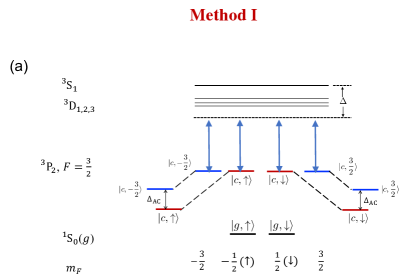
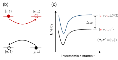
Figure 1: (color online) Schematic illustration of method I. (a): Single-atom energy levels and the $\pi$-polarized laser beam (blue lines with arrows). We also show the ³P₂ levels shifted by the beam. (b): A Two-atom spin-exchange process. The black (red) filled and dashed circles represent the $g(c)-$atom before and after a collision, respectively. Both this process and the inverse one are studied in this work. (c): The inter-atomic scattering channels. Here the solid curves represent the potentials of each channel. The coupling potentials between different channels are not shown in the figure.

II.1 AC-Stark Shifts and Heating Effects of ³P₂ States

As shown in Fig. 1(a), in our scheme a $\pi$-polarized laser beam is applied at a zero magnetic field, so that the ³P${}_{2}(F=3/2)$ states are far-off resonantly coupled to the excited states (e.g., the ³S₁ and ³D_1,2,3 states). Explicitly, all of the detunings of this beam with respect to the transition to the excited states 3pa are much larger than the fine splitting of these states. As a result, the energies of the ³P${}_{2}(F=3/2)$ states are shifted via the AC-Stark effect. We denote the ³P${}_{2}(F=3/2)$ states with $m_{F}=-1/2(+1/2)$ and $m_{F}=\pm 3/2$ as $|c,\uparrow\!(\downarrow)\rangle$ and $|c,\pm 3/2\rangle$, respectively. It is clear that AC-Stark shifts $E^{\rm(AC)}_{\xi}$of state $|c,\xi\rangle$ ($\xi=\uparrow,\downarrow,\pm 3/2$) satisfies

$$E^{\rm(AC)}_{\uparrow} = E^{\rm(AC)}_{\downarrow};\quad E^{\rm(AC)}_{-3/2}=E^{\rm(AC)}_{+3/2}.$$ (2)

We further define the difference between the AC-Stark shifts of states $|c,\uparrow\!(\downarrow)\rangle$ and $|c,\pm 3/2\rangle$ as (Fig. 1(a)):

$$\Delta_{\rm AC} \equiv E^{\rm(AC)}_{-3/2}-E^{\rm(AC)}_{\uparrow}.$$ (3)

Here we emphasize that, the spin-dependence of the AC-Stark effect for the ³P₂ levels of an alkaline-earth (like) atom is much more significant than the one of the electronic ground states of an ultracold alkali atom. As a result, to induce a given $\Delta_{\rm AC}$, the heating effect of the laser beams for our system is much lower than the ones for the alkali atoms.

This can be explained as follows. As mentioned before, here we consider the large-detuning cases where the detuning of the laser is much larger than the fine splitting of the electronic excited states. For the electronic ground manifold of an alkali atom, all the spin levels are in the same electronic orbit state, i.e., the S-state, and thus have the same dynamical polarizability. Therefore, the spin-dependence of the AC-Stark effect is essentially induced by the electronic spin-orbit coupling of the excited states Rudolf Grimm and Matthias Weidemüller and Yurii B. Ovchinnikov (1999); Hui Zhai (2021). Thus, to realize significant spin-dependence AC-Stark shifts in the large-detuning cases one has to apply an extremely strong beam, and thus the heating effect would be quite large. However, for an alkaline-earth (like) atom the electronic orbit states corresponding to the ³P₂ levels $|c,\xi\rangle$ ($\xi=\uparrow,\downarrow,\pm 3/2$) are different from each other. Precisely speaking, there are three electronic orbit P-states that are orthogonal with each other, and the level $|c,\xi\rangle$ corresponds to a $\xi$-dependent probability mixture of these three orbital states. As a result, these levels have different dynamical polarizability. Therefore, even in the large detuning cases, one can still realize very different AC-Stark shifts for these levels with weak laser beams, and thus the corresponding heating effects can be much weaker.

Figure 2: (color online) (a) The photon scattering rate $\Gamma_{\rm sc}$ of the system of method I, as a function of the AC-Stark shift difference $\Delta_{\rm AC}$, for the cases with detuning $\Delta$ of the laser beam with respect to the ³P₂-³S₁ transition (Fig. 1(a)) being $\Delta=(2\pi)1.3\times 10^{14}$Hz (green dotted line), $\Delta=(2\pi)2.3\times 10^{14}$Hz (blue dashed line) and $\Delta=(2\pi)3.3\times 10^{14}$Hz (red solid line). The laser wavelength corresponding to these cases is $1.15\mu$m, $1.89\mu$m, and $5.08\mu$m, respectively. (b) The ratio $\Gamma_{\rm sc}/\Delta_{\rm AC}$ as a function of $\Delta$ or the laser wavelength $\lambda_{\rm L}$.

The above discussions yield that for our system one can realize a very large AC-Stark shift difference $\Delta_{\rm AC}$ together with a long lifetime. To illustrate this, we calculate $\Delta_{\rm AC}$ and the photon scattering rate $\Gamma_{\rm sc}$ which describes the heating effect, for various cases. The details of this calculation are given in Appendix A.1, and the results are shown in Fig. 2. In the calculation we take into account the contributions from the excited states ³S₁ and ³D_1,2,3, which are mostly close to the ³P₂ levels. In Fig. 2(a) we illustrate $\Gamma_{\rm sc}$ as a function of $\Delta_{\rm AC}$ for the cases where the detuning $\Delta$ of the laser beams with respect to the ³P₂-³S₁ transition (Fig. 1(a)) takes various values. It is shown that for $\Delta=(2\pi)3.3\times 10^{14}$Hz (corresponding to laser wavelength 5.08$\mu$m) we have $\Gamma_{\rm sc}\sim$Hz when $\Delta_{\rm AC}\sim(2\pi)$MHz. If we estimate the lifetime of the ultracold gas as $1/\Gamma_{\rm sc}$, then this result yields that the lifetime of our system can be hundreds of milliseconds. In Fig. 2(b) we further show the ratio $\Gamma_{\rm sc}/\Delta_{\rm AC}$ as a function of $\Delta$ or the laser wavelength $\lambda_{\rm L}$. Since $\Gamma_{\rm sc}$ is always positive, the sign of this ratio is the same as the one of $\Delta_{\rm AC}$. In our scheme, $\Delta_{\rm AC}$ is required to be tuned to be positive. In addition, the divergence of $\Gamma_{\rm sc}/\Delta_{\rm AC}$ for $\Delta\approx(2\pi)1.85\times 10^{14}$Hz is because that we have $\Delta_{\rm AC}=0$ for this particular case. The divergences of $\Gamma_{\rm sc}/\Delta_{\rm AC}$ for the other four special values of $\Delta$ (including $\Delta=0$) shown in Fig. 2(b) are due to the resonance between the laser and the transitions from ³P₂ levels to the ³S₁ and ³D_1,2,3 states for these cases.

II.2 Effective Inter-Atomic Interaction

Our scheme is to control the effective SEI of two atoms in the states $|g,\uparrow\!(\downarrow)\rangle$ and $|c,\uparrow\!(\downarrow)\rangle$, respectively (Fig. 1(b)), with $|g\uparrow\!(\downarrow)$ being defined as the ¹S₀ states with $m_{F}=-1/2(+1/2)$. In this subsection, we derive the form of the effective interaction between these two atoms. To this end, we consider the $s$-wave scattering of these two atoms in the zero-energy limit, and perform discussions in the first-quantization formalism with the two atoms being labeled as 1 and 2. In the scattering process these two atoms are incident from the sub-space spanned by the following four states:

$$|g,\sigma;c,\sigma^{\prime}\rangle \equiv \frac{1}{\sqrt{2}}\left[|g,\sigma\rangle_{1}|c,\sigma^{\prime}\rangle_{2}-|c,\sigma^{\prime}\rangle_{1}|g,\sigma\rangle_{2}\right];$$ (4)

$$\hskip 93.89418pt(\sigma,\sigma^{\prime}=\uparrow,\downarrow).$$

Notice that since the atoms are identical fermions, the $s$-wave scattering occurs only when they are in anti-symmetric internal states. Furthermore, during the scattering process the inter-atomic interaction can couple the states in Eq. (4) to the states 4pa

$$|g,{\tilde{\sigma}};c,\xi\rangle \equiv \frac{1}{\sqrt{2}}\left[|g,{\tilde{\sigma}}\rangle_{1}|c,\xi\rangle_{2}-|c,\xi\rangle_{1}|g,{\tilde{\sigma}}\rangle_{2}\right],$$ (5)

$$\hskip 42.67912pt({\tilde{\sigma}}=\uparrow,\downarrow;\ \ \ \xi=\pm 3/2).$$

Taking into account these states, we can express Hamiltonian for the two-atom relative motion and internal states as

$${\hat{H}}=-\frac{\nabla^{2}_{\bf r}}{2\mu}+{\hat{H}}_{f}+{\hat{V}}^{(2)}({\bf r}),$$ (6)

where $\mu$ and ${\bf r}$ are the reduced mass and relative position of the two atoms, respectively, and ${\hat{V}}^{(2)}({\bf r})$ is the projection of the interaction potential between one atom in the ¹S₀ state and another atom in the ³P${}_{2}(F=3/2)$ states, respectively, on the subspace spanned by the states in Eqs. (4, 5). The explicit form of ${\hat{V}}^{(2)}({\bf r})$ is given in Appendix B. Moreover, in Eq. (6) the operator ${\hat{H}}_{f}$ is the free Hamiltonian of the internal state of the two atoms, which is given by

$${\hat{H}}_{f} = \Delta_{\rm AC}\!\!\sum_{\tiny\begin{array}[]{l}\sigma=\uparrow,\downarrow\\ \xi=\pm 3/2\end{array}}\!\!\!\!|g,\sigma;c,\xi\rangle\langle g,\sigma;c,\xi|$$ (9)

where the free energy of the states $|g,\sigma;c,\sigma^{\prime}\rangle$ ($\sigma,\sigma^{\prime}=\uparrow,\downarrow$) is chosen to be zero. Here we ignore the electronic ³P_0,1 and ³P₂ ($F=5/2$) states, because the energy differences between these states and the ones relevant to our proposal are very large.

In summary, there are four open channels (i.e., the channels corresponding to $|g,\sigma;c,\sigma^{\prime}\rangle$ with $\sigma,\sigma^{\prime}=\uparrow,\downarrow$) and four closed channels (i.e., the channels corresponding to $|g,\sigma;c,\xi\rangle$ with $\sigma=\uparrow,\downarrow$ and $\xi=\pm 3/2$) with the potential of each channel and the coupling between different channels all being determined by the interaction ${\hat{V}}^{(2)}({\bf r})$.

Furthermore, as shown in Appendix B, the interaction potential ${\hat{V}}^{(2)}({\bf r})$ is anisotropic, and can couple the wave functions with the angular momentum of two-atom relative motion being $l$ and $l+2$. Nevertheless, the projection

$$M\equiv m_{F1}+m_{F2}+m_{l}$$ (10)

of the total angular momentum along the $z$-axis is conserved in the scattering process, where $m_{F1,2}$ is the magnetic quantum number of the atoms 1,2, and $m_{l}$ is the $z$-component of the angular momentum of two-atom relative motion. Using this fact and other properties of ${\hat{V}}^{(2)}({\bf r})$ we find that in the zero-energy limit if the two atoms were incident from one of the following four states, i.e., the polarized states $|g,\uparrow;c,\uparrow\rangle$ and $|g,\downarrow;c,\downarrow\rangle$, and the anti-polarized states $|\pm\rangle$ defined by

$$|\pm\rangle\equiv\frac{1}{\sqrt{2}}\big{[}|g,\uparrow;c,\downarrow\rangle\mp|g,\downarrow;c,\uparrow\rangle\big{]},$$ (11)

then there is only elastic scattering, i.e., the two-atom internal state cannot be changed by the scattering process. We denote $|\Psi_{\sigma,\sigma}({\bf r})\rangle$ ($\sigma=\uparrow,\downarrow$) as the zero-energy scattering wave functions corresponding to the polarized incident state $|g,\sigma;c,\sigma\rangle$, and $|\Psi_{\pm}({\bf r})\rangle$ as the ones for the incident state $|\pm\rangle$ defined in Eq. (11). The above analysis yields

$$\lim_{r\rightarrow\infty}|\Psi_{+}({\bf r})\rangle = \left(1-\frac{a_{+}}{r}\right)|+\rangle;$$ (12)

$$\lim_{r\rightarrow\infty}|\Psi_{-}({\bf r})\rangle = \left(1-\frac{a_{-}}{r}\right)|-\rangle;$$ (13)

$$\lim_{r\rightarrow\infty}|\Psi_{\uparrow,\uparrow}({\bf r})\rangle = \left(1-\frac{a_{\rm f}}{r}\right)|g,\uparrow;c,\uparrow\rangle;$$ (14)

$$\lim_{r\rightarrow\infty}|\Psi_{\downarrow,\downarrow}({\bf r})\rangle = \left(1-\frac{a_{\rm f}}{r}\right)|g,\downarrow;c,\downarrow\rangle,$$ (15)

with $a_{\pm}$ and $a_{\rm f}$ being the corresponding elastic scattering lengths. Notice that the scattering lengths for the polarized incident states $|g,\uparrow;c,\uparrow\rangle$ and $|g,\downarrow;c,\downarrow\rangle$ are the same, because our system is invariant under the reflection with respect to the $x-y$ plane.

When the atoms are incident from a superposition of the four special states $|g,\uparrow;c,\uparrow\rangle$, $|g,\downarrow;c,\downarrow\rangle$ and $|\pm\rangle$, the scattering state would be the corresponding superposition of the ones in Eqs. (12-15), and thus the scattering amplitudes can be expressed in terms of $a_{\pm}$ and $a_{\rm f}$. In particular, when the atoms are incident from the anti-polarized state $|g,\downarrow;c,\uparrow\rangle$ or $|g,\uparrow;c,\downarrow\rangle$, the corresponding scattering wave function $|\Psi_{\downarrow,\uparrow}({\bf r})\rangle$ or $|\Psi_{\uparrow,\downarrow}({\bf r})\rangle$ satisfy

$$\lim_{r\rightarrow\infty}|\Psi_{\downarrow,\uparrow}({\bf r})\rangle = \left[1-\frac{(a_{-}+a_{+})/2}{r}\right]|g,\downarrow;c,\uparrow\rangle$$ (16)

$$-\frac{(a_{-}-a_{+})/2}{r}|g,\uparrow;c,\downarrow\rangle,$$

and

$$\lim_{r\rightarrow\infty}|\Psi_{\uparrow,\downarrow}({\bf r})\rangle = \left[1-\frac{(a_{-}+a_{+})/2}{r}\right]|g,\uparrow;c,\downarrow\rangle$$ (17)

$$-\frac{(a_{-}-a_{+})/2}{r}|g,\downarrow;c,\uparrow\rangle.$$

Eqs. (16, 17) yield that the spin-exchange scattering process

$$|g,\uparrow;c,\downarrow\rangle\Leftrightarrow|g,\downarrow;c,\uparrow\rangle$$ (18)

can occur, and the amplitude of spin-exchange is just $(a_{-}-a_{+})/2$.

According to the above discussion, the low-energy scattering between these two atoms can be described by the pseudo potential

$${\hat{V}}_{\rm eff}=\frac{2\pi}{\mu}\Big{[}a_{\rm+}|+\rangle\langle+|+a_{-}|-\rangle\langle-|+a_{\rm f}{\hat{P}}_{\rm f}\Big{]}\delta({\bf r})\frac{\partial}{\partial r}(r\cdot),$$

(19)

where

$${\hat{P}}_{\rm f}=\sum_{\sigma=\uparrow,\downarrow}|g,\sigma;c,\sigma\rangle\langle g,\sigma;c,\sigma|$$ (20)

is the projection operator of the polarized states.

In addition, we can treat the electronic states ¹S₀($g$) and ³P${}_{2}(F=3/2)$($c$) as the labels of the two atoms, and treat the $g$- and $c$-atoms as two distinguishable particles. Furthermore, both of these two atoms are particles with pseudo-spin $1/2$, because in the open channel each atom has two possible magnetic quantum numbers $\uparrow$ and $\downarrow$. In this treatment, one can express the effective two-atom Hamiltonian in the form mentioned in Sec. I, i.e.,

$$H_{\rm 2body}^{\rm(eff)}=\frac{{\bm{p}}_{S}^{2}}{2m}+\frac{{\bm{p}}_{P}^{2}}{2m}+{\hat{V}}_{\rm eff}.$$

Here ${\bm{p}}_{S(P)}$ is the momentum operator of the $g$- ($c$-) atom, and ${{\bm{p}}_{S}^{2}}/(2m)+{{\bm{p}}_{P}^{2}}/{(2m)}$ is the pseudo-spin independent free Hamiltonian, and

$${\hat{V}}_{\rm eff}=\frac{2\pi}{\mu}\times$$

$$\left[\!\frac{A_{x}}{2}\hat{\sigma}_{x}^{(S)}\hat{\sigma}_{x}^{(P)}\!+\!\frac{A_{y}}{2}\hat{\sigma}_{y}^{(S)}\hat{\sigma}_{y}^{(P)}\!+\!\frac{A_{z}}{2}\hat{\sigma}_{z}^{(S)}\hat{\sigma}_{z}^{(P)}\!+\!A_{0}\right]\!\delta({\bf r})\frac{\partial}{\partial r}(r\cdot)$$

(21)

is the effective inter-atomic interaction which is equivalent to the one of Eq (19). Here ${\hat{\sigma}}_{x,y,z}^{(S(P))}$ are the Pauli operators of the pseudo spin of the $g$-atom ($c$-atom), and the coefficients $A_{x,y,z,0}$ are given by

$$A_{x} = A_{y}$$ (22)

$$= \frac{a_{-}-a_{+}}{2};$$

$$A_{z} = \frac{2a_{\rm f}-(a_{-}+a_{+})}{2};$$ (23)

$$A_{0} = \frac{2a_{\rm f}+(a_{-}+a_{+})}{4}.$$ (24)

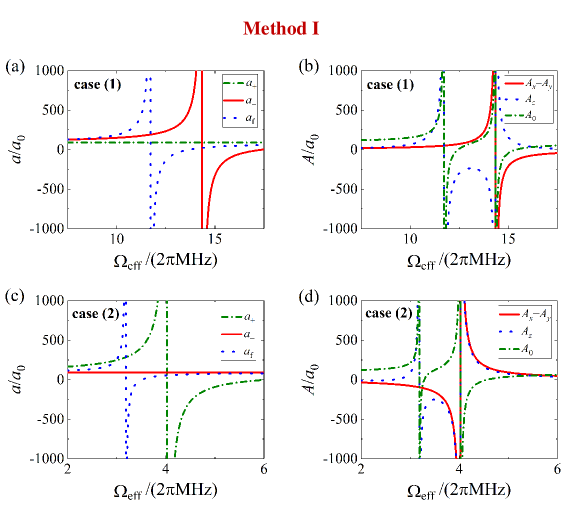
Figure 3: (color online) The scattering lengths $a_{\pm,{\rm f}}$ ((a), (c)) and interaction parameters $A_{x,y,z,0}$ ((b), (d)) of the system of method I. Here we show the results for two cases, which are given by the multi-channel square-well model in Sec. II.4, with width $b=85a_{0}$ and other parameters being given in Table I of Appendix C.

II.3 Resonant Control of $a_{\pm}$ and $a_{\rm f}$

Now we show that the scattering lengths $a_{\pm}$ and $a_{\rm f}$ can be resonantly controlled by the AC-Stark shift difference $\Delta_{\rm AC}$.

As mentioned above, the open channels corresponding to $|g,\sigma;c,\sigma^{\prime}\rangle$ ($\sigma,\sigma^{\prime}=\uparrow,\downarrow$) is coupled to the closed channels corresponding to $|g,\sigma;c,\xi\rangle$ ($\sigma=\uparrow,\downarrow$ and $\xi=\pm 3/2$) by the anisotropic interaction ${\hat{V}}^{(2)}({\bf r})$. Explicitly, due to the conservation of the angular momentum $M$ defined in Eq. (10), the $s$-wave states of the open channels of our system are coupled to the $d$-wave states of the closed channels. Therefore, the scattering lengths $a_{\pm,{\rm f}}$ depend on the energy gaps between the thresholds of the open and closed channels, which is just the AC-Stark shift $\Delta_{\rm AC}$ (Fig. 1(c)), and thus one can control these scattering lengths through $\Delta_{\rm AC}$ by changing the intensities of the laser beam.

Furthermore, as shown before, the order of magnitude of $\Delta_{\rm AC}$ can be as large as $(2\pi)$MHz, with the photon scattering rate $\Gamma_{\rm sc}$ being only of the order of Hz. On the other hand, the characteristic energy corresponding to the length scale of the inter-atomic van der Waals interaction potential, i.e., the van der Waals energy $E_{\rm vdW}$, is also of this order for Yb atoms one . Therefore, if the closed channels have $d$-wave bound states with binding energy $|E_{\uparrow}|$ comparable or less than $E_{\rm vdW}$, by tuning $\Delta_{\rm AC}$ via the laser intensity one can make the open channels to be near-resonant to the closed-channel bound states, i.e., realize Feshbach resonances, while keeping the heating effect being low enough. At each resonance point, one of the three scattering lengths $a_{\pm,{\rm f}}$ diverges. Around the resonances, one can efficiently manipulate $a_{\pm,{\rm f}}$ (or the interaction parameters $A_{x,y,z,0}$). That is the basic principle of this method.

II.4 Illustration with Multi-Channel Square-Well Model

We illustrate our approach with a calculation for the scattering lengths $a_{\pm,{\rm f}}$ and the interaction parameters $A_{x,y,z,0}$ defined above. As shown in Appendix B, the potential ${\hat{V}}^{(2)}({\bf r})$ can be expressed as

$${\hat{V}}^{(2)}({\bf r})=\sum_{\eta=1}^{6}V^{(2)}_{\eta}(r){\hat{D}}_{\eta}({\hat{\bf r}}),$$ (25)

where $r=|{\bf r}|$ and ${\hat{\bf r}}={\bf r}/r$. Here $V^{(2)}_{1,...,6}(r)$ are the potential curves corresponding to six different electronic states. These electronic states are defined in Appendix B, together with the operators ${\hat{D}}_{1,...,6}({\hat{\bf r}})$. As mentioned before, we do not know the parameters of the potential curves $V^{(2)}_{1,...,6}(r)$. Therefore, we can only qualitatively illustrate our proposal with a multi-channel square-well model with

$$V^{(2)}_{\eta}(r)=-U^{(2)}_{\eta}\theta(b-r),\ \ \ (r\geq 0;\ \eta=1,...,6),$$ (26)

where $\theta(x)$ is the step function satisfying $\theta(x)=1$ for $x\geq 0$ and $\theta(x)=0$ for $x<0$. In our calculation, we choose $b=85a_{0}$, with $a_{0}$ being the Bohr radius and $2b$ taking a typical value of the length scale $\beta_{6}$ associated with the van der Waals interaction between atoms as heavy as Ytterbium two . We consider all the involved $s$-wave and $d$-wave channels, and ignore the channels with higher relative angular momentum, for simplicity. We also ignore the centrifugal potential of the $d$-wave channels in the region $r<d$ because the square-well potentials in this region are very deep.

We display the results for two cases in Fig. 3. In Table I of Appendix C we show the value of the potential depth $U^{(2)}_{\eta}$ $(\eta=1,...,6)$ as well as the $s$-wave scattering length $a_{\eta}^{(2)}$ corresponding to a single-channel square-well potential $V^{(2)}_{\eta}(r)$ given in Eq. (26). In Fig. 3 we illustrate the behaviors of both the scattering lengths $a_{\pm,{\rm f}}$ and the interaction parameters $A_{x,y,z,0}$ defined in Eqs. (22-24) as functions of $\Delta_{\rm AC}$. It is shown that using the resonances one can tune the intensity $A_{x}=A_{y}$ of the effective SEI as well as the intensities $A_{z,0}$ of the spin-non-exchanging and spin-independent interaction in a broad region e.g., between $-1000a_{0}$ and $1000a_{0}$ through the laser intensity, and may prepare the effective inter-atomic interaction ${\hat{V}}_{\rm eff}$ to be either “anti-ferromagnetic like” ($A_{x}=A_{y}>{\rm Max}[0,-A_{z}]$) with the lowest eigen state being the singlet state $|+\rangle$ defined in Eq. (11), or “ferromagnetic like” ($A_{z}<0$ and $|A_{x}|=|A_{y}|<|A_{z}|$) with the lowest eigen states being the polarized ones $|g,\uparrow;c,\uparrow\rangle$ and $|g,\downarrow;c,\downarrow\rangle$. It is also possible to “turn off” the spin-independent interaction by tuning $A_{0}=0$ or prepare the system to other required interaction parameter regions. In Appendix D we show the values of $\Delta_{\rm AC}$ under which we have $A_{0}=0$ for the two cases in Fig. 3, as well as the corresponding values of $A_{x,y,z}$ and the scattering lengths $a_{\pm,f}$.

III Method II

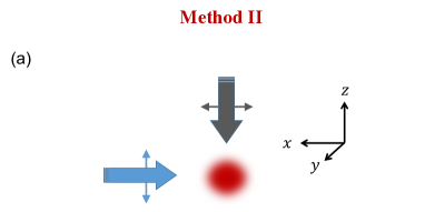
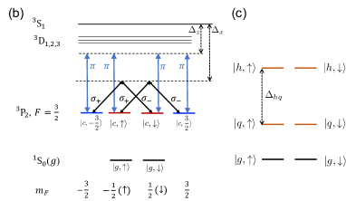
Figure 4: (color online) Schematic illustration for method II. (a): Two laser beams polarized along the $z$-direction and the $x$-direction, respectively, are applied to the atoms. (b): 1-atom bare levels as well as the influences of the laser beams. Here the beam polarized along the $x$-direction is decomposed into two beams with $\sigma_{+}$ and $\sigma_{-}$ polarizations, respectively. (c): 1-atom dressed levels in the rotating frame. (d): A 2-atom spin-exchange process. The black (red) filled and dashed circles represent the $g(q)-$atom before and after a collision, respectively. Both this process and the inverse one are studied in this work. (e):The inter-atomic scattering channels. Here the solid curves represent the potentials of each channel. The coupling potentials between different channels are not shown in the figure.

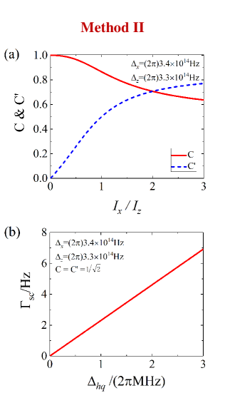
Figure 5: (color online) (a): The parameters $C$ and $C^{\prime}$ in Eqs. (27-30) as a function of $I_{x}/I_{z}$, with $I_{z(x)}$ being the intensity of the laser beam polarized along the $z$-($x$-)direction. Here we show the results for the cases with $\Delta_{z}=(2\pi)3.3\times 10^{14}$Hz and $\Delta_{x}=(2\pi)3.4\times 10^{14}$Hz, where $\Delta_{z(x)}$ is the detuning of the $z(x)$-polarized laser beam with respect to the ³P₂-³S₁ transition (Fig. 4(a)). In this case the wave length of the $z(x)$-polarized laser beam is $5.08\mu$m ($6.12\mu$m). (b): The total photon scattering rate $\Gamma_{\rm sc}$ as a function of the energy gap $\Delta_{hq}$ between the higher dressed states $|h,\uparrow\!(\downarrow)\rangle$ and the lower dressed states $|q,\uparrow\!(\downarrow)\rangle$. Here we show the results for the cases with $C^{\prime}=C=1/\sqrt{2}$, and the frequencies of the laser beams polarized along the $z$- ($x$-) direction being the same as (a).

Now we introduce our second approach for the manipulation of SEI. As above, we also take the system of two ¹⁷¹Yb atoms as an example. In addition, to avoid using too many different symbols, in this and the next section, we will use some notations which have already been used in Sec. II, for the clear-enough cases (e.g., we still use $\Gamma_{\rm sc}$ to denote the photon scattering rate of laser beams for the current scheme). The exact definitions of these notations for this section will all be given in the following discussions.

Figure 6: (color online) The scattering lengths $a_{\pm}$ and $p_{\pm}$ ((a), (c)) and interaction parameters $A_{x,y,z,0}$ ((b), (d)) of the system of method II. Here we show the results for two cases, which are given by the multi-channel square-well model in Sec. II.4, with width $b=85a_{0}$ and other parameters being given in Table II of Appendix C. The values of $\Delta_{hq}$ under which we have $A_{0}=0$, as well as the corresponding values of $A_{x,y,z}$ and $a_{\pm,p\pm}$, are shown in Appendix D.

Method II is a generalization of method I. In this approach two laser beams are applied, which are polarized along the $z$-direction and the the $x$-direction, respectively (Fig. 4(a)). Both of these two beams are far-off resonant for the transition from the ³P${}_{2}(F=3/2)$ level to the excited states (i.e., the detunings are much larger than the Rabi frequencies of the transitions and the natural linewidth of the excited states), similar as in Sec. II. The frequency difference of these two beams is not required to take any certain value. The only requirement for this frequency difference is that it should be much larger than the AC-Stark shifts induced by each beam so that the two beams induce the second-order effects for the ³P${}_{2}(F=3/2)$ level independently. In this case, the total effect of these two beams is not equivalent to the one of a single beam polarized along some direction between the $x$- and $z$-axis.

As in Sec. II.1, the beam polarized along the $z$-direction can induce spin-dependent AC-Stark shifts for the states in the ³P${}_{2}(F=3/2)$ level. Meanwhile, the beam polarized along the $x$-direction can be decomposed into two beams with $\sigma_{+}$ and $\sigma_{-}$ polarizations, respectively, and thus induces Raman coupling between the ³P${}_{2}(F=3/2)$ state with $m_{F}=-3/2(+3/2)$ and the one with $m_{F}=1/2(-1/2)$ (Fig. 4(b)). As a result, four dressed states $|q(h),\uparrow\!(\downarrow)\rangle$ can be formed (Fig. 4(c)), which can be expressed as

$$|h,\uparrow\rangle = C^{\prime}|c,\uparrow\rangle+C|c,3/2\rangle,$$ (27)

$$|q,\uparrow\rangle = -C|c,\uparrow\rangle+C^{\prime}|c,3/2\rangle;$$ (28)

and

$$|h,\downarrow\rangle = C^{\prime}|c,\downarrow\rangle+C|c,-3/2\rangle,$$ (29)

$$|q,\downarrow\rangle = -C|c,\downarrow\rangle+C^{\prime}|c,-3/2\rangle;$$ (30)

where $|c,\sigma\rangle$ ($\sigma=\uparrow,\downarrow,\pm 3/2$) are just the ³P${}_{2}(F=3/2)$ states, as defined in Sec. II and shown in (Fig. 4(b)). The coefficients $C$ and $C^{\prime}$ in Eqs. (27-30), are determined by the intensities and frequencies of the two laser beams, with the expressions being derived in Appendix A.2. In Fig. 5(a) we show the values of $C$ and $C^{\prime}$ as functions of the ratio between the intensities of the two laser beams for typical cases. Furthermore, due to the reflection symmetry with respect to the $x-y$ plane, the two lower (higher) dressed states $|q(h),\uparrow\rangle$ and $|q(h),\downarrow\rangle$ are degenerate (Fig. 4(c)). The energy gap $\Delta_{hq}$ between these higher and lower dressed states (Fig. 4(c)) is also derived in Appendix A.2, where we find that $\Delta_{hq}$ can be expressed as

$$\Delta_{hq}=\sqrt{\left[\Delta_{\rm AC}^{(z)}-\Delta_{\rm AC}^{(x)}/2\right]^{2}+\frac{3}{4}\Delta_{\rm AC}^{(x)2}},$$ (31)

where $\Delta_{\rm AC}^{(z(x))}$ is the AC-Stark shift difference only induced by the laser beams polarized along the $z$- ($x$-) direction, as defined in Sec. II. Therefore, $\Delta_{hq}$ has the same order of magnitude with the AC-Stark shift difference $\Delta_{\rm AC}^{(z(x))}$, as mentioned in Sec. I.

Furthermore, the total photon scattering rate $\Gamma_{\rm sc}$ of these two beams, which describes the heating effects, can also be calculated directly (Appendix A.2). In Fig. 5(b) we show $\Gamma_{\rm sc}$ as a function of $\Delta_{hq}$ for a typical case. It is shown that we have $\Gamma_{\rm sc}\sim$Hz when $\Delta_{hq}\sim(2\pi)$MHz. Therefore, the laser-induced heating effect is weak, which is similar to the one in Sec. II.

Furthermore, similar as in Sec. II, our method is to control the SEI between two atoms in the ¹S₀ state ($g$-state) and the lower dressed state ($q$-state) (Fig. 4(d)). To this end, we consider the scattering processes in the zero-energy limit, with incident states being in the Hilbert space spanned by the states:

$$|g,\sigma;q,\sigma^{\prime}\rangle \equiv \frac{1}{\sqrt{2}}\left[|g,\sigma\rangle_{1}|q,\sigma^{\prime}\rangle_{2}-|q,\sigma^{\prime}\rangle_{1}|g,\sigma\rangle_{2}\right];$$ (32)

$$\hskip 93.89418pt(\sigma,\sigma^{\prime}=\uparrow,\downarrow).$$

In addition, the inter-atomic interaction $V^{(2)}({\bf r})$ couples these open channels corresponding to the above four states to the closed channels corresponding to

$$|g,\sigma;h,\sigma^{\prime}\rangle \equiv \frac{1}{\sqrt{2}}\left[|g,\sigma\rangle_{1}|h,\sigma^{\prime}\rangle_{2}-|h,\sigma^{\prime}\rangle_{1}|g,\sigma\rangle_{2}\right],$$ (33)

$$\hskip 93.89418pt(\sigma,\sigma^{\prime}=\uparrow,\downarrow;).$$

The energy gap between the above open and closed channels is just $\Delta_{hp}$, as shown in Fig. 4(e).

In addition, using an analysis based on the properties of the interaction potential ${\hat{V}}^{(2)}({\bf r})$, which is similar to the discussion in Sec. II.2, we find that in the zero-energy limit if the two atoms were incident from one of the following four states:

$$|\pm\rangle \equiv \frac{1}{\sqrt{2}}\big{[}|g,\uparrow;q,\downarrow\rangle\mp|g,\downarrow;q,\uparrow\rangle\big{]};$$ (34)

$$|p_{\pm}\rangle \equiv \frac{1}{\sqrt{2}}\big{[}|g,\uparrow;q,\uparrow\rangle\mp|g,\downarrow;q,\downarrow\rangle\big{]},$$ (35)

then in the zero-energy limit there are only elastic scattering processes in which the two-atom internal state is not changed. We denote the elastic scattering lengths with respect to the incident states $|\pm\rangle$ and $|p_{\pm}\rangle$ as $a_{\pm}$ and $a_{p\pm}$, respectively. Notice that for the current system it is possible that $a_{p+}\neq a_{p-}$, i.e., the spin-change processes $|g,\uparrow,q;\uparrow\rangle\Leftrightarrow|g,\downarrow;q,\downarrow\rangle$ are also permitted. Therefore, the low-energy interaction between these two atoms can be described by the pseudo potential

$${\hat{V}}_{\rm eff}=\frac{2\pi}{\mu} \Big{[}a_{\rm+}|+\rangle\langle+|+a_{-}|-\rangle\langle-|$$

$$+a_{p+}|p_{+}\rangle\langle p_{+}|+a_{p-}|p_{-}\rangle\langle p_{-}|\Big{]}\delta({\bf r})\frac{\partial}{\partial r}(r\cdot).$$

Moreover, by treating the atoms in $|g,\uparrow\!(\downarrow)\rangle$ and $|q,\uparrow\!(\downarrow)\rangle$ as two distinguished particles with pseudo-spin $1/2$, one can express the effective two-atom Hamiltonian in the form of Sec. I, i.e.,

$$H_{\rm 2body}^{\rm(eff)}=\frac{{\bm{p}}_{S}^{2}}{2m}+\frac{{\bm{p}}_{P}^{2}}{2m}+{\hat{V}}_{\rm eff}.$$

Here ${\bm{p}}_{S(P)}$ is the momentum operator of the $g$- ($q$-) atom and ${{\bm{p}}_{S}^{2}}/(2m)+{{\bm{p}}_{P}^{2}}/{(2m)}$ is the pseudo-spin independent free Hamiltonian, and the effective inter-atomic interaction

$${\hat{V}}_{\rm eff}=\frac{2\pi}{\mu}\times$$

$$\left[\!\frac{A_{x}}{2}\hat{\sigma}_{x}^{(S)}\hat{\sigma}_{x}^{(P)}\!+\!\frac{A_{y}}{2}\hat{\sigma}_{y}^{(S)}\hat{\sigma}_{y}^{(P)}\!+\!\frac{A_{z}}{2}\hat{\sigma}_{z}^{(S)}\hat{\sigma}_{z}^{(P)}\!+\!A_{0}\right]\!\delta({\bf r})\frac{\partial}{\partial r}(r\cdot)$$

(37)

is equivalent to the one of Eq. (LABEL:veff2), with ${\hat{\sigma}}_{x,y,z}^{(S(P))}$ being the Pauli operators of the pseudo spin of the $g$- ($q$-) atom. In Eq. (37) the coefficients $A_{x,y,z,0}$ are related to the scattering lengths $a_{\pm}$ and $a_{p\pm}$ via

$$A_{x} = \frac{(a_{-}-a_{+})+(a_{p-}-a_{p+})}{2};$$ (38)

$$A_{y} = \frac{(a_{-}-a_{+})-(a_{p-}-a_{p+})}{2};$$ (39)

$$A_{z} = \frac{(a_{p-}+a_{p+})-(a_{-}+a_{+})}{2};$$ (40)

$$A_{0} = \frac{(a_{p-}+a_{p+})+(a_{-}+a_{+})}{4}.$$ (41)

Notice that in the current system the interaction parameters $A_{x}$ and $A_{y}$ may be unequal.

Similar to before, by changing the intensities of the two laser beams, one can tune the energy gap $\Delta_{hp}$ and induce Feshbach resonances. The scattering lengths $a_{\pm}$ and $a_{p\pm}$ or the interaction parameters $A_{x,y,z,0}$ can be efficiently manipulated via these Feshbach resonances. We illustrate these resonances via the multi-channel square-well model used in Sec. II.4, with width $b=85a_{0}$ and other parameters being given in Table II of Appendix C. The results are shown in Fig. 6.

We emphasis that there is an important difference between the current approach and method I. For the system of method I, the $s$-wave states of the open channels are coupled only to the $d$-wave states of the closed channels, as mentioned in the above sections. However, for our current system, the $s$-wave open-channel states are coupled to both the $d$-wave and the $s$-wave states of the closed channels. As discussed in Sec. I, this fact implies that the Feshbach resonances for $a_{\pm}$ with a low-enough heating rate are much more possible to appear for realistic systems. That is an important advantage of the current method.

IV Method III

Now we introduce our third approach for the manipulation of SEI, which is based on the ³P₂-³P₀ Raman coupling, by taking ¹⁷¹Yb atoms as an example. As before, we will use some notations which have been used in Sec. II, to reduce the number of different symbols. The exact definitions of these notations for this section will be given below.

IV.1 Low-Heating Raman Coupling between ³P₀ and ³P₂ Levels

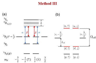
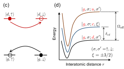
Figure 7: (color online) Schematic illustration of method III. (a): 1-atom bare levels and $\pi$-polarized Raman beams (blue and red lines). Here $\Delta$ is the single-photon detuning. (b): 1-atom dressed levels in the rotating frame. (c): A 2-atom spin-exchange process. The black (red) filled and dashed circles represent the $g(d)-$atom before and after a collision, respectively. Both this process and the inverse one are studied in this work. (d):The inter-atomic scattering channels. Here the solid curves represent the potentials of each channel. The coupling potentials between different channels are not shown in the figure.

As shown in Fig. 7(a), in the current method two $\pi$-polarized laser beams $\alpha$ and $\beta$ are applied at a zero magnetic field so that the ³P_0,2 levels are far-off resonantly coupled to the excited states. These two beams can induce a Raman coupling between the states $|^{3}{\rm P}_{0},1/2,\sigma\rangle$ and $|^{3}{\rm P}_{2},3/2,\sigma\rangle$, with $\sigma=-1/2(\uparrow)$ or $1/2(\downarrow)$. Furthermore, the frequency difference of these two beams is tuned to compensate for the difference of the AC-Stark shifts of these states, so that this Raman coupling is resonant. Explicitly, the fluctuation of this frequency difference should be much less than the effective Rabi frequency $\Omega_{\rm eff}$ of the Raman coupling, which is of the order of $(2\pi)$MHz as shown below.

As a result of this resonant Raman coupling, the eigen states of the single-atom Hamiltonian $H_{\rm 1b}$ in the rotating frame are given by (Appendix A.3):

$$|d,\sigma\rangle \equiv \frac{1}{\sqrt{2}}\left[|^{3}{\rm P}_{0},1/2,\sigma\rangle-|^{3}{\rm P}_{2},3/2,\sigma\rangle\right];$$ (42)

$$|u,\sigma\rangle \equiv \frac{1}{\sqrt{2}}\left[|^{3}{\rm P}_{0},1/2,\sigma\rangle+|^{3}{\rm P}_{2},3/2,\sigma\rangle\right];$$ (43)

$$|g,\sigma\rangle \equiv |^{1}{\rm S}_{0},1/2,\sigma\rangle;$$ (44)

$$|c,\xi\rangle \equiv |^{3}{\rm P}_{2},3/2,\xi\rangle,$$

$$(\sigma=\uparrow,\downarrow,\xi=\pm 3/2).$$

where the states $|g,\sigma\rangle$ and $|c,\xi\rangle$ ($\sigma=\uparrow,\downarrow,\xi=\pm 3/2$) have the same definitions as in the above two sections. In addition, the eigen energies of $H_{\rm 1b}$ corresponding to the states in Eqs. (42,43,44,IV.1) can be denoted as ${\cal E}_{d}$, ${\cal E}_{u}$, ${\cal E}_{g}$ and ${\cal E}_{c}$, respectively, and are all independent of the values of $\sigma$ or $\xi$. Namely, these eigen states are two-fold degenerate. Moreover, the energy gaps between the states $|d,\sigma\rangle$, $|u,\sigma\rangle$, and $|c,\xi\rangle$ $(\sigma=\uparrow,\downarrow,\xi=\pm 3/2)$ are (Appendix A.3, Fig. 7(b)):

$${\cal E}_{u}-{\cal E}_{d} = \Omega_{\rm eff};$$ (46)

$${\cal E}_{c}-{\cal E}_{d} = E^{\rm(AC)}_{-3/2}-E^{\rm(AC)}_{\uparrow}+\Omega_{\rm eff}/2\equiv\delta_{cd},$$ (47)

where $\Omega_{\rm eff}>0$ is the Rabi frequency of the Raman coupling and $E^{\rm(AC)}_{\zeta}$ ($\zeta=\downarrow,3/2$) is the AC-Stark shift of the state $|^{3}{\rm P}_{2},3/2,\zeta\rangle$, which can be controlled by the intensities of the Raman beams. Our current scheme works in the region with $\delta_{cd}>0$.

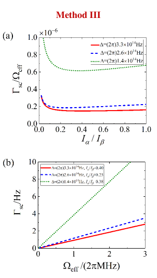
Figure 8: (color online) (a) The ratio between the photon scattering rate $\Gamma_{\rm sc}$ and the effective Rabi frequency $\Omega_{\rm eff}$ of the system of method III, as a function of the laser intensity ratio $I_{\alpha}/I_{\beta}$ for the cases where the one-photon detuning $\Delta$ the Raman beams with respect to the ³S₁ state (Fig. 7(a)) takes the values $\Delta=(2\pi)3.3\times 10^{14}$Hz (red solid line), $\Delta=(2\pi)2.6\times 10^{14}$Hz (blue dashed line), and $\Delta=(2\pi)1.4\times 10^{14}$Hz (green dotted line). (b) $\Gamma_{\rm sc}$ as a function of $\Omega_{\rm eff}$ for the cases of (a). For each $\Delta$ the laser intensity ratio $I_{\alpha}/I_{\beta}$ takes the value to minimize $\Gamma_{\rm sc}/\Omega_{\rm eff}$.

Furthermore, this ${}^{3}{\rm P}_{2}$-${}^{3}{\rm P}_{0}$ Raman coupling is much stronger than the Raman coupling between different hyperfine states of an ultracold alkali atom, or equivalently, the heating effect for our system is much lower than the one for the alkali atoms. This can be understood with the following analysis. As in Sec. II.1 and Sec. III, our current method works in the large-detuning cases where the detuning of the one-photon transition induced by each Raman laser is much larger than the fine splitting of the corresponding excited state. For an alkali atom in the electronic ground state, the two hyperfine levels coupled by the Raman beams are in orthogonal atomic spin states. As a result, this Raman coupling cannot be created only by the laser-induced electric dipole transition (EDT). It is essentially led by both the EDT and the spin-orbit coupling of the atomic excited states. Thus, the Raman coupling is very weak for the large-detuning cases. However, for our system, the ${}^{3}{\rm P}_{0}$ and ${}^{3}{\rm P}_{2}$ states coupled by the Raman beams have a non-zero probability to be in the same state of electronic and nuclear spin. Therefore, the Raman effect can be induced only by EDT. Thus, one can obtain strong Raman coupling in the large-detuning cases.

Explicitly, for our system the ratio $\Gamma_{\rm sc}/\Omega_{\rm eff}$ between the photon scattering rate $\Gamma_{\rm sc}$ and the effective Rabi frequency $\Omega_{\rm eff}$ of the Raman coupling is a function of $\Delta$ and $I_{\alpha}/I_{\beta}$, where $\Delta$ is the one-photon detuning the Raman beams with respect to the ³S₁ state (Fig. 7(a)), and $I_{\alpha,\beta}$ are the intensities of the two Raman beams $\alpha$ and $\beta$ (we denote $\alpha$ as the beam with higher frequency, as shown in Fig. 7(a)). In Fig. 8(a) we illustrate the variation of $\Gamma_{\rm sc}/\Omega_{\rm eff}$ with $I_{\alpha}/I_{\beta}$, for various $\Delta$, which are calculated in Appendix A.3. It is shown that for a fixed $\Delta$ the ratio $\Gamma_{\rm sc}/\Omega_{\rm eff}$ can be minimized when $I_{\alpha}/I_{\beta}$ is tuned to a particular value. In Fig. 8(b) we further show $\Gamma_{\rm sc}$ as a function of $\Omega_{\rm eff}$, with $I_{\alpha}/I_{\beta}$ taking the value to minimize $\Gamma_{\rm sc}/\Omega_{\rm eff}$. It is shown that when $\Delta$ is as large as $(2\pi)3.3\times 10^{14}$Hz, one can realize a Raman coupling with $\Omega_{\rm eff}$ being several $(2\pi)$MHz, while the photon scattering rate $\Gamma_{\rm sc}$ is still of the order of Hz.

IV.2 Effective Inter-Atomic Interaction

Our current scheme is to control the SEI of two atoms being in the ¹S₀ state and the lower ³P dressed state ($d$-state), respectively, as shown in Fig. 7(c). Now we derive the effective interaction between these two atoms. Since the analysis is very similar to the one of Sec. II.2, here we only show the main results.

We consider the $s$-wave scattering of these two atoms in the zero-energy limit, which is at a zero magnetic field. For this scattering process, there are the following open channels:

$$|g,\sigma;d,\sigma^{\prime}\rangle \equiv \frac{1}{\sqrt{2}}\left[|g,\sigma\rangle_{1}|d,\sigma^{\prime}\rangle_{2}-|d,\sigma^{\prime}\rangle_{1}|g,\sigma\rangle_{2}\right],$$ (48)

$$\hskip 85.35826pt(\sigma,\sigma^{\prime}=\uparrow,\downarrow),$$

as well as the closed channels:

$$|g,\sigma;u,\sigma^{\prime}\rangle \equiv \frac{1}{\sqrt{2}}\left[|g,\sigma\rangle_{1}|u,\sigma^{\prime}\rangle_{2}-|u,\sigma^{\prime}\rangle_{1}|g,\sigma\rangle_{2}\right];$$ (49)

$$|g,\sigma;c,\xi\rangle \equiv \frac{1}{\sqrt{2}}\left[|g,\sigma\rangle_{1}|c,\xi\rangle_{2}-|c,\xi\rangle_{1}|g,\sigma\rangle_{2}\right],$$ (50)

$$(\sigma,\sigma^{\prime}=\uparrow,\downarrow;\ \ \ \xi=\pm 3/2).$$

The energy gap between the open channel and the closed channels in Eq. (49) and Eq. (50) are $\Omega_{\rm eff}$ and $\delta_{cd}$, respectively, as shown in Fig. 7(d). In addition, for our system, the inter-atomic interaction ${\hat{V}}({\bf r})$ can be expressed as

$${\hat{V}}({\bf r})={\hat{V}}^{(0)}(r)+{\hat{V}}^{(2)}({\bf r}),$$ (51)

where ${\hat{V}}^{(0(2))}(r)$ is the interaction between two atoms in the ¹S₀ and ³P₀ (³P${}_{2}(F=3/2)$) states, respectively, with the explicit forms being given in Appendix B.

Figure 9: (color online) The scattering lengths $a_{\pm,{\rm f}}$ ((a), (c)) and interaction parameters $A_{x,y,z,0}$ ((b), (d)) of the system of method III. Here we show the results for two cases, which are given by the multi-channel square-well model in Sec. II.4, with width $b=81a_{0}$ and other parameters being given in Table III of Appendix C. The values of $\Omega_{\rm eff}$ under which we have $A_{0}=0$, as well as the corresponding values of $A_{x,y,z}$ and $a_{\pm,f}$, are shown in Appendix D.

As in Sec. II.2, a straightforward analysis based on the form of ${\hat{V}}({\bf r})$ (Appendix B) shows that in the zero-energy limit if the two atoms were incident from one of the following four states, i.e., the polarized states $|g,\uparrow;d,\uparrow\rangle$ and $|g,\downarrow;d,\downarrow\rangle$ as well as the states $|\pm\rangle$ defined by

$$|\pm\rangle\equiv\frac{1}{\sqrt{2}}\big{[}|g,\uparrow;d,\downarrow\rangle\mp|g,\downarrow;d,\uparrow\rangle\big{]},$$ (52)

then the output state of the scattering process would be exactly the same as the incident state, i.e., there is only elastic scattering. We denote the scattering lengths corresponding to the incident states $|\pm\rangle$ as $a_{\pm}$. In addition, due to the reflection symmetry with respect to the $x-y$ plane, the scattering lengths corresponding to the incident states $|g,\uparrow;d,\uparrow\rangle$ and $|g,\downarrow;d,\downarrow\rangle$ are the same, and can be denoted as $a_{\rm f}$. Thus, the amplitude for the spin-exchange process $|g,\uparrow;d,\downarrow\rangle\Leftrightarrow|g,\downarrow;d,\uparrow\rangle$ is just $(a_{-}-a_{+})/2$.

Therefore, the low-energy interaction between these two atoms can be described by the pseudo potential

$${\hat{V}}_{\rm eff}=\frac{2\pi}{\mu}\Big{[}a_{\rm+}|+\rangle\langle+|+a_{-}|-\rangle\langle-|+a_{\rm f}{\hat{P}}_{\rm f}\Big{]}\delta({\bf r})\frac{\partial}{\partial r}(r\cdot),$$

(53)

where

$${\hat{P}}_{\rm f}=\sum_{\sigma=\uparrow,\downarrow}|g,\sigma;d,\sigma\rangle\langle g,\sigma;d,\sigma|$$ (54)

is the projection operator of the polarized states. As in the above sections, we can treat the atoms in $|g,\uparrow\!(\downarrow)\rangle$ and $|d,\uparrow(\downarrow)\rangle$ as two distinguished particles with pseudo-spin $1/2$, and express the effective two-atom Hamiltonian as

$$H_{\rm 2body}^{\rm(eff)}=\frac{{\bm{p}}_{S}^{2}}{2m}+\frac{{\bm{p}}_{P}^{2}}{2m}+{\hat{V}}_{\rm eff},$$

with ${\bm{p}}_{S(P)}$ being the momentum operator of the $g$- ($d$-) atom and ${{\bm{p}}_{S}^{2}}/(2m)+{{\bm{p}}_{P}^{2}}/{(2m)}$ being the pseudo-spin independent free Hamiltonian, and

$${\hat{V}}_{\rm eff}=\frac{2\pi}{\mu}\times$$

$$\left[\!\frac{A_{x}}{2}\hat{\sigma}_{x}^{(S)}\hat{\sigma}_{x}^{(P)}\!+\!\frac{A_{y}}{2}\hat{\sigma}_{y}^{(S)}\hat{\sigma}_{y}^{(P)}\!+\!\frac{A_{z}}{2}\hat{\sigma}_{z}^{(S)}\hat{\sigma}_{z}^{(P)}\!+\!A_{0}\right]\!\delta({\bf r})\frac{\partial}{\partial r}(r\cdot)$$

(55)

is the effective inter-atomic interaction, which is equivalent to the one of Eq. (53). For the current system, ${\hat{\sigma}}_{\pm}^{(j)}=({\hat{\sigma}}_{x}^{(j)}\pm i{\hat{\sigma}}_{y}^{(j)})/2$ ($j=S,P$), and ${\hat{\sigma}}_{x,y,z}^{(S(P))}$ are the Pauli operators of the pseudo spin of the $g$-atom ($d$-atom). In addition, the relation between coefficients $A_{x,y,z,0}$ and the scattering lengths $a_{\pm,{\rm f}}$ are same as Eqs. (22-24), i.e.,

$$A_{x} = A_{y}$$ (56)

$$= \frac{a_{-}-a_{+}}{2};$$

$$A_{z} = \frac{2a_{\rm f}-(a_{-}+a_{+})}{2};$$ (57)

$$A_{0} = \frac{2a_{\rm f}+(a_{-}+a_{+})}{4}.$$ (58)

IV.3 Resonant Control of ${\hat{V}}_{\rm eff}$

Due to the conservation of the angular momentum component $M$ defined in Eq. (10), the $s$-wave states of open channels of our system are coupled to both the $s$-wave and the $d$-wave states of the closed channels by the interaction ${\hat{V}}({\bf r})$. Furthermore, the energy gap $\delta_{cd}$ ($\Omega_{\rm eff}$) between the closed channels $|g,\sigma,c,\xi\rangle$ ($|g,\sigma,u,\sigma^{\prime}\rangle$) and the open channels $|g,\sigma,d,\sigma^{\prime}\rangle$ ($\sigma,\sigma^{\prime}=\uparrow,\downarrow,\xi=\pm 3/2$) (Fig. 7(d)) can be of the same order of magnitude with the der Waals energy scale $E_{\rm vdW}$ of Yb atom ($(2\pi)$MHz) with a low heating rate. Therefore, as discussed in Sec. I, it is very possible that by tuning $\Omega_{\rm eff}$ and $\delta_{cd}$, one can make the threshold of the open channels to be near resonant to a closed-channel bound state, and thus realize a Feshbach resonance, while keeping the heating rate to be low-enough. The interaction parameters $a_{\pm,{\rm f}}$ or $A_{x,y,z,0}$ can be efficiently manipulated via these resonances.

In addition, as mentioned before, so far we assume the frequency difference of these two Raman beams takes a certain value to compensate for the AC-Stark shift difference of the ³P₀ and ³P₂ states. It is clear that this frequency difference can be tuned to other values. Thus, if it is required, one can use both laser intensity and this frequency difference as control parameters for inter-atomic interaction.

IV.4 Illustration with multi-channel square-well model

As in Sec. II.4, we illustrate our current scheme with the multi-channel square-well model. Explicitly, the model for the potential ${\hat{V}}^{(2)}({\bf r})$ is the same as in Sec. II.4. In addition, as shown in Appendix B, the ¹S₀-³P₀ interaction potential ${\hat{V}}^{(0)}(r)$ can be formally expressed as ${\hat{V}}^{(0)}(r)=\sum_{j=+,-}V^{(0)}_{j}(r){\hat{P}}^{(0)}_{j}$, where ${\hat{P}}^{(0)}_{\pm}$ is the projection operator for the electronic state $|\psi_{\pm}\rangle$ defined in Appendix B, and $V^{(0)}_{\pm}(r)$ are the corresponding interaction potentials. In our calculation, we model $V^{(0)}_{\pm}(r)$ also as square-wells, i.e.,

$$V^{(0)}_{\pm}(r)=-U^{(0)}_{\pm}\theta(b-r);\ \ (r\geq 0),$$ (59)

where $\theta(x)$ is the step function as before. In our calculation, we choose the range $b$ of all the square-well potentials $V^{(0)}_{\pm}(r)$ and $V^{(2)}_{1,...,6}(r)$ as $81a_{0}$. We display the results for two typical cases in Fig. 9. The parameters for these cases are given in Table III of Appendix C. Fig. 9 shows that the scattering lengths $a_{\pm}$ and $a_{\rm f}$ or the interaction parameters $A_{x}=A_{y}$ and $A_{z,0}$ can be efficiently manipulated via the resonances induced by the variation of $\Omega_{\rm eff}$.

V Discussions

In this work, we propose three methods for the laser manipulation of the SEI between two ultracold fermionic alkaline-earth (like) atoms in electronic ¹S₀ state and ³P₂ state (or ³P₂-³P₀ dressed state), respectively. Our methods are based on the spin-dependent AC-Stark effect of the ³P₂ states, or the ³P₂-³P₀ Raman coupling. We show that the laser-induced heating corresponding to both of these two effects is very weak. By tuning the AC-Stark shift difference $\Delta_{\rm AC}$ or the effective Rabi frequency $\Omega_{\rm eff}$ one can induce Feshbach resonances with which the SEI can be efficiently controlled. In particular, for the systems of methods II and III the appearance of the “low-heating” Feshbach resonances is quite possible for realistic systems, and does not require the scattering lengths of the bare inter-atomic interaction potentials ${\hat{V}}^{(0)}(r)$ and ${\hat{V}}^{(2)}({\bf r})$ to be very large. For instance, as shown in Tables II and III of Appendix C, in our calculations with multi-channel square-well models for these two methods for ¹⁷¹Yb atoms, we set the scattering lengths $a_{\pm}^{(0)}$ for the potential ${\hat{V}}^{(0)}(r)$ to be $232a_{0}$ and $372a_{0}$, which are reported by the references Bettermann et al. (2020); Ono et al. (2019); Abeln et al. (2021); Xiao et al. (2022), and set all the other scattering lengths in our interaction model to be less than $200a_{0}$. As illustrated in Fig. 6 and Fig. 9, Feshbach resonances with low heating rates can appear for these cases.

In the above sections, we take ultracold ¹⁷¹Yb atoms as an example. Our methods are also possible to be applicable for other types of fermionic alkaline-earth (like) atoms, e.g., ¹⁷³Yb Shibata et al. (2014) or ⁸⁷Sr atoms Onishchenko et al. (2019).

At the end of this paper, we give the following comments for these methods:

(I): Our above analysis as well as the illustrations with the multi-channel square-well models just show it is quite possible to realize Feshbach resonances with the laser-induced heating rate being of the order of Hz or even lower. Nevertheless, for realistic systems there does exist the possibility that the resonances only occur in the regions with the heating rate being larger than $10$Hz, since sometimes the binding energy of the shallowest bound state of a van der Waals interaction potential can be larger than $E_{\rm vdW}$ by one order of magnitude. As mentioned above, unfortunately, we cannot make quantitative predictions for realistic systems with specific atoms, due to the lack of detailed parameters of the interaction potential. The positions and widths of the Feshbach resonances for specific atoms, as well as the significance of the laser-induced heating in the resonance region, should be examined via experiments or multi-channel numerical calculations with accurate inter-atomic interaction potentials. (Notice that our system is complicated because there are many degenerate closed channels that are coupled with each other. Thus, for a specific type of atom one cannot predict if resonances can appear for a certain parameter region (e.g., the regions with $\Delta_{\rm AC}<(2\pi)10$MHz or $\Omega_{\rm eff}<(2\pi)10$MHz) even with the analysis based on the theory of single-channel van der Waals potential.)

(II): Here we can make a brief comparison for these three methods. Method I is the most simple one because only one laser beam is required. Method II is a little bit complicated because it requires two laser beams. Nevertheless, as shown in Sec. III, the frequency difference of these two beams is not required to be locked to a certain value. Thus, this method is still easier to be realized than the usual Raman schemes. Method III is the most complicated one because the atoms are in a superposition state of ³P₂ and ³P₀ levels, and the frequency difference of the two Raman beams should be fixed. Fortunately, since the effective Rabi frequency $\Omega_{\rm eff}$ of our system is as large as $(2\pi)$MHz, the fluctuation of this frequency difference is required only to be much less than this order. This requirement can be realized in current experiments.

Moreover, in methods II and III the ³P atoms should be prepared in the lower dressed states $|q,\sigma\rangle$ or $|d,\sigma\rangle$ ($\sigma=\uparrow,\downarrow$). The preparation and detection of the dressed states may induce imperfections and complications for the experiments. More discussions for the detection of the dressed states are given in the following point (III).

On the other hand, by comparing Fig. 2, Fig. 5, and Fig. 8 we find that, for the realization of a fixed energy gap between the open and closed channels via lasers with given one-photon detuning, the photon scattering rate $\Gamma_{\rm sc}$ of the laser beams of method III is usually lower than the ones of methods I and II. This result implies that method III has the weakest heating effect. This is an important advantage of this method.

Finally, as discussed before, the possibility for the appearance of Feshbach resonances with a low-enough heating rate is higher for the systems with method II and III, due to the coupling between $s$-wave states of the open and closed channels. In addition, since the potential curves involved in the closed channels of these three methods are quite different, for a specific system it is possible that this kind of resonances cannot be realized via one method, but can be realized via another method.

(III) Here we discuss the measurement of the dressed states of methods II and III. Due to the energy conservation, after the scattering processes the atoms would return to the open channels with lower dressed states $|q,\uparrow\!(\downarrow)\rangle$ (method II) or $|d,\uparrow\!(\downarrow)\rangle$ (method III). Therefore, in most cases, only these lower dressed states should be detected. According to Eqs. (28, 30), $|q,\uparrow\rangle$ is the superposition of the ³P${}_{2}(F=3/2)$ states with $m_{F}=-1/2$ and $+3/2$, while $|q,\downarrow\rangle$ is the superposition of states with $m_{F}=1/2$ and $-3/2$. Therefore, one can use a Stern-Gerlach experiment to detect the number of atoms for each $m_{F}$, and then derive the populations of $|q,\uparrow\rangle$ and $|q,\downarrow\rangle$ from these atom numbers. Similarly, since the states $|d,\uparrow\!(\downarrow)\rangle$ are the ³P₂-³P₀ dressed states with $m_{F}=-1/2(+1/2)$, one can use a Stern-Gerlach experiment to detect the atom numbers for the ³P${}_{2}(m_{F}=-1/2)$ and ³P${}_{2}(m_{F}=+1/2)$ states, and then derive the populations of $|d,\uparrow\rangle$ and $|d,\downarrow\rangle$ from these atom numbers.

(IV): In this work we perform the calculations in the zero-energy limit. For realistic systems, one may require to consider the effect induced by the finite incident momentum $k$. When $k$ is finite there may be new spin-change scattering processes, e.g., the process $|g,\uparrow;\xi,\uparrow\rangle\Leftrightarrow(|g,\uparrow;\xi,\downarrow\rangle+|g,\downarrow;\xi,\uparrow\rangle)/\sqrt{2}$, with $\xi=c$ for method I and $\xi=d$ for method III. These processes are induced by the fact that the interaction potential $V^{(2)}({\bf r})$ is anisotropic. However, the scattering amplitudes of these processes are proportional to $k^{2}$ and thus can be ignored when $k$ is low enough, because the $d$-wave motional states are involved. More importantly, direct analysis based on the symmetry of the interaction potential shows that the interaction potential can never couple the singlet state to the triplet states of the two-atom pseudo-spin we defined before, even in the finite-$k$ cases. Therefore total pseudo-spin of the two atoms is always conserved, and the singlet state is always a non-degenerate eigen state of the effective inter-atomic interaction.

Appendix A Single-Atom Effective Hamiltonian and Heating Effects

In this appendix, we derive the single-atom effective Hamiltonian and its eigen energies and eigen states, as well as the laser-induced heating rates or the photon scattering rates for the systems of methods I, II, and III.

A.1 The System of Method I

In this section, we derive the AC-Stark shifts $E_{\eta}^{\rm(AC)}$ ($\eta=\uparrow,\downarrow,\pm 3/2$), the AC-Stark shift difference $\Delta_{\rm AC}$, and the photon scattering rate $\Gamma_{\rm sc}$ for the system of Sec. II. Here we take the ³P${}_{2}(F=3/2)$ states with magnetic quantum numbers $-1/2$ ($\uparrow$) and $-3/2$ as an example. The states with magnetic quantum numbers $1/2$ ($\downarrow$) and $+3/2$ have the same effective Hamiltonian and heating rate. Accordingly, in the following calculation, we consider the ³P₂ states

$$|c,\uparrow\rangle \equiv |^{3}{\rm P}_{2},3/2,-1/2\rangle=\sqrt{\frac{2}{5}}|^{3}{\rm P}_{2},m_{J}=0\rangle_{ele}|-1/2\rangle_{nuc}-\sqrt{\frac{3}{5}}|^{3}{\rm P}_{2},m_{J}=-1\rangle_{ele}|+1/2\rangle_{nuc};$$ (60)

$$|c,-3/2\rangle \equiv |^{3}{\rm P}_{2},3/2,-3/2\rangle=|^{3}{\rm P}_{2},m_{J}=-1\rangle_{ele}|-1/2\rangle_{nuc},$$ (61)

as well as the ${}^{3}{\rm S}_{1}$ and ${}^{3}{\rm D}_{1,2,3}$ states which can be coupled to $|c,\uparrow\rangle$ and $|c,-3/2\rangle$ via the $\pi$-polarized beam, i.e.,

$$|f_{1}\rangle \equiv |^{3}{\rm S}_{1},m_{J}=0\rangle_{ele}|-1/2\rangle_{nuc};\hskip 37.84221pt|f_{2}\rangle\equiv|^{3}{\rm D}_{1},m_{J}=0\rangle_{ele}|-1/2\rangle_{nuc};$$ (62)

$$|f_{3}\rangle \equiv |^{3}{\rm D}_{2},m_{J}=0\rangle_{ele}|-1/2\rangle_{nuc};\hskip 35.85031pt|f_{4}\rangle\equiv|^{3}{\rm D}_{3},m_{J}=0\rangle_{ele}|-1/2\rangle_{nuc};$$ (63)

$$|f_{5}\rangle \equiv |^{3}{\rm S}_{1},m_{J}=-1\rangle_{ele}|+1/2\rangle_{nuc};\hskip 30.44466pt|f_{6}\rangle\equiv|^{3}{\rm D}_{1},m_{J}=-1\rangle_{ele}|+1/2\rangle_{nuc};$$ (64)

$$|f_{7}\rangle \equiv |^{3}{\rm D}_{2},m_{J}=-1\rangle_{ele}|+1/2\rangle_{nuc};\hskip 28.45274pt|f_{8}\rangle\equiv|^{3}{\rm D}_{3},m_{J}=-1\rangle_{ele}|+1/2\rangle_{nuc};$$ (65)

$$|f_{9}\rangle \equiv |^{3}{\rm S}_{3},m_{J}=-1\rangle_{ele}|-1/2\rangle_{nuc};\hskip 25.6073pt|f_{10}\rangle\equiv|^{3}{\rm D}_{1},m_{J}=-1\rangle_{ele}|-1/2\rangle_{nuc};$$ (66)

$$|f_{11}\rangle \equiv |^{3}{\rm D}_{2},m_{J}=-1\rangle_{ele}|-1/2\rangle_{nuc};\hskip 24.18501pt|f_{12}\rangle\equiv|^{3}{\rm D}_{3},m_{J}=-1\rangle_{ele}|-1/2\rangle_{nuc}.$$ (67)

Here $|\rangle_{ele}$ is the electronic state, with $m_{J}$ being the magnetic quantum number of electronic total angular momentum (e.g., $|^{3}{\rm S}_{1},m_{J}=0\rangle_{ele}$ is the ${}^{3}{\rm S}_{1}$ state with $m_{J}=0$), and $|\sigma\rangle_{nuc}$ ($\sigma=\pm 1/2$) is the nuclear spin state with magnetic quantum number $\sigma$. Here the excited states $|f_{j}\rangle$ ($j=1,...,12$) are expressed as direct products of electronic and nuclear spin states. That is because the hyperfine splitting of ${}^{3}{\rm S}_{1}$ and ${}^{3}{\rm D}_{1,2,3}$ levels can be ignored for our system, as mentioned in Sec. II.1. In addition, according to the selection rule, the states $|f_{1,...,8}\rangle$ are coupled only to $|c,\uparrow\rangle$ by the laser beam, while $|f_{9,...,12}\rangle$ are coupled only to $|c,-3/2\rangle$.

The single-atom Hamiltonian for our system can be expressed as ($\hbar=1$):

$$H_{S} = \sum_{\eta=\uparrow,-3/2}E_{\eta}|c,\eta\rangle\langle c,\eta|+\sum_{j=1}^{12}\left(E_{j}-i\gamma_{j}/2\right)|f_{j}\rangle\langle f_{j}|+\sum_{\eta=\uparrow,-3/2}\sum_{j=1}^{12}\Big{[}\Omega_{j\eta}\cos(\omega t)|c_{j}\rangle\langle c,q|+h.c.\Big{]},$$ (68)

where $\omega$ is the angular frequency of the laser beam, and we do not make the rotating-wave approximation. Here $E_{\eta}$ ($\eta=\uparrow,-3/2$) is the energy of state $|c,\eta\rangle$, while $E_{j}$ and $\gamma_{j}$ ($j=1,...,12$) are the energy and spontaneous emission rate of excited state $|f_{j}\rangle$. According to the above definitions, we have $E_{j}=E_{j+4}$ and $\gamma_{j}=\gamma_{j+4}$ ($j\leq 8$). In Eq. (68), $\Omega_{j\eta}$ ($\eta=\uparrow,-3/2;\ j=1,...,12$) is the Rabi frequency of the laser-induced coupling between states $|c,\eta\rangle$ and $|f_{j}\rangle$, which can be further expressed as

$$\Omega_{j\eta}=\sqrt{\frac{2}{\epsilon_{0}c}}\langle f_{j}|D_{z}|c,\eta\rangle\sqrt{I};\ \ \ (\eta=\uparrow,-3/2;\ \ j=1,...,12),$$ (69)

where $\epsilon_{0}$ and $c$ are the vacuum dielectric constant and speed of light, respectively, $I$ is the intensity of the laser beam, and $\langle f_{j}|D_{z}|c,\eta\rangle$ is the matrix element of the atomic electric-dipole along the $z$-direction, with respect to the states $|f_{j}\rangle$ and $|c,\eta\rangle$. Without loss of generality, we assume $\langle f_{j}|D_{z}|c,\eta\rangle$ is real. As mentioned above, the selection rules yield $\langle f_{j}|D_{z}|c,\uparrow\rangle=0$; for $j=9,...,12$ and $\langle f_{j}|D_{z}|c,-3/2\rangle=0$ for $j=1,...,8$. In this work, we derive the values of $\langle f_{j}|D_{z}|c,\eta\rangle$ ($\eta=\uparrow,-3/2;\ \ j=1,...,12$) via the Wigner–Eckart theorem, with the corresponding reduced matrix element given by Ref Porsev et al. (1999) for ¹⁷¹Yb. In addition, in Eq. (LABEL:hs) we phenomenologically describe the spontaneous emission of the excited states via the non-Hermitian term proportional to $i\gamma_{j}$ ($j=1,...,12$).

Since the laser beam is far-off resonant for the direct transitions from the ³P states to the excited states, we can adiabatically eliminate the excited states $|f_{j}\rangle$ ($j=1,...,12$) and derive the effective Hamiltonian for the ³P states $|c,\uparrow\rangle$ and $|c,-3/2\rangle$:

$$H_{\rm eff}=\sum_{\eta=\uparrow,-3/2}\left[E_{\eta}^{\rm(AC)}-i\Gamma_{\eta}/2\right]|c,\eta\rangle\langle c,\eta|,$$ (70)

where the AC-Stark shift $E_{\eta}^{\rm(AC)}$ and the photon scattering rate $\Gamma_{\eta}$ for the state $|c,\eta\rangle$ ($\eta=\uparrow,-3/2$) are given by:

$$E_{\eta}^{\rm(AC)} = -\frac{1}{4}\sum_{j=1}^{12}\left[\frac{\Omega_{j\eta}^{2}}{E_{j}-E_{\eta}-\omega}+\frac{\Omega_{j\eta}^{2}}{E_{j}-E_{\eta}+\omega}\right],$$ (71)

and

$$\Gamma_{\eta} = \frac{1}{4}\sum_{j=1}^{12}\gamma_{j}\left[\frac{\Omega_{j\eta}^{2}}{(E_{j}-E_{\eta}-\omega)^{2}}+\frac{\Omega_{j\eta}^{2}}{(E_{j}-E_{\eta}+\omega)^{2}}\right],$$ (72)

respectively. In the derivation of the results Eqs. (70-72) we have also used the fact $1/(g+i\xi/2)\approx 1/g-i\xi/(2g^{2})$ with $g$ and $\xi$ being real numbers and $|g|\gg|\xi|$. Thus, the difference $\Delta_{\rm AC}$ between the AC-Stark shifts of states $|c,-3/2\rangle$ and $|c,\uparrow\rangle$ can be expressed as

$$\Delta_{\rm AC}=E_{-3/2}^{\rm(AC)}-E_{\uparrow}^{\rm(AC)},$$ (73)

as shown in Eq. (3). In addition, since the ³P₂ atoms are prepared in the state $|c,\uparrow\!(\downarrow)\rangle$, the photon scattering rate $\Gamma_{\rm sc}$ of our system is just the one for these states, i.e.,

$$\Gamma_{\rm sc}=\Gamma_{\uparrow}.$$ (74)

The calculations for Fig. 2 and related parts in Sec. II.1 are based on Eqs. (73, 74).

A.2 The System of Method II

In this section we first derive the effective single-atom Hamiltonian for the system of Sec. III, and then calculate the eigen states $|h(q),\uparrow\rangle$ and $|h(q),\downarrow\rangle$ defined in Eqs. (28-29), the eigen energy difference $\Delta_{hq}$, as well as the photon scattering rate $\Gamma_{\rm sc}$ for this system. Since this system is a direct generalization of the system of Sec. II and Appendix A.1, our calculation is based on Appendix A.1. For convenience, we first introduce functions $\varepsilon_{j}(I,\omega)$ and $\lambda_{j}(I,\omega)$ $(j=1,3)$ of laser frequency $\omega$ and intensity $I$ as

$$\varepsilon_{1}(I,\omega)=E_{\uparrow}^{\rm(AC)};\hskip 28.45274pt\varepsilon_{3}(I,\omega)=E_{-3/2}^{\rm(AC)};$$ (75)

$$\lambda_{1}(I,\omega)=\Gamma_{\uparrow};\hskip 42.67912pt\lambda_{3}(I,\omega)=\Gamma_{-3/2},$$ (76)

where $E_{\eta}^{\rm(AC)}$ and $\Gamma_{\eta}$ ($\eta=\uparrow,-3/2$) are the AC-Stark shift and photon scattering rate defined in Eqs. (71), respectively, corresponding to a $\pi$-polarized laser beam with frequency $\omega$ and intensity $I$.

In the system of Sec. III, the two laser beams are polarized along the $x$- and $z$-directions. As shown in Sec. II and Appendix A.1, the beam polarized along the $z$-directions can induce AC-Stark shifts for the states $|c,\eta\rangle$ ($\eta=\uparrow,\downarrow,\pm 3/2$ defined in Sec. II (Fig. 1(a))) (i.e., the states $|^{3}{\rm P}_{2},3/2,m_{F}\rangle$ ($m_{F}=\pm 3/2,\pm 1/2$)). Similarly, the beam polarized along the $x$-directions can induce AC-Stark shifts for the eigen states of the atomic total angular momentum along the $x$-direction, i.e., the states:

$$|x,-3/2\rangle \equiv \frac{1}{2\sqrt{2}}\left[|c,-3/2\rangle-\sqrt{3}|c,\uparrow\rangle+\sqrt{3}|c,\downarrow\rangle-|c,3/2\rangle\right];$$ (77)

$$|x,\uparrow\rangle \equiv \frac{1}{2\sqrt{2}}\left[\sqrt{3}|c,-3/2\rangle-|c,\uparrow\rangle-|c,\downarrow\rangle+\sqrt{3}|c,3/2\rangle\right];$$ (78)

$$|x,\downarrow\rangle \equiv \frac{1}{2\sqrt{2}}\left[\sqrt{3}|c,-3/2\rangle+|c,\uparrow\rangle-|c,\downarrow\rangle-\sqrt{3}|c,3/2\rangle\right];$$ (79)

$$|x,3/2\rangle \equiv \frac{1}{2\sqrt{2}}\left[|c,-3/2\rangle+\sqrt{3}|c,\uparrow\rangle+\sqrt{3}|c,\downarrow\rangle+|c,3/2\rangle\right].$$ (80)

Furthermore, as mentioned in Sec. III, the total effect of the two laser beams is the summation of the effect of each beam, and thus the effective Hamiltonian for the subspace of ³P₂ states ($F=3/2$) can be expressed as

$$H_{\rm eff}=H_{\rm 1b}-i\frac{1}{2}H^{\prime},$$ (81)

where the Hermitian term $H_{\rm 1b}$ is given by

$$H_{\rm 1b} = \varepsilon_{1}(I_{z},\omega_{z})\!\sum_{\eta=\uparrow,\downarrow}|c,\eta\rangle\langle c,\eta|+\varepsilon_{3}(I_{z},\omega_{z})\!\sum_{\eta=\pm 3/2}|c,\eta\rangle\langle c,\eta|+\varepsilon_{1}(I_{x},\omega_{x})\!\sum_{\eta=\uparrow,\downarrow}|x,\eta\rangle\langle x,\eta|+\varepsilon_{3}(I_{x},\omega_{x})\!\sum_{\eta=\pm 3/2}|x,\eta\rangle\langle x,\eta|.$$

with $\omega_{x(z)}$ and $I_{x(z)}$ being the angular frequency and intensity of the beam polarized along the $x$- ($z$-) direction, respectively, and the operator $H^{\prime}$ which describes the laser-induced atom loss is

$$H^{\prime} = \lambda_{1}(I_{z},\omega_{z})\!\sum_{\eta=\uparrow,\downarrow}|c,\eta\rangle\langle c,\eta|+\lambda_{3}(I_{z},\omega_{z})\!\sum_{\eta=\pm 3/2}|c,\eta\rangle\langle c,\eta|+\lambda_{1}(I_{x},\omega_{x})\!\sum_{\eta=\uparrow,\downarrow}|x,\eta\rangle\langle x,\eta|+\lambda_{3}(I_{x},\omega_{x})\!\sum_{\eta=\pm 3/2}|x,\eta\rangle\langle x,\eta|.$$

After re-choosing the zero-energy point, we can further express $H_{\rm 1b}$ as

$$H_{\rm 1b} = \left[\Delta_{\rm AC}^{(z)}-\Delta_{\rm AC}^{(x)}/2\right]|c,3/2\rangle\langle c,3/2|+\frac{\sqrt{3}}{4}\Delta_{\rm AC}^{(x)}\Big{[}|c,\uparrow\rangle\langle c,3/2|+|c,3/2\rangle\langle c,\uparrow|\Big{]}$$ (84)

$$+\left[\Delta_{\rm AC}^{(z)}-\Delta_{\rm AC}^{(x)}/2\right]|c,-3/2\rangle\langle c,-3/2|+\frac{\sqrt{3}}{4}\Delta_{\rm AC}^{(x)}\Big{[}|c,\downarrow\rangle\langle c,-3/2|+|c,-3/2\rangle\langle c,\downarrow|\Big{]},$$

with

$$\Delta_{\rm AC}^{(z)} = \varepsilon_{3}(I_{z},\omega_{z})-\varepsilon_{1}(I_{z},\omega_{z});$$ (85)

$$\Delta_{\rm AC}^{(x)} = \varepsilon_{3}(I_{x},\omega_{x})-\varepsilon_{1}(I_{x},\omega_{x}).$$ (86)

It is clear that the eigen states of $H_{\rm 1b}$ are the dressed states $|h(q),\uparrow\rangle$ and $|h(q),\downarrow\rangle$ defined in Eqs. (28-29), with the coefficients $C$ and $C^{\prime}$ being given by

$$C = \frac{1}{\sqrt{1+\frac{\left[1-2\Delta_{\rm AC}^{(z)}/\Delta_{\rm AC}^{(x)}+2\sqrt{1-\Delta_{\rm AC}^{(z)}/\Delta_{\rm AC}^{(x)}+\left(\Delta_{\rm AC}^{(z)}/\Delta_{\rm AC}^{(x)}\right)^{2}}\right]^{2}}{3}}};$$ (87)

$$C^{\prime} = \frac{\left\{1-2\Delta_{\rm AC}^{(z)}/\Delta_{\rm AC}^{(x)}+2\sqrt{1-\Delta_{\rm AC}^{(z)}/\Delta_{\rm AC}^{(x)}+\left(\Delta_{\rm AC}^{(z)}/\Delta_{\rm AC}^{(x)}\right)^{2}}\right\}/\sqrt{3}}{\sqrt{1+\frac{\left[1-2\Delta_{\rm AC}^{(z)}/\Delta_{\rm AC}^{(x)}+2\sqrt{1-\Delta_{\rm AC}^{(z)}/\Delta_{\rm AC}^{(x)}+\left(\Delta_{\rm AC}^{(z)}/\Delta_{\rm AC}^{(x)}\right)^{2}}\right]^{2}}{3}}}.$$ (88)

Moreover, the eigen energies corresponding to $|h,\uparrow\rangle$ and $|q,\uparrow\rangle$ are same as the one corresponding to $|h,\downarrow\rangle$ and $|q,\downarrow\rangle$, respectively. The energy gap $\Delta_{hq}$ between the higher eigen states $|h,\uparrow\!(\downarrow)\rangle$ and the lower ones $|q,\uparrow\!(\downarrow)\rangle$ can be expressed as Eq. 31 of Sec. III, i.e.,

$$\Delta_{hq}=\sqrt{\left[\Delta_{\rm AC}^{(z)}-\Delta_{\rm AC}^{(x)}/2\right]^{2}+\frac{3}{4}\Delta_{\rm AC}^{(x)2}}.$$ (89)

Finally, the total photon scattering rate $\Gamma_{\rm sc}$ of the laser beams can be estimated as

$$\Gamma_{\rm sc}=\langle q,\downarrow|H^{\prime}|q,\downarrow\rangle=\langle q,\uparrow|H^{\prime}|q,\uparrow\rangle.$$ (90)

A.3 The System of Method III

In this section, we calculate the effective Hamiltonian and the heating rate for the systems of method III, and derive the effective Rabi frequency $\Omega_{\rm eff}$ of the Raman coupling as the photon scattering rate $\Gamma_{\rm sc}$. We show the final results in Eq. (101) and Eq. (109).

As in Appendix A.1, we take the states with magnetic quantum numbers $-1/2$ ($\uparrow$) and $-3/2$ as an example. Accordingly, we consider the following ³P states:

$$|c,0\rangle \equiv |^{3}{\rm P}_{0},1/2,-1/2\rangle=|^{3}{\rm P}_{0},m_{J}=0\rangle_{ele}|-1/2\rangle_{nuc};$$ (91)

$$|c,\uparrow\rangle \equiv |^{3}{\rm P}_{2},3/2,-1/2\rangle$$ (92)

$$=\sqrt{\frac{2}{5}}|^{3}{\rm P}_{2},m_{J}=0\rangle_{ele}|-1/2\rangle_{nuc}-\sqrt{\frac{3}{5}}|^{3}{\rm P}_{2},m_{J}=-1\rangle_{ele}|+1/2\rangle_{nuc};$$

$$|c,-3/2\rangle \equiv |^{3}{\rm P}_{2},3/2,-3/2\rangle=|^{3}{\rm P}_{2},m_{J}=-1\rangle_{ele}|-1/2\rangle_{nuc},$$ (93)

as well as the ${}^{3}{\rm S}_{1}$ and $3{\rm D}_{1,2,3}$ states $|f_{1,...,12}\rangle$ defined in Eqs. (62-67). Notice that here definitions $|c,\uparrow\rangle$ and $|c,-3/2\rangle$ are the same as in Appendix A.1 and the main text. In this section we use the current notations just for simplicity. As in Appendix A.1, according to the selection rule, $|f_{1,2}\rangle$ can be coupled to the states $|c,0\rangle$ and $|c,\uparrow\rangle$ by the Raman beams, while $|f_{3,...,8}\rangle$ and $|f_{9,...,12}\rangle$ are coupled only to $|c,\uparrow\rangle$ and $|c,-3/2\rangle$, respectively.

As shown in Fig. 7(a) of the main text, we denote the two $\pi$-polarized Raman beams as $\alpha$ and $\beta$, with angular frequencies $\omega_{\alpha}$ and $\omega_{\beta}$, respectively ($\omega_{\alpha}>\omega_{\beta}$). Thus, in the Schrödinger picture the Hamiltonian for our system can be expressed as ($\hbar=1$):

$$H_{S} = \sum_{q=0,\uparrow,-\frac{3}{2}}E_{q}|c,q\rangle\langle c,q|+\sum_{j=1}^{12}\left(E_{j}-i\gamma_{j}/2\right)|f_{j}\rangle\langle f_{j}|+\sum_{q=0,\uparrow,-\frac{3}{2}}\sum_{j=1}^{12}\left\{\left[\Omega_{jq}^{(\alpha)}\cos\omega_{\alpha}t+\Omega_{jq}^{(\beta)}\cos\omega_{\beta}t\right]|f_{j}\rangle\langle c,q|+h.c.\right\}$$

where $E_{q}$ is the energy of state $|c,q\rangle$ ($q=0,\uparrow,-\frac{3}{2}$), while $E_{j}$ and $\gamma_{j}$ ($j=1,...,8$) are the energy and spontaneous emission rate of excited state $|f_{j}\rangle$. According to the above definitions, we have $E_{j}=E_{j+4};\ \ \gamma_{j}=\gamma_{j+4},$ $({j\leq 8})$. In Eq. (LABEL:hs) $\Omega_{jq}^{(\alpha(\beta))}$ ($q=0,\uparrow,-\frac{3}{2};j=1,...,12$) is the Rabi frequency of the coupling between states $|f_{j}\rangle$ and $|c,q\rangle$, which is induced by the beam $\alpha(\beta)$, and can be further expressed as

$$\Omega_{jq}^{(\zeta)}=\sqrt{\frac{2}{\epsilon_{0}c}}\langle f_{j}|D_{z}|c,q\rangle\sqrt{I_{\zeta}};\ \ \ (q=0,\uparrow,-\frac{3}{2};\ j=1,...,12;\ \zeta=\alpha,\beta),$$ (95)

where $\epsilon_{0}$ and $c$ are the vacuum dielectric constant and speed of light, respectively, $I_{\zeta}$ ($\zeta=\alpha,\beta$) is the intensity of the beam $\zeta$, and $\langle f_{j}|D_{z}{|c,q\rangle}$ is the matrix element of the atomic electric-dipole along the $z$-direction, with respect to the states $|f_{j}\rangle$ and ${|c,q\rangle}$, which is assumed to be real as before. As mentioned above, the selection rules yield $\langle f_{j}|D_{z}{|c,0\rangle}=\Omega_{ja}^{(\alpha,\beta)}=0$ for $j=3,...,12$, $\langle f_{j}|D_{z}{|c,\uparrow\rangle}=\Omega_{jb}^{(\alpha,\beta)}=0$ for $j=9,...,12$, and $\langle f_{j}|D_{z}{|c,-3/2\rangle}=\Omega_{jc}^{(\alpha,\beta)}=0$ for $j=1,...,8$. We derive the values of matrix elements $\langle f_{j}|D_{z}{|c,q\rangle}$ (${q=0,\uparrow,-\frac{3}{2}}$, $j=1,...,12$) via the Wigner–Eckart theorem, with the corresponding reduced matrix element given by Ref Porsev et al. (1999) for ¹⁷¹Yb.

In Eq. (LABEL:hs) we phenomenologically describe the spontaneous emission of the excited states via the non-Hermitian term proportional to $i\gamma_{j}$ ($j=1,...,12$). In addition, for the seek of generality, we have considered the fact that each Raman beam can couple every ³P states $|c,q\rangle$ $(q=0,\uparrow,-3/2)$ to the excited states, and did not make the rotating-wave approximation.

As shown in Sec. IV, we assume that both of the two beams are far-off resonant for the direct transitions from the ³P states to the excited states, while the angular frequency difference $\omega_{\alpha}-\omega_{\beta}$ is close to $E_{0}-E_{\uparrow}$. As a result, the two-photon processes

$${|c,0\rangle}\xrightarrow{{\rm absorbing\ a\ photon\ with}\ \omega_{\alpha}}|f_{1,2}\rangle\xrightarrow{{\rm emitting\ a\ photon\ wiht}\ \omega_{\beta}}{|c,\uparrow\rangle};$$ (96)

$${|c,0\rangle}\xrightarrow{{\rm emitting\ a\ photon\ with}\ \omega_{\beta}}|f_{1,2}\rangle\xrightarrow{{\rm absorbing\ a\ photon\ wiht}\ \omega_{\alpha}}{|c,\uparrow\rangle},$$ (97)

are near-resonant Raman processes. Here the process in Eq. (97) is caused by the anti-rotating-wave terms. In this case, we can adiabatically eliminate the excited states $|f_{j}\rangle$ ($j=1,...,12$) and derive the effective Hamiltonian for the ³P states $|c,q\rangle$ $(q=0,\uparrow,-3/2)$. In the rotating frame, this effective Hamiltonian can be expressed as

$$H_{\rm eff}={\tilde{\delta}}{|c,0\rangle}{\langle c,0|}+\sum_{{q=0,\uparrow,-\frac{3}{2}}}\left[E^{(\rm AC)}_{q}-i\Gamma_{q}/2\right]{|c,q\rangle}{\langle c,q|}+\frac{\Omega_{\rm eff}}{2}\big{(}{|c,0\rangle}{\langle c,\uparrow\!|}+{|c,\uparrow\rangle}{\langle c,0|}\big{)}-i\frac{1}{2}\Gamma_{0\uparrow}\big{(}{|c,0\rangle}{\langle c,\uparrow\!|}+{|c,\uparrow\rangle}{\langle c,0|}\big{)},$$

(98)

where

$${\tilde{\delta}} = (\omega_{\alpha}-\omega_{\beta})-({E_{\uparrow}}-{E_{0}});$$ (99)

$$E^{(\rm AC)}_{q} = -\frac{1}{4}\sum_{j=1}^{12}\left[\frac{\Omega_{jq}^{(\alpha)2}}{E_{j}-E_{q}-\omega_{\alpha}}+\frac{\Omega_{jq}^{(\alpha)2}}{E_{j}-E_{q}+\omega_{\alpha}}+\frac{\Omega_{jq}^{(\beta)2}}{E_{j}-E_{q}-\omega_{\beta}}+\frac{\Omega_{jq}^{(\beta)2}}{E_{j}-E_{q}+\omega_{\beta}}\right];$$ (100)

$$\hskip 284.52756pt({q=0,\uparrow,-\frac{3}{2}});$$

$$\Omega_{\rm eff} = -\frac{1}{2}\sum_{k=1,2}\left[\frac{\Omega_{k\uparrow}^{(\beta)}\Omega_{k0}^{(\alpha)}}{E_{k}-{E_{0}}-\omega_{\alpha}}+\frac{\Omega_{k\uparrow}^{(\alpha)}\Omega_{k0}^{(\beta)}}{E_{k}-{E_{0}}+\omega_{\beta}}\right],$$ (101)

and

$$\Gamma_{q} = \frac{1}{4}\sum_{j=1}^{12}\gamma_{j}\left[\frac{\Omega_{jq}^{(\alpha)2}}{(E_{j}-E_{q}-\omega_{\alpha})^{2}}+\frac{\Omega_{jq}^{(\alpha)2}}{(E_{j}-E_{q}+\omega_{\alpha})^{2}}+\frac{\Omega_{jq}^{(\beta)2}}{(E_{j}-E_{q}-\omega_{\beta})^{2}}+\frac{\Omega_{jq}^{(\beta)2}}{(E_{j}-E_{q}+\omega_{\beta})^{2}}\right];$$ (102)

$$\hskip 334.31987pt({q=0,\uparrow,-\frac{3}{2}});$$

$$\Gamma_{0\uparrow} = \frac{1}{4}\sum_{k=1,2}\gamma_{k}\left[\frac{\Omega_{k\uparrow}^{(\alpha)}\Omega_{k0}^{(\beta)}}{(E_{k}-{E_{0}}-\omega_{\alpha})^{2}}+\frac{\Omega_{k\uparrow}^{(\beta)}\Omega_{k0}^{(\alpha)}}{(E_{k}-{E_{0}}+\omega_{\beta})^{2}}\right].$$ (103)

Here ${\tilde{\delta}}$ is the two-photon detuning of the two Raman beams, $E^{(\rm AC)}_{q}$ $(q=0,\uparrow,-3/2)$ are the AC-Stark shifts of states $|c,q\rangle$, respectively, which are induced by the Raman beams, and $\Omega_{\rm eff}$ is the effective Rabi frequency of the Raman transition between states ${|c,0\rangle}$ and ${|c,\uparrow\rangle}$, as defined in our main text. In addition, the heating effect given by the Raman beams is described by the terms with parameters $\Gamma_{q}$ ($q=0,\uparrow,-3/2$) and $\Gamma_{0\uparrow}$. In the derivation of the results Eqs. (98-103) we have also used the fact $1/(g+i\xi/2)\approx 1/g-i\xi/(2g^{2})$ with $g$ and $\xi$ being real numbers and $|g|\gg|\xi|$.

Furthermore, as mentioned in Sec. IV.1, in our scheme the frequencies of the Raman beams should be tuned to compensate the AC-Stark shift difference, i.e., the condition

$${\tilde{\delta}}+E^{(\rm AC)}_{0}=E^{(\rm AC)}_{\uparrow}$$ (104)

is satisfied. Under this condition and after re-choosing the zero-energy point, we can further re-write the effective Hamiltonian $H_{\rm eff}$ as

$$H_{\rm eff}=H_{\rm 1b}-i\frac{1}{2}H^{\prime},$$ (105)

with the Hermitian part

$$H_{\rm 1b} = \left(E^{(\rm AC)}_{c}-E^{(\rm AC)}_{\uparrow}\right){|c,-3/2\rangle}{\langle c,-3/2|}+\frac{\Omega_{\rm eff}}{2}\big{(}{|c,0\rangle}{\langle c,\uparrow\!|}+{|c,\uparrow\rangle}{\langle c,0|}\big{)},$$ (106)

describes the unitary evolution of the atom, and

$$H^{\prime}=\sum_{{q=0,\uparrow,-\frac{3}{2}}}\Gamma_{q}{|c,q\rangle}{\langle c,q|}+\Gamma_{0\uparrow}\big{(}{|c,0\rangle}{\langle c,\uparrow\!|}+{|c,\uparrow\rangle}{\langle c,0|}\big{)}$$ (107)

describes the heating effect. The eigen energies of $H_{\rm 1b}$, which are mentioned in Sec. IV.1, are just given by

$${\cal E}_{d}=-\frac{\Omega_{\rm eff}}{2};\hskip 17.07182pt{\cal E}_{u}=\frac{\Omega_{\rm eff}}{2};\hskip 17.07182pt{\cal E}_{c}=E^{(\rm AC)}_{-3/2}-E^{(\rm AC)}_{\uparrow}.$$ (108)

These expressions yield the results in Eqs. (46,47).

We further estimate the photon scattering rate $\Gamma_{\rm sc}$ of the Raman beams as

$$\Gamma_{\rm sc}=\langle d,\uparrow\!|H^{\prime}|d,\uparrow\rangle,$$ (109)

with the lower dressed state $|d,\uparrow\rangle$ being defined in Eq. (42) and being able to be expressed as $|d,\uparrow\rangle=({|c,0\rangle}+{|c,-3/2\rangle})/\sqrt{2},$ with the notations of the current Appendix. The calculations for Fig. 8 and related parts in Sec. IV.1 are based on Eq. (101) and Eq. (109).

Appendix B Inter-Atomic Interaction

In this appendix, we show the models of inter-atomic interaction used in this work. As mentioned in the main text, we label the two atoms as 1 and 2 and use ${\bf r}$ to denote the relative position of these two atoms. Then the inter-atomic interaction potential is an ${\bf r}$-dependent operator for the Hilbert space ${{\mathscr{H}}_{\rm internal}}$ of the two-atom internal state. In addition, the space ${{\mathscr{H}}_{\rm internal}}$ can be further factorized to

$${\mathscr{H}}_{\rm internal}={\mathscr{H}}_{e1}\otimes{{\mathscr{H}}_{e2}}\otimes{{\mathscr{H}}_{n1}}\otimes{{\mathscr{H}}_{n2}},$$ (110)

with ${\mathscr{H}}_{ei}$ and ${\mathscr{H}}_{ni}$ ($i=1,2$) being the Hilbert space for the outer-shell electrons and atomic core of atom $i$, respectively. In this appendix, we use the notation $|\rangle$ to denote the states in ${\mathscr{H}}_{\rm internal}$, $|\rangle_{e}$ for the states in ${\mathscr{H}}_{e1}\otimes{{\mathscr{H}}_{e2}}$, $|\rangle_{ei}$ and $|\rangle_{ni}$ ($i=1,2$) for the states in ${\mathscr{H}}_{ei}$ and ${\mathscr{H}}_{ni}$, respectively, and $|\rangle_{i}$ ($i=1,2$) for the states in ${\mathscr{H}}_{ei}\otimes{\mathscr{H}}_{ni}$.

B.1 Inter-Atomic Interaction of Methods I and II

The inter-atomic interaction ${\hat{V}}^{(2)}({\bf r})$ for the systems of method I and method II, which are studied in Sec. II.2 and Sec. III, respectively, can be expressed as

$${\hat{V}}^{(2)}({\bf r})={\hat{\cal P}}{\hat{V}}^{\rm bare}_{2}({\bf r}){\hat{\cal P}},$$ (111)

where ${\hat{V}}^{\rm bare}_{2}({\bf r})$ is the interaction potential between a ¹S₀-atom and a ³P₂-atom with arbitrary atomic spin $F$, and ${\hat{\cal P}}$ is the projection operator for the states where the ³P₂-atom is in the subspace with $F=3/2$, i.e.,

$${\hat{\cal P}} = \sum_{m_{F}={-3/2}}^{+3/2}|^{3}{\rm P}_{2},3/2,m_{F}\rangle_{1}\langle^{3}{\rm P}_{2},3/2,m_{F}|\otimes|^{1}{\rm S}_{0}\rangle_{e2}\langle^{1}{\rm S}_{0}|\otimes{\hat{I}}_{n2}$$ (112)

$$+\sum_{m_{F}={-3/2}}^{+3/2}|^{1}{\rm S}_{0}\rangle_{e1}\langle^{1}{\rm S}_{0}|\otimes{\hat{I}}_{n1}\otimes|^{3}{\rm P}_{2},3/2,m_{F}\rangle_{2}\langle^{3}{\rm P}_{2},3/2,m_{F}|,$$

with ${\hat{I}}_{nj}$ $(j=1,2)$ being the identity operator in the space of ${\mathscr{H}}_{ni}$. Moreover, according to the Born-Oppenheimer approximation, the inter-atomic interaction is determined by the energy of electronic states for fixed positions of the two atomic cores (i.e., fixed ${\bf r}$). Based on this principle, we express the bare ¹S₀-³P₂ interaction ${\hat{V}}^{\rm bare}_{2}({\bf r})$ as

$${\hat{V}}^{\rm bare}_{2}({\bf r}) = \sum_{j=0,\pm 1,\pm 2}\Big{[}V_{j,+}(r)|\psi_{j,+}({\hat{\bf r}})\rangle_{e}\langle\psi_{j,+}({\hat{\bf r}})|+V_{j,-}(r)|\psi_{j,-}({\hat{\bf r}})\rangle_{e}\langle\psi_{j,-}({\hat{\bf r}})|\Big{]}\otimes{\hat{I}}_{n1}\otimes{\hat{I}}_{n2},$$ (113)

where ${\hat{\bf r}}={\bf r}/r$ is the unit vector along the direction of ${\bf r}$, and the ${\hat{\bf r}}$-dependent electronic state $|\psi_{j\pm}({\hat{\bf r}})\rangle_{e}$ ($j=0,\pm 1,\pm 2$) is the state in which the ³P₂-atom is in the electronic state with $J_{\hat{\bf r}}=j$. Here $J_{\hat{\bf r}}$ is the electronic total angular momentum on the interatomic axis (i.e., $J_{\hat{\bf r}}=({\bf L}+{\bf S})\cdot{\hat{\bf r}}$, with ${\bf L}$ and ${\bf S}$ being the orbital angular momentum and spin of the outer-shell electrons of the ³P₂-atom). Explicitly, we have

$$|\psi_{j\pm}({\hat{\bf r}})\rangle_{e}=\frac{1}{\sqrt{2}}\Big{[}|^{1}{\rm S}_{0}\rangle_{e1}|^{3}{\rm P}_{2},J_{\hat{\bf r}}=j\rangle_{e2}\pm|^{3}{\rm P}_{2},J_{\hat{\bf r}}=j\rangle_{e1}|^{1}{\rm S}_{0}\rangle_{e2}\Big{]},\ \ \ (j=0,\pm 1,\pm 2).$$ (114)

In addition, in Eq. (113) $V_{j,\pm}(r)$ $(j=0,\pm 1,\pm 2)$ is the interaction potential corresponding to the electronic state $|\psi_{j\pm}({\hat{\bf r}})\rangle_{e}$. Due to the symmetry of the electrons under the transformation $J_{\hat{\bf r}}\rightarrow-J_{\hat{\bf r}}$, we have $V_{-1,\pm}(r)=V_{1,\pm}(r)$ and $V_{-2,\pm}(r)=V_{2,\pm}(r)$. Therefore, in this model the ¹S₀-³P₂ interaction ${\hat{V}}^{(2)}({\bf r})$ is determined by the six potential curves:

$$\{V_{0,\pm}(r),V_{1,\pm}(r),V_{2,\pm}(r)\}.$$ (115)

In Sec. II.4 they are denoted as $V^{(2)}_{1,...,6}(r)$, explicitly, we have

$$V^{(2)}_{1}(r) \equiv V_{0,+}(r);\hskip 28.45274ptV^{(2)}_{2}(r)\equiv V_{0,-}(r);$$ (116)

$$V^{(2)}_{3}(r) \equiv V_{1,+}(r);\hskip 28.45274ptV^{(2)}_{4}(r)\equiv V_{1,-}(r);$$ (117)

$$V^{(2)}_{5}(r) \equiv V_{2,+}(r);\hskip 28.45274ptV^{(2)}_{6}(r)\equiv V_{2,-}(r).$$ (118)

In addition, the operators ${\hat{D}}_{1,...,6}({\hat{\bf r}})$ in Sec. II.4 are just the ones proportional to $V^{(2)}_{1,...,6}(r)$ in the expression of ${\hat{\cal P}}{\hat{V}}^{\rm bare}_{2}({\bf r}){\hat{\cal P}}$, i.e.,

$${\hat{D}}_{1}({\hat{\bf r}}) = {\hat{\cal P}}|\psi_{0,+}({\hat{\bf r}})\rangle_{e}\langle\psi_{0,+}({\hat{\bf r}})|{\hat{\cal P}};$$ (119)

$${\hat{D}}_{2}({\hat{\bf r}}) = {\hat{\cal P}}|\psi_{0,-}({\hat{\bf r}})\rangle_{e}\langle\psi_{0,-}({\hat{\bf r}})|{\hat{\cal P}};$$ (120)

$${\hat{D}}_{3}({\hat{\bf r}}) = {\hat{\cal P}}\big{[}|\psi_{1,+}({\hat{\bf r}})\rangle_{e}\langle\psi_{1,+}({\hat{\bf r}})|+|\psi_{-1,+}({\hat{\bf r}})\rangle_{e}\langle\psi_{-1,+}({\hat{\bf r}})|\big{]}{\hat{\cal P}};$$ (121)

$${\hat{D}}_{4}({\hat{\bf r}}) = {\hat{\cal P}}\big{[}|\psi_{1,-}({\hat{\bf r}})\rangle_{e}\langle\psi_{1,-}({\hat{\bf r}})|+|\psi_{-1,-}({\hat{\bf r}})\rangle_{e}\langle\psi_{-1,-}({\hat{\bf r}})|\big{]}{\hat{\cal P}};$$ (122)

$${\hat{D}}_{5}({\hat{\bf r}}) = {\hat{\cal P}}\big{[}|\psi_{2,+}({\hat{\bf r}})\rangle_{e}\langle\psi_{2,+}({\hat{\bf r}})|+|\psi_{-2,+}({\hat{\bf r}})\rangle_{e}\langle\psi_{-2,+}({\hat{\bf r}})|\big{]}{\hat{\cal P}};$$ (123)

$${\hat{D}}_{6}({\hat{\bf r}}) = {\hat{\cal P}}\big{[}|\psi_{2,-}({\hat{\bf r}})\rangle_{e}\langle\psi_{2,-}({\hat{\bf r}})|+|\psi_{-2,-}({\hat{\bf r}})\rangle_{e}\langle\psi_{-2,-}({\hat{\bf r}})|\big{]}{\hat{\cal P}}.$$ (124)

Finally, in two-body calculation, we require to express the eigen state $|^{3}{\rm P}_{2},J_{\hat{\bf r}}=j\rangle_{e\xi}$ ($\xi=1,2$) of $J_{\hat{\bf r}}$ in terms of the eigen states of $J_{z}\equiv({\bf L}+{\bf S})\cdot{\hat{\bf e}}_{z}$, where ${\hat{\bf e}}_{z}$ is the unit vector along the $z$-axis of the lab frame. This can be done via the relation

$$|^{3}{\rm P}_{2},J_{\hat{\bf r}}=j\rangle_{e\xi}=\sum_{\eta=0,\pm 1,\pm 2}|^{3}{\rm P}_{2},J_{z}=\eta\rangle_{e\xi}D^{(2)}_{\eta,j}(\lambda_{1},\lambda_{2},0),\ \ (\xi=1,2).$$ (125)

Here $D^{(2)}_{\eta,j}(\lambda_{1},\lambda_{2},0)$ is the Winger D-function Rose (1957), with $\lambda_{1}$ and $\lambda_{2}$ being the azimuthal angle and polar angle of ${\hat{\bf r}}$ in the lab frame, i.e., ${\hat{\bf r}}=\cos\lambda_{2}{\hat{\bf e}}_{z}+\sin\lambda_{2}\cos\lambda_{1}{\hat{\bf e}}_{x}+\sin\lambda_{2}\sin\lambda_{1}{\hat{\bf e}}_{y}$, where ${\hat{\bf e}}_{x(y)}$ is the unit vectors along the $x(y)$-axis of the lab frame.

B.2 Inter-Atomic Interaction of Method III

As shown in Sec. IV.2, for the systems of method III, the inter-atomic interaction is

$${\hat{V}}({\bf r})\equiv{\hat{V}}^{(0)}(r)+{\hat{V}}^{(2)}({\bf r}),$$ (126)

where ${\hat{V}}^{(2)}({\bf r})$ is the one derived in the above subsection and ${\hat{V}}^{(0)}(r)$ is the interaction between an atom in ¹S₀ state and another atom in ³P₀ state. As shown in previous works Ref Cappellini et al. (2014); Scazza et al. (2014), the potential ${\hat{V}}^{(0)}(r)$ can be expressed as

$${\hat{V}}^{(0)}(r)=\Big{[}V_{+}(r)|\psi_{+}\rangle_{e}\langle\psi_{+}|+V_{-}(r)|\psi_{-}\rangle_{e}\langle\psi_{-}|\Big{]}\otimes{\hat{I}}_{n1}\otimes{\hat{I}}_{n2}.$$ (127)

Here ${\hat{I}}_{ni}$ ($i=1,2$) is the identical operator of ${\mathscr{H}}_{ni}$, $V_{\pm}(r)$ is the interaction potential curve corresponding to the electronic states $|\psi_{\pm}\rangle_{e}\equiv\frac{1}{\sqrt{2}}\Big{[}|^{1}{\rm S}_{0}\rangle_{e1}|^{3}{\rm P}_{0}\rangle_{e2}\pm|^{3}{\rm P}_{0}\rangle_{e1}|^{1}{\rm S}_{0}\rangle_{e2}\Big{]}$.

Appendix C Parameters for the Calculations with Multi-Channel Square-Well Models

In the following tables, we show the depth $U_{1,...,6}^{(2)}$ and $U_{\pm}^{(0)}$ used in our calculations with multi-channel square-well models in Sec. II.4, Sec. III, and Sec. IV.4, for methods I, II, and III, respectively. Here we also show the $s$-wave scattering length $a_{1,...,6}^{(2)}$ and $a_{\pm}^{(0)}$ corresponding to the single-channel square-well potentials $-U_{1,...,6}^{(2)}\theta(b-r)$ and $-U_{\pm}^{(0)}\theta(b-r)$, respectively, with $\theta(x)$ being the step function and $b$ is same as the width of our multi-channel models, i.e., $b=85a_{0}$ for methods I and II and $b=81a_{0}$ for method III. In the tables, the unit of $U_{1,...,6}^{(2)}$ and $U_{\pm}^{(0)}$ is $(2\pi)$MHz ($\hbar=1$) and the unit of $a_{1,...,6}^{(2)}$ and $a_{\pm}^{(0)}$ is the Bohr radius $a_{0}$.

Table 1: U ($2\pi$MHz) and $a$ $(a_{0})$ of Method I

  $U^{(2)}_{1}$ $a^{(2)}_{1}$ $U^{(2)}_{2}$ $a^{(2)}_{2}$ $U^{(2)}_{3}$ $a^{(2)}_{3}$ $U^{(2)}_{4}$ $a^{(2)}_{4}$ $U^{(2)}_{5}$ $a^{(2)}_{5}$ $U^{(2)}_{6}$ $a^{(2)}_{6}$ case (1) 2862.99 85.35 2796.73 86.47 2228.74 87.43 2693.10 90.11 2194.22 88.77 2629.19 105.27 case (2) 2809.38 86.23 2457.57 82.46 2757.31 87.38 2692.93 90.12 2714.58 88.89 2729.90 88.25  

Table 2: U ($2\pi$MHz) and $a$ $(a_{0})$ of Method II

  $U^{(2)}_{1}$ $a^{(2)}_{1}$ $U^{(2)}_{2}$ $a^{(2)}_{2}$ $U^{(2)}_{3}$ $a^{(2)}_{3}$ $U^{(2)}_{4}$ $a^{(2)}_{4}$ $U^{(2)}_{5}$ $a^{(2)}_{5}$ $U^{(2)}_{6}$ $a^{(2)}_{6}$ case (1) 2267.92 86.39 2336.87 85.02 2719.33 88.68 2891.00 84.93 2726.08 88.40 2268.16 86.38 case (2) 2581.53 63.79 2311.49 85.49 2112.22 103.26 2196.97 88.64 2905.45 84.72 2729.59 88.26  

Table 3: U ($2\pi$MHz) and $a$ $(a_{0})$ of Method III

  $U^{(0)}_{+}$ $a^{(0)}_{+}$ $U^{(0)}_{-}$ $a^{(0)}_{-}$ $U^{(2)}_{1}$ $a^{(2)}_{1}$ $U^{(2)}_{2}$ $a^{(2)}_{2}$ $U^{(2)}_{3}$ $a^{(2)}_{3}$ $U^{(2)}_{4}$ $a^{(2)}_{4}$ $U^{(2)}_{5}$ $a^{(2)}_{5}$ $U^{(2)}_{6}$ $a^{(2)}_{6}$ case (1) 647.08 232.00 391.14 372.00 2216.60 74.89 2300.85 198.01 2273.99 57.79 2718.70 78.24 2289.44 5.97 2682.05 79.14 case (2) 392.08 232.00 206.11 372.00 2416.42 84.59 2203.85 75.88 2554.87 81.31 2136.36 78.74 2166.35 77.76 2191.94 76.60  

Appendix D Conditions and Interaction Parameters for $A_{0}=0$

In the following tables, we show the values of the control parameters $\Delta_{\rm AC}$, $\Delta_{hq}$ and $\Omega_{\rm eff}$ under which we have $A_{0}=0$ for the cases in Fig. 3, Fig. 6 and Fig. 9, respectively. We also show the interaction parameters $A_{x,y,z}$ and the scattering lengths $a_{\pm,f}$ (or $a_{\pm,p\pm}$) at $A_{0}=0$ for these cases, in the unit of the width $b$ of the corresponding square-well models.

Table 4: Conditions and interaction parameters for $A_{0}=0$ in the cases of FIG. 3.

  $\Delta_{\rm{AC}}/((2\pi)\rm{MHz})$ $a_{+}/b$ $a_{-}/b$ $a_{f}/b$ $A_{x}/b=A_{y}/b$ $A_{z}/b$ case (1) 12.44 1.06 2.69 -1.84 0.82 -3.72 15.40 1.06 -2.01 0.48 -1.53 0.96 case (2) 3.29 3.68 1.08 -2.22 -1.30 -4.60 4.57 -2.69 1.08 0.81 1.88 1.62  

Table 5: Conditions and interaction parameters of for $A_{0}=0$ in the cases of FIG. 6.

  $\Delta_{hq}/((2\pi)\rm{MHz})$ $a_{+}/b$ $a_{-}/b$ $a_{p+}/b$ $a_{p-}/b$ $A_{x}/b$ $A_{y}/b$ $A_{z}/b$ case (1) 8.20 -3.39 1.21 1.20 1.69 2.54 2.05 2.53 11.06 1.15 1.25 1.22 -3.59 -2.36 2.46 -2.38 case (2) 2.73 2.10 1.03 -6.26 2.03 3.61 -4.67 -3.68 4.71 -4.72 1.03 0.94 2.78 3.80 1.96 3.71  

Table 6: Conditions and interaction parameters of for $A_{0}=0$ in the cases of FIG. 9.

  $\Omega_{\rm{eff}}/((2\pi)\rm{MHz})$ $a_{+}/b$ $a_{-}/b$ $a_{f}/b$ $A_{x}/b=A_{y}/b$ $A_{z}/b$ case (1) 1.39 6.04 -2.01 -2.05 -4.03 -4.06 case (2) 1.66 10.87 -4.28 -3.32 -7.58 -6.61

References

- He et al. (2019) C. He, E. Hajiyev, Z. Ren, B. Song, and G.-B. Jo, Journal of Physics B: Atomic, Molecular and Optical Physics 52, 102001 (2019).
- Schäfer et al. (2020) F. Schäfer, T. Fukuhara, S. Sugawa, Y. Takasu, and Y. Takahashi, Nature Reviews Physics 2, 411 (2020).
- Scazza et al. (2014) F. Scazza, C. Hofrichter, M. Höfer, P. C. De Groot, I. Bloch, and S. Fölling, Nat. Phys. 10, 779 (2014).
- Höfer et al. (2015) M. Höfer, L. Riegger, F. Scazza, C. Hofrichter, D. R. Fernandes, M. M. Parish, J. Levinsen, I. Bloch, and S. Fölling, Phys. Rev. Lett. 115, 265302 (2015).
- Cappellini et al. (2019) G. Cappellini, L. F. Livi, L. Franchi, D. Tusi, D. B. Orenes, M. Inguscio, J. Catani, and L. Fallani, Phys. Rev. X 9, 011028 (2019).
- Xiao et al. (2022) D.-W. Xiao, R. Zhang, and P. Zhang, Phys. Rev. Research 4, 013112 (2022).
- Ono et al. (2019) K. Ono, J. Kobayashi, Y. Amano, K. Sato, and Y. Takahashi, Phys. Rev. A 99, 032707 (2019).
- Abeln et al. (2021) B. Abeln, K. Sponselee, M. Diem, N. Pintul, K. Sengstock, and C. Becker, Phys. Rev. A 103, 033315 (2021).
- Zhang et al. (2014) X. Zhang, M. Bishof, S. L. Bromley, C. V. Kraus, M. S. Safronova, P. Zoller, A. M. Rey, and J. Ye, Science 345, 1467 (2014).
- Gorshkov et al. (2010) A. V. Gorshkov, M. Hermele, V. Gurarie, C. Xu, P. S. Julienne, J. Ye, P. Zoller, E. Demler, M. D. Lukin, and A. Rey, Nat. Phys. 6, 289 (2010).
- Cheng et al. (2022) Y. Cheng, X. Chen, and R. Zhang, Front. Phys. 17, 12502 (2022).
- Foss-Feig et al. (2010) M. Foss-Feig, M. Hermele, and A. M. Rey, Phys. Rev. A 81, 051603(R) (2010).
- Ono et al. (2021) K. Ono, Y. Amano, T. Higomoto, Y. Saito, and Y. Takahashi, Phys. Rev. A 103, L041303 (2021).
- Cappellini et al. (2014) G. Cappellini, M. Mancini, G. Pagano, P. Lombardi, L. Livi, M. Siciliani de Cumis, P. Cancio, M. Pizzocaro, D. Calonico, F. Levi, C. Sias, J. Catani, M. Inguscio, and L. Fallani, Phys. Rev. Lett. 113, 120402 (2014).
- Nakagawa and Kawakami (2015) M. Nakagawa and N. Kawakami, Phys. Rev. Lett. 115, 165303 (2015).
- Goto and Danshita (2019) S. Goto and I. Danshita, Phys. Rev. Lett. 123, 143002 (2019).
- Nishida (2013) Y. Nishida, Phys. Rev. Lett. 111, 135301 (2013).
- Bauer et al. (2013) J. Bauer, C. Salomon, and E. Demler, Phys. Rev. Lett. 111, 215304 (2013).
- Kuzmenko et al. (2016) I. Kuzmenko, T. Kuzmenko, Y. Avishai, and G.-B. Jo, Phys. Rev. B 93, 115143 (2016).
- Kuzmenko et al. (2018a) I. Kuzmenko, T. Kuzmenko, Y. Avishai, and G.-B. Jo, Phys. Rev. B 97, 075124 (2018a).
- Riegger et al. (2018) L. Riegger, N. Darkwah Oppong, M. Höfer, D. R. Fernandes, I. Bloch, and S. Fölling, Phys. Rev. Lett. 120, 143601 (2018).
- Zhang et al. (2020) R. Zhang, Y. Cheng, P. Zhang, and H. Zhai, Nat. Rev. Phys. 2, 213 (2020).
- Kanász-Nagy et al. (2018) M. Kanász-Nagy, Y. Ashida, T. Shi, C. P. Moca, T. N. Ikeda, S. Fölling, J. I. Cirac, G. Zaránd, and E. A. Demler, Phys. Rev. B 97, 155156 (2018).
- Zhang et al. (2016) R. Zhang, D. Zhang, Y. Cheng, W. Chen, P. Zhang, and H. Zhai, Phys. Rev. A 93, 043601 (2016).
- Saito, Yugo and Uchino, Shun and Nishida, Yusuke and Takahashi, Yoshiro (2021) Saito, Yugo and Uchino, Shun and Nishida, Yusuke and Takahashi, Yoshiro, Nature Communications 12, 6724 (2021).
- Zhang and Zhang (2018) R. Zhang and P. Zhang, Phys. Rev. A 98, 043627 (2018).
- Cheng et al. (2017) Y. Cheng, R. Zhang, P. Zhang, and H. Zhai, Phys. Rev. A 96, 063605 (2017).
- Zhang and Zhang (2020) R. Zhang and P. Zhang, Phys. Rev. A 101, 013636 (2020).
- Kuzmenko et al. (2018b) I. Kuzmenko, T. Kuzmenko, and Y. Avishai, “Optical control of exchange interaction,” (2018b), arXiv:1801.00482 .
- Zhang et al. (2015) R. Zhang, Y. Cheng, H. Zhai, and P. Zhang, Phys. Rev. Lett. 115, 135301 (2015).
- Olshanii (1998) M. Olshanii, Phys. Rev. Lett. 81, 938 (1998).
- Bettermann et al. (2020) O. Bettermann, N. D. Oppong, G. Pasqualetti, L. Riegger, I. Bloch, and S. Fölling, “Clock-line photoassociation of strongly bound dimers in a magic-wavelength lattice,” (2020), arXiv:2003.10599 .
- (33) For this system, the two-body inelastic losses can be induced by either the collisions between two 3P2-atoms or the collisions between one 1S0-atom and one 3P2-atom. Nevertheless, for the systems where each 3P2-atom is located individually in a site of a deep optical lattice (i.e., the system mentioned in the first paragraph of Sec. I, which is for the quantum simulation of Kondo physics), the 3P2-3P2 collisions are negligible. In addition, in this work we take the atoms as an example to illustrate our proposal. The two body loss induced by the collision between two atoms in 1S0 state and the lowest fine level () of 3P2 state, respectively, has been experimentally studied in Ref. Takasu, Yosuke and Fukushima, Yoshiaki and Nakamura, Yusuke and Takahashi, Yoshiro (2017). A direct estimation Ref. 2pa from the results of that work yields that the two-body loss rate , which increases with the elastic scattering length between these two atoms, is of the order of cms-1 when is around . On the other hand, in the quantum simulations of tight-binding models with ultracold atoms in an optical lattice, the inter-atomic scattering lengths are usually tuned to be below so that the atoms cannot be excited to the high-band states by the interaction. Thus, since our schemes are proposed for the simulation of Kondo physics with optical lattices, in this work we focus on tuning the scattering lengths in the region between and . As shown above, for these cases we have cms-1 for atoms, which yields that the for typical atom density cm3 the characteristic lifetime of the two-body collisional loss can be as long as 0.1s to 1s. Therefore, in this work we do not consider the two-body collisional loss.
- (34) In Ref. Takasu, Yosuke and Fukushima, Yoshiaki and Nakamura, Yusuke and Takahashi, Yoshiro (2017), the loss rate corresponding to the 1S0-3P2 collisions (i.e., of our footnote 1pa ) is denoted as and the loss rate corresponding to the 3P2-3P2 collisions is denoted as . In addition, there are also parameters which are proportional to , with the ratios being determined by the densities of the atoms in 1S0 and 3P2 states. Since in the experiment the atom numbers for these two states are almost equal, in our estimation we suppose , which is measured and reported that mHz and cms-1 for all the cases, while mHz and mHz for magnetic fields 5.5G and 6.2G, respectively, with corresponding elastic scattering length being approximately and , respectively. Therefore, we estimate that is cms-1 and cms-1 for these two magnetic fields, respectively, which is of the order of cms-1 when is around .
- Gao (2004) B. Gao, Journal of Physics B: Atomic, Molecular and Optical Physics 37, 4273 (2004).
- (36) For a van der Waals potential , and are defined as , respecitvely, with being the reduced mass.
- (37) In this work, the detuning of a laser beam with respect to an atomic transition is defined as , with and being the angular frequency of the atomic transition and the laser, respectively. .
- Rudolf Grimm and Matthias Weidemüller and Yurii B. Ovchinnikov (1999) Rudolf Grimm and Matthias Weidemüller and Yurii B. Ovchinnikov, “Optical dipole traps for neutral atoms,” (1999), arXiv:physics/9902072 [physics.atom-ph] .
- Hui Zhai (2021) Hui Zhai, Ultracold Atomic Physics ( Cambridge University Press, 2021).
- (40) As shown in the below discussions around Eq. (10) and Appendix B, for our system the inter-atomic interaction potential is anisotropic, and couples the wave functions with relative angular momentum and . On the other hand, the -component of the total angular momentum, i.e., , is conserved, with () being the magnetic quantum number of the atom and being the -component of the angular momentum of two-atom relative motion. The internal-state channels and () are coupled according to this selection rule. For instance, the -wave state of the channel is coupled to the -wave state with of the channel . .
- (41) For two 171Yb atoms, the length scale associated with the van der Waals interaction is when both of them are in 1S0 state, and when the two atoms are in 1S0 and 3P0 states, respectively Zhang et al. (2014); foo . Therefore, we have MHz and MHz for these two cases, respectively. For the interaction between two 171Yb atoms in 1S0 and 3P2 states, we do not know the precise value of and . Nevertheless, according to the above two facts it is reasonable to estimate that for this case is also of the order of MHz.
- (42) Following the previous studies for the magnetic Feshbach resonances of alkaline atoms with square-well models, we choose the width of the square well as , where is the “van der Waals length scale”Chin, Cheng and Grimm, Rudolf and Julienne, Paul and Tiesinga, Eite (2010). For the 1S0-3P0 interaction of two 171Yb atoms, it was found that Zhang et al. (2014) and thus . However, for the 1S0-3P2 interaction of two 171Yb atoms, we do not know the value of or . We estimate for this case to be , and thus choose for methods I and II. In addition, in the system of method III, one atom is in a 3P0-3P2 dressed state and the other one is in the 1S0. The inter-atomic interaction potential is different with both the 1S0-3P0 potential and the 1S0-3P2 potential, and the value of is unknown. In the corresponding calculations, for simplicity, we just choose . Here we emphasis that the qualitative results (i.e., the order of magnitude of the laser intensities with which the resonances can occur ) of our calculations are the same when is around the values used in our manuscript. .
- Shibata et al. (2014) K. Shibata, R. Yamamoto, Y. Seki, and Y. Takahashi, Phys. Rev. A 89, 031601(R) (2014).
- Onishchenko et al. (2019) O. Onishchenko, S. Pyatchenkov, A. Urech, C. C. Chen, S. Bennetts, G. A. Siviloglou, and F. Schreck, Phys. Rev. A 99, 052503 (2019).
- Porsev et al. (1999) S. G. Porsev, Y. G. Rakhlina, and M. G. Kozlov, Phys. Rev. A 60, 2781 (1999).
- Rose (1957) M. E. Rose, Elementary Theory of Angular Momentum (American Institute of Physics, 1957).
- Takasu, Yosuke and Fukushima, Yoshiaki and Nakamura, Yusuke and Takahashi, Yoshiro (2017) Takasu, Yosuke and Fukushima, Yoshiaki and Nakamura, Yusuke and Takahashi, Yoshiro, Phys. Rev. A 96, 023602 (2017).
- Chin, Cheng and Grimm, Rudolf and Julienne, Paul and Tiesinga, Eite (2010) Chin, Cheng and Grimm, Rudolf and Julienne, Paul and Tiesinga, Eite, Rev. Mod. Phys. 82, 1225 (2010).