Efficient Approximation of Jacobian Matrices Involving a Non-Uniform Fast Fourier Transform (NUFFT)

Abstract

There is growing interest in learning Fourier domain sampling strategies (particularly for magnetic resonance imaging, MRI) using optimization approaches. For non-Cartesian sampling, the system models typically involve non-uniform fast Fourier transform (NUFFT) operations. Commonly used NUFFT algorithms contain frequency domain interpolation, which is not differentiable with respect to the sampling pattern, complicating the use of gradient methods. This paper describes an efficient and accurate approach for computing approximate gradients involving NUFFTs. Multiple numerical experiments validate the improved accuracy and efficiency of the proposed approximation. As an application to computational imaging, the NUFFT Jacobians were used to optimize non-Cartesian MRI sampling trajectories via data-driven stochastic optimization. Specifically, the sampling patterns were learned with respect to various model-based image reconstruction (MBIR) algorithms. The proposed approach enables sampling optimization for image sizes that are infeasible with standard auto-differentiation methods due to memory limits. The synergistic acquisition and reconstruction design leads to remarkably improved image quality. In fact, we show that model-based image reconstruction methods with suitably optimized imaging parameters can perform nearly as well as CNN-based methods.

I Introduction

There are several computational imaging modalities where the raw measurements can be modeled as samples of the imaged object’s spectrum, where those samples need not lie on the Cartesian grid, including radar [1], diffraction ultrasound tomography [2], parallel-beam tomography [3], and MRI [4, 5]. Image reconstruction methods for such modalities may use non-uniform fast Fourier transform (NUFFT) operations to accelerate computation [6, 7]. The quality of the reconstructed image depends both on the image reconstruction method and on the characteristics of the frequency domain sampling pattern.

MRI has particular flexibility in designing frequency domain sampling patterns. Many MR sampling patterns are discrete subsets of the Cartesian grid, and the corresponding optimization/learning strategies include greedy algorithms [8, 9, 10], reparameterization [11, 12, 13, 14, 15], Bayesian optimization [16, 17], and system matrix analysis [18, 19, 20, 21]. The other type is non-Cartesian sampling, which uses a collection of continuous functions in k-space. Several studies applied gradient methods to optimize non-Cartesian sampling trajectories [22, 23, 24, 25], and it is also possible to use derivative-free optimization algorithms in certain applications [26]. This paper develops efficient tools for applying gradient methods to non-Cartesian sampling pattern optimization.

Some data-driven optimization methods for non-Cartesian sampling solve an optimization problem involving both forward system models and image reconstruction methods [22, 23, 24]. The forward models and reconstruction methods both depend on NUFFT operations. In principle, the Fourier transform operation is a continuous function of the k-space sample locations and thus should be applicable to gradient-based optimization methods. In practice, the NUFFT ($\mathcal{O}(N\log N)$ operations) is an approximation to the non-uniform discrete Fourier transform (NUDFT, $\mathcal{O}(N^{2})$ operations) and that approximation often is implemented using non-differentiable lookup table operations or other interpolation techniques [27, 28]. Such approximations are sufficient for image reconstruction (forward mode), but have problematic efficiency and accuracy if one attempts to use standard auto-differentiation tools for gradient-based optimization. Standard auto-differentiation methods using subgradients can lead to incorrect NUFFT Jacobians. They also require prohibitively large amounts of memory for back-propagation through certain algorithm stages such as conjugate gradient (CG) steps that involve NUFFT operations.

This paper proposes an efficient approach that replaces memory-intensive and inaccurate auto-differentiation steps with fast Jacobian approximations that are themselves based on NUFFT operations. The proposed approach requires substantially less memory for iterative updates like CG steps.

As a direct application, we used the proposed Jacobian to learn MRI sampling trajectories via stochastic optimization. By applying the forward system model and subsequent reconstruction, reconstructed images were simulated from reference images in the training set. The similarity between simulated and reference images was the metric for updating the sampling trajectory. We used model-based reconstruction methods, such as regularized least-squares and compressed sensing. In comparison with previous works using reconstruction neural networks (NN) [22, 24], such model-based reconstruction methods can be more robust and require less training data.

In addition to simple NUFFT-based sensing matrices, we also considered several scenarios in MR sampling and reconstruction, including the multi-coil (sensitivity-encoded) imaging [29] system models that account for $B_{0}$ field inhomogeneity [30]. The derivation also includes fast Jacobian approximations for Gram and “data consistency” operations commonly used in iterative reconstruction methods.

Jacobians with respect to the non-Cartesian sampling pattern are also relevant for tomographic image reconstruction problems with unknown view angles (like cryo-EM) where the view angles must be estimated [31].

The remainder of this paper is organized as follows. Section II derives the efficient Jacobian approximations. Section III details how to optimize MRI sampling patterns using learning-based methods. Section IV provides empirical validation of the approach, showing the efficacy and accuracy of the proposed approach. The appendix includes an error analysis of the proposed method.

The methods in this paper were used to assist the design of k-space sampling for a CNN-based reconstruction approach in our previous work [24]. This paper derives the theory in detail and considers k-space sampling optimization for general model-based reconstruction methods. Preliminary results were shown in an earlier short conference abstract [32].

II Jacobian Expressions

This section derives the key Jacobian expressions and their efficient approximations based on NUFFT operations. These approximations enable the applications that follow.

II-A Lemmas

We denote matrices, vectors and scalars by $\bm{A}$, $\bm{a}$ and $a$, respectively. $\bm{A}^{\prime}$, $\bm{A}^{T}$ and $\bm{A}^{*}$ denote the Hermitian transpose, the transpose and the complex conjugate of $\bm{A}$, respectively.

Consider a scalar function $f(z),\ z=x+y\imath\in\mathbb{C},\ x,y\in\mathbb{R}$. Following the conventions in Wirtinger calculus [33, p. 67], the differential operators are defined as

$$\frac{\partial}{\partial z}=\frac{1}{2}\frac{\partial}{\partial x}-\frac{\imath}{2}\frac{\partial}{\partial y},\ \frac{\partial}{\partial z^{*}}=\frac{1}{2}\frac{\partial}{\partial x}+\frac{\imath}{2}\frac{\partial}{\partial y}.$$

A function $f$ is complex differentiable or holomorphic iff $\frac{\partial f}{\partial z^{*}}=0$ (Cauchy–Riemann equation) [33, p. 66]. In the context of optimization, a cost function $L$ (usually a real scalar) is not holomorphic w.r.t. complex variables. A common approach (as adopted by PyTorch and TensorFlow) regards the real and imaginary components of a complex variable as two real-valued variables, and updates them separately, similar to the real-valued calculus [34]. For example, the $n$th gradient descent step uses the update

$$\bm{z}_{n+1}=\bm{z}_{n}-\alpha\left(\frac{\partial L}{\partial\bm{x}}+\imath\frac{\partial L}{\partial\bm{y}}\right)=\bm{z}_{n}-2\alpha\frac{\partial L}{\partial\bm{z}^{*}},$$

where $\alpha\in\mathbb{R}^{+}$ denotes the step size. The chain rule still applies to calculating $\frac{\partial L}{\partial\bm{z}^{*}}$ [35] [33, p. 68]; for $s=f(z)$:

$$\frac{\partial L}{\partial\bm{z}^{*}}=\left(\frac{\partial L}{\partial\bm{s}^{*}}\right)^{*}\frac{\partial\bm{s}}{\partial\bm{z}^{*}}+\frac{\partial L}{\partial\bm{s}^{*}}\left(\frac{\partial\bm{s}}{\partial\bm{z}}\right)^{*}.$$ (1)

For Jacobian matrices, we follow the “numerator-layout” notation [36]. For example, the derivative of an $m$-element column vector $\bm{y}$ w.r.t. an $n$-element vector $\bm{x}$ is an $m\times n$ matrix:

$$\frac{\partial\bm{y}}{\partial\bm{x}}\triangleq\left[\begin{array}[]{cccc}\frac{\partial y_{1}}{\partial x_{1}}&\frac{\partial y_{1}}{\partial x_{2}}&\cdots&\frac{\partial y_{1}}{\partial x_{n}}\\ \frac{\partial y_{2}}{\partial x_{1}}&\frac{\partial y_{2}}{\partial x_{2}}&\cdots&\frac{\partial y_{2}}{\partial x_{n}}\\ \vdots&\vdots&\ddots&\vdots\\ \frac{\partial y_{m}}{\partial x_{1}}&\frac{\partial y_{m}}{\partial x_{2}}&\cdots&\frac{\partial y_{m}}{\partial x_{n}}\end{array}\right].$$ (2)

However, this convention does not handle scenarios such as the derivatives of the elements of one matrix w.r.t. the elements of another matrix. Thus, we adopt a natural extension by using the $\operatorname{vec}$ (vectorization) operation. Specifically, for a $M\times N$ matrix $\bm{A}$ that is a function of a $P\times Q$ matrix $\bm{B}$, we write the derivative as a $MN\times PQ$ matrix by applying (2) to the $\operatorname{vec}$ of each matrix:

$$\mathcal{D}_{\bm{B}}\,\bm{A}=\mathcal{D}_{\bm{B}}\,\bm{A}(\bm{B})\triangleq\frac{\partial\operatorname{vec}(\bm{A})}{\partial\operatorname{vec}(\bm{B})}.$$ (3)

The following equalities are useful in our derivations. (Equalities involving products all assume the sizes are compatible.) For $\bm{A}\in\mathbb{C}^{K\times L},\ \bm{B}\in\mathbb{C}^{L\times M},\ \bm{C}\in\mathbb{C}^{M\times N}$:

$$\operatorname{vec}(\bm{A}\bm{B}\bm{C}) =(\bm{I}_{N}\otimes\bm{A}\bm{B})\operatorname{vec}(\bm{C})$$

$$=(\bm{C}^{T}\bm{B}^{T}\otimes\bm{I}_{K})\operatorname{vec}(\bm{A}).$$ (P1)

In general:

$$(\bm{A}\otimes\bm{B})(\bm{C}\otimes\bm{D})=(\bm{A}\bm{C})\otimes(\bm{B}\bm{D}).$$ (P2)

For $\bm{A}\in\mathbb{C}^{K\times L},\ \bm{B}\in\mathbb{C}^{M\times N}$:

$$\bm{A}\otimes\bm{B}=(\bm{I}_{K}\otimes\bm{B})(\bm{A}\otimes\bm{I}_{N})=(\bm{A}\otimes\bm{I}_{M})(\bm{I}_{L}\otimes\bm{B}).$$ (P3)

For $\bm{A}\in\mathbb{C}^{M\times N},\ \bm{x}\in\mathbb{C}^{N}$:

$$\mathcal{D}_{\bm{A}}\,(\bm{A}\bm{x})=\bm{x}^{T}\otimes\bm{I}_{M},~{}\mathcal{D}_{\bm{A}^{*}}\,(\bm{A}\bm{x})=\bm{0}.$$ (P4)

For an invertible matrix $\bm{A}$:

$$\bm{A}\in\mathbb{C}^{N\times N}\implies \mathcal{D}_{\bm{A}}\,\bm{A}^{-1}=-(\bm{A}^{T})^{-1}\otimes\bm{A}^{-1},$$

$$\mathcal{D}_{\bm{A}^{*}}\,\bm{A}^{-1}=\bm{0}.$$ (P5)

The chain rule still holds for the extended Jacobian formulation. Suppose $F:\,\mathbb{C}^{K\times L}\to\mathbb{C}^{M\times N}$ and $G:\,\mathbb{C}^{M\times N}\to\mathbb{C}^{P\times Q}$ are both holomorphic. For $\bm{X}\in\mathbb{C}^{K\times L}$, the Jacobian of the composite function is:

$$\underbrace{\mathcal{D}_{\bm{X}}\,G(F(\bm{X}))}_{PQ\times KL}=\underbrace{\left.\mathcal{D}_{\bm{Y}}\,G(\bm{Y})\right|_{\bm{Y}=F(\bm{X})}}_{PQ\times MN}\,\underbrace{\mathcal{D}_{\bm{X}}\,F(\bm{X})}_{MN\times KL}\ ,$$

$$\mathcal{D}_{\bm{X}^{*}}\,G(F(\bm{X}))=\bm{0}.$$ (P6)

Equalities (P1)-(P3) are common matrix vectorization properties. See [37, Ch. 9] for (P4), [35] for (P5) and (P6).

II-B System Model

Consider the (single-coil, initially) MRI measurement model for non-Cartesian sampling based on the NUDFT [5]:

$$\bm{y}=\bm{A}\bm{x}+\bm{\varepsilon},$$

where $\bm{y}\in\mathbb{C}^{M}$ denotes the measured k-space data, $\bm{x}\in\mathbb{C}^{N}$ denotes the unknown image to be reconstructed, and $\bm{A}\in\mathbb{C}^{M\times N}$ denotes the system matrix or encoding matrix, where $\bm{A}=\bm{A}(\bm{\omega})$ has elements

$$a_{ij}=\mathrm{e}^{-\imath\vec{\omega}_{i}\cdot\vec{r}_{j}},\quad i=1,\ldots,M,\quad j=1,\ldots,N$$ (4)

for $\vec{\omega}_{i}\in\mathbb{R}^{D}$ and $\vec{r}_{j}\in\mathbb{R}^{D}$ where $D\in\{1,2,3\ldots\}$ denotes the image dimension, and where

$$\bm{\omega}=[\bm{\omega}^{[1]}\ \bm{\omega}^{[2]}\ldots\bm{\omega}^{[D]}]$$

is the $M\times d$ matrix consisting of all the k-space sampling locations and $\bm{\omega}^{[d]}\in\mathbb{R}^{M}$ denotes its $d$th column. (For simplicity here, we ignore other physical effects like field inhomogeneity and relaxation that are sometimes included in the forward model in MRI [5].) The center locations of voxels $\left\{\vec{r}_{j}\right\}$ usually lie on a Cartesian grid, but the k-space sample locations $\bm{\omega}$ in principle can be arbitrary subject to the Nyquist constraint.

Typically $\bm{A}$ is approximated by a NUFFT [6]. Usually, the NUFFT operator involves frequency-domain interpolation operations that are often non-differentiable. One previous trajectory optimization approach that used auto-differentiation [22] replaced the non-differentiable lookup table with a bilinear interpolator. Bilinear interpolation is differentiable everywhere except at the sample locations. Auto-differentiation of bilinear interpolation involves differentiating some floor and ceiling operations and those derivatives are defined to be zero in popular deep learning frameworks such as PyTorch and TensorFlow, leading to suboptimal sub-gradient calculations. Nearest-neighbor interpolation has even worse properties for auto-differentiation because its derivative is zero almost everywhere, leading to a completely vanishing gradient.

In the following derivations, we investigate a different approach where we analyze the Jacobians w.r.t. $\bm{\omega}$ and $\bm{x}$ using the NUDFT expression (4). Then for efficient implementation, we replace the NUDFT operations within the Jacobians with NUFFT approximations. This approach enables faster computation and requires substantially less memory.

II-C Forward Operator

We first focus on the forward operation $\bm{A}(\bm{\omega})\,\bm{x}$ and determine Jacobian matrices with respect to $\bm{x}$ and $\bm{\omega}$. The $M\times N$ Jacobian matrix of the forward linear operation with respect to $\bm{x}$ is

$$\frac{\partial\bm{A}\bm{x}}{\partial\bm{x}}=\bm{A},\qquad\frac{\partial\bm{A}\bm{x}}{\partial\bm{x}^{*}}=\bm{0}.$$

For the $d$th column of the spectrum sampling pattern $\bm{\omega}$, the Jacobian has elements

$$\left[\frac{\partial\bm{A}\bm{x}}{\partial\bm{\omega}^{[d]}}\right]_{il} =\frac{\partial[\bm{A}\bm{x}]_{i}}{\partial\omega^{[d]}_{l}}=\frac{\partial}{\partial\omega^{[d]}_{l}}\sum_{j=1}^{N}\mathrm{e}^{-\imath\vec{\omega}_{i}\cdot\vec{r}_{j}}x_{j}$$

$$=\begin{cases}-\imath\sum_{j=1}^{N}\mathrm{e}^{-\imath\vec{\omega}_{i}\cdot\vec{r}_{j}}x_{j}r^{[d]}_{j},&i=l\\ 0,&\text{otherwise,}\end{cases}$$

for $i,l=1,\ldots,M$. The above summation is the product of the $i$th row of $-\imath\bm{A}$ with $\bm{x}\odot\bm{r}^{[d]}$. Thus the $M\times M$ Jacobian matrix for the partial derivatives of $\bm{A}\bm{x}$ w.r.t. $\bm{\omega}^{[d]}$ is:

$$\frac{\partial\bm{A}\bm{x}}{\partial\bm{\omega}^{[d]}}=-\imath\,\mathrm{diag}\!\left\{\bm{A}(\bm{x}\odot\bm{r}^{[d]})\right\}.$$ (5)

Consequently, the Jacobian calculation should apply $\bm{A}$ to vector $\bm{x}\odot\bm{r}^{[d]}$ once. In the above derivation, $\bm{A}$ is a NUDFT operator. In the practical implementation, we use a NUFFT to approximate $\bm{A}$, both for the forward model and for the Jacobian calculation.

II-D Adjoint Operator

Derivations of the Jacobians for the adjoint operation $\bm{A}^{\prime}(\bm{\omega})\,\bm{y}$ follow a similar approach. For $\bm{y}$:

$$\frac{\partial\bm{A}^{\prime}\bm{y}}{\partial\bm{y}}=\bm{A}^{\prime},\qquad\frac{\partial\bm{A}^{\prime}\bm{y}}{\partial\bm{y}^{*}}=\bm{0}.$$

For the $d$th column of $\bm{\omega}$, the $N\times M$ Jacobian matrix has elements:

$$\left[\frac{\partial\bm{A}^{\prime}\bm{y}}{\partial\bm{\omega}^{[d]}}\right]_{jl} =\frac{\partial[\bm{A}^{\prime}\bm{y}]_{j}}{\partial\omega^{[d]}_{l}}=\frac{\partial\sum_{i=1}^{M}\mathrm{e}^{\imath\vec{\omega}_{i}\cdot\vec{r}_{j}}y_{i}}{\partial\omega^{[d]}_{l}}$$

$$=\imath\mathrm{e}^{\imath\vec{\omega}_{i}\cdot\vec{r}_{j}}y_{i}r^{[d]}_{j}.$$

Thus the Jacobian matrix is

$$\frac{\partial\bm{A}^{\prime}\bm{y}}{\partial\bm{\omega}^{[d]}}=\imath\,\mathrm{diag}\!\left\{\bm{r}^{[d]}\right\}\bm{A}^{\prime}\mathrm{diag}\!\left\{\bm{y}\right\}.$$ (6)

II-E Gram Matrix

The product $\bm{A}^{\prime}(\bm{\omega})\,\bm{A}(\bm{\omega})\,\bm{x}$ of the Gram matrix of the NUDFT with a vector also arises in optimization steps and requires appropriate Jacobian matrices. For $\bm{x}$:

$$\frac{\partial\bm{A}^{\prime}\bm{A}\bm{x}}{\partial\bm{x}}=\bm{A}^{\prime}\bm{A},\qquad\frac{\partial\bm{A}^{\prime}\bm{A}\bm{x}}{\partial\bm{x}^{*}}=\bm{0}.$$

The $(k,j)$th element of the $N\times N$ matrix containing the partial derivatives of the Gram matrix w.r.t. $\omega^{[d]}_{l}$ is

$$\left[\frac{\partial\bm{A}^{\prime}\bm{A}}{\partial\omega^{[d]}_{l}}\right]_{k,j} =\frac{\partial}{\partial\omega^{[d]}_{l}}\sum_{i=1}^{M}\mathrm{e}^{-\imath\vec{\omega}_{i}\cdot(\vec{r}_{j}-\vec{r}_{k})}$$

$$=-\imath\,(r^{[d]}_{j}-r^{[d]}_{k})\,\mathrm{e}^{-\imath\vec{\omega}_{l}\cdot(\vec{r}_{j}-\vec{r}_{k})}$$

$$=-\imath\,(r^{[d]}_{j}-r^{[d]}_{k})\,a^{*}_{lk}a_{lj}.$$ (7)

In matrix form:

$$\frac{\partial\bm{A}^{\prime}\bm{A}}{\partial\omega^{[d]}_{l}} =\imath\,\mathrm{diag}\!\left\{\bm{r}^{[d]}\right\}\bm{A}^{\prime}\bm{e}_{l}\bm{e}_{l}^{\prime}\bm{A}-\imath\bm{A}^{\prime}\bm{e}_{l}\bm{e}_{l}^{\prime}\bm{A}\mathrm{diag}\!\left\{\bm{r}^{[d]}\right\}.$$ (8)

When multiplying the Jacobian with a vector $\bm{x}$:

$$\frac{\partial\bm{A}^{\prime}\bm{A}}{\partial\omega^{[d]}_{l}}\bm{x} =\imath\,\mathrm{diag}\!\left\{\bm{r}^{[d]}\right\}\bm{a}_{l}(\bm{a}_{l}^{\prime}\bm{x})-\imath\bm{a}_{l}\bm{a}_{l}^{\prime}\mathrm{diag}\!\left\{\bm{r}^{[d]}\right\}\bm{x}$$

$$=\imath\,(\bm{a}_{l}^{\prime}\bm{x})(\bm{r}^{[d]}\odot\bm{a}_{l})-\imath(\bm{a}_{l}^{\prime}(\bm{x}\odot\bm{r}^{[d]}))\bm{a}_{l},$$ (9)

where $\bm{a}_{l}=\bm{A}^{\prime}\bm{e}_{l}$ denotes the $l$th column of $\bm{A}^{\prime}$.

Consider the extended Jacobian expression:

$$\mathcal{D}_{\omega^{[d]}_{l}}\,\bm{A}^{\prime}\bm{A}=\operatorname{vec}\left(\frac{\partial\bm{A}^{\prime}\bm{A}}{\partial\omega^{[d]}_{l}}\right).$$

Multiplying by $\bm{x}$ yields:

$$\frac{\partial\bm{A}^{\prime}\bm{A}}{\partial\omega^{[d]}_{l}}\bm{x} =\operatorname{vec}\left(\frac{\partial\bm{A}^{\prime}\bm{A}}{\partial\omega^{[d]}_{l}}\bm{x}\right)$$

$$=(\bm{x}^{T}\otimes\bm{I}_{N})\operatorname{vec}\left(\frac{\partial\bm{A}^{\prime}\bm{A}}{\partial\omega^{[d]}_{l}}\right)$$ (use P1)

$$=(\bm{x}^{T}\otimes\bm{I}_{N})\,\left(\mathcal{D}_{\omega^{[d]}_{l}}\,\bm{A}^{\prime}\bm{A}\right)$$

$$=\left(\mathcal{D}_{\bm{A}^{\prime}\bm{A}}\,\bm{A}^{\prime}\bm{A}\bm{x}\right)\left(\mathcal{D}_{\omega^{[d]}_{l}}\,\bm{A}^{\prime}\bm{A}\right)$$ (use P4)

$$=\mathcal{D}_{\omega^{[d]}_{l}}\,\bm{A}^{\prime}\bm{A}\bm{x}.$$ (use P6)

Concatenating (9) by columns leads to the matrix

$${\begin{bmatrix}\dfrac{\partial\bm{A}^{\prime}\bm{A}}{\partial\omega^{[d]}_{1}}&\ldots&\dfrac{\partial\bm{A}^{\prime}\bm{A}}{\partial\omega^{[d]}_{M}}\end{bmatrix}\bm{x}}=-\imath\,\bm{A}^{\prime}\mathrm{diag}\!\left\{\bm{A}(\bm{x}\odot\bm{r}^{[d]})\right\}$$

$$\hskip 70.0001pt+\imath\,\mathrm{diag}\!\left\{\bm{r}^{[d]}\right\}\bm{A}^{\prime}\mathrm{diag}\!\left\{\bm{A}\bm{x}\right\}.$$ (10)

Alternatively, we can express the extended Jacobian as

$${\begin{bmatrix}\dfrac{\partial\bm{A}^{\prime}\bm{A}}{\partial\omega^{[d]}_{1}}&\ldots&\dfrac{\partial\bm{A}^{\prime}\bm{A}}{\partial\omega^{[d]}_{M}}\end{bmatrix}\bm{x}}$$

$$=(\bm{x}^{T}\otimes\bm{I}_{n})\left(\mathcal{D}_{\bm{\omega}^{[d]}}\,\bm{A}^{\prime}\bm{A}\right)$$

$$=\left(\mathcal{D}_{\bm{A}^{\prime}\bm{A}}\,\bm{A}^{\prime}\bm{A}\bm{x}\right)\left(\mathcal{D}_{\bm{\omega}^{[d]}}\,\bm{A}^{\prime}\bm{A}\right)$$

$$=\mathcal{D}_{\bm{\omega}^{[d]}}\,\bm{A}^{\prime}\bm{A}\bm{x}.$$ (11)

Again we use NUFFT operations to efficiently approximate (11).

II-F Inverse of Positive Semidefinite (PSD) Matrix

Image reconstruction methods based on algorithms like the augmented Lagrangian approach [38] use “data consistency” steps [39, 40, 41] that often involve least-squares problems with solutions in the following form:

$$(\bm{A}^{\prime}\bm{A}+\lambda\bm{I})^{-1}\bm{x},$$

for some vector $\bm{x}\in\bm{C}^{N}$, or

$$(\bm{A}^{\prime}\bm{A}+\lambda\bm{T}^{\prime}\bm{T})^{-1}\bm{x},$$ (12)

where $\bm{T}$ denotes a linear regularization operator that is independent of $\bm{\omega}$. In both cases, $\lambda>0$ and the null spaces of $\bm{T}$ and $\bm{A}$ are disjoint, so the Hessian matrix is invertible. A few iterations of a CG method usually suffices to efficiently compute the approximate product of such a matrix inverse with a vector. The direct inverse is impractical for large-scale problems like MRI. Following [39], we treat CG as solving the above equations accurately, so that we can derive efficient approximations as follows. Otherwise, attempting to auto-differentiate through a finite number of CG iterations would require large amounts of memory. Here we derive the corresponding Jacobian matrices for the exact inverse to (12) and then apply fast approximations. For $\bm{x}$, the $N\times N$ Jacobian is

$$\frac{\partial(\bm{A}^{\prime}\bm{A}+\lambda\bm{T}^{\prime}\bm{T})^{-1}\bm{x}}{\partial\bm{x}}=(\bm{A}^{\prime}\bm{A}+\lambda\bm{T}^{\prime}\bm{T})^{-1},$$

$$\frac{\partial(\bm{A}^{\prime}\bm{A}+\lambda\bm{T}^{\prime}\bm{T})^{-1}\bm{x}}{\partial\bm{x}^{*}}=0.$$

We can still use CG (with NUFFT) to efficiently multiply this Jacobian by a vector, albeit approximately.

To consider the Jacobian w.r.t. the sampling pattern $\bm{\omega}^{[d]}$, define $\bm{z}=(\bm{A}^{\prime}\bm{A}+\lambda\bm{T}^{\prime}\bm{T})^{-1}\bm{x}$ and $\bm{F}=\bm{A}^{\prime}\bm{A}+\lambda\bm{T}^{\prime}\bm{T}$. We assume that $\bm{A}$ and $\bm{T}$ have disjoint null spaces, so that $\bm{F}$ is positive definite and hence invertible. Applying equalities derived above leads to the following expression for the $M\times N$ Jacobian:

$${\mathcal{D}_{\bm{\omega}^{[d]}}\,\bm{F}^{-1}\bm{x}}$$

$$=\left(\mathcal{D}_{\bm{F}}\,\bm{F}^{-1}\bm{x}\right)\left(\mathcal{D}_{\bm{\omega}^{[d]}}\,\bm{F}\right)$$ use P6

$$=-(\bm{x}^{T}\otimes\bm{I})((\bm{F}^{T})^{-1}\otimes\bm{F}^{-1})\left(\mathcal{D}_{\bm{\omega}^{[d]}}\,\bm{F}\right)$$ use P5

$$=-\left((\bm{x}^{T}(\bm{F}^{T})^{-1})\otimes\bm{F}^{-1}\right)\left(\mathcal{D}_{\bm{\omega}^{[d]}}\,\bm{F}\right)$$ use P2

$$=-\bm{F}^{-1}(\bm{x}^{T}(\bm{F}^{T})^{-1}\otimes\bm{I})\left(\mathcal{D}_{\bm{\omega}^{[d]}}\,\bm{F}\right)$$ use P3

$$=-\bm{F}^{-1}\left(\mathcal{D}_{\bm{\omega}^{[d]}}\,\bm{F}\bm{z}\right)$$ use P4

$$=-(\bm{A}^{\prime}\bm{A}+\lambda\bm{T}^{\prime}\bm{T})^{-1}\Big{(}\makebox[0.0pt][l]{ $-\imath\,\bm{A}^{\prime}\mathrm{diag}\!\left\{\bm{A}(\bm{z}\odot\bm{r}^{[d]})\right\}$ }$$

$$\hskip 50.00008pt+\imath\,\mathrm{diag}\!\left\{\bm{r}^{[d]}\right\}\bm{A}^{\prime}\mathrm{diag}\!\left\{\bm{A}\bm{z}\right\}\Big{)} \text{use \eqref{D,A'A,x,omd}}.$$ (13)

We apply this Jacobian to a vector by using four NUFFT operations followed by running CG to approximate the product of $\bm{F}^{-1}$ times a vector. Notably, the memory cost of (13) is constant w.r.t the number of iterations, whereas the standard auto-differentiation approach has linear memory cost. Using the proposed method, one may apply enough iterations to ensure convergence to a desired tolerance. This new fast and low-memory Jacobian approximation is particularly important for the MRI applications shown in the following sections. Without this approximation, memory cost can be prohibitively large.

II-G Sensitivity Maps

In multi-coil (parallel) acquisition, the MRI system model contains another linear operator

$$\bm{S}=\begin{bmatrix}\bm{S}_{1}\\ \vdots\\ \bm{S}_{N_{\mathrm{c}}}\end{bmatrix},$$

where $\bm{S}_{i}=\mathrm{diag}\!\left\{\bm{s}_{i}\right\}$ denotes a diagonal matrix containing the receiver coil sensitivity map [29]. The total number of receiver channels is $N_{\mathrm{c}}$. The system matrix ($\bm{E}$) for MRI in this case becomes $(\bm{I}_{N_{\mathrm{c}}}\otimes\bm{A})\bm{S}$. Because of the special block-diagonal structure of $\bm{S}$, all the Jacobian matrices in previous sections still hold by simply replacing $\bm{A}$ with $\bm{E}$.

The Jacobian derivations are as follows. For the forward operator (§II-C), one can show

$$\frac{\partial\bm{E}\bm{x}}{\partial\bm{\omega}^{[d]}} =\dfrac{\partial\begin{bmatrix}\bm{A}\bm{S}_{1}\bm{x}\\ \vdots\\ \bm{A}\bm{S}_{N_{\mathrm{c}}}\bm{x}\end{bmatrix}}{\partial\bm{\omega}^{[d]}}=\begin{bmatrix}-\imath\,\mathrm{diag}\!\left\{\bm{A}(\bm{s}_{1}\odot\bm{x}\odot\bm{r}^{[d]})\right\}\\ \vdots\\ -\imath\,\mathrm{diag}\!\left\{\bm{A}(\bm{s}_{N_{\mathrm{c}}}\odot\bm{x}\odot\bm{r}^{[d]})\right\}\end{bmatrix}$$

$$=\imath\,\mathrm{diag}\!\left\{(\bm{I}_{N_{\mathrm{c}}}\otimes\bm{A})\bm{S}(\bm{x}\odot\bm{r}^{[d]})\right\}$$

$$=\imath\,\mathrm{diag}\!\left\{\bm{E}(\bm{x}\odot\bm{r}^{[d]})\right\}.$$

The adjoint operator (§II-D) follows the same proof and produces

$$\frac{\partial\bm{E}^{\prime}\bm{y}}{\partial\bm{\omega}^{[d]}}=\imath\,\mathrm{diag}\!\left\{\bm{r}^{[d]}\right\}\bm{E}^{\prime}\mathrm{diag}\!\left\{\bm{y}\right\}.$$

For the gram operator (§II-E) we have

$$\frac{\partial\bm{E}^{\prime}\bm{E}\bm{x}}{\partial\bm{\omega}^{[d]}} =\sum_{i}\dfrac{\partial\bm{S}_{i}^{\prime}\bm{A}^{\prime}\bm{A}\bm{S}_{i}\bm{x}}{\partial\bm{\omega}^{[d]}}=\sum_{i}\bm{S}_{i}^{\prime}\dfrac{\partial\bm{A}^{\prime}\bm{A}\bm{S}_{i}\bm{x}}{\partial\bm{\omega}^{[d]}}$$

$$=\sum_{i}-\imath\,\bm{S}_{i}^{\prime}\bm{A}^{\prime}\mathrm{diag}\!\left\{\bm{A}(\bm{S}\bm{x}\odot\bm{r}^{[d]})\right\}$$

$$\quad+\imath\,\bm{S}_{i}^{\prime}\mathrm{diag}\!\left\{\bm{r}^{[d]}\right\}\bm{A}^{\prime}\mathrm{diag}\!\left\{\bm{A}\bm{S}_{i}\bm{x}\right\}$$

$$=\sum_{i}-\imath\,\bm{S}_{i}^{\prime}\bm{A}^{\prime}\mathrm{diag}\!\left\{\bm{A}(\bm{S}\bm{x}\odot\bm{r}^{[d]})\right\}$$

$$\quad+\imath\,\mathrm{diag}\!\left\{\bm{r}^{[d]}\right\}\bm{S}_{i}^{\prime}\bm{A}^{\prime}\mathrm{diag}\!\left\{\bm{A}\bm{S}_{i}\bm{x}\right\}$$

$$=-\imath\,\bm{E}^{\prime}\mathrm{diag}\!\left\{\bm{E}(\bm{x}\odot\bm{r}^{[d]})\right\}$$

$$\quad+\imath\,\mathrm{diag}\!\left\{\bm{r}^{[d]}\right\}\bm{E}^{\prime}\mathrm{diag}\!\left\{\bm{E}\bm{x}\right\}.$$ (14)

For the inverse of the PSD matrix (§II-F), let $\bm{G}=\bm{E}^{\prime}\bm{E}+\lambda\bm{T}^{\prime}\bm{T}$ and $\bm{z}=\bm{G}^{-1}\bm{x}$ (in the usual case where the regularizer matrix $\bm{T}$ is designed such that $\bm{G}$ is invertible). Combining (13) and (14) produces:

$${\dfrac{\partial\left(\bm{E}^{\prime}\bm{E}+\lambda\bm{T}^{\prime}\bm{T}\right)^{-1}\bm{x}}{\partial\bm{\omega}^{[d]}}}$$

$$=-\bm{G}^{-1}\,(\bm{x}^{T}(\bm{G}^{T})^{-1}\otimes\bm{I})\,\mathcal{D}_{\bm{\omega}^{[d]}}\,\bm{G}$$

$$=-(\bm{E}^{\prime}\bm{E}+\lambda\bm{T}^{\prime}\bm{T})^{-1}\Big{(}-\imath\,\bm{E}^{\prime}\mathrm{diag}\!\left\{\bm{E}(\bm{z}\odot\bm{r}^{[d]})\right\}$$

$$\quad+\imath\,\mathrm{diag}\!\left\{\bm{r}^{[d]}\right\}\bm{E}^{\prime}\mathrm{diag}\!\left\{\bm{E}\bm{z}\right\}\Big{)}.$$

Again, we apply this Jacobian matrix to a vector by combining NUFFTs and CG.

II-H Field Inhomogeneity

For MRI scans with long readouts, one should also consider the effects of off-resonance (e.g., $B_{0}$ field inhomogeneity), in which case the system matrix elements are given by [5]

$$a_{ij}=\mathrm{e}^{-\imath\vec{\omega}_{i}\cdot\vec{r}_{j}}\,\mathrm{e}^{-\imath w_{j}t_{i}},$$

where $w_{j}$ denotes the field map value at the $j$th voxel and $t_{i}$ is the time of the $i$th readout sample.

This form is no longer a Fourier transform operation, but there are fast and accurate approximations [42] that enable the use of $O(N\log N)$ NUFFT steps and avoid the very slow $O(N^{2})$ matrix-vector multiplication. Such approximations of system matrix $\bm{E}$ usually have the form:

$$\bm{E}_{\mathrm{f}}\approx\sum_{l=1}^{L}\mathrm{diag}\!\left\{b_{il}\right\}\bm{A}(\bm{\omega})\,\mathrm{diag}\!\left\{c_{lj}\right\},$$

where $\bm{A}$ denotes the usual (possibly non-uniform) DFT that is usually approximated by a NUFFT, $b_{il}\in\mathbb{C}^{M}$, and $b_{il}\in\mathbb{C}^{N}$. It is relatively straightforward to generalize the Jacobian expressions in this paper to handle the case of field inhomogeneity, by simply replacing $\bm{A}$ with $\bm{E}_{\mathrm{f}}$, similar to the sensitivity map case.

III Optimizing Sampling Patterns

For modern MRI systems, the sampling trajectory $\bm{\omega}$ is a programmable parameter. Traditionally $\bm{\omega}$ is a geometrical curve controlled by few parameters (such as radial spokes or spiral leaves), and its tuning relies on derivative-free optimizers such as grid-search. In this paper, we optimize $\bm{\omega}$ by minimizing a training loss function from image reconstruction, where the descent direction of $\bm{\omega}$ is the negative gradient of that loss [22, 24]. We adopt such a “reconstruction loss” because the terminal goal of sampling pattern optimization is to improve image quality. To learn from large datasets, the optimization uses stochastic gradient descent (SGD)-like algorithms. Additionally, the loss function may include other terms, such as a penalty on the maximum gradient strength and slew rate [22, 24] or peripheral nerve stimulation effects [43].

For image reconstruction, consider a convex and smooth regularizer $\mathsf{R}(\cdot)$ for simplicity. Since the noise statistics are Gaussian, a typical regularized cost function used for model-based image reconstruction is [5]

$$\Psi(\bm{x})=\frac{1}{2}\|\bm{A}\bm{x}-\bm{y}\|_{2}^{2}+\mathsf{R}(\bm{x}).$$ (15)

During training, the observation $\bm{y}$ can be retrospectively simulated using $\bm{y}=\bm{A}(\bm{\omega})\bm{x}^{\mathrm{true}}$. For illustration, consider applying the $k$th step of gradient descent (GD) to that cost function:

$$\bm{x}_{k+1} =\bm{x}_{k}-\alpha\nabla\Psi(\bm{x}_{k})$$

$$=\bm{x}_{k}-\alpha\,\bm{A}(\bm{\omega})^{\prime}\,(\bm{A}(\bm{\omega})\,\bm{x}_{k}-\bm{y})-\alpha\nabla\mathsf{R}(\bm{x}_{k}),$$

where $\bm{x}_{k}\in\mathbb{C}^{N}$, $\alpha\in\mathbb{R}^{+}$ is the step size. After $K$ iterations, we have a reconstructed image (batch) $\bm{x}_{K}=\bm{x}_{K}(\bm{\omega})=f(\bm{\omega},\bm{y})$, where the reconstruction method $f(\bm{\omega},\bm{y})$ is a function of both the data $\bm{y}$ and the sampling pattern $\bm{\omega}$. To learn/update the sampling pattern $\bm{\omega}$, consider a simple loss function for a single training example:

$$L(\bm{\omega})=\left\|\bm{x}_{K}(\bm{\omega})-\bm{x}^{\mathrm{true}}\right\|_{2}^{2}$$ (16)

where $\bm{x}^{\mathrm{true}}$ is the reference fully-sampled image (batch). Learning $\bm{\omega}$ via backpropagation (or chain-rule) requires differentiating $L$ w.r.t. the sampling pattern $\bm{\omega}$, which in turn involves Jacobians of quantities like $\bm{A}(\bm{\omega})$ that we derived above.

Here we use the forward operator (§II-C) as an example to illustrate one step in propagation. As needed in a backpropagation step (Jacobian-vector product, JVP), the Jacobian (5) is multiplied with a gradient vector $\bm{v}=\frac{\partial L}{\partial(\bm{A}\bm{x})^{*}}\in\mathbb{C}^{M}$ calculated in the prior step. Using (1), the corresponding JVP is

$$\frac{\partial L}{\partial\bm{\omega}}=\real{(-\imath\ \bm{A}(\bm{x}\odot\bm{r}^{[d]}))^{\prime}\odot\bm{v}}.$$ (17)

Efficiently computation can simply apply a NUFFT operation to $\bm{x}\odot\bm{r}^{[d]}$, followed by a point-wise multiplication with $\bm{v}$. The Gram and PSD inverse (“data consistency”) term in §II-E and §II-F follow a similar pattern during backpropagation. See our open-source codes for implementation details.

Although we illustrate the GD algorithm with a simple smooth regularizer, more generally, the reconstruction method $f(\bm{\omega},\bm{y})$ can involve more sophisticated regularizers such as neural networks [22, 24] or non-smooth sparsity models [44] used in compressed sensing. In such cases, backpropagation uses sub-gradients, instead of gradients, as is common in stochastic optimization. The loss JVPs are backpropagated through iterative reconstruction steps to compute a gradient w.r.t. $\bm{\omega}$.

The proposed approach is applicable only to non-Cartesian MRI, because Cartesian sampling pattern design is usually a discrete optimization problem, incompatible with gradient-based methods. However, one could optimize phase-encoding locations continuously (in 2D or 3D) with the frequency-encoding direction being fully sampled, which is a hybrid Cartesian / non-Cartesian approach [23].

IV Experiments

This section validates the accuracy and efficiency of the proposed methods. It also showcases the application to MRI sampling trajectory optimization.

IV-A Accuracy and Efficiency

The appendix discusses error bounds for the Jacobian approximations of §II-C and §II-D.

We performed numerical experiments to examine the following test cases:

$$\frac{\partial\left\|f(\bm{x})\right\|_{2}^{2}}{\partial\bm{\omega}^{[d]}}\text{ and }\frac{\partial\left\|f(\bm{x})\right\|_{2}^{2}}{\partial\bm{x}^{*}},$$

where $f(\cdot)$ denotes multiplication by $\bm{A}$, by the Gram matrix $\bm{A}^{\prime}\bm{A}$, or by the ‘inverse of PSD matrix’ (§II-F) of sensitivity-informed NUFFTs (§II-G). The Gram and inverse experiments implicitly test the adjoint operator’s approximations. The $\bm{x}$ adopted is a $40\times 40$ patch cropped from the center of a Shepp–Logan phantom with random additional phases uniformly distributed in $[-\pi,\pi]$. $\bm{S}$ is a simulated 8-channel sensitivity map, and $\bm{\omega}$ is one radial spoke crossing the k-space center. The Jacobian calculation methods are: (1) auto-differentiation of NUFFT; the lookup table operation [27] is replaced by bilinear interpolation to enable auto-differentiation, similar to [22], (2) our approximation described above, (3) auto-differentiation of exact non-uniform discrete Fourier transform (NUDFT), implemented with single precision. We regard method 3 (NUDFT) as the ground truth. Since NUDFT (in its simplest form) involves only one exponential function, multiplication and addition for each element, its backpropagation introduces minimal numerical errors. For the PSD inverse, we applied 20 CG iterations for all three methods, which was sufficiently close to convergence based on the residual norm $\|\bm{r}\|/\|\bm{b}\|$ (the definition follows [45, (45)]).

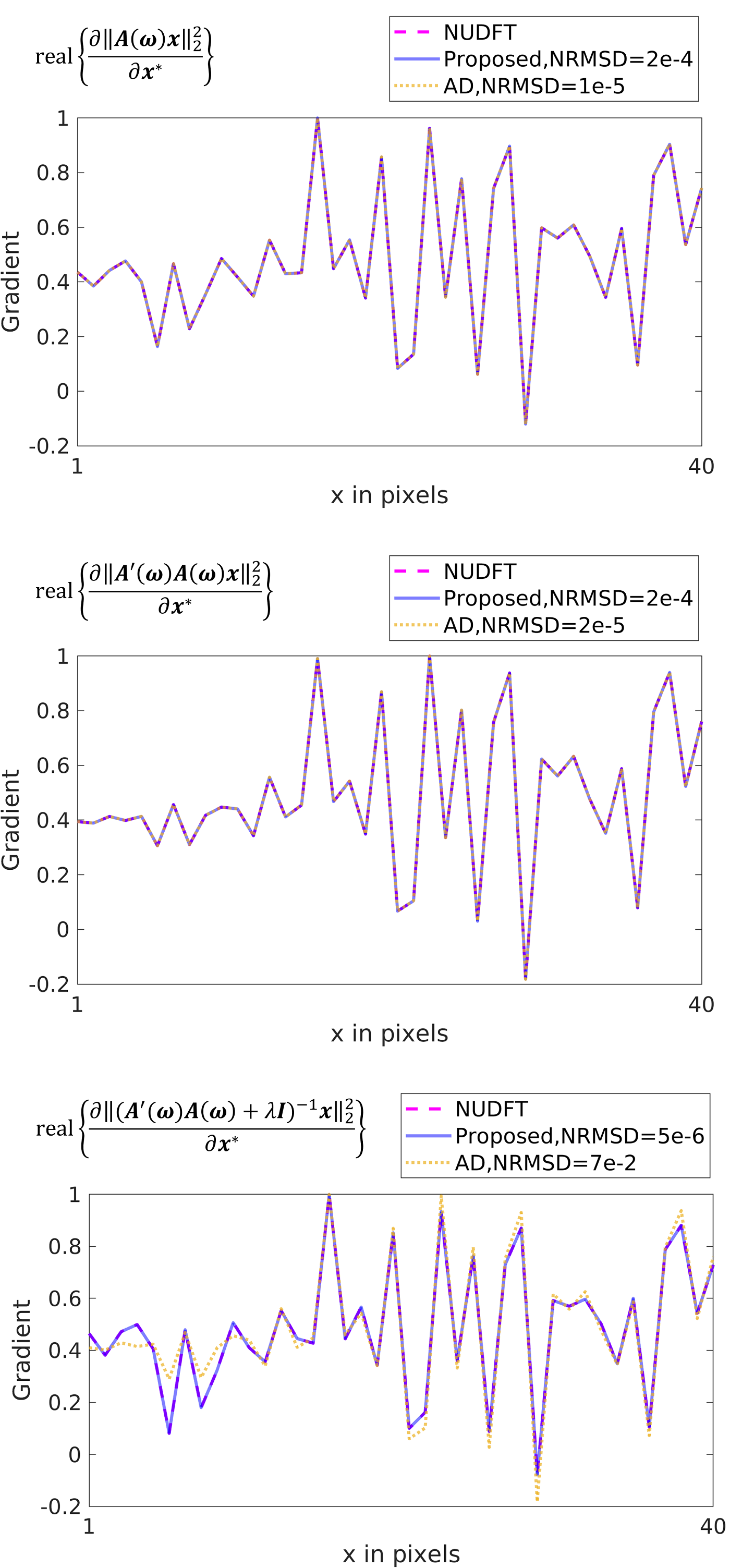
Figure 1: Examples of gradients w.r.t. $\bm{x}^{*}$ (the real part is plotted). Plots show one representative row of a $40\times 40$ matrix (rescaled to [-1,1]). The rows are the forward, Gram, and PSD inverse operator cases. The horizontal axis is the pixel index. The legend reports the normalized root-mean-square difference (NRMSD) compared with the reference NUDFT calculation.

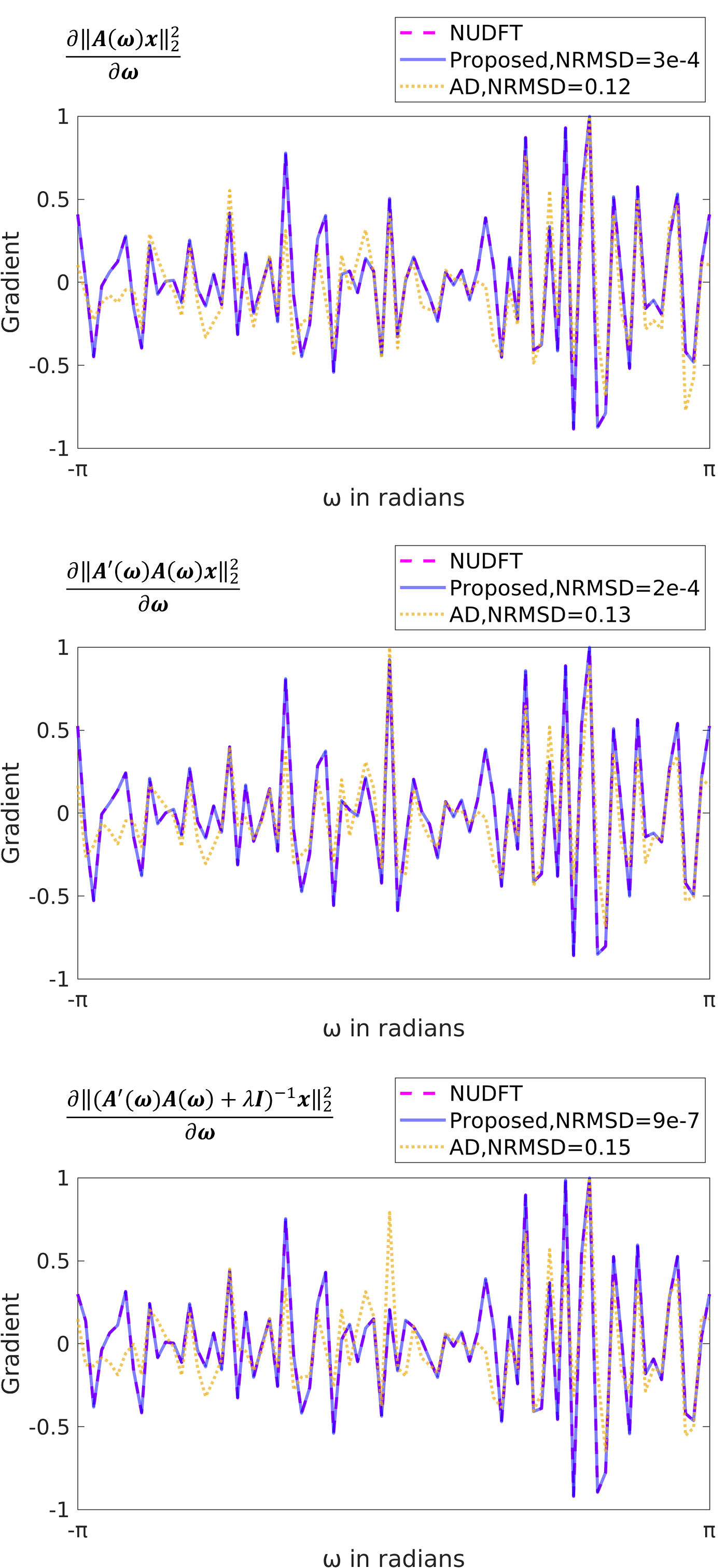
Figure 2: Examples of gradients w.r.t. $\bm{\omega}$. Plots show one spoke of 80 points (rescaled to [-1,1]). The rows are the forward, Gram, and PSD inverse operator cases. The proposed approximation better matches the gradient of the NUDFT. The legend reports the normalized root-mean-square difference (NRMSD) compared with the reference NUDFT calculation. The proposed approach has at least $400\times$ smaller NRMSD for this nonlinear case.

Fig. 1 and Fig. 2 illustrate representative profiles of the gradients w.r.t. $\bm{x}$ and $\bm{\omega}$. For $\bm{\omega}$, the auto-differentiation (method 1) approach has larger deviations from method 3 (NUDFT) because of the non-differentiability of interpolation operations w.r.t. coordinates. For the gradient w.r.t. $\bm{x}$, both method 1 and method 2 generate accurate results for forward and Gram operators. The reason is that in method 1 (auto-diff), the interpolation operation w.r.t $\bm{x}$ is linear, hence accurately differentiable. For the PSD inverse, method 1 led to a slightly inaccurate gradient, stemming from the accumulated errors of backpropagating CG iterations.

Table I and Table II compare the time and memory cost of methods 1 (auto-diff) and 2 (proposed). The CPU is Intel(R) Xeon(R) Gold 6138 CPU @ 2.00GHz and the GPU is an Nvidia(R) RTX2080Ti. We used PyTorch 1.9.1 and torchkbnufft 1.1.0. The memory usage was tracked by torch.cuda.max_memory_allocated on Nvidia GPUs. We implemented the numerical experiments with torchkbnufft [46] and MIRTorch toolboxes.

Our method is much faster than auto-differentiation on both GPUs and CPUs, and uses less memory. Importantly, the PSD inverse Jacobian is impractical for the 3D case, whereas the proposed approach fit comfortably in GPU’s onboard memory.

TABLE I: Computation time of the test case.

	Gram		Inverse
	auto-diff	proposed	auto-diff	proposed
Large image - GPU	0.3s	0.2s	4.3s	2.5s
Small image - GPU	0.1s	0.1s	1.3s	0.9s
Large image - CPU	5.2s	1.7s	276.2s	48.5s
Small image - CPU	0.8s	0.5s	27.4s	6.9s
Large size: $400\times 400$; small size: $40\times 40$
20 CG iterations were applied in the PSD inverse cases.

TABLE II: Memory use of the test case.

	Gram		Inverse
	standard	proposed	standard	proposed
Small	3.1MB	2.8MB	145.7MB	2.9MB
Large	375.9MB	267.5MB	5673.2MB	272.0MB
3D	N/A	10.1GB	N/A	10.8GB
Large size: $400\times 400$; small size: $40\times 40$;
3D size: $200\times 200\times 100$.
N/A: the memory usage was too large for a single GPU.
20 CG iterations were applied in the PSD inverse cases.

IV-B MRI Trajectory Optimization

This experiment optimized the MRI sampling trajectory using the proposed Jacobian approximations and stochastic optimization. The reconstruction methods (15) here consider two types of algorithms, namely smooth (regularized) least-squares reconstruction and sparsity-based reconstruction.

The smooth reconstruction method uses the cost function

$$\Psi(\bm{x})=\frac{1}{2}\|\bm{E}(\bm{\omega})\bm{x}-\bm{y}\|_{2}^{2}+\frac{\lambda}{2}\|\bm{T}\bm{x}\|_{2}^{2},$$

where $\bm{T}$ is a finite-difference operator encouraging smoothness. Correspondingly, the reconstructed image is:

$$\bm{x}_{K}=(\bm{E}^{\prime}\bm{E}+\lambda\bm{T}^{\prime}\bm{T})^{-1}\bm{E}^{\prime}\bm{y},$$

which we solved using CG. The following sections refer to this method as quadratic penalized least-squares (QPLS). We also implemented a simpler case, where $\bm{T}=\bm{I}$, which is referred as CG-SENSE [47]. In both scenarios, we set $\lambda$ to $10^{-3}$ empirically and still applied 20 CG iterations. The initialization of CG used the density compensated reconstruction [48].

The sparsity-based compressed (CS) sensing algorithm adopts a wavelets-based sparsity penalty, and has the following objective function

$$\Psi(\bm{x})=\frac{1}{2}\|\bm{E}(\bm{\omega})\bm{x}-\bm{y}\|_{2}^{2}+\lambda\|\bm{W}\bm{x}\|_{1},$$

where $\bm{W}$ is an orthogonal DWT matrix and we set $\lambda=10^{-5}$ empirically. We used 40 iterations of the proximal optimized gradient method (POGM) [49, 50] to solve this non-smooth optimization problem.

For the purpose of comparing trajectories and image quality, we also applied the proposed approximations to an unrolled neural network (UNN) reconstruction method that followed the definition of [39] ([24] extends it to non-Cartesian cases.) We used the same network configuration as in [24].

To optimize the k-space trajectory for each of these reconstruction methods, the training loss (16) is:

$$L(\bm{\omega})= \left\|\bm{x}_{K}(\bm{\omega})-\bm{x}^{\mathrm{true}}\right\|_{2}^{2}$$

$$+\mu_{1}\bm{\phi}_{\gamma\Delta tg_{\max}}(|\bm{D}_{1}\bm{\omega}|)+\mu_{2}\bm{\phi}_{\gamma\Delta t^{2}s_{\max}}(|\bm{D}_{2}\bm{\omega}|),$$

where $\bm{x}^{\mathrm{true}}$ is the conjugate phase reconstruction of fully sampled Cartesian data [51]. The second and third terms applied a soft constraint on gradient strength and slew rate according to [24, Eqn. 2], where $\bm{\phi}_{\lambda}(|\bm{x}|)=\sum\max(|\bm{x}|-\lambda,0)$. The maximum gradient strength ($g_{\max}$) was 5 Gauss/cm and the maximum slew rate ($s_{\max}$) was 15 Gauss/cm/ms. $\mu_{1}=\mu_{2}=10$. We estimated sensitivity maps in $\bm{E}$ using ESPIRiT [52], and simulated noiseless raw signals $\bm{y}=\bm{E}(\bm{\omega})\bm{x}^{\mathrm{true}}$ retrospectively w.r.t. candidate trajectories. The training used the fastMRI brain dataset [53] containing 15902 T1w slices, 16020 T2w slices, and 3311 FLAIR slices cropped to size $320\times 320$. The number of coils ranges from 2 to 28. We used the Adam optimizer [54], with step size $10^{-4}$ and mini-batch size $12$. We used 6 epochs for training model-based methods (CG-SENSE, QPLS and CS) and 60 epochs for the UNN training. The initialization of learned trajectories was an under-sampled radial trajectory in all experiments. The initialization had 16 “spokes” and each spoke was 5ms long with 1280 sampling points. We also adopted the k-space parameterization trick detailed in [24, Eqn. 3] to avoid sub-optimal local minima, and parameterized each shot with 40 quadratic spline kernels.

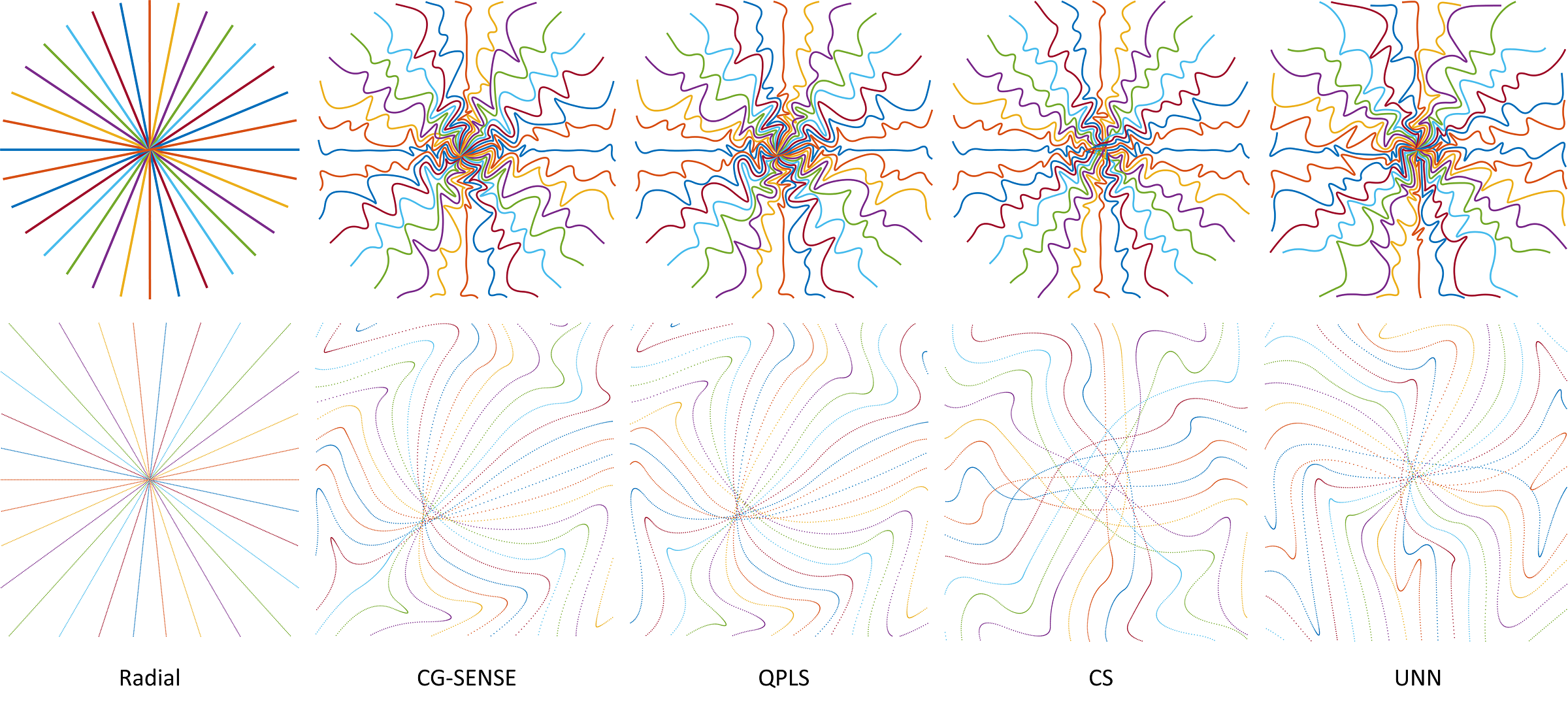
Figure 3: Optimized sampling trajectories for several iterative reconstruction methods. The left column shows the uniform radial initialization. The second row shows the $8\times$ zoomed-in central k-space.

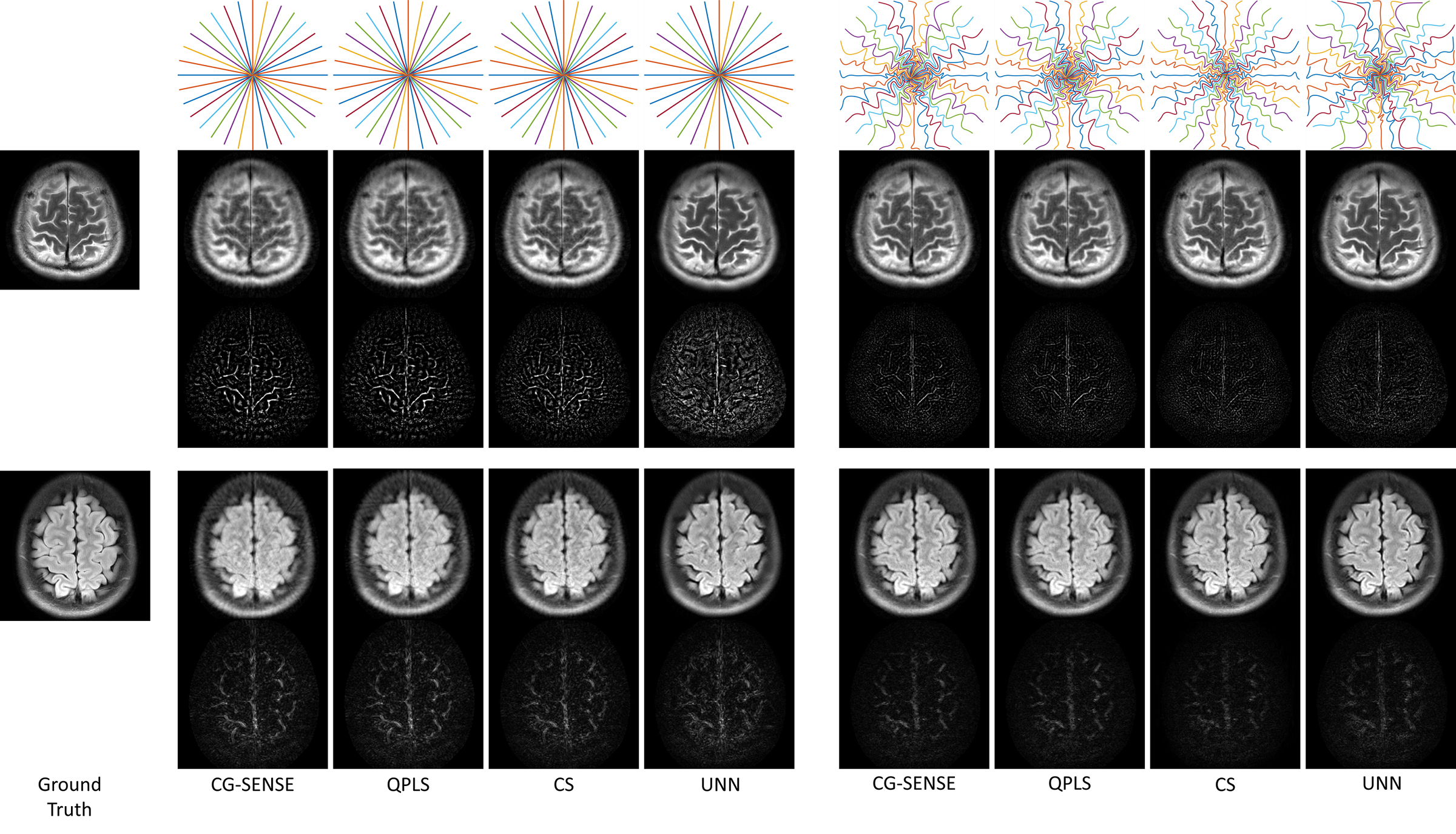
Figure 4: Examples of the reconstructed images with unoptimized (left) and optimized trajectories (right). Rows 3 and 5 show corresponding error maps.

Fig. 3 showcases the trajectories optimized for each of the reconstruction methods. The centers of trajectories optimized with quadratic regularizers (CG-SENSE and QPLS) are not aligned with the k-space origin. We hypothesize that regularizers (and corresponding iterative algorithms) handle image phases differently, resulting in distinct trajectory centers.

Table III reports the average image reconstruction quality (PSNR and SSIM [55], fully sampled image as the ground truth) on 500 test slices. It also showcases the image quality of these learned trajectories with reconstruction methods different from the training phase. All learned trajectories led to improved reconstruction quality compared to the initial radial trajectory (unopt.), even with different reconstruction methods. Importantly, the same reconstruction algorithm across training and test led to the greatest improvement (the bold diagonal entries). Fig. 4 shows reconstruction examples.

TABLE III: Average reconstruction quality on test set with trajectories learned for different reconstruction methods.

SSIM
	QPLS	SENSE	CS	UNN	unopt.
QPLS	0.963	0.963	0.962	0.961	0.947
SENSE	0.964	0.964	0.963	0.961	0.946
CS	0.962	0.963	0.966	0.964	0.946
UNN	0.960	0.960	0.958	0.964	0.950
PSNR (in dB)
	QPLS	SENSE	CS	UNN	unopt.
QPLS	35.1	35.1	34.9	35.0	33.1
SENSE	35.2	35.2	34.9	35.1	33.1
CS	34.8	34.9	35.4	35.2	33.0
UNN	34.6	34.6	34.5	35.0	33.5
Learn: the reconstruction method the trajectory is jointly trained with.
Test: the reconstruction method in the test phase.
unopt.: the undersampled radial trajectory (unoptimized initialization).

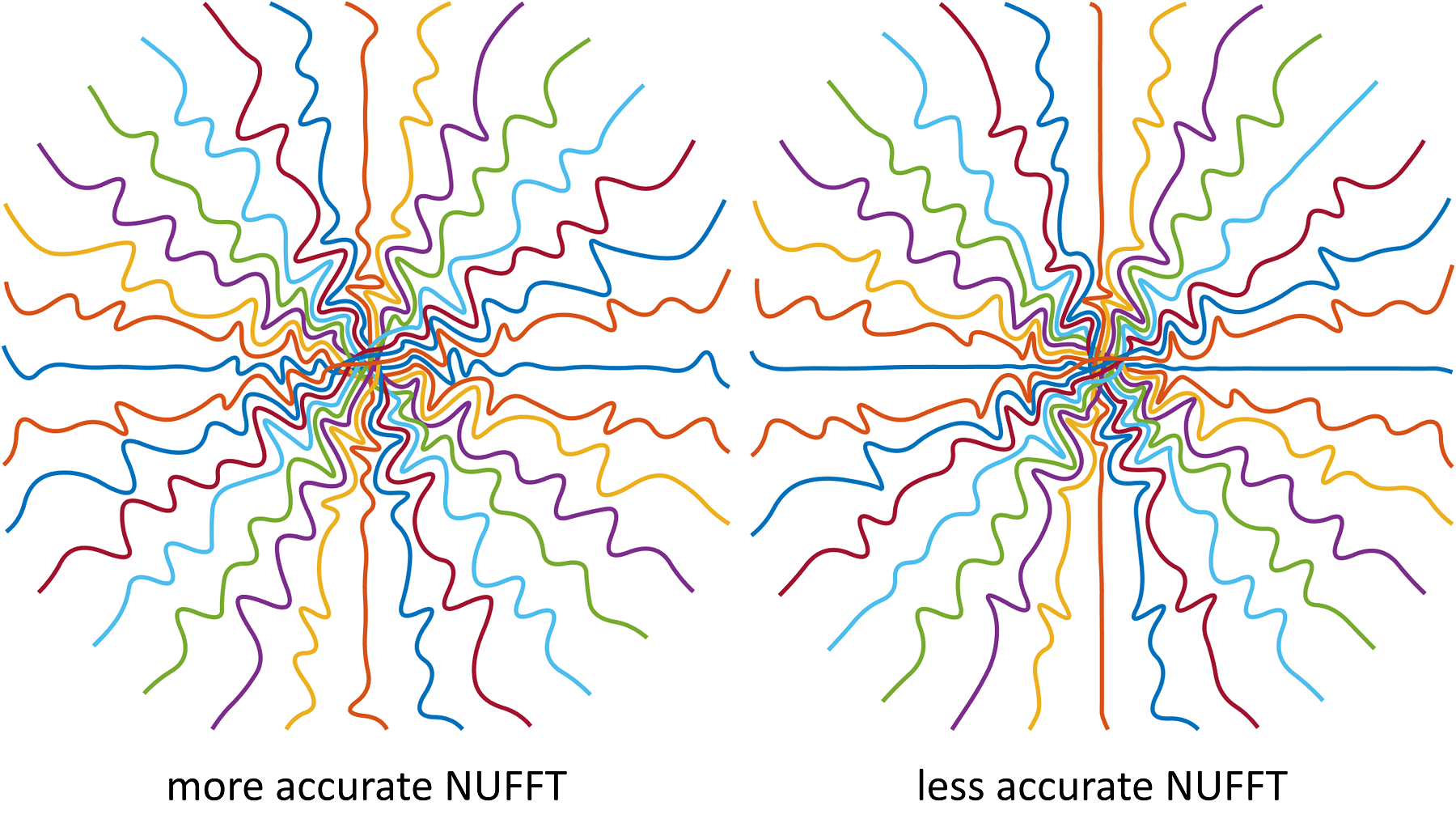
Figure 5: Learned trajectories with different NUFFT accuracies.

IV-C Accelerated Learning with Low-Accuracy NUFFT

The major computation cost of trajectory learning is proportional to NUFFTs and their Jacobian calculations. An empirical acceleration method is to use faster NUFFT approximations (low over-sampling factors and/or small interpolation neighborhoods) in training. Later, when the learned trajectory is deployed on test data or prospectively acquired data, one could use default NUFFT accuracy. We investigated learning trajectories with two different NUFFT accuracies: (1) gridding size = $1.25\times$ image size, interpolation kernel size = 5 and (2) gridding size = $2\times$ image size, interpolation kernel size = 6 which is a commonly used setting. On our GPUs, the lower-accuracy setting was $1.4\times$ faster than the higher-accuracy one. We used the CS-based reconstruction and corresponding training strategy described in the previous subsection. Fig. 5 shows the trajectory optimized for the two NUFFT accuracy levels. To compare the trajectory optimized by these two settings, we used the reconstruction image quality as the evaluation metric. We simulated and reconstructed images using the two trajectories on the test data (same as the previous experiment). The trajectories optimized with the “low accuracy” and “high accuracy” NUFFT had mean PSNR values of 35.4$\pm$4.6 dB and 35.4$\pm$4.7 dB.

V Discussion

This paper presents a model-based approximation of Jacobian matrices involving NUFFTs. Compared to direct auto-differentiation, the proposed method is faster, needs less memory, and better approximates the reference NUDFT results. As discussed in II-B, the error of auto-differentiation is not a software limitation, but rather a problem that stems from the non-differentiability of interpolation or lookup table operations. NUFFT alternatives such as re-gridding or filtered back-projection also suffer from similar non-differentiability issues and are less effective than (NUFFT-based) iterative reconstruction. Our previous studies [24, Fig. 14] compared the trajectory optimization results of the proposed method and standard auto-differentiation. The trajectory optimized by the proposed approximation generated superior image quality, and conformed better to the empirical criteria [56, 57]: sampling points should not overlap or be too distant from each other.

Sampling patterns learned with different reconstruction methods showed distinct characteristics in §IV-B. This phenomenon was also observed in previous literature [8, 10]. The differences in sampling patterns may stem from different regularizers, as well as different iterative algorithms. Importantly, as shown in Table III, synergistic sampling and reconstruction led to the best image quality. Several previous studies [22, 24, 23] only used NN-based reconstruction methods, while the stability and generalizability of NN-based reconstruction are still being investigated. In comparison, using our method delineated in §III, one may optimize trajectories for model-based reconstruction methods that may be more robust. Our results show that with a suitably tailored sampling pattern, traditional model-based reconstruction can compete with NN-based reconstruction, reinforcing related observations in recent studies [58]. Additionally, sampling optimization for model-based reconstruction requires less training data than for NN-based reconstruction. This property is beneficial for medical imaging where the data availability is often limited.

The training used discrete-space image datasets, whereas the actual objects in practice are continuous. Ideally, using an accurate continuous image model could better approximate the actual situation. This implicit bias is common for learning-based methods, and may lead to suboptimal results, such as the backtracking in the edge/corner of k-space (Fig. 3). The training also ignored physical processes such as relaxation and magnetization transfer. Future studies may consider these processes in the forward system model. The mismatch or domain shift from training to prospective scans may influence the results. For example, there exist differences in protocols (RF pulses, FOVs, and resolutions), hardware (field strengths and Tx/Rx coils), system imperfections (eddy currents, gradient non-linearity, and inhomogeneity), demography, and pathology. Our previous studies [24] tested the optimized trajectory in a prospective in-vivo experiment, and discussed practical issues, including eddy currents, and contrast/SNR mismatch between the training set and prospective protocols. Subsequent studies should evaluate the robustness of learned sampling trajectories in more scenarios.

This appendix analyzes the error of approximations based on (5) and (6), by comparing Jacobians computed when $\bm{A}$ is an exact NUDFT to those for an NUFFT, denoted $\bm{\tilde{A}}$. For simplicity, the analysis is 1D, though the conclusion extends easily to multi-dimensional NUFFTs.

The system matrix $\bm{A}\in\mathbb{C}^{M\times N}$ has elements

$$a_{mn}=\mathrm{e}^{-\imath\omega_{m}n},\quad m=1,\ldots,M,\quad n=1,\ldots,N.$$

Typically, an NUFFT involves three steps. The first step applies scaling factors $s_{n}$ to the signal $x_{n}$. The second step applies a $K$-point FFT to the scaled signal, where $K\geq N$ via zero-padding. The third step interpolates $K$ frequency locations into $M$ sampling locations of $\bm{\omega}$. For efficiency, the interpolator usually has finite support, denoted $J>0$. The NUFFT $\bm{\tilde{A}}$ has elements as follows:

$$\tilde{a}_{mn}=\sum_{j=1}^{J}u_{j}^{*}(\omega_{m})\,s_{n}\,\mathrm{e}^{-\imath\gamma\,(k_{m}+j)\,n},$$

where $u$ denotes interpolation coefficients, $k_{m}$ is an element-wise offset, and $\gamma=2\pi/K$ [6].

Define the NUFFT error matrix as $\bm{E}=\bm{\tilde{A}}-\bm{A}$. The worst-case NUFFT error has a bound that can be written as

$$\left\|\bm{E}\bm{x}\right\|_{\infty}\leq\varepsilon_{p}\left\|\bm{x}\right\|_{2},$$

where $\varepsilon_{p}$ is tabulated numerically for various choices of interpolation parameters $p$, e.g., in [6, Fig. 12].

The Jacobian of the forward operator (5) is

$$\bm{J}=\frac{\partial\bm{A}\bm{x}}{\partial\bm{\omega}}=-\imath\,\mathrm{diag}\!\left\{\bm{A}(\bm{x}\odot\bm{r})\right\}.$$

Let $\bm{\tilde{J}}$ denote the case where an NUFFT is applied. Since the backpropagation uses Jacobians in the JVP calculation, here we analyze the error of JVPs using $\bm{J}$ and $\bm{\tilde{J}}$. We define the worst-case relative error for a JVP with a (gradient) vector $\bm{v}$ as follows:

$$E_{1}(\bm{\omega},\bm{x},p) \triangleq\max_{\left\|\bm{v}\right\|_{\infty}=1}\|\bm{\tilde{J}}\bm{v}-\bm{J}\bm{v}\|_{\infty}/\left\|\bm{x}\right\|_{2}$$

$$=\max_{\left\|\bm{v}\right\|_{\infty}=1}\left\|(\bm{E}\,(\bm{x}\odot\bm{r}))\odot\bm{v}\right\|_{\infty}/\left\|\bm{x}\right\|_{2}$$

$$=\left\|\bm{E}\,(\bm{x}\odot\bm{r})\right\|_{\infty}/\left\|\bm{x}\right\|_{2}$$

$$\leq\varepsilon_{p}\left\|\bm{x}\odot\bm{r}\right\|_{2}/\left\|\bm{x}\right\|_{2}\leq\varepsilon_{p}\left\|\bm{r}\right\|_{\infty}.$$

Similarly, the worst-case relative error of a JVP with (6) is bounded by

$$E_{2}(\bm{\omega},\bm{x},p) \triangleq\max_{\left\|\bm{v}\right\|_{\infty}=1}\left\|\mathrm{diag}\!\left\{\bm{r}\right\}\bm{E}^{\prime}\mathrm{diag}\!\left\{\bm{y}\right\}\bm{v}\right\|_{\infty}/\left\|\bm{y}\right\|_{2}$$

$$\leq\max_{\left\|\bm{v}\right\|_{\infty}=1}\left\|\bm{r}\right\|_{\infty}\left\|\bm{E}^{\prime}(\bm{y}\odot\bm{v})\right\|_{\infty}/\left\|\bm{y}\right\|_{2}$$

$$\leq\varepsilon_{p}\left\|\bm{r}\right\|_{\infty}\max_{\left\|\bm{v}\right\|_{\infty}=1}\left\|\bm{y}\odot\bm{v}\right\|_{2}/\left\|\bm{y}\right\|_{2}$$

$$\leq\varepsilon_{p}\left\|\bm{r}\right\|_{\infty}\left\|\bm{y}\right\|_{2}/\left\|\bm{y}\right\|_{2}\leq\varepsilon_{p}\left\|\bm{r}\right\|_{\infty}.$$

In both cases, the worst-case error of the NUFFT approximation for a JVP is bounded by the usual NUFFT error multiplied by a constant $\left\|\bm{r}\right\|_{\infty}$ that is usually half of the field of view (FOV) in imaging applications. This constant is expected from unit analysis. If the sampling grid $r_{j}$ has a unit in cm, then the sample locations $\bm{\omega}$ have units in radians/cm. Corresponding, the Jacobian matrices in (5) and (6) have units in cm, because $\bm{A}$ is unitless. The NUFFT error $\varepsilon_{p}$ is unitless, so there is an $\bm{r}$-related factor in the JVP error $E$. In other words, the error bounds above depend on the choice of units. One could express the FOV in voxels to get the unitless error bound $\varepsilon_{p}N/2$. However, the accuracy of JVPs does not necessarily deteriorate with larger $N$. Above we normalized the error by $\left\|\bm{x}\right\|_{2}$ or $\left\|\bm{y}\right\|_{2}$, whereas the Jacobians are “scaled” with $\left\|\bm{x}\odot\bm{r}\right\|_{2}$ or $\left\|\bm{y}\right\|_{2}\left\|\bm{r}\right\|_{2}$. A relative error could better describe the effect on optimization.

An alternate definition uses the worst-case in the numerator relative to an average case in the denominator, considering the stochastic gradient descent-like optimizers. For example, this relative error for the JVP of Jacobian (5) is

$$\epsilon \triangleq\frac{\max_{\left\|\bm{x}\right\|_{2}=1}\|\bm{\tilde{J}}-\bm{J}\|_{\mathrm{F}}}{\sqrt{\mathsf{E}_{p(\bm{x})}\![\left\|\bm{J}\right\|_{\mathrm{F}}^{2}]}}=\frac{\max_{\left\|\bm{x}\right\|_{2}=1}\left\|\bm{E}\,(\bm{x}\odot\bm{r})\right\|_{2}}{\sqrt{\mathsf{E}_{p(\bm{x})}\![\left\|\bm{A}\,(\bm{x}\odot\bm{r})\right\|_{2}^{2}]}}$$

$$\leq\frac{\max_{\left\|\bm{x}\right\|_{2}=1}\sqrt{M}\left\|\bm{E}\,(\bm{x}\odot\bm{r})\right\|_{\infty}}{\sqrt{\mathsf{E}_{p(\bm{x})}\![\left\|\bm{A}\,(\bm{x}\odot\bm{r})\right\|_{2}^{2}]}}\leq\frac{\sqrt{M}\varepsilon_{p}\left\|\bm{r}\right\|_{\infty}}{\sqrt{\mathsf{E}_{p(\bm{x})}\![\left\|\bm{A}\,(\bm{x}\odot\bm{r})\right\|_{2}^{2}]}},$$

where $\mathsf{E}_{p(\bm{x})}\![\cdot]$ denotes expectation w.r.t. a certain distribution $p(\bm{x})$. For parity with the unit sphere constraint in the numerator, we consider the case where $p(\cdot)$ is the random distribution on the unit $N$-sphere. Use the cyclic property of the trace:

$$\left\|\bm{A}\,(\bm{x}\odot\bm{r})\right\|_{2}^{2} =\bm{x}^{\prime}\mathrm{diag}\!\left\{\bm{r}\right\}\bm{A}^{\prime}\bm{A}\mathrm{diag}\!\left\{\bm{r}\right\}\bm{x}$$

$$=\mathrm{Tr}\!\left\{\mathrm{diag}\!\left\{\bm{r}\right\}\bm{A}^{\prime}\bm{A}\mathrm{diag}\!\left\{\bm{r}\right\}\bm{x}\bm{x}^{\prime}\right\}.$$

Since the covariance of random points on the $N$-sphere is $(1/N)\bm{I}$, the denominator’s expectation is

$$\mathsf{E}_{p(\bm{x})}\![\left\|\bm{A}\,(\bm{x}\odot\bm{r})\right\|_{2}^{2}] =\mathrm{Tr}\!\left\{\mathrm{diag}\!\left\{\bm{r}\right\}\bm{A}^{\prime}\bm{A}\mathrm{diag}\!\left\{\bm{r}\right\}\mathsf{E}_{p(\bm{x})}\![\bm{x}\bm{x}^{\prime}]\right\}$$

$$=\frac{1}{N}\mathrm{Tr}\!\left\{\mathrm{diag}\!\left\{\bm{r}\right\}\bm{A}^{\prime}\bm{A}\mathrm{diag}\!\left\{\bm{r}\right\}\right\}$$

$$=\frac{1}{N}\sum_{j}r_{j}^{2}[\bm{A}^{\prime}\bm{A}]_{jj}=\frac{M}{N}\sum_{j}r_{j}^{2}=\frac{M}{N}\left\|\bm{r}\right\|_{2}^{2}.$$

Thus we have the following bound for the relative error:

$$\epsilon\leq\frac{\sqrt{M}\varepsilon_{p}\left\|\bm{r}\right\|_{\infty}}{\sqrt{M/N}\left\|\bm{r}\right\|_{2}}=\varepsilon_{p}\sqrt{N}\frac{\left\|\bm{r}\right\|_{\infty}}{\left\|\bm{r}\right\|_{2}}\leq\varepsilon_{p}\sqrt{N}.$$

Note that the bound can be tighter when considering specific formulations of $\bm{r}$. Similarly, for the Jacobian operator (6), the alternate error of the JVP is

$$\epsilon\leq\varepsilon_{p}\sqrt{M}.$$

References

- [1] D. C. Munson and J. L. Sanz, “Image reconstruction from frequency-offset Fourier data,” Proc. IEEE, vol. 72, no. 6, pp. 661–9, Jun. 1984.
- [2] M. M. Bronstein, A. M. Bronstein, M. Zibulevsky, and H. Azhari, “Reconstruction in diffraction ultrasound tomography using nonuniform FFT,” IEEE Trans. Med. Imag., vol. 21, no. 11, pp. 1395–1401, Nov. 2002.
- [3] S. Matej, J. A. Fessler, and I. G. Kazantsev, “Iterative tomographic image reconstruction using Fourier-based forward and back- projectors,” IEEE Trans. Med. Imag., vol. 23, no. 4, pp. 401–12, Apr. 2004.
- [4] K. L. Wright, J. I. Hamilton, M. A. Griswold, V. Gulani, and N. Seiberlich, “Non-Cartesian parallel imaging reconstruction,” J. Magn. Reson. Imag., vol. 40, no. 5, pp. 1022–1040, 2014.
- [5] J. A. Fessler, “Model-based image reconstruction for MRI,” IEEE Sig. Proc. Mag., vol. 27, no. 4, pp. 81–9, Jul. 2010.
- [6] J. A. Fessler and B. P. Sutton, “Nonuniform fast Fourier transforms using min-fmax interpolation,” IEEE Trans. Sig. Proc., vol. 51, no. 2, pp. 560–74, Feb. 2003.
- [7] Z. Yang and M. Jacob, “Mean square optimal NUFFT approximation for efficient non-Cartesian MRI reconstruction,” J. Mag. Res., vol. 242, pp. 126–35, May 2014.
- [8] M. V. W. Zibetti, G. T. Herman, and R. R. Regatte, “Fast data-driven learning of parallel MRI sampling patterns for large scale problems,” Sci Rep, vol. 11, no. 1, p. 19312, Sep. 2021.
- [9] T. Sanchez et al., “Scalable learning-based sampling optimization for compressive dynamic MRI,” in 2020 IEEE Intl. Conf. on Acous., Speech and Sig. Proc. (ICASSP), May 2020, pp. 8584–8588.
- [10] B. Gözcü, T. Sanchez, and V. Cevher, “Rethinking Sampling in Parallel MRI: A Data-Driven Approach,” in 2019 27th Euro. Sig. Proc. Conf. (EUSIPCO), Sep. 2019, pp. 1–5.
- [11] Y. Cao and D. N. Levin, “Feature-recognizing MRI,” Magn. Reson. Med., vol. 30, no. 3, pp. 305–317, 1993.
- [12] F. Knoll, C. Clason, C. Diwoky, and R. Stollberger, “Adapted random sampling patterns for accelerated MRI,” Mag. Res. Mat. Phys. Bio. Med., vol. 24, no. 1, pp. 43–50, Feb. 2011.
- [13] C. D. Bahadir, A. Q. Wang, A. V. Dalca, and M. R. Sabuncu, “Deep-learning-based optimization of the under-sampling pattern in MRI,” IEEE Trans. Comput. Imag., vol. 6, pp. 1139–1152, 2020.
- [14] F. Sherry, M. Benning, J. C. D. . Reyes, M. J. Graves, G. Maierhofer, G. Williams, C.-B. Schonlieb, and M. J. Ehrhardt, “Learning the sampling pattern for MRI,” IEEE Trans. Med. Imag., vol. 39, no. 12, pp. 4310–21, Dec. 2020.
- [15] I. A. M. Huijben, B. S. Veeling, and R. J. G. van Sloun, “Learning sampling and model-based signal recovery for compressed sensing MRI,” in 2020 IEEE Intl. Conf. on Acous., Speech and Sig. Proc. (ICASSP), May 2020, pp. 8906–8910.
- [16] M. Seeger, H. Nickisch, R. Pohmann, and B. Schölkopf, “Optimization of k-space trajectories for compressed sensing by Bayesian experimental design,” Magn. Reson. Med., vol. 63, no. 1, pp. 116–126, 2010.
- [17] J. P. Haldar and D. Kim, “OEDIPUS: An Experiment Design Framework for Sparsity-Constrained MRI,” IEEE Trans. Med. Imaging, vol. 38, no. 7, pp. 1545–1558, Jul. 2019.
- [18] M. von Kienlin and R. Mejia, “Spectral localization with optimal pointspread function,” J. Magn. Reson. (1969), vol. 94, no. 2, pp. 268–287, Sep. 1991.
- [19] Y. Gao and S. Reeves, “Optimal k-space sampling in MRSI for images with a limited region of support,” IEEE Trans. Med. Imag., vol. 19, no. 12, pp. 1168–1178, Dec. 2000.
- [20] D. Xu, M. Jacob, and Z. Liang, “Optimal sampling of k-space with cartesian grids for parallel MR imaging,” in Proc. Intl. Soc. Mag. Res. Med., 2005, p. 2450.
- [21] E. Levine and B. Hargreaves, “On-the-fly adaptive k-Space sampling for linear MRI reconstruction using moment-based spectral analysis,” IEEE Trans. Med. Imag., vol. 37, no. 2, pp. 557–567, 2017.
- [22] T. Weiss, O. Senouf, S. Vedula, O. Michailovich, M. Zibulevsky, and A. Bronstein, “PILOT: Physics-informed learned optimized trajectories for accelerated MRI,” MELBA, pp. 1–23, 2021.
- [23] H. K. Aggarwal and M. Jacob, “J-MoDL: Joint model-based deep learning for optimized sampling and reconstruction,” IEEE J. Sel. Top. Sig. Proc., vol. 14, no. 6, pp. 1151–62, Oct. 2020.
- [24] G. Wang, T. Luo, J.-F. Nielsen, D. C. Noll, and J. A. Fessler, “B-Spline Parameterized Joint Optimization of Reconstruction and K-Space Trajectories (BJORK) for Accelerated 2D MRI,” IEEE Trans. Med. Imag., vol. 41, no. 9, pp. 2318–2330, Sep. 2022.
- [25] E. Scope Crafts, H. Lu, H. Ye, L. L. Wald, and B. Zhao, “An efficient approach to optimal experimental design for magnetic resonance fingerprinting with B-splines,” Magn. Reson. Med., vol. 88, no. 1, pp. 239–253, 2022.
- [26] S. P. Jordan, S. Hu, I. Rozada, D. F. McGivney, R. Boyacioglu, D. C. Jacob, S. Huang, M. Beverland, H. G. Katzgraber, M. Troyer et al., “Automated design of pulse sequences for magnetic resonance fingerprinting using physics-inspired optimization,” Proc. Natl. Acad. Sci, vol. 118, no. 40, p. e2020516118, 2021.
- [27] B. Dale, M. Wendt, and J. L. Duerk, “A rapid look-up table method for reconstructing MR images from arbitrary K-space trajectories,” IEEE Trans. Med. Imag., vol. 20, no. 3, pp. 207–17, Mar. 2001.
- [28] P. J. Beatty, D. G. Nishimura, and J. M. Pauly, “Rapid gridding reconstruction with a minimal oversampling ratio,” IEEE Trans. Med. Imag., vol. 24, no. 6, pp. 799–808, Jun. 2005.
- [29] K. P. Pruessmann, M. Weiger, M. B. Scheidegger, and P. Boesiger, “SENSE: sensitivity encoding for fast MRI,” Magn. Reson. Med., vol. 42, no. 5, pp. 952–962, 1999.
- [30] B. Sutton, D. Noll, and J. Fessler, “Fast, iterative image reconstruction for MRI in the presence of field inhomogeneities,” IEEE Trans. Med. Imaging, vol. 22, no. 2, pp. 178–188, Feb. 2003.
- [31] M. Zehni, L. Donati, E. Soubies, Z. Zhao, and M. Unser, “Joint angular refinement and reconstruction for single-particle cryo-EM,” IEEE Trans. Im. Proc., vol. 29, pp. 6151–63, 2020.
- [32] G. Wang, D. C. Noll, and J. A. Fessler, “Reconstruction may benefit from tailored sampling trajectories: optimizing non-Cartesian trajectories for model-based reconstruction,” in Proc. Intl. Soc. Mag. Res. Med., 2022, p. 5011. [Online]. Available: https://submissions.mirasmart.com/ISMRM2022/Itinerary/Files/PDFFiles/5011.html
- [33] R. Remmert, Theory of complex functions. Springer Science & Business Media, 1991, vol. 122.
- [34] K. Kreutz-Delgado, “The complex gradient operator and the CR-calculus,” arXiv preprint arXiv:0906.4835, 2009.
- [35] A. Hjorungnes and D. Gesbert, “Complex-valued matrix differentiation: Techniques and key results,” IEEE Trans. Sig. Proc., vol. 55, no. 6, pp. 2740–2746, 2007.
- [36] Wikipedia contributors, “Numerator layout notation,” 2022, [Accessed 2022-11-08]. [Online]. Available: https://en.wikipedia.org/wiki/Matrix_calculus#Numerator-layout_notation
- [37] J. R. Magnus and H. Neudecker, Matrix differential calculus with applications in statistics and econometrics. John Wiley & Sons, 2019.
- [38] M. R. Hestenes, “Multiplier and gradient methods,” J. Optim. Theory Appl., vol. 4, no. 5, pp. 303–320, Nov. 1969.
- [39] H. K. Aggarwal, M. P. Mani, and M. Jacob, “MoDL: model-based deep learning architecture for inverse problems,” IEEE Trans. Med. Imag., vol. 38, no. 2, pp. 394–405, Feb. 2019.
- [40] S. Ramani and J. A. Fessler, “Parallel MR image reconstruction using augmented Lagrangian methods,” IEEE Trans. Med. Imag., vol. 30, no. 3, pp. 694–706, Mar. 2011.
- [41] S. H. Chan, X. Wang, and O. A. Elgendy, “Plug-and-play ADMM for image restoration: fixed-point convergence and applications,” IEEE Trans. Computational Imaging, vol. 3, no. 1, pp. 84–98, Mar. 2017.
- [42] J. A. Fessler, S. Lee, V. T. Olafsson, H. R. Shi, and D. C. Noll, “Toeplitz-based iterative image reconstruction for MRI with correction for magnetic field inhomogeneity,” IEEE Trans. Sig. Proc., vol. 53, no. 9, pp. 3393–402, Sep. 2005.
- [43] G. Wang, J.-F. Nielsen, J. A. Fessler, and D. C. Noll, “Stochastic optimization of 3D non-Cartesian sampling trajectory (SNOPY),” 2022. [Online]. Available: http://arxiv.org/abs/2209.11030
- [44] M. Lustig, D. L. Donoho, J. M. Santos, and J. M. Pauly, “Compressed sensing MRI,” IEEE Signal Process. Mag., vol. 25, no. 2, pp. 72–82, Mar. 2008.
- [45] J. R. Shewchuk et al., “An introduction to the conjugate gradient method without the agonizing pain,” 1994. [Online]. Available: https://www.cs.cmu.edu/~quake-papers/painless-conjugate-gradient.pdf
- [46] M. J. Muckley, R. Stern, T. Murrell, and F. Knoll, “TorchKbNufft: A high-level, hardware-agnostic non-uniform fast fourier transform,” in ISMRM Workshop on Data Sampling & Image Reconstruction, 2020.
- [47] O. Maier et al., “CG-SENSE revisited: Results from the first ISMRM reproducibility challenge,” Magn. Reson. Med., vol. 85, no. 4, pp. 1821–1839, 2021.
- [48] R. D. Hoge, R. K. Kwan, and G. Bruce Pike, “Density compensation functions for spiral MRI,” Magn. Reson. Med., vol. 38, no. 1, pp. 117–128, 1997.
- [49] D. Kim and J. A. Fessler, “Adaptive restart of the optimized gradient method for convex optimization,” J Optim Theory Appl, vol. 178, no. 1, pp. 240–263, Jul. 2018.
- [50] J. A. Fessler, “Optimization methods for MR image reconstruction,” IEEE Sig. Proc. Mag., vol. 37, no. 1, pp. 33–40, Jan. 2020.
- [51] D. C. Noll, J. A. Fessler, and B. P. Sutton, “Conjugate phase MRI reconstruction with spatially variant sample density correction,” IEEE Trans. Med. Imag., vol. 24, no. 3, pp. 325–336, 2005.
- [52] M. Uecker et al., “ESPIRiT - an eigenvalue approach to autocalibrating parallel MRI: where SENSE meets GRAPPA,” Mag. Reson. Med., vol. 71, no. 3, pp. 990–1001, Mar. 2014.
- [53] J. Zbontar et al., “fastMRI: An open dataset and benchmarks for accelerated MRI,” 2018. [Online]. Available: http://arxiv.org/abs/1811.08839
- [54] D. P. Kingma and J. Ba, “Adam: a method for stochastic optimization,” 2017. [Online]. Available: http://arxiv.org/abs/1412.6980
- [55] A. Horé and D. Ziou, “Image quality metrics: PSNR vs. SSIM,” in Intl. Conf. on Patn. Recog. (ICPR), Aug. 2010, pp. 2366–2369.
- [56] C. Lazarus et al., “SPARKLING: variable-density k-space filling curves for accelerated T2*-weighted MRI,” Mag. Res. Med., vol. 81, no. 6, pp. 3643–61, Jun. 2019.
- [57] C. Boyer, N. Chauffert, P. Ciuciu, J. Kahn, and P. Weiss, “On the generation of sampling schemes for magnetic resonance imaging,” SIAM J. Imaging Sci., vol. 9, no. 4, pp. 2039–2072, 2016.
- [58] H. Gu, B. Yaman, S. Moeller, J. Ellermann, K. Ugurbil, and M. Akcakaya, “Revisiting l1-wavelet compressed-sensing MRI in the era of deep learning,” Proc. Natl. Acad. Sci., vol. 119, no. 33, p. e2201062119, Aug. 2022.