Certainty Volume Prediction for Unsupervised Domain Adaptation

Abstract

Unsupervised domain adaptation (UDA) deals with the problem of classifying unlabeled target domain data while labeled data is only available for a different source domain. Unfortunately, commonly used classification methods cannot fulfill this task adequately due to the domain gap between the source and target data. In this paper, we propose a novel uncertainty-aware domain adaptation setup that models uncertainty as a multivariate Gaussian distribution in feature space. We show that our proposed uncertainty measure correlates with other common uncertainty quantifications and relates to smoothing the classifier’s decision boundary, therefore improving the generalization capabilities. We evaluate our proposed pipeline on challenging UDA datasets and achieve state-of-the-art results. Code for our method is available at https://gitlab.com/tringwald/cvp.

1 Introduction

In recent years, deep neural classification networks have been successfully applied to a wide variety of tasks. One key contribution to that success is the utilization of enormous amounts of labeled training data during the optimization process of such networks. While abundant labeled data might be readily available for a given source domain, more specialized data is often hard to obtain or too expensive to manually label for a desired target domain (e.gmedical data). Thus, past research [Zou et al.(2020)Zou, Shi, Li, Zhang, and Shi, Richter et al.(2016)Richter, Vineet, et al., Ringwald and Stiefelhagen(2021), Peng et al.(2017)Peng, Usman, Kaushik, Hoffman, Wang, and Saenko] proposed to generate synthetic data for the training of classifiers, as this would render the manual labeling process unnecessary. Unfortunately, current classification architectures cannot handle the domain shift between the source and target domain, leading to a significantly degraded classification accuracy.

Unsupervised domain adaptation (UDA) seeks to address this domain shift problem by adapting a model to the desired target domain while only given labeled data of the source domain. Recent work has tackled this problem from multiple different angles: Holistic image-level and pixel-level methods often try to manipulate the global appearance of a given source or target domain image, for example by applying style transfer or other image-to-image mapping algorithms [Hoffman et al.(2018)Hoffman, Tzeng, Park, Zhu, Isola, Saenko, Efros, and Darrell, Atapour-Abarghouei and Breckon(2018)]. At the feature-level, prior methods commonly focus on minimizing domain divergence measures [Kang et al.(2019)Kang, Jiang, Yang, and Hauptmann, Meng et al.(2018)Meng, Li, Gong, and Juang] or enforce source and target features to be indistinguishable through the means of adversarial training [Ganin and Lempitsky(2015), Pinheiro(2018)].

However, these methods often neglect the intrinsic uncertainty accompanying the unsupervised domain adaptation process: as no target domain labels are available, pseudo-labels have to be constructed, which is an inherently noisy task involving uncertainty. In this paper, we thus propose a novel feature-level unsupervised domain adaptation algorithm called Certainty Volume Prediction (CVP). CVP integrates uncertainty into the domain adaptation pipeline by modelling a multivariate Gaussian distribution around a given feature. The covariance matrix of said distribution is constructed in a way that reflects the model’s current certainty (or uncertainty) for a feature given the current training step. We achieve this by enforcing samples from the distribution to belong to the same class as the original feature. Therefore, features for which the model is more certain can be allotted higher variance values than uncertain features, due to their distance from the decision boundary.

Finally, we show that our proposed feature space method correlates with other common uncertainty measures in classifier space – such as Monte-Carlo Dropout [Gal and Ghahramani(2016)] – and relates to smoothing the decision boundary [Bartlett and Shawe-taylor(1998), Lee et al.(1995)Lee, Bartlett, and Williamson, Rodríguez et al.(2020)Rodríguez, Laradji, Drouin, and Lacoste] which has been linked to better generalization and robustness properties [Hindi and Al-Akhras(2011)]. In summary, our contributions are threefold: (i) We introduce our novel Certainty Volume Prediction algorithm for measuring uncertainty in feature space and show how it can help to improve a model’s domain adaptation capabilities. (ii) We show its correlation to other uncertainty measures such as Monte-Carlo Dropout. (iii) We show CVP’s state-of-the-art performance on multiple challenging datasets and link its increased generalization performance to the smoothness of the decision boundary.

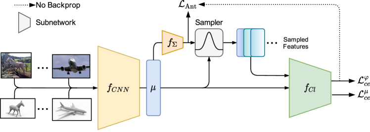
Figure 1: Overview of our proposed Certainty Volume Prediction (CVP) architecture. The predicted feature mean and covariance matrix predicted by the $f_{\Sigma}$ subnetwork are forwarded to the feature sampler, that draws additional samples according to the distribution. These samples and the original mean features are classified by the $f_{\text{Cl}}$ subnetwork and used for our proposed loss functions.

2 Related Work

Recent works in the area of domain adaptation have viewed the domain shift problem from multiple different angles: At a holistic image-level (often referred to as pixel-level), methods often try to find a common input or latent space in order to reuse the same classifier for both source and target domain. This can be achieved by the means of style transfer [Atapour-Abarghouei and Breckon(2018)] and related image-to-image translation methods [Hoffman et al.(2018)Hoffman, Tzeng, Park, Zhu, Isola, Saenko, Efros, and Darrell, Murez et al.(2018)Murez, Kolouri, Kriegman, Ramamoorthi, and Kim]. A domain-agnostic space can also be created at the feature-level instead of the image-level. For this, Ganin et alpropose their gradient reversal layer (RevGrad) in conjunction with a domain classifier, which enforces features from the source and target domain to be indistinguishable. Additionally, distribution divergence measures have been applied at the feature-level for the alignment of the source and target domain distributions: Long et al [Long et al.(2013)Long, Wang, Ding, Sun, and Yu] employ a maximum mean discrepancy (MMD) [Gretton et al.(2006)Gretton, Borgwardt, Rasch, Schölkopf, and Smola] based method in order to jointly adapt the marginal and conditional distributions. This idea of MMD-based optimization has recently been picked up again by Kang et al [Kang et al.(2019)Kang, Jiang, Yang, and Hauptmann] for their proposed CDD loss and is also used for regularization in the PUnDA framework by Gholami et al [Gholami et al.(2017)Gholami, Pavlovic, et al.]. Motivated by the results of Szegedy and Goodfellow [Szegedy et al.(2013)Szegedy, Zaremba, Sutskever, Bruna, Erhan, Goodfellow, and Fergus, Goodfellow et al.(2014)Goodfellow, Pouget-Abadie, Mirza, Xu, Warde-Farley, Ozair, Courville, and Bengio], adversarial approaches have also been investigated. In this subarea, Park et al [Park et al.(2018)Park, Park, Shin, and Moon] have applied adversarial dropout to improve generalization while Pinheiro [Pinheiro(2018)] proposes a categorical prototype-based domain-adversarial learning setup. Another orthogonal research directions was pursued by Chang et al [Chang et al.(2019)Chang, You, Seo, Kwak, and Han], who aim at capturing the different source and target distributions in domain-specific batch-normalization layers.

In this work, we focus on the integration of uncertainty into the domain adaptation pipeline. Related to this topic, Han et al [Han et al.(2019)Han, Zou, Gao, Wang, and Metaxas] proposed to calibrate the predictive uncertainty on the target domain data through the source domain uncertainties. They model this uncertainty in the classifier space and quantify it as the predicted Rényi entropy on the target domain data. Guan et al [Guan et al.(2021)Guan, Huang, Xiao, Lu, and Cao] propose the UaDAN framework that employs conditional adversarial learning for alignment of samples. They measure uncertainty as a proxy metric based on the alignment quality of samples and use this in the alignment process as well as their proposed curriculum learning setup. Furthermore, Ringwald et al [Ringwald and Stiefelhagen(2020)] propose the UFAL architecture, which measures uncertainty through Monte-Carlo Dropout (MCD) in classifier space. They then utilize this uncertainty for alignment of features in an Euclidean feature space and also for a curriculum learning-like filtering step.

Unlike the aforementioned approaches, our Certainty Volume Prediction (CVP) framework does not use post hoc measures for uncertainty but instead directly models uncertainty as a multivariate normal distribution in feature space, which is integrated in the backpropagation path of our model and can therefore be optimized during training. We show that our proposed uncertainty measure in feature space correlates with commonly used uncertainty measures in classifier space (such as Monte-Carlo Dropout) and can also be interpreted with regard to intuitive key assumptions. Finally, we show that CVP’s improved generalization performance can be linked to the smoothness of the classifier’s decision boundary.

3 Methodology

3.1 Basic Setup and Naming Conventions

In an unsupervised domain adaptation (UDA) setup, labeled instances are only available for the source domain while the target domain purely consists of unlabeled data. Formally, we consider the source domain dataset $\mathcal{D}_{S}=\{(x_{S}^{(i)},y_{S}^{(i)})\}_{i=1}^{N_{S}}$ to contain $N_{S}$ pairs of images $x_{S}^{(i)}$ and labels $y_{S}^{(i)}\in\mathcal{C}$ where $\mathcal{C}=\{1,2,\ldots,N_{C}\}$ is the set of classes with size $\lvert\mathcal{C}\rvert=N_{C}$, while the target domain dataset $\mathcal{D}_{T}=\{(x_{T}^{(i)})\}_{i=1}^{N_{T}}$ only consists of $N_{T}$ unlabeled instances. The objective of an UDA algorithm is then to produce accurate predictions $y_{T}^{(i)}$ for every target domain instance $x_{T}^{(i)}$.

The UDA approach presented in this paper is based on a common convolutional neural network (CNN) feature extractor, which we denote as $f_{\text{CNN}}$. The extracted features are subsequently processed by our proposed feature sampling stage and a classifier $f_{\text{Cl}}$, which maps its input into a probability distribution over the class set $\mathcal{C}$. A basic overview of the full architecture is provided in Figure 1. Given these prerequisites, we will introduce our full CVP architecture in the following sections.

3.2 Advantages of Feature Space Uncertainty Estimation

The goal of our proposed Certainty Volume Prediction method is to model uncertainty in feature space in a way that improves the generalization process necessary for domain adaptation. This is in contrast to prior approaches [Ringwald and Stiefelhagen(2020), Han et al.(2019)Han, Zou, Gao, Wang, and Metaxas, Gal and Ghahramani(2016)] that model and measure uncertainty in the classifier-space. For example, Monte Carlo dropout [Gal and Ghahramani(2016)] proposes to conduct $T$ forward passes at testing time using different dropout [Srivastava et al.(2014)Srivastava, Hinton, Krizhevsky, Sutskever, and Salakhutdinov] masks. This results in $T$ different probability distributions over the class set $\mathcal{C}$ which can then be used to calculate a model’s predictive mean and variance. Both of these values can be interpreted as a form of uncertainty measure. However, we argue that uncertainty should be estimated earlier in a model’s pipeline, as the classifier output has already been reduced to a much smaller, less informative space through mapping into class-space over $\mathcal{C}$ and squashing by softmax normalization. Thus, we propose to use the feature space for the uncertainty estimation.

3.3 Modeling Uncertainty in Feature Space with CVP

CNN feature extractors provide a means to map any input image to a compact feature representation. One key property of this mapping process is that similar inputs should be mapped to similar outputs, i.e. images of the same class are mapped to features that have a small distance in feature space. This property is commonly exploited by unsupervised algorithms such as clustering and can also be observed in high-dimensional spaces through dimension reduction techniques (cf. [Maaten and Hinton(2008)]). Hence, it is often referred to as cluster assumption [Chapelle and Zien(2005)] and states that decision boundaries should not cross high density regions.

Our CVP algorithm also utilizes this property: We first apply a feature extractor $f_{\text{CNN}}$ to a given input image $x^{(i)}$ in order to compute a compact feature embedding $\mu^{(i)}$. Given above cluster assumption, features near $\mu^{(i)}$ should belong to the same class as $\mu^{(i)}$ itself. However, this leads to the question how to define what “near” means and how to obtain these features. In this paper, we propose to phrase proximity as an uncertainty estimation in feature space based on the decision boundary and visualize this in Figure 2. To achieve this, we model a multivariate Gaussian distribution around the predicted mean $\mu^{(i)}$. We employ a subnetwork $f_{\Sigma}$ (see Figure 1) to predict a suitable covariance matrix $\Sigma^{(i)}$, which enables us to sample related features from the resulting distribution $\mathcal{N}(\mu^{(i)},\Sigma^{(i)})$. Given a $D$-dimensional $\mu$ feature, the matching covariance matrix would be of shape $D\times D$. However, for common CNN feature extractors, $D$ is often very large (e.g$D=2048$ for ResNet-50 [He et al.(2016)He, Zhang, Ren, and Sun]) which would result in a covariance matrix with millions of values and an even larger amount of weights in $f_{\Sigma}$ to predict those values. We thus propose to use a computationally feasible subnetwork $f_{\Sigma}:\mu^{(i)}\in\mathbb{R}^{D}\rightarrow\sigma^{(i)}\in\mathbb{R}$ and then sample from the distribution $\mathcal{N}(\mu^{(i)},(\sigma^{(i)}\mathbb{1})^{2})$ where $\mathbb{1}$ denotes the identity matrix.

Intuitively, features far from a decision boundary are located in an area of high certainty, i.e. many of the surrounding feature belong to the same class. We visualize this in Figure 2a for a 2-dimensional case: the distribution centered on $\mu^{(1)}$ can be assigned a large $\sigma$ without crossing a decision boundary, as it is located in such an area of high certainty. Features very close to the decision boundary must not have a large $\sigma$ (see $\mu^{(2)}$) as this might cross the decision boundary and violates above assumption that nearby features should belong to the same classes (see $\mu^{(3)}$). Intuitively, it follows that $\sigma$ can be interpreted as an uncertainty estimate for a given input, where small $\sigma$ values signal uncertainty while large $\sigma$ values indicate certainty. The objective of our Certainty Volume Prediction setup is then to assess what area – or volume in higher dimensions – can be safely spanned by the distribution so that the majority of samples will not cross a decision boundary.

3.4 Optimization of CVP

We meet CVP’s objective defined above with the help of two loss functions. After obtaining $\mu^{(i)}$ and $\sigma^{(i)}$ given the above description, we draw $M$ feature samples from the resulting distribution $\varphi_{1..M}^{(i)}\sim\mathcal{N}(\mu^{(i)},(\sigma^{(i)}\mathbb{1})^{2})$. In order to satisfy the cluster assumption, we enforce all of these new features to belong to the same class $y^{(i)}$ as $\mu^{(i)}$. For this, we use the cross-entropy-based samples loss $\mathcal{L}_{ce}^{\varphi}$ (see Equation 1) where $\hat{y}^{(i)}$ is the one-hot encoded label corresponding to $y^{(i)}$. Applying this loss will contract $\sigma^{(i)}$ if the certainty estimation is too high, i.e. samples are drawn too far from the mean and thus misclassified which increases the cross-entropy term. However, using the $\mathcal{L}_{ce}^{\varphi}$ loss alone would collapse $\sigma^{(i)}$ towards 0 as this would minimize the objective function. Therefore, we also propose an additional antagonistic loss $\mathcal{L}_{Ant}$ (see Equation 3). $\mathcal{L}_{Ant}$ uses the $\mathcal{L}_{ce}^{\varphi}$-based variable $\psi^{(i)}$ (see Equation 2) in order to enforce an inversely proportional relationship between the samples loss $\mathcal{L}_{ce}^{\varphi}$ and the (un-)certainty estimation $\sigma^{(i)}$: The higher $\mathcal{L}_{ce}^{\varphi}$ becomes, the lower $\sigma^{(i)}$ should be; at the maximum expected loss value for $\mathcal{L}_{ce}^{\varphi}$ (denoted as $\kappa$), the target value $\psi^{(i)}$ for $\sigma^{(i)}$ should be 0. We finally model this as a regression task utilizing a smooth $\ell_{1}$ loss between $\sigma^{(i)}$ and $\psi^{(i)}$ (see Equation 3). We provide a theorem on how to derive the constant $\kappa$ in Appendix B.

$$\mathcal{L}_{ce}^{\varphi}(\hat{y}^{(i)},\varphi^{(i)})=-\frac{1}{M}\sum_{m=1}^{M}\sum_{j=1}^{\lvert\mathcal{C}\rvert}\hat{y}^{(i)}_{j}\;\mathrm{log}(f_{\text{Cl}}(\varphi^{(i)}_{m}))_{j}$$ (1)

$$\psi^{(i)}(\hat{y}^{(i)},\varphi^{(i)})=\mathrm{max}(\{0,\;\kappa-\mathcal{L}_{ce}^{\varphi}(\hat{y}^{(i)},\varphi^{(i)})\})$$ (2)

$$\mathcal{L}_{Ant}(\sigma^{(i)},\hat{y}^{(i)},\varphi^{(i)})=\begin{cases}\frac{1}{2}(\sigma^{(i)}-\psi^{(i)})^{2}&\text{if}\;\lvert\sigma^{(i)}-\psi^{(i)}\rvert<1\\ \lvert\sigma^{(i)}-\psi^{(i)}\rvert&\text{otherwise}\\ \end{cases}$$ (3)

Finally, we add the last loss term $\mathcal{L}_{ce}^{\mu}=-\sum_{j=1}^{\lvert\mathcal{C}\rvert}\hat{y}^{(i)}_{j}\;\mathrm{log}(f_{\text{Cl}}(\mu^{(i)}))_{j}$, which is equivalent to the normal feature classification in a standard CNN training setup. We thus arrive at the total loss $\mathcal{L}_{total}=\mathcal{L}_{ce}^{\mu}+\alpha\mathcal{L}_{ce}^{\varphi}+\mathcal{L}_{Ant}$ where $\alpha$ is a tuneable loss weight.

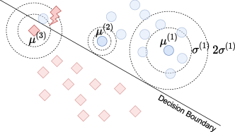
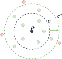
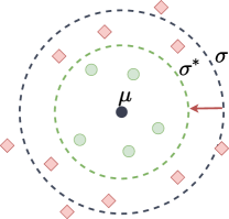
(a)	(b)	(c)

Figure 2: From left to right: (a) Visualization of CVP’s interaction with the decision boundary. (b) A large amount of correctly classified instances will result in a small $\mathcal{L}_{ce}^{\varphi}$ value and therefore an increase of $\sigma$. (c) Likewise, a large amount of incorrect classifications will increase $\mathcal{L}_{ce}^{\varphi}$ and lower the training target $\psi$ and hence also $\sigma$.

3.5 Training Process

Given above formal introduction of our proposed CVP algorithm, we can now describe our full domain adaptation pipeline. Overall, our setup is two-stage with an initial pretraining phase and an iterative domain adaptation refinement step.
Pretraining Phase. Our training setup starts with a pretraining phase. During this phase, only labeled source domain data is used. This phase mainly serves the purpose of initializing the weights of the $f_{\Sigma}$ and $f_{\text{Cl}}$, which can be reliably done with the ground truth source domain annotations. At the end of the pretraining phase, the combination of $f_{\Sigma}(f_{\text{CNN}}(\cdot))$ can already be used to estimate uncertainty while $f_{\text{Cl}}(f_{\text{CNN}}(\cdot))$ can be employed as a pseudo-labeler.
Adaptation Phase. The adaptation phase is an iterative cycle-based refinement step, during which the model is adapted to the target domain. At the start of every adaptation cycle, we utilize the current training progress of our model in order to create pseudo-labels for target domain instances, i.e. we use $\mathit{argmax}\circ f_{\text{Cl}}\circ f_{\text{CNN}}:x_{T}^{(i)}\rightarrow y_{T}^{(i)}$ to generate a label $y_{T}^{(i)}\in\mathcal{C}$ for every target domain instance $x_{T}^{(i)}$. We then follow the procedure of [Ringwald and Stiefelhagen(2020)] and sample mixed domain batches consisting of 50% source domain and 50% target domain images for training. Given such a batch, the model is then optimized w.r.tthe loss function $\mathcal{L}_{\text{total}}$ introduced in section 3.4. This is repeated for $T_{\text{cycle}}$ steps, until the next adaptation cycle begins. The pseudo-label generation always uses the current model weights, therefore only one set of model weights needs to be kept, i.e. no additional memory or storage space is necessary.

4 Experiments

4.1 Evaluation Setup

Datasets. We evaluate our proposed CVP method on four publicly available UDA benchmark datasets: VisDA-2017 (also known as Syn2Real-C) [Peng et al.(2017)Peng, Usman, Kaushik, Hoffman, Wang, and Saenko] is a staple dataset for unsupervised domain adaptation that offers over 200,000 images from 12 object classes in the domains synthetic and real. The synthetic domain (train set) contains 152,397 images of 3D renderings under different lighting conditions and viewing angles. The real domain (test set) contains 72,372 real life images extracted from the YouTube Bounding-Boxes dataset [Real et al.(2017)Real, Shlens, Mazzocchi, Pan, and Vanhoucke]. Adaptiope [Ringwald and Stiefelhagen(2021)] is a very challenging UDA dataset with 123 classes in the three domains synthetic, product and real life. Adaptiope was constructed as a balanced dataset. Therefore, every class and every domain contains the same amount of images, resulting in 36,900 images overall with 100 images per class and 12,300 images per domain. Office-Caltech [Gong et al.(2012)Gong, Shi, Sha, and Grauman] is a common UDA dataset containing 2,533 images of 10 classes in the 4 domains Amazon, Caltech, DSLR and Webcam. Modern Office-31 [Ringwald and Stiefelhagen(2021)] was recently proposed as a replacement for the Office-31 [Saenko et al.(2010)Saenko, Kulis, Fritz, and Darrell] dataset. It rectifies the annotation errors in Office-31 and also adds a new synthetic domain for a total of 6,712 images of 31 classes in the 3 domains Amazon, Webcam and Synthetic. Example images from the datasets are shown in Figure 3.
Evaluation Metrics. For the evaluation of our method, we employ the standard metrics of each dataset: For Adaptiope, we construct six transfer tasks based on the three domains and calculate a mean and standard deviation over multiple runs as proposed in [Ringwald and Stiefelhagen(2021)]. For VisDA-2017, we calculate the mean class accuracy as per challenge evaluation protocol. Here, the standard accuracy is computed per class and then averaged over all 12 classes for a final score. For Modern Office-31 and Office-Caltech, we construct 6 and 12 transfer tasks respectively and report the accuracy per task as well as an overall average. For the evaluation of the decision boundary smoothness, we employ the oscillation of classification metric from [Karimi et al.(2019)Karimi, Derr, and Tang]. Here, we generate subfeatures by linearly interpolating between two features $\mu^{(i)}$ and $\mu^{(j)}$ (denoted as $\mu^{(i,j)}_{k}$ with $k$ being the interpolation step) and measure the number of changes in classification. Formally, we measure $\mathcal{O}(\mu^{(i)},\mu^{(j)})=\frac{1}{K}\sum_{k=1}^{K-1}\mathbf{1}\left(\mathrm{argmax}\;f_{\text{Cl}}(\mu^{(i,j)}_{k})\neq\mathrm{argmax}\;f_{\text{Cl}}(\mu^{(i,j)}_{k+1})\right)$ where $\mathbf{1}$ denotes the indicator function and $K$ is the number of interpolation steps. This metric is visualized in Figure 3c for $K=6$. We provide further information about the implementation details and the evaluation setup in Appendix A.

(a) Adaptiope	(b) VisDA-2017	(c) Boundary smoothness evaluation

Figure 3: (a) Example images from Adaptiope [Ringwald and Stiefelhagen(2021)] with 123 classes in the domains product, real and synthetic. (b) Example images from VisDA-2017 [Peng et al.(2017)Peng, Usman, Kaushik, Hoffman, Wang, and Saenko] with 12 classes in the domains synthetic and real. (c) Visualization of the boundary smoothness evaluation. Top: Interpolating between $\mu^{(i)}$ and $\mu^{(j)}$ results in few class changes due to the smooth decision boundary. Bottom: Interpolating between $\mu^{(m)}$ and $\mu^{(n)}$ results in many changes due to the curvy shape of the boundary.

4.2 Results

Analysis. We start evaluating our CVP method by providing an analysis w.r.tCVP’s $\sigma$ prediction. In Figure 4a and b, we show the batch median $\sigma$ for both source and target domain samples during the adaptation phase as training progresses. During the pretraining phase, the model has only been trained on source domain data. For this reason, a large drop of $\sigma$ can be observed at the beginning of the adaptation phase, as the model is now confronted with target domain data for the first time. The resulting decrease in $\sigma$ can be interpreted as a lower certainty in the model’s predictions due to the involvement of new and unseen data. While the certainty on the source domain quickly recovers, the target domain certainty increase is delayed due to the domain gap and the ongoing domain adaptation during training. For the S$\rightarrow$P task, our CVP model converges to a similar certainty (i.e. magnitude of $\sigma$) for both domains. However, for the hardest transfer task of Adaptiope – S$\rightarrow$R – the mean target domain certainty at the end of training is still lower than the source domain certainty due to the enormous domain gap of synthetic to real transfer tasks.

Furthermore, we analyze $\sigma$ w.r.tcommon uncertainty measures. In total, we compare with five common uncertainty measures: (1) magnitude of the maximum logit ($L$), (2) magnitude of the logit for the ground truth class ($L_{\text{GT}}$), (3) the difference of the top two logits ($L_{\text{diff}}$), (4) the probability at the maximum logit prediction after averaging over multiple Monte Carlo Dropout (MCD) iterations ($MCD_{\mu}$) and (5) the standard deviation at the maximum logit prediction after multiple MCD iterations ($MCD_{\sigma}$, inverted for visualization purposes). We then calculate the Pearson correlation coefficient between $\sigma$ and measure 1-5 and plot the results in Figure 4c for multiple transfer tasks. For all measures we compare with, we observe a strong linear correlation indicating that $\sigma$ can indeed be interpreted as an (un-)certainty measure. This is also consistent for all evaluated transfer tasks.

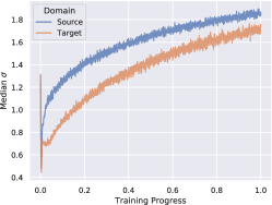
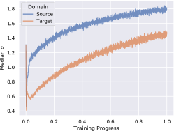
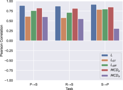
(a) S$\rightarrow$P	(b) S$\rightarrow$R	(c) Correlation

Figure 4: (a, b) Median $\sigma$ values for the source and target domain as the training progresses. (c) Correlation of $\sigma$ with common uncertainty measures. Best viewed in the digital version.

Metric	Setup	Losses	P$\rightarrow$S	R$\rightarrow$S	S$\rightarrow$P	S$\rightarrow$R	Avg.
Accuracy	Basic	$\mathcal{L}^{\mu}_{\text{ce}}$	69.4	70.1	74.8	60.0	68.6
	No Samples CE	$\mathcal{L}^{\mu}_{\text{ce}},\mathcal{L}_{\text{ant}}$	70.7	70.8	77.1	61.9	70.1
	Full CVP Setup	$\mathcal{L}^{\mu}_{\text{ce}},\mathcal{L}_{\text{ant}},\mathcal{L}^{\varphi}_{\text{ce}}$	71.9	72.4	78.4	63.2	71.5
Oscillation	Basic	$\mathcal{L}^{\mu}_{\text{ce}}$	205.9$\pm$1.3	207.2$\pm$0.2	221.2$\pm$3.8	259.6$\pm$2.7	223.5
	Full CVP Setup	$\mathcal{L}^{\mu}_{\text{ce}},\mathcal{L}_{\text{ant}},\mathcal{L}^{\varphi}_{\text{ce}}$	197.1$\pm$0.6	199.3$\pm$1.2	208.9$\pm$1.6	233.0$\pm$4.8	209.6

Table 1: Effect of CVP on the classification results and the smoothness of the decision boundary quantified by the oscillation of classification metric. Results are given as accuracy (in %, $\uparrow$ higher is better) and osciallation of classification metric $\mathcal{O}(\cdot,\cdot)$ summed over all sampled feature pairs ($\downarrow$ lower is better).

We also conduct an ablation study w.r.tour model’s three loss functions and show results in Table 1 for the four difficult transfer tasks involving Adaptiope’s synthetic domain. In the basic setup, only $\mathcal{L}^{\mu}_{\text{ce}}$ is used. This is the minimal setup in order to train the classifier and obtain pseudo-labels. As expected, this performs the worst of all evaluated setups, as CVP’s additional loss functions are not active. We continue by adding $\mathcal{L}_{\text{ant}}$. This already improves the classification accuracy for all four transfer tasks. However, without the $\mathcal{L}^{\varphi}_{\text{ce}}$ loss, the cluster assumption is not enforced, which yields excessive $\sigma$ values and results in lower accuracies than our full CVP method. Only the usage of all three losses – $\mathcal{L}^{\mu}_{\text{ce}}$, $\mathcal{L}^{\varphi}_{\text{ce}}$ and $\mathcal{L}_{\text{ant}}$ – results in the highest accuracy for all four transfer tasks with an average improvement of almost 3% over the basic setup. Note that training with $\mathcal{L}^{\varphi}_{\text{ce}}$ but without $\mathcal{L}_{\text{ant}}$ would instantly collapse $\sigma$ towards 0 and break the feature sampling due to the zero standard deviation. We thus do not show results for this setup. This is further discussed in Section 3.4.

Finally, we analyze the smoothness of the decision boundary. For this analysis, we employ the osciallation of classification metric described in Section 4.1. After the conclusion of CVP’s adaptation phase, we extract features $\mu$ for five instances per class and then calculate the sum of this metric for all distinct pairs $(i,j)$, i.e. $\sum_{i}\sum_{j}\mathcal{O}(\mu^{(i)},\mu^{(j)})$. The results are shown in Table 1 as mean and standard deviation over multiple runs. Applying CVP clearly leads to a much smoother decision boundary as quantified by the oscillation metric. For every analysed transfer task, the setup using CVP has a multiple standard deviations lower oscillation value, which is a direct indication of a smoother decision boundary. Overall, applying CVP results in an approximately 14 points lower oscillation metric, which translates to 14,000 fewer changes in classification. Smoothness of the decision boundary is also strong indicator for the generalization capabilities of a model. This is especially important in UDA, as the trained model is employed as pseudo-labeler for subsequent training steps – a better generalization would necessarily lead to better pseudo-labels $y_{T}^{(i)}$. We therefore also provide domain adaptation results with and without CVP in Table 1. We observe that every model employing CVP improves in accuracy on the target domain when compared to a model without CVP. On average, CVP improves the domain adaptation results by 2.9%, with a 3.2% increase on the hardest transfer task S$\rightarrow$R and up to 3.6% on S$\rightarrow$P. We thus conclude that CVP can be seen as an intuitive uncertainty measure that improves domain adaptation capabilities by smoothing the decision boundary of a classifier. For further ablation studies, please refer to Appendix C.

Method aero bicyc bus car horse knife motor person plant skate train truck Avg. Source only 56.0 15.3 63.4 95.3 62.0 18.4 70.2 26.2 89.1 26.0 88.6 13.2 52.0 SE-152 [French et al.(2018)French, Mackiewicz, and Fisher] 88.4 84.8 75.1 84.1 80.0 72.6 63.6 56.6 95.4 73.8 77.6 78.3 77.5 BUPT [Peng et al.(2017)Peng, Usman, Kaushik, Hoffman, Wang, and Saenko] 95.7 67.0 93.4 97.2 90.6 86.9 92.0 74.2 96.3 66.9 95.2 69.2 85.4 CAN [Kang et al.(2019)Kang, Jiang, Yang, and Hauptmann] — — — — — — — — — — — — 87.4 SDAN [G. Csurka and Clinchant(2020)] 94.3 86.5 86.9 95.1 91.1 90.0 82.1 77.9 96.4 77.2 86.6 88.0 87.7 UFAL [Ringwald and Stiefelhagen(2020)] 94.9 87.0 87.0 96.5 91.8 95.1 76.8 78.9 96.5 80.7 93.6 86.5 88.8 CVP (ours) 95.2 89.1 91.2 94.6 92.4 91.3 82.2 78.4 96.6 87.9 91.3 90.5 90.1

Table 2: Per class accuracy (in %) for different methods on the VisDA-2017 test set as per challenge evaluation protocol. The domains are synthetic (source) and real (target).

Method	P$\rightarrow$R	P$\rightarrow$S	R$\rightarrow$P	R$\rightarrow$S	S$\rightarrow$P	S$\rightarrow$R	Avg.
Source only	60.6$\pm$1.2	28.7$\pm$1.6	76.9$\pm$0.4	26.9$\pm$1.1	21.2$\pm$2.4	8.8$\pm$4.6	37.2
RSDA-DANN [Gu et al.(2020)Gu, Sun, and Xu, Ganin and Lempitsky(2015)]	78.6$\pm$0.1	48.5$\pm$0.7	90.0$\pm$0.0	43.9$\pm$0.9	63.2$\pm$1.1	37.0$\pm$1.2	60.2
RSDA-MSTN [Gu et al.(2020)Gu, Sun, and Xu, Xie et al.(2018)Xie, Zheng, Chen, and Chen]	73.8$\pm$0.2	59.2$\pm$0.2	87.5$\pm$0.2	50.3$\pm$0.5	69.5$\pm$0.6	44.6$\pm$1.1	64.2
SymNets [Zhang et al.(2019)Zhang, Tang, Jia, and Tan]	81.4$\pm$0.3	53.1$\pm$0.6	92.3$\pm$0.2	49.2$\pm$1.0	69.6$\pm$0.5	44.9$\pm$1.5	65.1
CAN [Kang et al.(2019)Kang, Jiang, Yang, and Hauptmann]	81.5$\pm$0.3	72.3$\pm$0.3	92.2$\pm$0.2	69.3$\pm$0.9	74.9$\pm$1.1	60.7$\pm$0.6	75.2
CVP (ours)	81.7$\pm$0.1	71.6$\pm$0.4	91.5$\pm$0.1	71.8$\pm$0.8	77.2$\pm$1.7	62.3$\pm$1.3	76.0

Table 3: Classification accuracy (in %) for the Adaptiope dataset using a ResNet-50 backbone architecture. The domains are synthetic (S), real (R) and product (P).

Comparison to State-of-the-Art. We now compare our proposed CVP algorithm to recently proposed unsupervised domain adaptation methods. On the VisDA-2017 dataset (see Table 2), CVP is able to outperform recent methods and achieves the best accuracy for 5 out of 12 classes and improves the mean class average by 1.3% w.r.tto the previous SOTA result. To the best of our knowledge, this poses the best published result for the commonly used ResNet-101 backbone. Given the current VisDA-2017 challenge leaderboard [Kate Saenko and Peng(2017)], our CVP method would rank 2^nd place – only behind a much larger $5\times$ResNet-152 ensemble that also averages results over multiple runs with test time augmentations. This, however, is not a fair comparison to our single ResNet-101 setup without such test time tricks.
On the Adaptiope dataset (see Table 3), we compare to the recent CVPR proposals SymNets [Zhang et al.(2019)Zhang, Tang, Jia, and Tan], CAN [Kang et al.(2019)Kang, Jiang, Yang, and Hauptmann] and RSDA [Gu et al.(2020)Gu, Sun, and Xu] (using both DANN [Ganin and Lempitsky(2015)] and MSTN [Xie et al.(2018)Xie, Zheng, Chen, and Chen]). Again, CVP is able to surpass these state-of-the-art algorithms and achieves the best accuracy on 4 out of 6 transfer tasks and also the overall average. Even for the hardest transfer tasks – i.e. those involving synthetic images as source domain – CVP manages to improve the results of CAN [Kang et al.(2019)Kang, Jiang, Yang, and Hauptmann] by 1.6% for S$\rightarrow$R and 2.3% for S$\rightarrow$P. Again, CVP’s overall accuracy average of 76% poses the best published result and shows that our method can reliably conduct domain adaptation, even when confronted with Adaptiope’s 123 difficult classes.
Furthermore, we report results on the Office-Caltech dataset in Table 4. Again, our CVP method is able to achieve the best or second best results in 9 out of 12 transfer tasks and is also within 0.6% of UFAL [Ringwald and Stiefelhagen(2020)]. Please note that due to Office-Caltech’s average target domain size of only 633 images, a 0.6% difference arises from less than 2 misclassifications per transfer task on average. Therefore, our CVP method can be considered on par with the top performing methods UFAL [Ringwald and Stiefelhagen(2020)], PrDA [Hua and Guo(2020)] and RWA [van Laarhoven and Marchiori(2017)].
Finally, we report results on the Modern Office-31 dataset in Table 5. Yet again, CVP is able to achieve the best or second best result in 4 out of the 6 available transfer tasks and is on par with the recently proposed RSDA [Gu et al.(2020)Gu, Sun, and Xu] and CAN [Kang et al.(2019)Kang, Jiang, Yang, and Hauptmann] methods. For the difficult A_ref$\rightarrow$S task, CVP even manages to improve upon prior methods by 2.0%. We thus conclude that CVP is able to successfully conduct unsupervised domain adaptation on a wide variety of transfer tasks and datasets and is able to achieve results at or close to state-of-the-art level.

Method	A			C			D			W			Avg.
	C	D	W	A	D	W	A	C	W	A	C	D
CORAL [Sun et al.(2016)Sun, Feng, and Saenko, van Laarhoven and Marchiori(2017)]	89.2	92.2	91.9	94.1	92.0	92.1	94.3	87.7	98.0	92.8	86.7	100.0	92.6
GTDA+LR [Vascon et al.(2019)Vascon, Aslan, Torcinovich, van Laarhoven, Marchiori, and Pelillo]	91.5	98.7	94.2	95.4	98.7	89.8	95.2	89.0	99.3	95.2	90.4	100.0	94.8
RWA [van Laarhoven and Marchiori(2017)]	93.8	98.9	97.8	95.3	99.4	95.9	95.8	93.1	98.4	95.3	92.4	99.2	96.3
PrDA [Hua and Guo(2020)]	92.1	99.0	99.3	97.2	99.4	98.3	94.7	91.0	99.7	95.6	93.4	100.0	96.6
UFAL [Ringwald and Stiefelhagen(2020)]	95.1	99.4	99.7	96.0	96.8	99.7	95.8	95.0	99.7	96.3	95.0	99.4	97.3
CVP (ours)	94.3	98.1	99.0	96.6	91.7	98.3	95.9	94.7	100.0	96.1	95.3	100.0	96.7

Table 4: Classification accuracy (in %) for different methods using ResNet-50 on the Office-Caltech dataset with domains Amazon, Caltech, DSLR and Webcam.

Method	Aref$\rightarrow$S	Aref$\rightarrow$W	W$\rightarrow$Aref	W$\rightarrow$S	S$\rightarrow$Aref	S$\rightarrow$W	Avg.
Source only [Ringwald and Stiefelhagen(2021)]	51.3	76.8	74.1	51.3	14.9	8.0	46.1
SymNet [Zhang et al.(2019)Zhang, Tang, Jia, and Tan]	65.9	91.0	89.2	56.5	86.8	82.2	78.6
RSDA-DANN [Gu et al.(2020)Gu, Sun, and Xu, Ganin and Lempitsky(2015)]	76.1	91.8	90.5	70.4	80.8	83.1	82.1
RSDA-MSTN [Gu et al.(2020)Gu, Sun, and Xu, Xie et al.(2018)Xie, Zheng, Chen, and Chen]	82.0	92.2	93.0	76.3	90.0	86.2	86.6
CAN [Kang et al.(2019)Kang, Jiang, Yang, and Hauptmann]	79.1	92.8	90.9	77.9	91.2	89.7	86.9
CVP (ours)	84.0	91.4	91.1	77.5	90.4	85.2	86.6

Table 5: Classification accuracy (in %) on the Modern Office-31 dataset using ResNet-50.

5 Conclusion

In this paper, we propose CVP – the Certainty Volume Prediction algorithm – for estimation of uncertainty in feature space. We show how CVP’s sampling stage interacts with the decision boundary and how this can improve a model’s generalization properties and therefore domain adaptation capabilities. Additionally, we show that CVP’s $\sigma$ estimation in feature space relates to other common uncertainty quantifications in classifier space. Due to the intuitive interpretability of $\sigma$, we also see great potential for other downstream tasks, e.gemploying $\sigma$ for out-of-distribution rejection in open-set domain adaptation. Overall, we demonstrate that making a model uncertainty-aware through CVP can improve its predictions and achieve state-of-the-art results on challenging benchmark UDA datasets.

Appendices

Appendix A Implementation Details

In this section, we provide further detail about the employed setup and evaluation. For our experiments on VisDA-2017 [Peng et al.(2017)Peng, Usman, Kaushik, Hoffman, Wang, and Saenko], we employ the common ResNet-101 [He et al.(2016)He, Zhang, Ren, and Sun] feature extractor ($f_{\text{CNN}}$) similar to [Kang et al.(2019)Kang, Jiang, Yang, and Hauptmann, French et al.(2018)French, Mackiewicz, and Fisher, Ringwald and Stiefelhagen(2020)], while for Office-Caltech [Gong et al.(2012)Gong, Shi, Sha, and Grauman], Modern Office-31 [Ringwald and Stiefelhagen(2021)] and Adaptiope [Ringwald and Stiefelhagen(2021)], we use ResNet-50 as proposed in [Ringwald and Stiefelhagen(2021)]. In all cases, $f_{\text{CNN}}$ is pretrained on ImageNet [Deng et al.(2009)Deng, Dong, Socher, Li, Li, and Fei-Fei]. We implement the $f_{\Sigma}$ subnetwork as a two layer linear network. The input size is 2048 (same size as $\mu$), hidden size 2048 and output size 1. Intermediate outputs are activated by ReLU. The final output is activated by the softplus function in order to enforce $\sigma\in\mathbb{R}^{+}_{0}$ and the positive semi-definiteness of $\Sigma$.
We jointly optimize all parameters using SGD with Nesterov momentum [Nesterov(1983)] of 0.95 and a learning rate of $5\times 10^{-4}$, which is decreased according to the schedule used in [Kang et al.(2019)Kang, Jiang, Yang, and Hauptmann]. Networks are trained for 250 cycles with $T_{\text{cycle}}=50$ forward passes each. For the evaluation of the decision boundary, we set $K=1000$ in order to sample 1000 subfeatures (including start and end feature). Our code is implemented in PyTorch [Paszke et al.(2017)Paszke, Gross, Chintala, et al.] and will be made available.
Reparameterization Trick. Neural network training is based on the idea of backpropagation and therefore requires the whole network to be differentiable. This, however, is not the case when including a generally non-differentiable step such as sampling from a distribution. In this work, we want the parameters of $f_{\Sigma}$ to also be updated based on our proposed $\mathcal{L}_{\text{ce}}^{\varphi}$ loss function. We thus sidestep the non-differentiability of sampling by applying the reparameterization trick proposed in [Kingma and Welling(2013)]. Here, instead of sampling a feature $z$ directly from $z\sim\mathcal{N}(\mu,\Sigma)$, we first draw an auxiliary noise variable $\varepsilon\sim\mathcal{N}(\mathbb{0},\mathbb{1})$ and then compute $z=\mu+\varepsilon\Sigma^{\frac{1}{2}}$. This can also be rewritten as $\forall i:z_{i}=\mu_{i}+\varepsilon_{i}\;\mathrm{diag}(\Sigma^{\frac{1}{2}})_{i}$ with $\varepsilon_{i}\sim\mathcal{N}(0,1)$ (note the scalar notation). Applying this reparameterization allows the gradient to also flow through our $f_{\Sigma}$ subnetwork.

Appendix B Theorem for $\kappa$ Initialization

We now derive the constant $\kappa$ (used in the $\psi^{(i)}$ equation in the main paper) as the expected cross-entropy value given a randomly initialized classifier. Consider the cross-entropy term $H(q,p)=-\sum q\;\mathrm{log}(p)$ between two categorical distributions $q$ and $p$ with $\lvert\mathcal{C}\rvert$ classes. Given an uniform class distribution, the one-hot encoded target $q_{i}$ will equal 1 at position $i$ with probability $\frac{1}{\lvert\mathcal{C}\rvert}$. We can then rewrite $H(q,p)=-\sum_{i=1}^{\lvert\mathcal{C}\rvert}\frac{1}{\lvert\mathcal{C}\rvert}\;\mathrm{log}(p_{i})$. This can be further simplified as Equation 4.

$$H(q,p)=-\frac{1}{\lvert\mathcal{C}\rvert}\sum_{i=1}^{\lvert\mathcal{C}\rvert}\mathrm{log}(p_{i})=-\frac{1}{C}(\mathrm{log}(p_{1})+...+\mathrm{log}(p_{\lvert\mathcal{C}\rvert}))=-\frac{1}{\lvert\mathcal{C}\rvert}\mathrm{log}(p_{1}\cdot p_{2}\ldots\cdot p_{\lvert\mathcal{C}\rvert})$$ (4)

We can assume that the worst state of a model during training is to be equal to a random oracle, i.e. we assume that $\forall i:\mathbb{E}[p_{i}]\approx\frac{1}{\lvert\mathcal{C}\rvert}$ holds true. Given this assumption, we can rewrite Equation 4 as $H(q,p)=-\frac{1}{\lvert\mathcal{C}\rvert}\mathrm{log}(\frac{1}{\lvert\mathcal{C}\rvert}^{\lvert\mathcal{C}\rvert})=-\frac{\lvert\mathcal{C}\rvert}{\lvert\mathcal{C}\rvert}\mathrm{log}(\frac{1}{\lvert\mathcal{C}\rvert})=-\mathrm{log}(\frac{1}{\lvert\mathcal{C}\rvert})$, which further simplifies to $\mathrm{log}(\lvert\mathcal{C}\rvert)$. We thus define constant $\kappa=\mathrm{log}(\lvert\mathcal{C}\rvert)$, which can be seen as an expected upper bound for $\mathcal{L}_{ce}^{\varphi}$.

Appendix C Additional Analysis

Ablation Study. We also evaluate our proposed CVP method by conducting an ablation study w.r.tits two hyperparameters $\alpha$ and $M$. For this evaluation, we use Adaptiope’s S$\rightarrow$P and S$\rightarrow$R transfer tasks. Hyperparameter $M$ controls the amount of samples that are drawn from the distribution predicted by CVP. We analyze $M$ in the range $[2^{5},2^{8}]$ and plot the results in Figure Ia. We notice that CVP is fairly robust w.r.tto this parameter as long as enough samples are drawn. Overall $M=2^{6}$ resulted in the best performance. Similarly, we analyze the samples weight $\alpha$ in Figure Ib. We observe that choosing $\alpha$ either to low or too high degrades the accuracy consistently for both transfer tasks. Intuitively, a too high $\alpha$ would attribute the generated samples the same weight as the predicted mean feature $\mu$, which can lead to optimization problems, as the samples are randomly drawn and not an actual output of the feature extractor. Related to this, setting $\alpha$ too low removes the additional supervision to enforce the cluster assumption. We thus set $\alpha=0.5$ for our experiments, due to its overall best performance.
Sigma Analysis. Furthermore, we provide an additional analysis for the P$\rightarrow$S task of Adaptiope similar to the analysis in the main paper in Figure Ic. We note the same key observations as for the S$\rightarrow$P and S$\rightarrow$R tasks in the main paper: Directly after the switch from the pretraining to the adaptation phase, $\sigma$ drops harshly due to being confronted with new, unseen target domain data. For the source domain, $\sigma$ recovers quickly while for the target domain, $\sigma$ grows slower due to the ongoing domain adaptation. Unlike the S$\rightarrow\ast$ tasks, the source and target domain $\sigma$ end up very close to each other for the S$\rightarrow$P task. This, however, is expected due to the smaller domain gap and the missing background clutter: both the synthetic and the product domain have cropped items with either a fully white (product domain) or fully grey (synthetic domain) background.
Interpretability of $\sigma$. We further analyze the interpretability of $\sigma$. For this, we run our full CVP method on Adaptiope’s S$\rightarrow$R task and extract $\sigma$ values for the whole target domain. In Figure II, we show selected results from the top and bottom 20 $\sigma$ values. Images associated with high magnitudes of $\sigma$ are usually taken under good conditions w.r.tlighting and camera angle and commonly represent the best images of their respective object classes. For low magnitudes of $\sigma$, we often find objects to be in unusual positions (see Figure IId), disassembled or broken (see Figure IIa) or in exceptionally uncommon conditions or situations (see Figure IIe). This further reinforces the usability of $\sigma$ as an interpretable uncertainty measure.

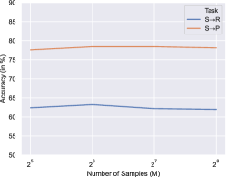
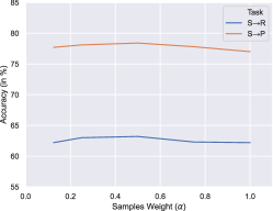
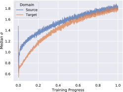
(a) Number of Samples $M$	(b) Samples Weight $\alpha$	(c) P$\rightarrow$S

Figure I: (a, b) Results for different ablation studies. (c) Median $\sigma$ values for the source and target domain as the training progresses. Best viewed in the digital version.

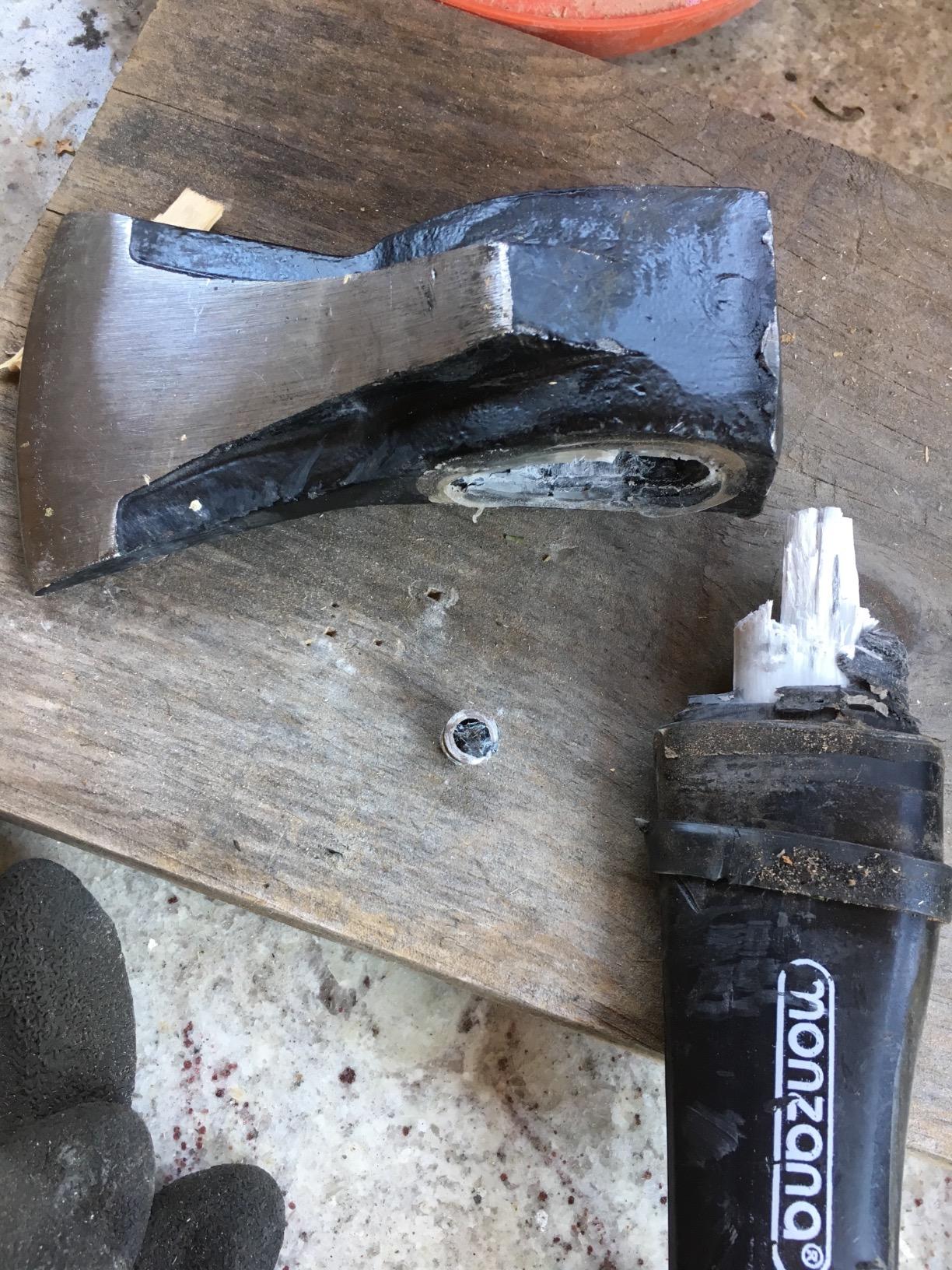
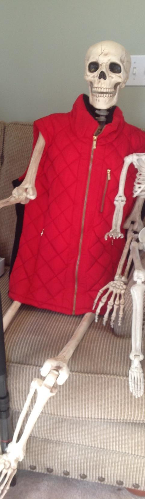
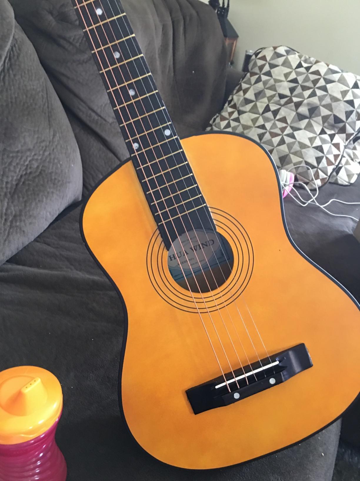
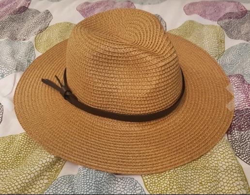
(a) axe				(b) acoustic guitar	(c) hat
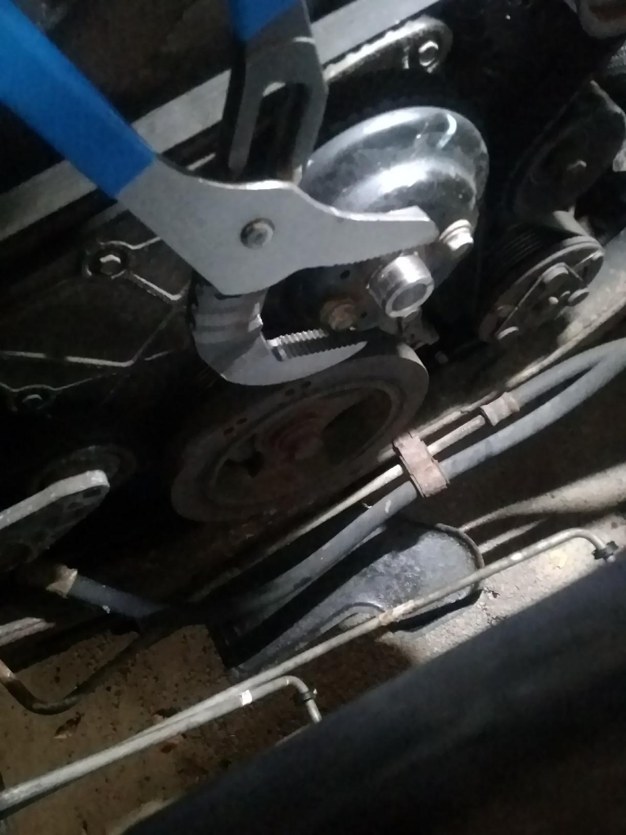
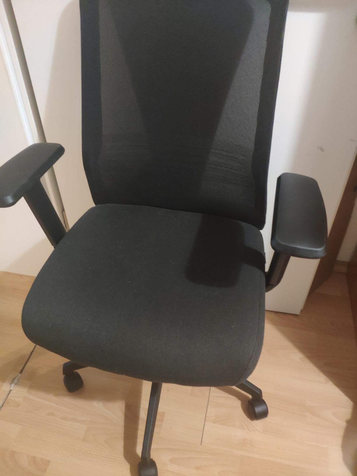
(d) pipe wrench	(e) skeleton			(f) office chair	(g) tent
Low $\sigma$ magnitude			High $\sigma$ magnitude

Figure II: Left two columns: Images associated with a low magnitude of $\sigma$. Right two columns: Images associated with high magnitudes of $\sigma$. Image captions denote the ground truth class.

Appendix D Visualization

In Figure III, we provide a feature visualization for the features learned by our CVP method. For this, we extract the 2048-dimensional feature $\mu$ for every target domain image in Adaptiope’s S$\rightarrow$P and S$\rightarrow$R transfer tasks respectively. The feature extraction step is conducted right after the source-only pretraining and after the finalized domain adaptation phase. We then employ t-SNE [Maaten and Hinton(2008)] in order to project the features into a two-dimensional space. As evident from Figure IIIa, the features show no discernible structure with regard to clusters or proximity of same-class features after the source-only pretraining step. However, after the adaptation phase with CVP (Figure IIIb), clear clusters of same-class features can be observed. We thus conclude that – even for the very hard synthetic to real and synthetic to product transfer tasks of Adaptiope – our CVP method was able to learn discriminative features even though no target domain labels were available.

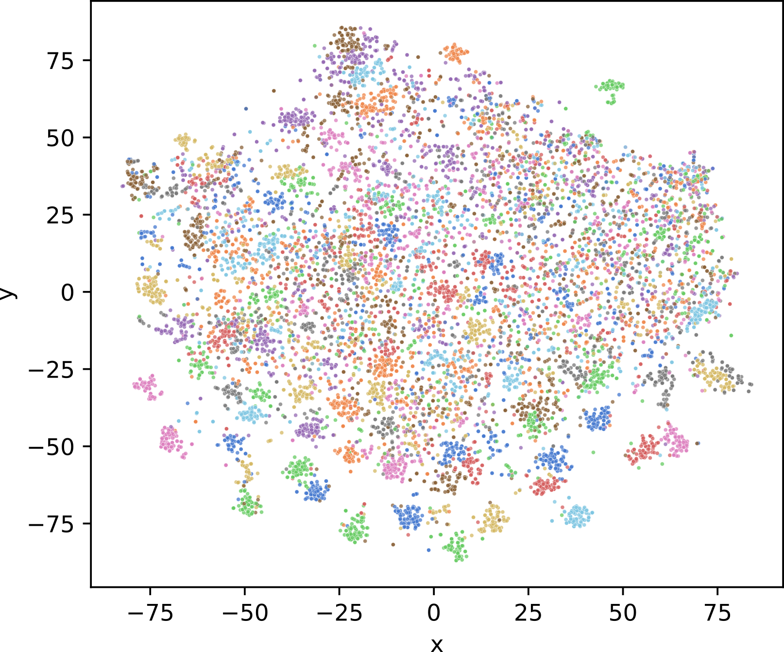
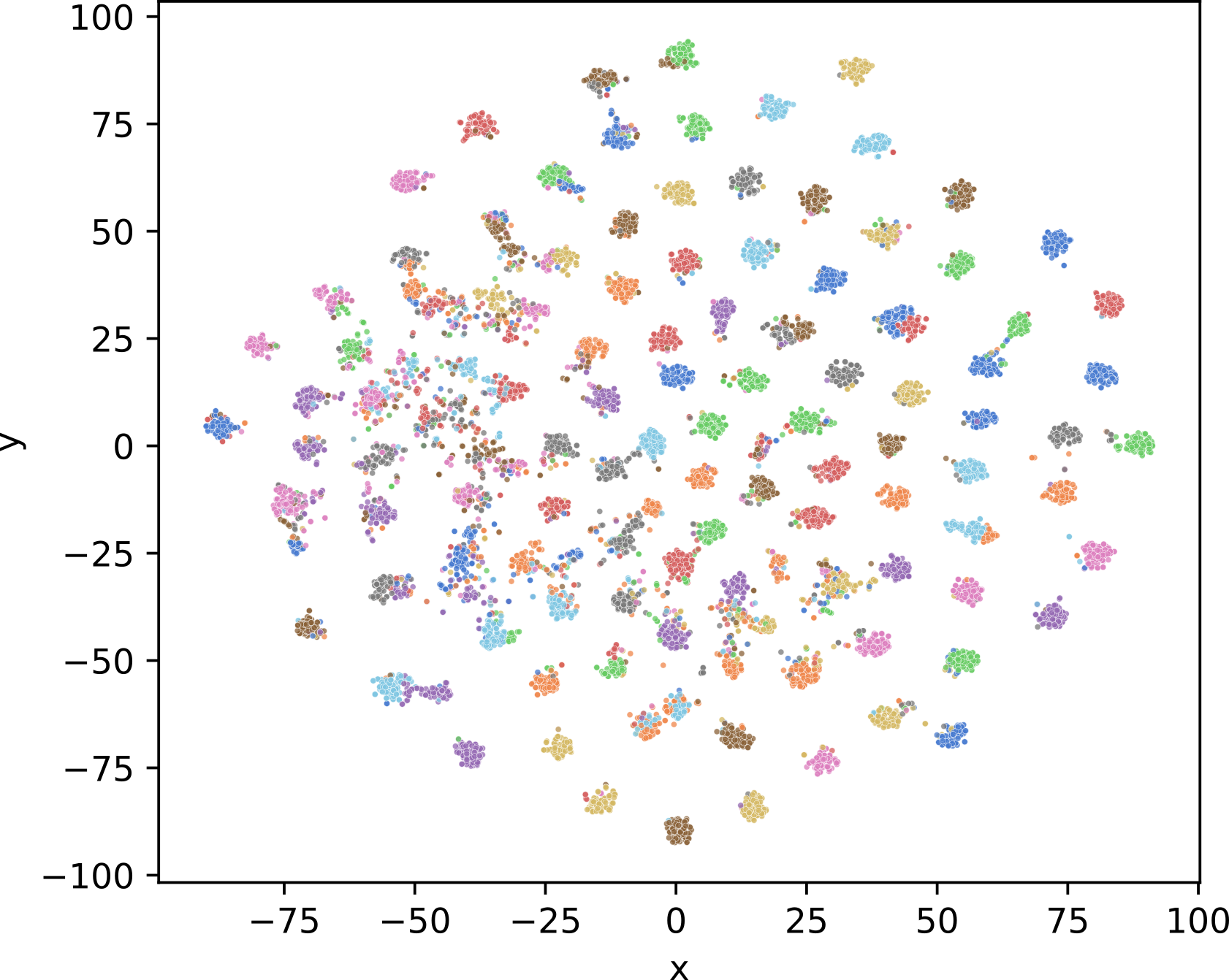
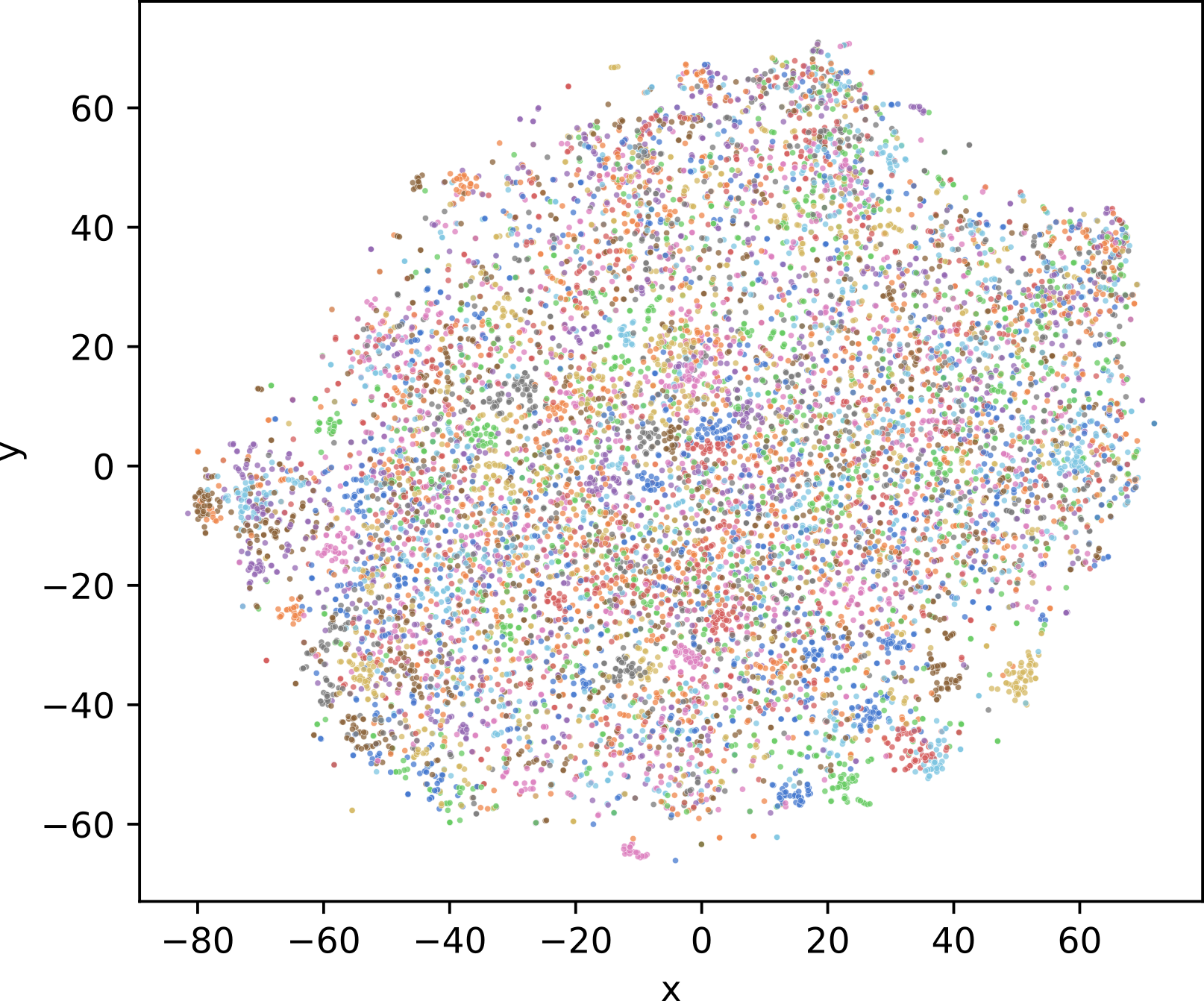
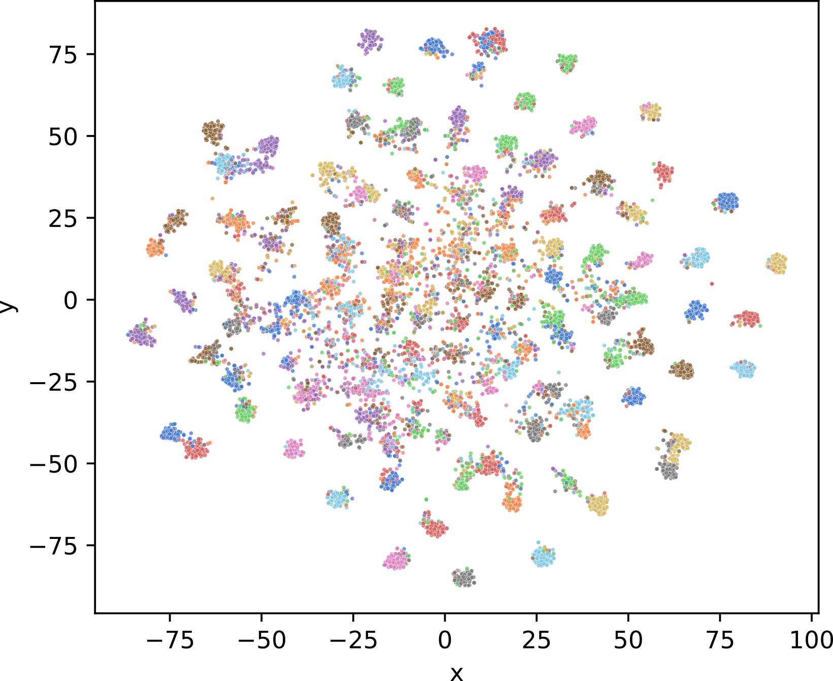
(a) After Pretraining	(b) After Adaptation

Figure III: Visualization of target domain features after the source-only pretraining and after the domain adaptation with CVP. Features were extracted for Adaptiope’s S$\rightarrow$P (top row) and S$\rightarrow$R (bottom row) transfer tasks. Every color represents one of Adaptiope’s 123 classes. Please note that due to the high number of classes, some colors are hard to distinguish.

References

- [Atapour-Abarghouei and Breckon(2018)] Amir Atapour-Abarghouei and Toby P Breckon. Real-time monocular depth estimation using synthetic data with domain adaptation via image style transfer. In Proceedings of the IEEE Conference on Computer Vision and Pattern Recognition, pages 2800–2810, 2018.
- [Bartlett and Shawe-taylor(1998)] Peter Bartlett and John Shawe-taylor. Generalization performance of support vector machines and other pattern classifiers, 1998.
- [Chang et al.(2019)Chang, You, Seo, Kwak, and Han] Woong-Gi Chang, Tackgeun You, Seonguk Seo, Suha Kwak, and Bohyung Han. Domain-specific batch normalization for unsupervised domain adaptation. In Proceedings of the IEEE Conference on Computer Vision and Pattern Recognition, pages 7354–7362, 2019.
- [Chapelle and Zien(2005)] Olivier Chapelle and Alexander Zien. Semi-supervised classification by low density separation. In AISTATS, volume 2005, pages 57–64. Citeseer, 2005.
- [Deng et al.(2009)Deng, Dong, Socher, Li, Li, and Fei-Fei] Jia Deng, Wei Dong, Richard Socher, Li-Jia Li, Kai Li, and Li Fei-Fei. Imagenet: A large-scale hierarchical image database. In 2009 IEEE conference on computer vision and pattern recognition, pages 248–255. Ieee, 2009.
- [French et al.(2018)French, Mackiewicz, and Fisher] Geoff French, Michal Mackiewicz, and Mark Fisher. Self-ensembling for visual domain adaptation. In International Conference on Learning Representations, 2018. URL https://openreview.net/forum?id=rkpoTaxA-.
- [G. Csurka and Clinchant(2020)] B. Chidlovskii G. Csurka and S. Clinchant. VisDA Classification Challenge:Runner-Up Talk. https://ai.bu.edu/visda-2017/assets/attachments/VisDA_NaverLabs.pdf, 2020. Accessed: 2020-03-31.
- [Gal and Ghahramani(2016)] Yarin Gal and Zoubin Ghahramani. Dropout as a bayesian approximation: Representing model uncertainty in deep learning. In international conference on machine learning, pages 1050–1059, 2016.
- [Ganin and Lempitsky(2015)] Yaroslav Ganin and Victor Lempitsky. Unsupervised domain adaptation by backpropagation. In Proceedings of the 32Nd International Conference on International Conference on Machine Learning - Volume 37, ICML’15, pages 1180–1189. JMLR.org, 2015. URL http://dl.acm.org/citation.cfm?id=3045118.3045244.
- [Gholami et al.(2017)Gholami, Pavlovic, et al.] Behnam Gholami, Vladimir Pavlovic, et al. Punda: Probabilistic unsupervised domain adaptation for knowledge transfer across visual categories. In Proceedings of the IEEE International Conference on Computer Vision, pages 3581–3590, 2017.
- [Gong et al.(2012)Gong, Shi, Sha, and Grauman] Boqing Gong, Yuan Shi, Fei Sha, and Kristen Grauman. Geodesic flow kernel for unsupervised domain adaptation. In 2012 IEEE Conference on Computer Vision and Pattern Recognition, pages 2066–2073. IEEE, 2012.
- [Goodfellow et al.(2014)Goodfellow, Pouget-Abadie, Mirza, Xu, Warde-Farley, Ozair, Courville, and Bengio] Ian J Goodfellow, Jean Pouget-Abadie, Mehdi Mirza, Bing Xu, David Warde-Farley, Sherjil Ozair, Aaron Courville, and Yoshua Bengio. Generative adversarial nets. In Advances in neural information processing systems, page 2672–2680, 2014.
- [Gretton et al.(2006)Gretton, Borgwardt, Rasch, Schölkopf, and Smola] Arthur Gretton, Karsten Borgwardt, Malte Rasch, Bernhard Schölkopf, and Alex Smola. A kernel method for the two-sample-problem. Advances in neural information processing systems, 19:513–520, 2006.
- [Gu et al.(2020)Gu, Sun, and Xu] Xiang Gu, Jian Sun, and Zongben Xu. Spherical space domain adaptation with robust pseudo-label loss. In Proceedings of the IEEE/CVF Conference on Computer Vision and Pattern Recognition, pages 9101–9110, 2020.
- [Guan et al.(2021)Guan, Huang, Xiao, Lu, and Cao] Dayan Guan, Jiaxing Huang, Aoran Xiao, Shijian Lu, and Yanpeng Cao. Uncertainty-aware unsupervised domain adaptation in object detection. IEEE Transactions on Multimedia, 2021.
- [Han et al.(2019)Han, Zou, Gao, Wang, and Metaxas] Ligong Han, Yang Zou, Ruijiang Gao, Lezi Wang, and Dimitris Metaxas. Unsupervised domain adaptation via calibrating uncertainties. In CVPR Workshops, volume 9, 2019.
- [He et al.(2016)He, Zhang, Ren, and Sun] Kaiming He, Xiangyu Zhang, Shaoqing Ren, and Jian Sun. Deep residual learning for image recognition. In Proceedings of the IEEE conference on computer vision and pattern recognition, pages 770–778, 2016.
- [Hindi and Al-Akhras(2011)] K. E. Hindi and M. Al-Akhras. Smoothing decision boundaries to avoid overfitting in neural network training. Neural Network World, 21:311–325, 2011.
- [Hoffman et al.(2018)Hoffman, Tzeng, Park, Zhu, Isola, Saenko, Efros, and Darrell] Judy Hoffman, Eric Tzeng, Taesung Park, Jun-Yan Zhu, Phillip Isola, Kate Saenko, Alexei A. Efros, and Trevor Darrell. Cycada: Cycle consistent adversarial domain adaptation. In International Conference on Machine Learning (ICML), 2018.
- [Hua and Guo(2020)] Kevin Hua and Yuhong Guo. Unsupervised domain adaptation with progressive domain augmentation. arXiv preprint arXiv:2004.01735, 2020.
- [Kang et al.(2019)Kang, Jiang, Yang, and Hauptmann] Guoliang Kang, Lu Jiang, Yi Yang, and Alexander G Hauptmann. Contrastive adaptation network for unsupervised domain adaptation. In Proceedings of the IEEE Conference on Computer Vision and Pattern Recognition, pages 4893–4902, 2019.
- [Karimi et al.(2019)Karimi, Derr, and Tang] Hamid Karimi, Tyler Derr, and Jiliang Tang. Characterizing the decision boundary of deep neural networks. arXiv preprint arXiv:1912.11460, 2019.
- [Kate Saenko and Peng(2017)] Ben Usman Kate Saenko and Xingchao Peng. 2017 Visual Domain Adaptation (VisDA2017) Classification Challenge . https://competitions.codalab.org/competitions/17052, 2017. Accessed: 2021-04-06.
- [Kingma and Welling(2013)] Diederik P Kingma and Max Welling. Auto-encoding variational bayes. arXiv preprint arXiv:1312.6114, 2013.
- [Lee et al.(1995)Lee, Bartlett, and Williamson] Wee Sun Lee, Peter L Bartlett, and Robert C Williamson. Lower bounds on the vc dimension of smoothly parameterized function classes. Neural Computation, 7(5):1040–1053, 1995.
- [Long et al.(2013)Long, Wang, Ding, Sun, and Yu] Mingsheng Long, Jianmin Wang, Guiguang Ding, Jiaguang Sun, and Philip S Yu. Transfer feature learning with joint distribution adaptation. In Proceedings of the IEEE international conference on computer vision, pages 2200–2207, 2013.
- [Maaten and Hinton(2008)] Laurens van der Maaten and Geoffrey Hinton. Visualizing data using t-sne. Journal of machine learning research, 9(Nov):2579–2605, 2008.
- [Meng et al.(2018)Meng, Li, Gong, and Juang] Zhong Meng, Jinyu Li, Yifan Gong, and Biing-Hwang Juang. Adversarial teacher-student learning for unsupervised domain adaptation. In 2018 IEEE International Conference on Acoustics, Speech and Signal Processing (ICASSP), pages 5949–5953. IEEE, 2018.
- [Murez et al.(2018)Murez, Kolouri, Kriegman, Ramamoorthi, and Kim] Zak Murez, Soheil Kolouri, David Kriegman, Ravi Ramamoorthi, and Kyungnam Kim. Image to image translation for domain adaptation. In Proceedings of the IEEE Conference on Computer Vision and Pattern Recognition, pages 4500–4509, 2018.
- [Nesterov(1983)] Yurii E Nesterov. A method for solving the convex programming problem with convergence rate o (1/k^ 2). In Dokl. akad. nauk Sssr, volume 269, pages 543–547, 1983.
- [Park et al.(2018)Park, Park, Shin, and Moon] Sungrae Park, JunKeon Park, Su-Jin Shin, and Il-Chul Moon. Adversarial dropout for supervised and semi-supervised learning. In Thirty-Second AAAI Conference on Artificial Intelligence, 2018.
- [Paszke et al.(2017)Paszke, Gross, Chintala, et al.] Adam Paszke, Sam Gross, Soumith Chintala, et al. Automatic differentiation in PyTorch. In NIPS Autodiff Workshop, 2017.
- [Peng et al.(2017)Peng, Usman, Kaushik, Hoffman, Wang, and Saenko] Xingchao Peng, Ben Usman, Neela Kaushik, Judy Hoffman, Dequan Wang, and Kate Saenko. Visda: The visual domain adaptation challenge, 2017.
- [Pinheiro(2018)] Pedro O Pinheiro. Unsupervised domain adaptation with similarity learning. In Proceedings of the IEEE Conference on Computer Vision and Pattern Recognition, pages 8004–8013, 2018.
- [Real et al.(2017)Real, Shlens, Mazzocchi, Pan, and Vanhoucke] Esteban Real, Jonathon Shlens, Stefano Mazzocchi, Xin Pan, and Vincent Vanhoucke. Youtube-boundingboxes: A large high-precision human-annotated data set for object detection in video. In Proceedings of the IEEE Conference on Computer Vision and Pattern Recognition, pages 5296–5305, 2017.
- [Richter et al.(2016)Richter, Vineet, et al.] Stephan R Richter, Vibhav Vineet, et al. Playing for data: Ground truth from computer games. In European conference on computer vision, pages 102–118. Springer, 2016.
- [Ringwald and Stiefelhagen(2020)] Tobias Ringwald and Rainer Stiefelhagen. Unsupervised Domain Adaptation by Uncertain Feature Alignment. In The British Machine Vision Conference (BMVC), 2020.
- [Ringwald and Stiefelhagen(2021)] Tobias Ringwald and Rainer Stiefelhagen. Adaptiope: A modern benchmark for unsupervised domain adaptation. In Proceedings of the IEEE/CVF Winter Conference on Applications of Computer Vision, pages 101–110, 2021.
- [Rodríguez et al.(2020)Rodríguez, Laradji, Drouin, and Lacoste] Pau Rodríguez, Issam Laradji, Alexandre Drouin, and Alexandre Lacoste. Embedding propagation: Smoother manifold for few-shot classification. In European Conference on Computer Vision, pages 121–138. Springer, 2020.
- [Saenko et al.(2010)Saenko, Kulis, Fritz, and Darrell] Kate Saenko, Brian Kulis, Mario Fritz, and Trevor Darrell. Adapting visual category models to new domains. In European conference on computer vision, pages 213–226. Springer, 2010.
- [Srivastava et al.(2014)Srivastava, Hinton, Krizhevsky, Sutskever, and Salakhutdinov] Nitish Srivastava, Geoffrey Hinton, Alex Krizhevsky, Ilya Sutskever, and Ruslan Salakhutdinov. Dropout: a simple way to prevent neural networks from overfitting. The journal of machine learning research, 15(1):1929–1958, 2014.
- [Sun et al.(2016)Sun, Feng, and Saenko] Baochen Sun, Jiashi Feng, and Kate Saenko. Return of frustratingly easy domain adaptation. In Proceedings of the AAAI Conference on Artificial Intelligence, volume 30, 2016.
- [Szegedy et al.(2013)Szegedy, Zaremba, Sutskever, Bruna, Erhan, Goodfellow, and Fergus] Christian Szegedy, Wojciech Zaremba, Ilya Sutskever, Joan Bruna, Dumitru Erhan, Ian Goodfellow, and Rob Fergus. Intriguing properties of neural networks. arXiv preprint arXiv:1312.6199, 2013.
- [van Laarhoven and Marchiori(2017)] Twan van Laarhoven and Elena Marchiori. Unsupervised domain adaptation with random walks on target labelings, 2017.
- [Vascon et al.(2019)Vascon, Aslan, Torcinovich, van Laarhoven, Marchiori, and Pelillo] Sebastiano Vascon, Sinem Aslan, Alessandro Torcinovich, Twan van Laarhoven, Elena Marchiori, and Marcello Pelillo. Unsupervised domain adaptation using graph transduction games. In 2019 International Joint Conference on Neural Networks (IJCNN), pages 1–8. IEEE, 2019.
- [Xie et al.(2018)Xie, Zheng, Chen, and Chen] Shaoan Xie, Zibin Zheng, Liang Chen, and Chuan Chen. Learning semantic representations for unsupervised domain adaptation. In International Conference on Machine Learning, pages 5419–5428, 2018.
- [Zhang et al.(2019)Zhang, Tang, Jia, and Tan] Yabin Zhang, Hui Tang, Kui Jia, and Mingkui Tan. Domain-symmetric networks for adversarial domain adaptation. In Proceedings of the IEEE Conference on Computer Vision and Pattern Recognition, pages 5031–5040, 2019.
- [Zou et al.(2020)Zou, Shi, Li, Zhang, and Shi] Zhengxia Zou, Tianyang Shi, Wenyuan Li, Zhou Zhang, and Zhenwei Shi. Do game data generalize well for remote sensing image segmentation? Remote Sensing, 12(2):275, 2020.