Topological Properties of Photonic Bands with Synthetic Momentum

Abstract

We investigate topological aspects of photonic crystal bands in a hybrid momentum space consisting of a genuine momentum and a synthetic one. The system is realised by a one-dimensional (1D) system of bilayer photonic grating, with the translational displacement between the two layers naturally taking the role of the synthetic momentum. Remarkably, the unconventional behaviour of the synthetic momentum allows for the existence of non-trivial topological phases of the system associated with a non-zero total Berry flux without breaking the time reversal symmetry. Moreover, the resulted band structure in the hybrid momentum space realises the interesting dynamics of merging and splitting of twin Dirac points, as well as gap opening as the system parameters vary. Introducing a simple topological argument, we explain all the changes of the total Berry flux associated to the topological phase transitions. As a signature of different topological phases, edge states at their interface are calculated and analysed in detail. The optomechanical nature of the system also allows for investigation of the adiabatic evolution of the edge states. Our results pave the way to the paradigm of rich topological phenomena of photonic systems with hybrid momentum space.

Introduction— Topology has a strong influence on physics throughout the history until the modern era. Vast intriguing physical ideas were inspired by topology: Lord Kelvin’s knot model of atoms, quantum vortices in a superfluid [1, 2], magnetic Skyrmions in spintronic [3, 4]. Optical solitons [5, 6] with it topological origin have become an important topic in nonlinear optics. The discovery of quantum Hall effects and topological aspects of electronic band theory signalled the start of a research direction for topological phases of matter in the last decade [7, 8, 9, 10, 11, 12, 13, 14, 15, 16], which recently has also expanded to the investigation of photonic systems [17, 18, 19, 20, 21, 22].

The research of topological phases recently received another boost when it is realised that physical systems under investigation can also be extended by synthetic dimensions, enriching their topological properties [23, 24, 25, 26, 27, 28, 29, 30, 31, 32]. More precisely, a system of lower spatial dimensions can be considered as a higher dimensional one when the internal degree of freedom [33], frequency of light [34, 35], or waveguide modes [36] take the role of additional dimensions. In this way, topological phases were realised even in four dimensions [37, 38].

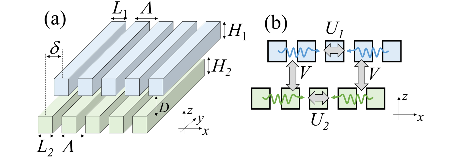
Figure 1: (a) A photonic crystal consists of two gratings corrugated along the $x$-axis with the same period $\Lambda$. The sizes of the rod of the two gratings are slightly different from each other and can be tuned to induce different topological phases. The lateral shift plays the role of a synthetic dimension beside the genuine Bloch momentum along the $x$-axis. (b) Sketch of the plane wave guided modes and their intra- and inter-layer coupling mechanisms at the edge of the Brillouin zone.

We consider in this work the extension of the momentum space by an additional parameter, regarded as a synthetic momentum. This leads to the band structure over a hybrid Brillouin zone consisting of one genuine and another synthetic momentum. Topological aspects of the band theory in this hybrid momentum space are unconventional, exhibiting non-trivial geometry and topology even in the presence of both time reversal and spatial inversion symmetry. This is in a sharp contrast to that of traditional electronic band structures, in which non-zero Berry curvature requires symmetry breaking [39]. The system is realised by a 1D system of bilayer photonic grating, with the translational displacement between the two layers naturally taking the role of the synthetic momentum. Remarkably, the resulted band structure not only realises the interesting dynamics of merging and splitting of twin Dirac points, but also gap opening as the system parameters vary [40, 41, 42, 43, 44]. We propose a simple topological argument to analyse the associated topological phase transitions. The non-trivial topological phases are clearly demonstrated by the presence of robust optical edge modes at their junctions, much in similarity to the quantum Hall effect in condensed matter systems. Our work therefore opens a new view point on topological aspects of band theory with promising new physics unfamiliar to traditional theory of photonic crystals.

Synthetic momentum— To this end, we consider an explicit physical setup of two grating layers separated by a distance $D$ as depicted in Fig. 1. They share the same period $\Lambda$, but are slightly shifted by a relative displacement $\delta\in\left[-\frac{\Lambda}{2},\frac{\Lambda}{2}\right]$. The sizes of the rods of the gratings are slightly different ($H_{1}\approx H_{2}$, $L_{1}\approx L_{2}$), which will be tuned to induce different topological phases. Here the materials are of high refractive index and all geometrical parameters are of subwavelength scale, leading to strong intra-layer diffractive mechanisms and inter-layer evanescence.[45, 46]

Ignoring the homogeneous dimension $y$, the system is effectively a 1D photonic crystal along the $x$-axis. For each momentum $q_{x}$ in the first Brillouin zone of the corresponding reciprocal lattice, the permissible light modes are indicated by an energy $E$ from a typically discrete set of values from photonic band structure. Here, we use ‘momentum’ and ‘wavevector’ interchangeably, and likewise for ‘energy’ and ‘frequency’.

In the vicinity of the edge of the Brillouin zone (i.e. $X$ point), the photonic modes can be described by a four-component spinor $\Psi(x)$ evolving under an effective Hamiltonian in the momentum space $q_{x}$, given by  [45, 46]

$$H(q_{x},\delta)=\omega_{0}+\left(\begin{matrix}vq_{x}&U+\Delta&Ve^{\frac{-i\pi\delta}{\Lambda}}&0\\ U+\Delta&-vq_{x}&0&Ve^{\frac{i\pi\delta}{\Lambda}}\\ Ve^{\frac{i\pi\delta}{\Lambda}}&0&vq_{x}&U-\Delta\\ 0&Ve^{\frac{-i\pi\delta}{\Lambda}}&U-\Delta&-vq_{x}\end{matrix}\right).$$ (1)

The first(second) two components of the spinor $\Psi(x)$ correspond to the enveloping amplitudes of the right-travelling and left-travelling light modes at the $X$ point for the upper(lower) grating in the absence of the modulation of the refraction index. The corrugation induces a diffractive coupling between these opposite-travelling modes with coupling strength $U\pm\Delta$ (see Fig. 1b). The difference in the coupling strength $\Delta$ is induced by a thickness or the size difference between the two gratings  [47]. Importantly, the light modes travelling in the same direction but from different gratings are coupled via the evanescent mechanism by a complex strength with the phase-shift induced by the displacement $\delta$ between the two gratings, $Ve^{-\frac{i\pi\delta}{\Lambda}}$. The coupling amplitude $V$ can be tuned via the distance $D$ separating the two gratings.

For a given displacement $\delta$, the Hamiltonian (1) is 1D. Although the system can have non-trivial topological phases, the associated Berry curvature vanishes [48]. To enable the investigation of the topological phases of the system via the Berry curvature, the key idea is now to regard the displacement as a synthetic momentum, more precisely, $q_{y}=\delta/\Lambda$. We therefore consider the band structure over a hybrid momentum space $(q_{x},q_{y})$. We are to show that the system surprisingly allows for different topological phases in this hybrid momentum space even in the presence of time reversal and inversion symmetry.

Symmetry and Berry curvature— The crucial point underlying the non-trivial topology of the system is the unusual behaviour of the synthetic momentum $q_{y}$ under time reversal transformation. Unlike a genuine momentum, which reverses its direction under time reversal, the synthetic momentum $q_{y}$ remains invariant as it is defined by the spatial displacement of two structures, $q_{y}=\delta/\Lambda$. As a result, the time reversal symmetry of the Hamiltonian (1) is described by $H(q_{x},q_{y})=T^{\dagger}H(-q_{x},q_{y})T$, where $T=(\mathbb{I}\otimes\sigma_{x})K$. Here $K$ is the complex conjugate operator. Accordingly the eigen energy $\omega(q_{x},q_{y})$ and the eigenstates $u(q_{x},q_{y})$ are related by $\omega(q_{x},q_{y})=\omega(-q_{x},q_{y})$ and $u(q_{x},q_{y})=(\mathbb{I}\otimes\sigma_{x})u^{\ast}(-q_{x},q_{y})$. One then can verify directly that the components of the Berry vector potential (Berry connection), defined by $\vec{A}(q_{x},q_{y})=i\bra{u({q_{x},q_{y}})}\left.\nabla_{q_{x},q_{y}}u({q_{x},q_{y}})\right\rangle$, obey the symmetry $A^{x}(-q_{x},q_{y})=A^{x}(-q_{x},q_{y})$ and $A^{y}(-q_{x},q_{y})=-A^{y}(-q_{x},q_{y})$. As a result, the Berry curvature $b(q_{x},q_{y})=\operatorname{rot}\vec{A}$ obeys $b(q_{x},q_{y})=b(-q_{x},q_{y})$.

Remarkably, the setup as sketched in Fig. 1 is not invariant under spatial inversion – here indicating the $x$-reflection – while the Hamiltonian (1) does express the inversion symmetry. This is because the Hamiltonian (1) in fact encapsulates all different physical realisations of the system corresponding to different $\delta$. Formally, the inversion symmetry of the Hamiltonian (1) is an authentic 2D inversion symmetry where both $q_{x}$ and $q_{y}$ acquire a minus sign, and therefore $b(q_{x},q_{y})=b(-q_{x},-q_{y})$.

Together time reversal and spatial inversion symmetry imply that $b(q_{x},q_{y})=b(-q_{x},q_{y})=b(q_{x},-q_{y})=b(-q_{x},-q_{y})$. One sees then, unlike traditional electronic bands, the Berry curvature is not constrained to vanish despite the presence of time reversal and spatial inversion symmetry. As long as the band is separated by a finite gap, the total Berry flux can be computed by integrating the Berry curvature and topological phases can be identified . Explicit computation shows that the Berry curvature is indeed non-zero. Remarkably, the system also expresses interesting dynamics of merging Dirac points and gap opening in the band structure, and therewith the associated topological phase transitions.

Band structure, Dirac point merging, gap opening, topology and edge states— Fig. 2a-i presents the band structure of the system calculated from Hamiltonian (1). The four energy bands are separated by three gaps, each can be opened at certain values of the controlling parameters $\Delta$ and $\Gamma=U-\sqrt{V^{2}+\Delta^{2}}$. The upper and lower gaps are opened at separated (upper and lower) Dirac points at the high symmetry point $(q_{x}=0,q_{y}=1/2)$ as long as $\Delta\neq 0$. The Berry curvature around the upper and lower Dirac points follow standard rules of condensed matter physics: across the transition from $\Delta<0$ to $\Delta>0$ along the columns of Fig. 2a-i, the contribution $\pm\pi$ to the total Berry flux of each Dirac point changes signs; the Chern numbers therefore change by one unit.

We concentrate here on the evolution of the middle gap along the rows of Fig. 2a-i and analyse their contribution to the total Berry flux. Consider the case $\Delta=0$, i.e., Fig. 2d-e-f. Starting from the left panel, $\Gamma<0$, the two middle bands cross at a pair of twin Dirac points located at $(q_{x}=\pm k_{D},q_{y}=0)$, with $k_{D}=\frac{\sqrt{V^{2}-U^{2}}}{v}$ (Fig. 2d). Increasing $\Gamma$ causes the twin Dirac points to approach each other and eventually merge into a single semi-Dirac point (quadratic dispersion in $q_{x}$ and linear dispersion in $q_{y}$) at $\Gamma=0$ (Fig. 2e). As long as $\Gamma>0$, a gap is opened (Fig. 2f). This merging of the twin Dirac points follows the generic mechanism proposed in Ref. [40, 41]. The effective Hamiltonian at $\Delta=0$ near the merging point can be expressed in terms of a generic two-level Hamiltonian [47, Secion S3]

$$H=h_{x}\sigma_{x}+h_{y}\sigma_{y}+h_{z}\sigma_{z}$$ (2)

with $h_{x}=q_{x}^{2}v^{2}/(2U)+\Gamma$, $h_{y}=q_{y}V\pi$ and $h_{z}=0$. Here $\sigma_{x}=\begin{pmatrix}0&1\\ 1&0\end{pmatrix}$ and $\sigma_{y}=\begin{pmatrix}0&i\\ -i&0\end{pmatrix}$ are the Pauli matrices. To understand the change of the total Berry flux, we consider the surface determined by $h_{x}(q_{x},q_{y})$ and $h_{y}(q_{x},q_{y})$ in the space of three components of $(h_{x},h_{y},h_{z})$. It is interesting to see that $h_{x}$ depends on $q_{x}$ quadratically, therefore as $q_{x}$ and $q_{y}$ vary, $h_{x}$ and $h_{y}$ form a double half-plane folded along $h_{x}=\Gamma$ as shown in Fig. 2d’-e’-f’. For $\Gamma<0$, this folded half-plane contains the origin (Fig. 2d’), causing the gap closing at two points $q_{x}\propto\pm\sqrt{\Gamma}$, while for $\Gamma>0$ it does not and a gap presents (Fig. 2f’). Remarkably, as long as $\Delta\neq 0$, a gap opens at the two Dirac points in Fig. 2d, resulting in band structures shown in Fig. 2a and g. That means that the double half-plane in Fig.  2d’-e’-f’ are slightly unfolded as shown in Fig. 2a’-b’-c’ or Fig. 2g’-h’-i’. Now recalling that the local contribution to the total Berry flux of the band is exactly the flux through this surface by a monopole placed at the origin [48], one can easily read off all the expected contributions to the total Berry flux indicated in Fig. 2. In particular, the transitions along the upper and lower row, Fig. 2a-b-c and Fig. 2g-h-i, correspond to the crossing of the monopole through the folded edge, Fig. 2a’-b’-c’ and Fig. 2g’-h’-i’, therefore the contributed Berry flux changes one unit of $2\pi$ (Chern number changes by $\pm 1$). Moreover, the transition along the first column, Fig. 2a-d-g, causes the plane to fold back into the degenerate form (Fig. 2d) before unfolding again; the two sides of the plane exchange inside out, causing a change of Berry flux to change by $4\pi$ (the Chern number changes by $\pm 2$). For an analysis based on detailed effective Hamiltonians near the transitions, see [47].

The topological phases of the system are associated to the formation of edge states at the junction of two different phases, following chiral dispersion relations connecting the lower band on one side to the upper band of the other side [47]. In particular, a junction corresponding to the transition Fig. 2a-b-c or Fig. 2g-h-i accommodates one edge state according the edge-boundary correspondence rule, as the Chern number by $\pm 1$ across the junction. Otherwise, across a junction corresponding to the transition Fig. 2a-d-g, the Chern number changes by $\pm 2$, resulting in two edge states. All these predictions are confirmed by a highly accurate Finite-Difference Time-Domain (FDTD) simulation of the realisation of a system below.

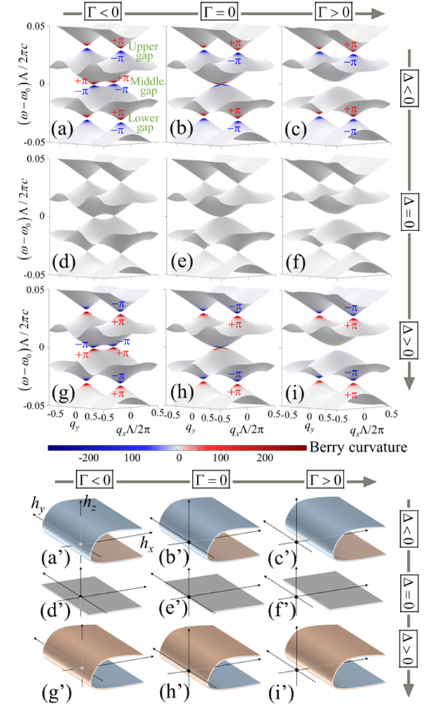
Figure 2: Upper panel: Theoretical band structures and the associated local Berry flux contribution (in unit of $2\pi$) corresponding to (a) $\Delta=-0.05U,\,\Gamma=-0.1U$, (b) $\Delta=-0.05U,\,\Gamma=0$, (c) $\Delta=-0.05U,\,\Gamma=0.1U$,(d) $\Delta=0,\,\Gamma=-0.1U$, (e) $\Delta=0,\,\Gamma=0$, (f) $\Delta=0,\,\Gamma=0.1U$, (g) $\Delta=0.05U,\,\Gamma=0.1U$, (h) $\Delta=0.05U,\,\Gamma=0$, (i) $\Delta=0.05U,\,\Gamma=-0.1U$. Lower panel: the surface mapped by the vector $\vec{h}=(h_{x},h_{y},h_{z})$ as functions of $(q_{x},q_{y})$ for each case of (a-i).

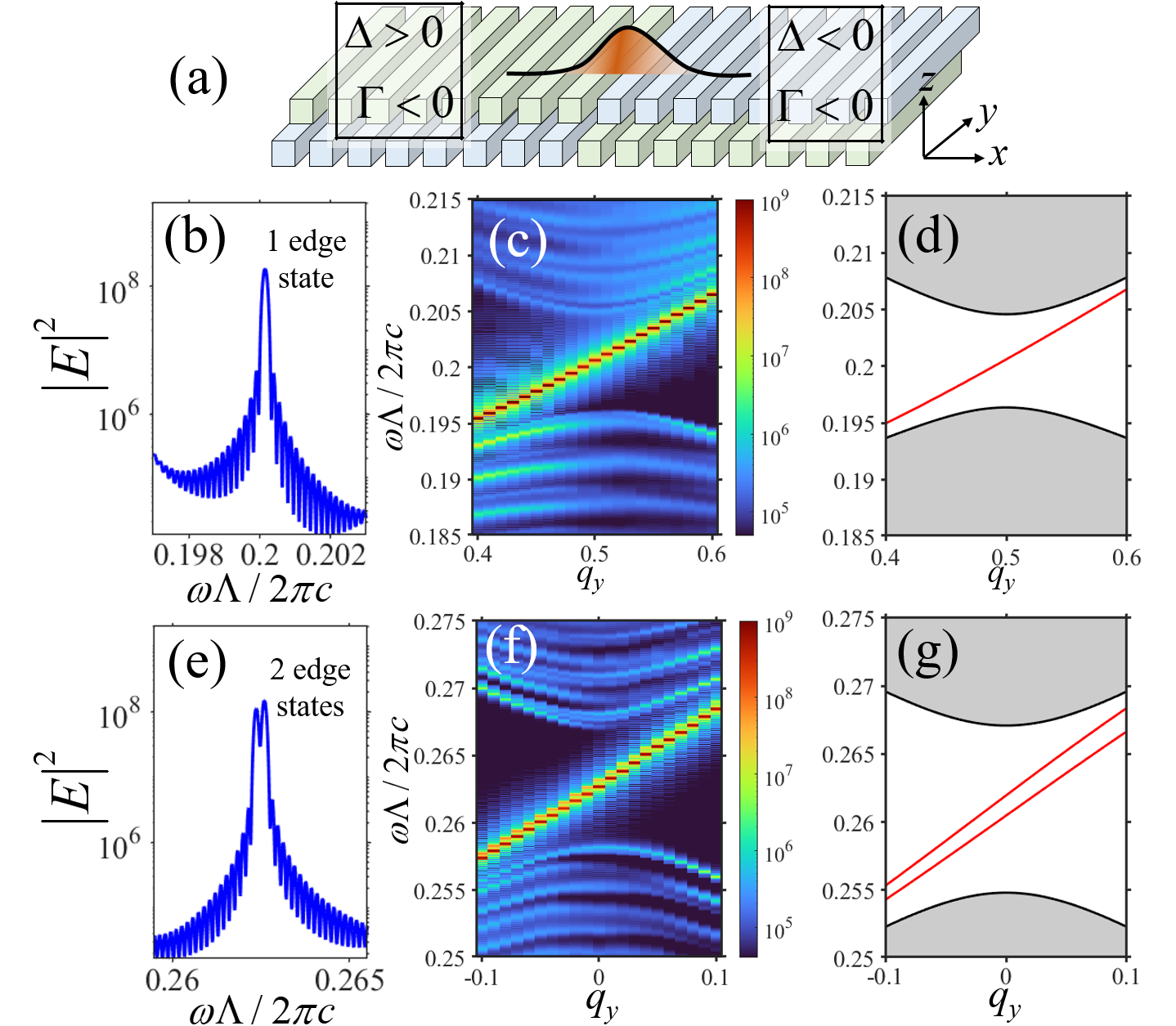
Figure 3: (a) Sketch of the setup for an “heterostructure” consisting of two different topological phases. The left and the right structure are identically manufactured, but the upper and lower grating swapped.The parameters of the left structure are $H_{1}=H_{2}=0.37\Lambda$, $L_{1}=0.75\Lambda$ and $L_{2}=0.85\Lambda$. There is no distance separating the upper and lower gratings. The parameters of the right structure are the same, except for the swapping between the values of $L_{1}$ and $L_{2}$. (b,e) Simulated spectra in the vicinity of (b) the lower gap at $\mathbf{q}_{y}=0.5$ and (e) the middle gap at $q_{y}=0$. (c,f) Simulated spectra in the vicinity of (c) the lower gap when scanning $q_{y}$ from 0.4 to 0.6, (f) the upper gap when scanning $q_{y}$ from -0.1 to 0.1. (d,g) Theoretical prediction of (c,f) using the effective theory (1).

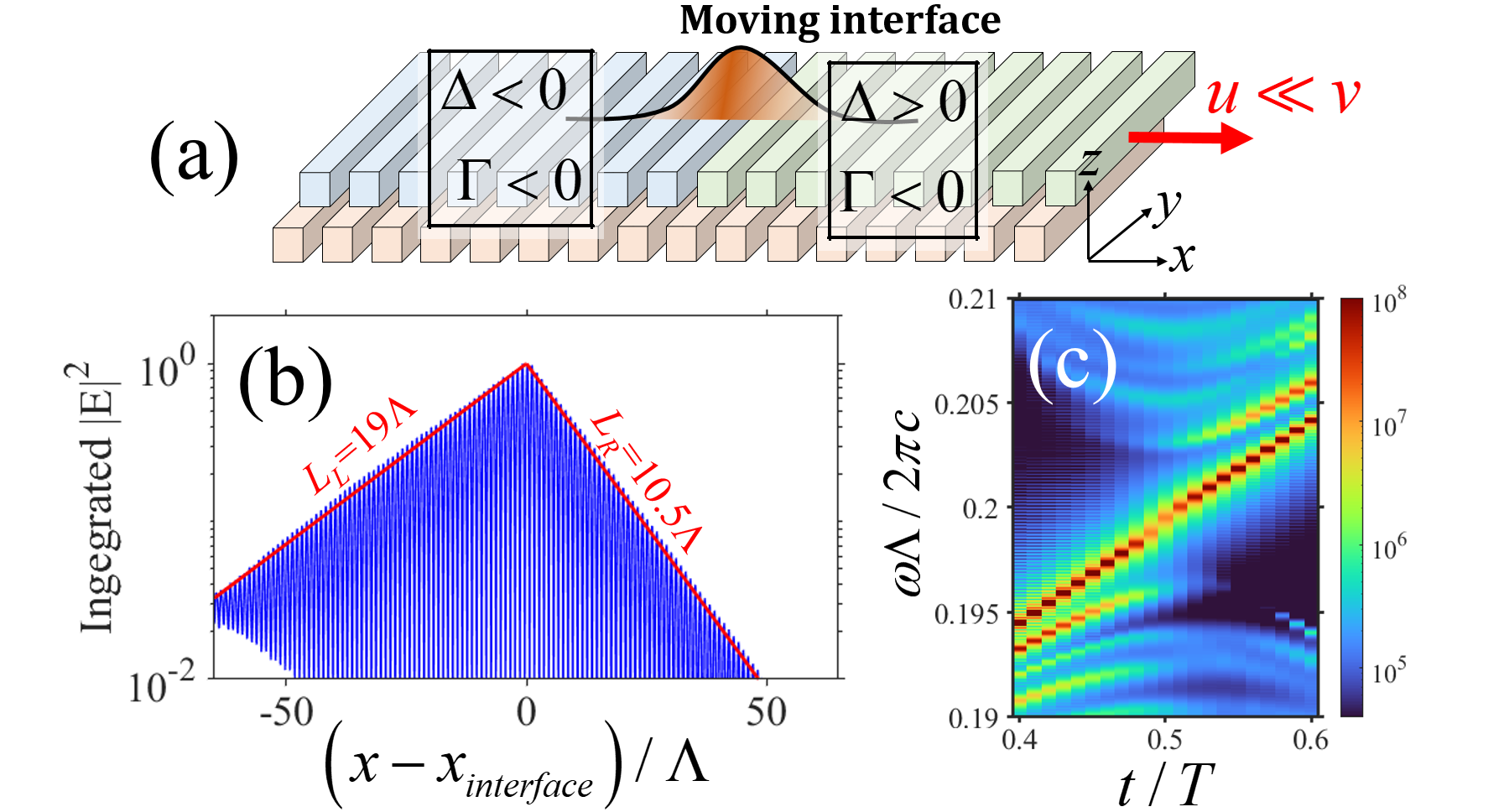
Figure 4: (a) Sketch of the setup for a moving interface separating two different topological phases. The upper heterogeneous grating slides slowly, while the lower homogeneous grating is fixed. The parameters for the left(right) part of the upper grating are $L_{1(2)}=0.85(0.75)\Lambda$ and $H_{1(2)}=0.37(0.4)\Lambda$. The parameters for the lower grating are $L_{3}=0.8\Lambda$ and $H_{3}=0.37\Lambda$. There is no distance separating the upper and lower gratings. (b) Simulation results for the localization of the edge state within the lower gap at $\delta=0.5$. (c) Simulated spectra in the vicinity of the lower gap, showing the spectral flow of the edge state in time.

Edge states and adiabatic pumping— Fig. 3a sketches a heterogeneous junction, in which the left and right bulk have the same design, but the upper and the lower grating are swapped. FDTD simulations on a realistic design with gratings made of silicon (refractive index $n=3.4$) and period $\Lambda=300$$\mathrm{nm}$ for an operation in the telecom wavelength range ($\lambda\approx 1.5$$\mathrm{nm}$) are performed [47]. Here for the simplicity, we only focus on the lower and the middle gap and discuss the upper gap in the Supplement [47]. The reason is that the system turns out also support states at different momenta in the energy range of the upper gap, slightly smearing out the observation of the edge state [47]. The simulations confirm the localization at the heterostructure interface of a single edge state within the lower gap and double edge states within the middle gap, exponentially decaying into the bulks [47]. This corresponds respectively to the single lower Dirac point and the twin middle Dirac points in the bulks at $\Delta=0$ (Fig. 2a). The FDTD simulations also confirm the protection of the chirality against perturbation [47]. The unidirectional propagation of these edge states connecting the bulk-bands are observed (Fig. 3c,f) in an excellent agreement with the effective theory (Fig. 3d,g). One may notice that the degeneracy lifting of the two edge states in the middle gap calculated by the effective theory (Fig. 3g) is more pronounced than the one provided by simulations (Fig. 3f). In addition, we observe that while these states are topologically protected, their energy splitting is rather sensitive to perturbations on the interface [47].

Unlike the Bloch momenta, synthetic momentum can be easily dynamically driven. One may fabricate a mobile heterogeneous upper grating on top of a homogeneous lower one and move it slowly from left to right (see Fig. 4a). The left side of the moving junction has $\Delta<0$, while the right side one has $\Delta>0$. Particular cares in the design are made to ensure overlap between lower gaps from each side.Each time the upper grating move a distance of $\Lambda$ corresponds to one evolution $q_{y}$ across the synthetic Brillouin zone. Figure 4b depicts a snapshot of localization of lower-gap edge state at particular instant of the moving interface. The simulation results demonstrate clearly the evolution of the edge state dispersion flow connecting the two bulk bands (Fig. 4c), which is nicely reproduced by the effective theory [47]. After each period, a light mode is pumped from the left to the right along the edge state dispersion. Experimentally the edge states are excited by implementing active (i.e., gain) materials at the interface and perform non-resonant optical pumping to make lasing action at the edge state. In this way, the edge state is selectively and continuously pumped throughout its evolution in time. Such unique scheme, only possible in photonic platform, have been experimentally used to demonstrate the lasing action at topological edge states in 1D chain [50, 51, 52, 53].

Conclusion— We have demonstrated that unconventional topological phenomena in a simple optical system in hybrid momentum space deviate from the normal framework of topological insulators. Experimental realisation can be carried out within current silicon technology with standard nanofabrication processes. Further investigation of optical or condensed matter physics systems in hybrid momentum space is a very promising direction for future research. Particularly interesting is the possibility of having unconventional high dimensional topological band theory by introducing sufficient synthetic dimensions in optical setups, for instant one may think of increase the number of layers or using bidimensional photonic crystal instead of gratings. Finally, the possibility to implement gain/losses in the photonic platform paves the way to explore new features of non-hermitian topology with synthetic momentum.

The authors thank Pierre Delplace and David Carpentier for fruitful discussions. This work was partly funded by the French National Research Agency (ANR) under the project POPEYE (ANR-17-CE24-0020) and the IDEXLYON from Université de Lyon, Scientific Breakthrough project TORE within the Programme Investissements d’Avenir (ANR-19-IDEX-0005). DXN was supported by Brown Theoretical Physics Center. HCN was supported by the Deutsche Forschungsgemeinschaft (DFG, German Research Foundation, project numbers 447948357 and 440958198), the Sino-German Center for Research Promotion (Project M-0294), and the ERC (Consolidator Grant 683107/TempoQ).

— Supplementary Material —
Topological Properties of Photonic Bands with Synthetic Momentum
H. Chau Nguyen, Dung Xuan Nguyen, Xavier Letartre, Piere Viktorovitch, and Hai-Son Nguyen

Appendix S1 The effective Hamiltonian for light for double layer crystal

The system studied in this manuscript is sketched in Fig. 1(a). It consists of two uni-dimensional (1D) photonic grating sharing the same subwavelength period $\Lambda$ separated by a distance $D$. The sizes of the slabs in the two gratings are slightly different from each other ($H_{1}\approx H_{2}$, $L_{1}\approx L_{2}$). The geometrical parameters of the systems are of subwavelength. We consider a given transverse polarization (in the numerical simulation, the considered polarization is Transverse Electric (TE), and the wave function is reduced to a scalar wave $E_{y}$). Several aspects of such a system has been analysed in Ref. [45, 46].

The effective theory for the system can be carried out in much similarity to the near-free-electron model in condensed matter physics [54]. In this framework, the modulation of the refraction index is considered as a perturbation on top of a homogeneous media. Consider the system without the modulation of the refraction index, then the light modes are simply plane wave (with possibly nonlinear dispersion relation.) The perturbation caused by the modulation of the refraction index causes Bragg diffraction of the light by its regular structure of period $\Lambda$. The diffraction is particularly important at the edge of the Brillouin zone $\pi/\Lambda$ (the $X$ point), where the perturbation couples nearly generate modes of the same energy. The operating spectral range is chosen to be in the vicinity of the frequency $\omega_{0}$ corresponding to this Brillouin zone edge. Precisely at the $X$ point, the unperturbed guided modes consist of forward ($\ket{\phi_{1,+}},\ket{\phi_{2,+}}$) and backward ($\ket{\phi_{1,-}},\ket{\phi_{2,-}}$) propagating plane waves [see Fig. 1(b)]. Slightly away from the $X$ point, indicated by the shifted-momentum $k$ around $\pi/\Lambda$, the dispersion relationship of the unperturbed guided modes is given by linear characteristics,

$$\omega_{\pm}(k)=\omega_{0}\pm vk.$$ (S1.1)

Here the sign “+” is for forward and “-” is for backward modes, with $v$ being the group velocity at the edge of the Brillouin zone $\pi/\Lambda$. As discussed in the main text and in Ref. [45, 46], there are two coupling mechanisms induced by the modulation of the refraction index [see Fig. 1(b)] :

• Intra-layer coupling: Counter-propagating guided modes of the same layer are coupled via diffraction process induced by the periodic corrugation. The corresponding coupling strengths are $U_{1}$ and $U_{2}$ for upper and lower layer respectively (these coupling strength can be evaluated from the first Fourier component of the dielectric function of the slabs). In the following, we choose to work with $U$ and $\Delta$ which are defined by $U=\frac{U_{1}+U_{2}}{2}$ and $\Delta=\frac{U_{1}-U_{2}}{2}$.

• Inter-layer coupling: Co-propagating guided modes from separated layers are coupled via evanescent effect (i.e., near-field coupling). Such coupling is characterized by the a complex coupling factor $Ve^{i\varphi}$. Here the coupling phase $\varphi$ is given by the relative displacement $\delta$ between the two layer,

  $$\varphi=\pi\frac{\delta}{\Lambda}$$ (S1.2)

Together, the Hamiltonian is given by [45, 46]

$$H(q_{x},\delta)=\omega_{0}+\left(\begin{matrix}vq_{x}&U+\Delta&Ve^{\frac{-i\pi\delta}{\Lambda}}&0\\ U+\Delta&-vq_{x}&0&Ve^{\frac{i\pi\delta}{\Lambda}}\\ Ve^{\frac{i\pi\delta}{\Lambda}}&0&vq_{x}&U-\Delta\\ 0&Ve^{\frac{-i\pi\delta}{\Lambda}}&U-\Delta&-vq_{x}\end{matrix}\right).$$ (S1.3)

We regard the phase $q_{y}=\delta/\Lambda$ as a synthetic momentum with the first Brillouin zone defined by $q_{y}\in[-1/2,+1/2]$. Such a Brillouin zone size is unusual for a phase parameter $e^{i\varphi}$, is due to the periodicity $\Lambda$ of the displacement $\delta$. The hybrid 2D momentum space, the synthetic momentum space (SMS), mapped by $(q_{x},q_{y})$ is therefore continuous along $q_{x}$-axis and of period $1$ along $q_{y}$-axis.

Appendix S2 Symmetry and Berry phase

To investigate the symmetry of the Hamiltonian $H$ given in Eq. (1), we take out the off set $\omega_{0}$:

$$H(q_{x},q_{y})=\left(\begin{matrix}vq_{x}&U+\Delta&Ve^{-i\pi q_{y}}&0\\ U+\Delta&-vq_{x}&0&Ve^{+i\pi q_{y}}\\ Ve^{+i\pi q_{y}}&0&vq_{x}&U-\Delta\\ 0&Ve^{-i\pi q_{y}}&U-\Delta&-vq_{x}\end{matrix}\right),$$ (S2.4)

which can also be writen as

$$H(q_{x},q_{y})=vq_{x}\mathbb{I}\otimes\sigma_{z}+U\mathbb{I}\otimes\sigma_{x}+\Delta\sigma_{z}\otimes\sigma_{x}+V[\sigma_{+}\otimes e^{-i\pi q_{y}\sigma_{z}}+\sigma_{-}\otimes e^{+i\pi q_{y}\sigma_{z}}].$$ (S2.5)

Here $\otimes$ is the Kronecker product, $\sigma_{i}$ is Pauli matrice defined by:

$$\sigma_{x}=\left(\begin{matrix}0&1\\ 1&0\end{matrix}\right),\quad\sigma_{y}=\left(\begin{matrix}0&-i\\ i&0\end{matrix}\right),\quad\sigma_{z}=\left(\begin{matrix}1&0\\ 0&-1\end{matrix}\right),\quad\sigma_{\pm}=(\sigma_{x}\pm i\sigma_{y})/2.$$ (S2.6)

We now consider the symmetry of the Hamiltonian in the parameter space of $(q_{x},q_{y})$, thereby derive the symmetry of the Berry curvature. Although $q_{y}$ is regarded as a synthetic momentum, it is in fact of spatial nature since it is defined from the relative displacement $\delta/\Lambda$. Therefore, unlike a genuine momentum, which changes its sign under time reversal symmetry, $q_{y}$ remains invariant under time reversal symmetry. This leads to the possibility of having non-zero local and total Berry curvature even in the presence of both time reversal symmetry and spatial inversion symmetry.

S2.1 Symmetries of fish-bone Hamiltonian

Let us start with listing the symmetry of the Hamiltonian:

• Time reversal symmetry. As discussed above, the time reversal action would only flip the sign of the genuine momentum $q_{x}$, thus its action in the synthetic momentum space (SMS) corresponds to $(q_{x},q_{y})\xrightarrow{T}(-q_{x},q_{y})$. Let $K$ be the complex conjugation $KiK^{-1}=-i$, one can check that

  $$H(q_{x},q_{y})=(\mathbb{I}\otimes\sigma_{x})KH(-q_{x},q_{y})K(\mathbb{I}\otimes\sigma_{x}),$$ (S2.7)

  thus the time reversal operator is given by:

  $$T=(\mathbb{I}\otimes\sigma_{x})K,$$ (S2.8)

  which is expected, since under time reversal transformation, the forward ‘$+$’ modes and the backward ‘$-$’ modes are exchanged. This exchange is implemented by the operator $\mathbb{I}\otimes\sigma_{x}$.

• Spatial inversion. Here spatial inversion refers to the $x$-reflection. The mirror reflection along $x$-axis (i.e., horizontal flip) would change sign of both the momentum $q_{x}$ and the relative displacement $\delta$. Its action in the SMS corresponds to $(q_{x},q_{y})\xrightarrow{M_{x}}(-q_{x},-q_{y})$. One can check that

  $$H(q_{x},q_{y})=(\mathbb{I}\otimes\sigma_{x})H(-q_{x},-q_{y})(\mathbb{I}\otimes\sigma_{x}),$$ (S2.9)

  thus the $x$-reflection operator is given by

  $$M_{x}=\mathbb{I}\otimes\sigma_{x}.$$ (S2.10)

  Again $\mathbb{I}\otimes\sigma_{x}$ implements the switching of ‘$+$’ modes and ‘$-$’ modes as the consequence of the $x$-reflection.

• $z$-reflection. If the two layers are identical (i.e., $\Delta=0$), the system also expresses the mirror reflection along $z$-axis (i.e. vertical flip). Its action keeps the momentum $q_{x}$ unchanged but switch sign of and the relative displacement $\delta$, corresponding to $(q_{x},q_{y})\xrightarrow{M_{z}}(q_{x},-q_{y})$. One can check that at $\Delta=0$,

  $$H(q_{x},q_{y})=(\sigma_{x}\otimes\mathbb{I})H(q_{x},-q_{y})(\sigma_{x}\otimes\mathbb{I}),$$ (S2.11)

  thus the z-reflection operator is represented by:

  $$M_{z}=\sigma_{x}\otimes\mathbb{I}.$$ (S2.12)

  The operator $\sigma_{x}\otimes\mathbb{I}$ plays the role of switching layers which is the consequence of $z$-reflection.

• Particle-hole symmetry. Interestingly, the Hamiltonian (S2.4) also allows for the particle hole symmetry,

  $$-H(q_{x},q_{y})=(\sigma_{z}\otimes\sigma_{y})KH(q_{x},q_{y})K(\sigma_{z}\otimes\sigma_{y}),$$ (S2.13)

  The particle hole symmetry operator is given by

  $$PH=(\sigma_{z}\otimes\sigma_{y})K.$$ (S2.14)

  As the consequence of particle-hole symmetry, if the eigenstate $|u_{q_{x},q_{y}}\rangle$ has energy $\omega_{q_{x},q_{y}}$, then the state $\sigma_{z}\otimes\sigma_{y}|u^{\ast}_{q_{x},q_{y}}\rangle$ is an eigenstate with energy $-\omega_{q_{x},q_{y}}$.

S2.2 Symmetry of the Berry curvature

We will derive the symmetry of the Berry curvature inherited from the symmetry of the Hamiltonian. The two symmetry operations that are here important are the time reversal and the spatial inversion. The Berry connection is defined as [48]

$$\vec{A}(q_{x},q_{y})=i\bra{u_{q_{x},q_{y}}}|\vec{\nabla}u_{q_{x},q_{y}}\rangle.$$ (S2.15)

with $\vec{\nabla}=(\partial_{q_{x}},\partial_{q_{y}})$. The Berry curvature in the hybrid momentum space $(q_{x},q_{y})$ is given by [48]

$$b(q_{x},q_{y})=\partial_{q_{y}}A^{x}-\partial_{q_{x}}A^{y}.$$ (S2.16)

Time reversal symmetry. The time reversal symmetry implies that if $\ket{u_{q_{x},q_{y}}}$ is an eigenvector of $H(q_{x},q_{y})$ of energy $\omega_{q_{x},q_{y}}$, then $\ket{u_{-q_{x},q_{y}}}=T\ket{u_{q_{x},q_{y}}}$ is an eigenvector if $H(-q_{x},q_{y})$ of energy $\omega_{-q_{x},q_{y}}=\omega_{q_{x},q_{y}}$. Therefore, we have

$$A^{x}(-q_{x},q_{y}) =-i\bra{u_{-q_{x},q_{y}}}\left.\partial_{q_{x}}u_{-q_{x},q_{y}}\right\rangle$$

$$=-i\bra{u_{q_{x},q_{y}}^{\ast}}\left.\partial_{q_{x}}u_{q_{x},q_{y}}^{\ast}\right\rangle$$

$$=i\bra{u_{q_{x},q_{y}}}\left.\partial_{q_{x}}u_{q_{x},q_{y}}\right\rangle$$

$$=A^{x}(q_{x},q_{y}).$$ (S2.17)

where we have used $M_{x}^{\dagger}M_{x}=\mathbb{I}\otimes\mathbb{I}$ and the reality of the vector potential. Likewise

$$A^{y}(-q_{x},q_{y}) =i\bra{u_{-q_{x},q_{y}}}\left.\partial_{q_{y}}u_{-q_{x},q_{y}}\right\rangle$$

$$=i\bra{u_{q_{x},q_{y}}^{\ast}}\left.\partial_{q_{y}}u_{q_{x},q_{y}}^{\ast}\right\rangle$$

$$=-i\bra{u_{q_{x},q_{y}}}\left.\partial_{q_{y}}u_{q_{x},q_{y}}\right\rangle$$

$$=-A^{y}(q_{x},q_{y}).$$ (S2.18)

With the definition of the Berry curvature (S2.16), we obtain the relation

$$b(-q_{x},q_{y}) =\partial_{q_{y}}A^{x}(-q_{x},q_{y})+\partial_{q_{x}}A^{y}(-q_{x},q_{y})$$

$$=\partial_{q_{y}}A^{x}(q_{x},q_{y})-\partial_{q_{x}}A^{y}(q_{x},q_{y})$$

$$=b(q_{x},q_{y}),$$ (S2.19)

as the consequence of the time reversal symmetry.

Spartial inversion symmetry. The spatial inversion symmetry implies that if $\ket{u_{q_{x},q_{y}}}$ is an eigenvector of $H(q_{x},q_{y})$ of energy $\omega_{q_{x},q_{y}}$, then $\ket{u_{-q_{x},-q_{y}}}=M_{x}\ket{u_{q_{x},q_{y}}}$ is an eigenvector if $H(-q_{x},-q_{y})$ of energy $\omega_{-q_{x},-q_{y}}=\omega_{q_{x},q_{y}}$. Similarly to the analysis of the time reversal symmetry, we now have:

$$A^{x}(-q_{x},-q_{y}) =-i\bra{u_{-q_{x},-q_{y}}}\left.\partial_{q_{x}}u_{-q_{x},-q_{y}}\right\rangle$$

$$=-i\bra{u_{q_{x},q_{y}}}\left.\partial_{q_{x}}u_{q_{x},q_{y}}\right\rangle$$

$$=-A^{x}(q_{x},q_{y}).$$ (S2.20)

We also have

$$A^{y}(q_{x},q_{y}) =-i\bra{u_{-q_{x},-q_{y}}}\left.\partial_{q_{y}}u_{-q_{x},-q_{y}}\right\rangle$$

$$=-i\bra{u_{q_{x},q_{y}}}\left.\partial_{q_{y}}u_{q_{x},q_{y}}\right\rangle$$

$$=-A^{y}(q_{x},q_{y}).$$ (S2.21)

Combining with the definition of Berry curvature (S2.16), we obtain the relation

$$b(-q_{x},-q_{y}) =-\partial_{q_{y}}A^{x}(-q_{x},-q_{y})+\partial_{q_{x}}A^{y}(-q_{x},-q_{y})$$

$$=\partial_{q_{y}}A^{x}(q_{x},q_{y})-\partial_{q_{x}}A^{y}(q_{x},q_{y})$$

$$=b(q_{x},q_{y}).$$ (S2.22)

Combining both time reversal symmetry and spatial inversion symmetry together, we arrive at

$$b(q_{x},q_{y})=b(-q_{x},q_{y})=b(q_{x},-q_{y})=b(-q_{x},-q_{y}).$$ (S2.23)

Unlike the usual electronic bands, the Berry curvature and therefore its integral over the hybrid Brillouin zone does not vanish even with the appearance of both time reversal and spatial reflection.

Lastly it is easy to see that the consequence of the particle-hole symmetry implies that the particle-hole conjugated bands have opposite Berry curvature at the same momentum $(q_{x},q_{y})$.

Appendix S3 Dirac cones in the band structure at $\Delta=0$

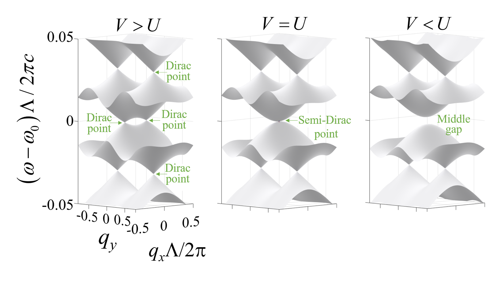
Figure S1: Band structure of the“fish-bone” lattice when the gratings are identical (i.e. $\Delta=0$). Three distinctive scenario are presented, corresponding to $V<U$(a), $V=U$(b) , $V>U$(c).

In this section, the case of two identical gratings (i.e. $\Delta=0$) will be investigated. We will see that, in this configuration, the effective Hamiltonians near the band-crossing points are Dirac Hamiltonians in the synthetic momentum space. By tuning the parameters of the fish-bone Hamiltonian (S1.3), we also obtain the merging and splitting Dirac winding number phenomena which were investigated in semimetals previously [41]. Let us remind the definition of winding number and the Berry flux of a 2D Dirac cone.

Winding number and Berry flux of a 2D Dirac cone

We consider the effective 2D Dirac hamiltonian

$$H_{D}=v_{x}k_{x}\sigma_{x}+v_{y}k_{x}\sigma_{y}$$ (S3.24)

with $v_{x}$ and $v_{y}$ are velocities in the $\hat{x}$ and $\hat{y}$ directions. $k_{x}$ and $k_{y}$ are the shift of momentum from the origin of the Dirac cone. One can obtain the eigenstate

$$\psi_{\lambda,\vec{k}}=\frac{1}{\sqrt{2}}\left(\begin{matrix}1\\ \lambda e^{i\phi_{\vec{k}}}\end{matrix}\right),$$ (S3.25)

with $\lambda=\pm 1$ is the band index corresponds to the eigen-energies

$$\epsilon_{\lambda}(\vec{k})=\lambda\sqrt{v_{x}^{2}k_{x}^{2}+v_{y}^{2}+k_{y}^{2}}.$$ (S3.26)

And the relative phase $\phi_{\vec{k}}$ satisfies

$$\tan\phi_{\vec{k}}=\frac{v_{x}k_{x}}{v_{y}k_{y}}$$ (S3.27)

The Dirac winding number (of each band) is given by [41, 55]

$$w_{\lambda}=\frac{\lambda\leavevmode\nobreak\ \mathrm{sgn}(v_{x}v_{y})}{2\pi}\oint_{C}\nabla_{\vec{k}}\phi_{\vec{k}}\cdot d\vec{k}=\lambda\leavevmode\nobreak\ \mathrm{sgn}(v_{x}v_{y}),$$ (S3.28)

with $C$ is a closed loop in the momentum space that encloses the Dirac point. When the Dirac cone opens a gap with the Dirac mass term $m\sigma_{z}$, the contribution of the Dirac cone to the total Berry flux on each band is [55]

$$\Phi_{\lambda}=\pi\leavevmode\nobreak\ \mathrm{sgn}(m)w_{\lambda}.$$ (S3.29)

S3.1 Band structures

When $\Delta=0$, the four eigenmodes of the Hamiltonian (S1.3) can be analytically derived, and their eigen energies, ordered by increasing values, are given by

$$\omega_{1}(q_{x},q_{y}) =\omega_{0}-\sqrt{v^{2}q_{x}^{2}+U^{2}+V^{2}+2V\sqrt{v^{2}q_{x}^{2}+U^{2}\cos(\pi q_{y})^{2}}}$$ (S3.30a)

$$\omega_{2}(q_{x},q_{y}) =\omega_{0}-\sqrt{v^{2}q_{x}^{2}+U^{2}+V^{2}-2V\sqrt{v^{2}q_{x}^{2}+U^{2}\cos(\pi q_{y})^{2}}}$$ (S3.30b)

$$\omega_{3}(q_{x},q_{y}) =\omega_{0}+\sqrt{v^{2}q_{x}^{2}+U^{2}+V^{2}-2V\sqrt{v^{2}q_{x}^{2}+U^{2}\cos(\pi q_{y})^{2}}}$$ (S3.30c)

$$\omega_{4}(q_{x},q_{y}) =\omega_{0}+\sqrt{v^{2}q_{x}^{2}+U^{2}+V^{2}+2V\sqrt{v^{2}q_{x}^{2}+U^{2}\cos(\pi q_{y})^{2}}}$$ (S3.30d)

From these expersions, it is straight forward that at $q_{x}=0$ and $q_{y}=1/2$ we have two degeneracies: $\omega_{1}=\omega_{2}$ and $\omega_{3}=\omega_{4}$ for any values of $U$ and $V$. One may demonstrate that these two degeneracies correspond to two Dirac points as shown in Fig.S1. We name them “lower Dirac point” and “upper Dirac point” respectively.

Moreover, the Eqs. (S3.30b) and (S3.30c) suggest that there are three scenarios for these middle branches:

• Dominance of intra-layer coupling ($U>V$): $\omega_{2}<\omega_{3}$ in the whole SMS and the bandgap separating them amounts to $2(U-V)$ [see Fig. S1(c)].

• Balance between inter- and intra-layer couplings ($V=U$): $\omega_{2}=\omega_{3}$ at $q_{x}=q_{y}=0$. At this degeneracy point, the two bands both exhibit semi-quadratic dispersion (quadratic in $q_{x}$ and linear in $|q_{y}|$) but of opposite curvature [see Fig. S1(b)].

• Dominance of inter-layer coupling ($V>U$): $\omega_{2}=\omega_{3}$ at $q_{y}=0$ and $q_{x}=\pm k_{D}$ with

  $$k_{D}=\frac{\sqrt{V^{2}-U^{2}}}{v}.$$ (S3.31)

  These two degeneracies correspond to two Dirac points at zero energy, as shown in Fig. S1(a). We name them “lateral Dirac points’.

In the following, we will derive $2\times 2$ effective Hamiltonians corresponding to the different touching points.

The derivation of two0band effective Hamiltonians — We will operate the following steps to derive the two bands Hamiltonians:

• Expand the momenta in SMS around a desired point.

• Transform the full Hamiltonian (the 4 bands one) using proper unitary transformations. In most cases, the unitary transformation is the one that diagonalizes the full Hamiltonian at the desired point.

• Ignore the coupling to irrelevant bands to obtain the two bands Hamiltonian.

S3.2 Upper and Lower Dirac cones

As discussed previously, the upper and lower Dirac points are pinned at $q_{x}=0$ and $q_{y}=1/2$. We denote $k_{x}$ and $\tilde{k}_{y}$ the two shifted momentum of $q_{x}$ and $q_{y}$ in the vicinity of $(q_{x}=0,q_{y}=1/2)$, given by:

$$k_{x} =q_{x}$$ (S3.32a)

$$\tilde{k}_{y} =\frac{\left(q_{y}-1/2\right)\pi U}{v}$$ (S3.32b)

Assuming that $U$ and $V$ are at the same order of magnitude, and that $k_{x}$ and $k_{y}$ are small in comparision to $\frac{U}{v},\frac{V}{v}$, then

$$k_{x},\tilde{k}_{y}\ll\frac{U}{v},\frac{V}{v}.$$ (S3.33)

We then expand the eigenvalues of the Hamiltonian (S1.3) up to first order in $\sqrt{k_{x}^{2}+\tilde{k}_{y}^{2}}$ and obtain

$$\omega_{1} =\omega_{0}+\sqrt{U^{2}+V^{2}}+v_{F}\sqrt{k_{x}^{2}+\tilde{k}_{y}^{2}},$$ (S3.34a)

$$\omega_{2} =\omega_{0}+\sqrt{U^{2}+V^{2}}-v_{F}\sqrt{k_{x}^{2}+\tilde{k}_{y}^{2}},$$ (S3.34b)

$$\omega_{3} =\omega_{0}-\sqrt{U^{2}+V^{2}}+v_{F}\sqrt{k_{x}^{2}+\tilde{k}_{y}^{2}},$$ (S3.34c)

$$\omega_{4} =\omega_{0}-\sqrt{U^{2}+V^{2}}-v_{F}\sqrt{k_{x}^{2}+\tilde{k}_{y}^{2}}$$ (S3.34d)

where group velocity $v_{F}$ is defined as

$$v_{F} =v\frac{V}{\sqrt{U^{2}+V^{2}}}$$ (S3.35)

We immediately see that the first and the second energy bands will effectively form a Dirac cone near the band-crossing point, which we name the upper Dirac cone. Similarly, one Dirac cone also appears near the band-crossing point between the third and the fourth energy bands, which we name the lower Dirac cone. To obtain the effect Hamiltonian near the band crossing, we rewrite the Hamiltonian (S1.3) to the linear order in $k_{x},k_{y}$ as

$$H(k_{x},k_{y})=\omega_{0}+\left(\begin{matrix}vk_{x}&U&-iV-\frac{V}{U}v\tilde{k}_{y}&0\\ U&-vk_{x}&0&iV-\frac{V}{U}v\tilde{k}_{y}\\ iV-\frac{V}{U}v\tilde{k}_{y}&0&vk_{x}&U\\ 0&-iV-\frac{V}{U}v\tilde{k}_{y}&U&-vk_{x}\end{matrix}\right).$$ (S3.36)

We follow the steps of derivation two-band Hamiltonians and obtain effective Hamiltonians of the upper and lower Dirac cones

$$H_{\mbox{upper}}\approx\omega_{0}+\sqrt{U^{2}+V^{2}}-v_{F}\left(\begin{matrix}0&k_{x}-i\tilde{k}_{y}\\ k_{x}+i\tilde{k}_{y}&0\end{matrix}\right)=\omega_{0}+\sqrt{U^{2}+V^{2}}-v_{F}\vec{k}\cdot\vec{\sigma},$$ (S3.37)

and

$$H_{\mbox{lower}}\approx\omega_{0}-\sqrt{U^{2}+V^{2}}-v_{F}\left(\begin{matrix}0&k_{x}-i\tilde{k}_{y}\\ k_{x}+i\tilde{k}_{y}&0\end{matrix}\right)=\omega_{0}-\sqrt{U^{2}+V^{2}}-v_{F}\vec{k}\cdot\vec{\sigma},$$ (S3.38)

where $\vec{k}\cdot\vec{\sigma}=k_{x}\sigma_{x}+\tilde{k}_{y}\sigma_{y}$. Here $v_{F}$ is the effective Fermi velocity of each Dirac Hamiltonian given in Eq. (S3.35). We notice that in order to derive (S3.37) and (S3.38), the coupling terms between two upper bands and two lower bands are ignored. We see that near these upper and lower Dirac cones when the condition (S3.33) is satisfied, the effective Hamiltonian is the usual 2D Dirac Hamiltonian. From the effective Hamiltonians (S3.37) and (S3.38), we see that the upper and lower Dirac cones have the same winding number [41].

S3.3 Emergence and merging of the lateral twin Dirac cones

In this subsection, we will derive the effective Hamiltonian of the middle bands and show that by varying the ratio $U/V$, we archive the winding number splitting behavior. Since the degeneracy of the two middle bands (when $U=V$) takes place at $q_{x}=q_{y}=0$, we will focus on this point. We denote the small deviation of the momenta from this point $q_{x}=q_{y}=0$ by $k_{x}$ and $k_{y}$,

$$k_{x}=q_{x},\quad k_{y}=\frac{\pi q_{y}V}{v}.$$ (S3.39)

Again, we assume that $k_{x}$ and $k_{y}$ are small in comparison to $\frac{U}{v},\frac{V}{v}$, i.e.,

$$k_{x},k_{y}\ll\frac{U}{v},\frac{V}{v}.$$ (S3.40)

Then we rewrite the Hamiltonian (S1.3) up to the first order in $k_{y}$,

$$H(k_{x},k_{y})=\omega_{0}+\left(\begin{matrix}vk_{x}&U&V-ivk_{y}&0\\ U&-vk_{x}&0&V+ivk_{y}\\ V+ivk_{y}&0&vk_{x}&U\\ 0&V-ivk_{y}&U&-vk_{x}\\ \end{matrix}\right)$$ (S3.41)

We follow the steps of derivation the two bands Hamiltonian and obtain effective Hamiltonian of the center bands (bands 2,3) with the condition $|U-V|\ll U,V$, and desired point is $(q_{x},q_{y})=(0,0)$.

$$H_{c}=\omega_{0}+\left(\begin{array}[]{cc}-\frac{v^{2}k_{x}^{2}}{2U}-U+V&ivk_{y}\\ -ivk_{y}&\frac{v^{2}k_{x}^{2}}{2U}+U-V\\ \end{array}\right)$$ (S3.42)

To make a connection to Ref. [41], we apply a change of basis using the rotation $R_{y}(\pi/2)$

$$R_{y}(\theta)=e^{i\frac{\theta}{2}\sigma_{y}},$$ (S3.43)

and obtain

$$H_{c}^{\text{eff}}(\mathbf{k})=R_{y}(\pi/2)H_{c}R^{-1}_{y}(\pi/2)=\omega_{0}+\left(\begin{array}[]{cc}0&\frac{v^{2}k_{x}^{2}}{2U}+ivk_{y}+U-V\\ \frac{v^{2}k_{x}^{2}}{2U}-ivk_{y}+U-V&0\\ \end{array}\right).$$ (S3.44)

This is the same form of the generic Hamiltonian $\mathcal{H}_{+-}$ in Ref. [41], which describes the merging of two Dirac points [41]. In the case $U>V$, there will be no band-crossing point between center bands. In the case $U<V$, the quadratic band splits into two Dirac comes, near the vicinity $\vec{k}=(k_{D},0)$, the effective Hamiltonian (S3.44) can be rewritten as

$$H_{c}^{\text{eff}}(k_{D}+\tilde{k}_{x},k_{y})\approx\omega_{0}+\left(\begin{array}[]{cc}0&\tilde{v}\tilde{k}_{x}+ivk_{y}\\ \tilde{v}\tilde{k}_{x}-ivk_{y}&0\\ \end{array}\right)$$ (S3.45)

where we define

$$\tilde{v}=v\sqrt{\frac{2(V-U)}{U}},$$ (S3.46)

Near the vicinity $\vec{k}=(-k_{D},0)$, the effective Hamiltonian (S3.44) can be rewritten as

$$H_{c}^{\text{eff}}(-k_{D}+\tilde{k}_{x},k_{y})\approx\omega_{0}+\left(\begin{array}[]{cc}0&-\tilde{v}\tilde{k}_{x}+ivk_{y}\\ -\tilde{v}\tilde{k}_{x}-ivk_{y}&0\\ \end{array}\right)$$ (S3.47)

Comparing (S3.47) and (S3.45), we see that the coefficient of $\tilde{k}_{x}$ flips sign. Which means the Dirac cone at $(k_{D},0)$ and at $(-k_{D},0)$ have opposite Dirac winding number [41].

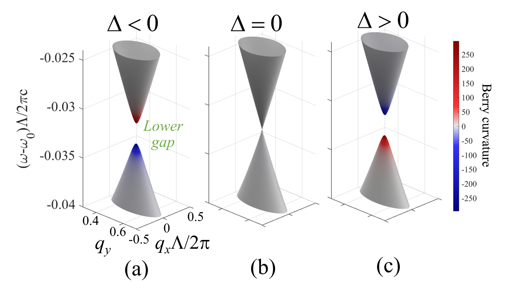
Figure S2: Engineering of the lower gap using two gratings which are slightly different. Three distinctive scenario are presented, corresponding to $\Delta=-0.05U$(a), $\Delta=0$(b) , $\Delta=0.05U$(c). Here the inter-layer coupling strength is fixed at $V=1.2U$

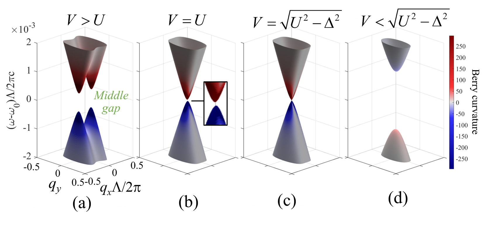
Figure S3: Engineering the middle gap by tuning the interlayer coupling strength $V$. Four distinctive scenario are presented, corresponding to $V=1.05U$(a), $V=U$(b) , $V=\sqrt{U^{2}-\Delta^{2}}$(c) and $V=0.95\sqrt{U^{2}-\Delta^{2}}$.

Remarkably, at $U=V$, the two Lateral Dirac cones merge together. The total winding number vanishes as expected  [41] which follows directy from (S3.28).

Appendix S4 Gap opening when $\Delta\neq 0$

S4.1 Band structures

One may demonstrate that all the Dirac degeneracies discussed in the previous section are lifted as soon as $\Delta\neq 0$ (i.e., the two gratings are different). The gap opening from upper, lower, and lateral Dirac points will be called upper, lower, and middle gaps (see Fig. 2). We are to find the effective Hamiltonian near each of the gaps.

S4.2 Upper and lower Dirac cones

We again use the notation

$$k_{x}=q_{x},\quad\tilde{k}_{y}=\frac{\left(q_{y}-1/2\right)\pi U}{v},$$ (S4.48)

and assume that $k_{x}$ and $\tilde{k}_{y}$ are small

$$k_{x},\tilde{k}_{y}\ll\frac{U}{v},\frac{V}{v}.$$ (S4.49)

We assume that $U$ and $V$ are at the same order of magnitude and $|\Delta|\ll U$. Upto the linear order in $k_{x},\tilde{k}_{y}$ we can rewrite the Hamiltonian (S1.3) as

$$H(k_{x},\tilde{k}_{y})=\omega_{0}+\left(\begin{matrix}vk_{x}&U+\Delta&-iV-\frac{V}{U}v\tilde{k}_{y}&0\\ U+\Delta&-vk_{x}&0&iV-\frac{V}{U}v\tilde{k}_{y}\\ iV-\frac{V}{U}vk_{y}&0&vk_{x}&U-\Delta\\ 0&-iV-\frac{V}{U}v\tilde{k}_{y}&U-\Delta&-vk_{x}\end{matrix}\right),$$ (S4.50)

Carrying out the same calculation steps as in the previous section, we obtain the effective Hamiltonian near the upper Dirac cone

$$H_{\mbox{upper}}\approx\omega_{0}+\sqrt{U^{2}+V^{2}}-v_{F}\vec{k}\cdot\vec{\sigma}+\Delta\sigma_{z}.$$ (S4.51)

with $\vec{k}\cdot\vec{\sigma}=k_{x}\sigma_{x}+\tilde{k}_{y}\sigma_{y}$, and the Fermi velocity $v_{F}$ is defined in Eq (S3.35). Similarly we found the effective Hamiltonian near the lower Dirac cone

$$H_{\mbox{lower}}\approx\omega_{0}-\sqrt{U^{2}+V^{2}}-v_{F}\vec{k}\cdot\vec{\sigma}+\Delta\sigma_{z}.$$ (S4.52)

We see that the (half) difference $\Delta$ between upper and lower intra coupling plays the role of effective Dirac mass. For $\Delta\neq 0$, the upper and lower Dirac points open energy gaps of $2\Delta$ as demonstrated Fig S2. Before and after the gaps close, the Berry curvatures change signs (see Figs S2 and 4), causing a topological phase transition.

Edge modes – We consider the case where we have a conjunction of two systems, one with $\Delta<0$ on the left and one with $\Delta>0$ on the right. The effective Dirac Hamiltonian (of upper and lower bands (S4.51),(S4.52)) will have opposite masses on different sides. We expect localized zero modes (similar to the bound state in the SSH model) at the junction to be observed. In the 2D hybrid momentum space, the localized state can be considered the chiral edge state with varying $k_{y}$. In this 2D hybrid mementum space, a single Dirac cone changes the sign of its Dirac mass across the junction, making a change $\Delta\Phi_{\rm Dirac}=\pm 1\times 2\pi(\Delta\mathcal{C}=\pm 1)$ in the total Berry flux (Chern number). Consequently, we expect to obtain one edge mode in the considering configuration at each of upper gap and lower gap (see Figs 3 and S8).

Remarks: In experimental setups, one cannot change the intra-layer coupling $U$ and the velocity $v$ independently. Consequently, a small change of $U$ may cause a change of $\Delta\omega_{0}$ of $\omega_{0}$ which is compatible with $\Delta$. The Hamiltonian (S4.50) corrected by these changes can be rewrite as

$$H(k_{x},\tilde{k}_{y})=\left(\begin{matrix}vk_{x}+\omega_{0}+\Delta\omega_{0}&U+\Delta&-iV-\frac{V}{U}v\tilde{k}_{y}&0\\ U+\Delta&-vk_{x}+\omega_{0}+\Delta\omega_{0}&0&iV-\frac{V}{U}v\tilde{k}_{y}\\ iV-\frac{V}{U}vk_{y}&0&vk_{x}+\omega_{0}-\Delta\omega_{0}&U-\Delta\\ 0&-iV-\frac{V}{U}v\tilde{k}_{y}&U-\Delta&-vk_{x}+\omega_{0}-\Delta\omega_{0}\end{matrix}\right),$$ (S4.53)

With the assumption that $\Delta,\Delta\omega_{0}\ll U,V$, we can obtain the leading order leading order of effective Hamiltonian for upper and lower Dirac cones

$$H_{upper}\approx\omega_{0}+\sqrt{U^{2}+V^{2}}-v_{F}\vec{k}\cdot\vec{\sigma}+(\Delta-\frac{U\Delta\omega_{0}}{\sqrt{U^{2}+V^{2}}})\sigma_{z}.$$ (S4.54)

$$H_{lower}\approx\omega_{0}-\sqrt{U^{2}+V^{2}}-v_{F}\vec{k}\cdot\vec{\sigma}+(\Delta-\frac{U\Delta\omega_{0}}{\sqrt{U^{2}+V^{2}}})\sigma_{z}.$$ (S4.55)

S4.3 Lateral Dirac cones

We again use the notation

$$k_{x}=q_{x},\quad k_{y}=\frac{\pi q_{y}V}{v}$$ (S4.56)

The Hamiltonian upto the first oder in $k_{y}$ is given by

$$H(k_{x},k_{y})=\omega_{0}+\left(\begin{matrix}vk_{x}&U+\Delta&V-ivk_{y}\frac{V}{U}&0\\ U+\Delta&-vk_{x}&0&V+ivk_{y}\\ V+ivk_{y}&0&vk_{x}&U-\Delta\\ 0&V-ivk_{y}\frac{V}{U}&U-\Delta&-vk_{x}\\ \end{matrix}\right).$$ (S4.57)

For $V>U$, and $\Delta\ll V-U$, we obtained two Dirac cones near $(k_{x}=+k_{D},k_{y}=0)$ and $(k_{x}=-k_{D},k_{y}=0)$. Consider first the effective theory near the Dirac cone at $(+k_{D},0)$. We then denote $\tilde{k}_{x}=k_{x}-k_{D}$ and obtain

$$H^{+}(\tilde{k}_{x},k_{y})=\omega_{0}+\left(\begin{matrix}v(\tilde{k}_{x}+k_{D})&U+\Delta&V-ivk_{y}\frac{V}{U}&0\\ U+\Delta&-v(\tilde{k}_{x}+k_{D})&0&V+ivk_{y}\\ V+ivk_{y}\frac{V}{U}&0&v(\tilde{k}_{x}+k_{D})&U-\Delta\\ 0&V-ivk_{y}&U-\Delta&-v(\tilde{k}_{x}+k_{D})\\ \end{matrix}\right)$$ (S4.58)

Ignoring the coupling of the middle bands to upper and lower band, one can write the effective Hamiltonian after performing a basis transformation as

$$H^{\mathbf{k}_{D}}_{c}(\tilde{k}_{x},k_{y},\Delta)=\omega_{0}+\left(\begin{array}[]{cc}-v\tilde{k}_{x}\frac{V^{2}-U^{2}}{V^{2}}-\frac{U\sqrt{V^{2}-U^{2}}}{V^{2}}\Delta&ivk_{y}+\tilde{v}\tilde{k}_{x}-\frac{V^{2}-U^{2}}{V^{2}}\Delta\\ -ivk_{y}+\tilde{v}\tilde{k}_{x}-\frac{V^{2}-U^{2}}{V^{2}}\Delta&v\tilde{k}_{x}\frac{V^{2}-U^{2}}{V^{2}}+\frac{U\sqrt{V^{2}-U^{2}}}{V^{2}}\Delta\\ \end{array}\right).$$ (S4.59)

Noticing that with the condition $\Delta\ll V-U\ll U,V$, and therefore

$$\tilde{v}\tilde{k}_{x}\gg v\tilde{k}_{x}\frac{V^{2}-U^{2}}{V^{2}},\quad|\frac{U\sqrt{V^{2}-U^{2}}}{2V^{2}}\Delta|\gg|\frac{V^{2}-U^{2}}{V^{2}}\Delta|,$$ (S4.60)

we arrive at the effective Hamiltonian

$$H^{+}_{c}(\tilde{k}_{x},k_{y},\Delta)\approx\omega_{0}+\left(\begin{array}[]{cc}-\frac{U\sqrt{V^{2}-U^{2}}}{V^{2}}\Delta&ivk_{y}+\tilde{v}\tilde{k}_{x}\\ -ivk_{y}+\tilde{v}\tilde{k}_{x}&\frac{U\sqrt{V^{2}-U^{2}}}{V^{2}}\Delta\\ \end{array}\right)$$ (S4.61)

We can repeat the similar calculation for the effective Hamiltonian near the Dirac cone $(-k_{D},0)$. With the notation

$$\tilde{k}_{x}=k_{x}+k_{D},$$ (S4.62)

we arrive at an effective Hamiltonian at the Dirac cone $(-k_{D},0)$

$$H^{-}_{c}(\tilde{k}_{x},k_{y},\Delta)\approx\omega_{0}+\left(\begin{array}[]{cc}\frac{U\sqrt{V^{2}-U^{2}}}{V^{2}}\Delta&ivk_{y}-\tilde{v}\tilde{k}_{x}\\ -ivk_{y}-\tilde{v}\tilde{k}_{x}&-\frac{U\sqrt{V^{2}-U^{2}}}{V^{2}}\Delta\\ \end{array}\right)$$ (S4.63)

Comparing (S4.61) and (S4.63), we see that two Dirac cones have the opposite winding number since the coefficient of $k_{y}$ changes its sign and also have the opposite Dirac mass. Consequently, they have the same Berry curvature when the energy gaps are open with at a finite value of $\Delta$. Each lateral Dirac cones contribute a total Berry flux $\Phi_{\rm Dirac}=\pm\pi$; therefore, the contribution of lateral Dirac cones to the change of the total Berry flux of the center bands are $\Delta\Phi_{\rm Dirac}=\pm 2\pi$ when the energy gap is opened at a finite $\Delta$.

Edge modes by connecting $\Delta<0$ and $\Delta>0$ – We consider the case where we have the conjunction of two systems, one with $\Delta<0$ on the left and one with $\Delta>0$ on the right. We have a change of total Berry flux (Chern number) $\Delta\Phi=\pm 2\times 2\pi$ $(\Delta\mathcal{C}=\pm 2)$ across the junction. Consequently, we expect to have two edge modes near the boundary (see Figs 3 and S9).

Dirac cones merging – If we keep a fixed value of $\Delta\ll U,V$ and change the ratio $V/U$, the two lateral Dirac cones merge at approximately $U\approx V$ . When $U\approx V$, we can derive the effective Hamiltonian of the two middle bands near $\vec{k}=(0,0)$ as

$$H_{c}^{\rm eff}(k_{x},k_{y})\approx\omega_{0}+\left(\begin{matrix}U-\sqrt{V^{2}+\Delta^{2}}+\frac{v^{2}k_{x}^{2}}{2U}&\frac{ivk_{y}V-vk_{x}\Delta}{\sqrt{V^{2}+\Delta^{2}}}\\ \frac{-ivk_{y}V-vk_{x}\Delta}{\sqrt{V^{2}+\Delta^{2}}}&-U+\sqrt{V^{2}+\Delta^{2}}-\frac{v^{2}k_{x}^{2}}{2U}\end{matrix}\right).$$ (S4.64)

At $\Delta=0$, we recover the effective Hamiltonian (S3.44) after a change of basis. The effective Hamiltonian (S4.64), at small $k_{x}$, is an effective Hamiltonian of a Dirac cone with the Dirac mass $U-\sqrt{V^{2}+\Delta^{2}}$ and the winding number depends on the sign of $\Delta$. At this configuration, the Dirac mass of this center cone is much smaller than the Dirac masses of the upper and the lower Dirac cones.

Edge modes by connecting $\Gamma<0$ and $\Gamma>0$ – The energy gap between the middle bands closed at $\Gamma=U-\sqrt{V^{2}+\Delta^{2}}$. Consequently, the total Berry flux (Chern number) changes $\Delta\Phi=\pm 1\times 2\pi$ $(\Delta\mathcal{C}=\pm 1)$ when $\Gamma$ switches its sign (see Fig. S3 and Fig. 2). We then expect one edge mode at the middle gap when connecting two systems with $\Gamma<0$ and $\Gamma>0$ that share the same sign of $\Delta$ (see Fig. S10).

Remark: Some comments are in order, with the appearance of $\Delta\omega_{0}$, the explicit effective Hamiltonian of lateral Dirac cones will be much more complicated; however, the conclusions about the total Berry flux and the number of edge modes are unchanged.

Appendix S5 Supplemental Figures

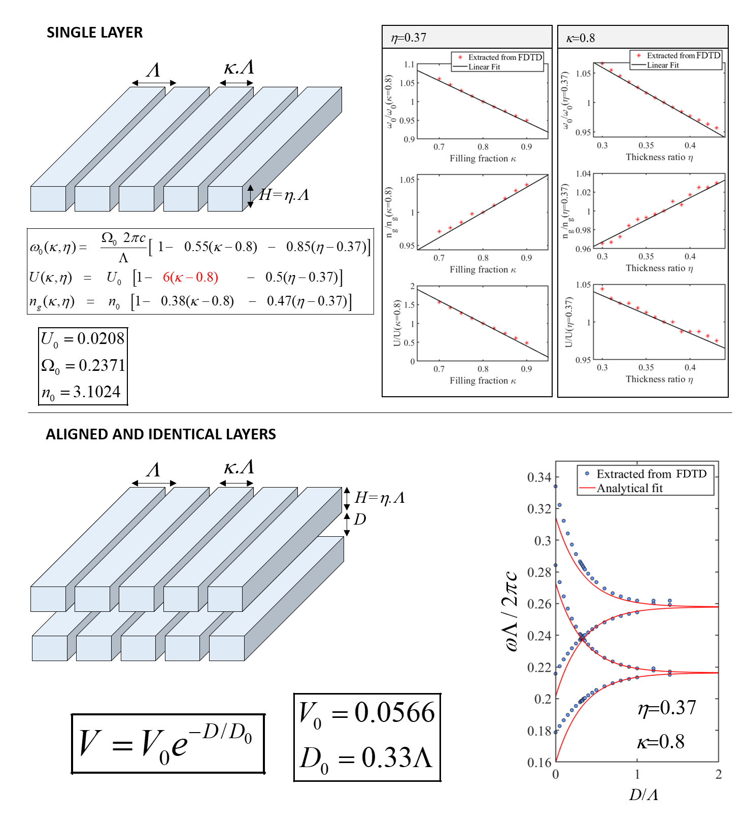
Figure S4: Parameter retrievals for the effective Hamiltonian from FDTD simulations. Upper Panels: the simulations for single layer grating are used to obtain the dependence of $\omega_{0}$, $U$ and $n_{g}$ as functions of the filling fraction $\kappa$ and thickness ratio $\eta$. These parameters are extracted by fitting the two band dispersion with the Hamiltonian $H_{single}=\omega_{0}\mathbb{I}+\sigma_{x}U+\sigma_{z}q_{x}/n_{g}$. Lower Panels: the simulations for aligned and identical gratings at $q_{x}=0$ are used to obtain the dependence of $V$ as functions of the distance $D$ separating the two layers. The exponential decay law of $V$ is obtained by fitting the four band edges $\omega_{0}+U+V$,$\omega_{0}+U-V$,$\omega_{0}-U+V$ and $\omega_{0}-U-V$ at different distance $D$. Here the values of $U$ and $\omega_{0}$ are already known thanks to the retrievals from the single layer simulationss.

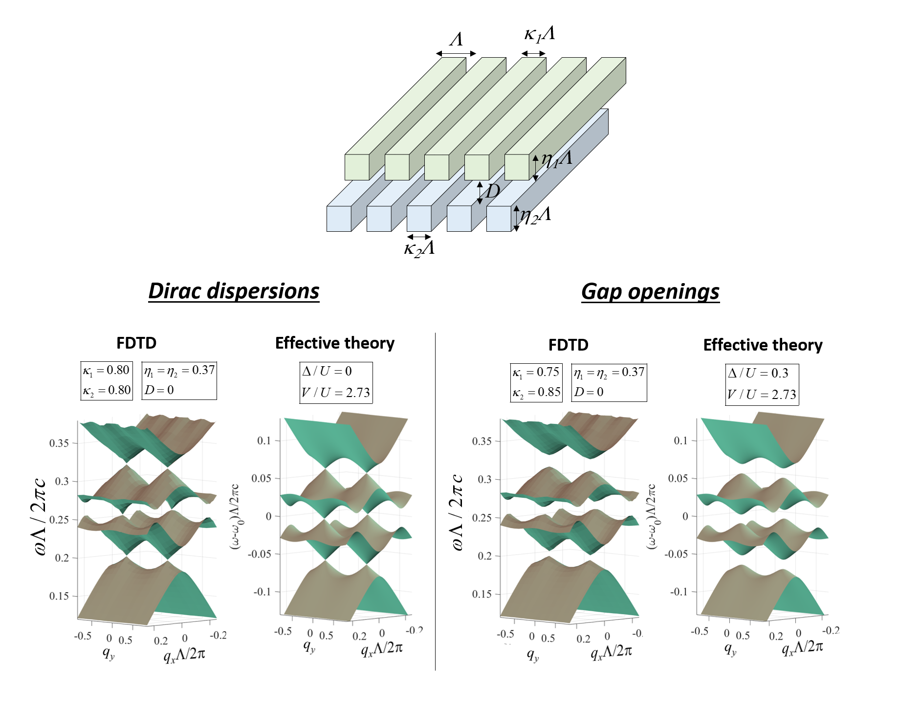
Figure S5: Comparison between bulk band structure obtained by FDTD simulations and the one calculated by the effective theory using the retrieved parameters shown in Fig. S4. Here the simulated band structure are only shown in the vicinity of $q_{x}=0$ (i.e. X point of the 1D Brillouin zone) since the effective theory only valids in this region.

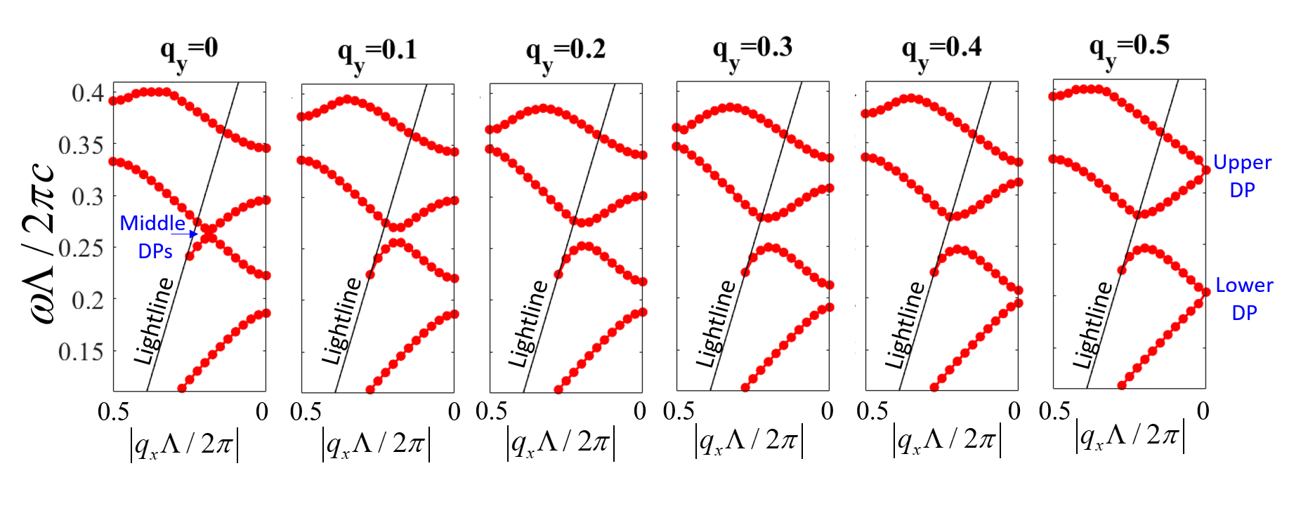
Figure S6: Full band structure of the bulk corresponds given by FDTD simulations for the case $\kappa_{1}=\kappa_{2}=0.8$, $\eta_{1}=\eta_{2}=0.37$ and $D=0$. It shows that while the lower Dirac point and the middle Dirac points are well spectrally isolated, it is not the case for the upper Dirac point since there are bulk bands at the same energy at high wave vector.

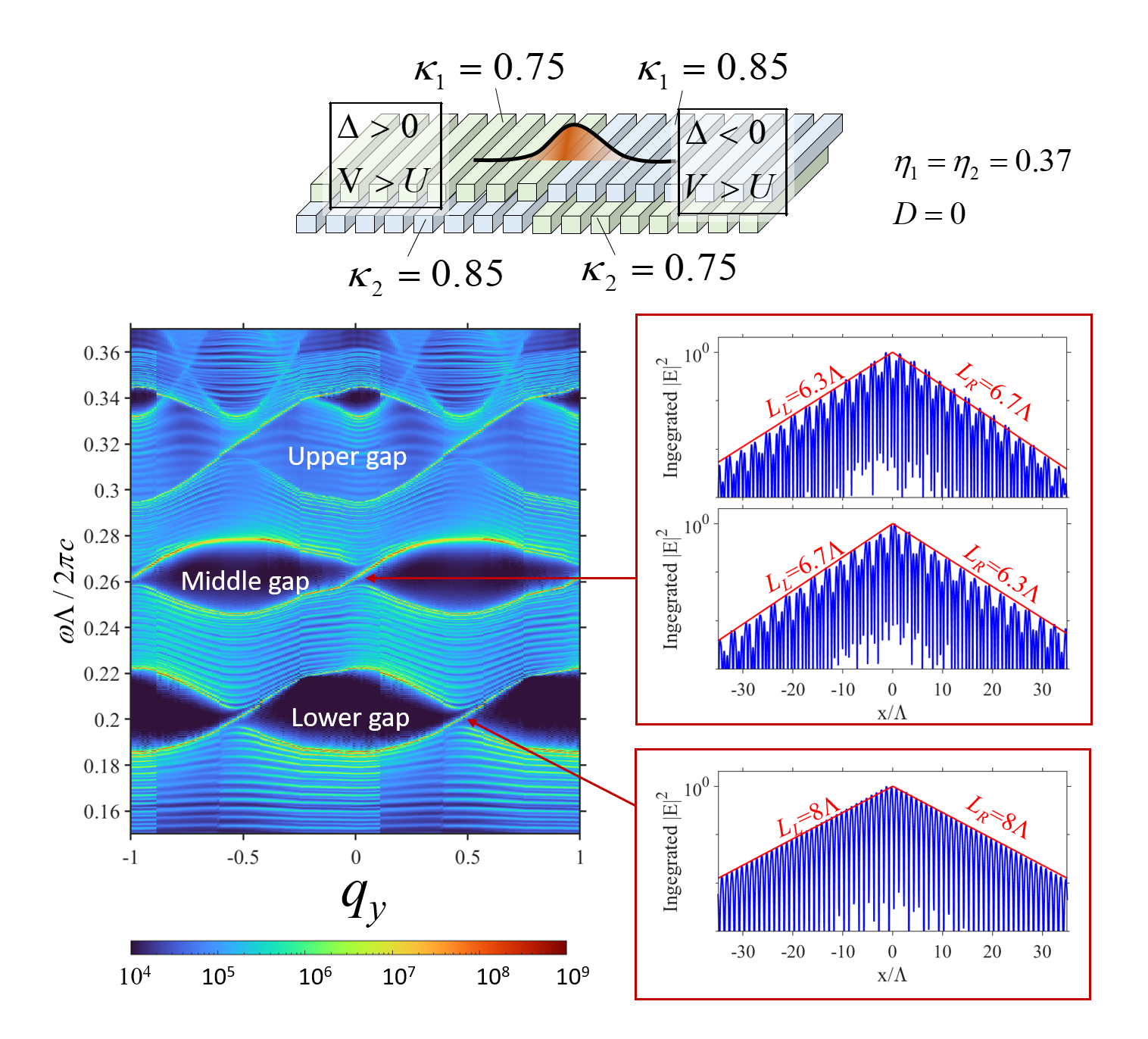
Figure S7: Topological edge states from the “heterostructure” consists of two topological phases having opposite $\Delta$ value. The design corresponds to the one presented in the Fig. 3 of the main text. Here the spectra along $q_{y}$, numerically calculated by FDTD, is shown for within two periods of $q_{y}$ and with the full energy scale of the four bulk bands. There are bulk bands that are not described by the effective theory cross the upper gap. Thus only the Middle gap and Lower gap are considered for edgestates.

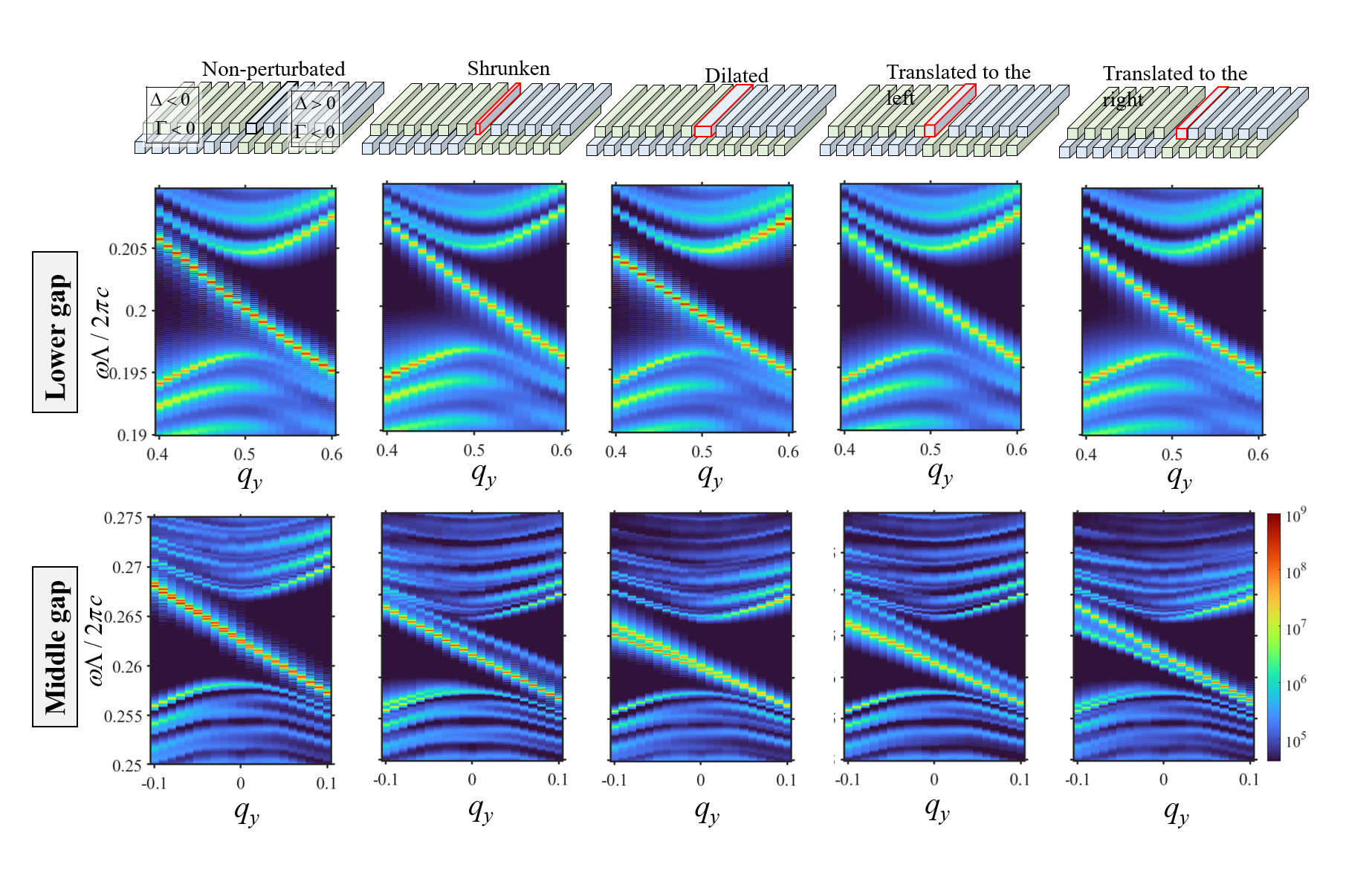
Figure S8: The robustness of the chirality of the topological edge states discussed in Fig. 3 in the main text and in Fig. S7, but here the interface is strongly perturbed by modifying either the size or the position of the first rod in the upper-right grating. These results show that the: i) The chirality is topologically protected against perturbations, ii) The degeneracy lifting of the two edge states in the middle gap depends strongly on the interface, i.e. boundary conditions.

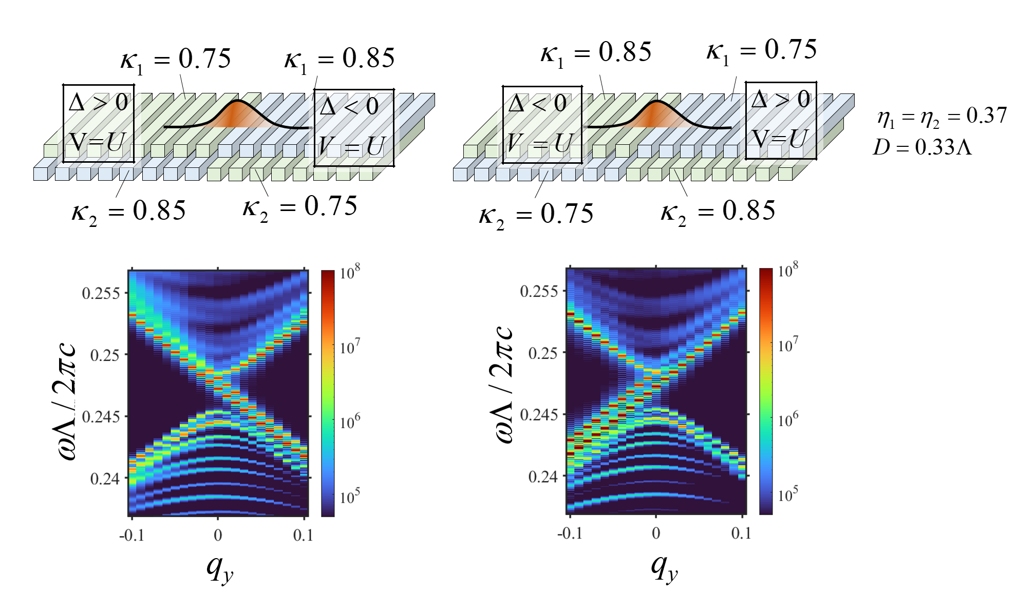
Figure S9: Topological edge states within the middle gap from the “heterostructure” consists of two topological phases having opposite $\Delta$ value. Here the design corresponds to the special case $V=U$ at which we have the merging of the two mini-middle gaps (see Fig. S3b for the bulk band structure).When $U<\sqrt{V^{2}+\Delta^{2}}$, topologically, the change of the total Berry flux when switching the sign of $\Delta$ equals to the change when switching the sign of the Dirac masses of the two lateral Dirac cones. Therefore the difference of total the Berry flux between the left and the right sides is $4\pi$, which also implies the difference of the Chern number $\Delta\mathcal{C}\pm 2$ the left and the right sides Consequently, we expect two edge modes in the considering configuration.

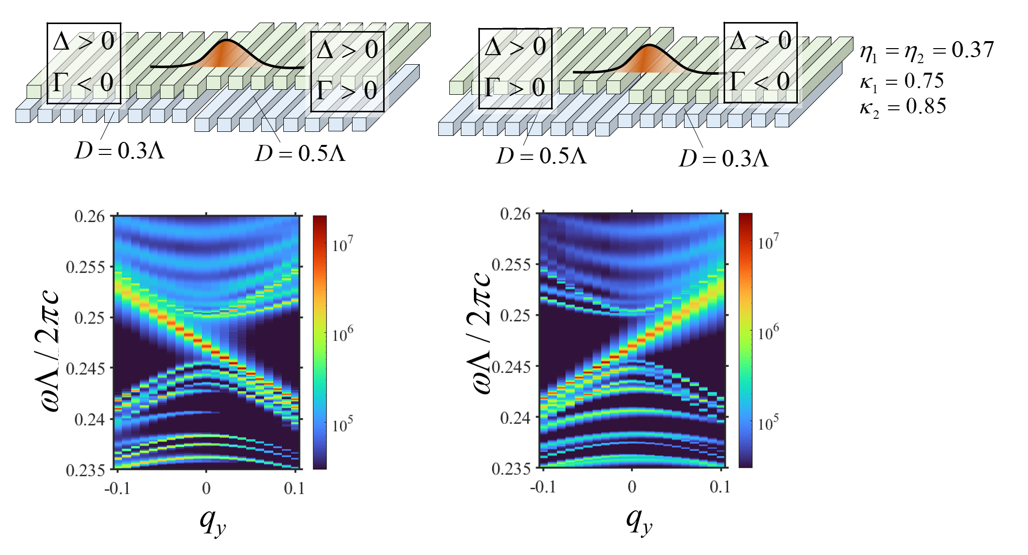
Figure S10: Topological edge states within the middle gap from the “heterostructure” consists of two topological phases having opposite $\Gamma$ value. From Eq (S4.64), closed to the value $\Gamma=0$, the effective Hamiltonian of the middle bands is the Dirac Hamiltonian with the Dirac mass $\Gamma$. When we switch the sign of $\Gamma$, the change of the total Berry flux is $\pm 2\pi$, which also implies the difference of the Chern number $\Delta\mathcal{C}\pm 1$ the left and the right sides. Consequently, there should be only one edge mode.

References

- Onsager [1949] L. Onsager, Statistical hydrodynamics, Il Nuovo Cimento 6, 279 (1949).
- Feynman [1955] R. Feynman, Chapter ii application of quantum mechanics to liquid helium (Elsevier, 1955) pp. 17–53.
- Bogdanov and Rößler [2001] A. N. Bogdanov and U. K. Rößler, Chiral Symmetry Breaking in Magnetic Thin Films and Multilayers, Phys. Rev. Lett. 87, 037203 (2001).
- Mühlbauer et al. [2009] S. Mühlbauer, B. Binz, F. Jonietz, C. Pfleiderer, A. Rosch, A. Neubauer, R. Georgii, and P. Böni, Skyrmion Lattice in a Chiral Magnet, Science 323, 915 (2009).
- Barthelemy et al. [1985] A. Barthelemy, S. Maneuf, and C. Froehly, Propagation soliton et auto-confinement de faisceaux laser par non linearité optique de kerr, Optics Communications 55, 201 (1985).
- Segev et al. [1992] M. Segev, B. Crosignani, A. Yariv, and B. Fischer, Spatial solitons in photorefractive media, Phys. Rev. Lett. 68, 923 (1992).
- Klitzing et al. [1980] K. V. Klitzing, G. Dorda, and M. Pepper, New Method for High-Accuracy Determination of the Fine-Structure Constant Based on Quantized Hall Resistance, Phys. Rev. Lett. 45, 494 (1980).
- Thouless et al. [1982] D. J. Thouless, M. Kohmoto, M. P. Nightingale, and M. den Nijs, Quantized hall conductance in a two-dimensional periodic potential, Phys. Rev. Lett. 49, 405 (1982).
- Haldane [1988] F. D. M. Haldane, Model for a quantum hall effect without landau levels: Condensed-matter realization of the "parity anomaly", Phys. Rev. Lett. 61, 2015 (1988).
- Kane and Mele [2005] C. L. Kane and E. J. Mele, Quantum spin hall effect in graphene, Phys. Rev. Lett. 95, 226801 (2005).
- Kane and Mele [2005] C. L. Kane and E. J. Mele, Z2 Topological Order and the Quantum Spin Hall Effect, Phys. Rev. Lett. 95, 146802 (2005).
- Pankratov et al. [1987] O. A. Pankratov, S. V. Pakhomov, and B. A. Volkov, Supersymmetry in heterojunctions: Band-inverting contact on the basis of Pb 1□xSn xTe and Hg 1□xCd xTe, Solid State Communications 61, 93 (1987).
- Bernevig and Zhang [2006] B. A. Bernevig and S.-C. Zhang, Quantum spin hall effect, Phys. Rev. Lett. 96, 106802 (2006).
- König et al. [2007] M. König, S. Wiedmann, C. Brüne, A. Roth, H. Buhmann, L. W. Molenkamp, X.-L. Qi, and S.-C. Zhang, Quantum Spin Hall Insulator State in HgTe Quantum Wells, Science 318, 766 (2007).
- Fu and Kane [2007] L. Fu and C. L. Kane, Topological insulators with inversion symmetry, Phys. Rev. B 76, 045302 (2007).
- Hsieh et al. [2008] D. Hsieh, D. Qian, L. Wray, Y. Xia, Y. S. Hor, R. J. Cava, and M. Z. Hasan, A topological Dirac insulator in a quantum spin Hall phase, Nature (London) 452, 970 (2008).
- Ozawa et al. [2019] T. Ozawa, H. M. Price, A. Amo, N. Goldman, M. Hafezi, L. Lu, M. C. Rechtsman, D. Schuster, J. Simon, O. Zilberberg, and I. Carusotto, Topological photonics, Rev. Mod. Phys. 91, 015006 (2019).
- Wang et al. [2009] Z. Wang, Y. Chong, J. D. Joannopoulos, and M. Soljacic, Observation of unidirectional backscattering-immune topological electromagnetic states, Nature 461, 772 (2009).
- Skirlo et al. [2015] S. A. Skirlo, L. Lu, Y. Igarashi, Q. Yan, J. Joannopoulos, and M. Soljacic, Experimental observation of large chern numbers in photonic crystals, Phys. Rev. Lett. 115, 253901 (2015).
- Skirlo et al. [2014] S. A. Skirlo, L. Lu, and M. Soljacic, Multimode one-way waveguides of large chern numbers, Phys. Rev. Lett. 113, 113904 (2014).
- Hafezi et al. [2011] M. Hafezi, E. A. Demler, M. D. Lukin, and J. M. Taylor, Robust optical delay lines with topological protection, Nature Physics 7, 907 (2011).
- Rechtsman et al. [2013] M. C. Rechtsman, J. M. Zeuner, Y. Plotnik, Y. Lumer, D. Podolsky, F. Dreisow, S. Nolte, M. Segev, and A. Szameit, Photonic Floquet topological insulators, Nature 496, 196 (2013).
- Boada et al. [2012] O. Boada, A. Celi, J. I. Latorre, and M. Lewenstein, Quantum simulation of an extra dimension, Phys. Rev. Lett. 108, 133001 (2012).
- Mei et al. [2012] F. Mei, S.-L. Zhu, Z.-M. Zhang, C. H. Oh, and N. Goldman, Simulating topological insulators with cold atoms in a one-dimensional optical lattice, Phys. Rev. A 85, 013638 (2012).
- Celi et al. [2014a] A. Celi, P. Massignan, J. Ruseckas, N. Goldman, I. B. Spielman, G. Juzeliūnas, and M. Lewenstein, Synthetic gauge fields in synthetic dimensions, Phys. Rev. Lett. 112, 043001 (2014a).
- Price et al. [2015] H. M. Price, O. Zilberberg, T. Ozawa, I. Carusotto, and N. Goldman, Four-dimensional quantum hall effect with ultracold atoms, Phys. Rev. Lett. 115, 195303 (2015).
- Regensburger et al. [2012] A. Regensburger, C. Bersch, M.-A. Miri, G. Onishchukov, D. N. Christodoulides, and U. Peschel, Parity–time synthetic photonic lattices, Nature 488, 167 (2012).
- Dutt et al. [2020] A. Dutt, M. Minkov, I. Williamson, and S. Fan, Higher-order topological insulators in synthetic dimensions, Light: Science & Applications 9, 131 (2020).
- Yuan et al. [2016a] L. Yuan, Y. Shi, and S. Fan, Photonic gauge potential in a system with a synthetic frequency dimension, Opt. Lett. 41, 741 (2016a).
- Buddhiraju et al. [2021] S. Buddhiraju, A. Dutt, M. Minkov, I. A. D. Williamson, and S. Fan, Arbitrary linear transformations for photons in the frequency synthetic dimension, Nat. Comm. 12, 10.1038/s41467-021-22670-7 (2021).
- Yuan et al. [2018] L. Yuan, Q. Lin, M. Xiao, and S. Fan, Synthetic dimension in photonics, Optica 5, 1396 (2018).
- Segev and Bandres [2021] M. Segev and M. A. Bandres, Topological photonics: Where do we go from here?, Nanophotonics 10, 425 (2021).
- Celi et al. [2014b] A. Celi, P. Massignan, J. Ruseckas, N. Goldman, I. Spielman, G. Juzeliūnas, and M. Lewenstein, Synthetic Gauge Fields in Synthetic Dimensions, Phys. Rev. Lett. 112, 043001 (2014b).
- Yuan et al. [2016b] L. Yuan, Y. Shi, and S. Fan, Photonic gauge potential in a system with a synthetic frequency dimension, Opt. Lett. 41, 741 (2016b).
- Yuan et al. [2021] L. Yuan, A. Dutt, and S. Fan, Synthetic frequency dimensions in dynamically modulated ring resonators, APL Photonics 6, 071102 (2021).
- Lustig et al. [2019] E. Lustig, S. Weimann, Y. Plotnik, Y. Lumer, M. A. Bandres, A. Szameit, and M. Segev, Photonic topological insulator in synthetic dimensions, Nature 567, 356 (2019).
- Zilberberg et al. [2018] O. Zilberberg, S. Huang, J. Guglielmon, M. Wang, K. P. Chen, Y. E. Kraus, and M. C. Rechtsman, Photonic topological boundary pumping as a probe of 4D quantum Hall physics, Nature 553, 59 (2018).
- Ozawa et al. [2016] T. Ozawa, H. M. Price, N. Goldman, O. Zilberberg, and I. Carusotto, Synthetic dimensions in integrated photonics: From optical isolation to four-dimensional quantum Hall physics, Physical Review A 93, 043827 (2016).
- Chiu et al. [2016] C.-K. Chiu, J. C. Y. Teo, A. P. Schnyder, and S. Ryu, Classification of topological quantum matter with symmetries, Rev. Mod. Phys. 88, 035005 (2016).
- Montambaux et al. [2009] G. Montambaux, F. Piéchon, J.-N. Fuchs, and M. O. Goerbig, Merging of dirac points in a two-dimensional crystal, Phys. Rev. B 80, 153412 (2009).
- Goerbig and Montambaux [2017] M. Goerbig and G. Montambaux, Dirac fermions in condensed matter and beyond, in Dirac Matter, edited by B. Duplantier, V. Rivasseau, and J.-N. Fuchs (Springer International Publishing, Cham, 2017) pp. 25–53.
- Huang et al. [2016] S.-M. Huang, S.-Y. Xu, I. Belopolski, C.-C. Lee, G. Chang, T.-R. Chang, B. Wang, N. Alidoust, G. Bian, M. Neupane, D. Sanchez, H. Zheng, H.-T. Jeng, A. Bansil, T. Neupert, H. Lin, and M. Z. Hasan, New type of Weyl semimetal with quadratic double Weyl fermions, Proc. Nat. Acad. Sci. 113, 1180 (2016).
- Dóra et al. [2013] B. Dóra, I. F. Herbut, and R. Moessner, Coupling, merging, and splitting Dirac points by electron-electron interaction, Phys. Rev. B 88, 075126 (2013).
- Montambaux et al. [2018] G. Montambaux, L.-K. Lim, J.-N. Fuchs, and F. Piéchon, Winding Vector: How to Annihilate Two Dirac Points with the Same Charge, Phys. Rev. Lett. 121, 256402 (2018).
- Nguyen et al. [2018] H. S. Nguyen, F. Dubois, T. Deschamps, S. Cueff, A. Pardon, J.-L. Leclercq, C. Seassal, X. Letartre, and P. Viktorovitch, Symmetry breaking in photonic crystals: On-demand dispersion from flatband to dirac cones, Phys. Rev. Lett. 120, 066102 (2018).
- Nguyen et al. [2021] D. X. Nguyen, X. Letartre, E. Drouard, P. Viktorovitch, H. C. Nguyen, and H. S. Nguyen, Magic configurations in moiré superlattice of bilayer photonic crystal: Almost-perfect flatbands and unconventional localization (2021), arXiv:2104.12774 [physics.optics] .
- [47] See Supplemental Materials at (link) for derivation details of the topology of the band structures, supplemental FDTD simulations of the bulks (band structures, parameter retrieval), edge states (different chiralities, robustness).
- Girvin and Yang [2019] S. M. Girvin and K. Yang, Modern Condensed Matter Physics (Cambridge University Press, 2019).
- Note [1] Here is some subtlety generally encountered in computing the total Berry flux: the effective Hamiltonian is written for non-compactly extending , but is really only valid for small . The actual momentum space of the system is compact. However, assuming the gap does not close elsewhere far from the touching points around small , the analysis of the local contribution to total Berry flux can be used to infer the topological transitions of the total bands.
- St-Jean et al. [2017] P. St-Jean, V. Goblot, E. Galopin, A. Lemaître, T. Ozawa, L. Le Gratiet, I. Sagnes, J. Bloch, and A. Amo, Lasing in topological edge states of a one-dimensionallattice, Nature Photonics 11, 651 (2017).
- Ota et al. [2018] Y. Ota, R. Katsumi, K. Watanabe, S. Iwamoto, and Y. Arakawa, Topological photonic crystal nanocavity laser, Communications Physics 1, 86 (2018).
- Zhao et al. [2018] H. Zhao, P. Miao, M. H. Teimourpour, S. Malzard, R. El-Ganainy, H. Schomerus, and L. Feng, Topological hybrid silicon microlasers, Nature Communications 9, 981 (2018).
- Han et al. [2019] C. Han, M. Lee, S. Callard, C. Seassal, and H. Jeon, Lasing at topological edge states in a photonic crystal L3 nanocavity dimer array, Light: Science & Applications 8, 40 (2019).
- Ashcroft and Mermin [1976] N. Ashcroft and N. Mermin, Solid State Physics (Saunders College, Philadelphia, 1976).
- Bernevig [2013] B. A. Bernevig, Topological Insulators and Topological Superconductors (Princeton University Press, 2013).