Mixed Models and Shrinkage Estimation for Balanced and Unbalanced Designs

Abstract

The known connection between shrinkage estimation, empirical Bayes, and mixed effects models is explored and applied to balanced and unbalanced designs in which the responses are correlated. As an illustration, a mixed model is proposed for predicting the outcome of English Premier League games that takes into account both home and away team effects. Results based on empirical best linear unbiased predictors obtained from fitting mixed linear models are compared with fully Bayesian predictors that utilize prior information from the previous season.
Keywords: BLUP, EBLUP, empirical Bayes, football pools, MAP estimation

1 Introduction

The famous result due to Charles Stein (Stein, 1955) concerning the inadmissibility of the maximum likelihood estimator of a multivariate normal mean with respect to squared error loss has generated a lot of interest in shrinkage estimation in the decades since. In particular, the connection to empirical Bayes estimation first noted by Efron and Morris (1973) means that the benefits of shrinkage estimation can be obtained using mixed effects models and, specifically, linear mixed effects models in many situations.

In this paper we consider estimation based on a $t\times n$ data matrix, ${\mathbf{Y}}$, where, initially, we assume a data generating mechanism in which the columns of ${\mathbf{Y}}$, denoted by ${\mathbf{y}}_{j}$, $j=1,\ldots,n$, are independent Gaussian vectors with mean vector $\mu$ and covariance matrix $\Sigma$. In some cases, such as a balanced incomplete block design (BIBD), some of the elements of each column of the data matrix may be missing. In this case, and if the data is unbalanced, the value of $\mu$ varies with $j$ (see Section 4 for a case study).

The classical Stein estimation setting concerns the complete data case in which ${\mbox{\boldmath$\Sigma$}}=\sigma^{2}{\mathbf{I}}$. In this setting Stein (1955) showed that the maximum likelihood estimator (MLE) for $\mu$, $\widehat{{\mbox{\boldmath$\mu$}}}^{MLE}=\bar{{\mathbf{y}}}$, is inadmissible with respect to total squared error loss for $t\geq 3$, where $\bar{{\mathbf{y}}}={\mathbf{Y}}{\mbox{\boldmath$1$}}/n=(\bar{y}_{1\cdot},\ldots,\bar{y}_{t\cdot})^{T}$ denotes the mean of the rows of the data matrix.

We review the classical setting and the connections to empirical Bayes and linear mixed models in Section 2. Section 3 concerns the extension of the classical results to the randomized complete blocks and balanced incomplete block design settings in which responses within blocks are correlated. In Section 4 we propose a linear mixed model for predicting the outcomes (goal differences) of individual games in the English Premier League (EPL) which takes into account both home and away team effects. In Section 5 we discuss how prior information from previous EPL seasons can be incorporated into the modeling strategy. We conclude in Section 6 with some discussion.

2 Classical Stein Shrinkage Estimation

Suppose that ${\mathbf{y}}_{j}\sim N({\mbox{\boldmath$\mu$}},\sigma^{2}_{e}{\mathbf{I}}_{t})$. James and Stein (1961) showed that the estimator

$$\widehat{{\mbox{\boldmath$\mu$}}}^{JS}=\left(1-\frac{\sigma^{2}_{e}/n}{S_{0}/(t-2)}\right)\bar{{\mathbf{y}}}\,,$$ (1)

where $S_{0}=||\bar{{\mathbf{y}}}||^{2}$, dominates the MLE, $\bar{{\mathbf{y}}}$, in terms of squared error loss for all values of $\mu$. The JS estimator shrinks the sample mean components towards zero (provided the multiplying factor in (1) is positive and less than 1). A modification, known as Lindley’s estimate (or JSL) is to shrink towards the overall mean $\bar{y}_{\cdot\cdot}={\mbox{\boldmath$1$}}_{t}^{T}{\mathbf{Y}}{\mbox{\boldmath$1$}}_{n}/tn$,

$$\widehat{{\mbox{\boldmath$\mu$}}}^{JSL}={\mbox{\boldmath$1$}}_{t}\bar{y}_{\cdot\cdot}+\left(1-\frac{\sigma^{2}_{e}/n}{S/(t-3)}\right)(\bar{{\mathbf{y}}}-{\mbox{\boldmath$1$}}_{t}\bar{y}_{\cdot\cdot})\,,$$ (2)

where $S=||\bar{{\mathbf{y}}}-{\mbox{\boldmath$1$}}_{t}\bar{y}_{\cdot\cdot}||^{2}$. An unbiased estimate of $\sigma^{2}_{e}$ is given by $\widehat{\sigma}^{2}_{e}=\sum_{i=1}^{t}\sum_{j=1}^{n}(y_{ij}-\bar{y}_{i\cdot})^{2}/t(n-1)$, and the ratio, $\widehat{\sigma}^{2}_{e}/\sigma^{2}_{e}$, is distributed as $\chi^{2}_{t(n-1)}/t(n-1)$ independently of $\bar{\mathbf{y}}$. This fact can be used to show that the JSL estimator still dominates the MLE even when $\sigma^{2}_{e}$ is estimated (see e.g., Lehmann and Casella, 1998, chapter 5).

Efron and Morris (1973) showed that shrinkage estimators such as (1) and (2) can be motivated from an empirical Bayes (EB) perspective. Specifically, suppose that, conditionally on $\mu$, the columns of ${\mathbf{Y}}$ are iid $N({\mbox{\boldmath$\mu$}},\sigma^{2}_{e}{\mathbf{I}}_{t})$. This is the same distributional assumption made above, but now, in addition, suppose that $\mu$ is also random, and that ${\mbox{\boldmath$\mu$}}\sim N({\mbox{\boldmath$0$}},\sigma^{2}_{\mu}{\mathbf{I}}_{t})$. Then the posterior mean of $\mu$ given the data matrix, ${\mathbf{Y}}$, is given by

$$E({\mbox{\boldmath$\mu$}}|{\mathbf{Y}})=\left(1-\frac{\sigma^{2}_{e}/n}{\sigma^{2}_{\mu}+\sigma^{2}_{e}/n}\right)\bar{{\mathbf{y}}}\,.$$

Under these modeling assumptions, an unbiased estimator of the the denominator, $\sigma^{2}_{\mu}+\sigma^{2}_{e}/n$, is given by $S_{0}/t$ resulting in an estimator the same as (1) except for the substitution of $t$ in place of $t-2$.

An alternative 3-parameter EB model sets ${\mbox{\boldmath$\mu$}}={\mbox{\boldmath$1$}}_{t}\bar{\mu}+{\mathbf{u}}$, where $\bar{\mu}={\mbox{\boldmath$1$}}_{t}^{T}E({\mbox{\boldmath$\mu$}})/t$ is a fixed scalar parameter and ${\mathbf{u}}\sim N({\mbox{\boldmath$0$}}_{t},\sigma^{2}_{u}{\mathbf{I}}_{t})$. In this case, the posterior mean of $\mu$ given the data matrix is given by

$$E({\mbox{\boldmath$\mu$}}|{\mathbf{Y}})={\mbox{\boldmath$1$}}_{t}\bar{\mu}+\left(1-\frac{\sigma^{2}_{e}/n}{\sigma^{2}_{u}+\sigma^{2}_{e}/n}\right)(\bar{{\mathbf{y}}}-{\mbox{\boldmath$1$}}_{t}\bar{\mu})\,.$$ (3)

Under these modeling assumptions, unbiased estimators for $\bar{\mu}$, $\sigma^{2}_{e}$ and $\sigma^{2}_{u}+\sigma^{2}_{e}/n$ are given by $\bar{y}_{\cdot\cdot}$, $\widehat{\sigma}^{2}_{e}$ and $S/(t-1)$. Substituting these values results in an estimator the same as (2) except for the use of $t-1$ in place of $t-3$. An equivalent specification of this second EB model using mixed model notation is

$$y_{ij}=\bar{\mu}+u_{i}+e_{ij}\,,$$ (4)

where $e_{ij}\sim\mbox{ iid }N(0,\sigma^{2}_{e})$ independently of $u_{i}\sim\mbox{ iid }N(0,\sigma^{2}_{u})$. It follows that an EB version of the JSL estimator can be obtained by fitting (4) using standard mixed model software and extracting the empirical best linear unbiased predictors (EBLUPs) for $\mu+u_{i}$, $i=1,\ldots,t$. In particular, the mixed model fits in this paper were obtained using the lmer function from the lme4 package in R (R Core Team, 2021), with the method=REML option.

3 Randomized Blocks Designs

In this section we relax the distributional assumptions to allow for correlation between responses. Specifically, suppose that ${\mathbf{y}}_{j}\sim\mbox{ iid }N({\mbox{\boldmath$\mu$}},\sigma^{2}_{e}{\mathbf{I}}_{t}+\sigma^{2}_{b}{\mathbf{J}}_{t})$, where ${\mathbf{J}}_{t}$ denotes a $t\times t$ matrix of ones. This distributional assumption is the same as that encountered in a classical randomized complete blocks design (RCBD) with one complete set of treatments per block; see e.g. Cochran and Cox (1957, chapter 4), whereby

$$y_{ij}=\bar{\mu}+\upsilon_{i}+b_{j}+e_{ij},$$ (5)

where $\upsilon_{i}$ is the deviation of the $i$th ‘treatment’ mean from the overall mean, the $b_{j}$’s are random ‘block’ effects with $b_{j}\sim\mbox{ iid }N(0,\sigma^{2}_{b})$ independently of the random ‘errors’ $e_{ij}\sim\mbox{ iid }N(0,\sigma^{2}_{e})$.

The normality and independence assumptions together imply that the MLE for $\mu$ is a solution of the generalized least squares (GLS) estimating equation

$${\mbox{\boldmath$0$}}=\sum_{j=1}^{n}(\sigma_{e}^{2}{\mathbf{I}}_{t}+\sigma_{b}^{2}{\mathbf{J}}_{t})^{-1}({\mathbf{y}}_{j}-{\mbox{\boldmath$\mu$}})$$ (6)

which has solution $\widehat{{\mbox{\boldmath$\mu$}}}=\bar{{\mathbf{y}}}$, that does not depend on the variance components.

Assume the goal, as before, is to estimate the treatment mean vector $\mu$ with $i$th component $\mu_{i}=\bar{\mu}+\upsilon_{i}$. By analogy with the EB approach described in the previous section we propose estimators based on a mixed model of the form

$$y_{ij}=\bar{\mu}+u_{i}+b_{j}+e_{ij},$$ (7)

in which the ‘treatment’ effects vector ${\mathbf{u}}$ is distributed as $N({\mbox{\boldmath$0$}}_{t},\sigma^{2}_{u}{\mathbf{I}}_{t})$, and ${\mathbf{y}}_{j}|{\mathbf{u}}\sim\mbox{ iid }N({\mbox{\boldmath$1$}}_{t}\bar{\mu}+{\mathbf{u}},\sigma^{2}_{e}{\mathbf{I}}_{t}+\sigma^{2}_{b}{\mathbf{J}}_{t})$. The BLUP for ${\mbox{\boldmath$1$}}_{t}\bar{\mu}+{\mathbf{u}}$ based on (7) is given by

$$E({\mbox{\boldmath$\mu$}}|{\mathbf{Y}})={\mbox{\boldmath$1$}}_{t}\bar{\mu}+\left(1-\frac{\sigma^{2}_{e}/n}{\sigma^{2}_{u}+\sigma^{2}_{e}/n}\right)(\bar{{\mathbf{y}}}-{\mbox{\boldmath$1$}}_{t}\bar{\mu})\,.$$ (8)

The same estimators for $\bar{\mu}$ and $\sigma^{2}_{u}+\sigma^{2}_{e}/n$ are valid (unbiased) here also, and an unbiased estimator of $\sigma^{2}_{e}$ is given by

$$\widehat{\sigma}^{2}_{e}=\frac{1}{(t-1)(n-1)}\sum_{i=1}^{t}\sum_{j=1}^{n}(y_{ij}-\bar{y}_{i\cdot}-\bar{y}_{\cdot j}+\bar{y}_{\cdot\cdot})^{2}\,.$$ (9)

Responses from balanced incomplete block designs (BIBDs) are typically analyzed using a model of the form (5), the difference being that only a subset of treatments is present in each block. (An alternative view is that some block-treatment combinations are missing.) Specifically, consider designs in which $k<t$ treatments are present in each block, each treatment occurs in $r<n$ of the blocks, and each pair of treatments occur together in a block $\lambda$ times. These restrictions imply that $n=rt/k$ and $\lambda=r(k-1)/(t-1)$ (Cochran and Cox, 1957, chapter 9). For example, if $t=10$ and $k=4$, then $n=5r/2$ and $\lambda=r/3$. The minimal design in this case has $r=6$ replicates of each treatment in $n=15$ blocks with $\lambda=2$. Let $\bar{{\mathbf{y}}}=(\bar{y}_{1},\ldots,\bar{y}_{t})^{T}$ denote the vector of treatment means (with each component an average over $r$ replicates). Then $\bar{{\mathbf{y}}}\sim N({\mbox{\boldmath$\mu$}},a{\mathbf{I}}_{t}+b{\mathbf{J}}_{t})$, where

$$a=\frac{\sigma^{2}_{e}}{r}+\left(1-\frac{\lambda}{r}\right)\frac{\sigma^{2}_{b}}{r}$$

and $b=(\lambda/r)\sigma_{b}^{2}/r$. Note that these formulas are also valid for the RCBD, where $r=n=\lambda$.

Theorem: Suppose that $\bar{{\mathbf{y}}}\sim N({\mbox{\boldmath$\mu$}},a{\mathbf{I}}_{t}+b{\mathbf{J}}_{t})$ for some $a>0$ and $b>0$. Let

$$\widehat{{\mbox{\boldmath$\mu$}}}={\mbox{\boldmath$1$}}_{t}\bar{y}+\left(1-\frac{a}{S/(t-3)}\right)(\bar{{\mathbf{y}}}-{\mbox{\boldmath$1$}}_{t}\bar{y})\,,$$ (10)

where $\bar{y}={\mbox{\boldmath$1$}}_{t}^{T}\bar{\mathbf{y}}/t$. Then

$$E\left\{||\widehat{{\mbox{\boldmath$\mu$}}}-{\mbox{\boldmath$\mu$}}||^{2}\right\}\leq E\left\{||\bar{{\mathbf{y}}}-{\mbox{\boldmath$\mu$}}||^{2}\right\}$$ (11)

for all $\mu$.

The proof is given in the Appendix.

The theorem implies that the estimator (10) dominates the treatment mean vector, $\bar{{\mathbf{y}}}$, in both the RCBD and BIBD. However, we note here that, while $\bar{{\mathbf{y}}}$ is the MLE for $\mu$ in a RCBD, this is not the case for a BIBD. To see this, let ${\mathbf{M}}_{j}$ denote the $k\times t$ matrix that contains the rows of a $t\times t$ identity matrix corresponding to the $k$ treatments that are present in the $j$th block. Then the GLS estimating equation for $\mu$ for this linear model corresponding to (6) is

$\mathrm{𝟎}$ $\displaystyle=$ $\displaystyle\sum_{j=1}^{n}{\mathbf{M}}_{j}^{T}\left[{\mathbf{M}}_{j}(\sigma_{e}^{2}{\mathbf{I}}_{t}+\sigma_{b}^{2}{\mathbf{J}}_{t}){\mathbf{M}}_{j}^{T}\right]^{-1}({\mathbf{y}}_{j}-{\mathbf{M}}_{j}{\mbox{\boldmath$\mu$}})\,.$ (12)

which has solution

$$\widehat{{\mbox{\boldmath$\mu$}}}^{MLE}=\left(\sum_{j=1}^{n}{\mathbf{M}}_{j}^{T}\left[{\mathbf{M}}_{j}(\sigma_{e}^{2}{\mathbf{I}}_{t}+\sigma_{b}^{2}{\mathbf{J}}_{t}){\mathbf{M}}_{j}^{T}\right]^{-1}{\mathbf{M}}_{j}\right)^{-1}\sum_{j=1}^{n}{\mathbf{M}}_{j}^{T}\left[{\mathbf{M}}_{j}(\sigma_{e}^{2}{\mathbf{I}}_{t}+\sigma_{b}^{2}{\mathbf{J}}_{t}){\mathbf{M}}_{j}^{T}\right]^{-1}{\mathbf{y}}_{j}\,,$$ (13)

that reduces to $\bar{\mathbf{y}}$ in the RCBD case (where ${\mathbf{M}}_{j}={\mathbf{I}}_{t}$), but not in the BIBD case. Intuitively, the block effects cancel out in the treatment means in RCBD but not in the BIBD because, in the latter case, different treatments occur in different subsets of blocks. See Moser (1996, chapter 8) for a similar development of the BIBD analysis.

Figure 1 displays the results of a simulation study. The left panel concerns a RCBD setup with $t=21$ treatments arranged in $n=10$ blocks. Data was simulated from the model (5) with $\sigma_{e}^{2}=10$, the ratio of block to error variance, $\rho$, varying from 1 to 20, and the treatment means are equally spaced over a range $-\delta/2$ to $\delta/2$, for values of $\delta$ equal to 0, 2, 5, 10 and 100. The right panel concerns a BIBD setup with $t=21$, $k=7$, $n=30$ and $\lambda=3$. Thus, the total sample size in each data set is 210, the same for both the RCBD and BIBD simulations. The y-axis in each plot is the ratio of mean squared error of prediction (MSEP) for empirical BLUPs and the MSEP for the MLE, based on the model (7), and averaged over 100 simulated datasets. The EBLUPs were computed using the lmer function from the lme4 package in R (R Core Team, 2021) by fitting a mixed model with both blocks and treatments as random factors, extracting the random treatment effects and adding the intercept.

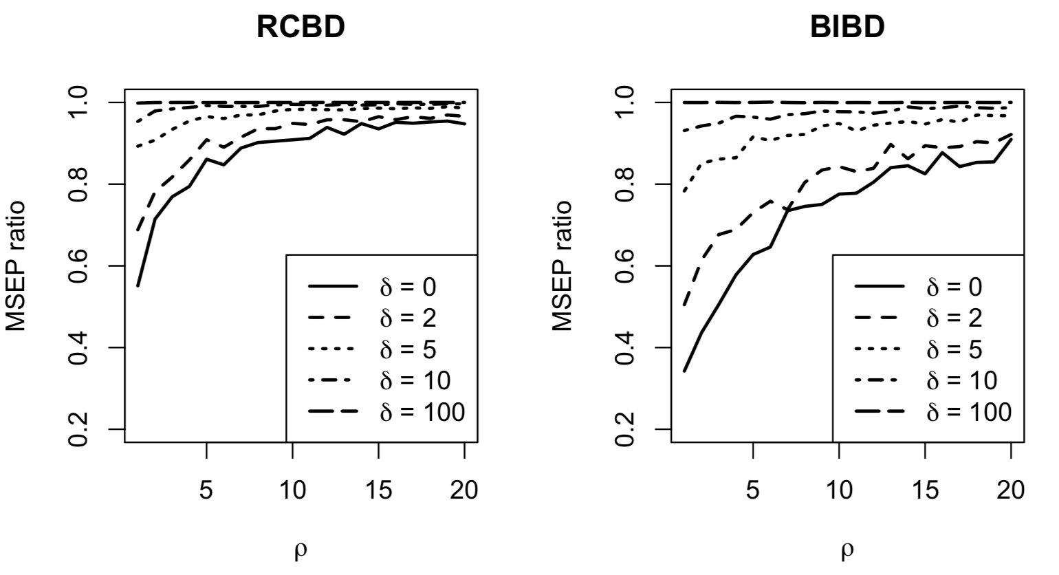
Figure 1: Empirical BLUP versus MLE mean squared error of prediction ratios for varying values of $\rho=\sigma_{b}^{2}/\sigma_{e}^{2}$, and ranges for treatment means.

The figure reveals that the EBLUP dominates the MLE with a smaller mean squared error in both RCBD and BIBD cases, but this advantage weakens as the ratio of block to error variance, $\rho$, increases. Also, with the same $\rho$ and treatment mean vector, $\delta$, the relative efficiency of the EBLUP compared to the MLE is higher for the BIBD than for RCBD.

4 Application

The English Premier League consists of 20 teams, three of which are relegated each year and replaced the next season by three teams from the English League Championship. During the course of a season each team plays every other team twice, once at home and once away. Here we attempt to use a mixed effects model and shrinkage estimation to predict the outcomes of remaining games based on each team’s performance in their first 7 home and away games. Since each team plays 19 home games the initial 7 home games for each team represent (approximately) 14 games per team in total, just over one third of a season. We use a model with the response being the difference, $y$, between the number of goals scored by the home team and the number scored by the away team because the difference between the number of goals scored by two teams is approximately normal. This follows from the fact, illustrated later in the Discussion, that the number of goals scored per game by each team is well approximated by a Poisson distribution, and the difference between two independent Poisson variables with means typical for the EPL is approximately normal.

The model for a particular game between (home) team $i$ and (away) team $j$ is

$$y_{ij}=\mu+h_{i}-a_{j}+e_{ij}\,,$$ (14)

where $h_{i}$ is a random effect representing the strength of team $i$ at home and $a_{j}$ is a random effect representing of the strength of team $j$ away. We assume that $h_{i}\sim\mbox{iid }N(0,\sigma^{2}_{h})$, $a_{j}\sim\mbox{iid }N(0,\sigma^{2}_{a})$, and $e_{ij}\sim\mbox{iid }N(0,\sigma^{2}_{e})$ for $i$ and $j$ in $\{1,2,\ldots,20\}$, but excluding cases in which $i=j$. The data used to train the model is unbalanced because different teams play different opponents in their first 7 home games.

Figure 3 shows the EBLUPs for the home and away effects for the 2017-18 season, where the teams are ordered by the sum of their predicted home and away effects. Thus, for example, Manchester United’s predicted home effect is 1.632, whereas West Ham United’s away effect is -1.216. If the end of season rankings of the 20 teams are predicted using this ordering, then the mean absolute error in predicted rankings is 3 for the 2017-18 season, and the correlation with the actual end of season ranking is 0.788. Figure 3 shows the actual and predicted end-of-season goal difference for each team in 2017-18. The predictions are computed by averaging over the 24 games that were not used to fit the home-and-away model (14) and combining this average with the known results for the 14 games that were used to fit the model. The actual goal differences based on the games used to fit the model and the end of season goal differences for each team are also plotted for comparison. The teams are sorted by the end of season goal differences.

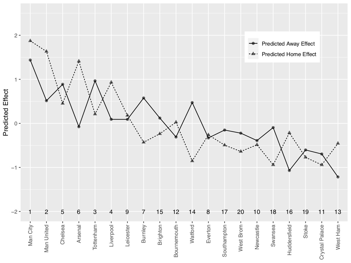
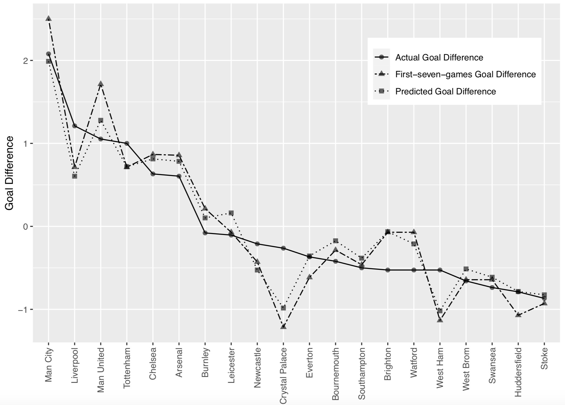
Figure 2: Empirical BLUPS for each team’s home and away effects for the 2017-18 season, and their actual end of season ranking.

Figure 3: Actual and predicted end-of-season goal difference, and actual first-seven-games goal difference for each team for the 2017-18 season.

In general we predict a win for the home team if the difference between the home and away effects are greater than a threshold, $d$, a loss if the difference is less than $-d$, and a tie if neither of these inequalities hold. Predicting ties is notoriously difficult in football. There is a long history of betting on the outcome of football games in Britain dating back to the 1920’s. The most famous ‘football pool’ involved picking a line of eight from the upcoming weekend’s games from all British professional leagues. One point was awarded for picking a home win, 1.5 points for an away win, 2 points for a 0-0 tie, and 3 points for a scoring tie. Millions of people took part in the pool each week resulting in a very large payout for the winners with the highest points total. The winners often had little knowledge of football and essentially picked their line at random. We used model (14) to pick ties, with $d=0.25$ for all the games (after the first 7 home games) in the 17 EPL seasons from 2001-2 to 2017-18, resulting in overall success rate of 0.290. The value $d=0.25$ was chosen based on a grid search, because this choice led to 1135 predicted draws which was the closest to the actual number, 1022.

The proportion of games that were ties during this period was 0.250, one-third of which were 0-0 ties. The complete results are given in Table 1. Based on this historical data the estimated win, loss and draw probabilities for the home team are 0.473, 0.277 and 0.250 respectively. Thus, if the result of a game is predicted at random, with 1/3 probability for each outcome, and factoring in the fact that one-third of draws are 0-0, the expected number of points using the scoring system described in the previous paragraphs is

$$(1)(0.473)/3+(1.5)(0.277)/3+(2)(0.25)/9+(3)(0.25)(2/9)=0.518\,.$$

Thus, the average score for a better who chooses a line of eight games at random is 4.144. In contrast, the model (14) correctly predicts wins, losses and draws with relative frequencies 0.322, 0.076 and 0.081 respectively. Also, among the correctly predicted draws one third were 0-0. Thus, the expected number of points based on predicting outcomes using the model (14) is $(1)(0.322)+(1.5)(0.076)+(2)(0.081)(1/3)+(3)(0.081)(2/3)=0.652$, or 5.216 for an eight game line. Although this is an improvement over random guessing, a score near the mean would never win the pool. Rather it is scores in the right tail of the distribution that determine the winner. By simulating lines of eight games using the multinomial distributions for the four outcomes (win, loss, no-score, and score-draw) one can establish that the model produces a score distribution that is stochastically larger than random guessing. So, using shrinkage estimation via a normal theory mixed model does improve the odds of winning, but we acknowledge that even doubling a random win probability on the order of $10^{-6}$, or even $10^{-7}$, would not be very helpful to a typical bettor.

Table 1: Actual versus predicted results for seasons 2001-2 to 2017-18 based on model (14). (D=draw, L=loss, W=win for the home team)

	Predicted.D	Predicted.L	Predicted.W	Actual Totals
Actual.D	329	162	531	1022
Actual.L	380	311	439	1130
Actual.W	426	187	1315	1928
Predicted Totals	1135	660	2285	4080

5 Use of Prior Information

Since there is data on EPL results from multiple seasons, it is natural to think about incorporating prior information about model parameters (specifically, the variance components) based on data from previous seasons. Consider the model (14) applied to a complete EPL season. If we ignore the fact teams do not play themselves, the design consists of two crossed (random) home and away team factors. The expected mean square (EMS) for the home team factor, after adjusting for the away team, is therefore approximately $19\sigma^{2}_{h}+\sigma^{2}_{e}$. Here we use a multiplier of 19 rather than 20 to account, at least approximately, for the fact that teams do not play themselves. Similarly, the EMS for the away team factor is approximately $19\sigma^{2}_{a}+\sigma^{2}_{e}$. It follows that the EMS estimates of the variance components have approximate marginal distributions given by $\widehat{\sigma}^{2}_{e}\sim\sigma^{2}_{e}\chi^{2}_{d_{e}}/d_{e}$, $\widehat{\sigma}^{2}_{h}\sim\sigma^{2}_{h}\chi^{2}_{d_{h}}/d_{h}$, and $\widehat{\sigma}^{2}_{a}\sim\sigma^{2}_{a}\chi^{2}_{d_{a}}/d_{a}$, where $d_{e}=20\times 19-19-19-1=341$, and $d_{h}$ and $d_{a}$ are obtained using Satterthwaite’s approximation (Satterthwaite, 1949).

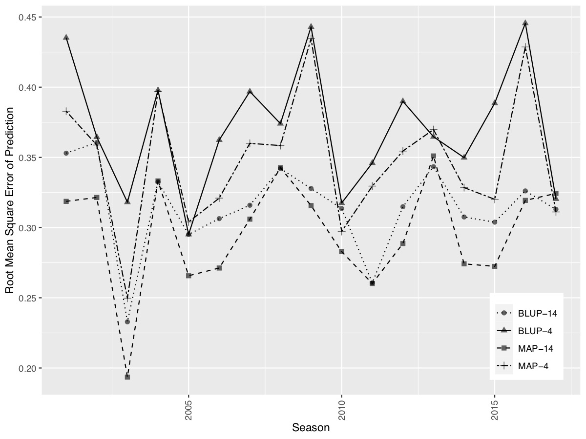
Figure 4: Comparison of RMSEP for BLUP and MAP predictors based on models (14) and (4) for seasons beginning in 2001 to 2017.

If $X\sim\sigma^{2}\chi^{2}/d$ and we assign an improper prior to $\sigma^{2}$ proportional to $1/\sigma^{2}$, then the posterior for $\sigma^{2}$ is inverse-Gamma with shape $\alpha=d/2$ and scale $\beta=dX/2$. It follows that an approximate maximum a posteriori (MAP) estimate of $\sigma^{2}$ under these modeling assumptions is the posterior mode, given by $\beta/(\alpha+1)=\frac{d/2}{d/2+1}X$. Figure 4 shows the RMSEP values for EBLUP and MAP predictors of goal differences for every game in each season after the models were trained on the first 7 home games for each team. The MAP predictors were computed using the blme package in R (R Core Team, 2021). There is noticable improvement using both home and away team factors (model 14) relative to only the home team factor (model 4). Also the inclusion of prior information about the variance components based on data from the previous season improves the predication accuracy in most years. This is reflected in the ability to predict the end of season rankings with the mean absolute deviations between actual and predicted rankings equal to 2.541, 2.735 for MAP and EBLUP respectively based on model (14), and 3.135 and 3.524 for MAP and EBLUP based on model (4), over the course of 17 seasons. The incorporation of prior information from the previous season also improve the prediction accuracy for ties to 0.298.

6 Discussion

Perhaps the most famous example of Stein shrinkage estimation concerns the prediction of baseball batting averages for 18 major league players based on their first 45 at bats during the 1970 season (Efron and Morris, 1975, 1977). In that setting the data consist of binomial counts with the individual hit probabilities being the quantities of interest. Since the variance of a binomial count depends on the success probability, the constant variance assumption in the classical James-Stein and James-Stein-Lindley estimators given in (1) and (2) is violated. Efron and Morris got around this issue using the variance stabilizing, arcsine square root transformation of the binomial proportions which results in transformed responses that are approximately normal with variances equal to 1. In the case of goal differences in football matches it is not clear that a transformation will help. For example, one might model the number of goals scored by the home and away teams separately using independent Poisson distributions, which would suggest the use of a square root transformation. In fact, the Poisson distribution does appear to be a good model for the number of goals scored by a particular team. For example, Figure 5 shows the relative frequency distribution of the number of goals scored in EPL home games by Manchester United from 2001 to 2018, and the corresponding probabilities for a Poisson distribution with the same mean, 2.14. Similar excellent fits of the Poisson distribution is found for most teams. However, the average number of goals scored per game is about 1 for bad teams and 2 for good teams. Over this range the square root transformation does not yield a good normal approximation, although it is close to being variance stabilizing. On the other hand, the difference of two independent Poisson variables with means in this range is well approximated by a normal. This fact is illustrated in Figure 6 where the exact distribution of the difference between two independent Poisson variables with means 2 and 1 is compared to a normal distribution with the same mean and variance. The normal approximation is even better for more evenly matched teams. Since different teams have different means the constant variance assumption underlying the JSL estimator is violated. However, with the means restricted to the range 1 to 2 the standard deviation of the difference only varies from $\sqrt{2}$ to 2. Of course the independence assumption is also questionable, as is the assumption that the team effects remain constant over the season. Thus, there is scope for improvements to the modeling approach described in this paper.

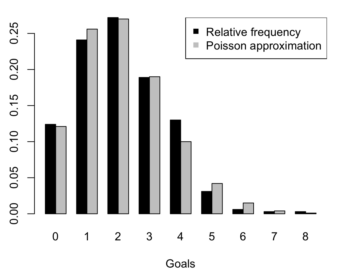
Figure 5: Distribution of Goals scored by Manchester United in home EPL games between 2001 and 2018 and Poisson approximation.

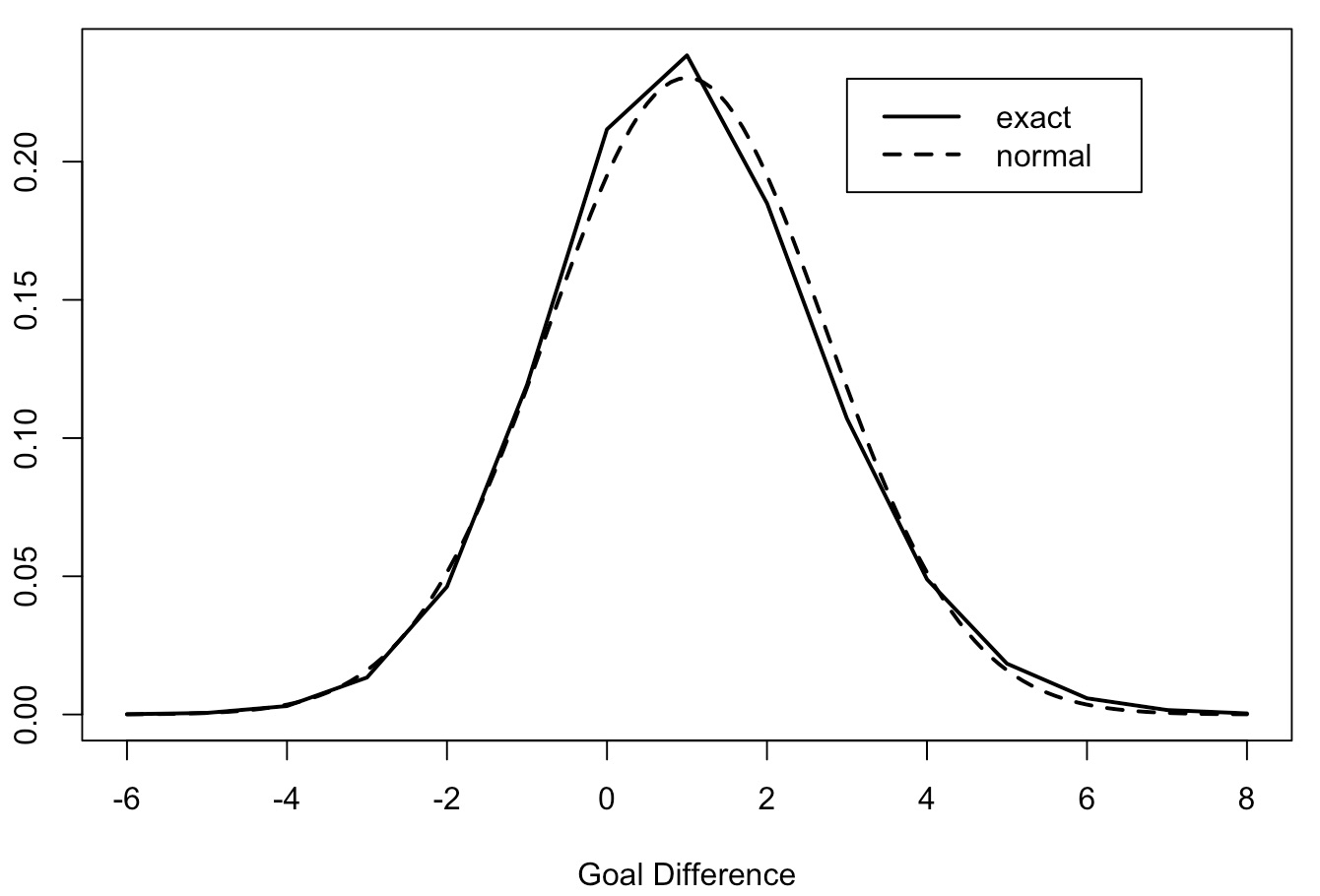
Figure 6: Normal approximation to the exact distribution of the difference between two independent Poisson variables with means 2 and 1 respectively.

7 Appendix

Proof of Theorem: Suppose ${\mathbf{y}}\sim N({\mbox{\boldmath$\mu$}}_{y},a{\mathbf{I}}_{t}+b{\mathbf{J}}_{t})$, where $a>0$ and $b>0$. Let ${\mathbf{V}}=a{\mathbf{I}}_{t}+b{\mathbf{J}}_{t}$ and note that ${\mathbf{V}}={\mathbf{H}}{\mathbf{D}}{\mathbf{H}}^{T}$ where ${\mathbf{H}}$ is the $t\times t$ Helmert matrix and ${\mathbf{D}}=\mbox{diag}(a+tb,a{\mbox{\boldmath$1$}}_{t-1}^{T})$. Define ${\mathbf{x}}={\mathbf{V}}^{-1/2}{\mathbf{y}}$, so that ${\mathbf{x}}\sim N({\mbox{\boldmath$\mu$}}_{x}={\mathbf{V}}^{-1/2}{\mbox{\boldmath$\mu$}}_{y},{\mathbf{I}}_{t})$. It follows that the JSL estimator for ${\mbox{\boldmath$\mu$}}_{x}$, given by

$$\widehat{{\mbox{\boldmath$\mu$}}}_{x}^{JSL}={\mbox{\boldmath$1$}}_{t}\bar{x}+\left(1-\frac{1}{S_{x}/(t-3)}\right)({\mathbf{x}}-{\mbox{\boldmath$1$}}_{t}\bar{x})\,,$$

where $\bar{x}={\mbox{\boldmath$1$}}_{t}^{T}{\mathbf{x}}/t$ and $S_{x}=||{\mathbf{x}}-{\mbox{\boldmath$1$}}_{t}\bar{x}||^{2}$, has the property that

$$E_{{\mbox{\boldmath$\mu$}}_{x}}(||\widehat{{\mbox{\boldmath$\mu$}}}_{x}-{\mbox{\boldmath$\mu$}}_{x}||^{2})\leq E_{{\mbox{\boldmath$\mu$}}_{x}}(||{\mathbf{x}}-{\mbox{\boldmath$\mu$}}_{x}||^{2})$$ (15)

for all ${\mbox{\boldmath$\mu$}}_{x}$.

Now, the spectral decomposition of ${\mathbf{V}}$ implies that ${\mathbf{V}}^{1/2}{\mbox{\boldmath$1$}}_{t}\bar{x}={\mbox{\boldmath$1$}}_{t}\bar{y}$. Furthermore,

$${\mathbf{V}}^{-1}=\frac{1}{a}\left({\mathbf{I}}_{t}-\frac{b}{a+tb}{\mathbf{J}}_{t}\right)$$ (16)

and ${\mathbf{J}}_{t}({\mathbf{y}}-{\mbox{\boldmath$1$}}_{t}\bar{y})={\mbox{\boldmath$0$}}$, together imply that $S_{x}=S_{y}/a$ and hence that

$$V^{1/2}\widehat{{\mbox{\boldmath$\mu$}}}_{x}^{JSL}={\mbox{\boldmath$1$}}_{t}\bar{y}+\left(1-\frac{a}{S_{y}/(t-3)}\right)({\mathbf{y}}-{\mbox{\boldmath$1$}}_{t}\bar{y})=\widehat{{\mbox{\boldmath$\mu$}}}_{y}\,.$$

It follows from (15) that

$$E_{{\mbox{\boldmath$\mu$}}_{y}}\left\{(\widehat{{\mbox{\boldmath$\mu$}}}_{y}-{\mbox{\boldmath$\mu$}}_{y})^{T}{\mathbf{V}}^{-1}(\widehat{{\mbox{\boldmath$\mu$}}}_{y}-{\mbox{\boldmath$\mu$}}_{y})\right\}\leq E_{{\mbox{\boldmath$\mu$}}_{y}}\left\{({\mathbf{y}}-{\mbox{\boldmath$\mu$}}_{y})^{T}{\mathbf{V}}^{-1}({\mathbf{y}}-{\mbox{\boldmath$\mu$}}_{y})\right\}$$

The result now follows by noting that (16) implies

$$a({\mathbf{y}}-{\mbox{\boldmath$\mu$}}_{y})^{T}{\mathbf{V}}^{-1}({\mathbf{y}}-{\mbox{\boldmath$\mu$}}_{y})=||{\mathbf{y}}-{\mbox{\boldmath$\mu$}}_{y}||^{2}+\frac{tb}{a+tb}(\bar{y}-\bar{\mu}_{y})^{2}\,,$$

where $\bar{\mu}_{y}={\mbox{\boldmath$1$}}_{t}^{T}{\mbox{\boldmath$\mu$}}_{y}/t$, and

$$a(\widehat{{\mbox{\boldmath$\mu$}}}_{y}-{\mbox{\boldmath$\mu$}}_{y})^{T}{\mathbf{V}}^{-1}(\widehat{{\mbox{\boldmath$\mu$}}}_{y}-{\mbox{\boldmath$\mu$}}_{y})=||\widehat{{\mbox{\boldmath$\mu$}}}_{y}-{\mbox{\boldmath$\mu$}}_{y}||^{2}+\frac{tb}{a+tb}(\bar{\widehat{\mu}}_{y}-\bar{\mu}_{y})^{2}\,,$$

where $\bar{\widehat{\mu}}_{y}={\mbox{\boldmath$1$}}_{t}^{T}\widehat{{\mbox{\boldmath$\mu$}}}_{y}/t=\bar{y}$.

References

- Cochran and Cox (1957) Cochran, W. and Cox, G. (1957). Experimental Designs. John Wiley & Sons, 2 edition.
- Efron and Morris (1973) Efron, B. and Morris, C. (1973). Stein’s estimation rule and its competitor – an empirical bayes approach. Journal of the American Statistical Association, 68, 117–130.
- Efron and Morris (1975) Efron, B. and Morris, C. (1975). Data analysis using stein’s estimator and it’s generalizations. Journal of the American Statistical Association, 70(350), 311–319.
- Efron and Morris (1977) Efron, B. and Morris, C. (1977). Stein’s paradox in statistics. Scientific American, 236(5), 119–127.
- James and Stein (1961) James, W. and Stein, C. (1961). Estimation with quadratic loss. Proc. 4th Berkeley Sympos. on Math. Statist. and Prob., pages 361–379.
- Lehmann and Casella (1998) Lehmann, E. L. and Casella, G. (1998). Theory of Point Estimation. Springer, 2 edition.
- Moser (1996) Moser, B. (1996). Linear Models: A Mean Model Approach. Academic Press.
- R Core Team (2021) R Core Team (2021). R: A Language and Environment for Statistical Computing. R Foundation for Statistical Computing, Vienna, Austria.
- Satterthwaite (1949) Satterthwaite, F. (1949). An approximate distribution of estimates of variance components. Biometrics Bulletin, 2(6), 110–114.
- Stein (1955) Stein, C. (1955). Inadmissibility of the usual estimator for the mean of the multivariate normal distribution. Proc. 3th Berkeley Sympos. on Math. Statist. and Prob., pages 197–206.