A pithy look at the Polytope Algebra

Abstract.

This is a hands on introduction to McMullen’s Polytope Algebra. More than interesting on its own, this algebra was McMullen’s tool to give a combinatorial proof of the g-theorem.

1. Introduction

One of the biggest achievements in polytope theory was the complete characterization of $f$-vectors of simplicial polytopes, known as the $g$-theorem (for a precise statement see [12, Chapter 3]). In the early 70’s Peter McMullen conjectured a set of necessary and sufficient conditions and less than a decade later Lou Billera and Carl Lee proved sufficiency, whereas Richard Stanley proved necessity. For an interesting survey about the history of this result we refer the reader to [3].

Stanley’s proof in [13] imports a result from complex geometry, namely the Hard-Lefschetz theorem, so for a while people attempted to find a more combinatorial proof, one that used more elementary arguments. McMullen succeeded initially in [10] and then corrected and simplified parts of it in [11]. The heart of the $g$-theorem lies in associating, to each simplicial polytope $P$, a finite dimensional algebra with particular properties. By now there are many different ways of doing this. For instance, in [2] Billera uses piecewise polynomial functions on a fan (an approach also explored by Brion [4]), and in [5] Fulton-Sturmfels use the Chow ring of the associated toric variety which they show is isomorphic to the Minkowski weights, which is the same ring that McMullen employs in [11] although he constructs it from his earlier work in [9].

Here we give an overview of the Polytope Algebra as developed in [9]. Of all the approaches mentioned above, this one is of the easiest to define and in a way the most “polytopal”. Apart from the intrinsic interest, we also wanted to introduce, in a natural way, the notion of Minkowski weights which continues to play an important role in research nowadays, for example in tropical geometry [8].

2. Polytopes and their faces

Definition 2.1.

A polytope $P\subset\mathbb{R}^{d}$ is the convex hull of finitely many points $\{\textbf{v}_{1}.\cdots,\textbf{v}_{m}\}$. More precisely,

$$P=\textrm{conv}\{\textbf{v}_{1},\cdots,\textbf{v}_{m}\}=\left\{\sum_{i=1}^{m}\lambda_{i}\textbf{v}_{i}:\lambda_{1}+\cdots+\lambda_{m}=1,\lambda_{1},\cdots,\lambda_{m}\geq 0\right\}.$$

An inclusion minimal set of points whose convex hull is $P$ is called the vertex set of $P$, $\textrm{vert}(P)$. Such a minimal set exists and is unique.

Theorem 2.2 (Minkowski-Weyl).

Every polytope $P$ is the bounded intersection of finitely many halfspaces. More precisely, there exist $\textbf{a}_{1},\cdots,\textbf{a}_{n}\in\mathbb{R}^{d}\backslash\{0\}$ and $b_{1},\cdots,b_{n}\in\mathbb{R}$ such that

$$P=\left\{\textbf{x}\in\mathbb{R}^{d}:\textbf{a}_{1}^{t}\textbf{x}\leq b_{1},\cdots,\textbf{a}_{n}^{t}\textbf{x}\leq b_{n}\right\}.$$

As before, there may be redundant inequalities. An inclusion minimal set of inequalities that define $P$ is called the set of facet inequalities. Such a minimal set exists and is unique.

Definition 2.3.

Let $P\subset\mathbb{R}^{d}$ be a polytope. We define the following notions.

1. The affine hull of $P$: $\textrm{aff}(P)=\bigcap\left\{L\subset\mathbb{R}^{d}\textrm{ affine space such that }P\subset L\right\}$.

2. The linear span of $P$: $\textrm{lin}(P)=$ the linear subspace that is parallel to $\textrm{aff}(P)$.

3. The relative interior of $P$: $\textrm{relint}(P)=$ the interior of $P$ relative to $\textrm{aff}(P)$.

4. The dimension of $P$: $\dim(P)=\dim\textrm{lin}(P)$.

Basic information: From now on we are going to repeatedly use the following notation. $P$ is a $d$-dimensional polytope, or $d$-polytope, with $n$ facet inequalities (or just facets for short) and $m$ vertices. The set of all polytopes in $\mathbb{R}^{d}$ (not necessarily full dimensional) is denoted ${\mathcal{P}}_{d}$ and $\hat{{\mathcal{P}}_{d}}:={\mathcal{P}}_{d}\backslash\{\emptyset\}$.

2.1. Faces of polytopes.

For any $\textbf{c}\in\mathbb{R}^{d}$ (which we will think of as a linear functional) define

$$P^{\textbf{c}}: =\{\textbf{x}\in P:\textbf{c}^{t}\textbf{x}\geq\textbf{c}^{t}\textbf{y},\forall\textbf{y}\in P\},$$

$$=\{\textbf{x}\in P:\textbf{c}^{t}\textbf{x}=\delta\},\quad\delta=\underset{\textbf{x}\in P}{\max}\hskip 5.0pt\textbf{c}^{t}\textbf{x}.$$

Subsets of $P$ of the above form are called faces of $P$. If $P=\textrm{conv}\{\textbf{v}_{1},\cdots,\textbf{v}_{m}\}$ is the vertex description of $P$, then $P^{\textbf{c}}=\textrm{conv}\{\textbf{v}_{i}:\textbf{c}^{t}v_{i}=\delta\}$, so faces are polytopes themselves. Moreover, there can be only finitely many faces. By convention, $\emptyset$ and $P$ itself are faces.

Remark 2.4.

In what follows we will only consider face directions c such that $|\textbf{c}|=1$.

Definition 2.5.

Let $P$ be a polytope and let $\mathcal{F}_{k}(P)$ be the set of $k$-dimensional faces. Without a subscript $\mathcal{F}(P)$ is the set of all faces of $P$. Equipped with the partial order given by containment, $\mathcal{F}(P)$ is called the face lattice of $P$. This captures the combinatorial information of $P$. Two polytopes are said to be combinatorially equivalent if they have isomorphic face lattices.

Definition 2.6.

A weaker invariant is the f-vector: $f(P)=(f_{0},f_{1},\cdots,f_{d-1},f_{d})$. Where $f_{i}$ is the number of $i$-dimensional faces of $P$ (recall that faces are themselves polytopes, hence they have dimension). Often people add $f_{-1}=1$ for the empty set. Also note that $f_{d}=1$ always. The 0-faces are the vertices, 1-faces the edges, and $(d-1)$-faces are the facets.

We say a $d$-polytope is simple if each vertex is contained in exactly $d$ facets.

3. Valuations.

For any set $S\subset\mathbb{R}^{d}$ denote by $[S]$ the indicator function from $\mathbb{R}^{d}$ to $\{0,1\}$ defined as

$$[S](p)=\begin{cases}1,\quad p\in S,\\ 0,\quad p\notin S.\end{cases}$$

Definition 3.1.

A function $f:\mathbb{R}^{d}\longrightarrow\mathbb{Z}$ is a polytopal simple function if it can be written as

$$f=\alpha_{1}[Q_{1}]+\cdots+\alpha_{k}[Q_{k}],\quad\alpha_{i}\in\mathbb{Z},$$

with $Q_{1},\cdots,Q_{k}$ polytopes.

Notation 3.2.

Recall that ${\mathcal{P}}_{d}=\{\textrm{ polytopes }\subset\mathbb{R}^{d}\}$ and now we define $\mathcal{SP}_{d}:=\{\textrm{ polytopal simple functions }\}$. Often we won’t distinguish between a polytope and its indicator function.

By definition, indicator functions of ${\mathcal{P}}_{d}$ span $\mathcal{SP}_{d}$ but they are far from a basis, they satisfy relations like $[P\cup Q]=[P]+[Q]-[P\cap Q]$.

Definition 3.3.

A valuation is any group homomorphism $\phi:\mathcal{SP}_{d}\longrightarrow G$ with $G$ an abelian group.

The first and most fundamental valuation is the Euler characteristic (See [1, Theorem 2.4]).

Theorem 3.4.

There exists a unique valuation $\chi:{\mathcal{P}}_{d}\longrightarrow\mathbb{Z}$, called the Euler characteristic with

• $\chi(\emptyset)=0$.

• $\chi(P)=\begin{cases}1,\quad P\in\hat{{\mathcal{P}}_{d}}\\ 0,\quad\textrm{else.}\end{cases}$

Even though $\mathcal{SP}_{d}$ is spanned by indicator functions of polytopes, it also contains indicator functions of other non polytopal sets. For instance, the Euler formula is equivalent to the relation

Lemma 3.5.

Let $P$ be a $d$-polytope then

$$[P^{\circ}]=\sum_{F\subseteq P}(-1)^{\textrm{dim}(P)-\textrm{dim}(F)}[F].$$

Furthermore $\chi\left([P^{\circ}]\right)=(-1)^{\textrm{dim}(P)}$.

Indicators functions come with a natural product, namely pointwise multiplication, but we consider a different product that gives the following ring structure.

Proposition 3.6.

The map $\ast:\mathcal{SP}_{d}\times\mathcal{SP}_{d}\to\mathcal{SP}_{d}$ defined by $[P]\ast[Q]:=[P+Q]$ gives $\mathcal{SP}_{d}$ the structure of a commutative ring. The multiplicative unit is $[\textbf{0}]$, the indicator function at the origin.

With this operation we gain some interesting inverses.

Proposition 3.7.

Let $P\in\hat{{\mathcal{P}}_{d}}$, then $[P]$ is invertible:

(3.1) $$[P]^{-1}=(-1)^{\dim P}[-\textrm{relint}(P)].$$

The next proposition is fundamental for what follows.

Proposition 3.8.

If $P=\textrm{conv}\{v_{1},\cdots,v_{m}\}$ is a polytope, then

(3.2) $$\left([P]-[v_{1}]\right)*\left([P]-[v_{2}]\right)*\cdots*\left([P]-[v_{m}]\right)=0.$$

Let’s first illustrate an example.

Example 3.9.

Let $P$ be a one dimensional polytope $[a,b]\subset\mathbb{R}$. Then $([P]-[a])*([P]-[b])=[2P]-[P+a]-[P+b]+[a+b]=0$, as can be seen by inspection in Figure 1.

Figure 1. An illustration of Proposition 3.8

Sketch of proof.

We first prove it for $P=\Delta_{m-1}=\textrm{conv}\{\mathbf{e}_{1},\cdots,\mathbf{e}_{m}\}=\{\textbf{x}\in\mathbb{R}^{m}:x_{i}\geq 0,\quad\sum x_{i}=1\}.$ We define $\mathbf{e}_{I}:=\sum_{i\in I}\mathbf{e}_{i}$ for $I\subset[m]$. We must show that

(3.3) $$\sum_{I\subset[m]}(-1)^{|I|}\left[(m-|I|)\Delta_{m-1}+\mathbf{e}_{I}\right]=0.$$

For $q\in\mathbb{R}^{m}$ how do we decide if $q\in\left[(m-|I|)\Delta_{m-1}+\mathbf{e}_{I}\right]$? This is equivalent to $q-\mathbf{e}_{I}\in(m-|I|)\Delta_{m-1}$. This happens if and only if

$$q-\mathbf{e}_{I}\geq 0\qquad\sum q_{i}=m,$$

where the first inequality is coordinate wise. Now define $I_{0}:=\{i:q_{i}\geq 1\}$. For a fixed $q$ with $\sum q_{i}=m$ the value of the function in the left hand side of Equation (3.3) is

$$\sum_{I\subset I_{0}}(-1)^{|I|}=\sum_{j=0}^{|I_{0}|}\binom{I_{0}}{j}(-1)^{j}=(1-1)^{|I_{0}|}=\begin{cases}0,\quad I_{0}\neq\emptyset,\\ 1,\quad I_{0}=\emptyset,\end{cases}$$

but $I_{0}$ will never be empty since we are asumming $\sum q_{i}=m$. This finishes the proof for the standard simplex.

For the general case we can write $P=\pi(\Delta_{m-1})$, where $\pi:\mathbb{R}^{m}\longrightarrow\mathbb{R}^{d}$, defined by mapping $\mathbf{e}_{i}\longrightarrow v_{i}$. Then one can argue that $\pi$ induces a map $\pi_{*}:\mathcal{SP}_{m}\to\mathcal{SP}_{d}$ sending $\pi_{*}[P]=[\pi(P)]$ for $P\in{\mathcal{P}}_{m}$ and such that the linear relations are preserved. ∎

4. The Polytope Algebra

We define $\mathcal{T}:=\mathbb{Z}\{[P+t]-[P]\quad\forall P\in{\mathcal{P}}_{d},t\in\mathbb{R}^{d}\}.$ This is actually an ideal of $\mathcal{SP}_{d}$, called the translation ideal.

Definition 4.1.

The polytope algebra is defined as

$$\Pi^{d}:=\mathcal{SP}_{d}/\mathcal{T}.$$

We denote by $\llbracket P\rrbracket$ the class of $[P]$ in $\Pi^{d}$.

The multiplicative identity is $1:=\llbracket\{\textbf{0}\}\rrbracket$, the class of the origin as a zero dimensional polytope.

Definition 4.2.

We define also dilation maps which are in fact endormorphism. Let $D_{\lambda}:\Pi^{d}\to\Pi^{d}$ be defined in the generators as $D_{\lambda}\llbracket P\rrbracket:=\llbracket\lambda P\rrbracket$ for $\lambda\in\mathbb{R}_{\geq 0}$. Notice that $D_{\lambda}$ and $D_{\lambda^{-1}}$ are inverses to each other for $\lambda>0$.

Example 4.3.

Let’s begin by understanding $\Pi^{1}$. This is generated by integer combinations of segments. For each line segment $[a,b]$ we have $\llbracket[a,b]\rrbracket=\llbracket[a,b)\rrbracket+\llbracket\{b\}\rrbracket=\llbracket[0,b-a)\rrbracket+\llbracket\{0\}\rrbracket$, since we can decompose and translate the pieces. Notice that the sum of two classes of half open segments can be represented again by a half open segment; $\llbracket[0,r)\rrbracket+\llbracket[0,s)\rrbracket=\llbracket[0,r)\rrbracket+\llbracket[r,s+r)\rrbracket=\llbracket[0,s+r)\rrbracket$.

It is not true that $\llbracket[0,s)\rrbracket\ast\llbracket[0,r)\rrbracket=\llbracket[0,s+r)\rrbracket$, since the definition of the product with Minkowski sums only is intended for the generators, the indicator functions of polytopes. Indeed we have

$$\llbracket[0,s)\rrbracket\ast\llbracket[0,r)\rrbracket=\left(\llbracket[0,s]\rrbracket-\llbracket\{0\}\rrbracket\right)\ast\left(\llbracket[0,r]\rrbracket-\llbracket\{0\}\rrbracket\right),$$

which we already saw in Example 3.9 to be zero.

With this is mind, $\Pi^{1}\cong\mathbb{Z}\oplus\mathbb{R}$ with multiplication defined by $(a,b)\cdot(a^{\prime},b^{\prime})=(aa^{\prime},ab^{\prime}+a^{\prime}b)$.

Now that we understand $\Pi^{1}$, we move on to the general case. The following is the main structural result.

Theorem 4.4.

The polytope algebra is a graded ring, generated in degree 1. $\Pi^{d}=\Pi_{0}\oplus\Pi_{1}\oplus\cdots\oplus\Pi_{d}$. Furthermore

• $\Pi_{0}\cong\mathbb{Z}$.

• $\Pi_{i}$ is an $\mathbb{R}$-vector space for $i>0$.

• $\Pi_{d}\cong\mathbb{R}$.

The theorem means that $\Pi^{d}$ is almost an $\mathbb{R}$-algebra, except for the fact that $\Pi_{0}\cong\mathbb{Z}$. Notice that $\Pi^{d}$ comes from $\mathcal{SP}_{d}$ which is made of integer combinations of indicator functions, so the fact that we end up with a $\mathbb{R}$ action should be surprising, in fact we will see below that scaling can be complicated. As a first step in proving Theorem 4.4 we have the following proposition.

Proposition 4.5.

The map $\Pi^{d}\longrightarrow\mathbb{Z}$ induced by $\chi$ allows us to decompose $\Pi^{d}=\mathbb{Z}\oplus\Pi_{+}$ as a direct sum, where $\Pi_{+}:=\textrm{ker }\chi$.

Proof.

Decompose $x=\sum\alpha_{i}\llbracket P_{i}\rrbracket\in\Pi^{d}$ as

(4.1) $$x=\sum\alpha_{i}\chi(P_{i})\cdot 1+\sum\alpha_{i}\left(\llbracket P_{i}\rrbracket-1\right)=\chi(x)\cdot 1+\left(x-\chi(x)\cdot 1\right).$$

∎

From Equation 4.1 we have that $\Pi_{+}=\mathbb{Z}\{\llbracket P\rrbracket-1:\quad P\in\hat{{\mathcal{P}}}_{d}\}$. Proposition 3.8 in the polytope algebra means that all those generators are nilpotent. More precisely:

Corollary 4.6.

For $P\in\hat{{\mathcal{P}}}_{d}$ we have $\Big{(}\llbracket P\rrbracket-1\Big{)}^{r}=0$ in $\Pi^{d}$ for $r>d$.

Proof.

From Theorem 3.8 we know that $\Big{(}\llbracket P\rrbracket-1\Big{)}^{f_{0}(P)}=0$. Now we argue that we can lower the exponent. Notice that $\llbracket nP\rrbracket=\llbracket P+P\cdots+P\rrbracket=\llbracket P\rrbracket^{n}$ so we can write

(4.2) $$\llbracket nP\rrbracket=\left(1+\left(\llbracket P\rrbracket-1\right)\right)^{n}=\sum_{k=0}^{n}\binom{n}{k}\left(\llbracket P\rrbracket-1\right)^{k}.$$

Every polytope can be triangulated which means we can always write, through inclusion-exclusion, $\llbracket P\rrbracket=\sum\alpha_{i}\llbracket T_{i}\rrbracket$, where each $T_{i}$ is a simplex of dimension $\leq d$ (and hence with at most $d+1$ vertices) and $\alpha_{i}\in\{-1,+1\}$. When dilating $P$ we can dilate each piece so that

(4.3) $$\llbracket nP\rrbracket=\sum\alpha_{i}\llbracket nT_{i}\rrbracket.$$

Expanding the right hand side with an analogous relation to Equation 4.2 for each $T_{i}$, we get a polynomial in $n$ with coefficients in $\Pi^{d}$ of degree at most $d$, since all terms $\left(\llbracket T_{i}\rrbracket-1\right)^{r}$ vanish for $r>d$. This means that the right hand side of Equation 4.2 is also a polynomial in $n$ of degree $\leq d$ and hence $\left(\llbracket P\rrbracket-1\right)^{r}$ vanish for $r>d$. ∎

Theorem 4.7.

The abelian group $\Pi_{+}$ is a $\mathbb{Q}$-vector space.

This is a nontrivial statement. We need to make sense of $\frac{1}{m}x$ for $x\in\Pi_{+}$, more precisely, we need that for every $m\in\mathbb{Z}_{>0}$ there exists a unique $h\in\Pi_{+}$ with $x=m\cdot h$. We prove existence and uniqueness in two separate lemmas. Together they prove Theorem 4.7.

Lemma 4.8.

The abelian group $\Pi_{+}$ is divisible. For every $x\in\Pi_{+}$ and $m\in\mathbb{Z}_{>0}$, there exist $h\in\Pi_{+}$ such that $m\cdot h=f$.

Remark 4.9.

It is important to keep in mind that if $P$ is a polytope, then $2\llbracket P\rrbracket$ is not equal to $\llbracket 2P\rrbracket$, the indicator of the second dilation of $P$. One quick way to remember this is to apply Euler characteristic: $\chi\left(2\llbracket P\rrbracket\right)=2$ whereas $\chi\left(\llbracket 2P\rrbracket\right)=1$.

Proof.

The following proof is indirect and dry. To see how to actually divide see Example 4.11. It is enough to show the result for $m>1$ prime. Consider $N=m^{e}>d+1$ a large power of $m$. Then we have

$$\llbracket P\rrbracket-1=\llbracket\frac{1}{N}P\rrbracket^{N}-1=\sum_{i=1}^{d}\binom{N}{i}\left(\llbracket\frac{1}{N}P\rrbracket-1\right)^{i}.$$

Now since $m$ is prime and $N$ is a power of $m$, we have that $m$ divides all the binomial coefficients. ∎

Example 4.10.

Notice that in the real line it is straighforward to divide half open segments, since $m\cdot[0,r/m)=[0,r)$ up to translation.

Example 4.11.

Now sketch an example in two dimensions. Again we will not divide a whole polytope, but a polytope minus a point. Since all points are equivalent under translation, we choose to remove a vertex.

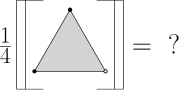
Figure 2. We need to find an integer combination of polytopes $h$ such that $\llbracket P\rrbracket=4h$

The idea now is that we are going to decompose that simplex in a convenient way. Along the way we will get 4 copies of its $\frac{1}{4}$-dilation, as may be expected, but we also get a number of products of simplices of strictly smaller dimensions. Then by induction in dimension we can divide each of them. See Figure 3.

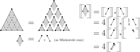
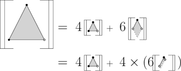
Figure 3. An example of division by 4.

Lemma 4.12.

The abelian group $\Pi_{+}$ has no torsion elements.

Proof.

Consider the following filtration $\Pi_{+}=Z_{1}\supset Z_{2}\supset\cdots\supset Z_{d}\supset Z_{d+1}$ where $Z_{r}$ is generated by elements of the form $\left(\llbracket P\rrbracket-1\right)^{j}$ for $j\geq r$. The proof of the lemma follows from two observations.

The first one is that $D_{\lambda}\left(\llbracket P\rrbracket-1\right)^{r}=\left(\llbracket\lambda P\rrbracket-1\right)^{r}$, since $D_{\lambda}$ is a ring endomorphism, so it commutes with taking powers. This implies that $D_{\lambda}Z_{r}\subset Z_{r}$ and $Z_{r}\subset D_{\lambda^{-1}}Z_{r}$.

The second observation is that if $x\in Z_{r}$, then

(4.4) $$D_{n}x-n^{r}x\in Z_{r+1},$$

for $n$ a natural number. It is enough to check it on the generators. We apply Equation 4.2

(4.5) $$D_{n}\left(\llbracket P\rrbracket-1\right)=\left(\llbracket nP\rrbracket-1\right)=\binom{n}{1}\left(\llbracket P\rrbracket-1\right)+\binom{n}{2}\left(\llbracket P\rrbracket-1\right)^{2}+\cdots.$$

Raising the above expression to the $r$ power we get that $D_{n}\left(\llbracket P\rrbracket-1\right)^{r}-n^{r}\left(\llbracket P\rrbracket-1\right)^{r}\in Z_{r+1}$. Since it is true for the generators then Equation 4.4 holds for all $Z_{r}$.

Now we finish the proof of the lemma. Let $x\in Z_{r}$ for some $r\geq 1$, and $nx=0$ for a natural $n$. Then $D_{n}x=D_{n}x-n^{r}x$ since $nx=0$ and hence $D_{n}x\in Z_{r+1}$ by 4.4 and also $x\in D_{n^{-1}}Z_{r+1}\subset Z_{r+1}$. This implies that $x\in Z_{j}$ for $j>>0$, but since they are eventually zero, $x$ must be zero.

∎

Combining Lemmas 4.12 and 4.8, we get Theorem 4.7. Now that we can make sense of rational multiples of element in $z\in\Pi_{+}$, we can define the exponential and the logarithm as formal power series with coefficients in $\mathbb{Q}$.

$$\exp(z):=\sum_{k\geq 0}\frac{1}{k!}z^{k},\qquad\log(1+z)=\sum_{k\geq 1}\frac{(-1)^{k-1}}{k}z^{k}.$$

The usual identities formally apply

$$\log\exp(z)=\exp\log(z)=z,$$

$$\exp(a+b)=\exp(a)\cdot\exp(b),$$

$$\log(a\cdot b)=\log(a)+\log(b).$$

With this in mind, we can define

$$\log(\llbracket P\rrbracket)=\log(1+\left(\llbracket P\rrbracket-1\right))=\sum_{k\geq 1}^{d}\frac{(-1)^{k-1}}{k}\left(\llbracket P\rrbracket-1\right)^{k},$$

which is a finite sum since $\left(\llbracket P\rrbracket-1\right)^{i}=0,i>d$.

Theorem 4.13.

For $P\in{\mathcal{P}}_{d}$, define $p:=\log\left(\llbracket P\rrbracket\right)$, then

(4.6) $$\llbracket P\rrbracket^{n}=\llbracket nP\rrbracket=1+pn+\frac{1}{2}p^{2}n^{2}+\cdots+\frac{1}{d!}p^{d}n^{d}.$$

Proof.

We simply manipulate our expressions:

(4.7) $$\llbracket nP\rrbracket=\llbracket P\rrbracket^{n}=\exp\left(\log\llbracket P\rrbracket^{n}\right)=\exp\left(np\right)=\sum_{i=0}^{d}\frac{1}{i!}p^{i}n^{i}$$

∎

A consequence of Theorem 4.13 is that for $n=1$:

(4.8) $$\llbracket P\rrbracket=1+p+\frac{1}{2}p^{2}+\cdots+\frac{1}{d!}p^{d}.$$

which is going to be our graded decomposition.

Definition 4.14.

Define $\Pi_{k}:=\mathbb{Z}\{\frac{1}{k!}\log\left(\llbracket P\rrbracket\right)^{k}\quad P\in{\mathcal{P}}_{d}\}$.

With this we now have $\Pi=\Pi_{0}+\Pi_{1}+\cdots+\Pi_{d}$. However we want this sum to be direct. For this we shall use our dilation maps. We have:

$$D_{r}(\log\llbracket P\rrbracket)=\log D_{r}(\llbracket P\rrbracket)=\log(\llbracket rP\rrbracket)=\log(\llbracket P\rrbracket^{r})=r\log(\llbracket P\rrbracket).$$

Moreover we have

$$x\in\Pi_{k}\Longleftrightarrow D_{r}x=r^{k}x\quad r\in\mathbb{Q}_{>0}.$$

Proposition 4.15.

We have $\Pi=\Pi_{0}\oplus\Pi_{1}\oplus\cdots\oplus\Pi_{d}$ as a direct sum.

Proof.

Suppose there exist $x_{i}\in\Pi_{i}$ with $x_{0}+x_{1}+\cdots+x_{d}=0$. From this, we conclude $D_{N}(x_{0}+x_{1}+\cdots+x_{d})=0$ which is the same as $x_{0}+x_{1}N^{1}+x_{2}N^{2}+\cdots x_{d}N^{d}=0$. This last equality is true for all $N>0$ hence we can conclude that $x_{i}=0.$ ∎

Proposition 4.16.

The decomposition $\Pi=\Pi_{0}\oplus\Pi_{1}\oplus\cdots\oplus\Pi_{d}$ gives a standard grading.

Proof.

What we need to prove is that $x\in\Pi_{i},y\in\Pi_{j}$ imply $x\ast y\in\Pi_{i+j}$. This follows from the fact that $D_{r}$ is a ring map,

$$D_{r}(x\ast y)=D_{r}(x)\ast D_{r}(y)=r^{i}x\ast r^{j}y=r^{i+j}(x\ast y).$$

∎

Corollary 4.17.

For any $\phi:{\mathcal{P}}_{d}\longrightarrow G$ translation invariant valuation, $\phi$ is homogeneous of degree $k$ (i.e., $\phi(nP)=n^{k}$ for $P\in{\mathcal{P}}_{d}$) if and only if $\phi(\Pi_{j})=0$ for $j\neq k$. Also, for any translation invariant valuation $\phi$, homogeneous or not, we can uniquely decompose it $\phi=\phi_{0}+\phi_{1}+\cdots+\phi_{d}$ in homogeneous parts.

The volume is the unique (up to a multiple) translation invariant valuation of degree $d$ on ${\mathcal{P}}_{d}$ (See [9, Section 7]).

Corollary 4.18.

The volume valuation induces an isomorphism $\textrm{Vol}_{d}:\Pi_{d}\to\mathbb{R}$.

We can convince ourselves that $\Pi_{d}$ is not trivial. In fact, the class of each half open segment is in $\Pi_{1}$. And hence $\llbracket[\textbf{0},\textbf{e}_{1})\rrbracket\ast\cdots\ast\llbracket[\textbf{0},\textbf{e}_{d})\rrbracket\in\Pi_{d}$. Such a class can be represented by the half open cube $\{\textbf{x}\in\mathbb{R}^{d}:0\leq x_{i}<1\textrm{ for all }i\in[d]\}$ which has volume one, so it can be taken a the generator of $\Pi_{d}$.

Example 4.19.

Corollary 4.18 implies that any two elements in $\Pi_{d}$ with the same volume are equivalent in $\Pi$. In Figure 4 we illustrate one example.

Figure 4. An instace of two half open parallelograms with the same area.

4.1. Two applications

4.1.1. Mixed Volumes

For any polytope $P\in{\mathcal{P}}_{d}$ we have that the volume is an homogeneous valuation of degree $d$, i.e., $\textrm{Vol}(tP)=t^{d}\textrm{Vol}(P)$. Here is a more general version.

Theorem 4.20.

For polytopes $P_{1},\cdots,P_{m}\in{\mathcal{P}}_{d}$, we have

$$\textrm{Vol}(\lambda_{1}P_{1}+\lambda_{2}P_{2}+\cdots+\lambda_{m}P_{m})=\sum_{i_{1},\cdots,i_{d}=1}^{d}V(P_{i_{1}},\ldots,P_{i_{d}})\lambda_{i_{1}}\cdots\lambda_{i_{d}},$$

where each symmetric coefficient $V(P_{i_{1}},\ldots,P_{i_{d}})$ depends only on the bodies $P_{i_{1}},\ldots,P_{i_{d}}$.

Proof.

In the polytope algebra, consider the element $\llbracket P_{1}\rrbracket^{\lambda_{1}}\ast\llbracket P_{2}\rrbracket^{\lambda_{2}}\ast\cdots\ast\llbracket P_{m}\rrbracket^{\lambda_{m}}$, where, for now, the $\lambda$’s are integers. Using Equation (4.6) we get

(4.9) $$\llbracket P_{1}\rrbracket^{\lambda_{1}}\ast\llbracket P_{2}\rrbracket^{\lambda_{2}}\ast\cdots\ast\llbracket P_{m}\rrbracket^{\lambda_{m}}=\prod_{i=1}^{m}\sum_{j=1}^{d}\frac{1}{d!}p_{i}^{j}\lambda_{i}^{j},$$

where as usual $p_{i}=\log\llbracket P_{i}\rrbracket$. Taking $\textrm{Vol}_{d}$ at both sides we get precisely

$$\textrm{Vol}(\lambda_{1}P_{1}+\lambda_{2}P_{2}+\cdots+\lambda_{m}P_{m})=\sum_{i_{1},\cdots,i_{d}=1}^{d}\textrm{Vol}_{d}(p_{i_{1}}\ast\cdots\ast p_{i_{d}})\lambda_{i_{1}}\cdots\lambda_{i_{d}}.$$

Notice that $\textrm{Vol}_{d}$ is homogeneous of degree $d$ so we only need to keep track of the degree $d$ part of the right hand side. Hence we can define $V(P_{i_{1}},\ldots,P_{i_{d}})=\textrm{Vol}_{d}(p_{i_{1}}\ast\cdots\ast p_{i_{d}})$ to finish the proof. ∎

Definition 4.21.

The function $V(P_{i_{1}},\ldots,P_{i_{d}})$ is the mixed volume of the tuple of polytopes $P_{i_{1}},\ldots,P_{i_{d}}\in{\mathcal{P}}_{d}$.

4.1.2. Ehrhart Polynomial

Let’s focus briefly on lattice polytopes and lattice invariant valuations for some lattice $\Lambda\subset\mathbb{R}$. The main example of a valuation invariant under lattice translation (but not under all translations) is the counting valuation, $E(P):=|P\cap\Lambda|$. This case is substantially different and we cannot directly apply our results. However we can prove the following classic theorem.

Theorem 4.22 (Ehrhart).

The function $E_{P}(n):=E(nP)$ agrees with a polynomial in $n$ of degree $d$ whenever $n\in\mathbb{Z}_{\geq 0}$.

Proof.

Notice that at least Equation (4.2) doesn’t involve any scaling (since the binomial coefficients are integers), it is invariant under lattice translation, and all polytopes appearing are lattice polytopes as long as $P$ is. Then one can apply the counting valuation $E(P):=|P\cap\Lambda|$ on both sides to obtain the following (we only sum up to $d$ by Corollary 4.6):

(4.10) $$E_{P}(n):=E(nP)=\sum_{i=0}^{d}\binom{n}{i}\tilde{f^{*}_{i}}(P),$$

where $\tilde{f^{*}_{i}}(P)$ are some integers depending on $P$. Notice that for $n=0$ we indeed get $E_{P}(0)=1$. ∎

4.2. Minkowski Weights

Corollary 4.18 does not say that $\textrm{Vol}_{d}(P)=\textrm{Vol}_{d}(Q)$ for polytopes $P$ and $Q$ implies $\llbracket P\rrbracket=\llbracket Q\rrbracket$, since such elements do not belong to $\Pi_{d}$ (see Figure 4 for an example of what it does say). Nevertheless, we have the following theorem. For an modern elementary proof see [7].

Theorem 4.23 (Minkowski).

Let $P,Q\in{\mathcal{P}}_{d}$ be two full dimensional polytopes. Then $\textrm{Vol}_{d-1}(P^{\textbf{c}})=\textrm{Vol}_{d-1}(Q^{\textbf{c}})$ for all $c$ implies that $P$ and $Q$ are equal up to translation.

A priori we need to check infinitely many directions, but it could be finite if we know where to look (there are finite c that give facets, so most of the time both quantities are zero). We need to generalize a bit previous theorem so that we have a criterion for lower dimensional polytopes.

Definition 4.24.

A $(d-k)$ frame is a $(d-k)$ tuple of vectors $U=(\mathbf{u}_{1},\mathbf{u}_{2},\cdots,\mathbf{u}_{d-k})$ in $\mathbb{R}^{d}$ such that $\mathbf{u}_{i}^{t}\mathbf{u}_{j}=\delta_{ij}$. Given a $(d-k)$ frame $u$ we define the face $P^{U}~{}:=\left(\cdots\left(\left(P^{\mathbf{u}_{1}}\right)^{\mathbf{u}_{2}}\right)\cdots\right)^{\mathbf{u}_{d-k}}$. Because of orthogonality, the dimension is reduced by at least 1 on each step, so $\dim(P^{u})\leq k$

We also define the frame functionals to be $V_{U}(P):=\textrm{Vol}_{k}(P^{U})$. These are homogeneous valuations of degree $k$.

Theorem 4.25 (Generalized Minkowski).

Let $P,Q\in{\mathcal{P}}_{d}$ be two $k$-polytopes. Then $V_{U}(P)=V_{U}(Q)$ for all $(d-k)$-frame functionals $U$ implies that $P$ and $Q$ are equal up to translation.

5. A finitely generated subalgebra.

So far $\Pi^{d}$ is not finitely generated as an algebra. We will restrict to a subalgebra.

Definition 5.1.

For $P,Q\in{\mathcal{P}}_{d}$ we say $Q$ is a Minkowski summand of $P$, and we write $P\leq Q$ if there exists $R$ such that $P=Q+R$. We say $Q$ is a weak Minkowski summand of $P$, and we write $P\preceq Q$ if there exists $\lambda\in\mathbb{R}_{>0}$ such that $Q\leq\lambda P$.

Definition 5.2.

Fixing $P\in{\mathcal{P}}_{d}$, we define $\Pi(P)=\mathbb{Z}\{\llbracket Q\rrbracket:Q\preceq P\}$.

Proposition 5.3.

The following statements hold.

• $\Pi(P)$ is a finitely generated graded subalgebra of $\Pi$.

• $Q\preceq P\Longrightarrow\Pi(Q)\subset\Pi(P)$.

• $\Pi(P)$ is generated by Minkowski summands of $P$.

• $\Pi(P)+\Pi(Q)\subset\Pi(P+Q)$.

Proof.

It is a subalgebra because the Minkowski sum of two weak summands is still a weak summand. For finite generation see Remark 5.10 below. It is graded since $Q\in\Pi(P)$ implies $\log(Q)\in\Pi(P)$. The other conditions are not hard to check. ∎

There is a criterion for determining when a polytope is a summand of another (See [6, Chapter 15]).

Theorem 5.4 (Shephard).

The polytope $Q$ is a Minkowski summand of $P$ if and only if the following conditions are satisfied:

1. $\dim P^{c}\geq\dim Q^{c}$ for any $c\in\mathbb{R}^{d}$.

2. If for some $c\in\mathbb{R}^{d}$ we have $\dim P^{c}=1$, then $vol_{1}(P^{c})\geq\textrm{vol}_{1}(Q^{c})$.

Corollary 5.5.

The polytope $Q$ is a weak Minkowski summand of $P$ if and only if $\dim P^{c}\geq\dim Q^{c}$ for any $c\in\mathbb{R}^{d}$.

Remark 5.6.

The condition in Corollary 5.5 is equivalent to saying that $Q\preceq P$ if and only if the normal fan of $P$ refines the normal fan of $Q$. From that, it is not hard to show that for any polytope $P$ one can find a simple polytope $P^{\prime}$ with $P\preceq P^{\prime}$, and since $\Pi(P)\subset\Pi(P^{\prime})$ we can always assume that $P$ is a simple polytope.

Corollary 5.5 is crucial in turning the infinite conditions of Theorem 4.25 into a finite set of conditions.

Definition 5.7.

Fix a simple polytope $P$ together with frame functionals $U(F)$ for $F\in\mathcal{F}(P)$ such that $P^{U}=F$. Define the Minkowski map $\phi$ as:

(5.1) $$\phi:\Pi(P) \longrightarrow\bigoplus_{i=0}^{d}\mathbb{R}^{f_{i}(P)},$$

(5.2) $$\llbracket Q\rrbracket \longrightarrow\left(V_{U(F)}(Q)\right)_{F\in\mathcal{F}(P)},$$

Theorem 4.25 guarantees that this map is an injection. However it is not surjective. The frame functionals satisfy linear relations.

Theorem 5.8 (Minkowski Relations).

Given a polytope $P$ with unit facet normals $\mathbf{u}_{1},\cdots,\mathbf{u}_{n}$, the following linear equation holds:

(5.3) $$\sum_{i=1}^{n}\mathbf{u}_{i}\textrm{Vol}_{d-1}(P^{\mathbf{u}_{i}})=0.$$

Proof.

We choose a generic direction $\mathbf{u}$ to project the polytope into $\mathbf{u}^{\perp}$. The volume of the image of each facet $P^{\mathbf{u}_{i}}$ is proportional to $|\langle\mathbf{u},\mathbf{u}_{i}\rangle|\textrm{Vol}_{d-1}(P^{\mathbf{u}_{i}})$. The projection of the lower facets of $P$ with respect to $\mathbf{u}$, by which we mean the facets whose normals have negative inner product with $\mathbf{u}$, cover the projection $\pi(P)$. And the same is true for the upper facets. We can compute the volume of $\pi(P)$ using upper or lower facets, which yields

$$\sum_{i:\langle\mathbf{u},-\mathbf{u}_{i}\rangle<0}\langle\mathbf{u},\mathbf{u}_{i}\rangle\textrm{Vol}_{d-1}(P^{\mathbf{u}_{i}})=\sum_{i:\langle\mathbf{u},\mathbf{u}_{i}\rangle>0}\langle\mathbf{u},\mathbf{u}_{i}\rangle\textrm{Vol}_{d-1}(P^{\mathbf{u}_{i}}),$$

which means that $\langle\mathbf{u},\sum_{i=1}^{n}\mathbf{u}_{i}\textrm{Vol}_{d-1}(P^{\mathbf{u}_{i}})\rangle=0$ for all $\mathbf{u}$. This implies the result

Figure 5. Projection of a polygon onto a line segment.

∎

In light of these relations we now give the following definition.

Definition 5.9.

A $k$-balanced Minkowski weight on a polytope $P$ is a function $\omega_{k}:\mathcal{F}_{k}(P)\to\mathbb{R}$ such that for every $F\in\mathcal{F}_{k+1}(P)$ we have the following equality in the subspace $\textrm{lin}(F)$:

$$\sum_{\begin{subarray}{c}G\subset F\\ \textrm{a facet}\end{subarray}}\omega_{k}(G)\cdot\mathbf{u}_{G/F}=0.$$

Here $\mathbf{u}_{G/F}$ is the unit outer normal in direction $G$ in the subspace $\textrm{lin}(F)$. The set of all $k$-balanced Minkowski weights on $P$ is denoted $\Omega_{k}(P)$, and $\Omega(P):=\bigoplus_{k}\Omega_{k}(P)$.

Remark 5.10.

The set of all weak Minkowski summands of $P$ can be identified with the set of positive 1-weights, which can be described as

$$\left\{y\in\mathbb{R}^{f_{1}(P)}~{}:~{}\begin{array}[]{rcl}\sum_{i=1}^{m}y(E_{i})\cdot\vec{E_{i}}&=0&\textrm{ if $E_{1},\cdots,E_{m}$ form a 2-face},\\ y(E)&\geq 0&\textrm{ for all edges }E.\end{array}\right\}.$$

This is a pointed cone in $\mathbb{R}^{f_{1}(P)}$, so it has finitely many rays. The rays correspond to indecomposable polytopes $Q$, i.e., polytopes whose only weak Minkowski summands are its scalar multiples (a three dimensional example is a pyramid over a square). These correspond to the finitely many generators of the subalgebra $\Pi(P)$.

Finally, McMullen uses the Minkowski map to obtain a different presentation of $\Pi(P)$.

Theorem 5.11.

The Minkowski map $\phi$ induces an graded isomorphism $\Pi(P)\cong\Omega(P)$ as graded vector spaces.

McMullen’s simplifies his original proof of the g-theorem in [11] by working over the ring of Minkowski weights. One technical difficulty is that we have to actually give a ring structure to $\Omega(P)$, to define, compatible with $\phi$, a way to multiply weights. This is a delicate part of [11], but ultimately McMullen gives a simplification of the proof of the g-theorem by replacing $\Pi(P)$ with $\Omega(P)$. He writes “The reader who wishes to work through the proof of the g-theorem in the light of the weight algebra can effectively discard much of [10]”.

References

- [1] A. Barvinok, Integer points in polyhedra. Zurich Lectures in Advanced Mathematics. European Mathematical Society (EMS), Zürich, 2008.
- [2] L. Billera, The algebra of continuous piecewise polynomials. Adv. Math. 76 (1989), no. 2, 170–183.
- [3] L. Billera, ”Even more intriguing, if rather less plausible…” Face numbers of convex polytopes. The mathematical legacy of Richard P. Stanley, 65–81, Amer. Math. Soc., Providence, RI, 2016.
- [4] Brion, Michel The structure of the polytope algebra. Tohoku Math. J. (2) 49 (1997), no. 1, 1–32.
- [5] W. Fulton; B. Sturmfels, Intersection theory on toric varieties. Topology 36 (1997), no. 2, 335–353.
- [6] B. Grünbaum, Convex polytopes. Second edition.
- [7] D. Klain, The Minkowski problem for polytopes. Adv. Math. 185 (2004), no. 2, 270–288.
- [8] D. Maclagan; B. Sturmfels, Introduction to Tropical Geometry, Graduate Studies in Mathematics, Vol 161, American Mathematical Society, 2015.
- [9] P. McMullen, The polytope algebra. Adv. Math. 78 (1989), no. 1, 76–130.
- [10] P. McMullen, On simple polytopes. Invent. Math. 113 (1993), no. 2, 419–444.
- [11] P. McMullen, Weights on polytopes. Discrete Comput. Geom. 15 (1996), no. 4, 363–388.
- [12] R. Stanley, Combinatorics and commutative algebra. Second edition.
- [13] R. Stanley, The number of faces of a simplicial convex polytope. Adv. in Math. 35 (1980), no. 3, 236–238.