Lorentz violation and noncommutative effect on superradiance scattering off Kerr-like black hole and on the shadow of it

Abstract

Abstract

We consider a Lorentz violating non-commutating Kerr-like spacetime and studied the superradiance effect and the shadow cast by the back hole. We extensively study the different aspects of the black hole associated with a generalized Kerr-like spacetime metric endowed with the corrections licked with Lorentz violation and non-commutativity effect jointly. We investigate the superradiance effect, deviation of shape, and size of the ergosphere, energy emission rate, and black hole shadow in this generalized situation and study their variation taking different admissible values of Lorentz violating parameter $l$ and non-commutative parameter $b$. The admissible range has been determined from the observation of the Event Horizon Telescope (EHT) collaboration concerning $M87_{8}$ astronomical black hole. We observe that the superradiance phenomena has a crucially depends on the parameter $l$ and $b$ apart from its dependence on $a$ which is linked to the spin of the black hole. We also observe that with the increase in Lorentz violating parameter $l$, the size of the black hole shadow increases, and with the increase in the non-commutative parameter $b$, the size of the black hole decreases. We have made an attempt to constrain parameters $b$ of a non-commutative Kerr-like black hole using the observation available from the EHT collaboration, in the same way, we put constrain on the Lorentz violating parameter $l$. This study shows that black holes associated with non-commutative Kerr-like spacetime may be a suitable candidate for an astrophysical black hole.

I Introduction

Different important optical phenomena have been encountered when light approaches the vicinity of a black hole. Lansing (strong and weak), superradiance, and formation of black hole shadow are important in this context. From the time of Einstein, the study of the optical effect in the vicinity of a black hole was started and this field has been getting enriched through the investigation of different scientists. In the lensing effect, the black hole behaves as a natural celestial lens that makes a deviation in the path of the light. Here bending takes place due to the strong gravitational field of the black hole. Our focus is laid on the study of the effect of quantum gravity study on the superradiance phenomena and shadow of black holes.

In a gravitational system, the scattering of radiation off absorbing rotating objects produce waves with amplitude larger than incident one under certain conditions which is known as rotational superradiance ZEL0 ; ZEL1 . In 1971, Zel’dovich showed that scattering of radiation off rotating absorbing surfaces result in waves with a larger amplitude as $\omega<m\Omega$ where $\omega$ is the frequency of the incident monochromatic radiation with $m$, the azimuthal quantum number with respect to the rotation axis and $\Omega$ is the angular velocity of the rotating gravitational system. For review, we would like to mention the lecture notes REVW , and the references therein. Rotational superradiance belongs to a wider class of classical problems displaying stimulated or spontaneous energy emission, such as the Vavilov-Cherenkov effect, the anomalous Doppler effect. When quantum effects were incorporated, it was argued that rotational superradiance would become a spontaneous process and that rotating bodies including black holes would slow down by the spontaneous emission of photons. From the historic perspective, the discovery of black-hole evaporation was well understood from the studies of black-hole superradiance HAW . Interest in the study of black-hole superradiance has recently been revived in different areas, including astrophysics high-energy physics via the gauge/gravity duality along with fundamental issues in General Relativity. Superradiant instabilities can be used to constrain the mass of ultralight degrees of freedom INST00 ; INST0 ; INST1 ; INST2 , with important applications to dark-matter searches. The black hole superradiance is also associated with the existence of new asymptotically flat hairy black-hole solutions HAIR and with phase transitions between spinning or charged black objects and asymptotically anti-de Sitter (AdS) spacetime ADS0 ; ADS1 ; ADS2 or in higher dimensions MSHO . Finally, the knowledge of superradiance is instrumental in describing the stability of black holes and in determining the fate of the gravitational collapse in confining geometries ADS0

Shadow is a two-dimensional dark area in the celestial sphere which is known as a black hole caused by the strong gravity of the black hole. It was first examined by Synge in 1966 for a Schwarzschild black hole SYNGE , and the radius of the shadow was given by Luminet JP . The shadow of a non-rotating black hole is a standard circle, while the shadow of a rotating black hole elongates in the direction of the rotating axis due to the dragging effects of spacetime BARDEEN ; CHANDRASEKHAR . Hioki and Maeda KH proposed two observables based on the feature that points at the boundary of the Kerr shadow to match the astronomical observations. One of which roughly describes the size of the shadow and the other describes the deformation of its shape from a reference circle. Also, using the method given in TJDP one can find the deviation from circularity $\Delta C$ These various observables are very useful in testing and constraining the parameters involved in the modified theories of gravity.

The black hole itself was one of the important predictions of the general theory of relativity. The announcement of capturing of the shadow of the supermassive black hole $M87^{*}$ at the center of the nearby galaxy Messier 87 by the Event Horizon Telescope (EHT) EHT collaboration KA1 ; KA2 ; KA3 ; KA4 ; KA5 ; KA6 study concerning the optical phenomena in the vicinity of black holes have got renewed impetus. Various types of modified gravity along with standard one were developed from time to time not only to resolve ambiguities in different physical observable but also to have a precise explanation of observations that are being available through the use of the present times sophisticated instruments. f(r) gravity, gravity modified with dark matter, dark energy, monopole, etc. are a few examples. In this respect to make the theory of gravity endowed with quantum correction is also a fascinating direction of modification of the standard theory of gravity. It is of great importance since quantization of gravity is still not available in a mature form. Therefore the correction that comes to incorporate the effect of the Planck scale is highly appreciated in recent times. Two such concepts of taking into the effect of the Planck scale are considered with important in the recent time literature one is the LV effect and another is the spacetime non-commutativity. Both the effect has been studied earlier separably in the different physical systems however the framework of having the combined treating these two on the same footing effect is still lacking to the best of our knowledge. The formulation of the Standard Model(SM) of particle physics and the general theory of gravity (GTR) entirely depends on the principle of Lorentz invariance. The GTR does not take into account the quantum properties of particles, and SM, on the other hand, neglects all gravitational effects of particles. At the Planck scale, one cannot neglect gravitational interactions between particles, and hence merger of SM with GTR in a single theory become essential. It is indeed available from the quantum gravity concept. At this scale, it is expected to face a violation of Lorentz symmetry DM . Several studies related to Lorentz violation in different aspects have come in the literature EMS1 ; EMS2 ; EMS3 ; EMS4 ; EMS5 ; EMS6 ; EMS7 ; EMS8 ; EMS9 ; EMS10 ; EMS11 ; EMS12 ; EMS13 ; EMS14 ; EMS15 ; EMS16 ; EMS17 ; RB ; GVL1 ; GVL2 ; GVL3 ; GVL4 ; STRING1 ; STRING2 ; STRING3 ; STRING4 . The standard model extension (SME) is an effective field theory that couples SM to GTR DC ; DC1 ; ESM1 ; ESM2 where Lorentz violation (LV) is introduced. One of the theories that belong in this class is the bumblebee model, where LV is introduced through an axial-vector field $B_{\mu}$ which is known as the bumblebee field. Recently, in DING ; RC , a Kerr-like solution was obtained from the Einstein-bumblebee theory. In ARS , it has been found that a non-commutative Kerr-like solution is also possible from the Einstein-bumblebee theory.

Non-commutative spacetime has been extensively studied in recent years ZABONON ; NONCOM ; JINNON ; ANINON ; GITNON ; CUINON . The correction due to noncommutative spacetime has been studied in various fields. A fertile field for applying the idea of noncommutative spacetime is black hole physics. Several ways are available in the literature to implement a noncommutative spacetime in theories of gravity PNICO ; PAS ; PAS1 ; SMEL ; HARI . Through a modification of the matter source by a Gaussian mass distribution noncommutativity has been brought in the black hole physics in the article NICOLINI and through Lorentzian mass distribution noncommutativity has been introduced in the article NOZARI . An interesting extension concerning thethermodynamic similarity between Reissner-Nordstr$\ddot{o}$m black hole the noncommutative Schwarzschild black hole and the has been made in the article KIM . The thermodynamical aspects of noncommutative black holes have been investigated by taking on the tunneling formalism in the articles KNO ; RABIN ; MEHDI ; MEHDI1 ; MIAO ; ISLAM ; SUFI ; GUPTA . In LIANG , by taking the mass density to be a Lorentzian smeared mass distribution the thermodynamic properties of noncommutative BTZ black holes have been studied. So far we have found non-commutativity can be implemented by modifying the point-like source of matter designated by the Dirac delta function replacing it with a distribution of matter. In the articles NOZARI ; NICOLINI Gaussian and Lorentzian distributions are used to incorporate non-commutativity. In this manuscript, we have introduced non-commutativity into Kerr-like black hole DING by considering Lorentzian distribution as it has been used in NOZARI .

Correction due to quantum gravity is believed to be bestowed on the theory of gravity introducing Lorentz violation, non-commutativity of spacetime. In this article, we develop a framework where we can study both the Lorentz violation and non-commutativity of spacetime simultaneously on the same footing and we carry out an investigation through this generalized spacetime framework on the geometry, the photon orbit the energy emission, and the black hole shadow. What light the obtained information from the $\mathrm{M}87^{*}$ data can shade on this modified framework that has been studied in detail. Constraining of the LV parameter $(l)$ and the non-commutativity parameter $(b)$ also has been executed from the data of the shadow of the $\mathrm{M}87^{*}$.

We, therefore, make an attempt to have the combined effect of these two and study their effect on the superradiance of the shadow. Although a general study of the super-radiance phenomena will be done here with the theories endowed with the quantum correction we will be able to test this modified theory in the light of the recently available data of the EHT collaboration. The important information about the shadow is that it is found to have an angular diameter $42\pm 3\mu$as with the deviation from circularity $\Delta C=0.1$ and axial ratio $\approx\frac{4}{3}$. It helps us to constrain the free parameter entered into the modified theory of gravity.

The manuscript is organized as follows. In Sec. II, we briefly describe how the Kerr-like black hole metric is endowed with Lorentz-violation and non-commutative of spacetime. In Sect.III, we study the geometrical aspects concerning the horizon and ergosphere of this modifies metric. Sec. IV is devoted to superradiance scattering off the black hole corresponding to this modified metric. In Sec. V we describe the photon orbit and shadow corresponding to this black hole. Sec. VI contains the computation of energy emission rate. In Sec. VII an attempt has been made to constrain the parameters from the observation of the EHT collaboration conserving the $\mathrm{M}87^{*}$ black hole Sec.VIII contains a brief summary and conclusion of the work

II Modification of gravity containing Lorentz-violation and non-commutativity of spacetime

Let us first develop a framework where we can incorporate both the Lorentz violation and the non-commutativity of spacetime on the same footing. To this end, we give a brief description of how the Lorentz violation effect was introduced.

II.1 Lorentz violation effect

Lorentz violation effect is believed to have the ability that it may lead to significant effects on the properties of the black holes anticipated beforehand. So it was attempted to introduce through Einstein-bumblebee theory. It is an effective field theory where the bumblebee field receives vacuum expectation through a spontaneously breaking of symmetry the action of which is given by

$$\mathcal{S}=\int d^{4}x\sqrt{-g}\left[\frac{1}{16\pi G_{N}}\left(\mathcal{R}+\varrho B^{\mu}B^{\nu}\mathcal{R}_{\mu\nu}\right)-\frac{1}{4}B^{\mu\nu}B_{\mu\nu}-V\left(B^{\mu}\right)\right].$$ (1)

where $\varrho^{2}$ represents the real coupling constant that controls the non-minimal gravity interaction to bumblebee field $B_{\mu}$. Like electromagnetic field the dynamics of the bumblebee sector is described by the field strength tensor corresponding to the bumblebee field which is defined by

$$B_{\mu\nu}=\partial_{\mu}B_{\nu}-\partial_{\nu}B_{\mu}.$$ (2)

The field $B_{\mu}$ receives a vacuum expectation value from a suitable potential through the spontaneous breaking of the symmetry of the theory. The potential $V\left(B^{\mu}\right)$ that induces Lorentz symmetry breaking is given by

$$V=V\left(B_{\mu}B^{\mu}\pm b^{2})\right.$$ (3)

Here $b^{2}$ is a real positive constant. It refers to a non-vanishing vacuum expectation value for the field $B_{\mu}$. It is assumed that the has a minimum described by the condition

$$B_{\mu}B^{\mu}\pm b^{2}=0.$$ (4)

The Eqn. (4) ensures that a non-vanishing vacuum expectation value for the field $B$

$$<B^{\mu}>=b^{\mu}$$ (5)

will be received by the field $B_{\mu}$ from the potential $V$. The field $b^{\mu}$ indeed is a function of the spacetime coordinates which have a constant magnitude $b_{\mu}b^{\mu}=\mp b^{2}$ which may have a time-like as well as space-like nature depending upon the choice of sign in front of $b^{2}$. The gravitational field equation in a vacuum that follows from the action (1) reads

$$\mathcal{R}_{\mu\nu}-\frac{1}{2}g_{\mu\nu}\mathcal{R}=\kappa T_{\mu\nu}^{B}.$$ (6)

where $\kappa=8\pi G_{N}$ is the gravitational coupling and the bumblebee energy-momentum tensor $T_{\mu\nu}^{B}$ has the following expression

$$T_{\mu\nu}^{B} = B_{\mu\alpha}B_{\nu}^{\alpha}-\frac{1}{4}g_{\mu\nu}B^{\alpha\beta}B_{\alpha\beta}-g_{\mu\nu}V+2B_{\mu}B_{\nu}V^{\prime}$$ (7)

$$+ \frac{\varrho}{\kappa}[\frac{1}{2}g_{\mu\nu}B^{\alpha}B^{\beta}R_{\alpha\beta}-B_{\mu}B^{\alpha}R_{\alpha\nu}-B_{\nu}B^{\alpha}R_{\alpha\mu}$$

$$+ \frac{1}{2}\nabla_{\alpha}\nabla_{\mu}\left(B^{\alpha}B_{\nu}\right)+\frac{1}{2}\nabla_{\alpha}\nabla_{\nu}\left(B^{\alpha}B_{\mu}\right)-\frac{1}{2}\nabla^{2}\left(B^{\mu}B_{\nu}\right)-\frac{1}{2}g_{\mu\nu}\nabla_{\alpha}\nabla_{\beta}\left(B^{\alpha}B^{\beta}\right)].$$

Here prime(’) denotes differentiation with respect to the argument,

$$V^{\prime}=\left.\frac{\partial V(x)}{\partial x}\right|_{x=B^{\mu}B_{\mu}\pm b^{2}}$$ (8)

Now following the road map of Casana et al. CASANA , Ding et al. obtained a Kerr-like solution DING keeping in view of the development of Koltz to reproduce the Kerr solution KOLTZ . According to the development of Koltz the generalized form of radiating stationery axially symmetric black hole metric can be written down as KOLTZ ; DING

$$ds^{2}=-\gamma(\zeta,\theta)d\tau^{2}+a[p(\zeta)-q(\theta)]\left(d\zeta^{2}+d\theta^{2}+\frac{q}{a}d\phi^{2}\right)-2q(\theta)d\tau d\phi.$$ (9)

where $a$ is a dimensional constant which is introduced matching the dimension. The time $t$ and $\tau$ has the relation

$$d\tau=dt-qd\phi.$$ (10)

In terms of $t$ Eqn. (9) turns into

$$ds^{2} =-\gamma(\zeta,\theta)dt^{2}+a[p(\zeta)-q(\theta)]\left(d\zeta^{2}+d\theta^{2}\right)$$ (11)

$$+ \left\{[1-\gamma(\zeta,\theta)]q^{2}(\theta)+p(\zeta)q(\theta)\right\}d\phi^{2}-2q(\theta)[1-\gamma(\zeta,\theta)]dtd\phi.$$

The metric ansatz (11) is then used to compute the gravitational field equations considering bumblebee space-like nature of the field $b_{\mu}$:

$$b_{\mu}=(0,b(\zeta,\theta),0,0).$$ (12)

The space-like nature of the bumblebee was chosen ad in this situation spacetime curvature showed up great radial variation compared to its temporal variation. The condition

$$b_{\mu}b^{\mu}=b_{0}^{2}$$

where $b_{0}$ is a constant that led us to find out $b_{\mu}$ in the form

$$b_{\mu}=\left(0,b_{0}\sqrt{a(p-q)},0,0\right).$$ (13)

in a straightforward manner. With this set up they established that Einstein-bumblebee modified theory permitted to write the bumblebee field as $b_{\mu}=\left(0,b_{0}\ell,0,0\right)$ that contained the LV parameter $\ell$ and landed onto a Kerr-like metric which in the Boyer-Lindquist coordinate read

$$ds^{2}=-\left(1-\frac{2Mr}{\rho^{2}}\right)dt^{2}-\frac{4Mra\sqrt{1+\ell}\sin^{2}\theta}{\rho^{2}}dtd\varphi+\frac{\rho^{2}}{\Delta}dr^{2}+\rho^{2}d\theta^{2}+\frac{A\sin^{2}\theta}{\rho^{2}}d\varphi^{2}.$$ (14)

where

$$\Delta=\frac{r^{2}-2Mr}{1+\ell}+a^{2},A=\left[r^{2}+(1+\ell)a^{2}\right]^{2}-\Delta(1+\ell)^{2}a^{2}\sin^{2}\theta.$$ (15)

In the slow rotating KANZI case, i.e. for $a^{2}\to 0$ the metric has the form

$$ds^{2}\approx-\left(1-\frac{2M}{r}\right)dt^{2}-\frac{Ma(1+l)sin^{2}\theta}{r}d\theta d\varphi+\frac{1+\ell}{1-2M/r}dr^{2}+r^{2}(d\theta^{2}+\sin^{2}\theta)d\varphi^{2},$$ (16)

If $\ell\rightarrow 0$ it recovers the usual Kerr metric and for $a\rightarrow 0$ it becomes

$$ds^{2}=-\left(1-\frac{2M}{r}\right)dt^{2}+\frac{1+\ell}{1-2M/r}dr^{2}+r^{2}(d\theta^{2}+\sin^{2}\theta)d\varphi^{2},$$ (17)

II.2 Non-commutative Kerr-like black hole

Let us now describe in brief the incorporation of the effect of non-commutativity. Like the Lorentz violation effect, the non-commutativity is also believed to have the potential that leads to significant effects on the properties of the black holes. Therefore noncommutative spacetime in the theories gravity have been the object of several interest NICO ; ZABO . Although an ideal non-commutative extension of the standard theory has not yet been available, it necessitates receiving the non-commutativity effects in the frame of the commutative theory of standard general relativity, in recent times, the authors in the articles NICO ; ZABO ; SMA ; SMA1 ; NICO1 made physically inspired, decent as well as obedient non-commutativity amendments to Schwarzschild black hole solutions. In particular, the study considering the effects of noncommutativity on black hole physics has been an area of huge interest. The generalization of quantum field theory by non-commutativity based on coordinate coherent state formalism is of interest in this respect which cures the short distance behavior of point-like structures SMA ; SMA1 ; NICO1 ; KNOZ . In this approach, the particle mass $M$ is considered to be distributed throughout a region of linear size instead of being localized at a point. Therefore, noncommutativity is introduced by modifying the mass density so that the Dirac delta function is replaced by a Gaussian distribution NICO1 or alternatively by a Lorentzian distribution KNOZ . The implementation of these arguments leads to the replacement of the position Dirac-delta function that describes a point-like structure, with suitable function, e.g. Gaussian distribution function or Lorentzian distribution describing smeared structures. In a real sense, the description of matter would not be a Dirac-delta distribution. It would be better described by a Gaussian distribution or some other type of distribution such that it turns into Dirac-delta function when the width of the distribution approaches to zero.

To incorporate the non-commutativity effect we consider that the mass density of the black hole has a Lorentzian distribution as it was found in article NOZARI ; ANACLETO

$$\rho_{b}=\frac{\sqrt{b}M}{\pi^{3/2}\left(\pi b+r^{2}\right)^{2}}.$$ (18)

Here $b$ is the strength of non-commutativity of spacetime and $M$ is the total mass distributed throughout a region with a linear size $\sqrt{b}$. For the smeared matter distribution, it can be shown that ANACLETO

$$\mathcal{M}_{b}=\int_{0}^{r}\rho_{b}(r)4\pi r^{2}dr=\frac{2M}{\pi}\left(\tan^{-1}\left(\frac{r}{\sqrt{\pi b}}\right)-\frac{\sqrt{\pi b}r}{\pi b+r^{2}}\right)\approx-\frac{4\sqrt{b}M}{\sqrt{\pi}r}+M+\mathcal{O}\left(b^{3/2}\right).$$ (19)

It indicates that the Mass is point-like when the spread of the distribution approaches towards a vanishing value since $\lim_{x\to b}M_{b}=M$.

To combine these two effects we need a suitable framework where tease two can fit suitably. Now, these two can be amalgamated if we replace $M$ by $M_{b}$ in the expression of the spacetime metric given in equation (14), which is already endowed with the LV effect. Therefore the generalized spacetime metric where both the LV and non-commutating are bestowed simultaneously takes the form

$$ds^{2}=-\left(1-\frac{2M_{b}r}{\rho^{2}}\right)dt^{2}-\frac{4M_{b}ra\sqrt{1+l}\sin^{2}\theta}{\rho^{2}}dtd\varphi+\frac{\rho^{2}}{\Delta}dr^{2}+\rho^{2}d\theta^{2}+\frac{A\sin^{2}\theta}{\rho^{2}}d\varphi^{2},$$ (20)

where

$$\rho^{2}=r^{2}+(1+l)a^{2}\cos^{2}\theta,\Delta=\frac{r^{2}-2M_{b}r}{1+l}+a^{2},A=\left[r^{2}+(1+l)a^{2}\right]^{2}-\Delta(1+l)^{2}a^{2}\sin^{2}\theta.$$ (21)

The metric (20) carries the information of two significant effects which have already been found needful to take taken into account in the perspective of black physics. Although these two are supposed to show a prominent role in the vicinity Planck scale it is believed that these two have the ability to lead to significant effects on the properties of the black holes at an observable scale. The parameter $b$ is connected with the noncommutativity of spacetime and the parameter $l$ is associated with the Lorentz violation scenario. If the LV effect is switched setting $l=0$ it will render only the non-commutative effect and the reverse will be the case if the non-commutating effect be switched setting $b=0$, and if both the effects are made offsetting $l\rightarrow 0$ and $b\rightarrow 0$, it recovers the usual Kerr metric.

III Geometry concerning Horizon and ergo-sphere

Let us now focus to our investigation with the metric developed in equation (14). We get the expressions for Event horizon and Cauchy horizon setting $\Delta=0$,which are given by

$$r_{\pm}=M\pm\frac{\sqrt{-\pi la^{2}-\pi a^{2}+\pi M^{2}-8\sqrt{\pi}M\sqrt{b}}}{\sqrt{\pi}},$$ (22)

where $\pm$ signs correspond to event horizon and Cauchy horizon respectively. The event horizon and Cauchy horizon are labelled by $r_{eh}$ and $r_{ch}$ respectively. What follows next is the sketch of $\Delta$ for different values of $b$ and $l$

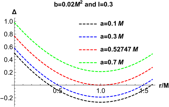
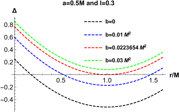
Figure 1: The left one gives variation of $\Delta$ for various values of $a$ with $b=0.02M^{2}$ and $l=0.3$, and the right one gives variation for various values of $b$ with $a=0.5M$ and $l=0.3$.

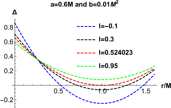
Figure 2: It gives variation of $\Delta$for various values of $l$ with $b=0.01M^{2}$ and $a=0.6$.

From the above plots we see that there exists critical values of $a$, for fixed values of $b$ and $l$, critical values of $b$ for fixed values of $a,l$ and critical values of $l$ for fixed values of $b,a$. The critical value of $a$, $b$ and $l$ are designated by $a_{c},b_{c}$ and $l_{c}$ respectively. In these cases $\Delta=0$ has only one root. For $a<a_{c}$ we have black hole and for $a>a_{c}$ we have naked singularity. Similarly for $b<b_{c}$ we have black hole, but for $b>b_{c}$ we have naked singularity and for $l<l_{c}$ signifies the black hole, however $l>l_{c}$ represents the naked singularity. Numerical computation shows that we have $a_{c}=.52747M$ for $b=.02M^{2}$ and $l=.3$. Similarly for $a=.5M$ and $l=.3$ we have $b_{c}=.0223654M^{2}$, and for $a=.6M$ and $b=.01M^{2}$ we find $l_{c}=.524023$.

There exists a black hole when the following inequality is maintained

$$-\pi la^{2}-\pi a^{2}+\pi M^{2}-8\sqrt{\pi}M\sqrt{b}\geq 0,$$ (23)

However when in the equation (23) equality is maintained it corresponds to extremal black holes, and when the equation (23) is strictly greater than $0$ we have non-extremal black holes which have both the Cauchy and Event horizons.

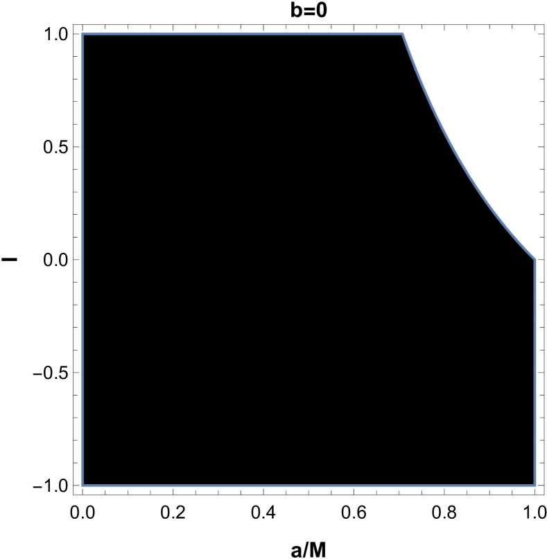
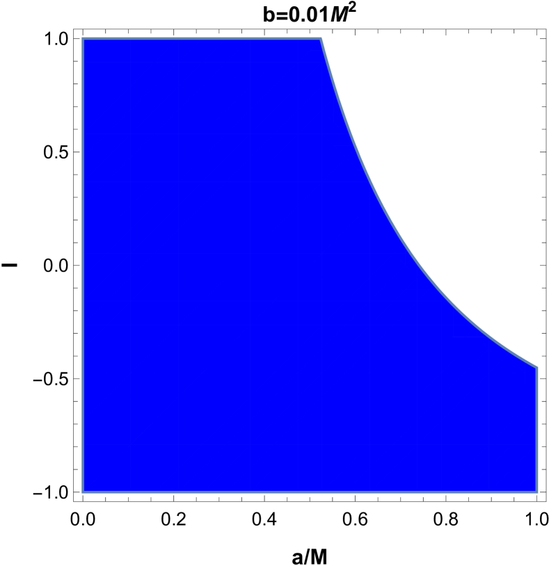
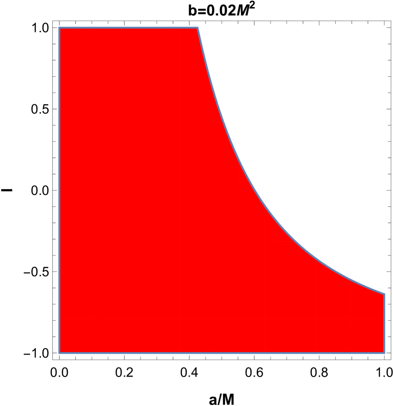
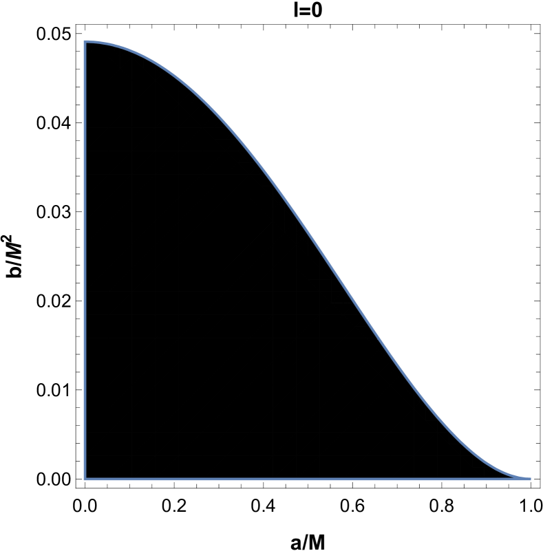
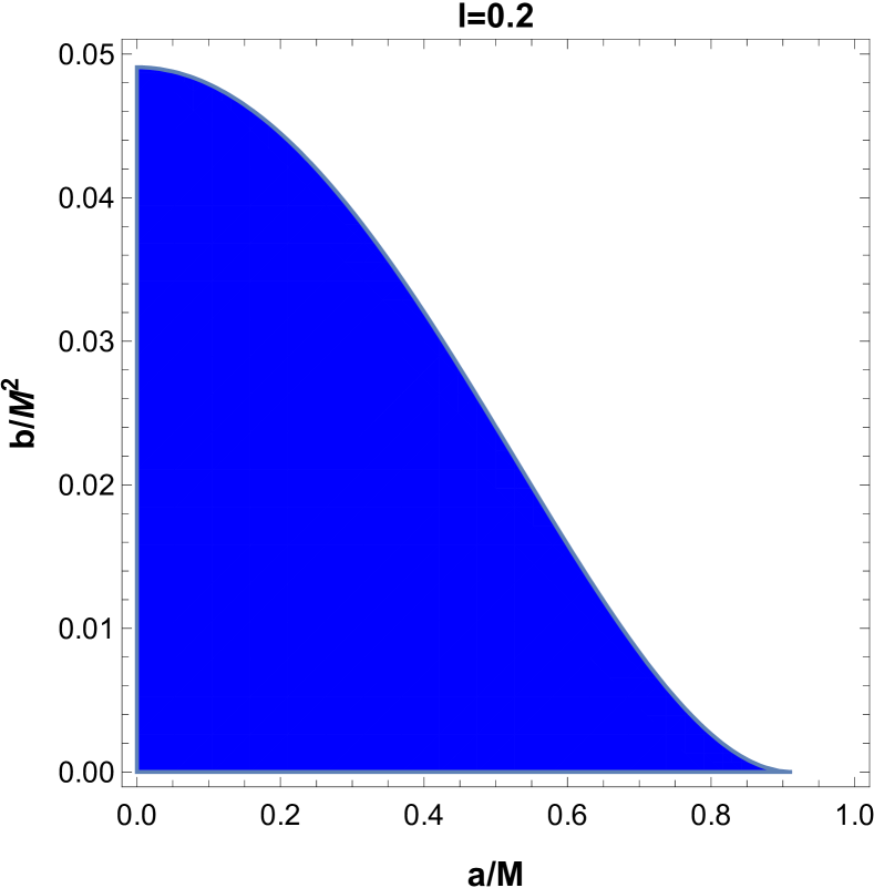
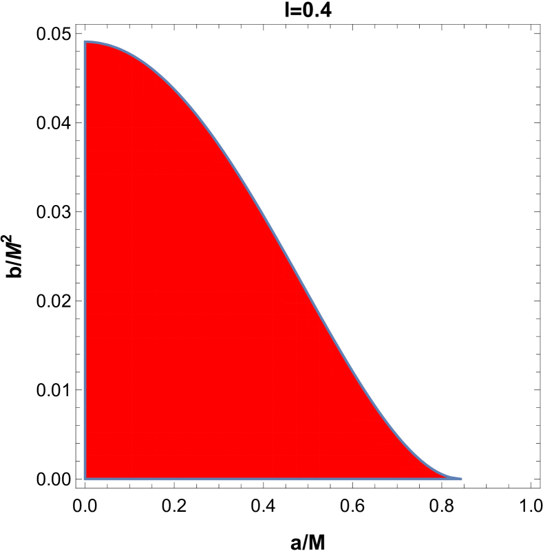
Figure 3: The upper one is the parameter space $(a/M-l)$ for various values of $b$ and the lower one is the parameter space $(a/M-b/M^{2})$ for various values of $l$. The colored regions correspond to parameter space for which we have a black hole.

From the above plots, we observe that as $l$ increases the parameter space $(a/M-b/M^{2})$ for which we have black hole gets shrunk and as $b$ increases the parameter space $(a/M-l)$ for which we have black hole also reduces.

Let us now focus on the static limit surface (SLS). At the SLS, the asymptotic time-translational Killing vector becomes null which is mathematically given by

$$g_{tt}=\rho^{2}-2M_{b}r=0.$$ (24)

The real positive solutions of the above equation give radial coordinates of ergosphere:

$$r^{ergo}_{\pm}=\frac{2\sqrt{\pi}M\pm\sqrt{-4\pi a^{2}\cos^{2}(\theta)-4\pi a^{2}l\cos^{2}(\theta)+4\pi M^{2}-32\sqrt{\pi}M\sqrt{b}}}{2\sqrt{\pi}}.$$ (25)

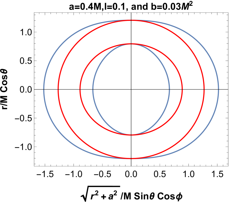
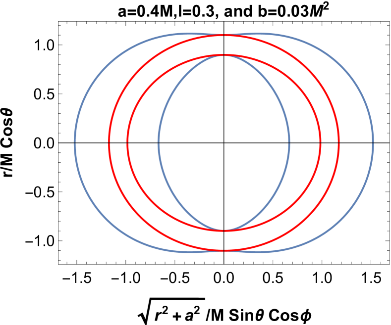
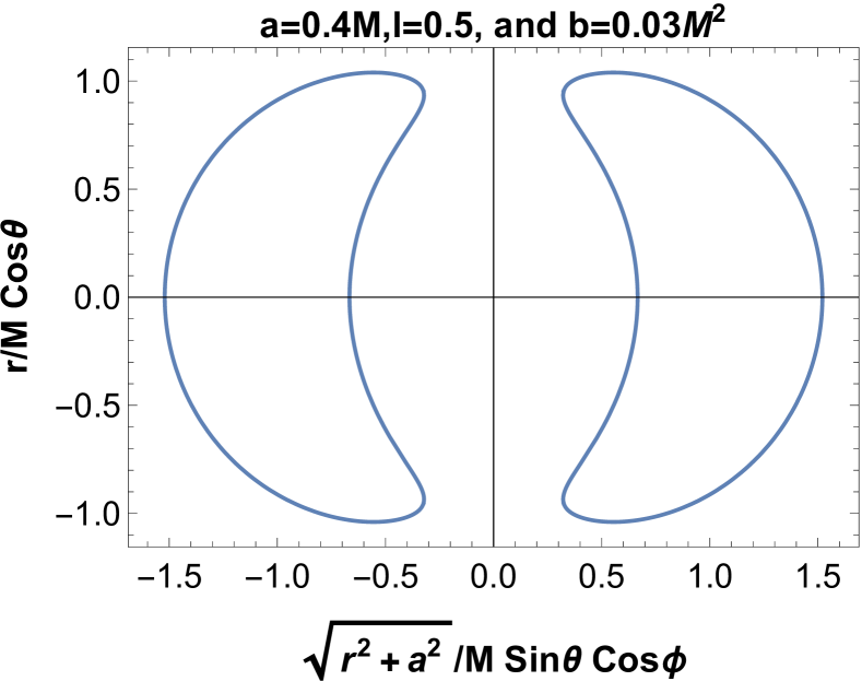
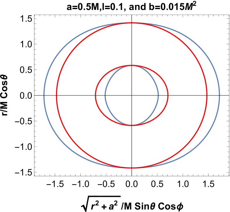
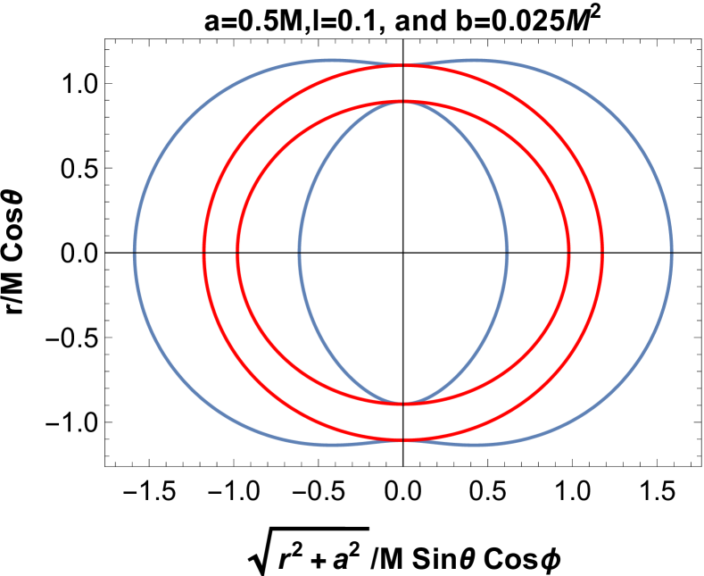
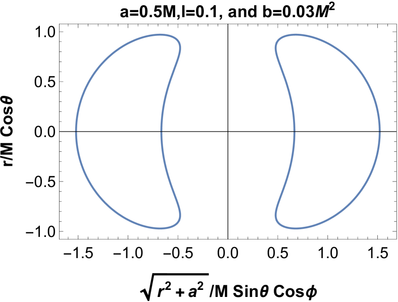
Figure 4: The cross-section of the event horizon (outer red line), SLS (outer blue dotted line), and ergoregion of non-commutative Kerr-like black holes.

The ergosphere, which lies between SLS and the event horizon, is depicted above. Energy can be extracted from ergosphere PENROSE . From the above, we can conclude that the shape and size of the ergosphere depend on rotational parameter $a$, non-commutative parameter $b$, and LV parameter $l$. The size of the ergosphere increases with the increase of $b$ and $l$. This completes our discussion concerning the geometrical structure of this spacetime. Let us now turn toward our main part of the investigation which is connected to the optical properties in the viscidity of this black hole. To this end let us first consider the superradiance phenomena.

IV Superradiance scattering of the scalar field off non-commutative Kerr-like black hole

We bring the Klein-Gordon equation to curved spacetime into action to study the superradiance scattering of a scalar field $\Phi$.

$$\left(\bigtriangledown_{\alpha}\bigtriangledown^{\alpha}+\mu^{2}\right)\Phi(t,r,\theta,\phi)=\left[\frac{-1}{\sqrt{-g}}\partial_{\sigma}\left(g^{\sigma\tau}\sqrt{-g}\partial_{\tau}\right)+\mu^{2}\right]\Phi(t,r,\theta,\phi) = 0.$$ (26)

Here $\mu$ represents the mass of the scalar field $\Phi$. We now adopt the standard separation of variables method to the equation Eqn.(26) in order to separate it into radial and angular part using the following ansatz. With the standard Boyer-Lindquist coordinates $(t,r,\theta,\phi)$ we can write

$$\Phi(t,r,\theta,\phi)=R_{\omega jm}(r)\Theta(\theta)e^{-i\omega t}e^{im\phi},\quad j\geq 0,\quad-j\leq m\leq j,\quad\omega>0,$$ (27)

where $R_{\omega jm}(r)$ represents the radial function and $\Theta(\theta)$ refers to the oblate spheroidal wave function. The symbols $j$, $m$, and $\omega$ respectively stand for the angular eigenfunction, angular quantum number, and the positive frequency of the field under investigation as viewed by a far away observer. Using the ansatz (27), the differential equation (26) is found to get separated into the followingtwo ordinary differential equations. For radial part the equation reads

$$\frac{d}{dr}(\Delta\frac{dR_{\omega jm}(r)}{dr})+(\frac{((r^{2}+a^{2}(1+\ell))\omega-am\sqrt{1+\ell})^{2}}{\Delta(1+\ell)})R_{\omega lm}(r)$$

$$-(\mu^{2}r^{2}+j(j+1)+a^{2}(1+\ell)\omega^{2}-2m\omega a\sqrt{1+\ell})R_{\omega lm}(r)=0,$$ (28)

and the angular part of it is

$$\sin\theta\frac{d}{d\theta}\left(\sin\theta\frac{d\Theta_{\omega jm}(\theta)}{d\theta}\right)+\left(j(j+1)\sin^{2}\theta-\left(\left(a\sqrt{1+\ell}\omega\sin^{2}\theta-m\right)^{2}\right)\right)\Theta_{\omega jm}(\theta)$$

$$+a^{2}(1+\ell)\mu^{2}\sin^{2}\theta\cos^{2}\theta~{}\Theta_{\omega jm}(\theta)=0.$$ (29)

Following the earlier investigation BEZERRA ; KRANIOTIS we may have a general solution of the radial equation (28). However, we are intended to study the scattering of the field $\Phi$. So in this situation, we have used the asymptotic matching procedure used in STRO1 ; STRO2 ; TEUK ; PAGE ; RAN . The road map of the important contributions STRO1 ; STRO2 ; TEUK ; PAGE ; MK ; RAN led us reach to the required result without using the general solution. First of all we consider the radial part of the equation (28) to find an asymptotic solution. Use of Regge-Wheeler-like coordinate $r_{*}$ is helpful in this situation in order to deal with the radial equation as per our requirement, which is given by

$$r_{*}\equiv\int dr\frac{r^{2}+a^{2}(1+\ell)}{\Delta},\quad\left(r_{*}\rightarrow-\infty\quad\text{at event horizon},\quad r_{*}\rightarrow\infty\quad\text{at infinity}\right).$$ (30)

To have the equation into the desired shape, we take on a new radial function $\mathcal{R}_{\omega jm}\left(r_{*}\right)=\sqrt{r^{2}+a^{2}(1+\ell)}R_{\omega jm}(r)$. A few steps of algebra, leads us to obtain the radial equation with our desired form.

$$\frac{d^{2}\mathcal{R}_{\omega lm}\left(r_{*}\right)}{dr_{*}^{2}}+V_{\omega jm}(r)\mathcal{R}_{\omega jm}\left(r_{*}\right)=0.$$ (31)

An effective potential takes entry into the picture now and that has the crucial role on the scattering that reads

$$V_{\omega jm}(r) = \frac{1}{1+\ell}\left(\omega-\frac{m\hat{a}}{r^{2}+\hat{a}^{2}}\right)^{2}-\frac{\Delta}{\left(r^{2}+\hat{a}^{2}\right)^{2}}\left[\right.j(j+1)+\hat{a}^{2}\omega^{2}-2m\hat{a}\omega+\mu^{2}r^{2}$$

$$\left.+\sqrt{r^{2}+\hat{a}^{2}}\frac{d}{dr}\left(\frac{r\Delta}{\left(r^{2}+\hat{a}^{2}\right)^{\frac{3}{2}}}\right)\right],$$

where $\hat{a}=a(1+\ell)^{\frac{1}{2}}$. So it appears that it is equivalent to the study of the scattering of the scalar field $\Phi$ under this effective potential (IV). It is beneficial to study the asymptotic behavior of the scattering potential at the event horizon and at spatial infinity in this regard. The potential at the event horizon in the asymptotic limit simplifies into

$$\lim_{r\rightarrow r_{eh}}V_{\omega jm}(r)=\frac{1}{1+\ell}\left(\omega-m\hat{\Omega}_{h}\right)^{2}\equiv k_{eh}^{2}.$$ (33)

and the same at spatial infinity turns into the following after a few step of algebra

$$\lim_{r\rightarrow\infty}V_{\omega jm}(r)=\frac{\omega^{2}}{1+\ell}-\lim_{r\rightarrow\infty}\frac{\mu^{2}r^{2}\Delta}{\left(r^{2}+\tilde{a}^{2}\right)^{2}}=\frac{\omega^{2}}{1+\ell}-\hat{\mu}^{2}\equiv k_{\infty}^{2},~{}~{}~{}\hat{\mu}=\frac{\mu}{\sqrt{\ell+1}}.$$ (34)

Note that the potential turns into a constant at the two extremal points namely at event horizon and at spatial infinity, however, the numerical values of the constants are different indeed at the two extremal points.

Since the behavior of the potential at the two extremal points are known, we now move to observe the asymptotic behavior of the radial solution. A little algebra shows that the radial equation (31) has the following solutions

$$R_{\omega jm}(r)\rightarrow\left\{\begin{array}[]{cl}\frac{\mathcal{D}_{in}^{eh}e^{-ik_{eh}r_{*}}}{\sqrt{r_{eh}^{2}+\hat{a}^{2}}}&\text{ for }r\rightarrow r_{eh}\\ \mathcal{D}_{in}^{\infty}\frac{e^{-ik_{\infty}r_{*}}}{r}+\mathcal{D}_{ref}^{\infty}\frac{e^{ik_{\infty}r_{*}}}{r}&\text{ for }r\rightarrow\infty\end{array}\right\}$$ (35)

in the asymptotic limit. Here $\mathcal{D}_{in}^{eh}$ be the amplitude of the incoming scalar wave at event horizon($r_{eh}$), and $\mathcal{D}_{in}^{\infty}$ is the corresponding quantity of the incoming scalar wave at infinity $(\infty)$. The amplitude of the reflected part of scalar wave at infinity $(\infty)$ is designated by $\mathcal{D}_{ref}^{\infty}$. So the stage is set to compute the Wronskian for the region adjacent to the event horizon and at infinity. The Wronskian for the event horizon is found out to be

$$W_{eh}=\left(R_{\omega jm}^{eh}\frac{dR_{\omega jm}^{*eh}}{dr_{*}}-R_{\omega jm}^{*eh}\frac{dR_{\omega jm}^{eh}}{dr_{*}}\right),$$ (36)

and the Wronskian at infinity results out to

$$W_{\infty}=\left(R_{\omega jm}^{\infty}\frac{dR_{\omega jm}^{*\infty}}{dr_{*}}-R_{\omega jm}^{*\infty}\frac{dR_{\omega jm}^{\infty}}{dr_{*}}\right).$$ (37)

The knowledge of standard theory of ordinary differential equation provides the information that the Wronskian corresponding to the solutions will be independent of $r^{*}$ since the solution are linearly independent. Thus, the Wronskian evaluated at horizon is compatible to equate with the Wronskian evaluated at infinity. In fact, in the physical sense, it is associated with the flux conservation of the process REVIEW . From the matching condition an important relation between the amplitudes of incoming and reflected waves at different regions of interest results.

$$\left|\mathcal{D}_{ref}^{\infty}\right|^{2}=\left|\mathcal{D}_{in}^{\infty}\right|^{2}-\frac{k_{eh}}{k_{\infty}}\left|\mathcal{D}_{in}^{eh}\right|^{2}.$$ (38)

A careful look reveals that if $\frac{k_{eh}}{k_{\infty}}<0$ i.e., $\omega<m\hat{\Omega}_{eh}$, the scalar wave will be superradiantly amplified, since the relation $\left|\mathcal{D}_{ref}^{\infty}\right|^{2}>\left|\mathcal{D}_{in}^{\infty}\right|^{2}$ holds explicitly in this situation.

IV.1 Amplification factor $Z_{jm}$ for superradiance

It is straightforward to express the radial equation (28) in the following form

$$\Delta^{2}\frac{d^{2}R_{\omega jm}(r)}{dr^{2}}+\Delta\frac{d\Delta}{dr}\cdot\frac{dR_{\omega jm}(r)}{dr}$$

$$+\left(\frac{\left(\left(r^{2}+\hat{a}^{2}\right)\omega-\hat{a}m\right)^{2}}{1+\ell}-\Delta\left(\mu^{2}r^{2}+j(j+1)+\hat{a}^{2}\omega^{2}-2m\hat{a}\omega\right)\right)R_{\omega jm}(r)=0.$$ (39)

We now proceed to derive the solution for the near and the far region and try to find out a single solution by matching the solution for near-region at infinitely with solution for the far-region at its initial point such that this specific single solution be useful in the vicinity of the cardinal region. it is beneficial at this stage to introduce a a new variable $y$ which is defined by $y=\frac{r-r_{eh}}{r_{eh}-r_{ch}}$. In terms of $y$ the equation (39) turns into

$$\frac{y^{2}(y+1)^{2}}{(\ell+1)^{2}}\frac{\mathrm{d}^{2}R_{\omega jm}(y)}{\mathrm{d}y^{2}}+\frac{y(y+1)(2y+1)}{(\ell+1)^{2}}\frac{\mathrm{d}R_{\omega jm}(y)}{\mathrm{d}y}$$ (40)

$$+\left(\frac{\mathcal{Q}^{2}y^{4}}{1+\ell}+\frac{B^{2}}{1+\ell}-\frac{j(j+1)}{\ell+1}y(y+1)-\frac{\hat{\mu}^{2}\mathcal{Q}^{2}}{\omega^{2}}y^{3}(y+1)-\hat{\mu}^{2}r_{eh}^{2}y(y+1)-\frac{2\hat{\mu}^{2}r_{eh}\mathcal{Q}}{\omega}y^{2}(y+1)\right)R_{\omega jm}(y)=0,$$

Under under the approximation $\hat{a}\omega\ll 1$, where $\mathcal{Q}=\left(r_{eh}-r_{ch}\right)\omega$ and $B=\frac{(\omega-m\hat{\Omega})}{r_{eh}-r_{ch}}r_{eh}^{2}$. For the near-region, we have $Py\ll 1$ and $\hat{\mu}^{2}r_{eh}^{2}\ll 1$. The above equation is simplified into

$$y^{2}(y+1)^{2}\frac{\mathrm{d}^{2}R_{\omega jm}(y)}{\mathrm{d}y^{2}}+y(y+1)(2y+1)\frac{\mathrm{d}R_{\omega jm}(y)}{\mathrm{d}y}+\left((\ell+1)B^{2}-j(j+1)(\ell+1)y(y+1)\right)R_{\omega jm}(r)=0.$$ (41)

Since the Compton wavelength of the boson participating in the scattering process is much smaller than the size of the black hole the approximation $\left(\hat{\mu}^{2}r_{eh}^{2}\ll 1\right)$ holds good. The general solution of the above equation in terms of associated Legendre function of the first kind $P_{\lambda}^{\nu}(y)$ can be written down as

$$R_{\omega jm}(y)=dP^{2i\sqrt{1+\ell}B}_{\frac{\sqrt{1+4j(j+1)(l+1)}-1}{2}}(1+2y).$$ (42)

If we now use the relation

$$P_{\lambda}^{\nu}(z)=\frac{1}{\Gamma(1-\nu)}\left(\frac{1+z}{1-z}\right)^{\nu/2}{}_{2}F_{1}\left(-\lambda,\lambda+1;1-\nu;\frac{1-z}{2}\right).$$ (43)

it enables us to express $R_{\omega jm}(y)$ in terms of the ordinary hypergeometric functions ${}_{2}F_{1}(a,b;c;z)$ :

$$R_{\omega jm}(y)=d\left(\frac{y}{y+1}\right)^{-i\sqrt{\ell+1}B}{}_{2}F_{1}\left(\frac{1-\sqrt{1+4(\ell+1)j(j+1)}}{2},\frac{1+\sqrt{1+4(\ell+1)j(j+1)}}{2};1-2i\sqrt{\ell+1}B;-y\right).$$ (44)

We are intended to find out a single solution using the matching condition at the desired position where the two solutions mingle with each other. In this respect, we need to observe the large $y$ behavior of the above expression. The Eqn. (44) for large y, i.e.,$(y\to\infty$) reduces to

$$R_{\text{near-large }y}\sim d \left(\frac{\Gamma(\sqrt{1+4(\ell+1)j(j+1)})\Gamma(1-2i\sqrt{\ell+1}B)}{\Gamma\left(\frac{1+\sqrt{1+4(\ell+1)j(j+1)}}{2}-2i\sqrt{\ell+1}B\right)\Gamma\left(\frac{1+\sqrt{1+4(\ell+1)j(j+1)}}{2}\right)}y^{\frac{\sqrt{1+4(\ell+1)j(j+1)}-1}{2}}+\right.$$ (46)

$$\frac{\Gamma(-\sqrt{1+4(\ell+1)j(j+1)})\Gamma(1-2i\sqrt{\ell+1}B)}{\Gamma\left(\frac{1-\sqrt{1+4(\ell+1)j(j+1)}}{2}\right)\Gamma\left(\frac{1-\sqrt{1+4(\ell+1)j(j+1)}}{2}-2i\sqrt{\ell+1}B\right)}y^{\left.-\frac{\sqrt{1+4(\ell+1)j(j+1)}+1}{2}\right)}.$$

For the far-region, we can use the approximations $y+1\approx y$ and $\hat{\mu}^{2}r_{eh}^{2}\ll 1$. We may drop all the terms except those which describe the free motion with momentum $j$ and that reduces equation (39) to

$$\frac{\mathrm{d}^{2}R_{\omega jm}(y)}{\mathrm{d}y^{2}}+\frac{2}{y}\frac{\mathrm{d}R_{\omega jm}(y)}{\mathrm{d}y}+\left(k_{l}^{2}-\frac{j(j+1)(\ell+1)}{y^{2}}\right)R_{\omega jm}(y)=0,$$ (47)

where $k_{l}\equiv\frac{P\sqrt{1+\ell}}{\omega}\sqrt{\omega^{2}-\mu^{2}}$. Equation (47) has the general solution

$$R_{\omega jm,\text{ far }}=e^{-iky}(c_{1}y^{\frac{\sqrt{1+4(\ell+1)j(j+1)}-1}{2}}M(\frac{1+\sqrt{1+4(\ell+1)j(j+1)}}{2},1+\sqrt{1+4(\ell+1)l(l+1)},2ik_{l}y)+$$ (48)

$$c_{2}y^{-\frac{\sqrt{1+4(\alpha+1)j(j+1)}+1}{2}}M(\frac{1-\sqrt{1+4(\ell+1)j(j+1)}}{2},1-\sqrt{1+4(\ell+1)j(j+1)},2ik_{l}y)),$$

Here $M(a;b;y)$ stands for the confluent hypergeometric Kummer function of the first kind. In order to match the solution with (46), we look for the small $y$ behavior of the solution (IV.1). The solution (46) and (50) are susceptible for matching, since these two have common region of interest. The matching of the asymptotic solutions (46) and (50) enables us to compute the scalar wave flux at infinity that resulting in

$$c_{1}= d\frac{\Gamma(\sqrt{1+4(\ell+1)j(j+1)})\Gamma(1-2i\sqrt{\ell+1}B)}{\Gamma\left(\frac{1+\sqrt{1+4(\ell+1)j(j+1)}}{2}-2i\sqrt{\ell+1}B\right)\Gamma\left(\frac{1+\sqrt{1+4(\ell+1)j(j+1)}}{2}\right)},$$ (49)

$$c_{2}= d\frac{\Gamma(-\sqrt{1+4(\ell+1)j(j+1)})\Gamma(1-2i\sqrt{\ell+1}B)}{\Gamma\left(\frac{1-\sqrt{1+4(\ell+1)j(j+1)}}{2}-2i\sqrt{\ell+1}B\right)\Gamma\left(\frac{1-\sqrt{1+4(\ell+1)j(j+1)}}{2}\right)}.$$

For small $y(y\to 0)$, the equation (IV.1) turns into

$$R_{\omega jm,\text{ far-small }\mathrm{y}}\sim y^{-\frac{1+\sqrt{1+4(\ell+1)j(j+1)}}{2}}.$$ (50)

Since these two solutions (46), and (50) have a common region of interest, the solutions are susceptible for matching. We therefore compute the scalar wave flux at infinity resulting by matching the asymptotic solutions (46) and

$$c_{1}= d\frac{\Gamma(\sqrt{1+4(\ell+1)j(j+1)})\Gamma(1-2i\sqrt{\ell+1}B)}{\Gamma\left(\frac{1+\sqrt{1+4(\ell+1)j(j+1)}}{2}-2i\sqrt{\ell+1}B\right)\Gamma\left(\frac{1+\sqrt{1+4(\ell+1)j(j+1)}}{2}\right)},$$ (51)

$$c_{2}= d\frac{\Gamma(-\sqrt{1+4(\ell+1)j(j+1)})\Gamma(1-2i\sqrt{\ell+1}B)}{\Gamma\left(\frac{1-\sqrt{1+4(\ell+1)j(j+1)}}{2}-2i\sqrt{\ell+1}B\right)\Gamma\left(\frac{1-\sqrt{1+4(\ell+1)j(j+1)}}{2}\right)}.$$

We expand equation (IV.1) around infinity which after expansion results

$$c_{1}\frac{\Gamma(1+\sqrt{1+4(\ell+1)j(j+1)})}{\Gamma\left(\frac{1+\sqrt{1+4(\ell+1)j(j+1)}}{2}\right)}k_{l}^{-\frac{1+\sqrt{1+4(\ell+1)j(j+1)}}{2}}\left((-2i)^{-\frac{1+\sqrt{1+4(\ell+1)j(j+1)}}{2}}\frac{e^{-ik_{l}y}}{y}+(2i)^{-\frac{1+\sqrt{1+4(\ell+1)j(j+1)}}{2}}\frac{e^{ik_{l}y}}{y}\right)+$$ (52)

$$c_{2}\frac{\Gamma(1-\sqrt{1+4(\ell+1)j(j+1)})}{\Gamma\left(\frac{1-\sqrt{1+4(\ell+1)j(j+1)}}{2}\right)}k_{l}^{\frac{\sqrt{1+4(\ell+1)j(j+1)}-1}{2}}\left((-2i)^{\frac{\sqrt{1+4(\ell+1)j(j+1)}-1}{2}}\frac{e^{-ik_{l}y}}{y}+(2i)^{\frac{\sqrt{1+4(\ell+1)j(j+1)}-1}{2}}\frac{e^{ik_{l}y}}{y}\right).$$

With the approximations $\frac{1}{y}\sim\frac{\mathcal{Q}}{\omega}\cdot\frac{1}{r},\quad e^{\pm ik_{l}y}\sim e^{\pm i\sqrt{(1+\ell)(\omega^{2}-\mu^{2})}r}$, if we match the above solution with the radial solution (35)

$$R_{\infty}(r)\sim\mathcal{D}_{in}^{\infty}\frac{e^{-i\sqrt{\frac{\omega^{2}}{1+\ell}-\hat{\mu}^{2}}r^{*}}}{r}+\mathcal{D}_{ref}^{\infty}\frac{e^{i\sqrt{\frac{\omega^{2}}{1+\ell}-\hat{\mu}^{2}}r^{*}}}{r},\quad\text{ for }\quad r\rightarrow\infty$$

we get

$$\begin{array}[]{c}\mathcal{D}_{in}^{\infty}=\frac{\mathcal{Q}}{\omega}\left(c_{1}(-2i)^{-\frac{1+\sqrt{1+4(\ell+1)j(j+1)}}{2}}\frac{\Gamma(1+\sqrt{1+4(\ell+1)j(j+1)})}{\Gamma\left(\frac{1+\sqrt{1+4(\ell+1)j(j+1)}}{2}\right)}k_{l}^{-\frac{1+\sqrt{1+4(\ell+1)j(j+1)}}{2}}+\right.\\ \left.c_{2}(-2i)^{\frac{\sqrt{1+4(\ell+1)j(j+1)}-1}{2}}\frac{\Gamma(1-\sqrt{1+4(\ell+1)j(j+1)})}{\Gamma\left(\frac{1-\sqrt{1+4(\ell+1)j(j+1)}}{2}\right)}k_{l}^{\frac{\sqrt{1+4(\ell+1)j(j+1)}-1}{2}}\right),\end{array}$$

and

$$\begin{array}[]{l}\mathcal{D}_{ref}^{\infty}=\frac{\mathcal{Q}}{\omega}\left(c_{1}(2i)^{-\frac{1+\sqrt{1+4(\ell+1)j(j+1)}}{2}}\frac{\Gamma(1+\sqrt{1+4(\ell+1)j(j+1)})}{\Gamma\left(\frac{1+\sqrt{1+4(\ell+1)j(j+1)}}{2}\right)}k_{l}^{-\frac{1+\sqrt{1+4(\ell+1)j(j+1)}}{2}}+\right.\\ \left.c_{2}(2i)\frac{\sqrt{1+4(\ell+1)j(j+1)}-1}{2}\frac{\Gamma(1-\sqrt{1+4(\ell+1)j(j+1)})}{\Gamma\left(\frac{1-\sqrt{1+4(\ell+1)j(j+1)}}{2}\right)}k_{l}^{\frac{\sqrt{1+4(\ell+1)j(j+1)}-1}{2}}\right).\end{array}$$

Substituting the expressions of $c_{1}$ and $c_{2}$ from Eqn. (IV.1) into the above expressions we have

$$\mathcal{D}_{in}^{\infty} = \frac{d(-2i)^{-\frac{1+\sqrt{1+4(\ell+1)j(j+1)}}{2}}}{\sqrt{(1+\ell)(\omega^{2}-\mu^{2})}}\cdot\frac{\Gamma(\sqrt{1+4(\ell+1)j(j+1)})\Gamma(1+\sqrt{1+4(\ell+1)j(j+1)})}{\Gamma\left(\frac{1+\sqrt{1+4(\ell+1)j(j+1)}}{2}-2i\sqrt{\ell+1}B\right)\left(\Gamma\left(\frac{1+\sqrt{1+4(\ell+1)j(j+1)}}{2}\right)\right)^{2}}\times$$

$$\Gamma(1-2i\sqrt{\ell+1}B)k_{l}^{\frac{1-\sqrt{1+4(\ell+1)j(j+1)}}{2}}+\frac{d(-2i)^{\frac{\sqrt{1+4(\ell+1)j(j+1)}-1}{2}}}{\sqrt{(1+\ell)(\omega^{2}-\hat{\mu}^{2})}}\times$$

$$\frac{\Gamma(1-\sqrt{1+4(\ell+1)j(j+1)})\Gamma(-\sqrt{1+4(\ell+1)j(j+1)})}{\left(\Gamma\left(\frac{1-\sqrt{1+4(\ell+1)j(j+1)}}{2}\right)\right)^{2}\Gamma\left(\frac{1-\sqrt{1+4(\ell+1)j(j+1)}}{2}-2i\sqrt{\ell+1}B\right)}\Gamma(1-2i\sqrt{\ell+1}B)k_{l}^{\frac{1+\sqrt{1+4(\ell+1)j(j+1)}}{2}},$$

and

$$\mathcal{D}_{ref}^{\infty} = \frac{d(2i)^{-\frac{1+\sqrt{1+4(\ell+1)j(j+1)}}{2}}}{\sqrt{(1+\ell)(\omega^{2}-\mu^{2})}}\cdot\frac{\Gamma(\sqrt{1+4(\ell+1)j(j+1)})\Gamma(1+\sqrt{1+4(\ell+1)j(j+1)})}{\Gamma\left(\frac{1+\sqrt{1+4(\ell+1)j(j+1)}}{2}-2i\sqrt{\ell+1}B\right)\left(\Gamma\left(\frac{1+\sqrt{1+4(\ell+1)j(j+1)}}{2}\right)\right)^{2}}\times$$

$$\Gamma(1-2i\sqrt{\ell+1}B)k_{l}^{\frac{1-\sqrt{1+4(\ell+1)j(j+1)}}{2}}+\frac{d(2i)^{\frac{\sqrt{1+4(\ell+1)j(j+1)}-1}{2}}}{\sqrt{(1+\ell)(\omega^{2}-\hat{\mu}^{2})}}\times$$

$$\frac{\Gamma(1-\sqrt{1+4(\ell+1)j(j+1)})\Gamma(-\sqrt{1+4(\ell+1)j(j+1)})}{\left(\Gamma\left(\frac{1-\sqrt{1+4(\ell+1)j(j+1)}}{2}\right)\right)^{2}\Gamma\left(\frac{1-\sqrt{1+4(\ell+1)j(j+1)}}{2}-2i\sqrt{\ell+1}B\right)}\Gamma(1-2i\sqrt{\ell+1}B)k_{l}^{\frac{1+\sqrt{1+4(\ell+1)j(j+1)}}{2}}.$$

The amplification factor ultimately results out to be

$$Z_{jm}\equiv\frac{\left|\mathcal{D}_{ref}^{\infty}\right|^{2}}{\left|\mathcal{D}_{in}^{\infty}\right|^{2}}-1.$$ (55)

Equation (55) is a general expression of the amplification factor obtained by making use of the asymptotic matching method. When $\frac{\left|\mathcal{D}_{ref}^{\infty}\right|^{2}}{\left|\mathcal{D}_{in}^{\infty}\right|^{2}}$ acquires a value greater than unity there will be a gain in amplification factor that corresponds to superradiance phenomena. However, a negative value of the amplification factor indicates a loss that corresponds to the non-appearance of superradiance. To study the effect of Lorentz violation on the superradiance phenomena, it will be useful to plot $Z_{jm}$ versus $M\omega$ for different LV parameters. In Fig. (6), we present the variation $Z_{jm}$ versus $M\omega$ for the leading multipoles $j=1$, and $2$ taking different values (both negative and positive) of LV Parameter. From the fig. (5) along with fig. (6), it is evident that superradiance for a particular $j$ occurs when the allowed values of $m$ are restricted to $m>0$.

For negative $m$, amplification factor takes negative value which refers to the nonoccurrence of superradiance. The plots also show transparently that with the decrease in the value of the LV parameters the superradiance process enhances and the reverse is the case when the value of the LV parameter decreases. In Fig. (8) we have also studied the effect of the parameter $b$ on the superradiance scenario. It shows that the superradiance scenario gets diminished with the increase in the value of the parameter $b$. In ARS we have noticed that the size of the shadow decreases with the increase in the value of both the parameters $l$ and $b$. The only difference is that $l$ can take both positive values, however, $b$ as per definition can not be negative. Therefore, an indirect relation of superradiance with the size of the shadow is being revealed through this analysis. A decrease in the value of $b$ and $l$ indicate the increase in the size of the shadow.

We observe that for the negative value of $m$, the amplification factor takes negative value. Therefore, superradiance does not occur. The plots also transpires that with the superradiance process enhances with the decrease in the value of the LV parameters, and it diminishes with the increase in value of the LV parameter. In Fig. (8), we have also studied the effect of the parameter $b$ related to the non-commutativity of the sapcetime on the superradiance process. It shows that with the increase in the value of the parameter $b$ the superradiance process gets diminished. However, with the increase in $a$ the superradiance effect increases as is found from Fig.(7).

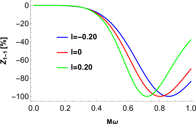
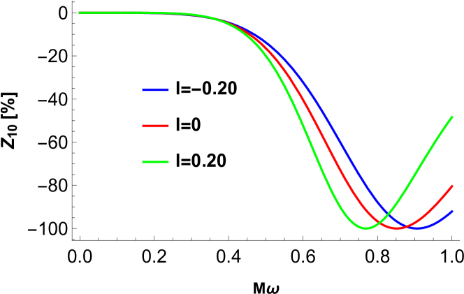
Figure 5: Variation of amplification factors with $\ell$ for non-superradiant multipoles with $\hat{\mu}=0.1,b=0.01M^{2}$, and $\hat{a}=0.3M$.

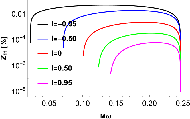
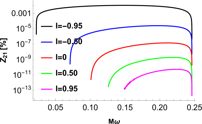
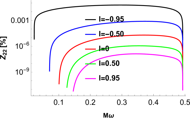
Figure 6: Variation of amplification factors with $\ell$ for various multipoles with $\hat{\mu}=0.1,b=0.02M^{2}$, and $\hat{a}=0.5M$.

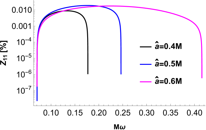
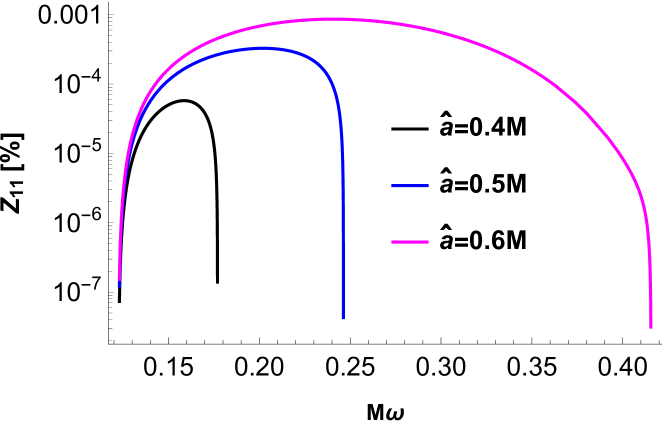
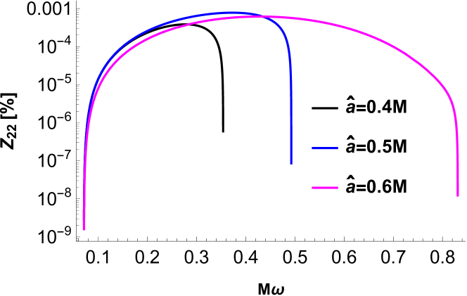
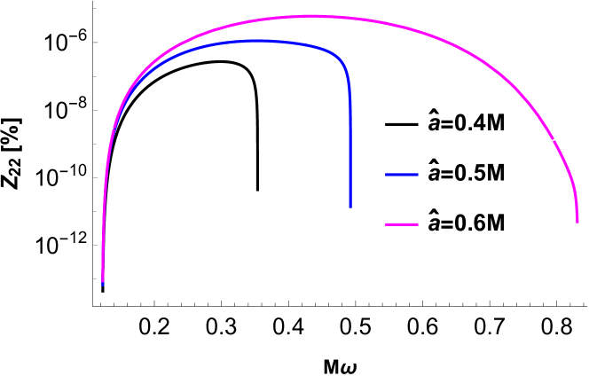
Figure 7: Variation of amplification factors with $\hat{a}$ for various multipoles with $\hat{\mu}=0.1$ and $b=0.02M^{2}$. For left ones $\ell=-0.5$ and for right ones $\ell=0.5$.

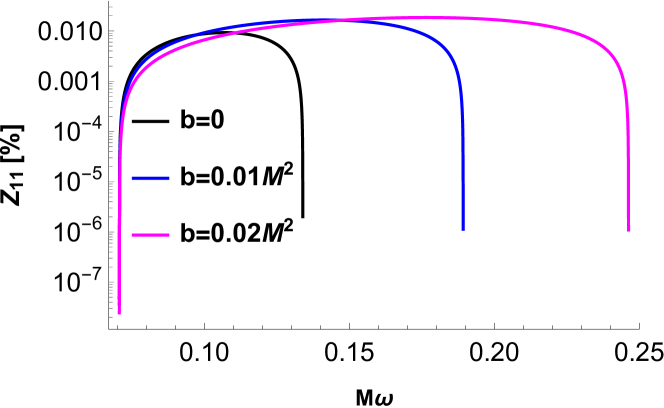
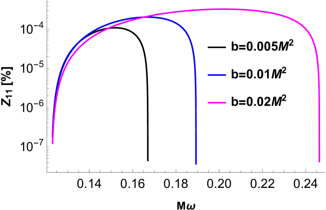
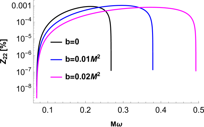
Figure 8: Variation of amplification factors with $b$ for various multipoles with $\hat{\mu}=0.1$ and $\hat{a}=0.5M$. For left ones $\ell=-0.5$ and for right ones $\ell=1$.

IV.2 Superradiant instability for Lorentz violating and non-commutative Kerr-like black hole

From equation (28) we have

$$\Delta\frac{d}{dr}\left(\Delta\frac{dR_{\omega jm}}{dr}\right)+\mathcal{F}R_{\omega jm}=0,$$ (56)

where for a slowly rotating black hole $(\hat{a}\omega\ll 1)$

$$\mathcal{F}\equiv\frac{\left(\left(r^{2}+\hat{a}^{2}\right)\omega-m\hat{a}\right)^{2}}{1+\ell}+\Delta\left(2m\hat{a}\omega-l(l+1)-\mu^{2}r^{2}\right).$$

If we now look for the black hole bomb mechanism, we would have have the following solutions for the radial equation (56)

$$R_{\omega jm}\sim\left\{\begin{array}[]{ll}e^{-i(\omega-m\hat{\Omega})r_{*}}&\text{ as }r\rightarrow r_{eh}\left(r_{*}\rightarrow-\infty\right)\\ \frac{e^{-\sqrt{\mu^{2}-\omega^{2}r_{*}}}}{r}&\text{ as }r\rightarrow\infty\left(r_{*}\rightarrow\infty\right)\end{array}\right.$$

The above solution represents the physical boundary conditions that the scalar wave at the black hole horizon is purely ingoing while at spatial infinity it is decaying exponentially (bounded) solution, provided that $\omega^{2}<\mu^{2}$. With the new radial function

$$\psi_{\omega jm}\equiv\sqrt{\Delta}R_{\omega jm},$$

the radial equation (56) turns into

$$\left(\frac{d^{2}}{dr^{2}}+\omega^{2}-V\right)\psi_{\omega jm}=0.$$

with

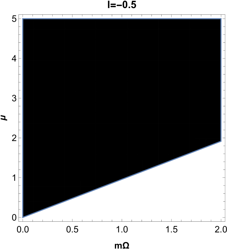
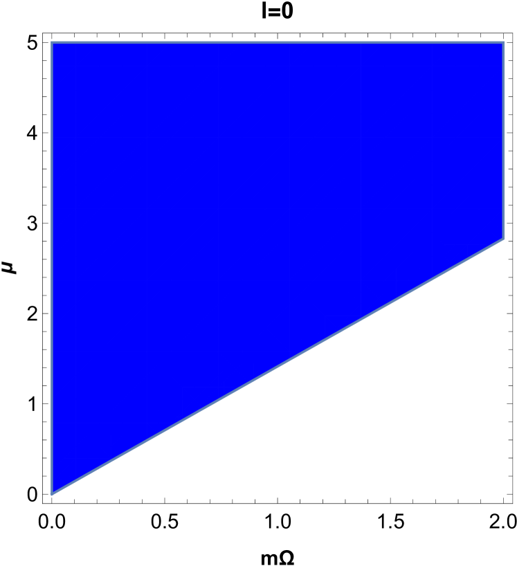
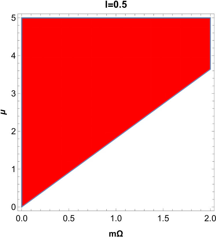
Figure 9: Parameter space($m\Omega$-$\mu$) for massive scalar field where colored area represents region with stable dynamics and non-colored area represents region with unstable dynamics. Here $a=0.4M\quad\text{and}\quad b=0.01M^{2}$

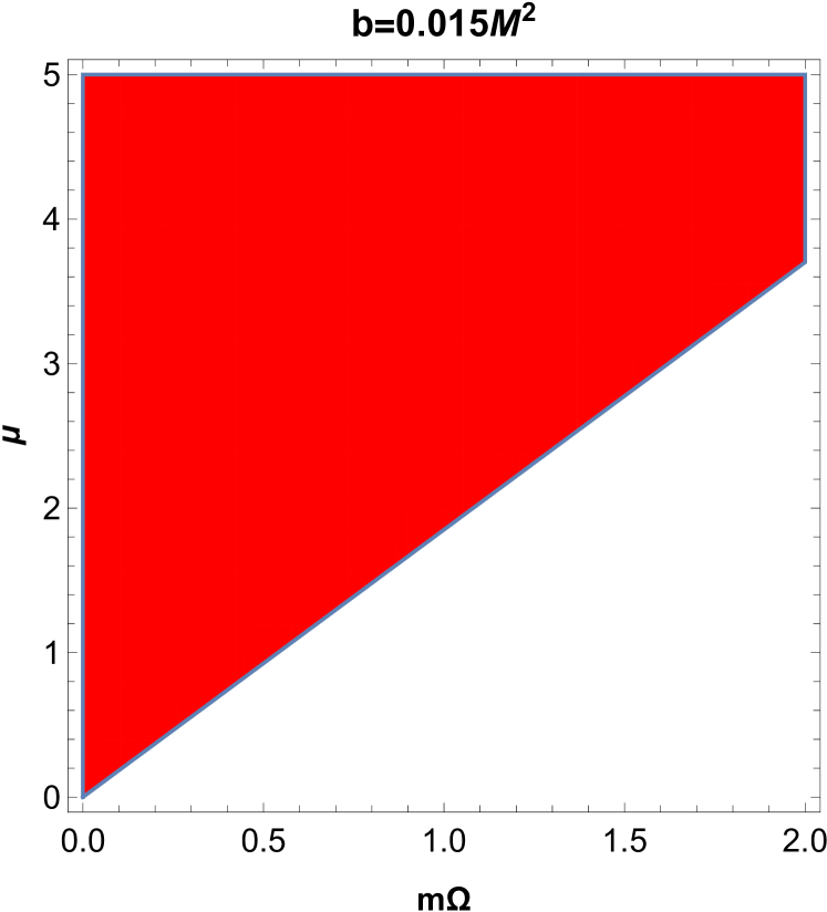
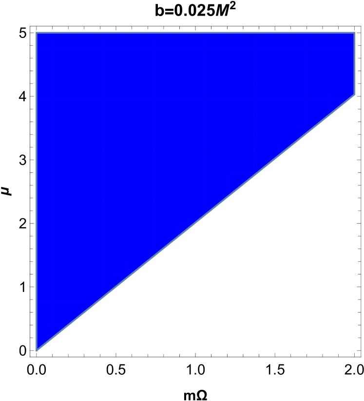
Figure 10: Parameter space($m\Omega$-$\mu$) for massive scalar field where colored area represents region with stable dynamics and non-colored area represents region with unstable dynamics. Here $a=0.4M\quad\text{and}\quad l=0.5$

$$\omega^{2}-V=\frac{\mathcal{F}+\frac{M\left(M-\frac{8\sqrt{t}}{\sqrt{\pi}}\right)-a^{2}(l+1)}{(l+1)^{2}}}{\Delta^{2}},$$

which is the Regge-Wheel equation. By discarding the terms $\mathcal{O}\left(1/r^{2}\right)$ the asymptotic form of the effective potential $V(r)$ looks

$$V(r)=\mu^{2}\left(1+\ell\right)-\left(1+\ell\right)\frac{4M\omega^{2}}{r}+(\ell+1)\frac{2M\mu^{2}}{r}.$$

To realize the trapping meaningfully by the above effective potential it is necessary that its asymptotic derivative be positive i.e. $V^{\prime}\rightarrow 0^{+}$ as $r\rightarrow\infty$ HOD . This along with the fact that superradiance amplification of scattered waves occurs when $\omega<m\hat{\Omega}$ we get the regime

$$\frac{\mu}{\sqrt{2}}<\omega^{2}<m\hat{\Omega},$$

in which the integrated system of non-commutative Kerr bumblebee black hole and massive scalar field may experience a superradiant instability, known as the black hole bomb. The dynamics of the massive scalar field in non-commutative Kerr like black hole will remain stable when $\mu\geq\sqrt{2}m\hat{\Omega}$.

V Photon orbit and black hole shadow

In this section, we study the black hole shadow related to this modified theory. There are several studies related to the black hole shadow from which we will get the necessary inputs for the study SDO1 ; SDO2 ; SDO3 ; SDO4 . In order to study the shadow, we introduce two conserved parameters $\xi$ and $\eta$ as usual which are defined by

$$\xi=\frac{L_{z}}{E}\quad\textrm{and}\quad\eta=\frac{\mathcal{Q}}{E^{2}},$$ (57)

where $E,L_{z}$, and $\mathcal{Q}$ are the energy, the axial component of the angular momentum, and the Carter constant respectively. Then the null geodesics in the bumblebee rotating black hole spacetime in terms of $\xi$ are given by

$$\rho^{2}\frac{dr}{d\lambda}=\pm\sqrt{R},\quad\rho^{2}\frac{d\theta}{d\lambda}=\pm\sqrt{\Theta},$$

$$(1+\ell)\Delta\rho^{2}\frac{dt}{d\lambda}=A-2\sqrt{1+\ell}\operatorname{Mra\xi},$$

$$(1+\ell)\Delta\rho^{2}\frac{d\phi}{d\lambda}=2\sqrt{1+\ell}Mra+\frac{\xi}{\sin^{2}\theta}\left(\rho^{2}-2Mr\right),$$ (58)

where $\lambda$ is the affine parameter and

$$R(r)=\left[\frac{r^{2}+(1+l)a^{2}}{\sqrt{1+l}}-a\xi\right]^{2}-\Delta\left[\eta+(\xi-a\sqrt{1+l})^{2}\right],\quad\Theta(\theta)=\eta+(1+l)a^{2}\cos^{2}\theta-\xi^{2}\cot^{2}\theta.$$ (59)

The radial equation of motion can be written down in the familiar form

$$\left(\rho^{2}\frac{dr}{d\lambda}\right)^{2}+V_{eff}=0.$$ (60)

The effective potential $V_{eff}$ then reads

$$V_{eff}=-\left[\frac{r^{2}+(1+l)a^{2}}{\sqrt{1+l}}-a\xi\right]^{2}+\Delta\left[\eta+(\xi-a\sqrt{1+l})^{2}\right].$$ (61)

The following equations describe the unstable spherical orbit on the equatorial plane, $\theta=\frac{\pi}{2}$.

$$\theta=\frac{\pi}{2},\quad R(r)=0,\quad\frac{dR}{dr}=0,\quad\frac{d^{2}R}{dr^{2}}<0,\quad\textrm{and}\quad\eta=0.$$ (62)

We plot the potential $V_{eff}$ versus $r/M$ with $\xi=\xi_{c}+0.2$, where $\xi_{c}$ is the value of $\xi$ for equatorial spherical unstable orbit.

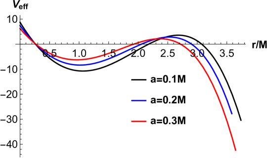
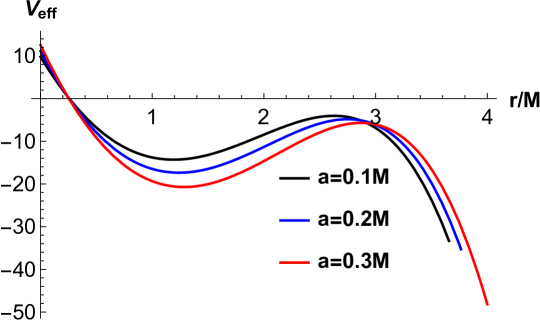
Figure 11: The left and the right panels describe the effective potential for prograde orbits and the retrograde orbits respectively for various values of $a$ with $b=0.01M^{2}$ and $l=0.1$.

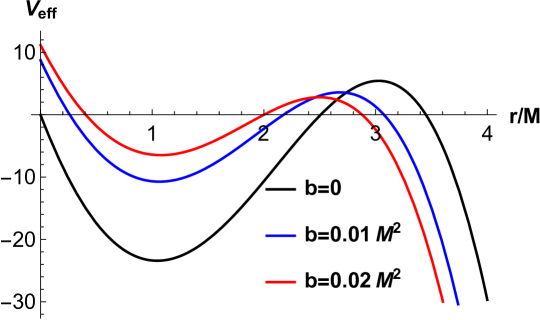
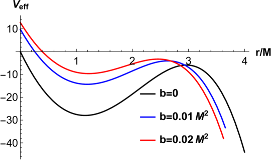
Figure 12: The left and the right panels describe the effective potential for prograde orbits and the retrograde orbits respectively for various values of $b$ with $a=0.1M$ and $l=0.1$.

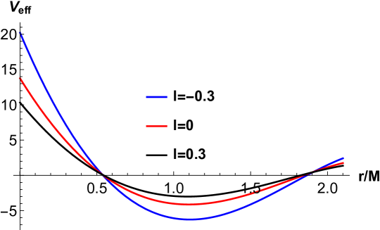
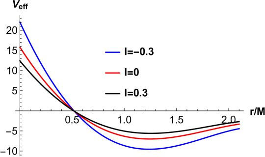
Figure 13: The left panel describes the effective potential for prograde orbits and right panel describes the retrograde orbits for various values of $l$ with $a=0.1M$ and $b=.03M^{2}$.

The plots depicted above show that the turning points for prograde orbits shift towards the left as $a$ or $b$ increases. We also plot-critical radii of prograde and retrograde orbits for the different scenarios in the Fig. furnished below.

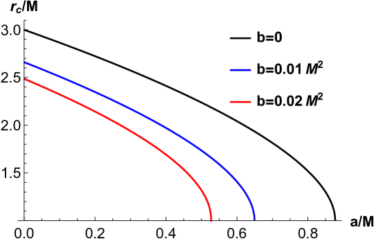
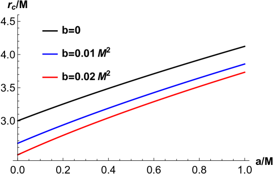
Figure 14: The left panel shows the variation of critical radius for prograde orbits and the right panel shows the variation of critical radius for retrograde orbits for various values of $b$ with $l=0.3$.

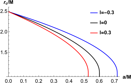
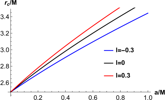
Figure 15: The left panel shows the variation of critical radius for prograde orbits and the right one shows the variation of the critical radius for retrograde orbits for various values of $l$ with $b=0.02M^{2}$.

It can be concluded from the above plots that critical radii, both for the prograde and retrograde orbits, decrease with an increase in the non-commutative parameter $b$. On the other hand, the critical radius for prograde orbit decreases with the increase in $l$ but for retrograde orbit, it increases with the increase in $l$. For more generic orbits $\theta\neq\pi/2$ and $\eta\neq 0,$ the solution of Eqn. (62)$r=r_{s}$, gives the $r-$ constant orbit, which is also called spherical orbit and the conserved parameters of the spherical orbits are given by

$$\xi_{s} = \frac{\left(a^{2}\left(1+l\right)+r^{2}\right)\Delta^{{}^{\prime}}(r)-4r\Delta(r)}{a\sqrt{1+l}\Delta^{{}^{\prime}}(r)},$$ (63)

$$\eta_{s} = \frac{r^{2}\left(8\Delta(r)\left(2a^{2}\left(1+l\right)+r\Delta^{{}^{\prime}}(r)\right)-r^{2}\Delta^{{}^{\prime}}(r)^{2}-16\Delta^{{}^{\prime}}(r)^{2}\right)}{a^{2}\left(1+l\right)\Delta^{{}^{\prime}}(r)^{2}},$$

where ^′ stands for differentiation with respect to radial coordinate. The above expressions in the limit $l\rightarrow 0$ and $b\rightarrow 0$ reduce to those for Kerr black hole. It would be useful at this point to introduce two celestial coordinates for a better study of the shadow. The two celestial coordinates, which are used to describe the shape of the shadow that an observer sees in the sky, can be given by

$$\alpha(\xi,\eta;\theta) = \lim_{r\rightarrow\infty}\frac{-rp^{(\varphi)}}{p^{(t)}}=-\xi_{s}\csc\theta,$$

$$\beta(\xi,\eta;\theta) = \lim_{r\rightarrow\infty}\frac{rp^{(\theta)}}{p^{(t)}}=\sqrt{\left(\eta_{s}+a^{2}\cos^{2}\theta-\xi_{s}^{2}\cot^{2}\theta\right)},$$

where $\left(p^{(t)},p^{(r)},p^{(\theta)},p^{(\phi)}\right)$ are the tetrad components of the photon momentum with respect to locally non-rotating reference frames BARDEEN .

With these inputs, we now plot black hole shadows for various cases which are depicted in the figures below.

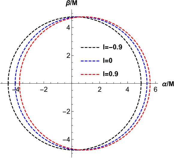
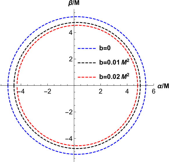
Figure 16: The left panel gives shapes of the shadow for various values of $l$ with $a=0.1M$, $b=0.01M^{2}$, and $\theta=\pi/2$. The right panel gives shapes of the shadow for various values of $b$ with $a=0.1M$ , $l=0.1$, and $\theta=\pi/2$.

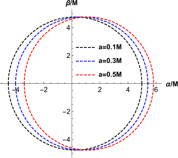
Figure 17: The shapes of the shadow for various values of $a$ with $b=0.01M^{2}$, $l=0.1$, and $\theta=\pi/2$.

From the above plots, we observe that the size of the shadow increases with an increase in $l$, whereas it decreases with an increase in $b$. Besides, if we increase $a$ then the shadow shifts toward the right.

Using the parameters which are introduced by Hioki and Maeda KH , we analyze the deviation from the circularity form $\left(\delta_{s}\right)$ and the size $\left(R_{s}\right)$ of the shadow cast by the black hole.

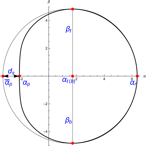
Figure 18: The black hole shadow and reference circle. $ds$ is the distance between the left points of the shadow and the reference circle.

For calculating these parameters, we consider five points $\left(\alpha_{t},\beta_{t}\right),\left(\alpha_{b},\beta_{b}\right),\left(\alpha_{r},0\right)$ $\left(\alpha_{p},0\right)$ and $\left(\bar{\alpha}_{p},0\right)$ which are top, bottom, rightmost, leftmost of the shadow and leftmost of the reference circle respectively. So, we have

$$R_{s}=\frac{\left(\alpha_{t}-\alpha_{r}\right)^{2}+\beta_{t}^{2}}{2\left|\alpha_{t}-\alpha_{r}\right|}$$

and

$$\delta_{s}=\frac{\left|\bar{\alpha}_{p}-\alpha_{p}\right|}{R_{s}}.$$

In the following Fig. We plot $R_{s}$ and $\delta_{s}$ for various scenarios to study how $R_{s}$ and $\delta_{s}$ varies with parameters of the modified theory of gravity.

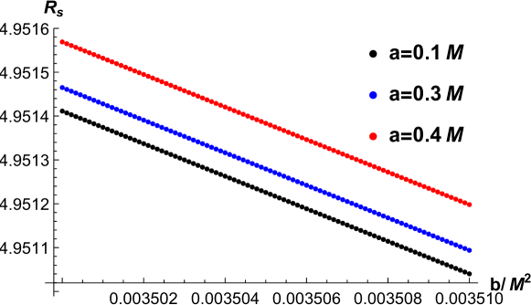
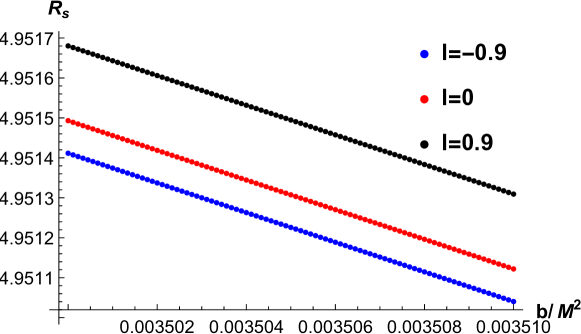
Figure 19: The left panel shows variation of $R_{s}$ for various values of $a$ with $l=-0.2$ and $\theta=\pi/2$, and the right panel shows the variation of $R_{s}$ for various values of $l$ with $a=0.3M$ and $\theta=\pi/2$.

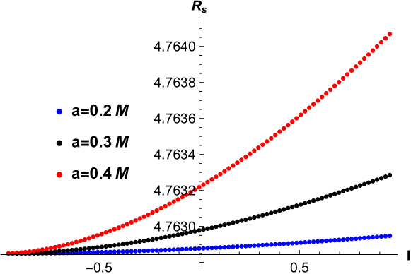
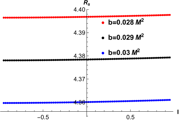
Figure 20: The left panel shows variation of $R_{s}$ for various values of $a$ with $b=0.01M^{2}$ and $\theta=\pi/2$ and the right panel shows the variation of $R_{s}$ for various values of $b$ with $a=0.3M$ and $\theta=\pi/2$.

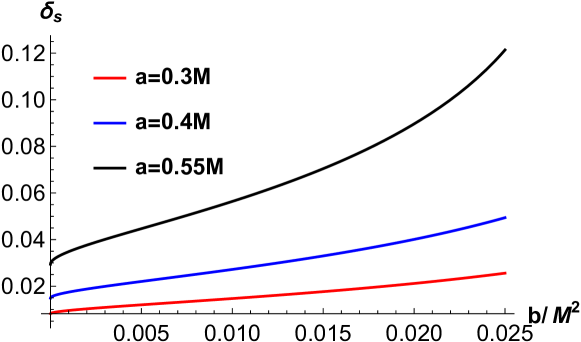
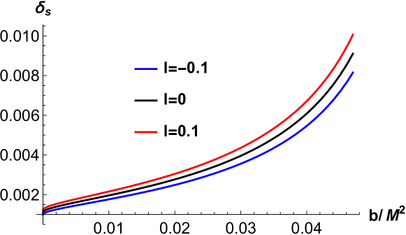
Figure 21: The left panel shows variation of $\delta_{s}$ for various values of $a$ with $l=-0.2$ and $\theta=\pi/2$ and the right panel shows the variation of $\delta_{s}$ for various values of $l$ with $a=0.1M$ and $\theta=\pi/2$.

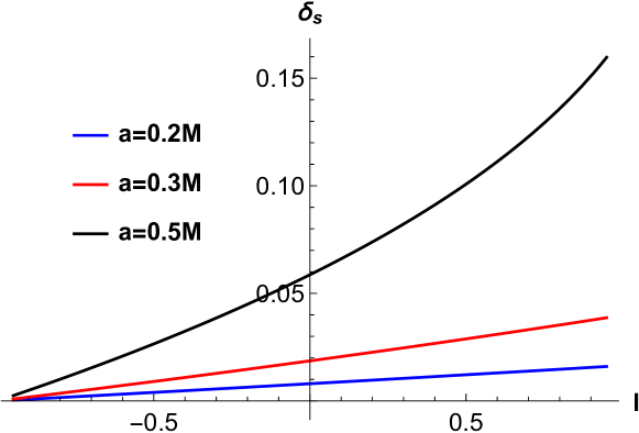
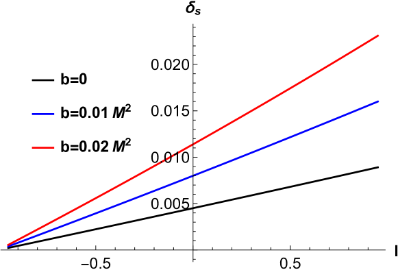
Figure 22: The left panel shows the variation of $\delta_{s}$ for various values of $a$ with $b=.01M^{2}$ and $\theta=\pi/2$ and the right panel one gives the variation of $\delta_{s}$ for various values of $b$ with $a=0.2M$ and $\theta=\pi/2$.

From the above plots we observe that $R_{s}$ decreases with an increase in $b$ for fixed values of $a$ and $l$, whereas for fixed values of $a$ and $b$, it increases with an increase in $l$. On the other hand, $\delta_{s}$ increases with an increase in $l$ for fixed values of $a$ and $b$ as well as with an increase in $b$ for fixed values of $a$ and $l$.

VI Computation of energy emission rate

In this part, we study the possible visibility of the non-commutative Kerr-like black hole through shadow. In the vicinity of limiting constant value, the cross-section of the black hole’s absorption moderates lightly at high energy. We know that a rotating black hole can absorb electromagnetic waves, so the absorbing cross-section for a spherically symmetric black hole is BM

$$\sigma_{lim}=\pi R_{s}^{2}.$$ (65)

Using the above equation the energy emission rate is obtained AA :

$$\frac{d^{2}E}{d\omega dt}=\frac{2\pi^{3}R_{s}^{2}}{e^{\left(\frac{\omega}{T}\right)}-1}\omega^{3},$$ (66)

where $T=\frac{\sqrt{1+\ell}\Delta^{\prime}\left(r_{+}\right)}{4\pi\left[r_{+}^{2}+(1+\ell)a^{2}\right]}$ is the Hawking temperature and $\omega$ the frequency.

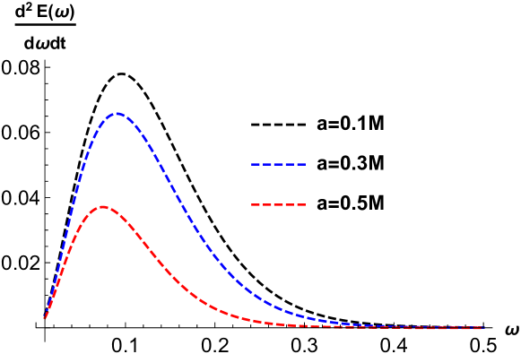
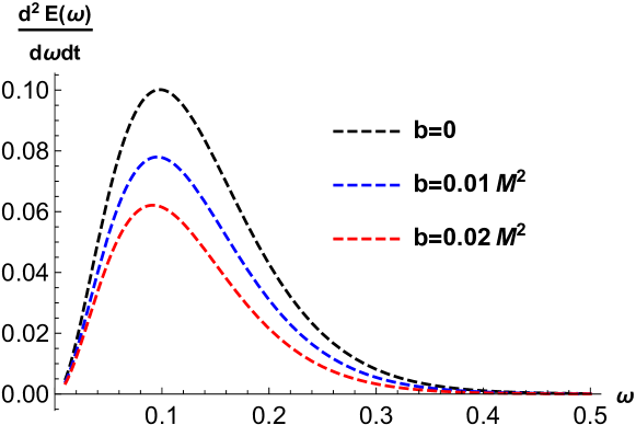
Figure 23: The left panel gives variation of emission rate against $\omega$ for various values of $a$ with $b=.01M^{2}$ and $l=0.3$. The right panel gives variation of emission rate against $\omega$ for various values of $b$ with $a=0.1M$ and $l=0.3$.

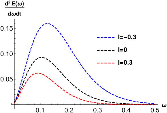
Figure 24: It gives variation of emission rate against $\omega$ for various values of $l$ with $b=0.02M^{2}$ and $a=0.1M$.

In Fig. 17 and 18, we have shown the plots of energy emission rate versus $\omega$ for various cases. It is clear from the plots that the emission rate decreases with an increase in the value of $b$ for any set of fixed values of $a$ and $l$. It also decreases with an increase in $l$, for $a$ and $b$ being fixed, and with an increase in $a$, when $l$ and $b$ remain fixed. Let us now consider the case when some medium is present which is a more natural one.

We now consider the situation when the black hole is veiled with a dispersive medium like plasma and compute the emission rate in this situation. In the presence of plasma, the celestial coordinates are given by OUR

$$\alpha(\xi,\eta;\theta) = -\frac{\xi_{s}\csc\theta}{n},$$

$$\beta(\xi,\eta;\theta) = \frac{\sqrt{\eta+(1+l)a^{2}\cos^{2}\theta-\xi^{2}\cot^{2}\theta-\left(n^{2}-1\right)a^{2}\left(1+l\right)sin^{2}\theta}}{n},$$

where $n=\sqrt{1-\frac{k}{r}}$ ROGERS is the refractive index of the plasma, k being the plasma constant. Using these expressions combined with the expression of emission rate we investigate the variation of rate of emission for various situations.

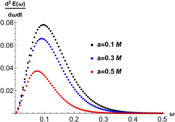
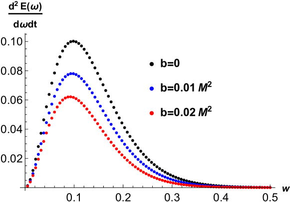
Figure 25: The left panel gives the variation of emission rate against $\omega$ for various values of $a$ with $b=0.01M^{2}$,$k=0.2M$, and $l=0.3$. The right panel gives variation of emission rate against $\omega$ for various values of $b$ with $a=0.1M$, $k=0.2M$, and $l=0.3$.

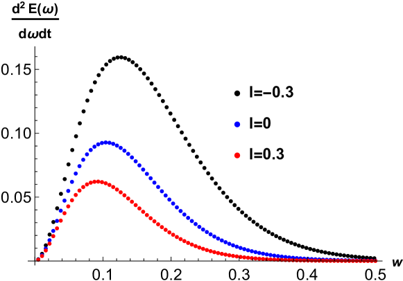
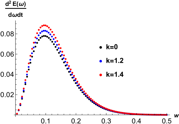
Figure 26: The left panel gives variation of emission rate against $\omega$ for various values of $l$ with $b=.02M^{2}$, $k=0.2M$, and $a=0.1$. The right one gives the variation of emission rate against $\omega$ for various values of $k$ with $a=0.1M$ ,$b=0.01M^{2}$, and $l=0.3$.

Here we observe that the rate of emission increases with the plasma constant $k$ for fixed values of $a,b$, and $l$. The other variations are similar to those which we have seen without plasma, though with reduced values.

VII Constraining from the observed data for $\mathrm{M}87^{*}$

This section is devoted to the constraining of the parameter which are involved in the modified theory. We compare the shadows produced from the numerical calculation by the non-commutative Kerr-like black holes with the observed one for the $\mathrm{M}87^{*}$ black hole. For comparison, we consider the experimentally obtained astronomical data for the deviation from circularity $\Delta\leq 0.10$ and angular diameter $\theta_{d}=42\pm 3\mu as$. The boundary of the shadow is described by the polar coordinate $(R(\phi),\phi)$ with the origin at the center of the shadow $(\alpha_{C},\beta_{C})$ where $\alpha_{C}=\frac{|\alpha_{max}+\alpha_{min}|}{2}$, and $\beta_{C}=0$.

If a point $(\alpha,\beta)$ over the boundary of the image subtends an angle $\phi$ on the $\alpha$ axis at the geometric center, $\left(\alpha_{C},0\right)$, and $R(\phi)$ be the distance between the point $(\alpha,\beta)$ and $\left(\alpha_{C},0\right)$, then the average radius $R_{\text{avg}}$ of the image is given by CBK

$$R_{\text{avg}}^{2}\equiv\frac{1}{2\pi}\int_{0}^{2\pi}d\phi R^{2}(\phi),\\$$ (68)

where $R(\phi)\equiv\sqrt{\left(\alpha(\phi)-\alpha_{C}\right)^{2}+\beta(\phi)^{2}}$, and $\phi=tan^{-1}\frac{\beta(\phi)}{\alpha(\phi)-\alpha_{C}}$.

With the above inputs, the circularity deviation $\Delta C$ is defined by TJDP

$$\Delta C\equiv 2\sqrt{\frac{1}{2\pi}\int_{0}^{2\pi}d\phi\left(R(\phi)-R_{\text{avg }}\right)^{2}}.$$ (69)

We also consider the angular diameter of the shadow which is define by

$$\theta_{d}=\frac{2}{d}\sqrt{\frac{A}{\pi}},$$ (70)

where $A=2\int_{r_{-}}^{r_{+}}\beta d\alpha$ is the area of the shadow and $d=16.8Mpc$ is the distance of $M87^{*}$ from the Earth. These relations will enable us to accomplish a comparison between the theoretical predictions for non-commutative Kerr-like black-hole shadows and the experimental findings of the EHT collaboration. In the figures below the deviation from circularity, $\Delta C$ is shown for non-commutative Kerr-like black holes for inclination angles $\theta=90^{o}$ and $\theta=17^{o}$ respectively.

Figure 27: The left panel is for $l=0.4$, and the right panel is for $b=0.01M^{2}$ where the inclination angle is $90^{o}$. The black solid lines correspond to $\Delta C=0.1$.

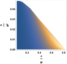
Figure 28: The left panel is for $l=0.4$, and the right one is for $b=0.01M^{2}$ where the inclination angle is $17^{o}$.

In the figures depicted below the angular diameter $\theta_{d}$ is shown for non-commutative Kerr-like black holes for inclination angles $\theta=90^{o}$ and $\theta=17^{o}$ respectively.

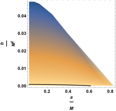
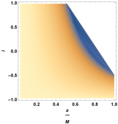
Figure 29: The left panel is for $l=0.4$, and the right panel is for $b=0.01M^{2}$ where the inclination angle is $90^{o}$. The black solid lines correspond to $\theta_{d}=39\mu as$.

     

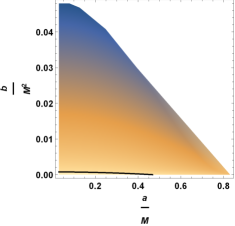
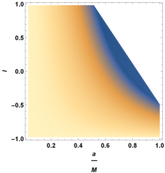
Figure 30: The left panel is for $l=0.4$, and the right panel is for $b=0.01M^{2}$ where the inclination angle is $17^{o}$. The black solid lines correspond to $\theta_{d}=39\mu as$.

From the above plots, we can conclude that the constrain $\Delta C\leq 0.1$ is satisfied for finite parameter space when the inclination angle is $90^{o}$, whereas, when the inclination angle is $17^{o}$, the constrain is satisfied for the entire parameter space. For inclination angles $\theta=90^{o}$ and $\theta=17^{o}$, the constrain $\theta_{d}=42\pm 3\mu$ within $1\sigma$ region is satisfied for finite parameter space. The circular asymmetry in the $M87^{*}$ shadow can also be defined in terms of the axial ratio $D_{X}$ which is the ratio of the major to the minor diameter of the shadow KA1 . It is defined by BCS

$$D_{X}=\frac{\Delta Y}{\Delta X}=\frac{\beta_{t}-\beta_{b}}{\alpha_{r}-\alpha_{p}}.$$ (71)

We should have $1<D_{X}\lesssim 4/3$ in accordance with the EHT observations of $M87^{*}$ KA1 . Note that $D_{X}$ is another way of defining $\Delta C$. Axial ratio of $4:3$ indeed corresponds to a $\Delta C\leq 0.1$ KA1 . In the figures below axial ratio, $D_{X}$ is shown for non-commutative Kerr-like black holes for inclination angles $\theta=90^{o}$ and $\theta=17^{o}$ respectively.

     

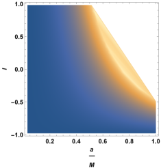
Figure 31: The left panel is for $l=0.4$ and the right panel is for $b=0.01M^{2}$ where the inclination angle is $90^{o}$.

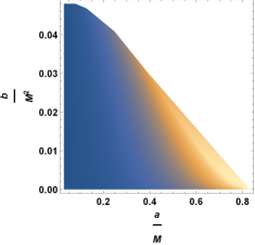
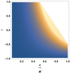
Figure 32: The left panel is for $l=0.4$ and the right panel is for $b=0.01M^{2}$ where the inclination angle is $17^{o}$.

From the plots above we see that the condition $1<D_{X}\lesssim 4/3$ is satisfied for the entire parameter space of non-commutative Kerr-like black holes. Thus non-commutative Kerr-like black holes are remarkably consistent with EHT images of $M87^{*}$. Therefore, we can not rule out non-commutative Kerr-like black holes from the observational data of $M87^{*}$ black hole shadow.

We can have the bound of the parameter $b$ associated with the non-commutativity of the spacetime in a similar way we determined the bound of the parameter $l$ in OUR . By modeling M$87^{*}$ black hole as Kerr black hole, the author of the article RODRIGO obtained a lower limit of $a$ for the M$87^{*}$ black hole. Bringing this result under consideration in OUR we put the interval of interest for $a$ as $[0.50M,0.99M]$, and using the experimental constraints $\Delta C\leq 0.10$ and $\theta_{d}=42\pm 3\mu as$ with the information $a\in[0.50M,0.99M]$, we observed that $l\in(-1,0.621031]$. In a similar way taking into account the bounds $a\in[0.50M,0.99M]$ and $l\in(-1,0.621031]$ and the experimental constraints $\Delta C\leq 0.1$ and $\theta_{d}=39\pm 3\mu as$, we get a bound on the parameter $b$ which is linked with the non-commutativity of spacetime. We find that the parameter $b\in[0,0.000505973M^{2}]$. It is intriguing to have an upper bound of $b$ which is found out to be $0.000505973M^{2}$. To the best of our knowledge, the bound of the parameter $b$ from the shadow of the astronomical black hol has not yet been reported so far.

VIII Summary and Conclusion

In this work, we have developed a framework where quantum correction due to the Lorentz violation and noncommutativity of spacetime have been taken into account on the same footing. The spacetime background renders a non-commutative Kerr-like LV black hole. We have extensively studied different aspects of the non-commutative and LV Kerr-like black hole. The spin, the mass, the LV parameter, and the non-commutative parameter involved in it determine the gravitational field of this black hole. First of all, we study geometry in detail concerning its horizon structure and ergosphere.

The study of the two important optical phenomena in the vicinity of this black hole was our main objective in this article. In this respect, we first have consider the superradiance phenomena and find that it crucially depends on the parameter $l$ and $b$ apart from itsdependence on $a$ which is licked with the spin of the black hole. The superradiance process enhances with the decrease in the value of the LV parameters and it diminishes when the increase in value of the LV parameter. We also observe that with the increase in the value of the parameter $b$ the superradiance process gets diminished. However, with the increase in the value of $a$ the superradiance process increases.

Next, we have brought into our investigation the effect of Lorentz violating parameter $l$ and non-commutative parameter $b$ on the size of the black hole shadow. We have observed that the size of the black hole shadow increases with an increase in the value of the parameter $l$, and it decreases with an increase in the value of the parameter $b$. Thus, it can be safely concluded that Lorentz violation and non-commutativity, both, have significant impacts on black hole shadow.

We have also studied emission rates in the presence of plasma and also in the absence of it to make a comparison between these two cases. Our study shows that although the emission rate changes with the variation of the plasma parameter, the nature of the emission curves remains unaltered in both cases: in the presence and in the absence of plasma. These results have clearly established the influence of the LV parameter and non-commutative parameter on emission rate. Besides, it being a generic study, we can also obtain the results for Kerr and Kerr-like black holes with suitable limits

We have made an attempt to constrain parameters in our modified theories using the observations of EHT collaboration. For inclination angle $\theta=90^{o}$, the deviation from circularity $\Delta C\leq 0.1$ and angular diameter $\theta_{d}=42\pm 3\mu$as within $1\sigma$ region are satisfied for finite parameter space $(\frac{b}{M^{2}}-\frac{a}{M})$ and $(l-\frac{a}{M})$. For inclination angle $\theta=17^{o}$, the circularity deviation $\Delta C\leq 0.1$ is satisfied for entire parameter space $(\frac{b}{M^{2}}-\frac{a}{M})$ and $(l-\frac{a}{M})$. The angular diameter $\theta_{d}=42\pm 3\mu$ as within $1\sigma$ is satisfied for finite parameter space $(\frac{b}{M^{2}}-\frac{a}{M})$ and $(l-\frac{a}{M})$. The axis ratio $D_{X}$ satisfies the constraint $1<D_{X}\lesssim 4/3$ for the entire parameter space at both the inclination angles $\theta=90^{o}$ as well as $\theta=17^{o}$. Therefore our study enables to establish the fact that non-commutative Kerr-like black holes are remarkably consistent with EHT images of $M87^{*}$. It demands that ruling out non-commutative Kerr-like black holes from the observational data of black hole shadow would be illogical. Thus non-commutative Kerr-like black hole may be considered as a suitable candidate for the astrophysical black hole. It has also been shown that the possible upper bound of $b$ which is associated with the non-commutativity is $0.000505973M^{2}$. It is intriguing and indeed a novel way to constrain the parameter associated with the non-commutativity from the shadow of an astronomical black hole.

Till now we do not have any available data to constrain the parameter $l$ and $b$ from the superradiance effect and from the energy emission process. So the parameter con not be constrained by knowledge of the superradiance phenomena and the energy emission process. We have made all the plots for the superradiance and the energy emission process maintaining the constraint obtained from the EHT data concerning the shadow of the $M87^{*}$.

References

- (1) Y. B. Zel’dovich Pis’ma Zh. Eksp. Teor. Fiz. 14 (1971) 270 [JETP Lett. 14, 180 (1971)].
- (2) Y. B. Zel’dovich Zh. Eksp. Teor. Fiz 62 (1972) 2076 [Sov.Phys. JETP 35, 1085 (1972)].
- (3) R. Brito, V. Cardoso, P. Pani: Lecture Notes in Physics (2nd edition) 971 (2020)
- (4) S. Hawking, Commun.Math.Phys. 43 (1975) 199
- (5) A. Arvanitaki, S. Dimopoulos, S. Dubovsky, N. Kaloper, and J. March-Russell, Phys.Rev. D81(2010) 123530,
- (6) A. Arvanitaki, S. Dubovsky, Phys.Rev. D83 (2011) 044026,
- (7) P. Pani, V. Cardoso, L. Gualtieri, E. Berti, A. Ishibashi, Phys.Rev.Lett. 109 (2012) 131102,
- (8) R. Brito, V. Cardoso, P. Pani, Phys. Rev. D88 (2013) 023514
- (9) C. A. R. Herdeiro and E. Radu, Phys.Rev.Lett. 112 (2014) 221101,
- (10) V. Cardoso and O. J. Dias, Phys.Rev. D70 (2004) 084011,
- (11) O. J. Dias, P. Figueras, S. Minwalla, P. Mitra, R. Monteiro, et al. JHEP 1208(2012) 117
- (12) O. J. Dias, G. T. Horowitz, and J. E. Santos, JHEP 1107 (2011) 115,
- (13) M. Shibata and H. Yoshino, Phys. Rev. D81 (2010) 104035,
- (14) J. L. Synge: MNRAS 131 463 1966.
- (15) J. P. Luminet: Astronmy & Astrophysics, 75, 228 (1979).
- (16) J. M. Bardeen, W. H. Press, S. A. Teukolsky: Astro-phys. J. 178, 347 (1972).
- (17) S. Chandrasekhar, The Mathematical Theory of Black Holes, Oxford University Press, New York, (1992)
- (18) K. Hioki and K. I. Maeda: Phys. Rev. D80, 024042 (2009).
- (19) T. Johannsen, D. Psaltis: Astrophys. J. 718, 446 (2010).
- (20) K. Akiyama et al.: Astrophys. J. 875, L1 (2019).
- (21) K. Akiyama et al.: Astrophys. J. 875, L2 (2019).
- (22) K. Akiyama et al.: Astrophys. J. 875, L3 (2019).
- (23) K. Akiyama et al.: Astrophys. J. 875, L4 (2019).
- (24) K. Akiyama et al.: Astrophys. J. 875, L5 (2019).
- (25) K. Akiyama et al.: Astrophys. J. 875, L6 (2019).
- (26) F. Atamurotov, B. Ahmedov, A. Abdujabbarov: Phys. Rev. D92, 084005 (2015).
- (27) V. Perlick, O. Y. Tsupko: Phys. Rev. D 95, 104003 (2017).
- (28) Shao-Wen Wei, Yu-Xiao Liu: JCAP 11, 063 (2013).
- (29) G. Z. Babar, A. Z. Babar, F. Atamurotov: Euro. Phys. Jour. C80, 761 (2020).
- (30) S. Dastan, R. Saffari, S. Soroushfar: arXiv:1610.09477
- (31) D. Mattingly: Living Rev. Rel. 8, 5 (2005)
- (32) K. Bakke H. Belich: Eur. Phys. J. Plus 129: 147 (2014).
- (33) V. A. Kostelecky, C. D. Lane: Journal of Mathematical Physics 40, 6245 (1999).
- (34) T. J. Yoder and G. S. Adkins: Phys. Rev. D 86, 116005 (2012).
- (35) R. Lehnert: Phys. Rev. D 68, 085003 (2003).
- (36) O. G. Kharlanov, V. Ch. Zhukovsky: J. Math. Phys. 48, 092302 (2007).
- (37) V. A. Kostelecky and M. Mewes: Phys. Rev. Lett. 87, 251304 (2001).
- (38) V. A. Kostelecky and M. Mewes: Phys. Rev. D 66, 056005 (2002).
- (39) V. A. Kostelecky and M. Mewes: Phys. Rev. Lett. 97, 140401 (2006).
- (40) V. A. Kostelecky and M. Mewes: Phys. Rev. Lett. 87, 251304 (2001).
- (41) S. Carroll, G.B. Field, and R. Jackiw: Phys. Rev. D 41, 1231 (1990).
- (42) C. Adam and F. R. Klinkhamer: Nucl. Phys. B 607, 247 (2001).
- (43) W. F. Chen and G. Kunstatter: Phys. Rev. D 62, 105029 (2000).
- (44) C. D. Carone, M. Sher, M. Vanderhaeghen: Phys. Rev. D74, 077901 (2006).
- (45) F.R. Klinkhamer and M. Schreck: Nucl. Phys. B848, 90 (2011).
- (46) M. Schreck: Phys. Rev. D86, 065038 (2012).
- (47) M. A. Hohensee, R. Lehnert, D. F. Phillips, R. L. Walsworth: Phys. Rev. D80, 036010 (2009).
- (48) B. Altschul and V. A. Kostelecky: Phys. Lett. B628, 106.
- (49) R. Bluhm, N. L. Gagne, R. Potting, A. Vrublevskis: Phys. Rev. D 77, 125007 (2008).
- (50) R. Bluhm, V. Alan Kostelecky: Phys. Rev. D71, 065008 (2005).
- (51) R. V. Maluf, V. Santos, W. T. Cruz, C. A. S. Almeida: Phys. Rev. D88, 025005 (2013).
- (52) R.V. Maluf, C.A.S. Almeida, R. Casana, M.M. Ferreira, Jr.: Phys. Rev. D 90 025007 (2014)
- (53) Q. G. Bailey and V. A. Kostelecky: Phys. Rev. D74, 045001 (2006).
- (54) V. A. Kostelecky, S. Samuel: Phys. Rev. D39 683 (1989).
- (55) V. A. Kostelecky, S. Samuel: Phys. Rev. Lett. 63, 224 (1989).
- (56) V. A. Kostelecky, S. Samuel: Phys. Rev. D 40, 1886 (1989).
- (57) D. Colladay and V. A. Kostelecky: Phys. Rev. D 55, 6760 (1997)
- (58) D. Colladay, V.A. Kostelecky: Phys. Rev. D 55, 6760 (1997); Phys. Rev. D 58, 116002 (1998)
- (59) V. A. Kostelecky: Phys. Rev. D69, 105009 (2004)
- (60) D. Colladay, V.A. Kostelecky: Phys. Rev. D 55, 6760 (1997).
- (61) D. Colladay, V.A. Kostelecky: Phys. Rev. D 58, 116002 (1998)
- (62) C. Ding, C. Lui, R. Casana: A. Cavalcante: Eur. Phys. J. C80 178 2020.
- (63) R. Casana and A. Cavalcante: Phys. Rev. D 97, 104001 (2018).
- (64) S. K. Jha, A. Rahaman: Eur. Phys. J C81 345 (2021)
- (65) R. J. Szabo: Phys. Rept. 378 207 (2003)
- (66) S. M. Carroll, J. A. Harvey, V. A. Kostelecky, C. D. Lane, T. Okamoto: Phys. Rev. Lett. 87, 141601 (2001)
- (67) Jian Jing, Ling-Bao Kong, Qing Wang, Shi-Hai Dong: Phys.Lett. B808 135660 (2020)
- (68) S. Bhattacharyya, S. Gangopadhyay, A. Saha: Class.Quant.Grav. 36 055006 (2019)
- (69) R. Fresneda, D.M. Gitman, A. E. Shabad: Phys.Rev. D91 085005 (2015)
- (70) C. B Luo, F. Y. Hou, Z. F Cui, X. J. Liu, H. S. Zong: Phys.Rev. D91 036009 (2015)
- (71) P. Nicolini: Int. J. Mod. Phys. A 24, 1229 (2009)
- (72) P. Aschieri, C. Blohmann, M. Dimitrijevic, F. Meyer, P. Schupp, J. Wess: Class. Quant. Grav. 22, 3511 (2005)
- (73) P. Aschieri, M. Dimitrijevic, F. Meyer, J. Wess: Class. Quant. Grav. 23, 1883 (2006)
- (74) S. Meljanac, A. Samsarov, M. Stojic, K. S. Gupta: Eur. Phys. J. C 53, 295 (2008)
- (75) E. Harikumar, T. Juric and S. Meljanac: Phys. Rev. D 86, 045002 (2012)
- (76) P. Nicolini, A. Smailagic, E. Spallucci: Phys. Lett. B 632, 547-551 (2006).
- (77) K. Nozari and S. H. Mehdipour: Class. Quant. Grav. 25, 175015 (2008)
- (78) R. Casana, A. Cavalcante, F. P. Poulis, E. B. Santos: Phys. Rev. D 97, 104001 (2018)
- (79) A. H. Klotz, Gen. Gel. Grav. 14, 727 (1982)
- (80) W. Kim, E. J. Son, M. Yoon: JHEP 0804, 042 (2008)
- (81) K. Nozari, S. H. Mehdipour: JHEP 0903, 061 (2009)
- (82) R. Banerjee, B. R. Majhi and S. Samanta: Phys. Rev. D77, 124035 (2008)
- (83) S. H. Mehdipour: Commun. Theor. Phys. 52, 865 (2009)
- (84) S. H. Mehdipour: Phys. Rev. D 81, 124049 (2010)
- (85) Y. G. Miao, Z. Xue and S. J. Zhang: Gen. Rel. Grav. 44, 555 (2012)
- (86) K. Nozari and S. Islamzadeh: Astrophys. Space Sci. 347, 299
- (87) A. Ovgun and K. Jusufi: Eur. Phys. J. Plus 131 177 (2016)
- (88) K. S. Gupta, T. Juric, A. Samsarov: JHEP 1706, 107 (2017)
- (89) J. Liang and B. Liu: Eur. Phys. Lett. 100, 30001 (2012)
- (90) P. Nicolini, Int. J. Mod. Phys. A 24 (2009) 1229
- (91) R.J. Szabo, Class. Quantum Gravity 23 (2006) R199
- (92) A. Smailagic, E. Spallucci, J. Phys. A 36 (2003) L467
- (93) A. Smailagic, E. Spallucci, J. Phys. A 36 (2003) L517
- (94) P. Nicolini, A. Smailagic, E. Spallucci, Phys. Lett. B 632 (2006) 547
- (95) K. Nozari, S.H. Mehdipour, Class. Quantum Gravity 25 (2008) 175015
- (96) S. K. Jh, H. Barman, A. Rahaman: 04 036 (2021)
- (97) M. A. Anacleto, F. A. Brito, J. A. V. Campos, E. Passos: Phys. Lett. B803, 135334 (2020)
- (98) R. Penrose: Riv. Nuovo Cim. 1, 252 (1969).
- (99) B. Mashhoon: Phys. Rev. D7, 2807 (1973)
- (100) A. Abdujabbarov, M. Amir, B. Ahmedov, S. G. Ghosh: Phys. Rev. D93, 104004 (2016)
- (101) S. K. Jha, S. Aziz, A. Rahaman: to appear in Eur. Phys. J C, arXiv:2103.17021
- (102) A. Rogers: MNRAS, 451 17 2015
- (103) C. Bambi, K. Freese, S. Vagnozzi, L. Visinelli: Phys.Rev.D100 044057 (2019).
- (104) I. Banerjee, S. Chakraborty, S. Sengupta: Phys. Rev. D101, 041301 (2020).
- (105) R. Nemmen: Astrophys J. Letts L26 880 (2019)
- (106) S. Kanzi, I. Sakalli: EPJC Doi:10.1140/epjc/s10052-022-10044-2
- (107) S. Hod, Phys. Lett. B 708 (2012) 320 [arXiv:1205.1872 [gr-qc]].
- (108) A. A. Starobinsky, Zh. Eksp. Teor. Fiz. 64, 48 (1973) [Sov.Phys. JETP 37, 28 ( 1973)]
- (109) A. A. Starobinsky and S. M. Churilov: Zh. Eksp. Teor. Fiz. 65, 3 (1973) [Sov. Phys. JETP 38, 1 (1973)].
- (110) S. A. Teukolsky, W. H. Press: Astrophys. J. 193 443 (1974)
- (111) D. N. Page: Phys. Rev. D13 198 (1976)
- (112) Ran Li: Phys. Lett. B714 337 (2012)
- (113) V. B. Bezerra , H. S. Vieira, A. A. Costa: Class.Quantum Grav. 31 045003 (2014)
- (114) G. V. Kraniotis: Class.Quant.Grav. 33 225011 (2016)
- (115) M. Khodadi: Phys.Rev. D103, 064051 (2021)
- (116) R. Brito, V. Cardoso, P. Pani: Lecture Notes in Physics (2nd edition) 971 (2020)