prose: A Python framework for modular astronomical images processing

Abstract

To reduce and analyze astronomical images, astronomers can rely on a wide range of libraries providing low-level implementations of legacy algorithms. However, combining these routines into robust and functional pipelines requires a major effort which often ends up in instrument-specific and poorly maintainable tools, yielding products that suffer from a low-level of reproducibility and portability. In this context, we present prose, a Python framework to build modular and maintainable image processing pipelines. Built for astronomy, it is instrument-agnostic and allows the construction of pipelines using a wide range of building blocks, pre-implemented or user-defined. With this architecture, our package provides basic tools to deal with common tasks such as automatic reduction and photometric extraction. To demonstrate its potential, we use its default photometric pipeline to process 26 TESS candidates follow-up observations and compare their products to the ones obtained with AstroImageJ, the reference software for such endeavors. We show that prose produces light curves with lower white and red noise while requiring less user interactions and offering richer functionalities for reporting.

Introduction

When an astronomical observation is completed, one has to process its raw products into a desired output. Observatories and survey-specific pipelines are sometimes available but general or custom software are often required, offering higher flexibility and control. These tools and their development benefit from legacy and modern algorithms, implemented into community-maintained libraries (like IRAF (Tody, 1986) or astropy (Astropy Collaboration et al., 2013, 2018)). However developing a custom option requires time and effort. Indeed, once the algorithms are selected, their implementations must be assembled into a code ingesting raw FITS images. To reach an optimized output, a fine-tuning of this code is often required, from its individual processing components up to the complete pipeline, including complex I/O operations and architecture choices. In its final version, the software is generally frozen and maintained when it breaks. These tools, whether custom or third-party, seldom provide a complete analysis framework such that their end products are exploited into scripting languages such as Julia or Python.

We propose an alternative for that. Pipelines can generally be described as a sequence of individual data-processing units. These processing units (hereafter called Blocks) are fundamentally common from one pipeline to another. They complete independent tasks using algorithms widely used by the whole community. Hence, in a framework where Blocks are all inter-compatible, one would only have to focus on which algorithms to use and assemble Blocks into a modular pipeline, with no need for software architecture considerations.

In this paper, we present prose, a Python package acting as a framework to build modular pipelines for astronomy, allowing rapid iterations toward specific needs and rich scientific products. Its architecture allows the creation of inter-compatible Blocks, many being pre-implemented and available in the initial package. Developed in the context of transiting exoplanet observations, it contains tools specific to high-precision point-source photometry. However, the aim of prose is to be versatile and to adapt to a variety of astronomical datasets.

In section 1, we present the key concepts behind prose, as well as some of the pre-implemented blocks it features. In section 2, we present a pipeline, developed with prose, built to reduce raw astronomical images and perform high-precision differential photometry. To remain fast on domestic computers, this pipeline relies on two algorithms: a fast registration technique based on Lang et al. (2010) and a neural network based centroiding method, both described in details in section 2. In xsection 3, we assess our built-in photometric pipeline’s performances by processing 26 TESS candidates follow-up observations, mainly from the TRAPPIST-South telescope (Jehin et al., 2011; Gillon et al., 2011), and compare their final light curves to those obtained with AstroImageJ (AIJ, Collins et al. 2017), the main software used by the TESS Follow-up Observing Program working group (TFOP) to process ground-based transit follow-up observations.

1 prose

1.1 Images, Blocks and Sequences

A pipeline, strictly speaking, is a series of connected tubes running a fluid. In the scientific literature, the word refers to processing pipelines in which data are flowing, going through processing units as in tubes. Image processing algorithms are implemented as standalone codes which are easy to run on a single image. However, assembling multiple low-level codes, successively ran on a set of images requires a complete architecture to be built and tested. The final result is often monolithic, far from where we take the word pipeline from. Of course, the flexibility offered by lower-level codes is essential but we believe generalizing the approach of building pipelines for astronomical image processing comes with great advantages.

prose contains the structure for such a modular concept to work by providing three key objects: Images, Blocks and Sequences. An Image encapsulates the data and metadata of an exposure frame. A Block is a single processing unit that acts on an Image. Finally, a Sequence is a series of Blocks. A pipeline is then an assembly of Sequences.

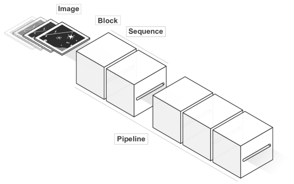
Figure 1: Illustration of prose key objects

1.2 Blocks

With this architecture, one can focus on designing robust and reusable Blocks, well tested and independently maintainable. To do that, prose comes with pre-implemented Blocks featuring common state-of-the-art algorithms, some being listed in Table 1. In this table, the symbol * refers to Blocks using implementations from other sources, like PhotutilsAperturePhotometry which relies on the aperture photometry implementation of photutils, or SEDetection using SExtractor (Bertin & Arnouts, 1996) through the sep Python package.

Calibration and utils	Detection	PSF estimate
Calibration	DAOFindStars*	FastGaussian
Flip	IrafFindStars*	Gaussian2D
Trim	SEDetection*	Moffat2D
MedianStack	SegementedPeaks
Video
Alignment and registration	Photometry
XYShift	PhotutilsAperturePhotometry*
Twirl	SEAperturePhotometry*
AffineTransform
BalletCentroid

Table 1: List of some base Blocks currently included in prose. * refers to Blocks whose implementation is mainly coming from other packages or libraries.

Describing all base Blocks of prose is beyond the scope of this paper, and we refer the interested reader to the prose online documentation.

1.3 Telescope

Blocks are likely to use Image characteristics to complete their tasks. In the case of FITS images, this information is located in their headers, whose definition may differ between observatories. To deal with this variety, prose provides a Telescope object containing a semantic dictionary of keywords used to retrieve physical quantities from image headers. Once a new Telescope is declared, its dictionary is saved and used whenever its name appears, filling the appropriate Image metadata. This mechanism, also found in general reduction tools like AIJ, allows prose to be instrument-agnostic but is only suited to single extension FITS products containing simple headers. Images from the Vatican Advanced Technology Telescope 4K camera (VATT4k), for example, are taken by two amplifiers, leading to FITS images spread over two extensions. Each of these extensions contains data as well as useful header information, while more general characteristics can be found in a separate primary header. To allow such images to be combined and processed, prose allows custom Image loaders to be developed (which in the case of the VATT4k images, for example, consists in 5 lines of Python code).

1.4 A simple example

Most of prose Blocks use state-of-the-art methods and libraries. Its novelty stands in its object-oriented structure, allowing for powerful abstraction in implementing custom pipelines. In this section, we present a simple example: a pipeline to characterize the effective point-spread-function (PSF) of images taken during a full night of observation. For every image, the pipeline starts with bias, dark and flat calibration (Howell, 2006, section 4.5). Then, bright stars are detected to build an effective PSF cutout and characterized using a specific PSF model. Here, we will use a 2D Moffat profile (Moffat, 1969) and only focus on its full width at half maximum (FWHM). Finally, images are stacked and a movie of the night is generated for further vetting.

The Python code to build such a pipeline with prose is shown in Figure 2, where Blocks have been assembled into a single Sequence to perform each task.

⬇

1 from prose import Sequence, FitsManager

2 from prose import blocks

3

4 fm = FitsManager("images-folder")

5

6 sequence = Sequence([

7 blocks.Calibration(**fm.calibs),

8 blocks.DAOFindStars(n=100),

9 blocks.Moffat2D(),

10 blocks.Get("fwhm"),

11 blocks.Video("video.gif"),

12 blocks.Stack(),

13 ], fm.images)

14

15 sequence.run()

Figure 2: (Left) Python code of the pipeline described in subsection 1.4, performing the characterization of images effective PSF over a full night of observation. (Right) resulting stack image and PSF model of the observation produced using products directly accessible from the sequence object. This example is made from 742 10s exposure images taken by the TRAPPIST-South telescope on December 14, 2018.

In this pipeline, a wide range of stellar profiles or detection techniques may be experimented with through the use of different Blocks. The prose online documentation provides many more examples as well as the description of several convenient tools, such as the FitsManager object, allowing to deal with highly disorganized FITS folders by using their header information.

2 Base photometric pipeline

2.1 Principle

Using the structure described in section 1, prose features a standard photometric reduction pipeline which requires minimal user input and can be decomposed in four Sequences: Sequence 1 consists in detecting the $n$ brightest stars from a single image taken from the full observation. These $n$ positions are stored and will act as a reference to align all other frames on. During Sequence 2, each image goes through bias, dark, and flat calibration (Howell, 2006, section 4.5). On each of them, we detect the $n$ brightest stars and compare their positions to the set of reference ones. Image misalignment from the reference can reasonably be approximated by an affine transformation that we compute using the method described in Lang et al. (2010) (see subsection 2.3). We then form a stack image out of transformed frames using bi-linear interpolation but we only save the untransformed calibrated frames as to make the photometry on non-interpolated images. In sequence 3, we detect stars in the stack image (500 by default) and characterize their profile to aid in scaling apertures radii in the next sequence. Finally, sequence 4 consists in extracting the detected stars’ fluxes using circular aperture photometry (Stetson, 1987) on calibrated frames. Although they are not aligned, stars positions in these images can be computed from the ones detected in the stack image (aligned to the reference image) by applying the inverse transformation matrix previously computed and stored for each exposure. As the detector sampling might introduce an error on these local coordinates, a centroiding algorithm is finally used (see subsection 2.4) to properly center each aperture on every image from which the fluxes are finally extracted. Table 2 shows the four sequences described above: 1. Reference stars detection to align other images on; 2. Calibration, alignment and stacking of every frame; 3. A global star detection on the stack image; and 4. Aperture photometry on each calibrated frame refined by a centroiding algorithm.

The inverse transformation we rely on in our pipeline is indirectly adopted by many reduction tools (such as Collins et al. 2017) where stars positions are set in a World Coordinate System (WCS, Wells & Greisen 1979). Indeed, some of them require all frames to be plate-solved which is generally done using Lang et al. (2010) through the astrometry.net service. While we leverage the same asterisms matching algorithm (see subsection 2.3), we do not relate our transformation to a WCS and allow raw images to be processed in a standalone and efficient way. We note that AIJ do not require plate-solved images and rely on a centroiding algorithm to reposition apertures on drifting stars. However, this strategy is only valid for images whose translation is lower than the aperture’s radius, which is what motivated the addition of a complete registration algorithm in our pipeline. We also note that the apertures used in the aperture photometry task are scaled based on an analytical fit to the effective PSF of the detector, hence assuming a known PSF model. In its current version, prose features Blocks to account for Gaussian and Moffat profiles (Moffat (1969), see subsection 2.4), which are only suited to focused PSF. For this reason, follow-up work will include the development of Blocks to properly treat unfocused profiles (which are often ring-shaped and currently depart from default settings).

The products we obtain by running the pipeline can be accessed within a Python instance and saved for later use in a .phot file including the stacked frame of the observation, as well as the positions and fluxes of detected stars at all times and apertures given with their uncertainties. A variety of time-series recorded by individual Blocks are saved as well, such as the mean FWHM of the effective PSF, airmass, background level or frame misalignment, overall essential to model the extent of systematic signals in the measured fluxes.

1. Reference stars detection (on the reference image)
Calibration	Bias, dark, and flat calibration
Trim	Border trimming
SegmentedPeaks	Detection of a reference set of stars
2. Calibration, alignment and stacking (on all raw images)
Calibration	Bias, dark and flat calibration
Trim	Border trimming
Flip	Image flip according to the reference
SegmentedPeaks	Fast detection of stars positions
Moffat2D	Effective PSF characterization
Twirl	Computing affine transformation
SaveReduced	Saving calibrated image
AffineTransform	Applying affine transformation
Stack	Adding transformed image to stack
Video	Adding transformed image to video
3. Stars detection (on the stack image)
DAOFindStars	Stars detection
Moffat2D	Stacked effective PSF characterization
4. Aperture photometry (on calibrated images)
AffineTransform	Applying inverse affine transformation
BalletCentroid	Refining stars centroid positions
PhotutilsAperturePhotometry	Aperture photometry
XArray	Saving fluxes and other measurements.

Table 2: The four sequences of prose default photometric pipeline

2.2 Differential photometry

During the reduction, visible stars are automatically detected for every frame and aperture photometry is performed over a range of 40 apertures, yielding ideal measurements to leverage the power of ensemble differential photometry. For that purpose, prose implements a pure Python version of the algorithm described in Broeg et al. (2005). This algorithm consists in building an artificial comparison star using the weighted sum of all available stars in the field. Appropriate weights are iteratively found as to minimize variance over all differential light curves. Doing so, higher weights are given to stars displaying lower variability and higher signal-to-noise ratio (SNR), more likely to feature systematic signals shared among all sources. Finally, the best aperture is chosen as the one minimizing the white noise of the target’s light curve, estimated with the median standard deviation of points within 5 minutes bins. As all products are saved within a .phot file, light curves for different apertures can later be explored and the best one selected manually.

Our photometric pipeline relies on a strategy which consists in registering all images before refining stars centroids to perform aperture photometry. If processing time is a concern, general registration and centroiding algorithms can be a problem. To keep it fast on domestic computers, we rely on two methods, integrated into Blocks, yielding fast and robust estimates: Twirl which computes the affine transformation between two sets of stars using the method from Lang et al. (2010), and BalletCentroid, a novel centroiding algorithm based on the convolutional neural network presented in Herbel et al. (2018). We present these methods in the next sections.

2.3 Twirl: stars registration

Stars registration is a common need in astronomy. Given two sets of stars positions, it consists in identifying pairs of coordinates corresponding to unique objects, but observed from different referential, hence giving an absolute reference in the sky. To do that, many algorithms, as well as humans, birds, and seals (Foster et al., 2018), use asterisms: shapes produced by stars arrangements, like constellations, recognizable in the sky. In our case, we will use the method of Lang et al. (2010) standing at the core of the widely adopted astrometric calibration service astrometry.net. While it produces robust astrometric solutions, it requires a cross-match to reference stars catalogs that we want to avoid in our pipeline. Hence, our implementation does not provide a complete WCS solution but a transformation matrix allowing stars to be registered to a common frame.

The algorithm starts by computing four-points asterisms, translated into unique hash codes consisting in four numbers as described in Figure 3. These codes have the advantage of being invariant over any affine transformation. Then, starting with two sets of coordinates, set 1 and set 2, their hash codes can be produced and matched to find the transformation they originate from. We produce unique hash codes the same way as Lang et al. (2010) but we use a simpler matching strategy. We organize the hash codes into a kd-tree structure (as in Lang et al. (2010) but using an implementation from scipy.spatial.KDTree) which allows for fast nearest-neighbor lookup. For all asterims in set 1, we retrieve the closest asterism from set 2, compute its corresponding transformation, apply it to set 1 and count the number of stars that can be cross-matched between the two sets (given a tolerance). Finally, we keep the transformation maximizing the number of matched stars.

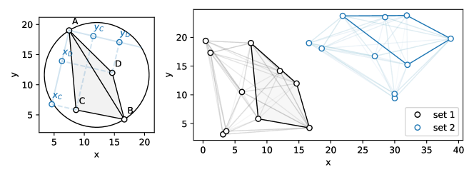
Figure 3: Demonstration of the four-points asterisms used in Twirl. The left figure is reproduced from Lang et al. (2010) and shows how a unique hash code $(x_{C},y_{C},x_{D},y_{D})$ is formed from four points coordinates: by taking the relative positions of two of the coordinates (C, D) with respect to the outermost ones (A and B). The right plot shows the matching of this same asterism with one from another set.

Our method is implemented in the Twirl Block which, given reference coordinates, computes and stores the affine transformation matrix from one set to the reference one. We make its Python implementation (separated from prose) publicly available in the twirl repository .

2.4 ballet: Fast centroiding

Stars positions being computed, as well as their alignment to a common reference, the caveat of our strategy is to rely on a centroiding algorithm to refine their centroids on every frame, which can be CPU intensive and lead to variable results depending on the method used. Inspired by Herbel et al. (2018), we trained a deep Convolutional Neural Network (CNN) to predict accurate centroid positions out of normalized stars cutouts.

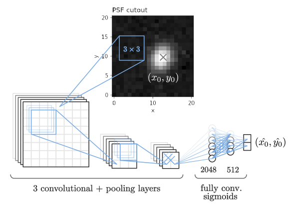
Figure 4: Neural network architecture

The architecture of our neural network is shown in Figure 4 and consists in 3 ReLu-activated convolutional layers of sizes 64, 128 and 256, each followed by a pooling layer downsampling their outputs by a factor 2. The 1028 resulting weights serve as inputs to 2 sigmoid-activated fully connected layers, finally leading to the centroid $(x,y)$ coordinates. This CNN was implemented with the tensorflow package, and trained using the Adam stochastic gradient descent algorithm (Kingma & Ba 2017) on a Huber loss function (Huber, 1964). The training samples consisted in $2\cdot 10^{5}$ simulated Moffat profiles Moffat (1969) expressed as:

$$F(x,y)=b+\frac{1}{\left(1+\frac{dx^{2}}{\sigma_{x}^{2}}+\frac{dy^{2}}{\sigma_{y}^{2}}\right)^{\beta}}$$ (1)

$$\text{where}\begin{cases}dx=(x-x_{0})\cos{\theta}+(y-y_{0})\sin{\theta}\\ dy=-(x-x_{0})\sin{\theta}+(y-y_{0})\cos{\theta}\\ \end{cases}$$ (3)

with $(x_{0},y_{0})$ the centroid position, $(\sigma_{x},\sigma_{y})$ the standard deviation of the point-spread-function (PSF) in the $x$ and $y$-axis, $\theta$ its relative angle with respect to the $x$-axis, $\beta$ the concentration of the Moffat profile and $b$ its relative background. To train the model, these parameters were randomly drawn from the distributions given in Table 3, representative of a wide range of PSF characteristics, including widely off-center ones. We note that this training dataset is only representative of focused PSF.

Parameter	Distribution
$x_{0},y_{0}$	$\mathcal{U}(3,12)$
$\sigma_{x}$	$\mathcal{U}(2.5,7.5)$
$\sigma_{y}$	$\sigma_{x}\cdot\mathcal{U}(0.5,1.5)$
$\theta$	$\mathcal{U}(0,\pi/8)$
$\beta$	$\mathcal{U}(1,8)$
$b$	$\mathcal{U}(0,0.1)$

Table 3: Training sample parameters distributions. $\mathcal{U}(a,b)$ is a uniform distribution bounded by $a$ and $b$.

To assess the performances of our trained network, we draw another $10^{4}$ samples from the same distributions and compare our predictions to three other centroiding methods. The first consists in fitting the star cutout with a two-dimensional quadratic polynomial; the second is a fit of the marginal $x$ and $y$ PSF to univariate Gaussians; and the third is a complete fit of the cutout to a two-dimensional Gaussian. These are implemented in the photutils package (Bradley et al., 2020) under the name centroid_quadratic, centroid_1dg and centroid_2dg, that we employ to make our comparison. We show that our optimized neural network, named ballet, predicts centroid positions with an error of 0.015 pixels, comparable to the precision obtained from directly fitting a two-dimensional Gaussian while being two orders of magnitudes faster (see Figure 5). Again, we highlight that our model is suited and trained only for focused PSF, and plan to extend it to defocused stellar profiles in a follow-up work.

method	accuracy ($10^{-2}\cdot pix.)$	time ($s$)	robustness
Quadratic	4.132	0.41	92.8 %
1D Gaussian	2.271	39.50	99.5 %
2D Gaussian	1.516	70.23	99.9 %
ballet	1.524	0.33	99.8 %

Figure 5: Performance assessment of multiple centroiding algorithms against our method using $10^{4}$ samples drawn from the distributions described in Table 3. In the right table: accuracy corresponds to the root-mean-square of the differences between the true centroid coordinates and their predicted values; time is the processing time to predict the positions of 1000 PSF cutouts; and robustness is the percentage of errors under 0.1 pixels, which is linked to the occurrence of prediction outliers. Our method is referred to as ballet.

For more details about this particular application of CNNs, we refer the interested readers to Herbel et al. (2018) in which we found rich references. Choosing and tweaking the architecture of a neural network yet remains empirical and ours is the result of many manual optimizations. We make this pre-trained model and its tensorflow implementation available in the ballet repository, which we intend to complement with other CNN applications in the future. Most importantly we integrate the model presented in this section into the BalletCentroid Block, which makes its use straightforward in prose photometric pipeline and any other developed under the prose architecture.

3 Comparison with Astroimagej: Tess follow-ups

The power of the pipeline described in section 2 is to rely on general-purpose Blocks leading to rich sets of measurements to work on. In this section, we present a comparison of this pipeline with AstroImageJ (AIJ, Collins et al. 2017), a graphical user interface to process astronomical images into high-precision photometry. AIJ has become a reference in the field of transiting exoplanet observations and a standard for the TFOP activities. For this reason, we will do our comparison on 26 TESS follow-up observations conducted from the TRAPPIST-South telescope between July 2018 and March 2021 (see Table 4). We note that this dataset contains only focused observations, well suited for the default settings of prose photometric reduction pipeline.

3.1 prose reductions

prose reductions were done in bulk and using the default settings of its photometric reduction pipeline, the only interaction from the user being the manual selection of the target star on the stack images. As required by our alignment method, the default number of reference stars $n$ is set to 12 (generally providing a good balance between the accuracy and speed of the Twirl method described in subsection 2.3) and the reference image is chosen as the one from the middle of the observation. Finally, the differential light curves were automatically built using Broeg et al. (2005) as described in subsection 2.2.

3.2 AstroImageJ reductions

The photometric reduction done with AIJ follows the TFOP SG1 guidelines and the good practices described in Conti, D. M. (2018). First, the image reduction was done using the Data Reduction Facility, following calibration steps similar to the ones described in section 2. Once all images calibrated and aligned, the target star was identified and the seeing profile plotted. The Measurement tool was used to select comparison stars of brightnesses comparable to that of the selected target, with a magnitude difference below 1 for crowded fields, and below 1.5 for scarcer fields. The aperture photometry was then performed on the calibrated images using an aperture adjusted to the seeing profile. The final set of comparison stars was manually selected as the one yielding the lower white noise for the target’s light curve. Finally, this operation was repeated and optimized at different apertures, the final one selected as the one yielding the lower white and red noise for the target’s light curve. As our objective is to compare the differential fluxes obtained from both reductions, we did not rely on the rich set of modeling tools offered by AIJ.

3.3 Metrics

The performance of both tools is assessed using four distinct metrics. The first is the median standard deviation of the target light curve within 12 points bins (arbitrary), a proxy to the white noise variance. The second and third metric will be the white and red noise computed using a method inspired from Pont et al. (2006) which has the following principle: if the light curve only contains white noise, the variance of the binned light curve with bins of varying sizes would be inversely proportional to the number of points in the bins. In opposition, the variance of varying-sized bins will be independent of the bin size for a light curve with a purely correlated signal. The white and red noise can then be obtained by fitting the bin-size dependent variance of the light curve to:

$$\nu(n)=\frac{\sigma_{w}^{2}}{n}+\sigma_{r}^{2}$$ (4)

where $\sigma_{w}$ and $\sigma_{r}$ are the white and red noise standard deviations and $n$ the bins size. The last metric we consider is the single-transit SNR as described in Pont et al. (2006), i.e. :

$$S_{r}=\frac{df}{\sqrt{\frac{\sigma_{w}^{2}}{n}+\sigma_{r}^{2}}}$$ (5)

where $df$ is the relative depth of the transit and $n$ is the number of points in transit. Most of the light curves of our sample contain a transit signal and a meridian flip that, if being ignored, could be considered as red noise. To avoid that, the estimation of $\sigma_{r}$ is done on light curves for which the meridian flip has been modeled and removed, simultaneously with an empirical transit model from Protopapas et al. (2005) whose maximum a posteriori parameters are found using the BFGS optimization algorithm (Head & Zerner, 1985). We note that all light curves are correlated with airmass and that this correlation is strongly driven by the choice and weights of comparison stars. Since prose and AIJ light curves are built on different sets of comparison stars, we remove these signals from all light curves by fitting an order two polynomial of time, simultaneously to the meridian flip and transit signal. Finally, we visually inspect all light curves (Figure 7) and evaluate the four metrics presented in this section on differential fluxes cleaned from transit, meridian flip, and airmass signals.

3.4 Results

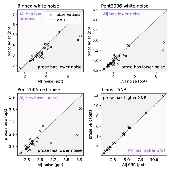
Figure 6: Noise and transit SNR comparison of prose against AstroImageJ (AIJ) on 26 TESS follow-up observations.

Figure 6 shows the results of our comparison: prose automatically yields light curves with lower white and red noise, resulting in transits recovered at slightly higher SNR on average. In this figure, the most discrepant points correspond to TOI-674, TOI-742, and TOI-2322 light curves (indexed 17, 24 and 26 in Table 4 and Figure 7). A careful reanalysis of these three datasets with AIJ was performed but could not explain these discrepancies.

AIJ does not require prior programming knowledge, making it a popular choice for professional astronomers as well as in the amateur astronomy community. Then, doing aperture photometry with AIJ requires the user to manually pick comparison stars (up to version 4) as well as a unique aperture size. In opposition, using standard Blocks in prose photometric pipeline allows to automatically detect stars, use a wide range of apertures and apply an automatic differential photometry algorithm, overall yielding light curves with lower noise. We note that, apart from alignment and centroiding aspects, AIJ and prose use similar algorithms (such as aperture photometry) which naturally leads to very comparable results. This validates the performances of prose default photometric pipeline against AIJ.

3.5 Processing time

The AIJ products used in our comparison were provided by several users with no information on the time required to do their complete reduction. In addition, prose provides measurements on a much larger number of stars and a wide range of apertures, making the comparison with AIJ uneven. That said, prose pipeline was developed with domestic computers in mind, an aspect which deserves to be quantified.

Given an observation, the reduction time of prose photometric pipeline depends on the number of images to process, their sizes, the number of stars to extract photometry on, the number of apertures considered, their radii, and of course the computer being used. Providing a figure for all these parameters is beyond the scope of this paper, instead we provide a figure which can be easily adapted to estimate the time required to reduce a given observation. Our sample contains $2096\times 2080$ pixels images on which we consider the 100 brightest stars using 40 apertures. We performed our reductions on a 3 Ghz Intel core i5 processor and 8Gb of RAM, taking an average of 10 $ms$ per image per star, which translates into 8 minutes for a typical 500 frames observation with photometry extracted on 100 stars and 40 apertures.

3.6 Reports

TESS candidates follow-ups are meant to be reported to the TFOP community. We wished to provide advanced reporting capabilities and developed a reporting framework adapted to prose products. Our reports consist in LaTeX templates that can be instantiated and automatically filled from Python scripts. While reports contain general sections, some TESS-specific pages were added, providing all the information related to TFOP activities. An example of such report is provided in Appendix B but its complete description is beyond the scope of this paper. For that, we refer the interested readers to the prose online documentation.

4 Conclusion

Initiatives like Astropy (Astropy Collaboration et al., 2013, 2018) and its affiliated packages (such as photutils (Bradley et al., 2020)) succeeded in offering an alternative to community tools like IRAF (Tody, 1986), whose support and use is progressively fading. However, building and testing a complete image processing pipeline using these tools requires software development skills and time, and often leads to poorly maintainable solutions.

We presented prose, a Python package to build modular image processing pipelines out of reusable Blocks. To demonstrate its potential, we used it to develop a basic photometric reduction pipeline that we compared to the one of AstroImageJ (Collins et al., 2017), a reference software at the center of the TESS candidates follow-up effort. Hence, we focused our comparison on 26 TESS follow-up observations and showed that prose, modular and instrument-agnostic, led to light curves with reduced white and red noise compared to the ones produced with AstroImageJ. Beyond its gain in precision, our pipeline requires close to no user interaction (apart from target selection) and leads to products benefiting from the advanced reporting capabilities of prose, all directly exploitable in Python.

Applications of prose extend beyond its base photometric pipeline. As an example, it was recently used to reduce slitless spectroscopy data from Hubble Space Telescope WFC3 observations (Garcia et al., 2021 in prep.). This development led to Blocks, independently maintainable, that will soon be available to the community, potentially useful in other applications. By adopting this modular approach, we hope to see the development of transparent pipelines which can live beyond individuals projects, serving the entire community, and leading to reproducible results.

We make prose open-source under the MIT license in a version controlled repository.

Data availability

The example data used in subsection 1.4 are privately held by the TRAPPIST team and can be requested by contacting the authors. On the other hand, some of the TESS follow-up observations used in this paper are available through the ExoFOP-TESS webpage. Raw images from the TRAPPIST telescope (listed in Table 4), as well as their photometric products (prose and/or AIJ) can be requested to the authors.

Appendix A Observations

A.1 AIJ comparison dataset

Table 4 summarizes our comparison dataset. Figure 7 shows the light curves obtained from these observations, using prose and AIJ.

index	telescope	date	target	filter	type
1	TRAPPIST-South	2018 10 01	TOI-145	z	other
2	TRAPPIST-South	2018 10 18	TOI-142	I+z	transit
3	TRAPPIST-South	2018 11 03	TOI-169	B	transit
4	TRAPPIST-South	2018 11 25	TOI-207	I+z	transit
5	TRAPPIST-South	2018 11 28	TOI-212	z	transit
6	TRAPPIST-South	2018 11 29	TOI-171	B	transit
7	TRAPPIST-South	2018 12 14	TOI-273	I+z	other
8	TRAPPIST-South	2018 12 15	TOI-270	z	transit
9	TRAPPIST-South	2018 12 19	TOI-150	B	transit
10	TRAPPIST-South	2018 12 27	TOI-270	z	transit
11	TRAPPIST-South	2019 01 12	TOI-350	I+z	transit
12	TRAPPIST-South	2019 02 16	TOI-442	z	transit
13	TRAPPIST-South	2019 03 24	TOI-500	B	transit
14	TRAPPIST-South	2019 03 27	TOI-504	RC	transit
15	TRAPPIST-South	2019 04 17	TOI-602	z	transit
16	TRAPPIST-South	2019 05 13	TOI-674	I+z	transit
17	TRAPPIST-South	2019 05 21	TOI-674	z	transit
18	TRAPPIST-South	2020 11 21	TOI-370.01	z	transit
19	TRAPPIST-South	2020 12 02	TOI-713.02	z	transit
20	TRAPPIST-South	2020 12 12	TOI-2202.01	I+z	transit
21	TRAPPIST-South	2020 12 13	TOI-2407.01	I+z	transit
22	TRAPPIST-South	2020 12 19	TOI-2416.01	z	transit
23	TRAPPIST-South	2020 12 24	TOI-2202.01	I+z	transit
24	TRAPPIST-South	2021 01 07	TOI-542.01	Exo	other
25	TRAPPIST-South	2021 01 17	TOI-736.02	I+z	transit
26	TRAPPIST-South	2021 01 24	TOI-2322.01	z	other

Table 4: Observations used for comparison with AIJ.

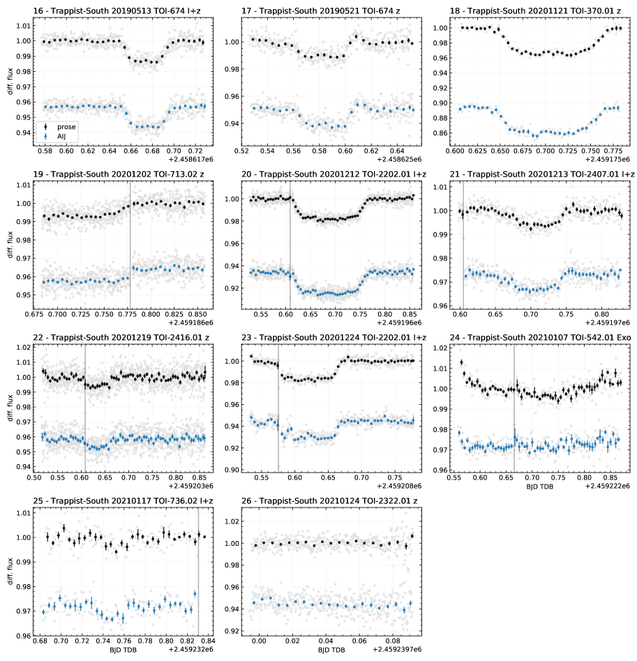
Figure 7: Comparison dataset light curves obtained from prose (black) and AIJ (blue). Differential fluxes are plotted in light gray and supplemented by binned colored points (binning of 0.05 days) with an error bar that corresponds to the standard deviation of points within each bin. When it is relevant, the vertical gray line indicates the time of meridian flip. Light curves shown in this figure are detrended from a meridian flip step signal and an order two polynomial of time, simultaneously fitted with a transit signal as described in subsection 3.3. We bring the reader’s attention to the fact that, unlike the signals shown in this figure, the four metrics presented in subsection 3.3 are evaluated on light curves cleaned from transit signals. Observations indexes (as defined in Table 4) are indicated in the title of each plot)

Appendix B TESS reports

Figure 8 and Figure 9 show elements of a TESS follow-up report produced with prose using LaTeX. While the first Summary page is automatically generated, other pages are pre-filled and can be freely complemented with figures and text.

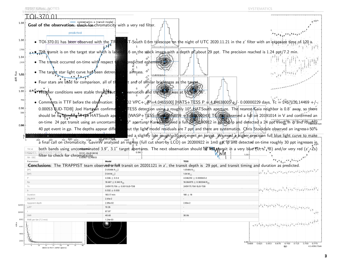
Figure 8: prose reports start with a Summary page, which intends to provide a quick look to an observation and its main products. The left side of this page features a stack image with the detected stars, among which are highlighted the target star (in blue) and comparison stars (yellow) used to build the differential light curves. At the bottom left, a cutout around the target as well as a radial PSF is plotted and the corresponding aperture overlaid. The rest of the page displays the raw and differential flux of the target star, as well as external parameters time-series (e.g. airmass) and comparison stars’ light curves.

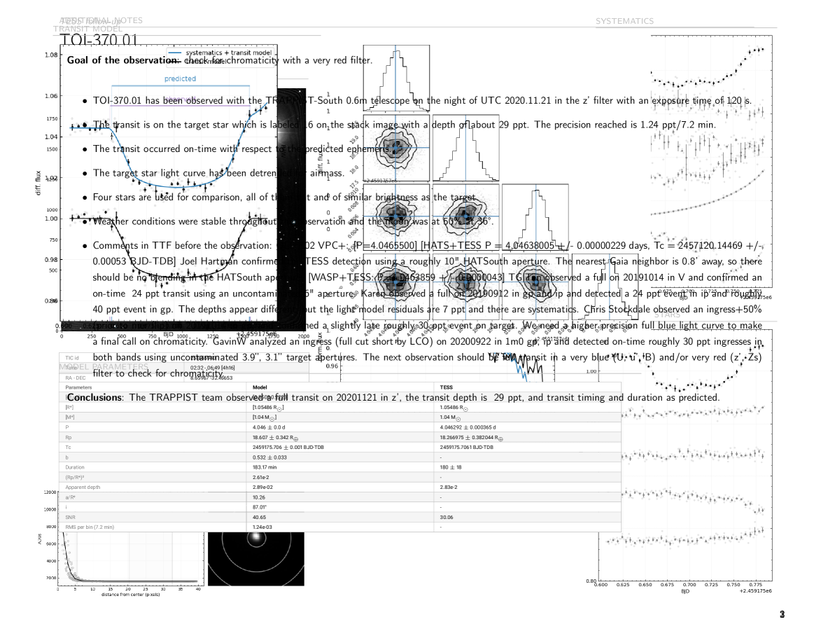
Figure 9: The Transit model report page shows a model of the transit light curve together with the inferred transit parameters (here a corner plot has been added manually). This model was inferred using the exoplanet Python package (Foreman-Mackey et al., 2021) and the corner plot done with corner (Foreman-Mackey, 2016).

References

- Astropy Collaboration et al. (2013) Astropy Collaboration, Robitaille, T. P., Tollerud, E. J., et al. 2013, A&A, 558, A33, doi: 10.1051/0004-6361/201322068
- Astropy Collaboration et al. (2018) Astropy Collaboration, Price-Whelan, A. M., Sipőcz, B. M., et al. 2018, AJ, 156, 123, doi: 10.3847/1538-3881/aabc4f
- Bertin & Arnouts (1996) Bertin, E., & Arnouts, S. 1996, A&AS, 117, 393, doi: 10.1051/aas:1996164
- Bradley et al. (2020) Bradley, L., Sipőcz, B., Robitaille, T., et al. 2020, astropy/photutils: 1.0.0, 1.0.0, Zenodo, doi: 10.5281/zenodo.4044744
- Broeg et al. (2005) Broeg, C., Fernández, M., & Neuhäuser, R. 2005, Astronomische Nachrichten, 326, 134, doi: 10.1002/asna.200410350
- Collins et al. (2017) Collins, K. A., Kielkopf, J. F., Stassun, K. G., & Hessman, F. V. 2017, AJ, 153, 77, doi: 10.3847/1538-3881/153/2/77
- Foreman-Mackey (2016) Foreman-Mackey, D. 2016, The Journal of Open Source Software, 1, 24, doi: 10.21105/joss.00024
- Foreman-Mackey et al. (2021) Foreman-Mackey, D., Luger, R., Agol, E., et al. 2021, arXiv e-prints, arXiv:2105.01994. https://arxiv.org/abs/2105.01994
- Foster et al. (2018) Foster, J. J., Smolka, J., Nilsson, D.-E., & Dacke, M. 2018, Proceedings of the Royal Society B: Biological Sciences, 285, 20172322, doi: 10.1098/rspb.2017.2322
- Gillon et al. (2011) Gillon, M., Jehin, E., Magain, P., et al. 2011, in European Physical Journal Web of Conferences, Vol. 11, European Physical Journal Web of Conferences, 06002, doi: 10.1051/epjconf/20101106002
- Head & Zerner (1985) Head, J. D., & Zerner, M. C. 1985, Chemical Physics Letters, 122, 264, doi: https://doi.org/10.1016/0009-2614(85)80574-1
- Herbel et al. (2018) Herbel, J., Kacprzak, T., Amara, A., Refregier, A., & Lucchi, A. 2018, J. Cosmology Astropart. Phys, 2018, 054, doi: 10.1088/1475-7516/2018/07/054
- Howell (2006) Howell, S. B. 2006, 1, Vol. 5, Handbook of CCD Astronomy
- Huber (1964) Huber, P. J. 1964, The Annals of Mathematical Statistics, 35, 73 , doi: 10.1214/aoms/1177703732
- Jehin et al. (2011) Jehin, E., Gillon, M., Queloz, D., et al. 2011, The Messenger, 145, 2
- Kingma & Ba (2017) Kingma, D. P., & Ba, J. 2017, Adam: A Method for Stochastic Optimization. https://arxiv.org/abs/1412.6980
- Lang et al. (2010) Lang, D., Hogg, D. W., Mierle, K., Blanton, M., & Roweis, S. 2010, The Astronomical Journal, 139, 1782–1800, doi: 10.1088/0004-6256/139/5/1782
- Moffat (1969) Moffat, A. F. J. 1969, A&A, 3, 455
- Pont et al. (2006) Pont, F., Zucker, S., & Queloz, D. 2006, MNRAS, 373, 231, doi: 10.1111/j.1365-2966.2006.11012.x
- Protopapas et al. (2005) Protopapas, P., Jimenez, R., & Alcock, C. 2005, MNRAS, 362, 460, doi: 10.1111/j.1365-2966.2005.09305.x
- Stetson (1987) Stetson, P. B. 1987, PASP, 99, 191, doi: 10.1086/131977
- Tody (1986) Tody, D. 1986, in Society of Photo-Optical Instrumentation Engineers (SPIE) Conference Series, Vol. 627, Instrumentation in astronomy VI, ed. D. L. Crawford, 733, doi: 10.1117/12.968154
- Wells & Greisen (1979) Wells, D. C., & Greisen, E. W. 1979, in Image Processing in Astronomy, ed. G. Sedmak, M. Capaccioli, & R. J. Allen, 445