On Similarity

Abstract

The objective quantification of similarity between two mathematical structures constitutes a recurrent issue in science and technology. In the present work, we developed a principled approach that took the Kronecker’s delta function of two scalar values as the prototypical reference for similarity quantification and then derived for more yielding indices, three of which bound between 0 and 1. Generalizations of these indices to take into account the sign of the scalar values were then presented and developed to multisets, vectors, and functions in real spaces. Several important results have been obtained, including the interpretation of the Jaccard index as a yielding implementation of the Kronecker’s delta function. When generalized to real functions, the four described similarity indices become respective functionals, which can then be employed to obtain associated operations of convolution and correlation.

‘Springtime, always plentiful of most diverse similarities.’

LdaFC

1 Introduction

It is often mentioned that one of the most important aspects of science is the quantification of the physical world structures and phenomena, through respective measurements, so as to allow the development of objective theories. While this is certainly true, there is a complementary aspect to taking measurements, and this concerns comparing and ordering the obtained quantifications so as to be able to take decisions on the most plausible models and explanations.

For instance, given a model, its ability to account for the respectively modeled systems consists of comparing not only scalar values, but vectors, matrices, functions, as well as potentially any other mathematica structure. Indeed, the own validation of models and theories rely critically on several logical and quantitative indications of similarity.

In addition to the critically important role of comparisons in science, living beings also continuously rely on comparing entities, be then a received stimuli or more complex mental representations. For instance, we humans are always comparing today’s weather with those of other times.

Comparing things in an objective quantitative manner involves the adoption of one or more measurements of similarity or distance between pairs of values, of which the Euclidean distance seems to have a particular importance.

On subsequent scales, measurements are also required for comparing sets of objects, and here the cosine similarity and Jaccard indices (e.g. [1, 2]) are often employed. At an even higher level, we need approaches capable of quantifying the similarity between functions, in which case the inner product, and the respectively derived operations of convolution and correlation, are often adopted (e.g. [3, 4, 5, 6]).

Given that similarity and distance are intrinsically interrelated, including the fact that one can often be derived from the other, the present work will focus only on similarity measurements, with the obtained results being immediately extensible to distances.

Interestingly, the Euclidian distance, cosine similarity and inner product all share a same aspect, which consists in being based on products between pairs of values. As such, these approaches can be said to have a second order nature ($x.x=x^{2}$). However, there is a virtually infinite number of other possible distance and similarity measurements, including those based on minimum, maximum and absolute values.

In the present work, we aim at developing a principled approach in which we start by contemplating the similarity between two scalar real values $x$ and $y$, from which it is concluded that the Kronecker’s delta function provides a prototypical reference. However, given that this approach is too strict, it becomes necessary to relax the Kronecker’s delta function criterion so as to obtain more yielding respective similarity indices. Four main possibilities are identified, three of which being suitably bound in the interval $[0,1]$, being denominated $s_{1}$, $s_{2}$, $s_{3}$, and $s_{4}$.

Then, by using concepts derived from [1, 2], we describe how these four indices can be generalized in order to provide additional information about the relative alignment between the two compared scalar values, yielding 4 respective versions of the adopted indices.

These indices are then further generalized, again by considering the results in [1, 2], to multisets (e.g. [7, 8, 9, 10, 11, 12]), vectors, and real functions. Though respective extensions to other mathematical structures including matrices, graphs, and scalar and vector fields are analogous, we do not develop these possibilities in the present work.

Two other similarity indices, namely the interiority (or homogeneity) and coincidence indices [1, 2, 13], are also presented in their generalized versions for functions. In particular, the coincidence index has been found to present enhanced performance in important tasks such as pattern recognition [13] as well as when extended to act as quantifiers of joint variation between random variables [1, 14].

When generalized to real function spaces, the four indices become functionals and, as such, can be combined in several manners and also used to implement respective convolution and correlation binary operations between functions.

Among the several interesting results obtained, we have that the indices proposed in [1], especially the coincidence and addition-based mset Jaccard indices, actually corresponds to the generalizations of the scalar indices $s_{1}$ and $s_{2}$.

We start by deriving the four similarity index from the Kronecker’s delta function, and proceed by presenting their extension to negative values and further generalization to multisets, vectors, and functions. Generalizations of the interiority and continuity indices to multisets, vectors and functions possibly taking negative values are then presented, which is followed by the presentation of the employment of all considered indices to define respective convolutions and correlations.

2 Pairwise Similarities in $\mathbb{R}$

Before proceeding in depth with any current study of distances, it is important to state as objectively as possible what is being meant by similarity. Unlike the concept of distance, which is ubiquitously associated to the concept of Euclidean distance, there seems to be less consensus regarding what similarity means.

In this work, we will understand similarity between two values $x$ and $y$ in the sense of identity between them. Figure 1 illustrates the most strict approach to quantifying the similarity between any two real values $x$ and $y$, which assigns 1 whenever $x=y$, and $0$ otherwise.

Figure 1: The most strict quantification of the similarity between two real values $x$ and $y$, implemented via a similarity binary operator $\delta_{x,y}$ that corresponds to the Kronecker delta. A non-zero result is obtained only in case $x=y$.

For simplicity’s sake, the case $(x=0,y=0)$ is not considered in this work. Therefore, additional checking and handling is required in situations in which these values are viable.

Mathematically, this strict similarity quantification corresponds to a continuous Dirac delta comb function $\delta_{x,y}$.

The problem with this approach evidently is that it is way too strict, so that it becomes necessary to provide means for implementing some tolerance in the quantification.

The distance between any vector $\left[x,y\right]$ and the line $y=x$ can be readily expressed as:

$$d\left(\vec{p}=\left[x,y\right],\hat{u}=\left[\frac{1}{\sqrt{2}},\frac{1}{\sqrt{2}}\right]\right)=\frac{|x-y|}{\sqrt{2}}$$ (1)

Observe that this function is not upper bound, i.e. all we can say is that $0\leq d\left(\vec{p},\hat{u}\right)$.

A possible manner to bound this distance is by making:

$$\tilde{d}\left(\vec{p},\hat{u}\right)=\frac{|x-y|}{\max\left\{|x|,|y|\right\}}$$ (2)

which now ensures that $0\leq\tilde{d}\left(\vec{p},\hat{u}\right)\leq 1$.

Having a distance measurement normalized in the interval $[0,1]$ is of critical importance because it allows us to derive a respective similarity distance simply as:

$$s\left(\vec{p},\hat{u}\right)=1-\frac{|x-y|}{\max\left\{|x|,|y|\right\}}$$ (3)

It can be verified that:

$$1-\frac{|x-y|}{\max\left\{|x|,|y|\right\}}=\frac{2\min\left\{|x|,|y|\right\}}{|x|+|y|}$$ (4)

which is a slightly more convenient manner to express this similarity, which will constitute one of the similarity index addressed in the present work:

$$s_{1}(x,y)=\frac{2\min\left\{|x|,|y|\right\}}{|x|+|y|}$$ (5)

with $0\leq s_{1}(x,y)\leq 1$.

This similarity measurement is illustrated in Figure 2.

Figure 2: Two pairs of values $(x_{a},y_{a})$ and $(x_{b},y_{b})$ are to be compared in terms of similarity. In the former case, we have that $\max\left\{x_{a},y_{a}\right\}=x_{a}$ and $\min\left\{x_{a},y_{a}\right\}=y_{a}$, with $x_{a}\neq y_{a}$, yielding a respective similarity smaller than one. In the other case, we will also have a similarity smaller than one for similar reasons. Actually, because of the intrinsic symmetry in this case, the two obtained values of $s_{1}$ will be identical.

The average between $|x|$ and $|y|$ can now be replaced by $\max\left\{|x|,||y|\right\}$, yielding another normalized similarity index:

$$s_{2}(x,y)=\frac{\min\left\{|x|,|y|\right\}}{\max\left\{|x|,|y|\right\}}$$ (6)

with $0\leq s_{2}(x,y)\leq 1$.

Yet another possible modification of the similarity index in Equation 5 can be obtained by considering the product of functions:

$$s_{3}=\frac{|x||y|}{\left(\max\left\{|x|,|y|\right\}\right)^{2}}\\$$ (7)

with $0\leq s_{3}(x,y)\leq 1$.

It is also interesting to consider the following unbound version of the index $s_{3}$:

$$s_{4}=|x||y|$$ (8)

with $0\leq s_{4}\leq\infty$.

Though other similarity indices can be derived in analogous manner, the present work will focus on the three indices $s_{1}$, $s_{2}$ and $s_{3}$ above.

Now, it is interesting to realize that the above indices loose information about the relative signs of the involved quantities. While this feature is suitable, and even desired in some circumstances, it is important to have generalizations of the three similarity indices derived above that can take into account the signs of the involved quantities.

Consider the situations depicted in Figure 3. Here, we have the four situations which needed to be taken into account while generalizing the three adopted similarity indices to cope with negative values.

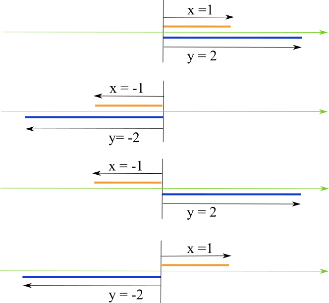
Figure 3: The four main situations met when comparing two positions $x$ and $y$ along the real line $\mathbb{R}$. It is often interesting to take into account whether the positions point toward the same or opposite directions.

The similarity sign should express whether the two positions point toward the same direction, which case a positive similarity could be expected, or it they oppose one another, yielding a respective negative similarity sign.

The key to obtaining signed similarity consists in employing the following functions:

$$s_{x}=\emph{sign}(x)$$ (9)

$$s_{y}=\emph{sign}(y)$$ (10)

$$s_{xy}=\emph{sign}(x)\;\emph{sign}(y)$$ (11)

We shall refer to the function $s_{xy}$ as the conjoint sign function.

We can now generalize the three adopted similarity index to reflect the sign of the values $x$ and $y$ as:

$$s_{1}=s_{xy}\frac{\min\left\{s_{x}x,s_{y}y\right\}}{\max\left\{s_{x}x,s_{y}y\right\}}$$ (12)

$$s_{2}=s_{xy}\frac{2\min\left\{s_{x}x,s_{y}y\right\}}{s_{x}x+s_{y}y}$$ (13)

$$s_{3}=\frac{xy}{\left(\max\left\{s_{x}x,s_{y}y\right\}\right)^{2}}$$ (14)

$$s_{4}=s_{xy}(s_{x}xs_{y}y)=s_{xy}^{2}xy=xy$$ (15)

with $-1\leq s_{1},s_{2},s_{3}\leq 1$ and $-\infty\leq s_{4}\leq\infty$.

For simplicity’s sake, both the modulus and signed versions of the three similarities will be henceforth referred to simply as $s_{1}$, $s_{2}$, and $s_{3}$, as the context shall be enough to indicate how they are being applied.

In the context of polynomials, the product of two values $x$ and $y$ represents a second degree operation. This operation has an intrinsic characteristic in which the product of two numbers larger than one tend to increase steeply with the magnitude of the values. However, when two values with magnitude smaller than 1 are multiplied, the resulting value is typically substantially reduced. This characteristic is a direct consequence of the non-bilinearity of the product operation.

Interestingly, the results from $s_{1}$ to $s_{4}$ can be understood as providing successively blurred versions of the Kronecker’s delta reference similarity functions. Therefore, more strict quantifications of similarity between two values $x$ and $y$ will be provided by $s_{1}$ and $s_{2}$, while $s_{3}$ and $s_{4}$ represent particularly yielding alternatives.

Figure 4 illustrates the four proposed similarity indices in the region bound by $x\in[-1,1]$ and $y\in[-1,1]$. Both $s_{1}$ (a) and $s_{2}$ (b) yields marked peaks with value 1 along the main diagonal, indicating the close relationship between these two similarity indices and the Kronecker’s delta function. This diagonal peak is much less marked in the case of $s_{3}$ (c), and virtually undistinguishable in $s_{4}$.

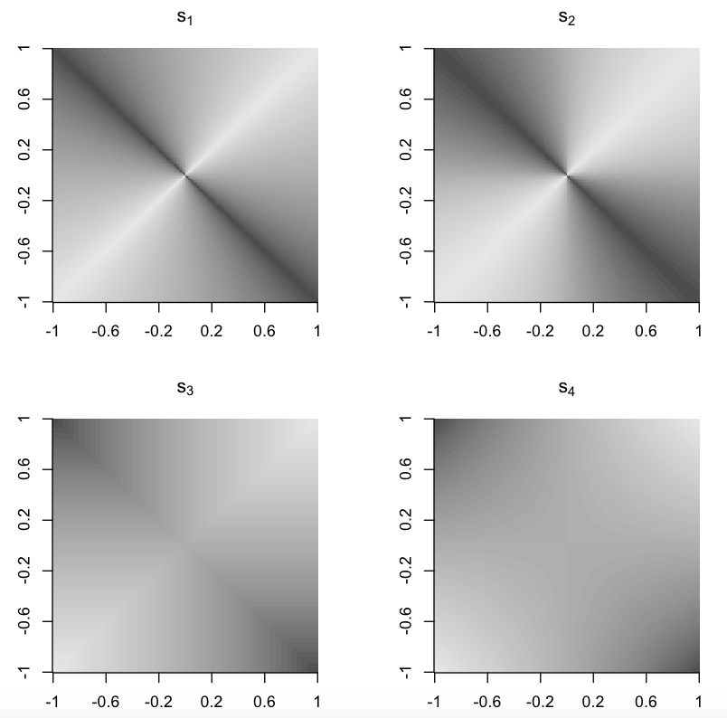
Figure 4: The values of the four proposed similarity indices in the region bound by $x\in[-1,1]$ and $y\in[-1,1]$. The gray scale varies from 0 to 1. Observe the peak main diagonal in cases (a) and (b), which have a direct relationship with the Kronecker’s delta and can be understood as a respectively smoothed version.

Perhaps the most important interpretation of Figure 4 consists in the fact that the similarity measurements $s_{4}$ — upon which the inner product and standard convolution, correlation, as well as the covariance statistical concept are based — does not penalize the region adjacent to the secondary diagonal $y=-x$. It is precisely this characteristic of this index that accounts for the tendency of the Pearson correlation coefficient (e.g. [15]), which is derived from this index, to overestimate the joint variation in cases where the two variables are not strongly related [1].

Figure 5 illustrates scatterplots obtained with respect to each pairwise association between the four indices $s_{1}$, $s_{2}$, $s_{3}$ and $s_{4}$. Interestingly, the first two indices are closely related and bijectively associated. This is not the case with the fourth and fifth indices which, though similar (consider the respective scatterplot in the figure) are not bijective one another and much less with the other two indices.

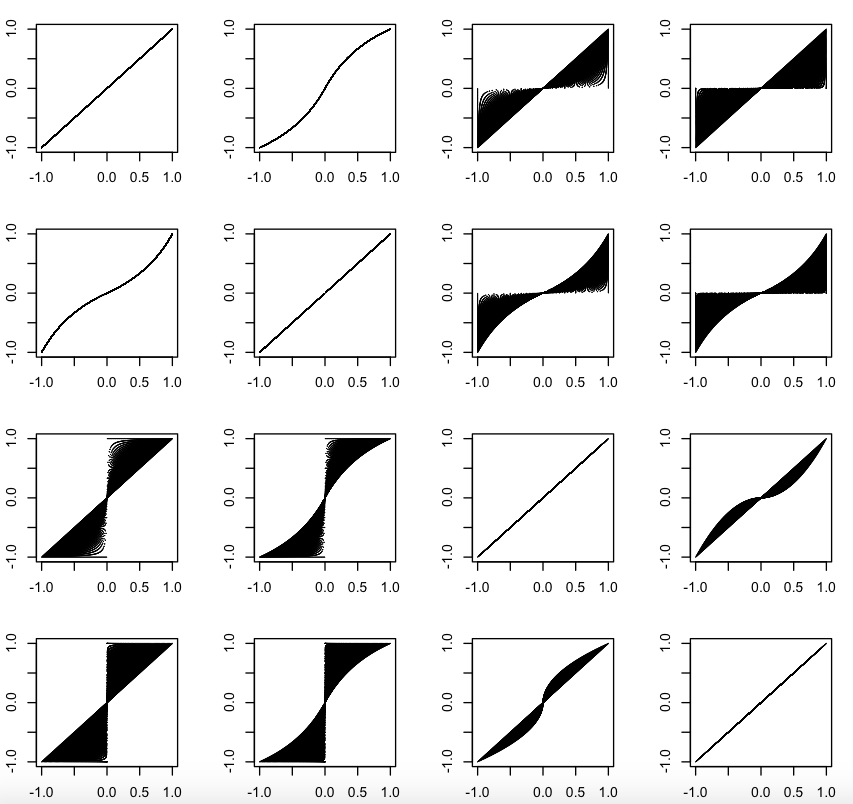
Figure 5: Scatterplots illustrating the joint relationship between each pair of the four similarity indices $s_{1}$, $s_{2}$, $s_{3}$ and $s_{4}$.

3 Multiset Similarities

Now that we have developed a principled approach to quantifying the similarity between two real values $x$ and $y$, it becomes possible to extend these indices to other mathematical structures, including multisets, vectors, functions, etc. In this section we address the important subject of quantifying the similarity between two multisets, which are henceforth referred to as msets.

A multiset $A$ can be represented as:

$$A=\{\kern-2.15277pt|\left[a_{1},m_{A}(a_{1})\right];\left[a_{2},m_{A}(a_{2})\right];\ldots;\left[a_{N},m_{A}(a_{N})\right]|\kern-2.15277pt\}$$

where we have $N$ elements $a_{i}$, each with respective multiplicity $m_{A}(a_{i})$. The support of this multiset is $S_{A}=\left\{a_{1},a_{2},\ldots,a_{N}\right\}$.

The union of two msets $A$ and $B$ sharing the same support is defined as:

$$A\cup B=\{\kern-2.15277pt|\left[a_{1},\max\left\{m_{A}(a_{1}),m_{B}(a_{1})\right\}\right];$$

$$\left[a_{2},\max\left\{m_{A}(a_{2}),m_{B}(a_{2})\right\}\right];\ldots;$$

$$\left[a_{N},\max\left\{m_{A}(a_{N}),m_{B}(a_{N})\right\}\right]|\kern-2.15277pt\}$$ (16)

In case $A$ and $B$ do not share the same support, a respective support can be obtained for the mset union consisting of the set union of the respective mset supports.

The intersection between two msets $A$ and $B$ sharing the same support is given as:

$$A\cap B=\{\kern-2.15277pt|\left[a_{1},\min\left\{m_{A}(a_{1}),m_{B}(a_{1})\right\}\right];$$

$$\left[a_{2},\min\left\{m_{A}(a_{2}),m_{B}(a_{2})\right\}\right];\ldots;$$

$$\left[a_{N},\min\left\{m_{A}(a_{N}),m_{B}(a_{N})\right\}\right]|\kern-2.15277pt\}$$ (17)

Msets can be generalized to real multiplicities, including possibly negative values [1, 2].

Quantification indices of the elementwise similarity between two multisets $A$ and $B$ can be immediately obtained by applying the four scalar similarity indices proposed in the previous section.

For simplicity’s sake, we shall abbreviate $m_{A}(a_{i})$ as $x_{i}$, and $m_{B}(a_{i})$ as $y_{i}$, which then yields:

$$s_{1}(x_{i},y_{i})=s_{x_{i}y_{i}}\frac{\min\left\{s_{x_{i}}x_{i},s_{y_{i}}y_{i}\right\}}{\max\left\{s_{x_{i}}x_{i},s_{y_{i}}y_{i}\right\}}$$ (18)

$$s_{2}(x_{i},y_{i})=s_{x_{i}y_{i}}\frac{2\min\left\{s_{x_{i}}x_{i},s_{y_{i}}y_{i}\right\}}{s_{x_{i}}x_{i}+s_{y_{i}}y_{i}}$$ (19)

$$s_{3}(x_{i},y_{i})=\frac{x_{i}y_{i}}{\left(\max\left\{x_{i},y_{i}\right\}\right)^{2}}$$ (20)

$$s_{4}(x_{i},y_{i})=x_{i}y_{i}$$ (21)

It is of particular interest to generalize the four indices to quantify the similarity between two multisets $A$ and $B$, which can be done as:

$$s_{1}(A,B)=\frac{\sum_{i}s_{x_{i}y_{i}}\min\left\{s_{x_{i}}x_{i},s_{y_{i}}y_{i}\right\}}{\sum_{i}\max\left\{s_{x_{i}}x_{i},s_{y_{i}}y_{i}\right\}}$$ (22)

$$s_{2}(A,B)=\frac{2\sum_{i}s_{x_{i}y_{i}}\min\left\{s_{x_{i}}x_{i},s_{y_{i}}y_{i}\right\}}{\sum_{i}\left[s_{x_{i}}x_{i}+s_{y_{i}}y_{i}\right]}$$ (23)

$$s_{3}(A,B)=\frac{\sum_{i}x_{i}y_{i}}{\sum_{i}\left(\max\left\{s_{x_{i}}x_{i},s_{y_{i}}y_{i}\right\}\right)^{2}}$$ (24)

$$s_{4}(A,B)=\frac{\sum_{i}x_{i}y_{i}}{|A||B|}$$ (25)

The resulting index $s_{1}$ for msets is corresponds to the generalization of the Jaccard similarity index to negative values [1, 2] $J_{N}$, while the index $s_{2}$ results identical to the also recently proposed addition-based mset Jaccard index (e.g. [1, 2]), i.e.:

$$s_{1}(A,B)=J_{N}(A,B)$$ (26)

Therefore, the developments above allowed a principled derivation of those recently introduced generalizations of the Jaccard similarity index (e.g. [16, 17]).

It also follows from the above developments that the generalized Jaccard index can be understood as an implementation of smoothed generalizations of the Kronecker’s delta function based similarity to scalars, msets, vectors and scalar fields.

4 Vector Similarities

Since vectors can be understood as particular cases of msets with support $S=\{\kern-2.15277pt|1,2,\ldots,N|\kern-2.15277pt\}$, the respective generalization of the proposed similarity to this type of mathematical structures is immediate.

Let two vectors $\vec{x}=\left[x_{1},x_{2},\ldots,x_{N}\right]$ and $\vec{y}=\left[y_{1},y_{2},\ldots,y_{N}\right]$. We then have:

$$s_{1}(x_{i},y_{i})=s_{x_{i}y_{i}}\frac{\min\left\{s_{x_{i}}x_{i},s_{y_{i}}y_{i}\right\}}{\max\left\{s_{x_{i}}x_{i},s_{y_{i}}y_{i}\right\}}$$ (27)

$$s_{2}(x_{i},y_{i})=s_{x_{i}y_{i}}\frac{2\min\left\{s_{x_{i}}x_{i},s_{y_{i}}y_{i}\right\}}{s_{x_{i}}x_{i}+s_{y_{i}}y_{i}}$$ (28)

$$s_{3}(x_{i},y_{i})=\frac{x_{i}y_{i}}{\left(\max\left\{x_{i},y_{i}\right\}\right)^{2}}$$ (29)

$$s_{4}(x_{i},y_{i})=x_{i}y_{i}$$ (30)

from which:

$$s_{1}(\vec{x},\vec{y})=\frac{\sum_{i}s_{x_{i}y_{i}}\min\left\{s_{x_{i}}x_{i},s_{y_{i}}y_{i}\right\}}{\sum_{i}\max\left\{s_{x_{i}}x_{i},s_{y_{i}}y_{i}\right\}}$$ (31)

$$s_{2}(\vec{x},\vec{y})=\frac{2\sum_{i}s_{x_{i}y_{i}}\min\left\{s_{x_{i}}x_{i},s_{y_{i}}y_{i}\right\}}{\sum_{i}\left[s_{x_{i}}x_{i}+s_{y_{i}}y_{i}\right]}$$ (32)

$$s_{3}(\vec{x},\vec{y})=\frac{\sum_{i}x_{i}y_{i}}{\sum_{i}\left(\max\left\{s_{x_{i}}x_{i},s_{y_{i}}y_{i}\right\}\right)^{2}}$$ (33)

$$s_{4}(\vec{x},\vec{y})=\frac{\sum_{i}x_{i}y_{i}}{|\vec{x}||\vec{y}|}$$ (34)

Observe that the index $s_{4}$ becomes identical to the inner product between the two vectors.

5 Function Similarities

The generalization of the similarity indices to real functions follows directly from the mset continuous representation [1, 2].

Given two real-valued functions $f(x)$ and $g(x)$ with shared support $S$, we immediately have:

$$s_{1}(f(x),g(x))=s_{x_{f(x)g(x)}}\frac{\min\left\{s_{f(x)}f(x),s_{g(x)}g(x)\right\}}{\max\left\{s_{f(x)}f(x),s_{g(x)}g(x)\right\}}$$ (35)

$$s_{2}(f(x),g(x))=s_{f(x)g(x)}\frac{2\min\left\{s_{f(x)}f(x),s_{g(x)}g(x)\right\}}{s_{f(x)}f(x)+s_{g(x)}g(x)}$$ (36)

$$s_{3}(f(x),g(x))=\frac{f(x)g(x)}{\left(\max\left\{f(x),g(x)\right\}\right)^{2}}$$ (37)

$$s_{4}(f(x),g(x))=f(x)g(x)$$ (38)

So that the respective functionals can be written as:

$$s_{1}(f,g)=\frac{\int_{S}s_{fg}\min\left\{s_{f}f,s_{g}g\right\}dx}{\int_{S}\max\left\{s_{f}f,s_{g}g\right\}dx}$$ (39)

$$s_{2}(f,g)=\frac{2\int_{S}s_{fg}\min\left\{s_{f}f,s_{g}g\right\}dx}{\int_{S}\left[s_{f}f+s_{g}g\right]dx}$$ (40)

$$s_{3}(f,g)=\frac{\int_{S}fg\ dx}{\int_{S}\left(\max\left\{s_{f}f,s_{g}g\right\}\right)^{2}dx}$$ (41)

$$s_{4}(f,g)=\frac{\int_{S}fg\ dx}{|f||g|}$$ (42)

where $f(x)$ has been abbreviated as $f$, $g(x)$ has been abbreviated as $g$, $|f|=\int_{S}|f(x)|dx$ and $|g|=\int_{S}|g(x)|dx$.

Another interesting implication of the similarity indices generalized to real functions is that they can be understood as corresponding to binary operations, in particular the product, between two functionals.

For instance, in the case of Equation 39, we can write:

$$s_{1}(f,g)=\frac{\ll f,g\gg}{f\diamond g}$$ (43)

where:

$$\ll f,g\gg\ =\int_{S}s_{fg}\min\left\{s_{f}f,s_{g}g\right\}dx$$ (44)

which has been called the common product between $f$ and $g$ [1, 2, 13, 18].

and:

$$f\diamond g=\int_{S}\max\left\{s_{f}f,s_{g}g\right\}dx$$ (45)

which can be understood as a functional acting on the union of the absolute valued versions of $f$ and $g$.

The other three similarities indices imply similar decompositions.

The functionals $\ll f,g,\gg$, $f\diamond g$ act on the following elementwise respective products:

$$\ll f,g\gg_{p}\ =s_{fg}\min\left\{s_{f}f,s_{g}g\right\}$$ (46)

$$(f\diamond g)_{p}=\max\left\{s_{f}f,s_{g}g\right\}$$ (47)

and it is also possible to define the elementwise operations related to the common product as:

$$s_{1,p}(f,g)=\frac{s_{fg}\min\left\{s_{f}f,s_{g}g\right\}}{\max\left\{s_{f}f,s_{g}g\right\}}\$$ (48)

However, observe that the functional $s_{1}(f,g)$ involves taking separated integrals of the numerator and denominator.

Figure 6 shows the elementwise operations $\ll f,g\gg_{p}$, $(f\diamond g)_{p}$, and $s_{1,p}(f,g)$ in the case of the sine and cosine function within one complete period. Observe these two functions shown as dashed lines in Figurefig:sincos(c). We can observe that $\ll f,g\gg_{p}$ reveals to the common area between the sine and cosine, while $(fdiamondg)_{p}$ is the maximum between the respective absolute values of these two functions. The result $s_{1}(f,g)$, provides an effective indication of the signed similarity between the two considered functions.

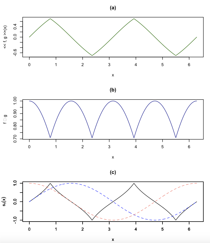
Figure 6: The elementwise operations $\ll f,g,\gg_{p}$, $f\diamond g_{p}$ and $s_{1,p}(f,g)$ obtained for a complete period of the sine and cosine functions.

6 The Interiority and Coincidence Indices

As shown in [1], the traditional Jaccard similarity index between two sets $A$ and $B$ is not capable of taking into account how much one of the sets is interior to the other. In order to compensate for this issue, a new similarity index, called coincidence index was proposed [1] as corresponding to the product between the traditional Jaccard index and the interiority (or homogeneity) index.

The interiority index can be expressed as:

$$I(A,B)=\frac{A\cap B}{\min\left\{|A|,|B|\right\}}$$ (49)

where $|A|$ and $|B|$ are the cardinalities of sets $A$ and $B$.

So that the coincidence index results as:

$$C(A,B)=I(A,B)J(A,B)$$ (50)

Where $J(A,B)$ is the conventional Jaccard index.

Both the interiority and coincidence indices can also be understood as corresponding to quantifications of similarities. As such, it becomes interesting to consider their generalizations to msets, vectors, and functions [1, 2, 18].

First, we consider the respective version of the interiority index allowing real multiplicities [1, 2, 13, 18]:

In the case of msets, we have:

$$I(A,B)=\frac{\sum_{i\in S_{+}}\min\left\{s_{x_{i}}x_{i},s_{y_{i}}y_{i}\right\}}{\min\left\{\sum_{i\in S_{+}}s_{x_{i}}x_{i},\;\sum_{i\in S_{+}}s_{y_{i}}y_{i}\right\}}$$ (51)

where $S_{+}$ is the support restricted to the situations in which $s_{x_{i}}s_{y_{i}}>0$. This restriction reflects the fact the understanding that it is impossible to have interiority between two msets with all respective elements having opposite sign multiplicities. Observe that, as a consequence, $0\leq I(A,B)\leq 1$.

In case the whole support is to be taken into account, which can be required in some circumstances such as when performing template matching [13], we can make:

$$I(A,B)=\frac{\sum_{i\in S}\min\left\{s_{x_{i}}x_{i},s_{y_{i}}y_{i}\right\}}{\min\left\{\sum_{i\in S}s_{x_{i}}x_{i},\;\sum_{i\in S}s_{y_{i}}y_{i}\right\}}$$ (53)

In the case of vectors, we immediately have:

$$I(\vec{x},\vec{y})=\frac{\sum_{i\in S_{+}}\min\left\{s_{x_{i}}x_{i},s_{y_{i}}y_{i}\right\}}{\min\left\{\sum_{i\in S_{+}}s_{x_{i}}x_{i},\;\sum_{i\in S_{+}}s_{y_{i}}y_{i}\right\}}$$ (55)

So that:

$$C(\vec{x},\vec{y})=I(\vec{x},\vec{y})J(\vec{x},B\vec{y})=I(\vec{x},\vec{y})\;s_{1}(\vec{x},B\vec{y})$$ (57)

And, for functions:

$$I(f,g)=\frac{\int_{S_{+}}\min\left\{s_{f}f,s_{g}g\right\}dx}{\min\left\{\int_{S_{+}}s_{f}fdx,\;\int_{S_{+}}s_{g}gdx\right\}}$$ (58)

Implying:

$$C(f,g)=I(f,g)J(f,g)=I(f,g)\;s_{1}(f,g)$$ (60)

7 Similarity Convolutions and Correlations

Each of the similarity indices generalized to the real space of functions corresponds to a valid functional. Now, it is possible to obtain respective convolutions and correlations. For instance, in the case of $s_{1}$, we have the following respectively associated convolution:

$$(f\Box g)_{s1}[y]=\frac{\int_{S}s_{fg}\min\left\{s_{f}f,s_{g}g(y-x)\right\}dx}{\int_{S}\max\left\{s_{f}f,s_{g}g(y-x)\right\}dx}\\$$ (61)

and correlation:

$$(f\blacksquare g)_{s1}[y]=\frac{\int_{S}s_{fg}\min\left\{s_{f}f,s_{g}g(x-y)\right\}dx}{\int_{S}\max\left\{s_{f}f,s_{g}g(x-y)\right\}dx}\\$$ (62)

In the case of $s_{4}$, we have:

$$(f\Box g)_{s4}[y]=\frac{\int_{S}s_{g}g(y-x)dx}{|f||g|}\\$$ (63)

which corresponds to a normalized version of the standard convolution.

Since the common product is associated to the Walsh functions [18], it is possible to perform convolutions involving these functions (e.g. [19, 20, 21, 22]) by using fast computing schemes (e.g. [23]) analogous to the fast Fourier transform (e.g. [3]).

Another interesting point is that, while the products in the Fourier transform are bilinear, the analogous counterpart in the common product is the non-linear operation of maximum. This confers some important properties to respective related operations, such as correlation, such as substantially enhanced performance in tasks such as template matching and filtering [13].

8 Concluding Remarks

The concept of similarity appears recurrently in science and technology, underlying a large number of concepts, operations, and properties. From the perspective of Hilbert spaces, the similarity is critically important as it is related to the concept of inner product on which those spaces are based. However, the quantification of similarities between mathematical entities also constitute an ubiquitous task in virtually every applied area, including but by no means limited to patter recognition, signal processing, and machine intelligence, to name but a few cases.

In the present work, we developed a principled approach in which the Kronecker’s delta function was taken as the prototypical reference for quantifying the similarity between two scalar values, and then developed more yielding versions involving the operations of minimum, maximum, sum and product, in addition to the sign function. Four main indices were obtained, three of which are normalized in the interval $[0,1]$, which were then extended to respective signed versions capable of providing more information about the kind of similarity, yielding respective versions of these indices bound by the interval $[-1,1]$.

Then, relying on recent results regarding the extension of multisets to functions and other mathematical structures [1, 2, 18], we were able to extend the four signed similarity indices to multisets, vectors, and then functions. The extension to other mathematical structures including scalar and vector fields can also be obtained in analogous manner.

Several important results have been obtained. First, we have that the extensively applied Jaccard index relates directly to the similarity index $s_{1}$, while the index $s_{4}$ let to the standard inner product functional and convolution. Of particular interest is that the similarity functionals recently introduced in [1, 2, 13, 14] resulted naturally from the here reported developments. For instance, it has been possible to verify that the mset Jaccard index, when adapted to negative values, corresponds to the functional respective to the described index $s_{1}$. In addition, the addition-based mset Jaccard index was shown to follow from the index $s_{2}$. The index $s_{4}$, which is unbound, led to the standard inner product and respectively associated convolution and correlation.

Acknowledgments.

Luciano da F. Costa thanks CNPq (grant no. 307085/2018-0) and FAPESP (grant 15/22308-2).

References

- [1] L. da F. Costa. Further generalizations of the Jaccard index. https://www.researchgate.net/publication/355381945_Further_Generalizations_of_the_Jaccard_Index, 2021. [Online; accessed 21-Aug-2021].
- [2] L. da F. Costa. Multisets. https://www.researchgate.net/publication/355437006_Multisets, 2021. [Online; accessed 21-Aug-2021].
- [3] E. O. Brigham. Fast Fourier Transform and its Applications. Pearson, 1988.
- [4] R. O. Duda, P. E. Hart, and D. G. Stork. Pattern Classification. Wiley Interscience, 2000.
- [5] K. Koutrombas and S. Theodoridis. Pattern Recognition. Academic Press, 2008.
- [6] L. da F. Costa and R. M. C. Cesar Jr. Shape Classification and Analysis: Theory and Practice. CRC Press, Boca Raton, 2nd edition, 2009.
- [7] J. Hein. Discrete Mathematics. Jones & Bartlett Pub., 2003.
- [8] D. E. Knuth. The Art of Computing. Addison Wesley, 1998.
- [9] W. D. Blizard. Multiset theory. Notre Dame Journal of Formal Logic, 30:36—66, 1989.
- [10] W. D. Blizard. The development of multiset theory. Modern Logic, 4:319–352, 1991.
- [11] P. M. Mahalakshmi and P. Thangavelu. Properties of multisets. International Journal of Innovative Technology and Exploring Engineering, 8:1–4, 2019.
- [12] D. Singh, M. Ibrahim, T. Yohana, and J. N. Singh. Complementation in multiset theory. International Mathematical Forum, 38:1877–1884, 2011.
- [13] L. da F. Costa. Comparing cross correlation-based similarities. https://www.researchgate.net/publication/355546016_Comparing_Cross_Correlation-Based_Similarities, 2021. [Online; accessed 21-Oct-2021].
- [14] L. da F. Costa. Coincidence component analysis. https://www.researchgate.net/publication/355752394_Coincidence_Component_Analysis_-_CCA, 2021. [Online; accessed 21-Oct-2021].
- [15] R. A. Johnson and D.W. Wichern. Applied multivariate analysis. Prentice Hall, 2002.
- [16] P. Jaccard. Étude comparative de la distribution florale dans une portion des alpes et des jura. Bulletin de la Société vaudoise des sciences naturelles, 37:547–549, 1901.
- [17] Wikipedia. Jaccard index. https://en.wikipedia.org/wiki/Jaccard_index. [Online; accessed 10-Oct-2021].
- [18] L. da F. Costa. Coincidence component analysis. https://www.researchgate.net/publication/355680272_Analogies_Between_Boolean_Algebra_Set_Theory_and_Function_Spaces, 2021. [Online; accessed 21-Oct-2021].
- [19] J. L. Walsh. A closed set of orthogonal functions. Am. J. Math., 45:5–24, 1923.
- [20] D. S. Stoffer. Walsh-fourier analysis and statistical applications. J. Am. Stat. Ass., 86:461–279, 1991.
- [21] S. G. Tzafestas. Walsh Functions in Signal and Systems Analysis and Design. Van Nostrand Reinhold, New York, 1985.
- [22] H. F. Harmuth. Applications of walsh functions in communications. IEEE Spectrum, 6:82–91, 1969.
- [23] Researchgate. Fast walsh-hadamard transform. https://en.wikipedia.org/wiki/Fast_Walsh%E2%80%93Hadamard_transform, 2021. [Online; accessed 21-Aug-2021].