Balanced Q-learning: Combining the Influence of Optimistic and Pessimistic Targets

Abstract

The optimistic nature of the $Q-$learning target leads to an overestimation bias, which is an inherent problem associated with standard $Q-$learning. Such a bias fails to account for the possibility of low returns, particularly in risky scenarios. However, the existence of biases, whether overestimation or underestimation, need not necessarily be undesirable. In this paper, we analytically examine the utility of biased learning, and show that specific types of biases may be preferable, depending on the scenario. Based on this finding, we design a novel reinforcement learning algorithm, Balanced Q-learning, in which the target is modified to be a convex combination of a pessimistic and an optimistic term, whose associated weights are determined online, analytically. We prove the convergence of this algorithm in a tabular setting, and empirically demonstrate its superior learning performance in various environments.

1 Introduction

$Q-$learning [1] is one of the most popular algorithms used in reinforcement learning [2]. The update rule is simple and intuitive, wherein at each step, action values are updated towards a target, comprised of the reward received during the current step and a discounted estimate of the maximum return achievable from the next step onwards. This dependency on the estimated maximum returns makes the $Q-$learning target overly optimistic with regards to the expected future rewards. As a consequence, the resulting policy fails to account for potentially risky actions that could result in low rewards. This is also closely tied to the problem of overestimation [3], which can cause the policy to significantly deviate from the optimal one [4, 5] during learning.

In recent years, several attempts [4, 5, 6, 7] have been made to control the extent of this overestimation bias. Some of these solutions, while eliminating the overestimation bias, introduce underestimation, as is the case in double $Q-$learning [4] and double DQN [5]. It has previously been suggested by Lan et al. [6] that although both types of biases are generally undesirable, they are not strictly detrimental, and in certain scenarios, they can aid learning. Specifically, in areas associated with high stochasticity, overestimation is beneficial if those regions are associated with a high value (low risk regions), as this encourages exploration into these regions. Conversely, in highly stochastic low value regions (high risk regions), underestimation discourages exploration into these regions, which can be beneficial for learning. This highlights the need for a mechanism that can automatically control the degree of overestimation/underestimation online during learning.

We draw from this intuition and develop an approach to automatically control the agent’s tendency to optimistically or pessimistically estimate the learning target, thereby also controlling the level of overestimation, through a novel algorithm, Balanced $Q-$learning. We consider the current action value estimate, and the difference between the learning target and optimal value, and derive a temporal relation between these quantities as the learning progresses. This relation analytically confirms the aforementioned intuitions of Lan et al. [6], and provides an idea of the type of scenarios that are likely to benefit from overestimation and underestimation. The derived relation also forms the basis for the design of the balanced $Q-$learning algorithm, in which we replace the maximization term of the standard $Q-$learning target with a convex combination of an optimistic maximization term and a pessimistic minimization term, controlling the extent of influence of each term using a balancing factor $\beta$. We derive an online update rule for $\beta$, and prove the convergence of the resulting algorithm in tabular settings. We then compare the empirical performance of balanced $Q-$learning with competing approaches in a number of benchmark environments. In summary, our main contributions are:

• A risk-aware framework, balanced $Q-$learning to adaptively balance the extent of optimism and pessimism in each step, thereby accelerating learning.

• Derivation of a temporal relation between the action value estimate and the target difference during learning.

• An empirical comparison of the performance of balanced $Q-$learning with existing approaches in a variety of benchmark environments.

2 Balanced Targets

We consider an MDP (Markov Decision Process) [8] setting, $(\mathcal{S,A,T,R})$, where $\mathcal{S}$ is the state-space, $\mathcal{A}$ is the action-space, $\mathcal{T}$ represents the transition probabilities, and $\mathcal{R}$ is the reward function. For a state $s\in\mathcal{S}$ and action $a\in\mathcal{A}$, the $(n+1)^{th}$ estimate of the action value $Q_{n+1}(s,a)$ is given by the temporal difference (TD) update rule:

$$Q_{n+1}(s,a)\leftarrow Q_{n}(s,a)+\alpha\left[Q_{T_{n}}-Q_{n}(s,a)\right],$$ (1)

where $Q_{T_{n}}$ is the target for the TD update.

In standard $Q-$learning and DQN, the learning target $Q_{T_{n}}$ is given by: $Q_{T_{n}}=r(s,a)+\gamma\underset{a^{\prime}}{max}\thinspace Q_{n}(s^{\prime},a^{\prime})$, where $\gamma$ is the discount factor. This implies that the target is dependent on the reward $r(s,a)$, and on an estimate of the sum of the future rewards $\underset{a^{\prime}}{max\thinspace}Q_{n}(s^{\prime},a^{\prime})$ that would be obtained from state $s^{\prime}$. The max operator encodes the optimistic nature of $Q-$learning, which only considers the best case scenario, where the maximum return would be obtained. This operator also introduces an overestimation bias in the presence of stochastic transition and/or reward functions [4], particularly with the use of function approximators, as they introduce approximation errors, which make it more likely for the max operator to incorrectly overvalue certain actions. Such an overvaluing of actions could lead to low returns, especially if the agent operates in adverse environments where several actions are considered to be undesirable/associated with low or negative rewards.

Following conventions by Thrun and Schwartz [3], in general, if $Q_{est}$ and $Q_{true}$ denote the estimated and true $Q-$values, the max operator leads to an estimation bias $Z$:

$$Z=\gamma(\underset{a^{\prime}}{max\thinspace}Q_{est}(s^{\prime},a^{\prime})-\underset{a^{\prime}}{max\thinspace}Q_{true}(s^{\prime},a^{\prime}))$$

The key intuition is that due to the max operator, the expected bias $\mathbb{E}(Z)$ is positive [3], which implies an overestimated target. On the other hand, if we replace the max operator with the other extreme, the TD target would be $Q_{T_{n}}=r(s,a)+\gamma\underset{a^{\prime}}{\thinspace min}Q_{n}(s^{\prime},a^{\prime})$. Such a target is based on a pessimistic estimate of the future sum of rewards. The corresponding estimation bias can be shown to be:

$$Z=\gamma(\underset{a^{\prime}}{min\thinspace}Q_{est}(s^{\prime},a^{\prime})-\underset{a^{\prime}}{min\thinspace}Q_{true}(s^{\prime},a^{\prime}))$$

Here, the expected bias $\mathbb{E}(Z)$ would be negative. The intuition behind balanced $Q-$learning is to appropriately weight these optimistic and pessimistic targets to contextually promote the right type of biases during learning. A simple linear combination of these targets would result in the balanced TD target:

$$Q_{T_{n}}=r(s,a)+\gamma\left[\beta(s,a)\underset{a^{\prime}}{max\thinspace}Q_{n}(s^{\prime},a^{\prime})+(1-\beta(s,a))\underset{a^{\prime}}{min\thinspace}Q_{n}(s^{\prime},a^{\prime})\right]$$ (2)

where $\beta(s,a)$ ($0\leq\beta(s,a)\leq 1$) is the balancing factor, whose value is determined online. The estimation bias for such a formulation would be:

$$Z=\gamma\beta(\underset{a^{\prime}}{max\thinspace}Q_{est}(s^{\prime},a^{\prime})-\underset{a^{\prime}}{max\thinspace}Q_{true}(s^{\prime},a^{\prime}))$$

$$+\gamma(1-\beta)(\underset{a^{\prime}}{min\thinspace}Q_{est}(s^{\prime},a^{\prime})-\underset{a^{\prime}}{min\thinspace}Q_{true}(s^{\prime},a^{\prime}))$$

As per the above equation, $\mathbb{E}(Z)$ can vary across the full range by varying $\beta$ from $1$ (maximum overestimation) to $0$ (maximum underestimation). While our argument here was based on the presence of function approximation noise, the approach can also be used to alleviate overestimation in stochastic tabular environments, owing to the fact that allowing $\beta<1$ during learning can diminish the extent of overestimation that would otherwise be caused by the max operator.

3 Desirability of Biases

As per Equation 1, in order for the action value to move towards the optimum value $Q^{*}(s,a)$, $Q_{T_{n}}$ must be approximated to be as close to $Q^{*}(s,a)$ as possible. We refer to $Q_{T_{n}}-Q^{*}(s,a)$ as the target difference $t_{n}(s,a)$:

$$t_{n}(s,a)=Q_{T_{n}}-Q^{*}(s,a)$$ (3)

As $Q^{*}(s,a)$ is unknown, it is not possible to accurately determine $t_{n}(s,a)$. However, as explained in the subsequent paragraphs, a temporal relation between the target difference and the difference between the optimal and estimated value functions can inform the nature of biases (overestimation or underestimation) that are preferred in different scenarios. This temporal relation is shown in Equation 4 of Theorem 1.

Theorem 1.

In a finite MDP $\mathcal{M={S,A,T,R}}$, for a given state-action pair $(s,a)$, the difference between the optimal $Q$-function $Q^{*}(s,a)$ and the action value estimate $Q_{n+m}(s,a)$ after $m$ updates is given by:

$$Q^{*}(s,a)-Q_{n+m}(s,a)=(1-\alpha)^{m}\left[Q^{*}(s,a)-Q_{n}(s,a)\right]-\alpha\sum_{i=1}^{m}(1-\alpha)^{i-1}t_{n+m-i}(s,a)$$ (4)

where $Q_{n}(s,a)$ is the estimate of the value function at the $n^{th}$ update, $Q^{*}(s,a)$ is the optimal value function, $\alpha$ is the step size, and $t(s,a)$ is the target difference.

Proof.

(Proof of Theorem 1 is provided in Appendix A.1) ∎

High-value (low-risk) regions: In Equation 4, if $Q_{n}(s,a)$ is a random initial (i.e., at $n=1$) estimate of the $Q-$function, in a stochastic high-value region of the state-action space, it is likely that the term $Q^{*}(s,a)-Q_{n}(s,a)$ is positive. Hence, in order for the left hand side of Equation 4 to be close to $0$, it is preferable for the term $\alpha\sum_{i=1}^{m}(1-\alpha)^{i-1}t_{n+m-i}(s,a)$, to be positive. From Equation 3, it is clear that this can be achieved by ensuring the learning target generally exceeds $Q^{*}(s,a)$, particularly with respect to the most recent updates. Such a scenario can possibly be induced through overestimation of the target, specifically, by using higher values of $\beta$ in Equation 2.

Low-value (high-risk) regions: Following a similar rationale, in stochastic low-value regions, given a randomly initialized estimate $Q_{n}(s,a)$, the term $Q^{*}(s,a)-Q_{n}(s,a)$ is likely to be negative. Hence, the term on the RHS $\alpha\sum_{i=1}^{m}(1-\alpha)^{i-1}t_{n+m-i}(s,a)$ must be negative in order for $Q_{n+m}(s,a)$ to be as close as possible to $Q^{*}(s,a)$. The weighted sum of target differences can assume negative values if the target difference is generally negative, particularly with respect to the most recent updates. This can be achieved by underestimating the learning target by using lower values of $\beta$ in Equation 2.

This analytically confirms the intuitions of Lan et al. [6], that underestimation is likely to be beneficial in low-value (high risk) regions of the state-action space, and overestimation is likely to be beneficial in high-value (low risk) regions.

4 The Balanced Q-learning Framework

In this section, we develop the overall framework for balanced Q-learning.

From the discussion following Theorem 1, we know that based on the term $Q^{*}(s,a)-Q_{n}(s,a)$ in Equation 4 being positive or negative, overestimation or underestimation biases would be preferred respectively. If $Q^{*}(s,a)$ were known, it would be possible to artificially modify the target $Q_{T_{n+1}}$ as:

$$Q_{T_{n+1}}^{\prime}=Q_{T_{n+1}}+\eta[Q^{*}(s,a)-Q_{n}(s,a)]$$ (5)

where $Q_{T_{n+1}}^{\prime}$ is the modified target and $\eta>0$ is a step size hyperparameter. This way, a positive value of $Q^{*}(s,a)-Q_{n}(s,a)$ would cause the modified target $Q_{T_{n+1}}^{\prime}$ to exceed $Q_{T_{n+1}}$, thereby injecting positive biases into the system. Similarly, in response to a negative value of $Q^{*}(s,a)-Q_{n}(s,a)$, the target would be modified to inject negative biases into the system. As $Q^{*}(s,a)$ is unknown, at each step, we use the balanced target in its place, adaptively injecting the appropriate level of bias by controlling the value of the balancing factor online during learning. The corresponding adaptive update rule for updating the balancing factor is given by Proposition 1.

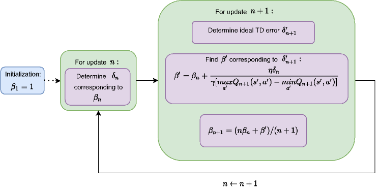
Figure 1: Block diagram describing the processes involved in Balanced $Q-$learning

Proposition 1.

For a transition $(s,a,r,s^{\prime})$ in an MDP $\mathcal{{M}}$, where the $n^{th}$ update of the action value $Q_{n}(s,a)$ conducted as per Equation 1 is associated with a TD error $\delta_{n}$, and the modified target for the $(n+1)^{th}$ update is computed as per Equation 5, with $Q^{*}(s,a)$ being approximated by the balanced target in Equation 2, the equivalent balancing factor $\beta^{\prime}$ for the $(n+1)^{th}$ update is given by

$$\beta^{\prime}=\beta_{n}+\frac{\eta\delta_{n}}{\gamma[\underset{a^{\prime}}{max\thinspace}Q_{n+1}(s^{\prime},a^{\prime})-\underset{a^{\prime}}{min\thinspace}Q_{n+1}(s^{\prime},a^{\prime})]}$$ (6)

where $\eta$ is a step-size hyperparameter, $\gamma$ is the discount factor and $Q_{n+1}$ is the action value estimate corresponding to the $(n+1)^{th}$ update.

Proof.

$Q^{*}(s,a)$ in Equation 5 is initially approximated as $Q_{T_{n}}=r(s,a)+\gamma[\beta_{n}\underset{a^{\prime}}{max}Q_{n}(s^{\prime},a^{\prime})+(1-\beta_{n})\underset{a^{\prime}}{min}Q_{n}(s^{\prime},a^{\prime})]$ using the balancing factor $\beta_{n}$ (Initialized to $1$). Subsequently, Equation 5 can be re-written as:

$$Q_{T_{n+1}}^{\prime}=Q_{T_{n+1}}+\eta[Q_{T_{n}}-Q_{n}(s,a)]$$ (7)

$$=Q_{T_{n+1}}+\eta\delta_{n}$$ (8)

where $\delta_{n}$, the TD error associated with the $n^{th}$ update is:

$$\delta_{n}=r(s,a)+\gamma[\beta_{n}\underset{a^{\prime}}{max}Q_{n}(s^{\prime},a^{\prime})+(1-\beta_{n})\underset{a^{\prime}}{min}Q_{n}(s^{\prime},a^{\prime})]-Q_{n}(s,a)$$ (9)

or

$$\delta_{n}=Q_{T_{n}}-Q_{n}(s,a)$$ (10)

Corresponding to these estimates, the ideal TD error for the subsequent (i.e., $(n+1)^{th}$) update of the state-action pair can be computed analogous to Equation 10 as:

$$\delta^{\prime}_{n+1}=Q^{\prime}_{T_{n+1}}-Q_{n+1}(s,a)$$ (11)

Using Equation 8, the above relation can be expressed as:

$$\delta^{\prime}_{n+1}=Q_{T_{n+1}}+\eta\delta_{n}-Q_{n+1}(s,a)$$ (12)

In addition, with the current estimate of the balancing factor $\beta_{n}$, $Q_{T_{n+1}}$ in the above equation can be further expanded as:

$$Q_{T_{n+1}}=r(s,a)+\gamma[\beta{}_{n}maxQ_{n+1}(s^{\prime},a^{\prime})+(1-\beta_{n})\underset{a^{\prime}}{min}Q_{n+1}(s^{\prime},a^{\prime})]$$

Substituting this in Equation 12, we obtain the ideal TD error associated with the $(n+1)^{th}$ update, as per the current value of balancing factor $\beta_{n}$:

$$\delta^{\prime}_{n+1}=r(s,a)+\gamma[\beta_{n}\underset{a^{\prime}}{max}Q_{n+1}(s^{\prime},a^{\prime})+(1-\beta_{n})\underset{a^{\prime}}{min}Q_{n+1}(s^{\prime},a^{\prime})]+\eta\delta_{n}-Q_{n+1}(s,a)$$ (13)

This TD error $\delta^{\prime}_{n+1}$ can be assumed to be associated with an equivalent balancing factor $\beta^{\prime},$ such that:

$$\delta^{\prime}_{n+1}=r(s,a)+\gamma\left[\beta^{\prime}\underset{a^{\prime}}{max\thinspace}Q_{n+1}(s^{\prime},a^{\prime})+\left[1-\beta^{\prime}\right]\underset{a^{\prime}}{min\thinspace}Q_{n+1}(s^{\prime},a^{\prime})\right]-Q_{n+1}(s,a)$$ (14)

From Equations 13 and 14, we get:

$$\beta^{\prime}=\beta_{n}+\frac{\eta\delta_{n}}{\gamma[\underset{a^{\prime}}{max\thinspace}Q_{n+1}(s^{\prime},a^{\prime})-\underset{a^{\prime}}{min\thinspace}Q_{n+1}(s^{\prime},a^{\prime})]}$$ (15)

∎

Hence, at each step, we use an initial estimate $\beta_{n}$, and compute $\beta^{\prime}$, (clipped to $[0,1]$ if needed; clipping ensures that only realistic targets are used), which is used to compute the balanced target, based on which the action values are updated. The subsequent value of $\beta_{n}$ is also updated online, as explained later.

Interpreting the $\beta^{\prime}$ update: Equation 15 suggests that when $\delta_{n}=0$, an appropriate value of $\beta_{n}$ is being used to determine the balanced target, and thus, $\beta^{\prime}$ assumes the same value as $\beta_{n}$. When $\delta_{n}\neq 0$, the direction of the update depends solely on $\delta_{n}$, as the denominator $[\underset{a^{\prime}}{max\thinspace}Q_{n+1}(s^{\prime},a^{\prime})-\underset{a^{\prime}}{min\thinspace}Q_{n+1}(s^{\prime},a^{\prime})]$ is always positive. $\delta_{n}$, (which can be expressed as $\delta_{n}=Q_{T_{n}}-Q_{n}(s,a)$), when positive, indicates that the estimated action value $Q_{n}(s,a)$ still falls short of the determined balanced target $Q_{T_{n}}$ (which is determined using $\beta_{n}$). Hence, in order to drive up the value of $Q_{n}(s,a)$, $\beta^{\prime}$ is updated to a value larger than $\beta_{n}$, increasing the subsequent update’s reliance on the maximization term. Similarly, when $\delta_{n}$ is negative, it implies that $Q_{n}(s,a)$ exceeds the balanced target $Q_{T_{n}}$. In order to drive down the value of $Q_{n}(s,a)$, $\beta^{\prime}$ is updated to a lower value, increasing its reliance on the minimization term. Hence, $\beta^{\prime}$ makes sample-specific adjustments to the subsequent target in order to drive up or drive down the current action value estimate as required.

Updating $\beta_{n}$: Initialized as $1$, $\beta_{n}$ is subsequently updated as the incremental average of $\beta^{\prime}$ following each action value update:

$$\beta_{n+1}=(n\beta_{n}+\beta^{\prime})/(n+1)$$ (16)

As $\beta_{n}$ controls the general extent of reliance on the best and worst possible estimated future returns for all interactions, it can be interpreted as an estimate of the average degree of optimism for a given environment. This is in contrast to $\beta^{\prime}$, which is a sample-specific degree of optimism. Algorithm 1 summarizes the steps involved in balanced DQN, a DQN variant of balanced $Q-$learning. A tabular version of the algorithm is shown in Appendix C. The process is also pictorially depicted in Figure 1.

Practical considerations: When action values are learned using a DQN-like approach, it is common to update the neural network parameters by sampling batches of transitions (As shown in Algorithm 1). That is, corresponding each batch, a single action value update is carried out. Since the average value of $\beta_{n}$ (Equation 16) is computed as the average value of $\beta^{\prime}$ used over the action-value updates, for each batch, we compute $\beta_{batch}^{\prime}$ as the mean value of $\beta^{\prime}$ corresponding to samples in the batch (and treat this as a representative value for that batch), and use this value to update $\beta_{n}$. Doing so allows $\beta_{n}$ to be computed as the average value of $\beta^{\prime}$ over action-value updates. We treat this as a caveat associated with the DQN-variant of our algorithm.

Algorithm 1 Balanced DQN

1:  Input:

2:  Step sizes $\alpha$, $\eta,$ exploration parameter $\epsilon$, discount factor $\gamma$, maximum number of steps $N_{max}$, Batch size $b$

3:  Initialize replay buffer $D$, count $n=1$, $\beta_{1}=1$ and $Q-$network $Q(s,a,\theta)$

4:  Initialize $Q_{n}$ and $Q_{n+1}$ as $Q(s,a,\theta)$

5:  Get initial state $s$

6:  Output: Learned value function $Q_{N_{max}}$

7:  while $n\leq N_{max}$ do

8:     Use $\epsilon-$greedy strategy to choose action $a$; observe $r,s^{\prime}$

9:     Store transition $(s,a,r,s^{\prime})$ in $D$

10:     Sample mini-batch $B$ of size $b$ from $D$

11:     for $m\in B$ do

12:        Compute TD error $\delta_{n}$ using $Q_{n}$ (Equation 9)$:$

13:        Obtain $\beta^{\prime}_{m}$ for sample $m$ as per Equation 15: $\beta_{m}^{\prime}=\beta_{n}+\frac{\eta\delta_{n}}{\gamma[\underset{a^{\prime}}{max\thinspace}Q_{n+1}(s_{m}^{\prime},a^{\prime})-\underset{a^{\prime}}{min\thinspace}Q_{n+1}(s_{m}^{\prime},a^{\prime})]}$

14:        Clip $\beta_{m}^{\prime}$ to the range $[0,1]$

15:        Compute target

$$Q_{T_{m}}=r_{m}(s_{m},a_{m})+\gamma\beta_{m}^{\prime}\underset{a^{\prime}}{max\thinspace}Q_{n+1}(s_{m}^{\prime},a^{\prime})+(1-\beta_{m}^{\prime})\underset{a^{\prime}}{min\thinspace}Q_{n+1}(s^{\prime}_{m},a^{\prime})]$$

16:     end for

17:     $\beta_{batch}^{\prime}=\frac{1}{b}\underset{i}{\sum}\beta_{i}^{\prime}$

18:     Update $\beta_{n+1}$ as $\beta_{n+1}=(n\beta_{n}+\beta_{batch}^{\prime})/(n+1)$

19:     Store $Q_{n}$ as the current estimate: $Q_{n}\leftarrow Q(s,a;\theta)$

20:     Update network parameter $\theta$ using the computed targets $Q_{T}$: $\theta\thickapprox argmin_{\theta}[Q_{T}-Q(s,a;\theta)]^{2}$

21:     Store $Q_{n+1}$ as the updated estimate: $Q_{n+1}\leftarrow Q(s,a;\theta)$

22:     Update state: $s\leftarrow s^{\prime}$

23:     Update count: $n\leftarrow n+1$

24:  end while

Balanced $Q-$learning can also be shown to converge in tabular environments as long as $\eta\leq\gamma$, in addition to other standard conditions on the step size $\alpha$ (Theorem 2).

Theorem 2.

In a finite MDP ($\mathcal{S,A,T,R}),$ balanced $Q-$learning, given by the update rule:

$$Q_{n+1}(s,a)=Q_{n}(s,a)+\alpha_{n}(s,a)\left[Q_{T}-Q_{n}(s,a)\right]$$

where

$$Q_{T}=r(s,a)+\gamma\left[\beta^{\prime}\underset{a^{\prime}}{max\thinspace}Q_{n}(s^{\prime},a^{\prime})+(1-\beta^{\prime})\underset{a^{\prime}}{min\thinspace}Q(s^{\prime},a^{\prime})\right]$$

converges to a fixed point with probability 1 as long as $\eta\leq\gamma$, $\underset{n=1}{\overset{\infty}{\sum}}\alpha_{n}(s,a)=\infty$ and $\underset{n=1}{\overset{\infty}{\sum}}\alpha_{n}^{2}(s,a)<\infty$ $\forall(s,a)\in\mathcal{S\times\mathcal{A}}$, where $\eta$ is a step size hyperparameter.

Proof.

(Proof of Theorem 2 is provided in Appendix A.2) ∎

We note that due to the ‘min’ operator in the learning target, balanced $Q-$learning converges to a more risk-averse fixed point compared to algorithms such as standard $Q-$learning, where the learning target depends solely on a maximization term. Although this may not be optimal in terms of reward maximization, it aids online learning performance by accounting for high-risk actions in an environment.

5 Experiments

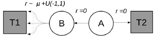
Figure 2: A simple MDP with two non-terminal states $A$ and $B$, and two terminal states $T1$ and $T2$. The transition into $T1$ is associated with a reward $r\sim\mu+U(-1,1)$, where $\mu$ is the mean reward. All other transitions are associated with a reward of $0$. Depending on whether $\mu$ is positive or negative, the optimal action from $A$ is to move either left or right.

In this section, we demonstrate balanced $Q-$learning on a simple MDP (Figure 2), following which we present further empirical comparisons in other environments. We choose DQN[9], double DQN[5], maxmin DQN [6], averaged DQN [7] and REDQ learning [10] as baselines for comparison.

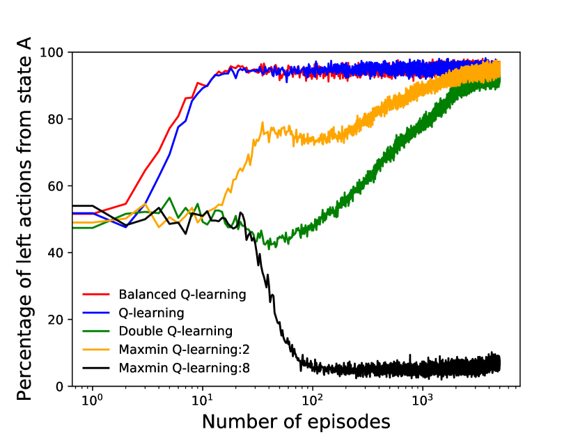
(a) Mean reward $\mu=+0.1$. Higher values are better.

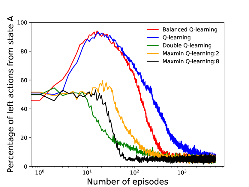
(b) Mean reward $\mu=-0.1$. Lower values are better.

Figure 3: The percentage of left actions taken from state $A$ during training, computed over $500$ trials, for the two reward settings: (a) $\mu=+0.1$ and (b) $\mu=-0.1$.

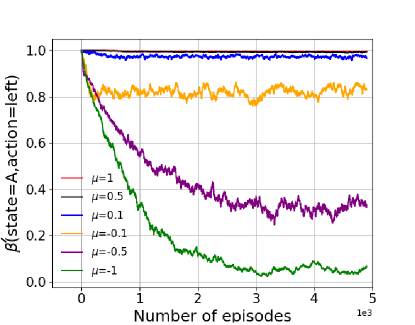
Figure 4: Plot showing the variation of $\beta^{\prime}$ for left actions taken from state A of Figure 2, for different values of mean rewards $\mu$..

Robustness to different bias preference scenarios: Certain learning scenarios could benefit from an inherent overestimation bias, whereas in other scenarios, underestimation may be preferred. Hence, it is undesirable for the underlying learning algorithm to be strictly associated with either of these bias types. The goal of balanced $Q-$learning is to adaptively provide the correct type of biases, depending on the scenario.

We demonstrate this property using a simple MDP shown in Figure 2, previously used to study overestimation issues during learning [2, 6]. It consists of non-terminal states $A$ and $B$, and terminal states $T1$ and $T2$. An episode begins in state $A$, from which the agent can choose between two actions: to move left (towards state $B$) or right (towards state $T2$), both of which return a reward of $0.$ From state $B$, the agent can choose from $8$ different actions, all of which take it to state $T1$, but the reward corresponding to these actions is drawn from a uniform distribution $U(1,-1)$, with mean $\mu$. That is, $r\sim\mu+U(1,-1)$.

Intuitively, if the the mean reward $\mu$ is positive, the action of going left from state $A$ is of relatively high value (and thus benefits from an overestimation bias, as explained in the discussion following Theorem 1), and the optimal policy at state $A$ is to always move left. Similarly, if $\mu$ is negative, the action of moving left from state $A$ is of relatively low-value (benefits from underestimation), and the optimal policy is to always move right, into state $T2$. Corresponding to these settings, we set $\mu$ to be $+0.1$ and $-0.1$, and test the performance of several $Q-$learning variants with balanced $Q-$learning.

In order to evaluate the performance of the different agents, we compute the percentage of instances (over $500$ trials) where left actions were chosen from state $A$ during training. In the reward setting: $\mu=+0.1$ (Figure 3(a)), a higher percentage of left actions is better (ideally, $100\%$). Here, $Q-$learning, inherently associated with an overestimation bias, performs well, whereas algorithms characterised by significant underestimation biases (Double $Q-$learning and Maxmin $Q-$learning ($N=8$) ) perform relatively poorly. Balanced $Q-$learning, initialized with a balancing factor $\beta=1$, performs on par with $Q-$learning.

For the reward setting: $\mu=-0.1$ (Figure 3(b)), a lower percentage of left actions is better (ideally, $0\%$). In this scenario, the overestimation bias associated with $Q-$learning negatively affects its performance, which is characterised by the initial peak in the percentage of left actions (shown in Figure 3 (b)), only recovering to close-to-ideal values around $4000$ episodes. Balanced $Q-$learning also exhibits an initial tendency to overestimate the value of left actions. This is due to the initialization of balancing factor $\beta$ as $1$. However, it self-corrects to a low percentage of left actions within just a few hundred episodes (an order of magnitude faster than $Q-$learning). This self-corrective nature allows balanced $Q-$learning to perform relatively well in both reward settings, showcasing its ability to remain relatively agnostic to the underlying bias preferences of the environment. In contrast, the performance of maxmin $Q-$learning is highly sensitive to the value of $N$ used. Incorrectly setting $N$ could severely affect the learning performance, depending on the environment’s inherent tendency to prefer overestimation or underestimation. This is not the case with balanced $Q-$learning.

The ability of balanced $Q-$learning to remain agnostic to different bias preference scenarios is further demonstrated by creating environments with different values of the mean reward $\mu$, and tracking the $\beta^{\prime}$ value of taking the left action from state $A$ during learning. For environments with a high value of $\mu$, one would expect optimistic updates to be preferred, whereas in environments with low $\mu$, pessimistic updates would be preferred. As depicted in Figure 4, balanced $Q-$learning maintains high values of $\beta^{\prime}$ for environments with high $\mu$, and converges to low values in environments with low $\mu$, thus allowing it to perform well in a range of environments, irrespective of their inherent bias preferences.

Results on Benchmark Environments: We first evaluate the empirical performance of balanced DQN on multiple games from the MinAtar environment [11], which was designed to decouple the representational complexity associated with Atari games [12, 9] from the task of learning useful behaviors. It has been used as a benchmark environment in recent work exploring methods for controlling the estimation bias [6, 13].

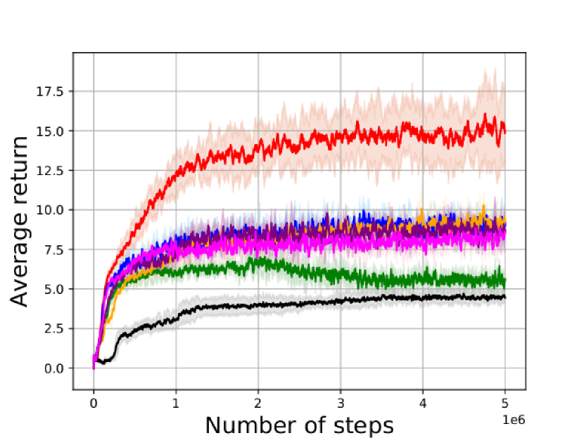
(a) Breakout

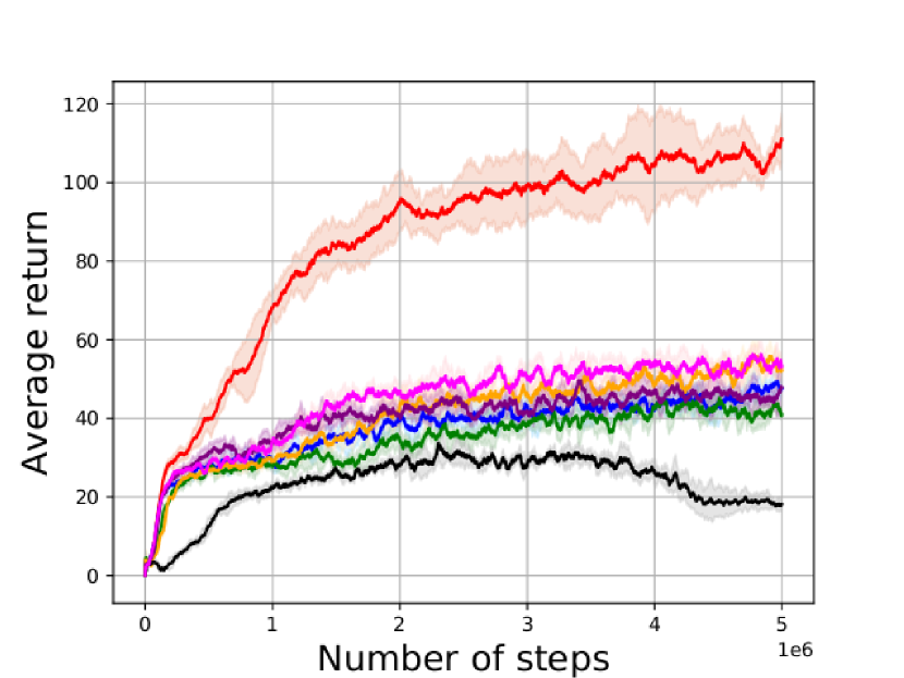
(b) Space Invaders

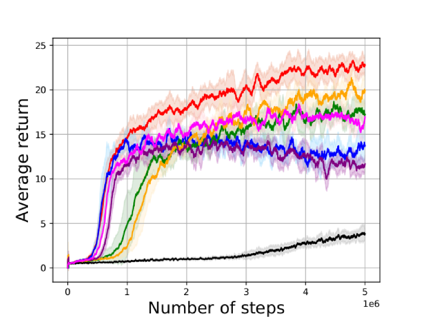
(c) Asterix

Figure 5: Performance plots on the MinAtar environments (a) Breakout, (b) Space Invaders and (c) Asterix. The results are averaged over $10$ runs, and the shaded regions represent standard deviation.

	DQN	Double	Average	RedQ	Maxmin	Balanced
Breakout	8.15±0.61	5.73±0.44	7.86±0.59	7.49±0.55	7.85±0.62	13.02±1.43
Asterix	12.07±1.08	12.18±1.29	11.06±0.90	13.80±0.83	12.80±1.09	17.11±1.21
Space Invaders	37.46±2.39	34.29±2.28	40.02±2.44	44.35±2.30	40.57±1.88	84.95±6.44
Seaquest	11.99±1.87	7.46±1.78	10.56±2.51	9.34±2.03	6.12±1.92	16.33±2.43
Freeway	45.00±0.86	41.99±2.26	44.37±1.01	45.01±0.36	41.34±1.22	45.21±0.56
Island Navigation	30.39±1.45	32.89±1.47	34.57±1.05	24.17±1.12	35.36±0.71	36.17±1.14
CartPole-v0	84.94±8.78	95.20±9.08	110.34±3.66	104.66±4.98	111.02±2.26	106.48±3.64
Tabular Navigation	0.57±0.07	0.47±0.09	-	0.53±0.10	0.05±0.05	0.58±0.08

Table 1: Average rewards (mean±standard deviation) across environments and baselines. Bold represents the highest mean value.

Figure 5 depicts the performance in a subset of the MinAtar environments over $10$ trials. As depicted in Figure 5 and Table 1, balanced DQN exhibits significant performance improvements in almost all the MinAtar games, demonstrating its ability to perform consistently in complex environments. We also consider: a tabular navigation environment [14], Cartpole-v0 from OpenAI gym [15] and the Island Navigation environment [16] to demonstrate the consistency of balanced DQN across different environments. Table 1 demonstrates this consistency, which is unlike other approaches such as maxmin DQN or double DQN, where the performance is highly dependent on the nature of the environment under consideration. Performance curves corresponding to the other environments have been included in Appendix D. For each experiment, we used a step size $\eta=0.2$, which was found to be consistently good across environments (refer Appendix E). The performance of averaged DQN and REDQ learning and maxmin DQN was evaluated using $N=8$ $Q-$networks for target estimation. We also evaluated maxmin DQN at $N=2$. Further details on the hyperparameters used have been specified in Appendix B.

5.1 Balanced $Q-$Learning and Exploration:

From the results thus far, it is evident that Balanced $Q-$learning achieves consistently good performances in multiple environments. As per the intuitions of Lan et al. [6], appropriately biasing an agent would cause it to overexplore high-value regions and underexplore low value regions, leading to an overall improvement in the agent’s performance. Here, we empirically demonstrate that Balanced $Q-$learning exhibits a similar exploratory nature, which could potentially explain its consistently good performance across environments. We consider the cliff world environment [2] shown in Figure 6, where the agent is tasked with navigating from states $S$ to state $G$. Transitions into the ‘Cliff’ and goal regions shown in Figure 6 are terminal, after which the agent is reset to the start position. The ‘Cliff’ region is associated with a highly negative reward of $-100$, whereas all other transitions are associated with a reward of $-1$. Here, the $\epsilon-$greedy exploration takes place with $\epsilon=0.1$, ensuring exploration noise throughout learning. Other hyperparameter settings are set as follows: $\gamma=1$, $\alpha=0.05$ and for balanced $Q-$learning, $\eta=0.2$.

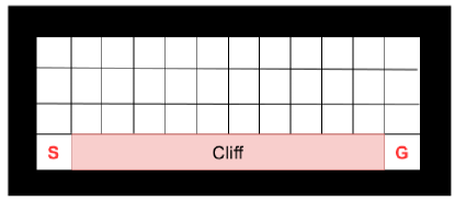
Figure 6: Cliff World environment. The ‘Cliff’ region is associated with $-100$ reward and all other transitions are associated with $-1$ reward.

We compare balanced $Q-$learning with standard $Q-$learning by recording the number of state visits for each state during learning. As depicted in Figure 7, with balanced $Q-$learning, the agent tends to follow more conservative paths, avoiding visiting states very close to the cliff. This is explained by the fact that balanced $Q-$learning tends to undervalue low-reward regions, which prevents excessive exploration into these regions. On the other hand, high-reward regions are overvalued, and the agent encourages exploration into these regions. In contrast to this, standard $Q-$learning simply follows the optimal path, despite the risk of falling into the cliff.

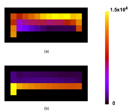
Figure 7: Visitation heat maps for (a) Balanced $Q-$learning and (b) $Q-$learning for the cliff world shown in Figure 6.

6 Related Work

Thrun and Schwartz [3] first reported the issue of systematic overestimation in $Q-$learning, which has since had many proposed solutions. Double $Q-$learning [4] proposed maintaining two independent $Q-$functions, such that the expected action value as per one of them is used to choose the best action for the other. This idea was further extended to the case where $Q-$functions were approximated using neural networks [5]. Although this double network architecture prevents overestimation, it is accompanied by an underestimation bias, which is also potentially harmful. Similar to the double architecture, TD3 [17] also tackled the overestimation problem by maintaining two $Q-$functions, the minimum of which was used to form the targets in the Bellman error loss function.

Recently, maxmin $Q-$learning [6] was proposed as a generalized method to control the estimation bias associated with $Q-$learning. The approach essentially involves maintaining $N$ $Q-$functions, the minimum values of which are used to construct the maximization target. Although maxmin $Q-$learning presents the theoretical possibility of unbiased learning, its performance is highly sensitive to $N$, which must be chosen beforehand. In addition, the bias control is limited to discrete changes in $N$, whereas our approach allows finer control by allowing $\beta$ to assume any real value in the range $[0,1]$. Kuznetsov el al. [18] recently developed an approach for similar finetuned control of overestimation, but in continuous action settings, using multiple critics. Chen et al. [10] also proposed an ensemble approach similar to maxmin $Q-$learning suited to both discrete and continuous action spaces. However, unlike in maxmin $Q-$learning, they leverage high update-to-data ratios, and the learning target is determined on the basis of a subset of all the available networks. Averaged $Q-$learning [7] also determines the $Q-$ learning target using multiple target networks. However, each of the target networks are used to obtain previous estimates, whose average is used as the modified target for $Q-$learning. This enabled the reduction of the variance of the approximation errors of the target, leading to more stable learning.

Zhang et al. [19] proposed an approach to tackle overestimation, using two estimators: one to estimate the maximum expected action value, and the other to estimate the action value. The learning target was expressed as a weighted sum of these estimates. Although our approach shares similarities in the general objective, it maintains a single estimator, and the basis for determining the linear weights is rooted in contextually promoting the right types of biases. In addition, by weighting the optimistic and pessimistic targets, our approach can span the full range of biases. A similar formulation was proposed by Gaskett [20], although only fixed weights were considered. Li and Hou[21] also proposed a similar approach using double estimators, and fixed weights. This limits the applicability of this approach, as it entails foreknowledge of the appropriate weights for a particular environment. In contrast to this, our proposed method dynamically adjusts these weights during learning, raising or lowering it based on an analytically derived update rule. The objective of doing so is to achieve a consistent performance across environments, irrespective of the environment’s tendency to inherently suit a particular type of bias.

7 Conclusion

Depending on the environment and the specific region of the state-action space, both overestimation as well as underestimation bias can potentially aid learning. Through simple derivations, we showed that overestimation aids learning in high-value regions, and underestimation is preferable in low-value regions of the state-action space. We proposed balanced $Q-$learning, a variant of $Q-$learning where the target is constructed using a combination of the maximum and minimum action values of the next state, with the influence of each term being controlled by a balancing factor. We analytically derived a rule for updating this factor online, and showed that the resulting algorithm converges in tabular settings. Through empirical evaluations of the proposed method, we confirmed its robustness to varying reward structures, as well as its ability to consistently achieve a good learning performance in a variety of benchmark environments.

Currently, our approach only considers discrete action settings. Extending the idea of using a balanced target in continuous action spaces remains to be explored. Although we have demonstrated consistently good performances across environments, compared to DQN, we note that our approach requires the storage of two sets of network parameters (one corresponding to update $n$ and the other corresponding to $n+1$). This requirement is however relatively more relaxed in comparison to other ensemble methods, and hence it could constitute a scalable solution to the problem of achieving risk-aware behaviors by controlling the extent of overestimation during learning.

Appendix

Appendix A Proofs

A.1 Proof of Theorem 1

Proof.

Theorem 1 can be proved by induction.

Base Case: $m=1$

Substituting $m=1$ in Equation 4, we get:

$$Q^{*}(s,a)-Q_{n+1}(s,a)=(1-\alpha)\left[Q^{*}(s,a)-Q_{n}(s,a)\right]-\alpha t_{n}(s,a)$$

or

$$Q_{n+1}(s,a)=Q_{n}(s,a)+\alpha\left[Q^{*}(s,a)+t_{n}(s,a)-Q_{n}(s,a)\right]$$

This corresponds to the general TD update equation (Equation 1), where the update target is given by $Q^{*}(s,a)+t_{n}(s,a)$. Denoting $Q_{k}(s,a)$ and $t_{k}(s,a)$ as $Q_{k}$ and $t_{k}$ for brevity, the above equation becomes:

$$Q_{n+1}=Q_{n}+\alpha\left[Q^{*}+t_{n}-Q_{n}\right]$$

Induction Step: $m=k+1$

Assuming Equation 4 is true for $m=k$, we shall prove that it holds for $m=k+1$

From the general TD equation, we get:

$$Q_{n+k+1}=Q_{n+k}+\alpha\left[Q^{*}+t_{n+k}-Q_{n+k}\right]$$

$$Q^{*}-Q_{n+k+1}=Q^{*}-Q_{n+k}-\alpha\left[Q^{*}+t_{n+k}-Q_{n+k}\right]$$

$$Q^{*}-Q_{n+k+1}=(1-\alpha)\left[Q^{*}-Q_{n+k}\right]-\alpha t_{n+k}$$

Substituting the value for $Q^{*}-Q_{n+k},$we get:

$$Q^{*}-Q_{n+k+1}=(1-\alpha)\left[(1-\alpha)^{k}\left[Q^{*}-Q_{n}\right]-\alpha\sum_{i=1}^{k}(1-\alpha)^{i-1}t_{n+k-i}\right]-\alpha t_{n+k}$$

$$Q^{*}-Q_{n+k+1}=(1-\alpha)^{k+1}\left[Q^{*}-Q_{n}\right]-\alpha\left[(1-\alpha)\sum_{i=1}^{k}(1-\alpha)^{i-1}t_{n+k-i}+t_{n+k}\right]$$

$$Q^{*}-Q_{n+k+1}=(1-\alpha)^{k+1}\left[Q^{*}-Q_{n}\right]-\alpha\left[\sum_{i=2}^{k+1}(1-\alpha)^{i-1}t_{n+k-i+1}+t_{n+k}\right]$$

$$Q^{*}-Q_{n+k+1}=(1-\alpha)^{k+1}\left[Q^{*}-Q_{n}\right]-\alpha\sum_{i=1}^{k+1}(1-\alpha)^{i-1}t_{n+k+1-i}$$

∎

This corresponds to Equation 4, with $m=k+1$

A.2 Proof of Theorem 2

Proof.

The convergence of the balanced $Q-$learning is based on the non-expansion property of the term $\beta^{\prime}\underset{a^{\prime}}{max}Q_{n+1}(s^{\prime},a^{\prime})+\left[1-\beta^{\prime}\right]\underset{a^{\prime}}{min}\thinspace Q_{n+1}(s^{\prime},a^{\prime})$ in the update target of balanced $Q-$learning [22].

In order to prove this, we first begin with Equation 15 in the tabular case:

$$\beta^{\prime}=\beta_{n}+\frac{\eta\delta_{n}}{\gamma[\underset{a^{\prime}}{max\thinspace}Q_{n+1}(s^{\prime},a^{\prime})-\underset{a^{\prime}}{min\thinspace}Q_{n+1}(s^{\prime},a^{\prime})]}$$

Using Equation 9 in the above equation, we evaluate the expression $\beta^{\prime}\underset{a^{\prime}}{max}Q_{n+1}(s^{\prime},a^{\prime})+\left[1-\beta^{\prime}\right]\underset{a^{\prime}}{min}\thinspace Q_{n+1}(s^{\prime},a^{\prime})$ to get:

$$=\gamma\beta_{n}[\underset{a^{\prime}}{max\thinspace}Q_{n+1}(s^{\prime},a^{\prime})-\underset{a^{\prime}}{min\thinspace}Q_{n+1}(s^{\prime},a^{\prime})]+\frac{\eta}{\gamma}(r(s,a)-Q_{n}(s,a))+\gamma\underset{a^{\prime}}{min\thinspace}Q_{n+1}(s^{\prime},a^{\prime})\\ \\ +\eta[\underset{a^{\prime}}{\beta_{n}max\thinspace}Q_{n}(s^{\prime},a^{\prime})-(1-\beta_{n})\underset{a^{\prime}}{min\thinspace}Q_{n}(s^{\prime},a^{\prime})]\\$$

In the above expression, $0<\gamma\leq 1$ and $0\leq\beta_{n}\leq 1$. The max and min operators are non-expansions [22], and the term $\frac{\eta}{\gamma}(r(s,a)-Q_{n}(s,a))$ is non expansive as long as $\eta\leq\gamma$. Hence, $\beta^{\prime}\underset{a^{\prime}}{max}Q_{n+1}(s^{\prime},a^{\prime})+\left[1-\beta^{\prime}\right]\underset{a^{\prime}}{min}\thinspace Q_{n+1}(s^{\prime},a^{\prime})$ is a non expansion, which satisfies the convergence criterion [22], under the assumptions $\eta\leq\gamma$, $\underset{n=1}{\overset{\infty}{\sum}}\alpha_{n}(s,a)=\infty$ and $\underset{n=1}{\overset{\infty}{\sum}}\alpha_{n}^{2}(s,a)<\infty$ $\forall(s,a)\in\mathcal{S\times\mathcal{A}}$. ∎

Appendix B Environments and Hyperparameter Settings:

The tabular navigation environment involves an agent in a discrete grid world, tasked with navigating to a predetermined location in the environment. The agent receives a reward of $1$ to reaching the goal location, and $0$ otherwise. CartPole-v0 is a classical control task where the agent is tasked with vertically balancing a pole, hinged on a cart, whose sideways motion can be controlled. Island Navigation is a continuous state navigation environment designed to evaluate the safe exploratory behavior of the agent. Here, the goal is to avoid stepping into ‘water’ locations while navigating to a location in the environment.

In the MinAtar environments, each trial was run for $5e6$ steps, over $10$ trials, with the hyperparameters: batch size=$32$, $\gamma=0.99$, step size= $2.5e-4$ and replay memory size=$1e5$. The exploration parameter $\epsilon$ is initially set to $1$, and decayed linearly over the first $1e5$ steps to a minimum value of $0.1$, after which it was fixed at this value. The target network was updated every $1000$ steps and the optimizer used was RMSprop with gradient clip $5$. In all the MinAtar plots, the average return for a step was obtained by averaging over the previous $100$ episodes. Each MinAtar experiment was performed on an Nvidia Tesla V100 (32GB) GPU, and on average, took about 10 hours per trial per environment.

In tabular navigation, the state of the agent is comprised of its horizontal and vertical positions on the grid, and its goal is to navigate to a specific location. We solved this environment over $15$ trials ($\alpha=0.05$, $\gamma=0.95$ and $\epsilon$ initially set to $1$, linearly decaying to $0$ in the final episode), running it for $1e5$ steps.

For CartPole-v0, we used the following hyperparameter settings: $\alpha=0.001$, $\gamma=0.95$, steps per episode=$200$, total number of steps=$1e4$. $\epsilon$ is initially set to $1$, and decays to a minimum value of $0.01$ as $\epsilon\leftarrow\epsilon\zeta$ after each step, where $\zeta=0.999$. The function approximator is a $2-$ layered feedforward neural network with $24$ nodes per hidden layer, with ReLU activation functions, and trained with a batch size of $32$.

In the Island Navigation environment, we use a $2$ layered feed forward neural network of $100$ nodes each with ReLU activations. The other hyperparameters used are: step size $\alpha=0.001$, $\gamma=0.95$, batch size=$32$, total number of steps=$2e5$. Similar to the cartpole, environment, the initial value of $\epsilon$ is set to $1$, decaying to a minimum value of $0.1$ with $\zeta=0.995$. The optimizer used in Island Navigation and cartpole was Adam [23].

In the simple MDP environment in Figure 2, the hyperparameters used during learning were: $\eta=0.2$, discount factor $\gamma=1$, step size $\alpha=0.01$, and $\epsilon$-greedy exploration with $\epsilon=0.1$. All $Q-$values were initialized with a value of $0$.

In all environments, REDQ learning, Averaged DQN and Maxmin DQN was tested with $N=8$ (number of networks). Maxmin $Q-$learning was also tested with $N=2$. In REDQ learning, we implemented a discrete action version of the algorithm with the size of the subset of networks chosen as $M=5$, and the update-to-data ratio $G=1$.

Appendix C Tabular Implementation:

The tabular implementation of balanced $Q-$learning is shown in Algorithm 2.

Algorithm 2 Tabular implementation of Balanced Q-learning

1:  Input:

2:  Step sizes $\alpha$, $\eta,$ exploration parameter $\epsilon$, discount factor $\gamma$, maximum number of steps $N_{max}$

3:  count $n=1$, $\beta_{1}=1$

4:  Initialize $Q(s,a)$

5:  Initialize $Q_{n}(s,a)$ and $Q_{n+1}(s,a)$ as $Q(s,a)$

6:  Get initial state $s$

7:  Output: Learned value function $Q_{N_{max}}$

8:  while $n\leq N_{max}$ do

9:     Use $\epsilon-$greedy strategy to choose action $a$; observe $r,s^{\prime}$

10:     Compute TD error $\delta_{n}$ using $Q_{n}$ (Equation 9)$:$

11:     Obtain $\beta^{\prime}$ as per Equation 15: $\beta^{\prime}=\beta_{n}+\frac{\eta\delta_{n}}{\gamma[\underset{a^{\prime}}{max\thinspace}Q_{n+1}(s^{\prime},a^{\prime})-\underset{a^{\prime}}{min\thinspace}Q_{n+1}(s^{\prime},a^{\prime})]}$

12:     Clip $\beta^{\prime}$ to the range $[0,1]$

13:     Compute target:

$$Q_{T}=r(s,a)+\gamma[\beta^{\prime}\underset{a^{\prime}}{max\thinspace}Q_{n+1}(s^{\prime},a^{\prime})+(1-\beta^{\prime})\underset{a^{\prime}}{min\thinspace}Q_{n+1}(s^{\prime},a^{\prime})]$$

14:     Update $\beta_{n+1}$ as $\beta_{n+1}=(n\beta_{n}+\beta^{\prime})/(n+1)$

15:     Store $Q_{n}$ as the current estimate: $Q_{n}\leftarrow Q$

16:     Update $Q$ values: $Q(s,a)\leftarrow Q(s,a)+\alpha[Q_{T}-Q(s,a)]$

17:     Store $Q_{n+1}$ as the latest estimate: $Q_{n+1}\leftarrow Q$

18:     Update state: $s\leftarrow s^{\prime}$

19:     Update count: $n\leftarrow n+1$

20:  end while

Appendix D Additional Performance Plots:

Figure 8 shows the performance of Balanced DQN/$Q-$learning in comparison with other baselines, for (a) tabular navigation (b) CartPole-v0 and (c) Island Navigation. Figure 9 shows the performance in MinAtar environments (a) Freeway and (b) Seaquest.

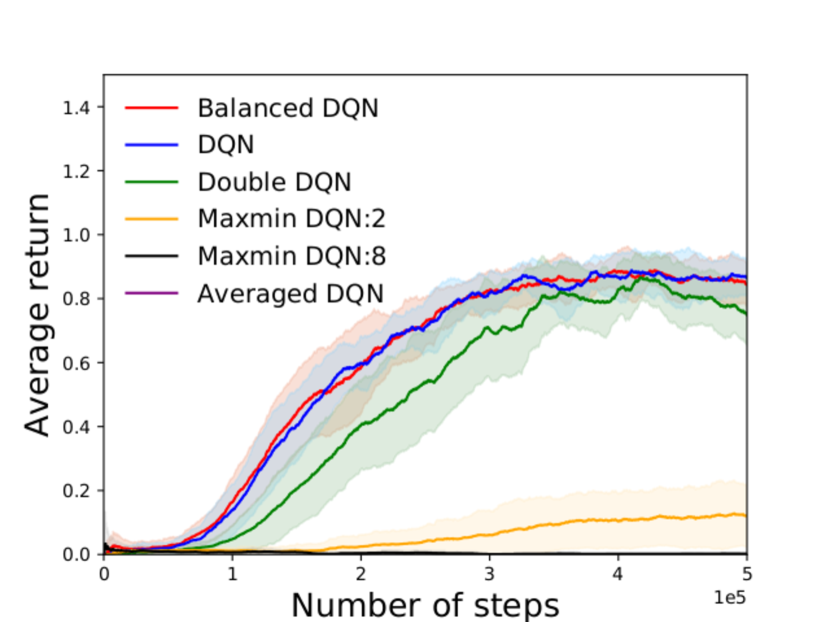
(a) Tabular Navigation

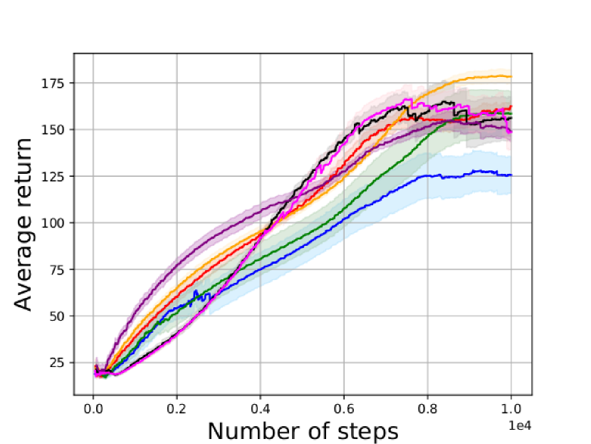
(b) CartPole-v0

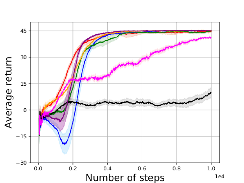
(c) Island Navigation

Figure 8: Performance plots on tabular navigation, CartPole-v0 and Island Navigation environments. The results are averaged over $15$ runs and the shaded regions represent standard deviation.

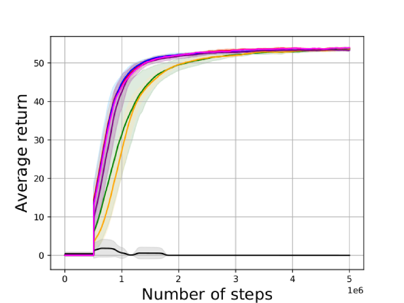
(a) Freeway

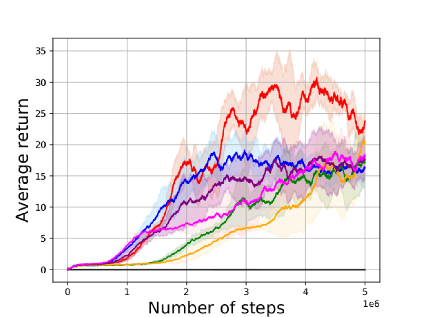
(b) Seaquest

Figure 9: Performance plots on the Seaquest and Freeway MinAtar environments. The results are averaged over $10$ runs and the shaded regions represent standard deviation.

Appendix E Sensitivity of $\eta$

To show the effect of choosing the hyperparameter $\eta$, we repeat the experiments with $\eta$ values of $0.2,0.4,0.6,0.8$ and $1$ in each environment. In each case, the ratio of the total average rewards obtained are plotted relative to the case of $\eta=0$ (which simply corresponds to the case of DQN). As depicted in Figure 10, the agent produces favorable performances for low values of $\eta$ ($\eta>0)$. The performance is unfavorably affected when $\eta$ is set to large values (as is the case when large step sizes are used in general), as this results in large corrections in the TD error. However, as depicted in Figure 10,the algorithm achieves a good performance across a wide range of $\eta$ values.

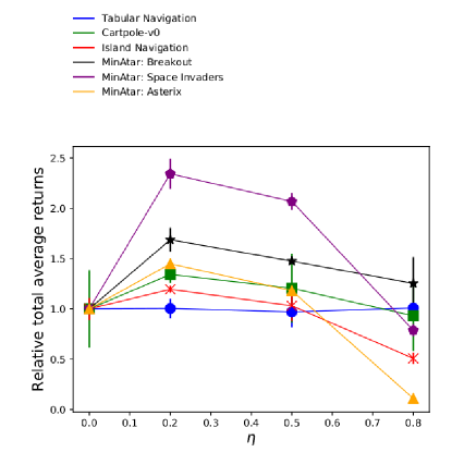
Figure 10: Performance relative to $\eta=0$ (DQN) for different values of $\eta$ in different environments over $3$ runs. The error bars correspond to one standard deviation.

Appendix F Fixed $\beta$

We also examine the effect of fixed values of $\beta$ in contrast to determining $\beta$ online using balanced $Q-$learning. As depicted in Figures 11 and 12, the learning performance is highly sensitive to the specific value of $\beta$ chosen. However, Balanced DQN automatically updates $\beta$ online to the appropriate value.

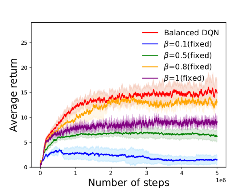
(a) Breakout

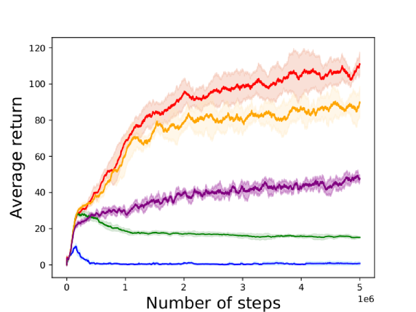
(b) Space Invaders

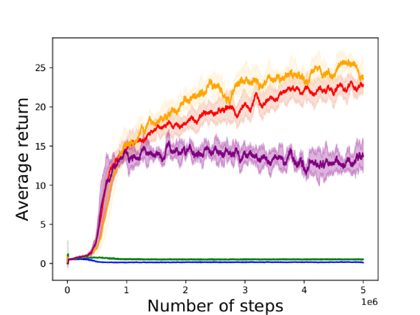
(c) Asterix

Figure 11: Performance plots on the MinAtar environments with fixed $\beta$. The results are averaged over $10$ runs, and the shaded regions represent one standard deviation.

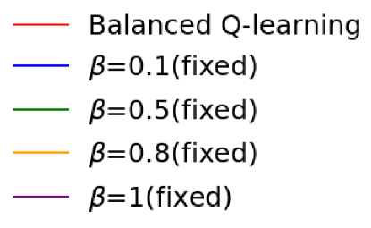
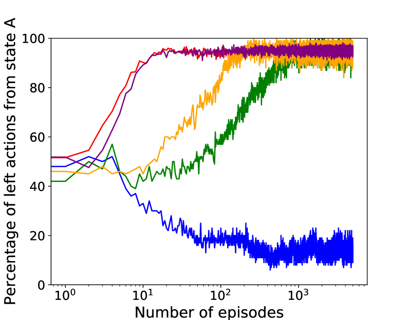
(a) Mean reward $\mu=+0.1$. Higher values are better.

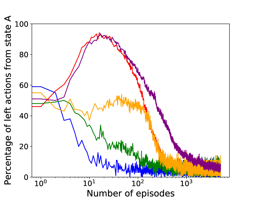
(a) Mean reward $\mu=-0.1$. Lower values are better.

Figure 12: Performance in the simple MDP environment (Figure 2) with fixed $\beta$. The results are averaged over $100$ runs.

References

- [1] C. Watkins, Learningfrom delayed rewards, PhDthesis, Cambridge University, Cambridge, England.
- [2] R. S. Sutton, A. G. Barto, Reinforcement learning: An introduction, Vol. 1, MIT press Cambridge, 1998.
- [3] S. Thrun, A. Schwartz, Issues in using function approximation for reinforcement learning, in: Proceedings of the 1993 Connectionist Models Summer School Hillsdale, NJ. Lawrence Erlbaum, 1993.
- [4] H. V. Hasselt, Double q-learning, in: Advances in neural information processing systems, 2010, pp. 2613–2621.
- [5] H. V. Hasselt, A. Guez, D. Silver, Deep reinforcement learning with double q-learning, in: Thirtieth AAAI conference on artificial intelligence, 2016.
- [6] Q. Lan, Y. Pan, A. Fyshe, M. White, Maxmin q-learning: Controlling the estimation bias of q-learning, in: International Conference on Learning Representations, 2020.
- [7] O. Anschel, N. Baram, N. Shimkin, Averaged-dqn: Variance reduction and stabilization for deep reinforcement learning, in: Proceedings of the 34th International Conference on Machine Learning-Volume 70, JMLR. org, 2017, pp. 176–185.
- [8] M. L. Puterman, Markov Decision Processes: Discrete Stochastic Dynamic Programming, 1st Edition, John Wiley & Sons, Inc., New York, NY, USA, 1994.
- [9] V. Mnih, K. Kavukcuoglu, D. Silver, A. A. Rusu, J. Veness, M. G. Bellemare, A. Graves, M. Riedmiller, A. K. Fidjeland, G. Ostrovski, et al., Human-level control through deep reinforcement learning, Nature 518 (7540) (2015) 529.
- [10] X. Chen, C. Wang, Z. Zhou, K. Ross, Randomized ensembled double q-learning: Learning fast without a model, arXiv preprint arXiv:2101.05982.
- [11] K. Young, T. Tian, Minatar: An atari-inspired testbed for more efficient reinforcement learning experiments, arXiv preprint arXiv:1903.03176.
- [12] M. G. Bellemare, Y. Naddaf, J. Veness, M. Bowling, The arcade learning environment: An evaluation platform for general agents, Journal of Artificial Intelligence Research 47 (2013) 253–279.
- [13] A. Cini, C. D’Eramo, J. Peters, C. Alippi, Deep reinforcement learning with weighted q-learning, arXiv preprint arXiv:2003.09280.
-
[14]
F. Fernández, M. Veloso,
Probabilistic policy reuse
in a reinforcement learning agent, in: Proceedings of the fifth
international joint conference on Autonomous agents and multiagent systems,
ACM, 2006, pp. 720–727.
URL http://dl.acm.org/citation.cfm?id=1160762 - [15] G. Brockman, V. Cheung, L. Pettersson, J. Schneider, J. Schulman, J. Tang, W. Zaremba, Openai gym, arXiv preprint arXiv:1606.01540.
- [16] J. Leike, M. Martic, V. Krakovna, P. A. Ortega, T. Everitt, A. Lefrancq, L. Orseau, S. Legg, Ai safety gridworlds, arXiv preprint arXiv:1711.09883.
- [17] S. Fujimoto, H. Van Hoof, D. Meger, Addressing function approximation error in actor-critic methods, arXiv preprint arXiv:1802.09477.
- [18] A. Kuznetsov, P. Shvechikov, A. Grishin, D. Vetrov, Controlling overestimation bias with truncated mixture of continuous distributional quantile critics, arXiv preprint arXiv:2005.04269.
- [19] Z. Zhang, Z. Pan, M. J. Kochenderfer, Weighted double q-learning., in: IJCAI, 2017, pp. 3455–3461.
- [20] C. Gaskett, Reinforcement learning under circumstances beyond its control.
- [21] Z. Li, X. Hou, Mixing update q-value for deep reinforcement learning, in: 2019 International Joint Conference on Neural Networks (IJCNN), IEEE, 2019, pp. 1–6.
- [22] C. Szepesvari, M. Littman, Generalized markov decision processes: Dynamic-programming and reinforcement-learning algorithms, in: Proceedings of International Conference of Machine Learning, Vol. 96, 1996.
- [23] D. P. Kingma, J. Ba, Adam: A method for stochastic optimization, arXiv preprint arXiv:1412.6980.