J1832.4-1627, the first eclipsing stream-fed intermediate polar

We present a photometric study of the newly discovered eclipsing intermediate polar J183221.56-162724.25 (in short J1832) with an orbital period of 8.87 hr. The system features a box-like deep eclipse with a full width at 50% depth of $1970\pm 2$ s and a large-amplitude coherent pulsation with $P_{\mathrm{obs}}$$\,=\!65.18$ min, which represents either the synodic (beat) period or the spin period of the white dwarf (WD). The period ratio is either $P_{\mathrm{spin}}/P_{\mathrm{orb}}$$\,=\,$0.1091 or 0.1225, respectively. The eclipsed light originates almost entirely from the two accretion spots and columns on the WD, with characteristics indicative of pole flipping. There is no evidence for an accretion disk, and we identify J1832 as the first deeply eclipsing stream-fed intermediate polar. Our $grizy$ photometry in eclipse yielded an $i$-band AB magnitude of the Roche-lobe-filling secondary star of 18.98(3), an extinction $E_{\mathrm{B-V}}$$\,=\!0.54\!\pm\!0.17$, and a spectral type $\sim\,$K6. Dynamic models, fitting the photometry, limit the distance to between 1270 and 2500 pc for masses of the secondary star, $M_{2}$, between 0.16 and 1.0 $M_{\odot}$, well within the Gaia EDR3 confidence limits. Employing a luminosity selection inspired by binary population studies yields a mean $M_{2}\!=\!0.32$ $M_{\odot}$ with a 2$\sigma$ upper limit of 0.60 $M_{\odot}$ and a mean distance $d\!=\!1596$ pc with a 2$\sigma$ upper limit of 1980 pc. The secondary star is located in its Hertzsprung-Russell diagram at a mean $T_{\mathrm{eff,2}}\!=\!4120$ K and log$(L_{2}/L_{\mathrm{\odot}})\!=\!-0.92$, from where the binary can evolve into either a polar or an ultracompact binary with a highly magnetic primary. The system displays a variable accretion rate, lapses repeatedly into short-lived low states of negligible accretion, and currently displays an orbital period that decreases on a timescale of $\tau\!\sim\!3\,\times\!10^{5}$ yr. X-ray observations, optical spectroscopy, and spectropolarimetry have a high potential for studies of the properties of J1832 as an individual object and of stream-fed accretion in general.

1 Introduction

Magnetic cataclysmic variables (CVs) contain an accreting white dwarf (WD) with a surface field strength in the MG regime fed by a low-mass secondary star. They come in two flavors, the synchronized polars (or AM Herculis stars) and the non-synchronized intermediate polars (IPs). Polars lack an accretion disk, and the WD accretes via a quasi-stationary stream that guides the matter from the inner Lagrangian point, $L_{1}$, more or less directly to the WD. In most IPs, on the other hand, the WD accretes via the intermediary of an accretion disk with an inner bound defined by the equality of viscous and magnetic stresses at the radius of the WD’s magnetosphere. The difference reflects the typically larger orbital periods and system dimensions of IPs and, perhaps, the typically lower magnetic moments of their primary stars. An intriguing, yet controversial, idea suggested an evolutionary link between the two, identifying IPs as the progenitors of polars (e.g., King et al., 1985; Hameury et al., 1986; Wickramasinghe et al., 1991; King & Lasota, 1991; Patterson, 1994; Norton et al., 2004, 2008; Southworth et al., 2007). The proposition postulates the existence of non-synchronized counterparts to polars, which synchronize and appear as polars in their further evolution toward shorter orbital periods. An IP, approaching such a scenario, might have a freely spinning WD with a sufficiently strong magnetic moment to avoid the formation of a disk and accrete instead from a stream that alternately feeds its two poles, a situation referred to as pole flipping. Unfortunately, no such IP has yet been found. The process of synchronization has been studied, however, in asynchronously rotating polars that were already synchronized and had temporarily lost synchronism by some event, such as a nova outburst, and are currently re-synchronizing. They display spin and orbital periods that differ by only $\sim\!1$%, which corresponds to the situation in an IP just preceding synchronization. Well-studied cases include V1500 Cyg = Nova Cyg 1975, which seems to have acquired synchronism again after 40 years (Harrison & Campbell, 2016), and the still asynchronous systems BY Cam (Honeycutt & Kafka, 2005), V1432 Aql (Littlefield et al., 2015), and CD Ind (Littlefield et al., 2019). Because of the near equality of spin and orbital periods, the synodic (beat) periods are long, between 7 and about 62 days. As a consequence, the phenomenology of asynchronous polars is generally rather complex, more complex, in fact, than expected for a stream-fed IP that is still far from synchronism.

Despite intense searches, only one secure candidate of a stream-fed IP has so far been discovered, V2400 Oph, which, unfortunately, is not particularly well suited for studying the conjectured IP-polar connection. It is seen at an inclination of only $\sim\!10\degr$, and consequently its system parameters are not well known (Buckley et al., 1995, 1997; Hellier & Beardmore, 2002; Joshi et al., 2019). Other IPs display a mixture of disk-fed and stream-fed accretion, showing pulsations at both the spin and the synodic period that are produced by the phenomenon of stream overflow. Part of the stream that impacts on the outer disk manages to flow over the disk and carry its angular momentum directly into the WD’s magnetosphere (Lubow, 1989). Still others, such as TX Col, usually dominated by disk-fed accretion, show stream-fed intervals after losing and before reestablishing the disk (Littlefield et al., 2021), which is of interest in itself as it allows the process of disk formation to be observed.

Eclipsing systems offer obvious advantages for in-depth studies of the system parameters. They permit reliable measurements of the component masses, allow the usually faint secondary star to be detected in eclipse, and provide insight into the structure of the accretion region because practically the entire surface of the WD comes into view as it rotates. Unfortunately, the number of eclipsing IPs is exceedingly small. Of the 117 IPs and IP candidates in the last version of the Ritter & Kolb (2003) catalog (final online version 7.24, 2016), only four show a deep eclipse. These are, with one addition, the classical systems DQ Her (Nova Her 1934) and XY Ari, V902 Mon=IPHAS J0627 (Aungwerojwit et al., 2012), V597 Pup, the now faint Nova Puppis 2007 (Warner & Woudt, 2009), and Nova Sco 1437 (Potter & Buckley, 2018, and references therein). Alas, all five contain luminous accretion disks.

A feature shared by some IPs and many polars are irregular long-term brightness variations, including states of vanishing accretion, referred to as low states. In the usual high states, the accretion luminosity outshines the stellar components, and, in many systems, the WD becomes detectable only in a low state. By no means do all IPs provide this opportunity. The well-studied 13 mag disk-fed system EX Hya, for example, exhibits rare outbursts but has not lost its bright disk since observations started more than 60 yr ago (see the AAVSO long-term light curve). As a consequence, the properties of both stellar components are still not well known (Eisenbart et al., 2002; Belle et al., 2003; Hoogerwerf et al., 2004; Beuermann & Reinsch, 2008, 2013).

In this paper we present a photometric study of J183221.56-162724.25 (henceforth J1832), the first deeply eclipsing stream-fed IP that has it all: (i) Its orbital period of 8.87 hr and a coherent large-amplitude 65-minute pulsation qualify it as an IP; (ii) it showed no evidence for an accretion disk in three consecutive observing seasons, suggesting that this is a long-lasting feature; (iii) the emitted light, apart from that of the secondary star, originates from the immediate vicinity of the WD, probably the tall accretion columns at both poles; (iv) the entire central region suffers a deep eclipse by the secondary star; (v) ingress and egress are fast and unresolved at our time resolution of about 30 s; (vi) the evidence for pole flipping supports its identification as a stream-fed IP; and (vii) it lapsed repeatedly into low states, offering the prospect for orbital phase-resolved studies of the secondary star and the WD in spectral regions where either one dominates. No object similar to short is currently known.

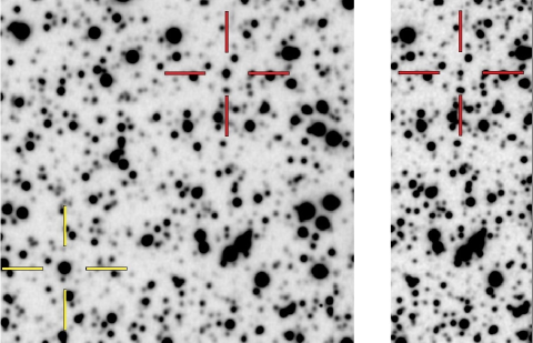
Figure 1: Finding chart for J183221.56-162724.25. The $r$-band images were taken on 12 May 2021 with MuSCAT3 on the FTN. N is up, E to the left, and sizes are 80″$\times$80″ and 30″$\times$80″. The target and the comparison star are indicated by the red and yellow crosses, respectively. The right panel shows the target in the eclipse.

The new IP was discovered on 26 July 2019 by E. Schwab as a side product of the search for the lost comet P/2012 K3 (Gibbs) using the 80 cm Schmidt telescope of the German-Spanish Astronomical Center at Calar Alto (CA), Spain, and described by Schwab & Breitenstein (2019). It received the AAVSO Unique Identifier 000-BNG-512. It was previously (and incorrectly) automatically classified in the Pan-STARRS 3$\pi$ survey (Sesar et al., 2017) as an RR Lyr star. It carries the Gaia Data Release 2 (DR2) identifier 4102856333775127296 and is located at RA,Dec. (2000) 18 32 21.56,$-$16 27 24.2 ($l,b=16\aas@@fstack{\circ}1351,-3\aas@@fstack{\circ}3367$) in the Milky Way (Fig. 1). The Gaia Early Data Release 3 (EDR3) lower and upper confidence limits for the geometric distance are 1254 and 2847 pc, respectively (Bailer-Jones et al., 2021). We present a photometric study of the object, including an analysis of phase-resolved light curves taken in white light (WL) and multicolor $grizy$ light curves taken through the eclipse. The extinction as measured by us is $E_{\mathrm{B-V}}$$\,=\!0.54\!\pm\!0.17$. Measurements of the brightness and spectral type of the secondary star allowed us to restrict the system parameters.

2 Observations

A total of 3551 WL images were taken on 32 nights in 2019, 2020, and 2021 with the 80 cm Schmidt telescope at the CA Observatory, Spain, equipped in 2019 with an SBIG ST 10-XME charge-coupled device camera and in 2020 and 2021 with a Proline PL23042 camera. The 2019 data were described by Schwab & Breitenstein (2019). Here, we summarize the combined results of the 2019, 2020, and 2021 campaigns and report updated ephemerides for the orbital motion and the rotation of the WD. All CA data were taken with a clear filter in WL and exposed for 60 s. Additional long runs in WL were performed with the MONET/South telescope at the Sutherland site of the South African Astronomical Observatory (SAAO). Shorter observations that covered preferentially the eclipse were performed with telescopes of the Las Cumbres Observatory (LCO), namely the 2-meter Faulkes Telescope South (FTS) and the 1-meter telescope at Siding Spring, Australia, the 2-meter Faulkes Telescope North (FTN) at the Haleakala Observatory, Hawaii, and the 1-meter telescope at the McDonald Observatory, Texas, USA. These runs were taken in the $grizy$ filters on the Pan-STARRS1 (P1) system (Tonry et al., 2012) or in WL with exposure times mostly of 40 s. Table 1 provides a log of the observations.

Table 1: Journal of time-resolved photometric observations of J1832.

Telescope	Year	No.	No.	Band	Exp.	Plate	Tel.
		nights	exp		(s)	scale
CA Schmidt	2019	12	1410	WL	60	0.74	(1)
SAAO MONET/S	2019	3	270	WL	90,180	0.37	(2)
LCO FTS	2019	11	138	WL,r	60,90,120	0.30	(3)
LCO 1 m McD	2019	2	19	WL,r	60	0.78	(5)
CA Schmidt	2020	14	1410	WL	60	1.29	(1)
LCO 1 m SS	2020	1	16	r	60	0.78	(6)
LCO FTN,FTS	2020	14	228	grizy	40,60,120	0.30	(4,3)
CA Schmidt	2021	6	731	WL	60	1.29	(1)
LCO FTN,FTS	2021	6	183	griz,WL	40,50,60	0.30	(4,3)
LCO 1 m McD,SS	2021	2	142	WL	20,50	0.78	(5,6)
LCO 1 m CT,SAAO	2021	5	155	g	60	0.78	(7,8)

WL = white light. Plate scale is in ″/pix. See also footnote to Table 3.

Table 2: Mid-eclipse times of J1832.

Cycle	Observed	Calculated	Error	O-C	Tel.
	TDB 240000+	TDB 240000+	(days)	(days)
0	58691.53623	58691.53666	0.00006	-0.00043	(1)
16	58697.44818	58697.44847	0.00007	-0.00029	(1)
89	58724.42085	58724.42113	0.00006	-0.00028	(1)
105	58730.33282	58730.33295	0.00011	-0.00013	(2)
140	58743.26482	58743.26504	0.00009	-0.00022	(2)
197	58764.32580	58764.32588	0.00006	-0.00008	(1)
812	58991.56180	58991.56127	0.00006	0.00052	(1)
831	58998.58187	58998.58155	0.00005	0.00032	(1)
881	59017.05611	59017.05597	0.00008	0.00013	(3)
912	59028.51013	59028.51011	0.00006	0.00002	(1)
913	59028.87975	59028.87960	0.00006	0.00015	(4)
919	59031.09682	59031.09653	0.00014	0.00029	(5)
962	59046.98473	59046.98454	0.00009	0.00019	(4)
970	59049.94079	59049.94044	0.00007	0.00035	(4)
1047	59078.39118	59078.39105	0.00011	0.00012	(1)
1050	59079.49998	59079.49952	0.00006	0.00046	(1)
1105	59099.82179	59099.82138	0.00018	0.00041	(4)
1181	59127.90283	59127.90250	0.00021	0.00033	(5)
1704	59321.14464	59321.14496	0.00007	-0.00032	(4)
1726	59329.27385	59329.27370	0.00018	0.00015	(5)
1746	59336.66327	59336.66347	0.00006	-0.00020	(1)
1763	59342.94466	59342.94477	0.00009	-0.00012	(3)
1766	59344.05304	59344.05324	0.00005	-0.00020	(4)
1773	59346.63959	59346.63966	0.00006	-0.00007	(1)
1774	59347.00911	59347.00915	0.00005	-0.00003	(4)
1800	59356.61574	59356.61585	0.00007	-0.00011	(1)
1842	59372.13429	59372.13436	0.00005	-0.00007	(6)

See footnote to Table 3 for information on the telescopes.

Table 3: Minima of the 65-minute pulsation of J1832.

Cycle	Observed	Calculated	Error	O-C	Tel.
	TDB 240000+	TDB 240000+	(days)	(days)
0	58691.44610	58691.44620	0.00180	-0.00010	(1)
22	58692.44140	58692.44200	0.00120	-0.00060	(1)
23	58692.48820	58692.48726	0.00230	0.00094	(1)
65	58694.38780	58694.38833	0.00120	-0.00053	(1)
66	58694.43610	58694.43360	0.00180	0.00250	(1)
87	58695.38200	58695.38413	0.00340	-0.00213	(1)
88	58695.42850	58695.42939	0.00120	-0.00089	(1)
89	58695.47490	58695.47466	0.00230	0.00024	(1)
110	58696.42290	58696.42519	0.00230	-0.00229	(1)
111	58696.46830	58696.47046	0.00230	-0.00216	(1)
132	58697.42280	58697.42099	0.00230	0.00181	(1)
133	58697.46910	58697.46626	0.00230	0.00284	(1)
529	58715.38840	58715.39064	0.00340	-0.00224	(1)
530	58715.43670	58715.43591	0.00180	0.00079	(1)
531	58715.48490	58715.48117	0.00230	0.00373	(1)
727	58724.35270	58724.35284	0.00180	-0.00014	(1)
728	58724.39620	58724.39810	0.00230	-0.00190	(1)
857	58730.23700	58730.23711	0.00250	-0.00011	(2)
858	58730.28220	58730.28237	0.00250	0.00017	(2)
1123	58742.27660	58742.27723	0.00190	-0.00063	(2)
1124	58742.32310	58742.32249	0.00190	0.00061	(2)
1125	58742.36950	58742.36775	0.00130	0.00175	(2)
1146	58743.31480	58743.31829	0.00360	-0.00349	(2)
1611	58764.36580	58764.36587	0.00230	-0.00007	(1)
1632	58765.31570	58765.31640	0.00180	-0.00070	(1)
1633	58765.36110	58765.36167	0.00230	-0.00056	(1)
6631	58991.58810	58991.58916	0.00180	-0.00106	(1)
6697	58994.57600	58994.57656	0.00140	-0.00056	(1)
6698	58994.62120	58994.62182	0.00180	-0.00062	(1)
6741	58996.56690	58996.56816	0.00140	-0.00126	(1)
6785	58998.56010	58998.55976	0.00140	0.00034	(1)
7292	59021.51070	59021.50840	0.00280	0.00230	(1)
7293	59021.55590	59021.55367	0.00280	0.00223	(1)
7314	59022.50360	59022.50420	0.00140	-0.00060	(1)
7315	59022.54960	59022.54947	0.00140	0.00013	(1)
7336	59023.49970	59023.50000	0.00180	-0.00030	(1)
7337	59023.54270	59023.54527	0.00180	-0.00257	(1)
7402	59026.48670	59026.48740	0.00180	-0.00070	(1)
7403	59026.53190	59026.53267	0.00180	-0.00077	(1)
7404	59026.57790	59026.57793	0.00300	0.00003	(1)
7446	59028.48290	59028.47900	0.00300	0.00390	(1)
7447	59028.53040	59028.52426	0.00300	0.00614	(1)
7448	59028.57410	59028.56953	0.00180	0.00457	(1)
8550	59078.44940	59078.45002	0.00180	-0.00062	(1)
8594	59080.44080	59080.44161	0.00180	-0.00081	(1)
15070	59373.56875	59373.56872	0.00180	0.00003	(1)
16460	59436.48437	59436.48514	0.00180	-0.00076	(1)

(1) CA, 80 cm Schmidt, Calar Alto/Spain, (2) SAAO, MONET / S, 1.2 m, Sutherland/SA, (3) LCO, 2 m FTS, Siding Spring, (4) LCO, 2 m FTN, Hawaii, (5) LCO, 1 m McDonald/Texas, (6) LCO, 1 m Siding Spring, (7) LCO, 1 m Cerro Tololo/Chile, (8) LCO, 1 m SAAO.

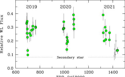
Figure 2: Long-term light curve, showing nightly averages of the WL fluxes relative to comparison star C3 (green dots). The $g$-band fluxes of July 2021 (crosses) are adjusted to approximately match the WL fluxes.

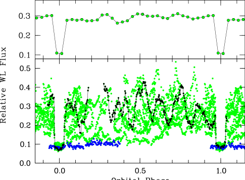
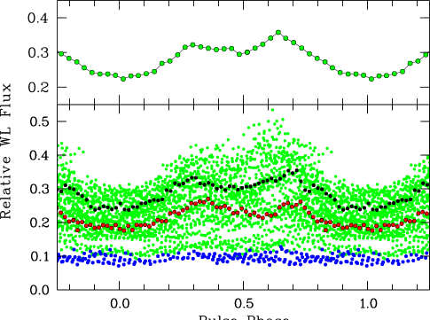
Figure 3: Bottom panels: Light curves in WL folded on the orbital period of Eq. 1 (left) and on the pulse period of Eq. 6 (right). All individual relative WL fluxes are shown as green dots, and selected individual light curves are emphasized in black, red, and blue (see text). Top panels: Mean light curves collected into 32 orbital bins (left) and pulse bins (right).

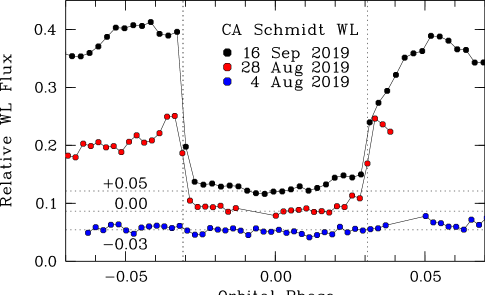
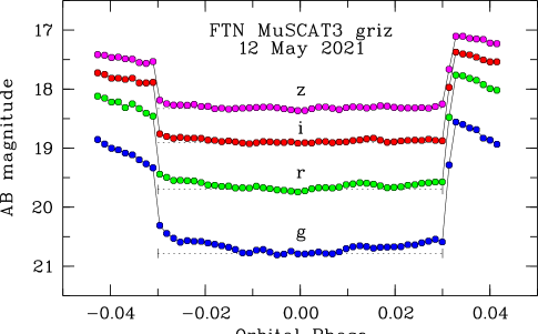
Figure 4: Left: Eclipse light curves in WL, taken with the CA Schmidt telescope, shifted vertically by the indicated amounts. Right: Simultaneous eclipse light curves in the $griz$ filters, taken with the MuSCAT3 photometer on the FTN. The dotted lines indicate the length and flux level of the totality.

All images were corrected for dark current and flat-fielded in the usual way. We performed photometry relative to the comparison star C3, which is located at RA,Dec. (2000) 18 32 24.118, -16 28 08.13, or 57.2″ SE of the target (Fig. 1). It has AB magnitudes on the P1 system $g\!=\!16.933(3),r\!=\!16.357(10),i\!=\!16.107(8),z\!=\!15.931(7)$, and $y\!=\!15.897(7)$. All times were measured in UTC and converted to Barycentric Dynamical Time (TDB), using the tool provided by Eastman et al. (2010) , which accounts also for the leap seconds. As described in Beuermann et al. (2017), the WL measurements at the MONET/S telescope were tied into the standard $griz$ system. For most incident spectra, the WL AB magnitude $w$ is within 0.1 mag of the $r$-band magnitude. We assumed this calibration to be approximately valid also for the CA WL measurements, which is supported by the similar calibration of the P1 $w$-band (Tonry et al., 2012).

The experimental setups of the CA observations were tailored to comet and asteroid searches and not optimized for studies of faint CVs in a dense star field. In particular, the 2020 and 2021 setups with their comparatively large plate scale (Table 1) led to spillover of flux from the near neighbors visible in Fig. 1. The cameras at the MONET/S and the two Faulkes telescopes had more favorable plate scales and for these runs, a spillover problem from the near neighbors at $\sim\!5$″ did not exist. They were still disturbed, however, by at least three faint companions at $\sim\!1$″ separation to the N, E, and S of the target, which required a special effort in the photometric analysis. The southern one is listed in the Gaia EDR3 (Gaia Collaboration, Brown et al., 2021) with $G\!=\!20.82$ at a separation of 1$\aas@@fstack{\prime\prime}$29. In the Gaia high-state measurement, our target had $G\!=\!18.55$ and the influence of the near neighbors was negligible, but in the eclipse they may add noticeably to the measured flux, particularly in the $g$-band, where the secondary star becomes faint. A special effort is, therefore, required for reliable measurements of the eclipse fluxes. Our method makes use of the variability of the target: the difference image of equal exposures outside and inside eclipse lacks all constant sources and contains a clean image of the target in the selected filter. Its relative flux $f_{\mathrm{dif}}$ was measured with respect to comparison star C3, which has the physical flux $F_{\mathrm{C3}}$. We subtracted a fraction $f_{\mathrm{ecl}}$ of the difference image from the eclipse image, such that the result was as best as possible devoid of the target. The target flux in eclipse is then $f_{\mathrm{ecl}}\,f_{\mathrm{dif}}\,F_{\mathrm{C3}}$ and its error is estimated from the uncertainty in establishing $f_{\mathrm{ecl}}$. The method yielded background images in $g,r,i,z,$ and $y$ that contained the near neighbors and illustrated the complexity of the background at this position in the Milky Way.

3 Temporal analysis

3.1 Light curves

The largest body of light curves was taken with the CA Schmidt telescope in WL (Table 1). The source displayed substantial long-term variability as shown in Fig. 2, where the average relative WL fluxes are displayed versus time, supplemented by $g$-band fluxes of July 2021. The “error” bars represent the standard deviations of all individual flux measurements of a given run. The peak-to-peak variations are another factor of about two larger. Most of the time, the source was found at an average WL flux of around 0.30 relative to the comparison star, which we take to represent the high state of the source. In all three observing seasons, the system lapsed into short-lived low or intermediate states of accretion. It was found in a low state on $3-5$ August 2019 (JD 2458700), in an intermediate state between 20 and 27 June 2020 (JD 2459020-9028), and it oscillated between low and intermediate states between 17 July and at least 9 August 2021. Since the source is accreting, we associate these fluctuations with variations in the accretion rate, though not necessarily the mass loss rate from the secondary star.

The two panels of Fig. 3 show the WL measurements of 2019 and 2020 phased on the 8.87 hr orbital period and on the 65-minute pulse period of Eqs. 1 and 6, respectively. All individual flux measurements are displayed as green dots and individual light curves are emphasized by other colors. In the upper parts of both panels, we show the average light curves collected into 32 phase bins. All light curves are characterized by the deep eclipses of the WD by the secondary star and large-amplitude pulsations that we relate to the WD rotation. Examples of the eclipse light curves are shown in Fig. 4. The left panel presents WL light curves at three different accretion levels (note that the zero levels of the ordinate are displaced with respect to each other) and the right one simultaneous high-state $griz$ light curves. The remnant flux at the center of the eclipse is independent of the accretion level and reaches down to that of the secondary star at the center of the eclipse (Sects. 4.1 and 5.5). We can, therefore, exclude a grazing or partial eclipse as in EX Hya (Beuermann & Osborne, 1988; Rosen et al., 1988; Allan et al., 1998). The WD itself is faint compared with the accretion spots and columns, as evidenced by the light curve of 4 August 2019, when the system was caught in a state, when accretion had dropped to a trickle and the eclipse had practically vanished (Figs. 3 and 4, blue dots, and Sect. 4.2). Examples of the large-amplitude pulsations are shown in Fig. 3. The light curve in the left panel (black dots) was pieced together from four individual runs to illustrate the magnitude of the effect.

The rotational light curves in Fig. 3 show that the pulse maxima are more or less double-peaked and the mean rotational light curve in the upper right-hand panel suggests that this is a permanent feature of J1832. Transient double peaks were observed in the photometric light curves of V2400 Oph and V1062 Tau as well (Buckley et al., 1995; Lipkin et al., 2004). Permanent double peaks are naturally produced in pole-flipping stream-fed accretors, as demonstrated by the model calculations of Ferrario & Wickramasinghe (1999, their Fig. 3).

3.2 Is there an accretion disk?

The mean orbital light curve in the left panel of Fig. 3 is essentially flat, with the remnant modulation related to individual 65-minute pulsations. In particular, it lacks the orbital hump expected if there were a viscous disk with a locally puffed-up bulge. Furthermore, the eclipse profile in Fig. 4 lacks disk characteristics as the wide rounded-off component observed in IPHAS J0627 (Aungwerojwit et al., 2012) or the V-shaped eclipse of KIC 5608384 (Yu et al., 2019). Any disk component is, furthermore, limited to stay below the minima of the spin modulation. At our moderate temporal resolution, the transitions into and out of eclipse stay largely unresolved. For the large body of CA WL observations with exposure times of 60 s, the formal average of the fitted transition times between the contact points is $t_{\mathrm{ine}}\!=\!80\pm 56$ s. For the best-resolved of our observations with 20 s exposure and 9 s readout, the transition still occurs within one or two time bin. This corresponds to a lateral extent in the orbital plane of $2\pi\,a\,t_{\mathrm{ine}}/P_{\mathrm{orb}}\!\la\!10^{9}$ cm. While this is entirely consistent with the extent of the accretion columns discussed in Sect. 3.3, even a minimal disk is more than ten times larger. Its diameter would exceed two times the corotation radius where $q\!=\!M_{2}/M_{1}\!\sim\!0.5$ was used for the mass ratio, $P_{\mathrm{orb}}$ is the orbital period, and we used the observed pulse period in lieu of the spin period $P_{\mathrm{spin}}$. Hence, a luminous disk cannot hide in the rapid transitions in J1832.

We now consider the sagging flux profile in the eclipses displayed in Fig. 4. The decreasing flux in the first third and the increasing flux in the last third of the eclipse indicate that an extended source exists that suffers a delayed or incomplete eclipse. In the WL light curve of 16 September 2019, 92% of the eclipsed flux at ingress disappear within a minute and the remaining 8% (until eclipse center) within the next 15 min. In the $r$-band light curve of 12 May 2021, 3% of the eclipsed flux reappear between eclipse center and the end of totality and the remaining 97% within the final minute. Hence, in WL or $r$, a few percent of the total high-state flux are contributed by the extended source. The MuSCAT3 simultaneous $griz$-observations in the right panel of Fig. 4 suggest that this component is rather blue. Our nonsimultaneous observations show that it is highly variable, in particular in the $g$-band. It seems plausible to assign this emission to the outer part of the magnetically guided and likely optically thin accretion stream or to the ballistic stream between $L_{1}$ and its impact on the magnetosphere, which are both prone to a partial eclipse. For the quoted corotation radius, the stream rises to $\sim\!1.5\,\times\!10^{10}$ cm above the orbital plane, sufficient for a time-dependent fraction of the stream to escape eclipse (see also Sect. 5.5). Such a component was seen in other magnetic CVs as well: the long-period IP V902 Mon showed H$\alpha$ emission that did not completely disappear in eclipse (Worpel et al., 2018), and so did the long-period CV KIC 5608384 (Yu et al., 2019), and the polar HY Eri (Beuermann et al., 2017). Hence, emission from the accretion stream far away from the WD is a natural candidate for the variable flux of J1832 in eclipse. Alternatively, we cannot exclude that a minimal faint disk or a ring of matter, circulating the WD near $r_{\mathrm{co}}$ (King, 1993; King & Wynn, 1999; Norton et al., 2008), contributes a few percent to the optical flux.

A final argument against the presence of a viscous accretion disk follows from the low-state observation of $3-5$ August 2019. On 4 August (blue light curve in the left panel of Fig. 4) a viscous disk was absent. Had it been present on 1 August 2019, when the source was still bright, it would have had to have disappeared within 2 days, which is hard to reconcile with the viscous timescale $t_{\mathrm{visc}}\!\sim\!R^{2}/(\alpha Hc_{\mathrm{s}})\!\ga\!20$ d for $R\!>\,$$r_{\mathrm{co}}$, a relative disk height $H/R\!\la\!0.02$, a sound speed of 10 km/s, and a Shakura-Sunyaev parameter $\alpha\!<\!1$. In summary, we conclude that J1832 lacks a viscous accretion disk.

3.3 Orbital period and ephemeris

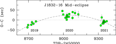
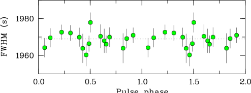
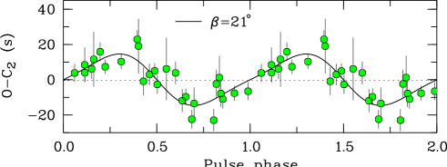
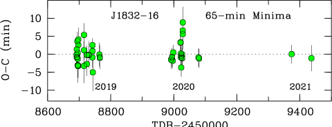
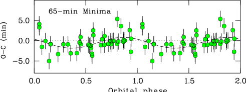
Figure 5: Top: $O-C$ diagram of the mid-eclipse times relative to the linear ephemeris of Eq. 1. The difference between the quadratic and linear ephemerides of Eqs. 2 and 1 is shown as the dashed curve. Second from top: FWHM of the eclipse vs. pulse phase from Eq. 6. Center: $O-C$ values of the mid-eclipse times relative to the quadratic ephemeris vs. pulse phase. The model curve is from Eq. 4 (see text). Second from bottom: $O-C$ diagram for the minimum times of the 65-minute pulsations relative to the linear ephemeris of Eq. 6. Bottom: $O-C$ values of the previous graph vs. orbital phase (see text).

We fitted the ingress into or the egress from eclipse by an analytical model of the occultation of a circular disk of uniform surface brightness by an opaque secondary star. For a given individual exposure, the model value was represented by a Simpson integral of the time-dependent model flux over the finite exposure time, which provides an optimal description of the poorly resolved transitions. The fit parameters for either ingress or egress were (i) the flux before the transition, (ii) the flux after the transition, (iii) the time, at which 50% of the depth is reached, (iv) the duration of the transition between the contact points, (v) the slopes of the time-dependent flux before the transition, and (vi) the slope after the transition. Additional parameters account, as far as possible, for a systematic variation in the atmospheric conditions, for example, an air-mass-dependent transmission. The mid-eclipse time was calculated as the mean of the two times that mark the 50% points at egress and ingress, and the full width at half maximum (FWHM) or duration of the eclipse as their difference. The light curves in Fig. 3 show that the steps in flux and the slopes may differ substantially between ingress and egress, depending on the respective phase in the 65-minute pulsation. It also illustrates the need to include the slopes of the time-dependent fluxes into the fit. The derived mid-eclipse times and the $O-C$ values relative to a linear ephemeris are listed in Table 2 and the $O-C$ values are shown in the top panel of Fig. 5. The alias-free linear ephemeris for all data is

$$T_{\mathrm{ecl,1}}\leavevmode\nobreak\ =\leavevmode\nobreak\ \mathrm{TDB}\leavevmode\nobreak\ 2458691.53666(3)+0.36948844(2)\,E.\leavevmode\nobreak\ \leavevmode\nobreak\ \leavevmode\nobreak\$$ (1)

with $\chi^{2}=387.8$ for 25 dof (degrees of freedom) and 1$\sigma$ errors in the last digits quoted in brackets. Fitting a quadratic ephemeris to all data gives

$$T_{\mathrm{ecl,2}} = \mathrm{TDB}\leavevmode\nobreak\ 2458691.53630(2)+0.36948972(1)\,E$$ (2)

$$\hskip 99.58464pt-\,6.5(1)\,\times\!10^{-10}\,E^{2},$$

with $\chi^{2}\!=\!97.2$ for 24 dof, which is still not good. The difference between the two fits of Eqs. 2 and 1, $T_{\mathrm{ecl,2}}-T_{\mathrm{ecl,1}}$, is shown as the dashed curve in the top panel of Fig. 5. From Eq. 2, the period derivative is $\dot{P}_{\mathrm{orb}}\!=\!-3.5\,\times\!10^{-9}$ s s^-1. Taken at face value, this implies a current period decrease of 0.11 s per year and a timescale of the variation of $3\,\times\!10^{5}$ yr, about two orders of magnitude faster than that predicted by nuclear evolution (e.g., Kalomeni et al., 2016).

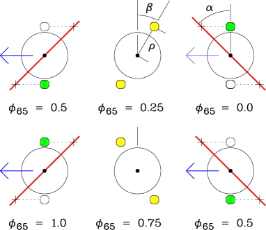
Figure 6: Schematic sketch of the two-pole accreting WD passing the limb of the secondary star, inclined by an angle $\alpha$ to the vertical (red line). The emission regions are located at radial distance $\rho$ and displaced by an angle $\beta$ from the rotational axis. They are indicated by circles, color-coded for their relative brightness: maximal (green), intermediate (yellow), and minimal (open). The projected views are shown for pulse phase at the center of the eclipse, $\phi_{\mathrm{65,c}}$$\,=\!0.25$ (top) and $0.75$ (bottom). The pictures refer to the ingress (right), mid-eclipse (center), and egress (left). The transit takes almost exactly one half of the observed pulse period. The blue arrows indicate the motion of the WD.

3.4 Evidence for pole flipping

Accounting for a period change improves the fit to the mid-eclipse times, but with $\chi^{2}_{\nu}\!=\!4.05$, Eq. 2 still fails to represent the eclipse times well. We searched for a further dependence and found that the mid-eclipse times varied quasi-sinusoidally with the 65-minute pulse phase $\phi_{\mathrm{65,c}}$ measured at the center of the eclipse (Fig. 5, center panel). A sine fit, $\Delta\,T_{\mathrm{ecl}}\!=\!A\,\mathrm{sin}(\varphi_{\mathrm{c}}-\varphi_{0})-\gamma$, gave an amplitude $A\!=\!13.6\pm 1.6$ s, a zero-crossing at $\phi_{0}\!=\!0.03\pm 0.02$, and $\gamma\,=\!-0.5\pm 1.1$ s, with $\chi^{2}\!=\!25.9$ for 24 dof. For brevity, we use here the phase angle $\varphi_{\mathrm{c}}$ at the center of eclipse instead of $2\pi\phi_{\mathrm{65,c}}$. The final model of Eq. 4 below, depicted in the center panel Fig. 5 center, provided a small improvement over the sine fit with $\chi^{2}\!=\!24.0$ for 23 dof. No modulation similar to that of the mid-eclipse times is seen in the FWHM or duration of the eclipse (Fig. 5, second panel from top). The weighted mean FWHM of 17 completely covered eclipses is $1970$ s with a standard deviation of the distribution of 2 s. The pulsations are discussed in Sect. 3.5, their ephemeris is provided in Eq. 6, and its zero point is defined as the pulse minimum.

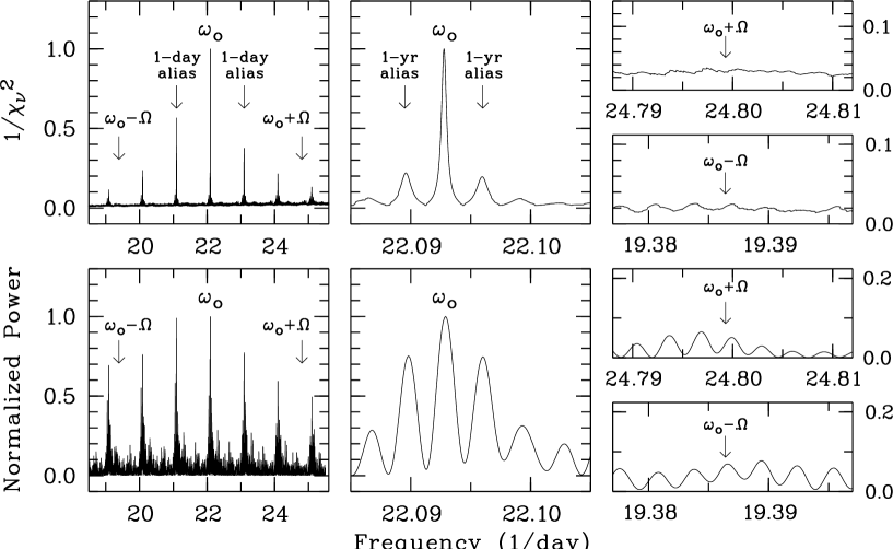
Figure 7: Top: Periodograms for the minimum times of the 65-minute pulsations. The scale on the left also applies to the center panels. Bottom: Lomb-Scargle power spectra for the high- and intermediate-state pulsations outside the eclipse, normalized to a peak value of unity.

The shifts of the mid-eclipse times follow naturally in an IP model with pole flipping that features two accretion columns with brightness varying in antiphase. For simplicity, we adopted sinusoidal variations and represented the columns as point sources that are located at the centroid of the emission at a radial distance $\rho\!>$ $R_{\mathrm{wd}}$ and an angular offset $\beta$ from the rotational axis (Fig. 6). They are eclipsed by the limb of the secondary star that is modeled as a straight edge inclined by an angle $\alpha$ against the vertical (the preferred dynamic models in Sect. 5 have $\alpha$ = 47° or 53°). Special about J1832 is the near equality of the FWHM of the eclipse (1970 s) with one half of the observed 65-minute pulse period (1955 s), implying that the phase angles at ingress and egress are related by $\varphi_{\mathrm{i}}\simeq\varphi_{\mathrm{c}}-\pi/2$ and $\varphi_{\mathrm{e}}\simeq\varphi_{\mathrm{c}}+\pi/2$, respectively. We assumed that the brightness of the sources near both poles varied as $f_{1}\!=\!1+a_{1}\,\mathrm{cos}\,\varphi$ for the upper pole and $f_{2}\!=\!1-a_{2}\,\mathrm{cos}\,\varphi$ for the lower one. With $a_{2}\!>\!a_{1}$, the pulse maximum occurs at $\varphi\!=\!\pi$ or $\phi_{\mathrm{65}}$$\,=\!0.5$ and is dominated by the lower pole. The phasing is as observed (Fig. 3 and Eq. 6) and the preference of the lower pole is adapted from the accretion geometry of EX Hya (Beuermann & Osborne, 1988; Rosen et al., 1988; Allan et al., 1998). Both poles display their maximal brightness difference at ingress and egress for central phases of 0.25 and 0.75 (Fig. 6, green = maximum, yellow = intermediate, open = minimum). For central phases $\phi_{\mathrm{65,c}}$=0 or 0.50, on the other hand, ingress and egress occur at $\phi_{\mathrm{65}}$=0.25 or 0.75 with both poles at intermediate brightness. The dotted lines in Fig. 6 denote the displacements from the limb and the time shifts of ingress and egress relative to that experienced by the center of the WD. The time shifts at both poles are formally the same and differ only by their sign,

$$\Delta t=\pm(\rho/\upsilon)(\mathrm{cos}\,\beta\,\mathrm{tan}\,\alpha+\mathrm{sin}\,\beta\,\mathrm{sin}\,\varphi),$$ (3)

with $\varphi$ the current phase angle and $\upsilon$ the orbital speed of the WD relative to the secondary star. We estimated the combined effect $\Delta\,T_{\mathrm{ecl}}$ on the mid-eclipse time by averaging the four contributions flux-weighted with $f_{1}$ and $f_{2}$. Similarly, we estimated the FWHM as the difference of the weighted mean contributions at egress and ingress. Our simple model predicts that the FWHM does not vary with $\varphi_{\mathrm{c}}$, but that substantial shifts of the mid-eclipse times occur,

$$\Delta\,T_{\mathrm{ecl}}=A\,[\mathrm{cos}\,\beta\,\mathrm{tan}\,\alpha\,\mathrm{sin}\varphi_{\mathrm{c}}-(1/2)\mathrm{sin}\,\beta\,\mathrm{sin}(2\varphi_{\mathrm{c}})],\\$$ (4)

with an amplitude $A\!=\!(a_{1}\!+\!a_{2})\rho/2\upsilon$. The observed dependence of $\Delta T_{\mathrm{ecl}}$ on $\varphi_{\mathrm{c}}$ (or $\phi_{\mathrm{65}}$) in the center panel of Fig. 5 is only moderately skewed, suggesting that the first term in Eq. 4 dominates. We fitted this model to the observed time shifts and obtained $\beta=21\!\pm 10$°, an amplitude $A\!=\!(a_{1}\!+\!a_{2})\rho/2\upsilon\!=\!(12.2\!\pm\!1.4)$ s for $\alpha\!=\!50$° and $\chi^{2}\!=\!24.0$ for 23 dof, as quoted already above. With these parameters, Eq. 4 becomes

$$\Delta\,T_{\mathrm{ecl}}=0\aas@@fstack{d}00016(2)\,[\mathrm{sin}\varphi_{\mathrm{c}}-0.16\,\mathrm{sin}(2\varphi_{\mathrm{c}})],\\$$ (5)

with an amplitude of 14 s and $\varphi_{\mathrm{c}}\!=\!2\pi\phi_{\mathrm{65,c}}$ defined by Eq. 6, below. For $\beta>40$°, the model curve becomes excessively skewed and develops double humps. The amplitudes $a_{1}\!\simeq\!0.2$ and $a_{2}\!\simeq\!0.8$ fit the observed mean 65-min light curve in Fig. 3. The orbital speed is $\upsilon\!\simeq\!3.1\,\times\!10^{7}$ cm s^-1 for a binary separation $a\!\simeq\!1.6\,\times\!10^{11}$ cm (Sect. 5) and the characteristic size of the columns is a plausible $\rho\!\simeq\!10^{9}$ cm, similar to the value estimated by Siegel et al. (1989) for EX Hya. Correcting the original mid-eclipse times for the shifts defined by Eq. 4, linear ephemerides for the individual years gave period differences for 2019 and 2021 relative to 2020 of $+(94\pm 39)$ ms and $-(95\pm 52)$ ms, respectively. A complete orbital ephemeris, given by the addition of Eqs. 2 and 5, requires knowledge of the pulse phase.

The subsequent eclipses of both poles are expected to lead to a phase-dependent structure of the ingress and egress light curves that stayed unresolved in our data, but may provide insight into the accretion geometry, if measured with higher time resolution. We emphasize that such a study was not previously possible, because no deeply eclipsing stream-fed IP was known.

Our simple model of Eq. 4 does not account for more complex geometrical effects and radiative transfer in the emission regions. Consequently, it does not account for variations in the pulse profile as a function of orbital phase. Such variations are predicted, however, in the more elaborate model of Ferrario & Wickramasinghe (1999) for a stream-fed IP accreting alternately at two opposite poles. The model light curves presented in their Fig. 4, feature double-peaked pulses of the line emission and the optical continuum from the extended accretion columns, while the X-ray pulses are single-peaked, because of the two accretion spots on the WD only one is visible at any given instant. The optical pulses display phase shifts over the orbital period and a variation in the separation of the double peaks, including a short single-peaked interval. We measured the minimum times of the continuum flux from Fig. 4 in Ferrario & Wickramasinghe (1999) and found that they display a quasi-sinusoidal variation over the orbit. Such a variation is also observed in our data and shown in the bottom panel of Fig. 5. The amplitude of a fitted sinusoid is $-1.5\!\pm\!0.5$ min (where we have excluded the three outlying minimum times of 2020 in the second panel from the bottom, which show no phase preference). We searched for an orbital variation in the pulse shape in our WL data by sorting all individual WL measurements into an image of $15\times 15$ orbital and pulsational phase bins (not shown). In that image, the shifting pulse minimum is even more clearly visible than in the bottom panel of Fig. 5. In addition, there is an indication that the separation of the two peaks varies over the orbit including what may be a short interval with a central single peak near orbital phase $\phi\!=\!0.5$. Given improved observations, dedicated modeling may be rewarding. Presently, our findings strongly suggest that pole-flipping occurs in J1832, supporting its classification as a stream-fed IP.

Finally, we caution against prematurely identifying the $O-C$ variation in the top panel of Fig. 5 and the quoted period differences between the individual years as real variations in the orbital period before the dynamics of the system is fully understood. Orbital period changes in close binaries, mostly detached ones, are ubiquitous and not well understood. Neither the concept of a third body in the system nor varieties of the Applegate mechanism (Applegate, 1992; Völschow et al., 2018; Lanza, 2020) have so far led to a generally accepted explanation of the observed variations.

3.5 Pulse period and ephemeris

We employed two methods to determine the period of the pulsation: (i) calculating a Lomb-Scargle power spectrum in the MIDAS-TSA context and (ii) subjecting the minimum times of the pulsations to a period search. The former uses the entire information from the rather complex pulse profile, the latter only the reduced information of a well-defined feature with a lower internal scatter. The times of the minima were determined graphically by the bisected-chord technique, marking the center between descent into and ascent from minimum at different flux levels and extrapolating these times to the flux at the minimum. The standard deviation of the distribution of the $O-C$ values of the 47 minima of Table 3 around a linear fit is 2.9 min. For comparison, locating an individual maximum may prove complicated and the uncertainty may exceed 10 min or more. Consequently, the Lomb-Scargle periodogram is expected to be less efficient in measuring the pulse period, but is free of the necessarily somewhat subjective procedure of defining the minima.

The Lomb-Scargle power spectrum for the 2019–2021 high- and intermediate-state observations outside the eclipse, is displayed in the lower left panel of Fig. 7, normalized to a peak value of unity. Maximum power is attained at an observed frequency of the pulsation $\omega_{\mathrm{o}}\!=\!22.09$ day^-1, closely followed by the 1-day alias at 21.09 day^-1. The center bottom panel shows that at higher resolution power appears also at the 1-year alias frequencies separated from the best value by 0.003 day^-1, reflecting the separation of the 2019 and 2020 observing periods by about 320 days. The two right-hand panels demonstrate that there is no power at the side bands $\omega_{\mathrm{o}}\!\pm\!\Omega$, where $\Omega\!=\!2.70644(1)$ day^-1 is the orbital frequency. The same holds for the side band at $\omega_{\mathrm{o}}\!-\!2\Omega$ (Warner, 1986) and is true also for the corresponding side bands that belong to the alias at $\omega_{\mathrm{o}}\,=\!21.09$ day^-1. Not surprisingly, in view of the double peaks, there is significant power at the second harmonics of observed pulse frequency $\omega_{\mathrm{o}}$ and its alias frequencies (not shown). Gratifyingly, the periodogram yields the same frequencies as the Lomb-Scargle power spectrum, but more clearly prefers $\omega_{\mathrm{o}}\!=\!22.09$ day^-1 with a nominal reduced $\chi^{2}_{\nu}$ of unity over 21.09 day^-1 with $\chi^{2}_{\nu}\!=\!1.77$. Again, no signal is detected at any of the side bands of $\omega_{\mathrm{o}}$. Its best value is $\omega_{\mathrm{o}}\!=\!22.09281(4)$ day^-1. In case of the 1-day alias, the fit selects also a different of the 1-year alias frequencies and the best value would become $\omega\!=\!21.090$ day^-1. We consider $\omega_{\mathrm{o}}\!=\!22.09281$ day^-1 as the most probable choice. The analysis of the 47 minimum times in Table 3 yielded the linear ephemeris

$$T_{\mathrm{min}}\!=\!\mathrm{TDB}\leavevmode\nobreak\ 2458691.4462(4)+0.04526359(7)\,E.\leavevmode\nobreak\ \leavevmode\nobreak\ \leavevmode\nobreak\$$ (6)

The best period is $P_{\mathrm{o}}\!=\!3910.774(6)$ s$\,=\!65.1796(1)$ min and the $O-C$ diagram is shown in the second panel from below in Fig. 5. Fitting the minimum times of 2019 and 2020 individually gave periods of 65.1798(10) min and 65.1806(14) min, respectively. There is no evidence for a period variation so far and we accept the pulsation in J1832 as a stable coherent signal. We cannot presently identify the observed period uniquely with either the spin period or the synodic (beat) period of the WD. For the two cases, the spin period is either $P_{\mathrm{spin}}\!=\!3910.775(7)$ s or 3483.976(7) s and the ratio of spin versus orbital periods is $P_{\mathrm{spin}}/P_{\mathrm{orb}}$$\,=\!0.1225$ or 0.1091, respectively.

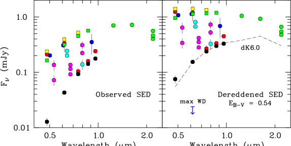
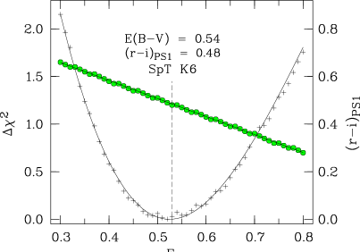
Figure 8: Left: Observed SED of J1832. Black dots refer to the minimum fluxes in the eclipse and represent our best estimate of the SED of the secondary star. Green and yellow squares indicate the SED outside eclipse measured simultaneously with the MuSCAT3 photometer and the FTN on 9 May and 15 April 2021, respectively. Colored dots indicate nonsimultaneous out-of-eclipse fluxes (see text). Center: De-reddened SED based on the best-fit $E_{\mathrm{B-V}}\!=\!0.54$. Right: $\Delta\chi^{2}$ vs. $E_{\mathrm{B-V}}$ (plus signs, left scale) and the associated $(r-i)_{\mathrm{P1}}$ (green dots, right scale).

4 Multicolor spectral energy distribution

4.1 Secondary star

In this section we consider the $grizy$ eclipse measurements of J1832 performed with the Faulkes North and South telescopes and derive the spectral energy distribution (SED) of the secondary star. We measured the spectral fluxes of the target in the central part of the eclipse, using the method described in the last paragraph of Sect. 2. These fluxes varied by about 10% in $rizy$ and more in $g$. We adopted generally the lowest of the photometrically well defined fluxes as representative of the SED of the secondary star, list these in Table 4, and show them as black solid circles in the left panel of Fig. 8.

Table 4: Energy fluxes and Pan-STARRS1 AB magnitudes of J1832 at the center of the eclipse.

Band	Observed	Flux C3	Flux Target	Target	$A_{\mathrm{\lambda}}$
(P1)	Flux ratio	(mJy)	($\mu$Jy)	(AB mag)	(mag)
$g$	0.021 (2)	0.612 (2)	13 (1)	21.12 (10)	3.560
$r$	0.041 (1)	1.04 (1)	43 (1)	19.83 (3)	2.567
$i$	0.071 (2)	1.31 (1)	93 (3)	18.98 (3)	1.899
$z$	0.092 (3)	1.54 (1)	142 (5)	18.52 (4)	1.498
$y$	0.111 (5)	1.59 (1)	177 (8)	18.28 (5)	1.249

Fitting the observed SED of the secondary star requires de-reddening it. The reddening at the position of J1832 was studied by Lallement et al. (2018) within the framework of their 3D-model of the galactic extinction and is in the range of $E_{\mathrm{B-V}}$ = 0.3-0.7 for distances between 900 and 2100 pc. The geometric distances $d$ quoted in the Gaia data releases DR2 and EDR3 have lower and upper error bounds of $941-2696$ pc and $1254-2847$ pc, respectively (Bailer-Jones et al., 2018, 2021). Models of J1832 that include $E_{\mathrm{B-V}}$ and the distance $d$ as independent parameters are presented in Sect. 5. Here, we vary $E_{\mathrm{B-V}}$, fitting the de-reddened relative $rizy$ fluxes with a stellar SED (Tonry et al., 2012; Covey et al., 2007; Pecaut & Mamajek, 2013) to obtain the best-fit color $r\!-\!i$ for a given $E_{\mathrm{B-V}}$ and thereby the spectral type. For consistency with the observations, all colors were transformed into the Pan-STARRS P1 system. Since the $g$-band flux exceeded the predicted stellar flux slightly, but systematically (see Sect. 3.2 and Fig. 4), we restricted the fit to the $rizy$ bands. The fit gave an overall $\chi^{2}$ minimum for $E_{\mathrm{B-V}}$$\,=\!0.54$ and $(r\!-\!i)_{\mathrm{P1}}$$\,=\!0.48$, with 1$\sigma$ ranges ($\Delta\chi^{2}\!=\!+1$) of the two quantities of $0.37-0.71$ and $0.35-0.61$, respectively. The errors are rather large because the reddening path in the color-color diagram runs more or less parallel to the stellar locus. The green dots in the right panel of Fig. 8 show the relation between $(r\!-\!i)_{\mathrm{P1}}$ and $E_{\mathrm{B-V}}$,

$$(r-i)_{\mathrm{P1}}\,=\!0.8855\!-\!0.7563\,E_{\mathrm{B-V}}.$$ (7)

The derived range of $E_{\mathrm{B-V}}$ agrees with the above quoted result of Lallement et al. (2018) at the position of J1832 for distances between 1 and 2 kpc. The SED of the secondary star of J1832 de-reddened with $E_{\mathrm{B-V}}$$\,=\!0.54$ is displayed in the center panel of Fig. 8 (black solid circles). The implied spectral type of the secondary star depends on the employed algorithm. Covey et al. (2007), for instance, used “the Hammer” (Kesseli et al., 2020), which relates $(r\!-\!i)_{\mathrm{P1}}$$\,=\!0.48$ and its confidence range to K6.0 and K3.9 to K7.5. The spectral types assigned to the same $(r\!-\!i)_{\mathrm{P1}}$ in the system of Pecaut & Mamajek (2013) are about half a subclass later.

4.2 Limit on the photospheric flux of the WD

The minute excess of the out-of-eclipse flux over the eclipse flux in the low-state observation of 4 August 2019 (left panel of Fig. 4, blue dots) allowed us to set an upper limit on the WL photospheric flux of the WD. The excess of the flux at orbital phases $\phi_{\mathrm{orb}}\!=\!-0.065$ to $-0.032$ and $\phi_{\mathrm{orb}}\!=\!0.032$ to $0.038$ over the eclipse flux between $\phi_{\mathrm{orb}}\,=\!-0.0295$ and $+0.0295$ corresponds to a WL AB magnitude of $w\!=\!21.84\,\pm\,0.20$, which qualifies approximately also as an $r$ magnitude (see Sect. 2). A 2$\sigma$ upper limit to the WD is $r\!>\!21.44$. On 17, 20, and 27 July 2021, J1832 was found in a low state again and observed in the $g$-band through the eclipse. In all three nights, the flux difference between outside and inside the eclipse was consistent with zero and a combined 2$\sigma$ upper limit for the WD is $g\!>\!21.69$.

4.3 Overall spectral energy distribution of J1832

In the left panel of Fig. 8 we provide an overview of the SED of J1832 outside eclipse as well, based on a mixture of simultaneous and nonsimultaneous flux measurements of our own and from public catalogs accessed mainly via the Vizier SED tool. The external sources included the NOMAD catalog (Zacharias et al., 2005), the SkyMapper catalog (Wolf et al., 2019), the Pan-STARRS catalog (Chambers et al., 2017), and the Gaia catalog (Gaia Collaboration, Brown et al., 2021). No entry was found in the GALEX catalog (Bianchi et al., 2017). The object is too faint for 2MASS (Skrutskie et al., 2006), but is listed in the UKIRT Galactic plane survey (Lucas et al., 2008). The dynamic range of the observed fluxes increases toward short wavelengths. We take the upper envelope to the observed spectral flux $F_{\mathrm{\nu}}$ as representative of the high state of the system and obtain the accretion-induced spectral flux by correcting it for the secondary star. The optical component of the accretion-induced flux is obtained by de-reddening it with the selected $E_{\mathrm{B-V}}$ and integrating it from the Balmer edge into the infrared. The center panel shows that the spectral flux de-reddened with the same $E_{\mathrm{B-V}}$$\,=\!0.54$ as the eclipse fluxes is slowly rising toward short wavelengths. For this choice of $E_{\mathrm{B-V}}$, the optical component of the accretion-induced flux is $F_{\mathrm{opt}}\!=\!7.4\,\times\!10^{-12}$ erg cm^-2s^-1. In the models of Sect. 5, we use $F_{\mathrm{opt}}$ de-reddened with the free parameter $E_{\mathrm{B-V}}$. Well studied IPs, as EX Hya (Eisenbart et al., 2002, their Fig. 3) or V1223 Sgr (Beuermann et al., 2004, their Fig. 2) have SEDs that extend to the Lyman edge, with an integrated de-reddened ultraviolet flux that exceeds the optical flux by a factor of about two to three and considering the X-ray regime, the total accretion induced flux can exceed the optical flux by a still higher factor. J1832 was not detected in the few days of coverage in the ROSAT All Sky Survey (Boller et al., 2016), which does not argue against J1832 being an X-ray source, considering its frequent low states, the sizable extinction, and the fact that there is no pointed ROSAT observation of the region. J1832 is not an INTEGRAL hard X-ray source (Krivonos et al., 2017) and searching the NASA HEASARC archive at the position of J1832, gave no entry for any earlier X-ray mission. It is not an obvious bright source in the preliminary eROSITA All Sky Map (Predehl et al., 2021) with its $15\arcmin\times 15\arcmin$ pixels. It may still have been detected in the survey, of which a source list is not yet available. We return to the overall SED in the context of estimating the accretion rate (Sect. 5.4).

5 System parameters

5.1 Photometric limit on $M_{2}$

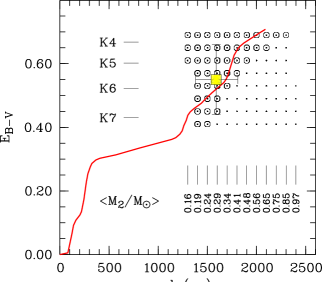
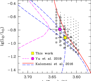
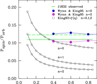
Figure 9: Left: Confidence range for models of the secondary star permitted by the photometric SED in the eclipse of J1832 (dots and encircled dots). All models have distances within the error bounds of Gaia EDR3 (footnote 3). The red curve represents the best estimate of the extinction along the line of sight to J1832 (Lallement et al., 2018). Center: Position of the secondary star of J1832 in its HR diagram. The dots indicate all photometrically accepted models. The encircled dots denote here and in the left panel the subsample with luminosity $L_{2}$ not exceeding the limit set by the BPS of Kalomeni et al. (2016) (red curve). No model should be found above and to the right of the red curve (see text). The yellow-filled square in both panels marks the mean position of this subsample. The dashed blue curves from Kalomeni et al. (2016) indicate two evolutionary tracks along which J1832 may evolve. Also shown are the position of the 9 h binary KIC 5608384 of Yu et al. (2019) (magenta dot) and its suggested evolutionary track that leads to the graveyard of ultracompact binaries (magenta dashed curve). Right: period ratio $P_{\mathrm{spin}}/P_{\mathrm{orb}}$ vs. mass ratio $q$. The horizontal green lines indicate the observed period ratio of J1832. The open and filled circles denote the theoretical period ratios from the analytical theory of K93 and the numerical calculations of WK95.

In the absence of spectroscopy, the information on the system parameters is limited. Some important information, however, can be drawn from the measured $i$-band magnitude of the secondary star. In particular, it allows $M_{2}$ to be calculated as a function of the distance, $d$, with a minor dependence on $E_{\mathrm{B-V}}$. The quantities are related by the surface brightness $S_{\mathrm{i}}\!=\!M_{\mathrm{i}}\,+\,5\,\mathrm{lg}(R_{2}/R_{\odot})$, where $M_{\mathrm{i}}$ is the absolute magnitude in the $i$-band and $R_{2}$ the stellar radius. Using Mamajek’s table of the stellar locus (footnote 5) with colors transformed to the Pan-STARRS 1 (P1) system, we expressed the surface brightness for the restricted range of $(r\!-\!i)_{\mathrm{P1}}$ = 0.3 - 0.8 as

$$S_{\mathrm{i}}=5.151-1.867\,(r-i)_{\mathrm{P1}}.$$ (8)

With $i-M_{\mathrm{i}}\,=\!5\,\mathrm{lg}\,d\!-\!5$ and $d$ in pc, $R_{2}$ in solar units becomes

$$\mathrm{lg}(R_{2}/R_{\odot})\,=\!(S_{\mathrm{i}}-i+A_{\mathrm{i}}E_{\mathrm{B-V}})/5+\mathrm{lg}\,d-1.$$ (9)

Since J1832 is accreting, the secondary star must fill its Roche lobe and is necessarily bloated if of low mass. We adopted the model radii of Baraffe et al. (2015) for main-sequence stars of solar composition at an age of 5 Gyr and approximated them by a power law $R_{\mathrm{BHAC}}/R_{\odot}=a(M_{2}/M_{\odot})^{b}$ with $a=0.93$ and $b=0.96$ for the mass range of $0.15-0.8$ $M_{\odot}$. Secondary stars in normal CVs are known to exceed these radii by a few percent (Knigge et al., 2011, see also Beuermann et al. 2017). We expressed the stellar radii in our models as $R_{2}\!=\!f_{1}f_{2}f_{3}R_{\mathrm{BHAC}}$, with $f_{1}\!=\!1.020$ and $f2\!=\!1.045$ accounting for starspots and the effect of rotation and Roche geometry, respectively (Knigge et al., 2011). The factor $f_{3}$ describes any additional bloating required to make the secondary star fill its lobe. We used Paczynski’s approximation $R_{\mathrm{2,R}}\,=\!0.462(q/(1+q)^{1/3}a$ for the mean volume filling Roche radius, which has the advantage that with the binary separation $a$ eliminated with help of Kepler’s third law, one obtains an expression that is independent of $q$ and $M_{1}$

$$M_{2}/M_{\odot}\,=\!(R_{2}/R_{\odot})^{3}(2\pi/P)^{2}(R_{\odot}^{3}/(0.462^{3}\mathrm{G}M_{\odot})).$$ (10)

Replacing $R_{2}/R_{\odot}$ with Eqs. 9, 8, and 7, $M_{2}$ can be calculated for given $d$ and $E_{\mathrm{B-V}}$. For instance, for a distance of 1600 pc and the best-fitting extinction of 0.54 mag, $M_{2}\!=\!0.29$ $M_{\odot}$. To fill its Roche-lobe, this star would be bloated by a factor $f_{3}\!=\!2.27$ over its main-sequence radius. An unevolved secondary star of 1.0 $M_{\odot}$ as expected for a standard CV at $P\!\simeq\!9$ hr would require a distance of 2500 pc, near the upper end of the confidence range of the Gaia EDR3, $d\!=\!1254-2847$ pc (Bailer-Jones et al., 2021).

Table 5: Mean values and ranges of parameters of all photometrically accepted models (Cols. 3-5) and those in spin equilibrium with $P_{\mathrm{spin}}$$\,=\!3484$ s (Cols. 6-8; see text for explanation).

#   Quantity	Photometrically accepted					$L_{2}$-limited
	Mean	Sigma	Range			Mean	Sigma
1   $d$ (pc)	1755	284	1270	$-$	2500	1596	208
2   $E_{\mathrm{B-V}}$ (mag)	0.54	0.10	0.38	$-$	0.70	0.58	0.09
3   $(r\!-\!i)_{\mathrm{P1}}$ (mag)	0.48	0.07	0.36	$-$	0.60	0.45	0.07
4   $M_{2}$ ($M_{\odot}$)	0.41	0.20	0.16	$-$	1.00	0.32	0.14
5   $R_{2}=R_{\mathrm{Roche}}$ ($R_{\odot}$)	0.73	0.12	0.54	$-$	1.00	0.67	0.09
6   $f_{3}$	2.03	0.61	1.02	$-$	3.31	2.33	0.56
7   $T_{\mathrm{eff,2}}$ (K)	4119	143	3918	$-$	4402	4185	136
8   $-$log($L_{2}/$$L_{\odot}$)	0.88	0.15	1.20	$-$	0.47	0.92	0.15
9   $M_{1}$ ($M_{\odot}$)	0.92	0.25	0.40	$-$	1.30	0.88	0.26
10   $q=M_{2}/M_{1}$	0.46	0.20	0.12	$-$	0.85	0.38	0.18
11   $i$ (°)	77.3	2.9	72.9	$-$	85.7	78.4	2.9
12   $a$ ($10^{11}$ cm)	1.64	0.16	1.24	$-$	1.99	1.59	0.15
13   $r_{\mathrm{ci}}$/$a$	0.13	0.03	0.10	$-$	0.21	0.14	0.03
14   $r_{\mathrm{co}}$/$a$ ($P_{\mathrm{spin}}$$\!=\!3484$ s)	0.20	0.01	0.19	$-$	0.22	0.21	0.01
15   $r_{\mathrm{co}}$/$a$ ($P_{\mathrm{spin}}$$\!=\!3911$ s)	0.22	0.01	0.20	$-$	0.24	0.22	0.01
16   $r_{\mathrm{ci}}$/$r_{\mathrm{co}}$ ($P_{\mathrm{spin}}$$\!=\!3484$ s)	0.65	0.09	0.54	$-$	0.94	0.68	0.09
17   $r_{\mathrm{ci}}$/$r_{\mathrm{co}}$ ($P_{\mathrm{spin}}$$\!=\!3911$ s)	0.60	0.09	0.50	$-$	0.87	0.63	0.09
18   $L_{\mathrm{acc}}$ ($L_{\odot}$)(1)	2.10	0.79	0.89	$-$	5.53	1.95	0.75
19   $\dot{M}$ ($10^{-10}$$M_{\odot}$/yr)(1)	6.8	4.5	1.2	$-$	36.9	7.0	5.0
20   $T_{\mathrm{wd}}$ (kK) (2)	27.5	5.1	14.0	$-$	41.3	26.3	5.0
21   $R_{\mathrm{wd}}$ ($10^{8}$ cm)(3)	6.55	2.21	3.69	$-$	11.86	6.93	2.23
22   $r_{\mathrm{wd}}$ (mag)(4)	23.8	0.6	22.5	$-$	25.2	23.7	0.6
23   $g_{\mathrm{wd}}$ (mag)(4)	23.9	0.6	22.6	$-$	25.4	23.8	0.6
24   $\mu_{34}$ ($10^{34}$ G cm)	1.61	0.29	0.90	$-$	2.43	1.57	0.31
25   $B_{\mathrm{surf}}$ (MG)(5)	100	82	7	$-$	348	85	76
26   $K_{1}$ (km s-1)	96	32	37	$-$	169	81	27
27   $K_{2}$ (km s-1)	219	34	139	$-$	299	225	37

(1) Based on case-B accretion-induced flux; (2) Based on $\dot{M}$ in line 19 and Eq. 11; (3) Based on $M_{1}$, $T_{\mathrm{wd}}$, and WD models with a thick hydrogen envelope (Althaus & Benvenuto, 1998; Renedo et al., 2010); (4) Reddened model magnitudes; (5) Based on lines 21 and 24.

5.2 Grid of photometrically accepted models

We computed a grid of dynamical models of J1832 that extended over $d\!=\!1200-2900$ pc and $E_{\mathrm{B-V}}$$=0.37-0.71$ with step widths of 10 pc and 0.01, respectively. Each bin is characterized by the single value of $M_{2}$($d$,$E_{\mathrm{B-V}}$) that matches the observed $i\!=\!18.98$ (Table 4) and contains models for $M_{1}$ between 0.40 and 1.30 $M_{\odot}$ with a step width of 0.01 $M_{\odot}$. As side conditions we required $q\!<\!0.85$, which ensures stable mass transfer, and $M_{2}\!>\!0.16$ $M_{\odot}$, which accounts for the strict lower limit to $M_{2}$ in evolving CVs with 9 hr orbital period in the binary population study (BPS) of Kalomeni et al. (2016), as defined by their Eq. 12. For each individual model, we calculated a wide range of system parameters. Results are provided in columns $3\!-\!5$ of Table 5. A coarser version of the grid with steps of 0.04 in $E_{\mathrm{B-V}}$ and 100 pc in $d$ was used for Fig. 9. The left panel shows all photometrically accepted models in the $d$-$E_{\mathrm{B-V}}$ plane as dots or circled dots. They cover a distance range that stays well within the Gaia EDR3 confidence limits (Bailer-Jones et al., 2021): There are no accepted models at $d\!<\!1270$ pc, because $M_{2}$ would fall below $0.16$ $M_{\odot}$, and none at $d\!>\!2500$ pc, because $q\!>\!0.85$ or $M_{1}\,>\!1.3$ $M_{\odot}$ would be required. The $M_{2}$ values quoted in the figure are the averages of $M_{2}(d,E_{\mathrm{B-V}})$ over $E_{\mathrm{B-V}}$ for the selected distance. The quoted spectral types are obtained from $E_{\mathrm{B-V}}$ via $(r\!-\!i)_{\mathrm{P1}}$ and do not depend explicitly on $d$. The center panel shows the accepted models in the $T_{\mathrm{eff,2}}$$-$log($L_{2}/L_{\odot}$) plane, the Hertzsprung-Russell (HR) diagram of the secondary star. The right panel shows the theoretical results on the $q$ dependence of the period ratio $P_{\mathrm{spin}}/P_{\mathrm{orb}}$ together with the observed level in J1832(green lines). These results are now discussed in turn.

5.3 J1832 in the Hertzsprung-Russell diagram

Using the stellar-locus tables of Mamajek (Pecaut & Mamajek, 2013, see footnote 5) and Mann et al. (2015), we constructed the color dependence of the effective temperature $T_{\mathrm{eff,2}}$ of the secondary star as a function of $(r\!-\!i)_{\mathrm{P1}}$. Each of our models is tagged by a value of $(r\!-\!i)_{\mathrm{P1}}$ and a value of $T_{\mathrm{eff,2}}$. Combined with $R_{2}$ from Eq. 9, we calculated log($L_{2}/L_{\odot}$) for all models and thereby their position in the HR diagram of the secondary star. The center and left panels of Fig. 9 show the same photometrically accepted models as small black dots. The center panel includes, in addition, results of the BPS of Kalomeni et al. (2016). The red curve indicates the strict upper limit to the luminosity $L_{2}$ of the secondary star as a function of $T_{\mathrm{eff,2}}$, taken from their Fig. 20. Our photometrically accepted models are distributed across this line and for about 50% of them the secondary star is too bright by up to a factor of 2.6. The encircled dots indicate the luminosity-restricted sample of models that are consistent with the Kalomeni et al. (2016) BPS calculations, allowing for a 10% uncertainty and spillover in $L_{2}$. We list the mean values and standard deviations of all parameters of the luminosity-restricted sample in columns 6 and 7 of Table 5. The centroid of this restricted sample is indicated by the yellow squares and given by $d\!=\!1596\!\pm\!208$ pc, $E_{\mathrm{B-V}}$$\,=\!0.58\!\pm\!0.09$, $M_{2}\!=\!0.32\!\pm\!0.14$ $M_{\odot}$, $T_{\mathrm{eff,2}}$$\,=\!4185\!\pm\!136$ K, and log($L_{2}/L_{\odot}$)$\,=\!-0.92\!\pm\!0.15$, where the quoted errors represent the standard deviations of the distributions and we consider all models a priori as equally probable. The strongly skewed $M_{2}$ distribution of the luminosity-restricted sample still contains $M_{2}$ values up to 1.0 $M_{\odot}$, but all models with secondary masses $M_{2}$ more than 2 $\sigma$ above the mean, or $M_{2}\!>\!0.60$ $M_{\odot}$, lie in the extended tail of the distribution at $d\!>\!1980$ pc in the left panel and at log($L_{2}/L_{\odot}$)$\,>\!-0.68$ in the center panel of Fig. 9. This tail contains 5% of the models. We consider them correspondingly unlikely and take this as an indication of a low-mass secondary star in J1832, with $M_{2}$ lower than expected for a normal CV of 9 hr orbital period.

The two dashed blue curves in the center panel of Fig. 9 show two selected evolutionary tracks of CVs from the BPS calculations of Kalomeni et al. (2016, their Figs. 20 and 1), a normal one with a secondary near the main sequence that evolves close to the red line and a binary with an evolved secondary of lower mass that departs from that track and heads for the lower left of the diagram into the general region occupied by ultracompact binaries. They represent possible evolutionary scenarios for J1832. In the former case, J1832 would probably evolve into a polar, and in the latter, it might follow the 9 h binary KIC 5608384 of Yu et al. (2019) (magenta dot and magenta dashed curve) to become an ultracompact binary, with the decisive difference of one component being highly magnetic.

5.4 Accretion rate and WD temperature

We have no good handle yet on the accretion rate of J1832, but it is useful to obtain at least an estimate. Assuming isotropic emission, the accretion luminosity is $L_{\mathrm{acc}}\!\simeq\!4\pi d^{2}F_{\mathrm{acc}}$ and the accretion rate is estimated as $\dot{M}\!\simeq\!L_{\mathrm{acc}}R_{1}/\mathrm{G}M_{1}$. So far, only the optical part $F_{\mathrm{opt}}$ of the accretion-induced high-state flux $F_{\mathrm{acc}}$, is available. We identify it with the upper envelope to the observed (reddened) fluxes in the left panel of Fig. 8. Integrated from the Balmer edge into the infrared they give $F_{\mathrm{opt,red}}\!=\!2.5\,\times\!10^{-12}$ erg cm^-2s^-1. For each model, we obtained the individually de-reddened value of $F_{\mathrm{opt}}$ and estimated $F_{\mathrm{acc}}\!=\!(1+f_{\mathrm{uvx}})\,F_{\mathrm{opt}}$ with a correction factor $f_{\mathrm{uvx}}$ that accounts for the still missing UV and X-ray fluxes. We considered two cases, of which case A with $f_{\mathrm{uvx}}\!=\!0$ or $F_{\mathrm{acc}}\!\equiv\!F_{\mathrm{opt}}$ represents the absolute minimum. Guided by the well-studied IPs EX Hya and V1223 Sgr (Eisenbart et al., 2002; Beuermann et al., 2004), we adopted case B with $f_{\mathrm{uvx}}\!=\!2.0$ or $F_{\mathrm{acc}}\!=\!3.0\times F_{\mathrm{opt}}$, accounting for an ultraviolet flux as in other IPs and a moderate X-ray flux. In what follows we use case B in the attempt to obtain an overview of the system parameters. The range of case-B accretion rates is listed in line 19 of Table 5.

The secular mean accretion rate $\langle\dot{M}\rangle_{\mathrm{10}}$ of systems with a sufficiently old WD averaged over its Kelvin-Helmholtz timescale determines its effective temperature by compressional heating,

$$T_{\mathrm{eq}}\!=\!18.9\,\langle\dot{M}\rangle_{\mathrm{10}}^{1/4}\,M_{1}\leavevmode\nobreak\ \leavevmode\nobreak\ \mathrm{kK}$$ (11)

(Townsley & Gänsicke, 2009), where $\langle\dot{M}\rangle_{\mathrm{10}}$ is in units of $10^{-10}$ $M_{\odot}$yr^-1 $M_{1}$ in solar units. We estimated the current WD temperature by replacing $\langle\dot{M}\rangle_{\mathrm{10}}$ in Eq. 11 with the case-B accretion rate for each model. The resulting mean temperature of all photometrically accepted models is 27 kK (line 15 of Table 5). The corresponding reddened WD AB magnitudes are $r\!=\!22.56-25.16$ and $g\!=\!22.57-25.39$, which are all at least 1 mag fainter than our observed 2$\sigma$ upper limits of 21.44 and 21.69, respectively (Sect. 4.2). The faintest WDs are found in the most distant models with a primary mass of 1.3 $M_{\odot}$.

5.5 Orbital inclination

We estimated the inclination of J1832, using the Roche lobe parameters $x_{1}\!=b/a$, $x_{4}$, $y_{4}$, $z_{6}$, and $r_{2}^{*}$ in the notation of Kopal (1959), expressed as functions of the mass ratio $q$. For a given duration of the eclipse in phase units, the orbital inclination is a function of $q$ (e.g., Horne, 1985). For J1832, the inclination is 87$\aas@@fstack{\circ}$6, 81$\aas@@fstack{\circ}$8, 77$\aas@@fstack{\circ}$4, or 73$\aas@@fstack{\circ}$3 for $q\!=\!0.1,0.2,0.4$, or 0.8, respectively. The path of the WD across the shadow of the secondary star defines an arced section with a chord length $\rho$ and a height $\sigma$, which are also functions of $q$. For the luminosity-selected sample in Fig. 9 (encircled dots), the mean inclination is 78$\aas@@fstack{\circ}$4 and the full range is $72\aas@@fstack{\circ}9\!-\!85\aas@@fstack{\circ}7$ (Table 5). At eclipse center, the WD has dived into the shadow of the secondary star to a mean depth $\sigma\,=\!20.6$$R_{\mathrm{wd}}$ (full range $6.2\!-\!58.2$$R_{\mathrm{wd}}$). The magnetically guided part of the accretion stream reaches a similar height above the orbital plane and, depending on the details of the accretion geometry, only a small part of the stream emission escapes eclipse. Hence, the system qualifies as deeply eclipsing.

5.6 The magnetic moment of the WD

In an IP, matter accretes to the magnetic field of the WD near the magnetospheric radius, $r_{\mathrm{mag}}$, which is usually quoted as a fraction of the Alfvén radius, $r_{\mathrm{alf}}$. The latter is obtained by equating the ram pressure of the infalling matter for isotropic accretion with the magnetic pressure of a dipolar field. The rapid drop of the magnetic pressure with increasing radius as $r^{-6}$ implies that the usual estimate of $r_{\mathrm{mag}}$$\,\simeq\!0.5\,$$r_{\mathrm{alf}}$ cannot be severely wrong. The factor 0.5 accounts for the difference between spherical and equatorial accretion (Frank et al., 2002), and results in

$$r_{\mathrm{mag}}\,\simeq\,2.2\,\times\!10^{8}\dot{M}_{10}^{-2/7}M_{\mathrm{wd}}^{-1/7}\mu_{30}^{4/7}\leavevmode\nobreak\ \leavevmode\nobreak\ \leavevmode\nobreak\ \mathrm{cm}.$$ (12)

For each of our models of J1832, we obtained an estimate of the magnetic moment $\mu_{30}$ of the WD in units of $10^{30}$ G cm³ by using the case-B accretion rate in units of $10^{-10}$ $M_{\odot}$yr^-1, the WD mass in solar units, and equating $r_{\mathrm{mag}}$ with the corotation radius $r_{\mathrm{co}}$$\,=\!(GM_{1}/\omega_{\mathrm{s}}^{2})^{1/3}$. For the sample of models restricted by the photometry and luminosity of the secondary star (encircled dots in Fig. 9), we found a mean magnetic moment $\mu\!=\!(1.6\,\pm\,0.3)\,\times\!10^{34}$ G cm³ (Table 5, line 24), which is at the upper limit of the range discussed for IPs (Norton et al., 2004) and is more characteristic of a polar. The implied field strength would be typical of or exceed that of a polar as well.

5.7 Spin equilibrium

Most IPs are expected to accrete in spin equilibrium ($\dot{P}_{\mathrm{spin}}=0$), because a mismatch between the velocities of matter and field at the accretion radius $r_{\mathrm{acc}}$ leads to rapid spin-up or spin-down of the WD, ensuring $r_{\mathrm{mag}}$$\,\simeq\,$$r_{\mathrm{acc}}$$\,\simeq\,$$r_{\mathrm{co}}$ most of the time. Matter leaving $L_{1}$ with a specific angular momentum $j_{\mathrm{L1}}\!=\!b^{2}\Omega_{\mathrm{o}}$ will settle into a Keplerian orbit at the circularization radius $r_{\mathrm{ci}}$ with $j_{\mathrm{ci}}\!=\!(\mathrm{G}M_{1}r_{\mathrm{ci}})^{1/2}\!=\!j_{\mathrm{L1}}\zeta$, giving $r_{\mathrm{ci}}$$\,=\!(1\!+\!q)(b/a)^{4}\zeta^{2}$. Here, $b$ is the separation between the WD and $L_{1}$, $\Omega_{\mathrm{o}}\!=\![GM_{1}(1\!+\!q)/a^{3}]^{1/2}$ is the orbital frequency, and $\zeta(q)\!\simeq\!0.84\!-\!0.89$ for $q\!=\!1.0\!-\!0.1$, respectively, is the fraction of the angular momentum at $L_{1}$ that is preserved at $r_{\mathrm{ci}}$, when the pull of the secondary star or the non-sphericity of the problem is accounted for (Flannery, 1975; Lubow & Shu, 1975). For $r_{\mathrm{mag}}$$\,\simeq\,$$r_{\mathrm{co}}$$\,\ga\,$$r_{\mathrm{ci}}$, a viscous disk cannot form and the WD accretes from the stream, either directly or after circularization. This is obviously the case in J1832: the entire sample of our dynamical models that match the photometry of J1832 (dots and circled dots in Fig. 9) have $r_{\mathrm{co}}$$\,>\,$$r_{\mathrm{ci}}$ (Table 5, lines 13 to 17).

King & Lasota (1991) argued that the accretion of $j_{\mathrm{ci}}\!=\!j_{\mathrm{L1}}\zeta$ in spin equilibrium implies $r_{\mathrm{co}}$$\,\simeq\,$$r_{\mathrm{ci}}$ as well, leading to

$$P_{\mathrm{spin}}/P_{\mathrm{orb}}=\Omega_{\mathrm{o}}/\omega_{\mathrm{s}}\simeq(1+q)^{2}(b/a)^{6}\zeta^{3},$$ (13)

where $b/a\!\simeq\!0.500\!-\!0.227$log $q$ (Plavec & Kratochvil, 1964). They identified the preferred occurrence of IPs near $P_{\mathrm{spin}}/P_{\mathrm{orb}}$$\,=\!0.10$ with stream-fed accretion in spin equilibrium. A period ratio of 0.10, however, or larger as in J1832, requires $q\!\la\!0.15$, which is much lower than the typical $q\!\approx\!0.6$ for nine IPs above the period gap that have measured component masses (Ritter & Kolb, 2003). The likely cause is that $r_{\mathrm{co}}$ and $r_{\mathrm{ci}}$ do not agree as closely as assumed. As a consequence, a reliable value of $q$ for J1832 cannot be obtained from Eq. 13.

The relation between $r_{\mathrm{co}}$ and $r_{\mathrm{ci}}$ in spin equilibrium is determined by the exchange of angular momentum between matter and field inside and outside $r_{\mathrm{co}}$, which may take place over a substantial radial interval. An example is the accretion from a viscous disk. Another is the accretion of a stream of diamagnetic blobs of matter studied analytically by King (1993) (henceforth K93) and numerically by Wynn & King (1995) (henceforth WK95). Such blobs plunge deep into the magnetosphere on quasi-ballistic orbits, experience a drag by the excitation of Alfvén waves, when they move across field lines and “pluck them like violin strings” (Drell et al., 1965), until they are broken up by Kelvin-Helmholtz instabilities, invaded by the field, and accreted (Arons & Lea, 1980). K93 made the problem analytically tractable by treating the blobs as test particles, disregarding changes in their internal state, neglecting viscous collisions between them, assuming spherical symmetry ($\zeta\!=\!1$), selecting a simple parameterization of the drag, and describing the blob orbits as Kepler ellipses that slowly change under the influence of the drag. He described the drag as $\@vec{F}\!=\!-k_{0}\,r^{-n}\@vec{\upsilon}$, where, $\@vec{\upsilon}$ is the velocity of the blob relative to the field and the integer $n\!\geq\!0$ regulates the radial dependence of the drag. The azimuthal motion of a blob is typically accelerated near apastron and decelerated near periastron, which circularizes the orbit. K93 expressed the equilibrium period ultimately as a function of $n$ and $q$ (his Eqs. 38 ff). The relation between the characteristic radii becomes $r_{\mathrm{ci}}$$\,=\!(f/g)^{2/3}\,$$r_{\mathrm{co}}$, with functions $f(q)$ and $g(q)$ for a given parameter $n$. This relation bears a formal similarity to $r_{\mathrm{in}}\!=\!\omega_{\mathrm{s}}^{2/3}r_{\mathrm{co}}$ for disked systems (Wang, 1995), with $\omega_{\mathrm{s}}$ the fastness parameter (not to be mixed up with the spin angular velocity). In both cases a competition exists between orbits that accelerate the magnetosphere inside $r_{\mathrm{co}}$ and decelerate it outside $r_{\mathrm{co}}$. The decisive dissimilarity is the absence of viscous inter-blob interactions in the model of K93 and WK95, which holds as long as the blobs do not accumulate and form a nascent disk. Consequently, the radial transport of angular momentum, characteristic of an accretion disk, is absent in the model of K93 and leads to a relation between $P_{\mathrm{spin}}/P_{\mathrm{orb}}$ and $q$ (his Eq. 37),

$$P_{\mathrm{spin}}/P_{\mathrm{orb}}=(1+q)^{2}\leavevmode\nobreak\ (b/a)^{6}\,(g/f)\leavevmode\nobreak\ \zeta^{3},$$ (14)

where we have added the factor $\zeta^{3}$ to correct approximately for the neglect of the gravitational pull of the secondary star. The functions $f(q)$ and $g(q)$ are given by K93 and WK95 for $n\!=\!0,2$, and 3. For $n\!=\!1$, $g/f\!=\!1$. The numerical study of WK95, treating the particle orbits correctly in the nonspherical geometry, gave period ratios that consistently exceeded the analytical results, less so for $n\!=\!0$ than for positive $n$. Unfortunately, only two sets of results for $P_{\mathrm{spin}}/P_{\mathrm{orb}}$ versus $q$ were published.

In the right panel of Fig. 9, we compare the $q$ dependence of $P_{\mathrm{spin}}/P_{\mathrm{orb}}$ obtained from the analytical and numerical calculations of K93 and WK95 for $n\!=\!0$ to 2 with the level of the observed $P_{\mathrm{spin}}/P_{\mathrm{orb}}$ of J1832 (green lines). As noted in Eq. 14, the correction $\zeta(q)$ from Lubow & Shu (1975) has been applied to the analytical period ratios, while the numerical ones correctly account for the non-sphericity of the gravitational field. We note that the numerical values of $\zeta$ displayed in Fig. 1 of King et al. (1990) show the opposite trend from those of Lubow & Shu (1975), which leads to a period ratio in WK95 that varies little with $q$. The numerical results exceed the analytical ones by about 30% for $n\!=\!0$ and by more for $n\!=\!2$. The analytical $n\!=\!0$ model and the numerical $n\!=\!0$ and $n\!=\!2$ models best match the observed period ratio of J1832. Hence, the K93 and WK95 models support the nature of J1832 as a stream-fed IP in spin equilibrium, but they are not sufficiently accurate to allow a determination of $q$ from $P_{\mathrm{spin}}/P_{\mathrm{orb}}$.

6 Discussion

J1832.4-1627 is the first deeply eclipsing stream-fed IP. It is disk-less in the sense that it lacks a viscous (i.e., luminous) accretion disk. It combines two properties that are extremely rare within the class. There are only five IPs that display deep eclipses of the central accretion region surrounding the WD, the two long-known systems DQ Her and XY Ari, V902 Mon=IPHAS J0627 (Aungwerojwit et al., 2012), Nova Sco 1437 (Potter & Buckley, 2018, and references therein), and V597 Pup, the now faint remnant of Nova Puppis 2007 Warner & Woudt (2009), and all of them accrete via disks. Stream-fed systems are even less common and none of the candidates is eclipsing. The identification of a stream-fed system may be ambiguous because of the phenomenon of stream overflow that occurs also in disked systems (Lubow, 1989). The best and so far only example of a stream-fed IP is V2400 Oph (Buckley et al., 1995, 1997; Hellier & Beardmore, 2002; Joshi et al., 2019), which, however, is seen at an inclination of only $i\!\sim\!10$°, preventing a measurement of its component masses. The combination of a deep eclipse and a stream-fed and seemingly disk-less accretion geometry in J1832 is unique with important prospects for follow-up studies.

Our Fourier and periodogram analyses gave a clear signal at a single period $P_{\mathrm{obs}}$$\,=\!3911$ s. Our data contain no hint for identifying it with either the spin or the synodic period. If a stream of tenuous matter impinges on the magnetosphere, is instantaneously permeated by the field, and accreted on the spot, the resulting signal will be pulsed at the synodic (beat) period. Such matter is generally hold responsible for the emission of hard X-rays. Denser blobs of matter, on the other hand, continue on ballistic orbits in the magnetosphere and are carried around by the field until threaded. They lose the memory of the orbital phase of impact and the resulting emission is likely pulsed on the spin period. For a structured stream, covering a wide range of densities, a mixture of spin and synodic periods and their side bands may be expected (Warner, 1986), and a prediction for an individual wavelength band is not easily made. In the stream-fed IP V2400 Oph, the X-ray flux is pulsed at the synodic and the spin period (Buckley et al., 1997; Joshi et al., 2019), the optical circularly polarized flux appears at the spin period (Buckley et al., 1995), and the optical continuum preferentially at the synodic period (Hellier & Beardmore, 2002). Performing a hard X-ray study and optical circular spectropolarimetry are, therefore, the most obvious next steps for further study of J1832.

There is preliminary, and certainly incomplete, evidence that J1832 may not be a strong X-ray source (Sect. 4.3). With an interstellar atomic hydrogen column density $N_{\mathrm{H}}$$\,\simeq\!5\,\times\!10^{21}$ H-atoms cm^-2, based on $E_{\mathrm{B-V}}$$\,\simeq\!0.54$ (Nguyen et al., 2018), X-rays with $E\!<\!1$ keV would be absorbed. A strong soft X-ray component was observed in some IPs (e.g., PQ Gem, V405 Aur, and UU Col), and such a source would not be detectable in J1832. The spectroscopic detection of He ii$\lambda$4686 line emission would, however, demonstrate the presence of such a source. Other IPs emit hard X-rays, possibly reflecting differences in the accretion geometry and in the density structure of the accreted matter. For example, Nova Sco 1437 and XY Ari are strong hard X-ray sources, while IPHAS J0627 is faint. Aungwerojwit et al. (2012) argued that the X-ray emission region in IPHAS J0627 may be obscured by the inner edge of the disk, but this may not be the whole story.

The lack of a luminous disk and the observed stream flipping in J1832 are not short-lived transitory phenomena. The evidence for the stream flipping is based on the pulse phase dependence of the eclipse centers and the orbital phase dependence of the pulse minima observed in all three observing seasons (Sect. 3.4). These results strongly suggest that J1832 is stream-fed, a conclusion that is supported also by the fact that all of our photometrically accepted models have $r_{\mathrm{co}}$$\,>\,$$r_{\mathrm{ci}}$ and, hence, lack a classical viscous disk. The accretion process is regulated by the hierarchy between three characteristic timescales, the dynamical (Kepler) timescale $t_{\mathrm{kep}}$, the threading timescale $t_{\mathrm{mag}}$, and the viscous timescale $t_{\mathrm{vis}}$. On-the-spot accretion takes place for $t_{\mathrm{mag}}$$\,\ll\,$$t_{\mathrm{kep}}$, while the matter is circularized before being accreted for $t_{\mathrm{mag}}$$\,\gg\,$$t_{\mathrm{kep}}$, assuming in both cases that $t_{\mathrm{vis}}$ is much longer. A theory for the former case that allows for a structured stream is not available. A theory for the latter, assuming the accretion of dense diamagnetic blobs of matter, was devised by K93 and WK95 and discussed in Sect. 5.7. In their model, the matter is circularized by the drag it experiences when crossing field lines. It does not spread into a disk as long as $t_{\mathrm{mag}}$ stays sufficiently short and the blobs do not accumulate and get viscously into contact. Because of the similarities with disk theory, K93 insisted on calling his accretion mode stream-fed and not disk-less. A relation of the form of Eq. 14 exists for stream-fed, but not for disk-fed systems. It is, however, burdened by the factor $g/f$ in the theory of K93 or a corresponding factor in any alternative theory.

The factual absence of viscous interaction would render any ring-like structure cool. On the other hand, if it is irradiated and heated by a central X-ray source, it may be difficult to hide it at optical wavelengths. In any case, the presence of Balmer and helium line emission may help to trace the geometry of the magnetically guided stream and the potential presence of an accretion ring. K93 estimated that individual blobs may survive in the vicinity of $r_{\mathrm{co}}$ for up to ten orbits around the WD, before they lose their identity, are invaded by the field, and accreted. We estimated the times scales $t_{\mathrm{drag}}$ of Drell et al. (1965) and K93 and $t_{\mathrm{evap}}$ of Arons & Lea (1980) for the parameters of J1832 and obtained smaller numbers comparable to one pulse period of the WD, which is not enough to establish a ring, but sufficient for the matter to lose the memory of the impact point. Whether a well developed ring exists in J1832 and whether the synodic or spin period is preferred for the optical continuum emission are, therefore, open questions.

Of the stellar components, we have a secure photometric detection of the secondary star at the center of the eclipse, with a Pan-STARRS i-band AB magnitude of 18.98(3) and a spectral type $\sim\,$K6. The mean $M_{2}$ of the models that fit the photometry (Table 5, column 7) is $0.32$ $M_{\odot}$ and the 2$\sigma$ range is $0.16\!-\!0.60$ $M_{\odot}$. The secondary star is bloated over a main sequence star by a factor $f_{3}\!=\!1.4\!-\!3.3$ (Table 5). This finding suggests that J1832 may have previously passed through a phase of thermal timescale mass transfer, which would determine its future evolution as well. From its present position in the HR diagram of the secondary star (Fig. 9, center panel), the system may either still evolve into a polar or end up as an ultracompact binary, as predicted also for the nonmagnetic CV KIC 5608384 (Yu et al., 2019), but in the present case one of the final degenerate components would be strongly magnetic.

Detecting the WD in J1832 will not be a trivial task, given the 2$\sigma$ upper limits to its reddened (observed) magnitude of $g\!>\!21.69$ and $r\!>\!21.44$ (Sect. 4.2). Our dynamical models suggest probable magnitude ranges of $g\!=\!23.8\!\pm\!0.6$ and $r\!=\!23.7\!\pm\!0.6$, but the WD may reach 25 mag in both colors if the WD mass is as high as 1.3  $M_{\odot}$. The quoted magnitudes are based on the radii of WDs with a thick hydrogen envelope (Althaus & Benvenuto, 1998; Renedo et al., 2010) and effective temperatures computed from Eq. 11 with the long-term accretion rate replaced by the current case-B rate (Sect. 5.4). They disregard accretion-heated hot polar caps and can only be approximate. The dK6 secondary star with $r\!=\!18.98$ can be traced spectroscopically by its photospheric absorption lines or by emission lines from its face heated by the WD. Given the frequent low states, a phase-resolved study appears feasible. Tracing the motion of the WD will be more challenging. The predicted velocity amplitudes $K_{1}$ and $K_{2}$ of primary and secondary star are quoted in Table 5.

The estimated magnetic moment of the WD in J1832 of $\mu\!\simeq\!1.6\,\times\!10^{34}$ G cm³ suggests a surface field strength typical of polars (Norton et al., 2004). Hence, studying the magnetic field structure by means of spectropolarimetry and cyclotron spectroscopy seems a realistic prospect. Besides the high magnetic moment, the comparatively low accretion rate in the high state, assuming case-B to be valid, is reminiscent of long-period polars (Townsley & Gänsicke, 2009). While low in comparison with nonmagnetic CVs, the case-B accretion rate substantially exceeds that expected from gravitational radiation.

7 Outlook

We have presented a detailed photometric study of the first deeply eclipsing stream-fed IP that demonstrably lacks a viscous accretion disk. The $grizy$ photometry through the total eclipse yielded the magnitude and spectral type of the moderately evolved secondary star, while the WD has so far remained undetected. The Milky Way object is tolerably absorbed at a distance of about 1.6 kpc and is observable from both hemispheres. Key follow-up observations include: (i) a hard X-ray study and optical circular polarimetry to identify the spin period; (ii) phase-resolved optical spectroscopy to measure the velocity structure of the stream and the HeII$\lambda$4686 emission line flux; (iii) high-cadence high-state blue photometry through the eclipse to obtain information on the accretion geometry; (iv) the same in a deep low state to measure the diameter and mass of the WD; (v) high-resolution spectroscopy of the K star in a low state; and (vi) circular spectropolarimetry to measure the strength and structure of the magnetic field of the WD. A dedicated theoretical study is needed to understand its past and future evolution.