Magnetic Structures of Electron Systems on the Extended Spatially Completely
Anisotropic Triangular Lattice near Quantum Critical Points

Abstract

We examine magnetic structures of electron systems on an extended triangular lattice that consists of two types of bond triangles with electron transfer energies $t_{\ell}$ and $t_{\ell}^{\prime}$ ($\ell=1$, 2, and 3), respectively. We examine the ground state in the mean-field theory when $t_{1}=t_{1}^{\prime}$, focusing on collinear states with two sublattices. It is shown that when the imbalance of the spatial anisotropies of the two triangles is large, up-up-down-down (uudd) phases are stable, and the most likely ground states of the $\lambda$-${\rm(BETS)_{2}FeCl_{4}}$ system are the Néel state with the modulation vector $(\pi/c,\pi/a)$ and a uudd state, where $c=a_{1}=a_{1}^{\prime}$ and $a=(a_{2}+a_{2}^{\prime})/2$, with $a_{1}$, $a_{1}^{\prime}$, $a_{2}$, and $a_{2}^{\prime}$ being the lattice constants of the bonds with $t_{1}$, $t_{1}^{\prime}$, $t_{2}$, and $t_{2}^{\prime}$, respectively. These results are consistent with those from the classical spin system. In addition, this study reveals behaviors near the quantum critical point, which cannot be reproduced in the localized spin model. As the imbalance of the spatial anisotropies increases, the $U_{\rm c}$ of the Néel state increases, and that of the uudd state decreases. In the phase diagrams containing areas of the paramagnetic state, the Néel state with $(\pi/c,\pi/a)$, and a uudd state, their boundaries terminate at a triple point, near which all the transitions are of the first order. The phase boundary between the antiferromagnetic phases does not depend on $U$, and the transition is of the first order everywhere on the boundary. By contrast, the transitions from the two antiferromagnetic phases to the paramagnetic phase are of the second order, unless the system is close to the triple point.

1 Introduction

Electron systems on triangular lattices have been extensively studied because of intriguing phenomena, such as a possible quantum spin liquid, magnetic plateaus, spiral spin structures, and rich magnetic phase diagrams, [1, 2] all of which originate from frustration in spin alignment. The frustration is maximum when all the antiferromagnetic interactions on the bonds are equal; hence, spatial anisotropy, or inequality, of the interactions reduces the frustration. However, the influence of the spatial anisotropy can be practically significant when real compounds are examined. [3] For example, some organic compounds contain spatially anisotropic triangular lattices, shown in Fig. 1, that consist of two types of bond triangles; these lattices are called extended spatially completely anisotropic triangular lattices (ESCATLs). The model for localized spin systems has six types of exchange interactions with coupling constants $J_{\ell}$ and $J_{\ell}^{\prime}$, as shown in Fig. 1(a), while the model for itinerant electron systems has six types of transfer integrals $t_{\ell}$ and $t_{\ell}^{\prime}$, as shown in Fig. 1(b), where $\ell=1$, 2, and 3.

Interestingly, the ESCATL includes some frustrated lattices as special cases. It reduces to the spatially completely anisotropic triangular lattice (SCATL) when $J_{\ell}=J_{\ell}^{\prime}$ for all $\ell$, [3] and spatially anisotropic triangular lattice (SATL) when $J_{\ell}=J_{\ell}^{\prime}$ for all $\ell$ and $J_{2}=J_{3}$. [2] When $J_{3}^{\prime}=0$, the ESCATL reduces to the trellis lattice, [4] and when $J_{3}^{\prime}=J_{1}=J_{1}^{\prime}=0$, it reduces to the honeycomb lattice. [5] Compared with these reduced lattices, the ESCATL has a unique feature of an imbalance in the spatial anisotropies of the two bond triangles. [6]

In this study, we examine the itinerant electron systems on the ESCATL, being motivated by the organic compound $\lambda$-${\rm(BETS)_{2}}X{\rm Cl}_{4}$ (hereinafter abbreviated as $\lambda$-$X$), where $X={\rm Fe}$, ${\rm Ga}$, and ${\rm Fe}_{x}{\rm Ga}_{1-x}$. [7] These compounds have the ESCATL, as shown in Fig. 2, if each dimer of the BETS molecules is regarded as a site. The purposes of the study are to extend our knowledge on the ESCATL antiferromagnet and to gain theoretical insight into the magnetic structure in the $\lambda$-$X$ systems. In the $\lambda$-$X$ systems that exhibit an antiferromagnetic long-range order, it is considered that itinerant $\pi$-electrons principally sustain the order, and localized d-spins are passive in the exchange fields created by the $\pi$-electrons [8], which is the reason why we examine the itinerant electron model. We consider a realistic situation in which the spiral spin structure is suppressed; hence, we focus on collinear antiferromagnetic spin structures, such as the three Néel states defined in Fig. 3 and the two up-up-down-down (uudd) states defined in Fig. 4. We examine the ground state in the mean-field theory. To parameterize the imbalance of the spatial anisotropies mentioned above, we adopt

$$r_{\rm imb}\equiv\frac{t_{3}/t_{2}-t_{3}^{\prime}/t_{2}^{\prime}}{t_{3}/t_{2}}$$

because $t_{1}=t_{1}^{\prime}$ is satisfied in the $\lambda$-Fe system. [9]

(a)
(b)

Figure 1: Extended completely spatially anisotropic triangular lattice and definitions of (a) exchange coupling constants in localized spin systems and (b) transfer integrals in itinerant electron systems.

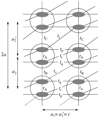
Figure 2: Schematic of the crystal structure of the BETS layers in the $\lambda$-$X$ system and the ESCATL. The small, dark ellipses and large circles represent BETS molecules and their dimers, respectively. The hopping integrals $t_{\rm A}$, $t_{\rm B}$, $t_{\rm C}$, $t_{\rm p}$, $t_{\rm q}$, $t_{\rm r}$, $t_{\rm s}$, and $t_{\rm t}$ are as defined by Kobayashi and Mori. [10] In terms of their hopping integrals, the hopping integrals in the present model are expressed as $t_{1}=t_{1}^{\prime}=(-t_{\rm p}-t_{\rm q}+t_{\rm r})/2$, $t_{2}=t_{\rm B}/2$, $t_{2}^{\prime}=t_{\rm C}/2$, $t_{3}=t_{\rm s}/2$, and $t_{3}^{\prime}=t_{\rm t}/2$. We refer to the lattice constants of the bonds with the hopping integrals $t_{1}$, $t_{1}^{\prime}$, $t_{2}$, and $t_{2}^{\prime}$ as $a_{1}$, $a_{1}^{\prime}$, $a_{2}$, and $a_{2}^{\prime}$, respectively, and define $c=a_{1}=a_{1}^{\prime}$ and $a=(a_{2}+a_{2}^{\prime})/2$. The lattice constant in the crystal a-axis of the compound corresponds to $2a$ in the present model.

Systems on the ESCATL are realized in other organic compounds such as $\lambda$-${\rm(BEST)_{2}}X{\rm Cl}_{4}$ and $\lambda$-${\rm(BEDT}$-${\rm STF)_{2}}X{\rm Cl}_{4}$ as well as the $\lambda$-$X$ systems, when each dimer of the molecules is regarded as a single lattice site. [11, 12, 9] In organic compounds of the form $D_{2}A$, where $D$ and $A$ represent a donor and an anion, respectively, the ESCATL can be realized when the donors are dimerized and the anions are in a staggered order. We examine wide parameter ranges, considering the potential for undiscovered compounds; however, we include candidate parameter sets for the $\lambda$-Fe system in the ranges so that the resulting phase diagrams include the points for this compound.

For the localized spin system on the ESCATL, classical phase diagrams [6] contain areas of the five collinear antiferromagnetic phases defined in Figs. 3 and 4 and the spiral spin phase. It was shown that the imbalance of the anisotropic parameters $J_{2}/J_{3}$ and $J_{2}^{\prime}/J_{3}^{\prime}$ stabilizes the uudd phases. Although similar uudd phases emerge in other systems, they are induced by four-spin, [13] ferromagnetic, [14, 15] and biquadratic exchange interactions. [16, 17] The present uudd phases are unique as they are induced solely by antiferromagnetic exchange interactions, where the other types of interactions are not required. Below, we clarify whether the uudd phases of this mechanism occur in itinerant electron systems as well as in the localized spin system.

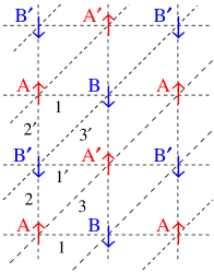
(a) Néel-$(\pi,\pi)$ state
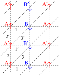
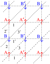
(b) Néel-$(\pi,0)$ state	(c) Néel-$(0,\pi)$ state

Figure 3: (Color online) Three Néel states and the definitions of the sublattices.

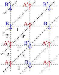
(a) uudd-2 state

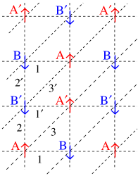
(b) uudd-$2^{\prime}$ state

Figure 4: (Color online) Two uudd states and the definitions of the sublattices.

Application to the $\lambda$-Fe system — In the next several paragraphs, we explain the background related to the $\lambda$-Fe system. The bonds along the crystal c- and a-axes of this system correspond to the $1$- and $1^{\prime}$-bonds and $2$- and $2^{\prime}$-bonds, respectively, as shown in Figs. 1–4. Although they are depicted as perpendicular for convenience, the c- and a-axes are not perpendicular in the $\lambda$-Fe system. The shear distortion gives rise to nonzero $t_{3}$ and $t_{3}^{\prime}$ in the present model.

In the classical spin model with parameter values for the $\lambda$-Fe system, [9] a spiral spin state has the lowest energy; [6] however, it would be reasonable to assume that this state is suppressed in this system because experimental studies suggest that the ground state is a collinear antiferromagnetic state. [18, 19, 20, 21, 22, 23, 24] In particular, an electron spin resonance (ESR) study suggests the existence of two sublattices in the magnetic field. [18] The possible reasons for the suppression of the spiral spin state are factors not incorporated in the classical spin model, such as quantum fluctuations and anisotropy in the exchange fields created by the d-spins. When the spiral spin state is excluded, the lowest-energy state is the Néel-$(\pi,\pi)$ state, and interestingly, the uudd-2 state has the second-lowest energy, which is slightly larger than the lowest energy. Because their difference is small and the estimated values of the energies contain errors due to simplifications in the model and errors in assumed parameters, it is reasonable to regard the Néel-$(\pi,\pi)$ and uudd-2 states as candidates for the ground state of the $\lambda$-Fe system.

Figure 5: Fermi surfaces for parameter sets ${\rm P}_{\rm K}$ (left panel) and ${\rm P}_{\rm M}$ (right panel) defined in Table 1.

Table 1: Values of transfer integrals in units of $10^{-2}$ eV. Parameter sets ${\rm P}_{\rm K}$ and ${\rm P}_{\rm M}$ are based on the values of transfer integrals obtained by Kobayashi and Mori, respectively. [10] The expressions for the transfer integrals $t_{\ell}$ and $t_{\ell}^{\prime}$ are given in the caption of Fig. 2. Parameter sets ${\rm P}_{\rm K}^{\prime}$ and ${\rm P}_{\rm M}^{\prime}$ are the variations of ${\rm P}_{\rm K}$ and ${\rm P}_{\rm M}$ in which $t_{3}$ is a variable and the other transfer integrals remain unchanged.

Transfer integral ${\rm P}_{\rm K}$ ${\rm P}_{\rm K}^{\prime}$ ${\rm P}_{\rm M}$ ${\rm P}_{\rm M}^{\prime}$ $t_{1}$  4.6325  4.6325  6.295  6.295 $t_{2}$  5.7555  5.7555  5.29  5.29 $t_{3}$  2.535 Variable  5.965 Variable $t_{2}^{\prime}$  4.145  4.145  6.205  6.205 $t_{3}^{\prime}$  0.1955  0.1955  0.965  0.965 $r_{\rm imb}$  0.891 $r_{\rm imb}(t_{3})$  0.862 $r_{\rm imb}(t_{3})$

The localized spin model can be an effective model for the $\lambda$-Fe system in the insulating phase; however, it misses the itinerant character of the $\pi$-electrons. In particular, they cannot take account of the fact that the $\lambda$-Fe system is possibly close to the quantum critical point ($U\approx U_{\rm c}$). [25, 26] Here, $U$ and $U_{\rm c}$ are the on-site Coulomb energy and the critical value of $U$ between the antiferromagnetic and paramagnetic states, respectively. Hence, the itinerant electron system is worth studying for the $\lambda$-Fe system.

The magnetic structure of the $\lambda$-Fe system was studied by some authors using models in which the $\pi$-electrons are itinerant. [27, 28, 29] Brossard et al. examined the magnetic structure of the d-spins in magnetic fields while treating the interaction between the d-spins in terms of the Ruderman-Kittel-Kasuya-Yosida (RKKY) interaction via conductive $\pi$-electrons. [27] Terao and Ohashi examined the superconductivity and antiferromagnetism by considering the RKKY interaction. [29] Hotta and Fukuyama examined the effect of d-spins on the $\pi$-electron system, considering the magnetic structure inside the dimers and obtained unified phase diagrams for some organic compounds [28]. These studies were based on a physical picture in which the antiferromagnetic transition is induced principally in the d-spin system because they were conducted before later experimental studies denied this picture. [30] This study is based on the current knowledge that the $\pi$-electron system is principal, whereas the d-spins are passive. Meanwhile, the magnetic structure inside the dimers [28] is beyond the scope of this study.

Because the $\lambda$-Fe system has Fermi surfaces open in the $k_{y}$-direction as shown in Fig. 5, it has often been suggested that the Fermi-surface nesting with the nesting vector near $(\pi/c,0)$ favors the antiferromagnetic order of this wave vector.[27, 9, 29] Here, it should be noted that the Fermi surfaces in Fig. 5 are drawn in the Brillouin zone halved by the difference between $(t_{2},t_{3})$ and $(t_{2}^{\prime},t_{3}^{\prime})$. The modulation vector $(\pi/c,0)$ in the half Brillouin zone cannot resolve the modulation vectors $(\pi/c,0)$ and $(\pi/c,\pi/a)$ in the original Brillouin zone, i.e., the Néel-$(\pi,0)$ and Néel-$(\pi,\pi)$ states defined in Figs. 3(a) and (b). Similarly, the modulation vector $(0,0)$ in the half Brillouin zone cannot resolve the modulation vectors $(0,0)$ and $(0,\pi/a)$ in the original Brillouin zone, i.e., the ferromagnetic state and the Néel-$(0,\pi)$ state defined in Fig. 3(c). The uudd phases have the modulation vector $(\pi/c,\pi/2a)$.

The experimental [22, 31, 32, 33] and theoretical [25] studies for the $\lambda$-${\rm Fe}_{x}{\rm Ga}_{1-x}$ system indicate that the influence of the d-spins is indispensable for the transition to the antiferromagnetic long-range order. This may appear inconsistent with the fact that the d-spins are passive; however, it can be explained on the basis of a stabilization effect [34, 35] by the anisotropy in the spin space and/or the enhanced three dimensionality introduced by the d-spins. These factors are not explicitly incorporated in the present model for the pure $\pi$-electron system; however, the stabilization of the long-range order by these factors is implicitly assumed in the present mean-field approximation.

In Sect. 2, we present the model and formulation. In Sect. 3, we present the numerical results including phase diagrams. Section 4 summarizes and discusses the results.

2 Model and Formulation

In the tight-binding model of the electron system on the ESCATL, electron energy dispersion can be written in the form [28]

$$\epsilon_{{{\bm{k}}}}=2t_{1}\cos k_{x}\pm\eta_{{{\bm{k}}}}$$ (1)

with

$$\begin{split}\eta_{{{\bm{k}}}}\equiv&\,\,\Bigl{\{}[(t_{2}+t_{2}^{\prime})\cos k_{y}+(t_{3}+t_{3}^{\prime})\cos(k_{x}+k_{y})]^{2}\\[-8.0pt] &~{}~{}~{}+[(t_{2}-t_{2}^{\prime})\sin k_{y}+(t_{3}-t_{3}^{\prime})\sin(k_{x}+k_{y})]^{2}\Bigr{\}}^{1/2}.\end{split}$$

The lattice constants $a_{1}=a_{1}^{\prime}$ and $(a_{2}+a_{2}^{\prime})/2$ are absorbed into the definitions of the momentum components $k_{x}$ and $k_{y}$.

To obtain explicit results, we need explicit parameter values. Our plan for choosing parameter values is presented in Table 1. First, we adopt the sets of electron transfer energies ${\rm P}_{\rm K}$ and ${\rm P}_{\rm M}$ obtained by Mori and Kobayashi [10]. Next, we extend the parameter region by varying $t_{3}$ from the values in ${\rm P}_{\rm K}$ and ${\rm P}_{\rm M}$, keeping the other parameters fixed. We refer to the parameter sets in which $t_{3}$ is a variable as ${\rm P}_{\rm K}^{\prime}$ and ${\rm P}_{\rm M}^{\prime}$. The shift in $t_{3}$ results in a shift in ${r_{\rm imb}}$. Although we can shift ${r_{\rm imb}}$ by shifting other hopping integrals, simply for the sake of convenience, we shift only $t_{3}$. In the present dimer model, the $\pi$-electron band having Fermi surfaces is half-filled. The Fermi surfaces for these parameter sets ${\rm P}_{\rm K}$ and ${\rm P}_{\rm M}$ are depicted in Fig. 5.

We consider the Hubbard Hamiltonian defined by

$$H=H_{0}+H_{1}$$

with

$$H_{0}=\sum_{i,j,\sigma}t_{ij}c_{i\sigma}^{\dagger}c_{j\sigma}-\mu\sum_{i}\left(\sum_{\sigma}c_{i\sigma}^{\dagger}c_{i\sigma}-n\right),$$ (2)

$$H_{1}=U\sum_{i}{\hat{n}}_{i\uparrow}{\hat{n}}_{i\downarrow},$$

where $c_{i\sigma}$ and $n$ are the annihilation operator of the electron on site $i$ with spin $\sigma$ and the number of electrons per site, respectively, and ${\hat{n}}_{i\sigma}=c_{i\sigma}^{\dagger}c_{i\sigma}$. The transfer energies $t_{ij}$ yield $\epsilon_{{{\bm{k}}}}$ in Eq. (1). The term $-\mu\sum_{i}(-n)$ in Eq. (2) is a constant in the sense that it does not contain any operators; however, it is relevant for deriving the correct self-consistent equation for $n$ [Eq. (3)]. Hence, we must retain the term in the evaluation of the total energy $E$. [36]

We divide the lattice into four sublattices: A, B, ${\rm A}^{\prime}$, and ${\rm B}^{\prime}$, as shown in Figs. 3 and 4, which are defined so that the sites with the up-spins and down-spins belong to different sublattices. Moreover, we define additional sublattices that take into account the double periodicity due to $(t_{2},t_{3})\neq(t_{2}^{\prime},t_{3}^{\prime})$. For the Néel-$(0,\pi)$ state shown in Fig. 3(c), the additional sublattices ${\rm A}^{\prime}$ and ${\rm B}^{\prime}$ are not necessary; however, we defined them to unify the formalism. For all the states, the sublattices $X$ and $X^{\prime}$ are eventually equivalent because of the spatial inversion; hence, unless spontaneous spatial-inversion-symmetry breaking occurs, the resulting states are two-sublattice states. Hence, the sublattice magnetization $m$ is defined by $m=m_{\rm A}=m_{\rm A^{\prime}}=-m_{\rm B}=-m_{\rm B^{\prime}}$ with

$$m_{X}\equiv\frac{1}{2}\left\langle{\hat{n}}_{i\uparrow}-{\hat{n}}_{i\downarrow}\right\rangle$$

for $i\in X$. Because we consider neither the charge-density wave nor the charge order, $\left\langle{\hat{n}}_{i\uparrow}+{\hat{n}}_{i\downarrow}\right\rangle\equiv n$ is a constant independent of $i$; hence, $n_{i\sigma}\equiv\left\langle{\hat{n}}_{i\sigma}\right\rangle=n/2+s_{\sigma}s_{X}m$ for $i\in X$, where $s_{\rm A}=s_{\rm A^{\prime}}=1$, $s_{\rm B}=s_{\rm B^{\prime}}=-1$, $s_{\uparrow}=1$, and $s_{\downarrow}=-1$. We define $c_{i\sigma}^{(X)}\equiv c_{i\sigma}$ for $i\in X$, where $X={\rm A}$, ${\rm A}^{\prime}$, ${\rm B}$, and ${\rm B}^{\prime}$, respectively. The Fourier transformations are defined by

$$\begin{split}c_{{{\bm{k}}}\sigma}^{(X)}=\sqrt{\frac{4}{N}}{\sum_{i\in X}}e^{-i{{\bm{k}}}\cdot{{\bm{R}}}_{i}}c_{i\sigma}^{(X)},\\ c_{i\sigma}^{(X)}=\sqrt{\frac{4}{N}}{\sum_{{{\bm{k}}}}}^{\prime}e^{i{{\bm{k}}}\cdot{{\bm{R}}}_{i}}c_{{{\bm{k}}}\sigma}^{(X)},\end{split}$$

where $N$ denotes the number of the sites and the summation $\sum_{{{\bm{k}}}}^{\prime}$ is taken over a reduced Brillouin zone containing $N/4$ momenta (in the application to the $\lambda$-Fe system, $N$ is the number of the dimerized BETS sites).

The mean-field approximation

$$H_{1}=U\sum_{i}\Bigl{[}\left\langle{\hat{n}}_{i\uparrow}\right\rangle{\hat{n}}_{i\downarrow}+\left\langle{\hat{n}}_{i\downarrow}\right\rangle{\hat{n}}_{i\uparrow}-\left\langle{\hat{n}}_{i\uparrow}\right\rangle\left\langle{\hat{n}}_{i\downarrow}\right\rangle\Bigr{]}$$

leads to

$$H={\sum_{{{\bm{k}}},\sigma}}^{\prime}\left(\!\!\begin{array}[]{cccc}c_{{{\bm{k}}}\sigma}^{\rm(A)\dagger},\!\!\!&\!\!\!c_{{{\bm{k}}}\sigma}^{\rm(A^{\prime})\dagger},\!\!\!&\!\!\!c_{{{\bm{k}}}\sigma}^{\rm(B)\dagger},\!\!\!&\!\!\!c_{{{\bm{k}}}\sigma}^{\rm(B^{\prime})\dagger}\end{array}\!\!\right){\hat{\cal E}}_{{{\bm{k}}}\sigma}\left(\begin{array}[]{c}c_{{{\bm{k}}}\sigma}^{\rm(A)}\\[4.0pt] c_{{{\bm{k}}}\sigma}^{\rm(A^{\prime})}\\[4.0pt] c_{{{\bm{k}}}\sigma}^{\rm(B)}\\[4.0pt] c_{{{\bm{k}}}\sigma}^{\rm(B^{\prime})}\end{array}\right)+{\hat{E}}_{0}$$

with

$${\hat{E}}_{0}(m,\mu)=-NU(\frac{n^{2}}{4}-m^{2})+N\mu n.$$

The elements ${\tilde{\xi}}_{{{\bm{k}}}\sigma}^{(XY)}$ of ${\hat{\cal E}}_{{{\bm{k}}}\sigma}$ are shown in the AppendixA. With an appropriate unitary matrix, ${\hat{\cal E}}_{{{\bm{k}}}\sigma}$ is diagonalized as

$$E_{{{\bm{k}}}\sigma}^{(\nu)}=\sum_{X_{1},X_{2}}[u_{{{\bm{k}}}\sigma}^{(X_{1}\nu)}]^{*}{\tilde{\xi}}_{{{\bm{k}}}\sigma}^{(X_{1}X_{2})}u_{{{\bm{k}}}\sigma}^{(X_{2}\nu)},$$

where $u_{{{\bm{k}}}\sigma}^{(X\nu)}$ are the matrix elements of the unitary matrix and $E_{{{\bm{k}}}\sigma}^{(\nu)}$ are the eigenvalues. Hence, the Hamiltonian is diagonalized as

$$\begin{split}H=&\sum_{\nu}{\sum_{{{\bm{k}}},\sigma}}^{\prime}E_{{{\bm{k}}}\sigma}^{(\nu)}\gamma_{{{\bm{k}}}\sigma}^{(\nu)\dagger}\gamma_{{{\bm{k}}}\sigma}^{(\nu)}+{\hat{E}}_{0}(m,\mu),\end{split}$$

where

$$\begin{split}\gamma_{{{\bm{k}}}\sigma}^{(\nu)}=&\sum_{X}[u_{{{\bm{k}}}\sigma}^{(X\nu)}]^{*}c_{{{\bm{k}}}\sigma}^{(X)},\\ c_{{{\bm{k}}}\sigma}^{(X)}=&\sum_{\nu}u_{{{\bm{k}}}\sigma}^{(X\nu)}\gamma_{{{\bm{k}}}\sigma}^{(\nu)}.\end{split}$$

For given $m$ and $\mu$, the total energy of the system is expressed as

$$\langle H\rangle=\sum_{\nu}{\sum_{{{\bm{k}}},\sigma}}^{\prime}f(E_{{{\bm{k}}}\sigma}^{(\nu)})E_{{{\bm{k}}}\sigma}^{(\nu)}+{\hat{E}}_{0}(m,\mu)\equiv{\hat{E}}(m,\mu).$$

The extremum conditions $\partial{\hat{E}}/\partial m=0$ and $\partial{\hat{E}}/\partial\mu=0$ lead to the self-consistent equations

$$\begin{split}m&=\frac{1}{2}\sum_{\sigma}s_{\sigma}\langle c_{i\sigma}^{({\rm A})\dagger}c_{i\sigma}^{({\rm A})}\rangle\\ &=\frac{1}{2}\sum_{\sigma}s_{\sigma}\frac{4}{N}{\sum_{{{\bm{k}}}}}^{\prime}[u_{{{\bm{k}}}\sigma}^{({\rm A}\nu)}]^{*}f(E_{{{\bm{k}}}\sigma}^{(\nu)})u_{{{\bm{k}}}\sigma}^{({\rm A}\nu)}\end{split}$$

and

$$n=\frac{1}{N}\sum_{i,\sigma}\langle n_{i\sigma}\rangle=\frac{1}{4}\sum_{\nu,\sigma}\frac{4}{N}{\sum_{{{\bm{k}}}}}^{\prime}f(E_{{{\bm{k}}}\sigma}^{(\nu)}).$$ (3)

The resultant total energy $E$ is equal to ${\hat{E}}(m,\mu)$ with self-consistent solutions for $m$ and $\mu$. We define

$$\Delta E\equiv\frac{1}{N}(E-E_{\rm PM}),$$ (4)

where $E_{\rm PM}$ is the energy of the paramagnetic state ($m=0$). The contributions of the term $-\mu\sum_{i}(-n)$ in Eq. (2) to $E$ and $E_{\rm PM}$ do not cancel out in $\Delta E$, because $\mu$ varies with $m$ for a fixed value of $n$. Hence, the term cannot be omitted in the evaluation of $\Delta E$ either.

3 Results

In this section, we present the numerical results for the system with $N=1024\times 1024$. We have compared the results with those for $N=2048\times 2048$ and confirmed that the results are practically in the thermodynamic limit. We assume $n=1$ considering the application of the theory to the $\lambda$-Fe system.

3.1 Application to the $\lambda$-Fe system

Figure 6 shows the behaviors of the solutions for the sublattice magnetizations $m$ as functions of $U$ for parameter sets ${\rm P}_{\rm K}$ and ${\rm P}_{\rm M}$ shown in Table 1, which are candidates for the parameter set of $\lambda$-Fe. The value of $U$ is unknown, but it is possibly close to $U_{\rm c}$. [26] The solutions for $m$ of the states having higher energies are omitted in Fig. 6 (see Fig. 7). At the resulting $U_{\rm c}$, the solution for the Néel-$(\pi,\pi)$ state for ${\rm P}_{\rm K}$ exhibits the second-order transition [Fig. 6(a)], whereas that for the uudd-2 state for ${\rm P}_{\rm M}$ exhibits the first-order transition; i.e., the value of $m$ jumps between the uudd-2 and paramagnetic states [Fig. 6(b)].

The total energies ${\hat{E}}(m,\mu)$ are calculated for the five collinear states with the solutions for $m$ and $\mu$. Figure 7 plots $\Delta E$ for the five collinear states near the quantum critical point. For parameter set ${\rm P}_{\rm K}$, the Néel-$(\pi,\pi)$ phase has the lowest energy, whereas for parameter set ${\rm P}_{\rm M}$, the uudd-2 phase has the lowest energy, slightly below the Néel-$(\pi,\pi)$ phase with the second-lowest energy. Hence, the ground state of the $\lambda$-Fe system is most likely the Néel-$(\pi,\pi)$ phase or the uudd-2 phase. We find again that for ${\rm P}_{\rm K}$, the transition between the Néel-$(\pi,\pi)$ and paramagnetic states is of the second order, whereas for ${\rm P}_{\rm M}$, the transition between the uudd-2 and paramagnetic states is of the first order; however, the jump in the energy slope between these states is extremely small, as shown in the inset of Fig. 7(b).

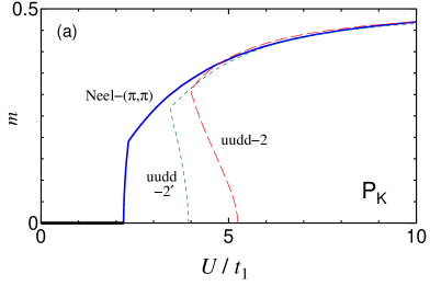
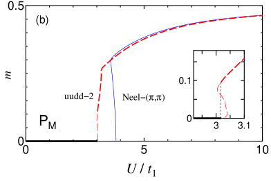
Figure 6: (Color online) Sublattice magnetizations for parameter sets (a) ${\rm P}_{\rm K}$ and (b) ${\rm P}_{\rm M}$. The blue solid, red dashed, and green short-dashed curves are the sublattice magnetizations $m$ for the Néel-$(\pi,\pi)$, uudd-2, and uudd-$2^{\prime}$ states, respectively. The thick and thin curves show the solutions with the lowest energy and those of the states with relatively higher energies, respectively. The black thick solid line of $m=0$ shows the paramagnetic state. In the inset of the lower panel (b), the vertical black thin dotted lines show the jump in $m$ at $U=U_{\rm c}$ between the uudd-2 and paramagnetic states.

(a)

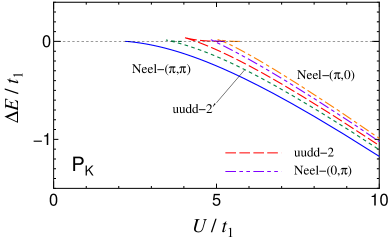
(b)

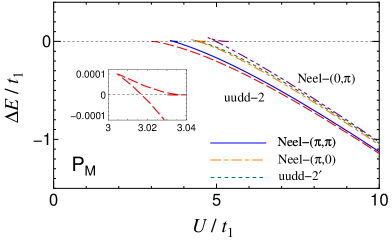
Figure 7: (Color online) Total energies of the five collinear phases near the quantum critical point for parameter sets (a) ${\rm P}_{\rm K}$ and (b) ${\rm P}_{\rm M}$. The blue solid, red dashed, green short-dashed, orange dot-dashed, and purple two-dot-dashed curves show $\Delta E$ of the Néel-$(\pi,\pi)$, uudd-2, uudd-$2^{\prime}$, Néel-$(\pi,0)$, and Néel-$(0,\pi)$ states, respectively.

3.2 Extending parameter region

In this subsection, we extend the range of the parameters.

3.2.1 Effect of the shift in $t_{3}$ and $r_{\rm imb}$ on $\Delta E(U)$

Figure 8 shows the value of $\Delta E(U)$ for ${\rm P}_{\rm K}^{\prime}$, in which $t_{3}=7.5\times 10^{-2}~{}{\rm eV}$. The critical value $U_{\rm c}$ for each magnetic structure is given by $\Delta E(U_{\rm c})=0$. The increase in $t_{3}$ results in an increase in $r_{\rm imb}$, i.e., the increase of the imbalance of the anisotropies. In contrast to ${\rm P}_{\rm K}$, for which the Néel-$(\pi,\pi)$ state is the ground state, the uudd-2 state becomes the ground state for ${\rm P}_{\rm K}^{\prime}$ as shown in Fig. 8(a). This figure also shows that the transition at $U_{\rm c}$ is of the second order. When $r_{\rm imb}$ increases, the energy of the Néel-$(\pi,\pi)$ state increases as shown in Fig. 8(b), whereas that of the uudd-2 state decreases in the close vicinity of $U_{\rm c}$; hence, $U_{\rm c}$ of the uudd-2 phase is slightly enhanced.

As a physical interpretation of the effect of the spatial-anisotropy imbalance, when the imbalance is large, the two types of bond triangles tend to have different frustrated spin structures; hence, the uudd states shown in Fig. 4 are favored more than the Néel states shown in Fig. 3. In particular, as $t_{3}$ increases, the exchange coupling constant $J_{3}\sim t_{3}^{2}/U$ increases, favoring an antiparallel configuration of the two spins on the sites connected by bond 3; hence, the uudd-2 state is more stabilized than the uudd-$2^{\prime}$ state, when $t_{3}$ is large.

(a)

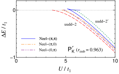
(b)

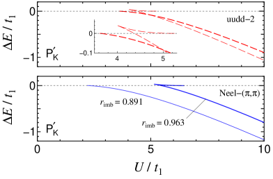
Figure 8: (Color online) Total energies for parameter set ${\rm P}_{\rm K}^{\prime}$ with $t_{3}=7.5\times 10^{-2}~{}{\rm eV}$, which leads to $r_{\rm imb}=0.963$. (a) The energies of the five collinear phases. (b) Comparison with the results for ${\rm P}_{\rm K}$, which are represented by the thin curves. For ${\rm P}_{\rm K}$, $r_{\rm imb}=0.891$. The legend is the same as that in Fig. 7.

(a)

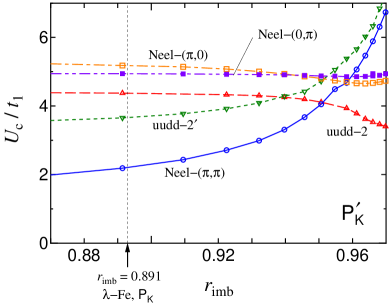
(b)

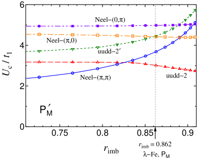
Figure 9: (Color online) $U_{\rm c}(r_{\rm imb})$ of the five collinear states for parameter sets (a) ${\rm P}_{\rm K}^{\prime}$ and (b) ${\rm P}_{\rm M}^{\prime}$, in which $t_{3}$ is variable. The open circles, open squares, closed squares, open triangles, and open inverted triangles are the results for the Néel-$(\pi,\pi)$, Néel-$(\pi,0)$, Néel-$(0,\pi)$, uudd-2, and uudd-$2^{\prime}$ states, respectively. The curves are guides to the eye.

(a)

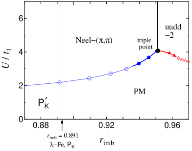
(b)

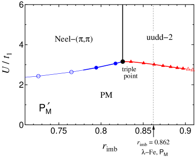
Figure 10: (Color online) Phase diagrams of the systems with parameter sets ${\rm P}_{\rm K}^{\prime}$ and ${\rm P}_{\rm M}^{\prime}$. The blue circles and red triangles are the points on the phase boundary of the Néel-$(\pi,\pi)$ phase and those between the uudd-2 and paramagnetic (PM) phases, respectively. The closed and open symbols indicate first-order and second-order transitions, respectively. The black thick solid lines show first-order transition lines between the Néel-$(\pi,\pi)$ and uudd-2 states. The blue and red curves are guides to the eye, where the thick and thin curves correspond to first- and second-order transitions, respectively. The large black closed circles show the triple points.

3.2.2 $U_{\rm c}(r_{\rm imb})$ and phase diagrams

Using parameter sets ${\rm P}_{\rm K}^{\prime}$ and ${\rm P}_{\rm M}^{\prime}$, in which $t_{3}$ is variable, we examine the influence of the shift in $r_{\rm imb}$. Figure 9 shows the behaviors of the critical values $U_{\rm c}$ of the five collinear states, below which their energies are higher than the energy of the paramagnetic state. The Néel-$(\pi,\pi)$ and uudd-2 states are suppressed and enhanced by the increase in $r_{\rm imb}$, respectively, which implies that the imbalance of the spatial anisotropies favors the uudd-2 state. The other collinear states, such as the Néel-$(\pi,0)$, Néel-$(0,\pi)$, and uudd-$2^{\prime}$ states, have higher energies in the present parameter ranges.

The phase diagrams in the $U$-$r_{\rm imb}$ plane are shown in Fig. 10. For both parameter sets ${\rm P}_{\rm K}^{\prime}$ and ${\rm P}_{\rm M}^{\prime}$, they contain areas of the Néel-$(\pi,\pi)$, uudd-2, and paramagnetic phases, and the uudd-2 phase occupies an area in which $r_{\rm imb}$ is large. The other collinear states do not appear in the parameter ranges of these figures. In both phase diagrams, a triple point of the two antiferromagnetic phases and the paramagnetic phase exists, near which all the transitions are of the first order. The phase boundary between the Néel-$(\pi,\pi)$ and uudd-2 states is parallel to the $U$-axis, and the transition is of the first order everywhere on the boundary. By contrast, the transitions from the two antiferromagnetic phases to the paramagnetic phase are of the second order when the system is far from the triple point. This feature is common to both ${\rm P}_{\rm K}^{\prime}$ and ${\rm P}_{\rm M}^{\prime}$.

The values of $r_{\rm imb}$ for the $\lambda$-Fe system are shown by the vertical thin dotted lines in Fig. 10. The increase in $U$ does not change the magnetic structure, provided that an antiferromagnetic state is the ground state within the present parameter ranges. By contrast, small changes in $r_{\rm imb}$ ($\Delta r_{\rm imb}\stackrel{{\scriptstyle{\textstyle>}}}{{\raisebox{-3.22916pt}{$\sim$}}}7\%$ for ${\rm P}_{\rm K}$ and $|\Delta r_{\rm imb}|\stackrel{{\scriptstyle{\textstyle>}}}{{\raisebox{-3.22916pt}{$\sim$}}}4\%$ for ${\rm P}_{\rm M}$) can change the magnetic structure.

4 Summary and Discussion

We examined the magnetic structure of electron systems on the ESCATL while focusing on the collinear states at $T=0$, and we adopted the Hubbard model and mean-field approximation. Within the parameter range, the Néel-$(\pi,\pi)$ state and a uudd state occur, and the transitions to these states can be of the first or second order depending on the parameters applied. The uudd states are favored under a large imbalance of the spatial anisotropies, which is a unique feature of the ESCATL, whereas the Néel-$(\pi,\pi)$ state occurs in wider parameter ranges. In the application to the $\lambda$-Fe system, we used candidate parameter sets ${\rm P}_{\rm K}$ and ${\rm P}_{\rm M}$. [10] As a result, it was found that for ${\rm P}_{\rm K}$, a second-order transition to the Néel-$(\pi,\pi)$ state occurs at $U_{\rm c}$, whereas for ${\rm P}_{\rm M}$, a first-order transition to the uudd-2 phase occurs at $U_{\rm c}$.

By extending parameter regions, we found triple points of the Néel-$(\pi,\pi)$, uudd-2, and paramagnetic phases, near which all transitions are of the first order. The transitions from the Néel-$(\pi,\pi)$ and uudd-2 phases to the paramagnetic phase are of the second order unless the system is close to the triple points both for ${\rm P}_{\rm K}^{\prime}$ and ${\rm P}_{\rm M}^{\prime}$. It should be examined in future research whether the existence of a triple point and the changes of the order of the transitions are universal features in the electron systems on the ESCATL.

For the $\lambda$-Fe system, the nesting vector $(\pi/c,0)$ obtained by previous studies suggests that the antiferromagnetic state has the modulation vector $(\pi/c,0)$ or $(\pi/c,\pi/a)$ as explained in Sect. 1. Between these states, the present result supports the antiferromagnetic state with $(\pi/c,\pi/a)$. In addition, the present study showed that the uudd phase can be the ground state of this system depending on the parameter values. The results are consistent with those in the classical spin system. [6]

In a previous study, the magnetic structure of the $\lambda$-Fe system was examined within a similar mean-field theory. [28] However, their model differs from our proposed model in many ways, resulting in discrepancies in the results. One of the significant differences between the two models lies in the lattice structures. In the previous model, the lattice site in the $\pi$-electron system corresponds to each BETS molecule, whereas in the present model, each dimer of the molecules is regarded as a lattice site. This results in a difference in the physical meaning of the on-site “$U$.” For example, $U$ in the previous model works only when the two electrons (or holes) are on the same BETS molecule, whereas the on-site $U$ in the present dimer model works when they are in the same dimer. Hence, the present $U$ includes an effect of the Coulomb repulsion between two electrons on different BETS molecules in the same dimer; however, such an interaction is ignored in the previous study. Thus, the effect of “$U$” must differ between the two models. For example, in the previous model, when $U$ increases, the system undergoes successive transitions, which were not found in the present study. The difference in the lattice structure also results in a difference in the filling of the relevant band having Fermi surfaces: In the present model, it is half-filled, which favors the insulating phase as observed in the $\lambda$-Fe system at low temperatures, whereas it is quarter-filled in the previous model. Meanwhile, the magnetic structure inside the dimer considered in the previous study is beyond the scope of this paper. The number of the sublattices in the mean-field approximation is different between the two theories. Another important difference is the presence of the 3d-spins: the previous model contains both $\pi$-electrons and 3d-spins, whereas we examined a pure $\pi$-electron system without d-spins on the basis of the current knowledge that the $\pi$-electron system is the principal component and the d-spins are passive in the exchange field created by the $\pi$-electrons. [30]

Although the phase diagrams do not contain the areas of the Néel-$(\pi,0)$ and Néel-$(0,\pi)$ states in the parameter regions examined in the present study, these states must occur depending on the parameters in the present itinerant system as well as in the classical localized spin system. Furthermore, although we neglected the spiral spin state, according to the experimental results [18, 19, 20, 21, 22, 23, 24] for the $\lambda$-Fe system, it may occur in other compounds including those that are yet undiscovered. A search for richer phase diagrams is a promising future research direction.

In the $\lambda$-Fe system, the magnetic long-range order is considered to be stabilized by the factors that originate from the d-spins of the ${\rm FeCl_{4}}$ anions, [34, 25, 35] such as the anisotropy in the spin space and/or the enhanced three dimensionality. As mentioned in Sect. 1, the present mean-field approximation implicitly assumes such factors. In future studies, improved theories beyond the mean-field approximation must explicitly incorporate these factors so that the stable magnetic long-range order in the $\lambda$-Fe system is reproduced.

It can be expected that the above results concerning the energies of the antiferromagnetic states are hardly affected by the d-spins, which are not incorporated in the present model, because the interactions in the $\pi$-electron system are much stronger than the other interactions (those in the d-spin system and those between the $\pi$-electrons and d-spins).

In conclusion, itinerant electron systems on the ESCATL as well as the localized spin system can exhibit uudd phases when the imbalance of the anisotropies is large. Within the parameter range examined, the transitions at $U_{\rm c}$ between the paramagnetic phase and the antiferromagnetic phase, such as the Néel-$(\pi,\pi)$ and uudd phases, are of the second order, except for a small parameter region near the junction of the three phase boundaries. Near the junction, all transitions are of the first order; hence, it is a triple point. The ground state of the $\lambda$-Fe system is most likely the Néel-$(\pi,\pi)$ state or a uudd state.

Appendix A Explicit forms of the matrices ${\hat{\cal E}}_{{{\bm{k}}}\sigma}$

This appendix shows the matrix elements of

$${\hat{\cal E}}_{{{\bm{k}}}\sigma}=\left(\begin{array}[]{cccc}{\tilde{\xi}}_{{{\bm{k}}}\sigma}^{\,\rm(AA)}&{\tilde{\xi}}_{{{\bm{k}}}}^{\,\rm(AA^{\prime})}&{\tilde{\xi}}_{{{\bm{k}}}}^{\,\rm(AB)}&{\tilde{\xi}}_{{{\bm{k}}}}^{\,\rm(AB^{\prime})}\\[4.0pt] {\tilde{\xi}}_{{{\bm{k}}}}^{\,\rm(A^{\prime}A)}&{\tilde{\xi}}_{{{\bm{k}}}\sigma}^{\,\rm(A^{\prime}A^{\prime})}&{\tilde{\xi}}_{{{\bm{k}}}}^{\,\rm(A^{\prime}B)}&{\tilde{\xi}}_{{{\bm{k}}}}^{\,\rm(A^{\prime}B^{\prime})}\\[4.0pt] {\tilde{\xi}}_{{{\bm{k}}}}^{\,\rm(BA)}&{\tilde{\xi}}_{{{\bm{k}}}}^{\,\rm(BA^{\prime})}&{\tilde{\xi}}_{{{\bm{k}}}\sigma}^{\,\rm(BB)}&{\tilde{\xi}}_{{{\bm{k}}}}^{\,\rm(BB^{\prime})}\\[4.0pt] {\tilde{\xi}}_{{{\bm{k}}}}^{\,\rm(B^{\prime}A)}&{\tilde{\xi}}_{{{\bm{k}}}}^{\,\rm(B^{\prime}A^{\prime})}&{\tilde{\xi}}_{{{\bm{k}}}}^{\,\rm(B^{\prime}B)}&{\tilde{\xi}}_{{{\bm{k}}}\sigma}^{\,\rm(B^{\prime}B^{\prime})}\end{array}\right).$$

The diagonal elements are common to all the five collinear states and expressed as

$${\tilde{\xi}}_{{{\bm{k}}}}^{(XX)}=-s_{X}s_{\sigma}Um-\mu,$$

where $X={\rm A},{\rm A^{\prime}},{\rm B}$, and ${\rm B^{\prime}}$. The off-diagonal elements ${\tilde{\xi}}_{{{\bm{k}}}}^{(XY)}=[{\tilde{\xi}}_{{{\bm{k}}}}^{(YX)}]^{*}$ are expressed as follows. For the Néel-$(\pi,\pi)$ state,

$$\begin{split}{\tilde{\xi}}_{{{\bm{k}}}}^{\,\rm(AB)}&={\tilde{\xi}}_{{{\bm{k}}}}^{\,\rm(A^{\prime}B^{\prime})}=2t_{1}\cos k_{x},\\ {\tilde{\xi}}_{{{\bm{k}}}}^{\,\rm(AB^{\prime})}&={\tilde{\xi}}_{{{\bm{k}}}}^{\,\rm(A^{\prime}B)}=t_{2}e^{-ik_{y}}+t_{2}^{\prime}e^{ik_{y}},\\ {\tilde{\xi}}_{{{\bm{k}}}}^{\,\rm(AA^{\prime})}&={\tilde{\xi}}_{{{\bm{k}}}}^{\,\rm(BB^{\prime})}=t_{3}e^{-i(k_{x}+k_{y})}+t_{3}^{\prime}e^{i(k_{x}+k_{y})}.\end{split}$$

For the Néel-$(\pi,0)$ state,

$$\begin{split}{\tilde{\xi}}_{{{\bm{k}}}}^{\,\rm(AB)}&={\tilde{\xi}}_{{{\bm{k}}}}^{\,\rm(A^{\prime}B^{\prime})}=2t_{1}\cos k_{x},\\ {\tilde{\xi}}_{{{\bm{k}}}}^{\,\rm(AA^{\prime})}&={\tilde{\xi}}_{{{\bm{k}}}}^{\,\rm(BB^{\prime})}=t_{2}e^{-ik_{y}}+t_{2}^{\prime}e^{ik_{y}},\\ {\tilde{\xi}}_{{{\bm{k}}}}^{\,\rm(AB^{\prime})}&={\tilde{\xi}}_{{{\bm{k}}}}^{\,\rm(BA^{\prime})}=t_{3}e^{-i(k_{x}+k_{y})}+t_{3}^{\prime}e^{i(k_{x}+k_{y})}.\\ \end{split}$$

For the Néel-$(0,\pi)$ state,

$$\begin{split}{\tilde{\xi}}_{{{\bm{k}}}}^{\,\rm(AA^{\prime})}&={\tilde{\xi}}_{{{\bm{k}}}}^{\,\rm(BB^{\prime})}=2t_{1}\cos k_{x},\\ {\tilde{\xi}}_{{{\bm{k}}}}^{\,\rm(AB)}&={\tilde{\xi}}_{{{\bm{k}}}}^{\,\rm(A^{\prime}B^{\prime})}=t_{2}e^{-ik_{y}}+t_{2}^{\prime}e^{ik_{y}},\\ {\tilde{\xi}}_{{{\bm{k}}}}^{\,\rm(AB^{\prime})}&={\tilde{\xi}}_{{{\bm{k}}}}^{\,\rm(BA^{\prime})}=t_{3}e^{-i(k_{x}+k_{y})}+t_{3}^{\prime}e^{i(k_{x}+k_{y})}.\\ \end{split}$$

For the uudd-2 state,

$$\begin{split}{\tilde{\xi}}_{{{\bm{k}}}}^{\,\rm(AB)}&={\tilde{\xi}}_{{{\bm{k}}}}^{\,\rm(A^{\prime}B^{\prime})}=2t_{1}\cos k_{x},\\ {\tilde{\xi}}_{{{\bm{k}}}}^{\,\rm(AA^{\prime})}&={\tilde{\xi}}_{{{\bm{k}}}}^{\,\rm(BB^{\prime})}=t_{2}e^{-ik_{y}}+t_{3}^{\prime}e^{i(k_{x}+k_{y})},\\ {\tilde{\xi}}_{{{\bm{k}}}}^{\,\rm(A^{\prime}B)}&={\tilde{\xi}}_{{{\bm{k}}}}^{\,\rm(B^{\prime}A)}=t_{2}^{\prime}e^{ik_{y}}+t_{3}e^{-i(k_{x}+k_{y})}.\\ \end{split}$$

For the uudd-$2^{\prime}$ state,

$$\begin{split}{\tilde{\xi}}_{{{\bm{k}}}}^{\,\rm(AB)}&={\tilde{\xi}}_{{{\bm{k}}}}^{\,\rm(A^{\prime}B^{\prime})}=2t_{1}\cos k_{x},\\ {\tilde{\xi}}_{{{\bm{k}}}}^{\,\rm(A^{\prime}B)}&={\tilde{\xi}}_{{{\bm{k}}}}^{\,\rm(B^{\prime}A)}=t_{2}e^{-ik_{y}}+t_{3}^{\prime}e^{i(k_{x}+k_{y})},\\ {\tilde{\xi}}_{{{\bm{k}}}}^{\,\rm(BB^{\prime})}&={\tilde{\xi}}_{{{\bm{k}}}}^{\,\rm(AA^{\prime})}=t_{2}^{\prime}e^{-ik_{y}}+t_{3}e^{i(k_{x}+k_{y})}.\\ \end{split}$$

References

- [1] L. Balents, Nature 464, 199 (2010), and references therein.
- [2] K. Kanoda and R. Kato, Annu. Rev. Condens. Matter Phys. 2, 167 (2011), and references therein.
- [3] P. Hauke, Phys. Rev. B 87, 014415 (2013).
- [4] S. Gopalan, T. M. Rice, and M. Sigrist, Phys. Rev. B 49, 8901 (1994).
- [5] A. H. Castro Neto, F. Guinea, N. M. R. Peres, K. S. Novoselov, and A. K. Geim, Rev. Mod. Phys. 81, 109 (2009).
- [6] K. Sakakida and H. Shimahara, J. Phys. Soc. Jpn. 86, 124709 (2017).
- [7] BETS represents bis(ethylenedithio)tetraselenafulvalene.
- [8] This fact was suggested by the results of the specific heat measurements. [30, 21]
- [9] T. Mori and M. Katsuhara, J. Phys. Soc. Jpn. 71, 826 (2002).
- [10] The values of the transfer integrals obtained by Kobayashi and Mori are presented in Ref. \citenHot00. Their results do not coincide; however, because explicit physical conditions assumed for their calculations are not presented, the reason for the difference is unknown. We adopt them as candidates for the parameters of the -Fe system.
- [11] BEDT-STF represents bis(ethylenedithio)dithiadiselenafulvalene. The compound -- has been studied by many authors; for example, [S. Fukuoka, T. Minamidate, N. Matsunaga, Y. Ihara, and A. Kawamoto, J. Phys. Soc. Jpn. 89, 073704 (2020)], and references therein.
- [12] BEST represents bis(ethylenediseleno)tetrathiafulvalene. For the compound -, see [H. B. Cui, S. Otsubo, Y. Okano, and H. Kobayashi, Chemistry Letters 34, 254 (2005)].
- [13] M. Roger, J. M. Delrieu, and J. H. Hetherington, Phys. Rev. Lett. 45, 137 (1980).
- [14] T. Kimura, S. Ishihara, H. Shintani, T. Arima, K. T. Takahashi, K. Ishizaka, and Y. Tokura, Phys. Rev. B 68, 060403(R) (2003).
- [15] A. Muñoz, M. T. Casáis, J. A. Alonso, M. J. Martínez-Lope, J. L. Martínez, and M. T. Fernández-Díaz, Inorg. Chem. 40, 1020 (2001).
- [16] T. A. Kaplan, Phys. Rev. B 80, 012407 (2009).
- [17] T. Zou, Y.-Q. Cai, C. R. dela Cruz, V. O. Garlea, S. D. Mahanti, J.-G. Cheng, and X. Ke, Phys. Rev. B 94, 214406 (2016).
- [18] Y. Oshima, H.-B. Cui, and R. Kato, Magnetochemistry 3, 10 (2017).
- [19] T. Sasaki, H. Uozaki, S. Endo, and N. Toyota, Synth. Met. 120, 759 (2001).
- [20] M. Tokumoto, H. Tanaka, T. Otsuka, H. Kobayashi, and A. Kobayashi, Polyhedron 24, 2793 (2005).
- [21] H. Akiba, K. Nobori, K. Shimada, Y. Nishio, K. Kajita, B. Zhou, A. Kobayashi, and H. Kobayashi, J. Phys. Soc. Jpn. 80, 063601 (2011).
- [22] A. Sato, E. Ojima, H. Akutsu, H. Kobayashi, A. Kobayashi, and P. Cassoux, Chem. Lett. 27, 673 (1998).
- [23] M. Tokumoto, T. Naito, H. Kobayashi, V. N. Laukhin, L. Brossard, and P. Cassoux, Synth. Met. 86, 2161 (1997).
- [24] K. Ito and H. Shimahara, J. Phys. Soc. Jpn. 85, 024704 (2016).
- [25] H. Shimahara and Y. Kono, J. Phys. Soc. Jpn. 86, 043704 (2017).
-
[26]
An argument in Ref. \citenShi17 suggests that
the -Fe system
is close to the quantum critical point
().
A simple analysis leads to the expression of
the antiferromagnetic transition temperature
in the mixed crystal -:
where is the magnitude of the d-spin, and is the exchange coupling constant between the -electrons and the d-spins. This expression explains the experimental observations that . From the experimental observation that , it follows that . - [27] L. Brossard, R. Clerac, C. Coulon, M. Tokumoto, T. Ziman, D. K. Petrov, V. N. Laukhin, M. J. Naughton, A. Audouard, F. Goze, A. Kobayashi, H. Kobayashi, and P. Cassoux, Eur. Phys. J. B 1, 439 (1998).
- [28] C. Hotta and H. Fukuyama, J. Phys. Soc. Jpn. 69, 2577 (2000).
- [29] M. Terao and Y. Ohashi, Physica C 412–414, 324 (2004).
- [30] H. Akiba, S. Nakano, Y. Nishio, K. Kajita, B. Zhou, A. Kobayashi, and H. Kobayashi, J. Phys. Soc. Jpn. 78, 033601 (2009).
- [31] H. Kobayashi, A. Sato, H. Tanaka, A. Kobayashi, and P. Cassoux, Coordination Chem. Rev. 190–192, 921 (1999).
- [32] A. Sato, E. Ojima, H. Akutsu, Y. Nakazawa, H. Kobayashi, H. Tanaka, A. Kobayashi, and P. Cassoux, Phys. Rev. B 61, 114 (2000).
- [33] H. Akiba, H. Sugawara, K. Nobori, K. Shimada, N. Tajima, Y. Nishio, K. Kajita, B. Zhou, A. Kobayashi, and H. Kobayashi, J. Phys. Soc. Jpn. 81, 053601 (2012).
- [34] H. Shimahara and K. Ito, J. Phys. Soc. Jpn. 83, 114702 (2014).
- [35] H. Shimahara, J. Phys. Soc. Jpn. 87, 043702 (2018).
- [36] The term in Eq. (2) cannot be eliminated by an appropriate choice of the origin of the energy; omitting the term in the evaluation of leads to unphysical results. See the argument below Eq. (4).