Path-integral calculation of the third dielectric virial coefficient of noble gases

Abstract

We present the first framework for fully quantum calculation of the third dielectric virial coefficient $C_{\varepsilon}(T)$ of noble gases, including exchange effects. The quantum effects are taken into account with the path-integral Monte Carlo method. Calculations employing state-of-the-art pair and three-body potentials and pair polarizabilities yield results generally consistent with the few scattered experimental data available for helium, neon, and argon, but rigorous calculations with well-described uncertainties will require the development of surfaces for the three-body nonadditive polarizability and the three-body dipole moment. The framework developed here will enable new approaches to primary temperature and pressure metrology based on first-principles calculations of gas properties.

I Introduction

Just as the deviation of a gas’s thermodynamic behavior from that of an ideal gas is described by the familiar virial expansion, the dielectric virial expansion describes the low-density behavior of the static dielectric constant $\varepsilon$. The Clausius–Mossotti function for a low-density gas of identical molecules can be expanded in powers of molar density $\rho$ as:

$$\frac{\varepsilon-1}{\varepsilon+2}=\rho\left(A_{\varepsilon}+B_{\varepsilon}\rho+C_{\varepsilon}\rho^{2}+\ldots\right)=\rho A_{\varepsilon}\left(1+b\rho+c\rho^{2}+\ldots\right)\ ,$$ (1)

where for non-polar molecules $A_{\varepsilon}$ is proportional to the trace of the static polarizability of the isolated molecule. Both the lower-case and upper-case coefficients in Eq. (1) are sometimes called “dielectric virial coefficients” in the literature; in this work we use the upper-case quantities where $B_{\varepsilon}$ is the second dielectric virial coefficient, $C_{\varepsilon}$ is the third dielectric virial coefficient, etc.

The dielectric virial expansion has seen increasing use in precision metrology, particularly for fundamental measurements of pressure and of the thermodynamic temperature. For example, in dielectric-constant gas thermometry,Gaiser, Zandt, and Fellmuth (2015); Gaiser, Fellmuth, and Haft (2017); Gaiser et al. (2017); Gaiser, Fellmuth, and Haft (2020) capacitance measurements on noble gases (where the dielectric virial coefficients are relatively small) are able to determine the thermodynamic temperature with uncertainties smaller than 1 mK. Another example is a primary pressure standard up to 7 MPa based on measuring the static dielectric constant of helium;Gaiser, Fellmuth, and Sabuga (2020) the uncertainty in $C_{\varepsilon}$ was one of the two largest contributors to the uncertainty budget of the standard. A related expansion for the refractivity is also used in refractive-index gas thermometry, and in most implementations the frequency is close enough to the static limit that the appropriate coefficients to use are those in the dielectric virial expansion, with an additional term proportional to the magnetic susceptibility.Piszczatowski et al. (2015); Rourke et al. (2019); Gao et al. (2020); Madonna Ripa et al. (2021); Rourke (2021) When the static limit is not accurate enough – e.g., for refractive-index gas metrology at optical frequencies – the frequency dependence of the coefficients in Eq. (1) is also required. Piszczatowski et al. (2015); Garberoglio and Harvey (2020a)

Particularly in the case of helium where the polarizability of the isolated atom (and therefore $A_{\varepsilon}$) can be calculated with extraordinary accuracy,Puchalski et al. (2020) much of the interest lies in first-principles calculations of the virial coefficients in order to allow, for example, calculation of pressure from a dielectric measurement without any need for external calibration.

The second dielectric virial coefficient $B_{\varepsilon}$ depends only on temperature for a given fluid; for monatomic species it can be calculated from the interatomic potential-energy curve and the nonadditive two-body polarizability. Similarly, $C_{\varepsilon}$ requires knowledge of the three-body potential, the three-body polarizability, and the three-body dipole moment. While the classical calculation of $B_{\varepsilon}$, and to a lesser extent $C_{\varepsilon}$, is fairly straightforward if the potentials, polarizabilities and the dipole moment are known, helium is light enough that quantitative accuracy requires the inclusion of quantum effects, and at low temperature quantum effects can be significant for neon and to a lesser extent argon.

Recently, we reported fully quantum calculations of the second dielectric and refractivity virial coefficients of helium, neon, and argon based on state-of-the-art pair potentials and pair polarizabilities.Garberoglio and Harvey (2020a) The calculations were performed with the venerable wavefunction-based method for quantum two-body problems,Hirschfelder, Curtiss, and Bird (1954) but the work also introduced a path-integral approach for the quantum calculation of $B_{\varepsilon}$, showing that the two independent approaches agreed (they also agreed with semiclassical resultsSong and Luo (2020) at the high and moderate temperatures where the semiclassical approach to quantum effects is valid). The advantage of the path-integral approach is that, just as in the case of the thermodynamic third virial coefficient,Garberoglio and Harvey (2009); Garberoglio, Moldover, and Harvey (2011) it can be extended to compute the third dielectric virial coefficient where no exact quantum solution is known.

The extension of the path-integral method to the quantum calculation of $C_{\varepsilon}$ is the main topic of this paper. After a review of previous calculations, we will present a derivation of the dielectric virial expansion, including expressions for $B_{\varepsilon}$ and $C_{\varepsilon}$. We will then derive a path-integral formulation for $C_{\varepsilon}$, which will include all quantum effects, including exchange. Calculations will then be performed for ⁴He, neon, and argon, and comparisons will be made with the limited experimental data available.

II Previous Calculations

The only previous attempt to calculate $C_{\varepsilon}$ completely from first principles was in a 1974 paper by Heller and Gelbart,Heller and Gelbart (1974) who reported a value of $-0.716\text{\,}~{}$cm⁹ mol^-3 for helium at “room temperature.” This value has been used, either by itself or in combination with reported experimental values, in many metrology applications,Puchalski et al. (2016); Rourke (2017); Gaiser and Fellmuth (2019); Gao et al. (2020); Gaiser, Fellmuth, and Sabuga (2020) including some that are not near room temperature. However, there are several problems with general use of the value of Heller and Gelbart:

• It ignores temperature dependence of $C_{\varepsilon}$. There is a large temperature dependence both for helium’s thermodynamic third virial coefficientGarberoglio, Moldover, and Harvey (2011) and its second dielectric virial coefficient.Garberoglio and Harvey (2020a) Assuming $C_{\varepsilon}$ to be independent of temperature is clearly unjustified.

• It is an entirely classical calculation. This should not introduce much error for applications near room temperature, but quantum effects are likely to be significant at cryogenic temperatures.

• The input to the calculation was primitive by today’s standards. For simplicity, Heller and Gelbart assumed the intermolecular potential to be that of a hard sphere. The pair polarizability was taken from a 1973 paperO’Brien et al. (1973) that used a relatively low level of theory by modern standards. The three-body potential was assumed to be zero, and the three-body polarizability was approximated in a simple way.

The 1980 paper of Alder et al.Alder et al. (1980) contains values of $C_{\varepsilon}$ calculated classically for helium and argon, but upon closer inspection it is evident that a parameter in the pair polarizability for each substance was arbitrarily adjusted to obtain agreement with some experimental data. We note that the sources of experimental data they usedVidal and Lallemand (1976); Lallemand and Vidal (1977) report values of $B_{\varepsilon}$ that are inconsistent with recent results for helium, neon, and argon.Garberoglio and Harvey (2020a)

These two calculational papers approximated the three-body polarizability with somewhat different versions of a “superposition approximation,” stated to be valid in the limit of large separations. The form of this approximation will be discussed further in Section III.4.

III The virial expansion of the dielectric constant

In the literature, one can find several mutually incompatible expressions for $C_{\varepsilon}(T)$ Hill (1958); Moszynski, Heijmen, and van der Avoird (1995); Gray, Gubbins, and Joslin (2011). In the following, we will present the correct one, highlighting similarities and points of departure from the others.

III.1 Electric fields and polarization in homogeneous isotropic media

We consider a region of volume $V$ in a quantum gas of identical polarizable particles subject to an externally applied electric field (generated, for example, by a distribution $\varrho(\mathbf{x})$ of electric charges on some external conductors). Let us denote by $\mbox{\boldmath$E$}_{0}$ the electric field in the region $V$ coming from the sum of the electric field generated by $\varrho(\mathbf{x})$ and the polarization of the gas external to the volume $V$. We assume that the volume $V$ contains enough particles to justify a statistical description (that is, temperature and chemical potential can be defined), but small enough to neglect the spatial variation of $\mbox{\boldmath$E$}_{0}$ within it. We further assume that we deal with a linear dielectric, that is the electric field is everywhere weak enough so that the polarization density $P$ within $V$, defined as the dipole moment per unit of volume, depends linearly on the applied field. The dielectric constant $\varepsilon$ (the relative electric permittivity) for this system is defined by the relation Jackson (1998)

$$\mbox{\boldmath$P$}=\frac{\varepsilon-1}{4\pi}\mbox{\boldmath$E$},$$ (2)

where $E$ is the macroscopic electric field in the medium (the Maxwell field). This definition is equivalent to the statement that $\mbox{\boldmath$D$}=\varepsilon\mbox{\boldmath$E$}$, where $\mbox{\boldmath$D$}=\mbox{\boldmath$E$}+4\pi\mbox{\boldmath$P$}$ is the electric displacement (electric induction). Jackson (1998) In this case, $E$ is the sum of the field $\mbox{\boldmath$E$}_{0}$ and the average value of the field generated by the polarized medium within $V$. As the dielectric constant is independent on the shape of the arbitrarily chosen small volume $V$, we can assume that $V$ is spherical. In this case, the latter field is equal to $-(4\pi/3)\mbox{\boldmath$P$}$, Jackson (1998) and we have

$$\mbox{\boldmath$\ E$}=\mbox{\boldmath$E$}_{0}-\frac{4\pi}{3}\mbox{\boldmath$P$}.$$ (3)

Combining Eq. (2) with Eq. (3) leads to

$$\mbox{\boldmath$P$}=\frac{3}{4\pi}\,\frac{\varepsilon-1}{\varepsilon+2}\,\mbox{\boldmath$E$}_{0}.$$ (4)

At the end of the calculation, we can take the thermodynamic limit $V\rightarrow\infty$, and our system becomes equivalent to an infinite homogeneous gas in an external field $\mbox{\boldmath$E$}_{0}$, i.e., we neglect any boundary effects. For an atomic gas, the vectors $\mbox{\boldmath$E$}_{0}$, $P$, $E$, and $D$ are parallel so that $\mbox{\boldmath$E$}_{0}$=$E_{0}\mbox{\boldmath$k$}$, $P$=$P\mbox{\boldmath$k$}$, $E$=$E\mbox{\boldmath$k$}$, and $D$=$D\mbox{\boldmath$k$}$, where $k$ is the unit vector parallel to the external field $\mbox{\boldmath$E$}_{0}$.

III.2 Quantum statistical mechanics of the dielectric response

In view of Eq. (4) and Eq. (1), the dielectric viral coefficients can be obtained by expanding $4\pi P/(3E_{0})$ in powers of particle number density $\rho$. Application of classical Hill (1958) or quantum Garberoglio et al. statistical mechanics results in the following expansion for $P$

$$P=\alpha_{1}\rho E_{0}-k_{\mathrm{B}}T\sum_{n=2}^{\infty}\left(\frac{1}{n-1}\right)\left.\frac{\partial B_{n}(T,E_{0})}{\partial E_{0}}\right|_{E_{0}=0}\rho^{n},$$ (5)

where $\alpha_{1}$ is the atomic polarizability, $T$ is the temperature, and $B_{n}(T,E_{0})$ is the usual $n$th density virial coefficient for an infinite system in the external static and uniform electric field of magnitude $E_{0}$.

It should be noted that the formula for $P$ given by Eq. (24) in Ref. Hill, 1958 is formally identical with Eq. (5) except that the external field strength $E_{0}$ is replaced by the electric displacement $D$, which leads to incorrect expressions for the second and higher dielectric virial coefficients.

The density virials $B_{n}(T,E_{0})$ are given as the $V\to\infty$ combinations of the functions $Z_{N}(V,T,E_{0})$ defined as

$$\frac{Z_{N}(T,E_{0})}{N!}=\frac{Q_{N}(V,T,E_{0})V^{N}}{Q_{1}(V,T,E_{0})^{N}},$$ (6)

where $Q_{N}(V,T,E_{0})$ are the canonical partition functions of $N$ particles in volume $V$ in the presence of an external uniform electric field of magnitude $E_{0}$. In classical mechanics, $Q_{N}(V,T,E_{0})$ is the phase integral over the Boltzmann factor $\mathrm{e}^{-\beta H(V,N,E_{0})}$ divided by $N!h^{3N}$, where $\beta=1/k_{\mathrm{B}}T$, $h$ is the Planck constant, and $H(V,N,E_{0})$ is the classical Hamiltonian of the system. In quantum mechanics, $Q_{N}(V,T,E_{0})$ is the trace of the Boltzmann operator $\mathrm{e}^{-\beta H(V,N,E_{0})}$ in the bosonic or fermionic Hilbert space, where now $H(V,N,E_{0})$ stands for the quantum Hamiltonian. In particular, one has Hirschfelder, Curtiss, and Bird (1954)

$$B_{2} = -\frac{1}{2V}\left(Z_{2}-V^{2}\right)$$ (7)

$$B_{3} = \frac{\left(Z_{2}-V^{2}\right)^{2}}{V^{2}}-\frac{1}{3V}\left(Z_{3}-3Z_{2}V+2V^{3}\right).$$ (8)

Since the derivation of Eq. (5) has been performed in the grand canonical ensemble, we think of the volume $V$ as a part of the volume of an experimental apparatus. We assume that $V$ is large enough to contain enough atoms to fulfill the requirements of the thermodynamic limit. Notice that the quantities $B_{n}(T,E_{0})$ are finite in the usual $V\rightarrow\infty$ limit.

We now follow Moszynski et al. Moszynski, Heijmen, and van der Avoird (1995) and substitute in Eq. (5) the equivalence

$$\frac{\partial B_{n}(T,E_{0})}{\partial E_{0}}=\frac{\partial^{2}B_{n}(T,E_{0})}{\partial^{2}E_{0}}E_{0},$$ (9)

which is valid in the $E_{0}\to 0$ limit since $B_{n}(T,E_{0})$ depends quadratically on $E_{0}$,Hill (1958) thus obtaining

$$\frac{P}{E_{0}}=\alpha_{1}\rho-k_{\mathrm{B}}T\sum_{n=2}^{\infty}\left(\frac{1}{n-1}\right)\frac{\partial^{2}B_{n}(T,E_{0})}{\partial^{2}E_{0}}\rho^{n}.$$ (10)

Recalling Eq. (4), we finally arrive at

$$\frac{\varepsilon-1}{\varepsilon+2} = \frac{4\pi}{3}\left[\alpha_{1}\rho-k_{\mathrm{B}}T\sum_{n=2}^{\infty}\left(\frac{1}{n-1}\right)\frac{\partial^{2}B_{n}(T,E_{0})}{\partial^{2}E_{0}}\rho^{n}\right]$$ (11)

$$\equiv A_{\varepsilon}\rho+B_{\varepsilon}\rho^{2}+C_{\varepsilon}\rho^{3}+\ldots$$ (12)

$$A_{\varepsilon} = \frac{4\pi\alpha_{1}}{3}$$ (13)

$$B_{\varepsilon} = \frac{2\pi k_{\mathrm{B}}T}{3V}\frac{\partial^{2}Z_{2}(V,T,E_{0})}{\partial E_{0}^{2}}$$ (14)

$$C_{\varepsilon} = -\frac{2\pi k_{\mathrm{B}}T}{3}\left[\frac{2}{V^{2}}\left(\frac{\partial Z_{2}}{\partial E_{0}}\right)^{2}+\frac{2(Z_{2}-V^{2})}{V^{2}}\frac{\partial^{2}Z_{2}}{\partial E_{0}^{2}}\right.+$$ (15)

$$\left.-\frac{1}{3V}\left(\frac{\partial^{2}Z_{3}}{\partial E_{0}^{2}}-3V\frac{\partial^{2}Z_{2}}{\partial E_{0}^{2}}\right)\right]$$

which is the virial expansion that we will use in this paper, with the coefficients defined in Eq. (12). Keeping the lowest term in $\rho$ recovers the Clausius–Mossotti equation, whereas the coefficient of the term $\rho^{2}$ that we obtain is in perfect agreement with the results reported in Refs. Moszynski, Heijmen, and van der Avoird, 1995 and Gray, Gubbins, and Joslin, 2011.

As already mentioned our expression for $P$, and consequently for the dielectric virial coefficients differs from that of Hill Hill (1958). In fact, his expression for $P$ is incorrect even for the ideal gas as it does not lead to the Clausius– Mossotti equation in this case, see Eqs. (32)-(34) in Ref. Hill, 1958. In a later paper, Hill (1959) Hill proposed to correct his expression for $P$ by substituting the Maxwell field $E$ for the electric displacement $D$. The resulting expression for $P$ remains incorrect.

Although we obtain the same formula for $B_{\varepsilon}$ as Moszynski et al., Moszynski, Heijmen, and van der Avoird (1995) our expression for $C_{\varepsilon}$ differs from theirs, because they mistakenly use Eq. (2) with $E=E_{0}$ in all the terms of the right-hand side of Eq. (5) except the first, for which their considerations are equivalent to ours. Finally, we notice that our expression for the third dielectric virial coefficient is equivalent, in the classical limit, to the one derived in Ref. Gray, Gubbins, and Joslin, 2011. Equation (15) can also be obtained starting from the fundamental equations of quantum statistical mechanics, and we will present this alternative derivation in a forthcoming work. Garberoglio et al.

III.3 Hamiltonians in an external field

In the case of polarizable atoms, the partition functions $Q_{N}(V,T,E_{0})$ appearing in Eq. (6) are obtained using an $N$-particle Hamiltonian function $H(N)=H_{0}(N)+\Delta H_{1}(N)+\Delta H_{2}(N)$, which is the sum of the Hamiltonian $H_{0}(N)$ of $N$ atoms without the external field plus two contributions $\Delta H_{1}(N)$ and $\Delta H_{2}(N)$ describing the linear and quadratic interaction with the external field, respectively (terms with higher order in $\mathbf{E}_{0}$ do not contribute to the dielectric constant). These three functions are given by

$$H_{0}(N) = \sum_{i=1}^{N}\frac{\bm{\pi}_{i}^{2}}{2m}+\sum_{i<j}u_{2}(i,j)+\sum_{i<j<k}u_{3}(i,j,k)+\ldots,$$ (16)

$$\Delta H_{1}(N) = -\left(\sum_{i=1}^{N}\mathbf{m}_{1}(i)+\sum_{i<j}\mathbf{m}_{2}(i,j)+\right.$$ (17)

$$\left.\sum_{i<j<k}\mathbf{m}_{3}(i,j,k)+\ldots\right)\cdot\mathbf{E}_{0}$$

$$\Delta H_{2}(N) = -\frac{1}{2}\mathbf{E}_{0}\cdot\left(\sum_{i=1}^{N}\bm{\alpha}_{1}(i)+\sum_{i<j}\bm{\alpha}_{2}(i,j)+\right.$$ (18)

$$\left.\sum_{i<j<k}\bm{\alpha}_{3}(i,j,k)+\ldots\right)\cdot\mathbf{E}_{0},$$

where $m$ is the mass of the atoms, $\bm{\pi}_{i}$ is the momentum of the $i$-th atom, $u_{k}(1,\ldots,k)$ is the irreducible $k$-body potential, $\mathbf{m}_{k}(1,\ldots,k)$ is the dipole moment and $\bm{\alpha}_{k}(1,\ldots,k)$ is the $k$-body induced polarizability, which is a $3\times 3$ matrix. For noble gases, $\mathbf{m}_{1}(i)$ and $\mathbf{m}_{2}(i,j)$ are identically zero, but a configuration of three atoms can have a permanent dipole, hence $\mathbf{m}_{3}(i,j,k)$ is in general not zero. Martin (1974); Bruch, Corcoran, and Weinhold (1978)

III.4 The induced-dipole–induced-dipole model for the polarizability

In general, the quantities $\mathbf{m}_{k}(1,\ldots,k)$ and $\bm{\alpha}_{k}(1,\ldots,k)$ appearing in Eqs. (17) and (18) must be obtained by ab initio calculations of the ground-state energy of a cluster of $n$ atoms in the presence of an external field. Presently, only $\bm{\alpha}_{2}$ is known with sufficient precision to enable highly accurate calculations of $B_{\varepsilon}$ Garberoglio and Harvey (2020a) for helium, neon, and argon. In the case of $\mathbf{m}_{3}$, a first-principles parameterization for noble gases, valid in the limit of large distances, has been developed by Li and Hunt. Li and Hunt (1997) Its accuracy is unknown, but as will be discussed in Sec. V, the contribution of $\mathbf{m}_{3}$ to $C_{\varepsilon}(T)$ appears to be relatively small.

To the best of our knowledge, no first-principles surface for $\bm{\alpha}_{3}$ has been published in the literature. As we will discuss below, the contribution from the three-body polarizability to $C_{\varepsilon}(T)$ turns out to be substantial and for this reason it is worthwhile to briefly investigate models for the polarizability that lead to approximate expressions for $\bm{\alpha}_{3}$ as a function of the lower-order polarizabilities. One of the most used models assumes that the dipole moment $\mathbf{p}_{i}$ of atom $i$ depends on the the total field acting on it

$$\mathbf{p}_{i}=\alpha_{1}\mathbf{E}_{\mathrm{tot}}(\mathbf{r}_{i}),$$ (19)

and that the total field is given by the sum of the externally applied field $\mathbf{E}_{0}$ and the contribution of the fields generated by the induced dipoles

$$\mathbf{E}_{\mathrm{tot}}(\mathbf{r}_{i})=\mathbf{E}_{0}+\sum_{j\neq i}\mathsf{T}(\mathbf{r}_{i}-\mathbf{r}_{j})\mathbf{p}_{j}(\mathbf{r}_{j}),$$ (20)

where the tensor $\mathsf{T}(\mathbf{r})$ is given by

$$\mathsf{T}_{\alpha\beta}(\mathbf{r})=\frac{3r_{\alpha}r_{\beta}}{r^{5}}-\frac{\delta_{\alpha\beta}}{r^{3}},$$ (21)

where $r_{\alpha}$ is the $\alpha$-th component of the vector $\mathbf{r}$.

The solution of these equations in the case of three particles Buckingham and Hands (1991) shows that one has

$$\bm{\alpha}_{2}(\mathbf{r}_{1},\mathbf{r}_{2}) \simeq 2\alpha_{1}^{2}\mathsf{T}(\mathbf{r}_{12})$$ (22)

$$\bm{\alpha}_{3}(\mathbf{r}_{1},\mathbf{r}_{2},\mathbf{r}_{3}) \simeq 2\alpha_{1}^{3}\left[\mathsf{T}(\mathbf{r}_{12})\mathsf{T}(\mathbf{r}_{23})+\right.$$ (23)

$$\mathsf{T}(\mathbf{r}_{23})\mathsf{T}(\mathbf{r}_{31})+$$

$$\left.\mathsf{T}(\mathbf{r}_{31})\mathsf{T}(\mathbf{r}_{12})\right],$$

where we have defined $\mathbf{r}_{ij}=\mathbf{r}_{i}-\mathbf{r}_{j}$. The last result can be generalized by the so-called superposition approximation Gelbart (1974); Heller and Gelbart (1974); Alder et al. (1980) for $\bm{\alpha}_{3}$ as a function of $\bm{\alpha}_{2}$,

$$\bm{\alpha}_{3}(\mathbf{r}_{1},\mathbf{r}_{2},\mathbf{r}_{3})=\frac{1}{2\alpha_{1}}\left[\bm{\alpha}_{2}(1,2)\bm{\alpha}_{2}(2,3)+\bm{\alpha}_{2}(2,3)\bm{\alpha}_{2}(3,1)+\bm{\alpha}_{2}(3,1)\bm{\alpha}_{2}(1,2)\right],$$ (24)

where we denoted $\bm{\alpha}_{2}(i,j)=\bm{\alpha}_{2}(\mathbf{r}_{i},\mathbf{r}_{j})$. Similar approximations appeared in the literature: Heller and Gelbart Heller and Gelbart (1974) approximated the $zz$ component of $\bm{\alpha}_{3}$ similarly to Eq. (24), but considered it as given by the product of the $zz$ components of the two $\bm{\alpha}_{2}$ tensors, and did not consider the factor of $1/2$. Our definition of the superposition approximation is the same as that used by Alder et al.Alder et al. (1980) Equation (24) agrees asymptotically at large interatomic distances with the exact asymptotics of the three-body polarizability derived by Champagne et al. Champagne, Li, and Hunt (2000)

III.5 Structure of the pair and three-body polarizabilities

In general, the pair polarizability $\bm{\alpha}_{2}(\mathbf{r})$ is written as

$$\bm{\alpha}_{2}(\mathbf{r})_{\alpha\beta}=\alpha_{\mathrm{iso}}(r)\delta_{\alpha\beta}+\frac{\alpha_{\mathrm{aniso}}(r)}{3}\mathsf{t}_{\alpha\beta}(\mathbf{r})$$ (25)

where $\mathsf{t}_{\alpha\beta}(\mathbf{r})=r^{3}\mathsf{T}_{\alpha\beta}(\mathbf{r})$. The quantity $\alpha_{\mathrm{iso}}(r)$ and $\alpha_{\mathrm{aniso}}(r)$ are known as the average trace of the pair-induced polarizability and the anisotropic component, respectively. As we will see below, the relevant quantities involved in the calculation of the dielectric virial coefficients are the traces of $\bm{\alpha}_{n}$ defined in Eq. (18). A straightforward calculation using Eqs. (25) and (24) shows that

$$\frac{1}{3}\mathrm{tr}\left[\bm{\alpha}_{3}(r_{12},r_{13},r_{23})\right] = \frac{1}{2\alpha_{1}}\left[\alpha_{\mathrm{iso}}(r_{12})\alpha_{\mathrm{iso}}(r_{23})+\frac{\alpha_{\mathrm{aniso}}(r_{12})\alpha_{\mathrm{aniso}}(r_{23})}{3}\left(\cos^{2}\theta_{2}-\frac{1}{3}\right)+\right.$$ (26)

$$\alpha_{\mathrm{iso}}(r_{13})\alpha_{\mathrm{iso}}(r_{32})+\frac{\alpha_{\mathrm{aniso}}(r_{13})\alpha_{\mathrm{aniso}}(r_{32})}{3}\left(\cos^{2}\theta_{3}-\frac{1}{3}\right)+$$

$$\left.\alpha_{\mathrm{iso}}(r_{12})\alpha_{\mathrm{iso}}(r_{13})+\frac{\alpha_{\mathrm{aniso}}(r_{12})\alpha_{\mathrm{aniso}}(r_{13})}{3}\left(\cos^{2}\theta_{1}-\frac{1}{3}\right)\right],$$

where $\theta_{i}$ is the angle at particle $i$ in the triangle having as vertices the three particles considered.

IV The path-integral formulation

In general, the partition functions involved in the definition of $Z_{N}$ (see Eq. (6)) can be written as

$$Q_{N}(V,T,E_{0})=\frac{1}{N!}\sum_{i,\sigma}\langle i|\mathrm{e}^{-\beta H(N)}P_{\sigma}|i\rangle,$$ (27)

where the states $|i\rangle$ denote a complete basis set in the Hilbert space of $N$ atoms, $\sigma$ are permutations of $N$ objects, and $P_{\sigma}$ is the operator representing the permutation in the Hilbert space, weighted with the sign of the permutation in the case of fermions. At high temperatures, when the de Broglie thermal wavelength $\Lambda=h/\sqrt{2mk_{\mathrm{B}}T}$ is much smaller than the hard-core radius of the atoms, only the term where $\sigma$ is the identity permutations contributes to Eq. (27). In this case, the bosonic or fermionic nature of the quantum particles is not apparent and particles behave as distinguishable (Boltzmann limit); quantum effects appear only as a consequence of Heisenberg uncertainty (diffraction limit). At low temperatures, where the thermal wavefunctions begin to overlap significantly ($T\leq 4$ K for ⁴He), the terms with nontrivial permutations in Eq. (27) become appreciable and the exchange effects (related to the bosonic or fermionic nature of the particles under consideration) become significant.

IV.1 Boltzmann contribution

We will use the path-integral formulation of quantum statistical mechanics Feynman and Hibbs (1965) to obtain an expression of $C_{\varepsilon}(T)$ useful in actual calculations. From Eq. (15), we need to consider the derivatives of both $Z_{2}$ and $Z_{3}$ with respect to an external field. Using Eq. (27), Garberoglio and Harvey (2020a, 2011, b) $Z_{2}$ can be written as

$$Z_{2} \equiv Z_{2}^{:}+Z_{2}^{|}$$ (28)

$$Z_{2}^{:} = \int\langle\mathbf{r}_{1}^{(1)}\mathbf{r}_{2}^{(1)}|\mathrm{e}^{-\beta H(2)}|\mathbf{r}_{1}^{(1)}\mathbf{r}_{2}^{(1)}\rangle\mathrm{d}\mathbf{r}_{1}^{(1)}\mathrm{d}\mathbf{r}_{2}^{(1)}$$ (29)

$$Z_{2}^{|} = \frac{(-1)^{2I}}{2I+1}\int\langle\mathbf{r}_{1}^{(1)}\mathbf{r}_{2}^{(1)}|\mathrm{e}^{-\beta H(2)}|\mathbf{r}_{2}^{(1)}\mathbf{r}_{1}^{(1)}\rangle\mathrm{d}\mathbf{r}_{1}^{(1)}\mathrm{d}\mathbf{r}_{2}^{(1)}$$ (30)

where $\mathbf{r}_{1}^{(1)}$ and $\mathbf{r}_{2}^{(1)}$ are the coordinates of the atoms and $I$ is their nuclear spin ($I=0$ for ⁴He, ²⁰Ne, and ⁴⁰Ar, $I=1/2$ for ³He). The first term in Eq. (28) ($Z_{2}^{:}$) is known as the Boltzmann term, whereas the second ($Z_{2}^{|}$) is called the exchange term. The superscript visually represents the kind of permutation $\sigma$ that is involved in the definition of the partition function. The superscript $(1)$ in the positions has been introduced for convenience in the path-integral formulation of $Z_{2}$, which is based on the Trotter expansion

$$\mathrm{e}^{-\beta H(2)}\simeq\left(\mathrm{e}^{-\beta T(2)/P}\mathrm{e}^{-\beta V(2)/P}\mathrm{e}^{-\beta\Delta H(2)/P}\right)^{P},$$ (31)

for sufficiently large $P$, where $T(2)$ is the kinetic energy of the two atoms, $V(2)$ their potential energy ($T(2)+V(2)=H_{0}(2)$, see Eq. (16)) and $\Delta H_{2}(2)$ the interaction energy with the external field $E_{0}$, from Eq. (18). We will assume, without losing generality, that $E_{0}$ is directed along the $z$ axis. Substituting Eq. (31) into Eq. (28) and inserting $P-1$ completeness relations, one obtains the expression

$$\frac{Z_{2}^{:}}{V} = \int\left\langle\exp\left(-\beta\overline{V_{2}^{:}}(\mathbf{r})+\frac{\beta}{2}\overline{\alpha_{2}^{:}}_{,zz}(\mathbf{r})E_{0}^{2}\right)\right\rangle~{}\mathrm{d}\mathbf{r}$$ (32)

$$\overline{V_{2}^{:}}(\mathbf{r}) = \frac{1}{P}\sum_{i=1}^{P}u_{2}(\mathbf{r}^{(i)})$$ (33)

$$\overline{\alpha_{2}^{:}}_{,zz}(\mathbf{r}) = \frac{1}{P}\sum_{i=1}^{P}\alpha_{2,zz}(\mathbf{r}^{(i)}),$$ (34)

where $\mathbf{r}^{(i)}=\mathbf{r}_{2}^{(i)}-\mathbf{r}_{1}^{(i)}$ and we have denoted $\mathbf{r}=\mathbf{r}_{2}^{(1)}-\mathbf{r}_{1}^{(1)}$. The average $\langle\cdots\rangle$ in Eq. (32) is performed over two distribution functions $\Pi_{k}(\Delta\mathbf{r}_{k}^{(i)})$ ($k=1,2$) Garberoglio (2008) that depend on the $P$ quantities $\Delta\mathbf{r}_{k}^{(i)}=\mathbf{r}_{k}^{(i+1)}-\mathbf{r}_{k}^{(i)}$, with the understanding that $\mathbf{r}_{k}^{(P+1)}=\mathbf{r}_{k}^{(1)}$ (notice that this condition implies that $\Delta\mathbf{r}^{(P)}$ is opposite to the sum of all the other $\Delta\mathbf{r}^{(i)}$). The distribution functions $\Pi_{k}$ are given by Garberoglio (2008)

$$\Pi(\Delta\mathbf{r}^{(i)};P)=\Lambda^{3}\left(\frac{P^{3/2}}{\Lambda^{3}}\right)^{P}\exp\left(-\frac{\pi P}{\Lambda^{2}}\sum_{i=1}^{P}\left|\Delta\mathbf{r}^{(i)}\right|^{2}\right),$$ (35)

which can be interpreted as the probability distribution of a classical closed ring polymer with $P$ monomers. Feynman and Hibbs (1965); Garberoglio (2008); Garberoglio and Harvey (2020a)

The first derivative with respect to $E_{0}$ of Eq. (32) produces

$$\frac{1}{V}\frac{\partial Z_{2}^{:}}{\partial E_{0}}=\int\beta E_{0}\left\langle\overline{\alpha_{2}^{:}}_{,zz}(\mathbf{r})\exp\left({-\beta\overline{V_{2}^{:}}(\mathbf{r})+\frac{\beta}{2}\overline{\alpha_{2}^{:}}_{,zz}(\mathbf{r})E_{0}^{2}}\right)\right\rangle,$$ (36)

so that the first term in Eq. (15) is seen to be zero when evaluated at zero external field. The second derivative at zero field becomes

$$\frac{1}{V}\left.\frac{\partial^{2}Z_{2}^{:}}{\partial E_{0}^{2}}\right|_{E_{0}=0}=\beta\int\left\langle\overline{\alpha_{2}^{:}}_{,zz}(\mathbf{r})\mathrm{e}^{-\beta\overline{V_{2}^{:}}(\mathbf{r})}\right\rangle~{}\mathrm{d}\mathbf{r},$$ (37)

and hence we get directly the Boltzmann contribution to the second dielectric virial coefficient, that is

$$B_{\varepsilon}^{:}(T)=\frac{8\pi^{2}}{3}\int\left\langle\overline{\alpha_{\mathrm{iso}}^{:}}(r)\mathrm{e}^{-\beta\overline{V_{2}^{:}}(r)}\right\rangle~{}r^{2}\mathrm{d}r,$$ (38)

accounting for the rotational invariance, that is $\overline{\alpha_{2}^{:}}_{,zz}=\left(\overline{\alpha_{2}^{:}}_{,xx}+\overline{\alpha_{2}^{:}}_{,yy}+\overline{\alpha_{2}^{:}}_{,zz}\right)/3=\overline{\alpha_{\mathrm{iso}}^{:}}$. This is the same equation as derived in Ref. Garberoglio and Harvey, 2020a.

The same considerations apply to the calculation of the second derivative of $Z_{3}$, which is obtained as the sum of three contributions, due to the three possible permutations of three objects: the identity which results in the Boltzmann component (which will be denoted by the symbol $\therefore$); the permutations of any two particles (which are three in total and will be denoted by $\cdot|$); and the cyclic permutations (two, denoted by $\triangle$). Garberoglio (2008) For the Boltzmann part, one gets

$$\frac{1}{V}\left.\frac{\partial^{2}Z_{3}^{\therefore}}{\partial E_{0}^{2}}\right|_{E_{0}=0}=\beta\int\left\langle\left(\frac{\beta\left|\overline{\mathbf{m}_{3}^{\therefore}}\right|^{2}}{3}+\overline{A_{3}^{\therefore}}\right)\mathrm{e}^{-\beta\overline{V_{3}^{\therefore}}}\right\rangle~{}\mathrm{d}\mathbf{r}_{1}\mathrm{d}\mathbf{r}_{2}$$ (39)

where

$$\overline{\mathbf{m}_{3}^{\therefore}}(\mathbf{r}_{1},\mathbf{r}_{2},\mathbf{r}_{3}) = \frac{1}{P}\sum_{p=1}^{P}\mathbf{m}_{3}\left(\mathbf{r}_{1}^{(p)},\mathbf{r}_{2}^{(p)},\mathbf{r}_{3}^{(p)}\right)$$ (40)

$$\overline{A_{3}^{\therefore}}(\mathbf{r}_{1},\mathbf{r}_{2},\mathbf{r}_{3}) = \frac{1}{3P}\sum_{p=1}^{P}\mathrm{tr}\left(\alpha_{3}(\mathbf{r}_{1}^{(p)},\mathbf{r}_{2}^{(p)},\mathbf{r}_{3}^{(p)})+\sum_{i<j=1}^{3}\alpha_{2}(\mathbf{r}_{i}^{(p)}-\mathbf{r}_{j}^{(p)})\right)$$ (41)

$$\overline{V_{3}^{\therefore}}(\mathbf{r}_{1},\mathbf{r}_{2},\mathbf{r}_{3}) = \frac{1}{P}\sum_{p=1}^{P}\left(u_{3}(\mathbf{r}_{1}^{(p)},\mathbf{r}_{2}^{(p)},\mathbf{r}_{3}^{(p)})+\sum_{i<j=1}^{3}u_{2}(\mathbf{r}_{i}^{(p)}-\mathbf{r}_{j}^{(p)})\right),$$ (42)

and the average $\langle\cdots\rangle$ in Eq. (39) is performed on three distribution functions $\Pi_{k}$ ($k=1,2,3$) analogous to what has been done for $Z_{2}^{:}$. Although these last equations have been written using the coordinates of three particles, translational invariance implies that one of the coordinates ($\mathbf{r}_{1}^{(1)}$, say) can be placed at the origin, resulting in a factor of $V$ from the integration. For this reason, the integration of Eq. (39) is performed over the coordinates of the other two particles. The final path-integral expression for the Boltzmann part of $C_{\varepsilon}$ is

$$C_{\varepsilon}^{\therefore}(T)=\frac{2\pi}{3}\int\left[\frac{1}{3}\left\langle\left(\frac{\beta|\overline{\mathbf{m}_{3}^{\therefore}}|^{2}}{3}+\overline{A_{3}^{\therefore}}\right)\mathrm{e}^{-\beta\overline{V_{3}^{\therefore}}}-\sum_{i<j}\overline{\alpha_{\mathrm{iso}}^{:}}(\mathbf{r}_{ij})\mathrm{e}^{-\beta\overline{V_{2}^{:}}(\mathbf{r}_{ij})}\right\rangle-2\langle\mathrm{e}^{-\beta\overline{V_{2}^{:}}(\mathbf{r}_{21})}-1\rangle\langle\overline{\alpha_{\mathrm{iso}}^{:}}(\mathbf{r}_{31})\mathrm{e}^{-\beta\overline{V_{2}^{:}}(\mathbf{r}_{31})}\rangle\right]~{}\mathrm{d}\mathbf{r}_{2}\mathrm{d}\mathbf{r}_{3},$$ (43)

where $\mathbf{r}_{ij}=\mathbf{r}_{i}-\mathbf{r}_{j}$. The first average is taken over three independent ring-polymer distributions, whereas the last two averages are each taken over two independent ring-polymer distributions. In the classical limit, the ring polymers shrink to a point and Eq. (43) becomes the classical expression derived in Ref. Gray, Gubbins, and Joslin, 2011.

IV.2 Exchange effects

Using an approach very similar to what has been outlined in the previous section, one can derive path-integral expressions for the exchange contributions. Many details can be found in our previous works (e.g., Refs. Garberoglio, Moldover, and Harvey, 2011, 2020; Garberoglio and Harvey, 2011, 2020b), so we just recall that the main effect of the permutation operators $P_{\sigma}$ is to “coalesce” the $P$-bead ring polymers of the particles involved in the permutation – let us denote them by $n$ – into a bigger polymer with $nP$ beads, and at the same time introduce a multiplication factor proportional to $\Lambda^{3(n-1)}$.

The “coalescence” of the ring polymers takes into account quantum statistical effects due to the indistinguishability of the particles. Qualitatively speaking, coalesced configurations will have a sizable probability of being sampled as soon as the size of the ring polymers – which is, in turn, proportional to the de Broglie thermal wavelength $\Lambda$ (Ref. Garberoglio, 2012) – exceeds the size of the repulsive core of the interatomic potential (which is usually between $2.5$ and $3.5$ Å), a condition that requires low temperatures. At higher temperatures, the dielectric virial coefficients are due entirely to the Boltzmann contribution, which takes into account the quantum nature of the particles only via the Heisenberg uncertainty (quantum diffraction effects).

After taking into account the effect of the permutation operator, one obtains

$$Z_{2}^{|} = \frac{(-1)^{2I}}{2I+1}\frac{\Lambda^{3}}{2^{3/2}}\left\langle\exp\left(-\beta\overline{V^{|}}+\frac{\beta}{2}E_{0}\overline{\alpha_{2}^{|}}_{,zz}E_{0}\right)\right\rangle$$ (44)

$$\overline{V^{|}} = \frac{1}{2P}\sum_{i=1}^{2P}V(\mathbf{x}^{(i)})$$ (45)

$$\overline{\alpha_{2}^{|}}_{,zz} = \frac{1}{2P}\sum_{i=1}^{2P}\alpha_{2,zz}(\mathbf{x}^{(i)}),$$ (46)

where the coordinates $\mathbf{x}^{(i)}$ are defined so that $\mathbf{x}^{(i)}=\mathbf{r}_{1}^{(i)}$ and $\mathbf{x}^{(i+P)}=\mathbf{r}_{2}^{(i)}$ for $i=1,\ldots,P$ . The average $\langle\cdots\rangle$ in Eq. (44) is performed over a distribution $\Pi(\Delta\mathbf{x}^{(i)};2P)$ which is a function of the $2P$ coordinates $\Delta\mathbf{x}^{(i)}=\mathbf{x}^{(i+1)}-\mathbf{x}^{(i)}$, with again the understanding that $\mathbf{x}_{k}^{(2P+1)}=\mathbf{x}_{k}^{(1)}$. Performing the derivatives, we obtain again that the first derivative at zero field vanishes, whereas the second derivative can be written as

$$\frac{\partial^{2}Z_{2}^{|}}{\partial E_{0}^{2}}=\beta\frac{(-1)^{2I}}{2I+1}\frac{\Lambda^{3}}{2^{3/2}}\left\langle\overline{\alpha_{2}^{|}}_{,zz}\mathrm{e}^{-\beta\overline{V^{|}}}\right\rangle,$$ (47)

which leads directly to the exchange term of $B_{\varepsilon}(T)$ discussed in Ref. Garberoglio and Harvey, 2020a.

In the case of the third dielectric virial coefficient, there are several contributions to exchange effects. The first comes from the terms involving $Z_{2}$, when we express $Z_{2}=Z_{2}^{:}+Z_{2}^{|}$, whereas other contributions come from the term involving $Z_{3}$ that can be written as

$$Z_{3}=Z_{3}^{\therefore}+Z_{3}^{\cdot|}+Z_{3}^{\triangle}.$$ (48)

The term $Z_{3}^{\cdot|}$ describes permutations of a single pair (which are odd), whereas the term $Z_{3}^{\triangle}$ describes cyclic permutations, which are even. From Eqs. (32), (37), (44), (47), and (48), one obtains

$$C^{\cdot|}_{\varepsilon}(T) = \frac{(-1)^{2I}}{2I+1}\frac{2\pi}{3}\frac{\Lambda^{3}}{2^{3/2}}\int\mathrm{d}\mathbf{r}~{}\left[\left\langle\left(\frac{\beta\left|\overline{\mathbf{m}_{3}^{\cdot|}}\right|^{2}}{3}+\overline{A_{3}^{\cdot|}}\right)\mathrm{e}^{-\beta\overline{V_{3}^{\cdot|}}}-\overline{\alpha_{\mathrm{iso}}^{|}}\mathrm{e}^{-\beta\overline{V_{2}^{|}}}\right\rangle-\right.$$ (49)

$$\left.2\langle\mathrm{e}^{-\beta\overline{V_{2}^{|}}}\rangle\langle\overline{\alpha_{\mathrm{iso}}^{:}}\mathrm{e}^{-\beta\overline{V_{2}^{:}}}\rangle-2\langle\overline{\alpha_{\mathrm{iso}}^{|}}\mathrm{e}^{-\beta\overline{V_{2}^{|}}}\rangle\langle\mathrm{e}^{-\beta\overline{V_{2}^{:}}}-1\rangle\right]$$

$$C^{\triangle}_{\varepsilon}(T) = \frac{2\pi}{3}\frac{\Lambda^{6}}{(2I+1)^{2}}\left[\frac{2}{3^{5/2}}\left\langle\left(\frac{\beta\left|\overline{\mathbf{m}_{3}^{\triangle}}\right|^{2}}{3}+\overline{A_{3}^{\triangle}}\right)\mathrm{e}^{-\beta\overline{V_{3}^{\triangle}}}\right\rangle-\frac{1}{4}\left\langle\mathrm{e}^{-\beta\overline{V_{2}^{|}}}\right\rangle\left\langle\overline{\alpha_{\mathrm{iso}}^{|}}\mathrm{e}^{-\beta\overline{V_{2}^{|}}}\right\rangle\right]$$ (50)

IV.3 Details of the calculations

In the following, we will present results for $C_{\varepsilon}(T)$ neglecting exchange effects, so using Eq. (43) only. The main reason is that fully ab initio expressions for $\alpha_{3}$ and $\mathbf{m}_{3}$ are not known, and hence our results will be affected by an unknown systematic error in any event. Analysis of the contributions to $B_{\varepsilon}(T)$ Garberoglio and Harvey (2020a) shows that exchange effects are present only for helium isotopes when $T\lesssim 5$ K, hence we will limit ourselves to temperatures higher than that in the present paper.

Since $\alpha_{\mathrm{aniso}}(r)=O(r^{-3})$ at large distances, we observed a slow convergence of the integral leading to $C_{\varepsilon}(T)$ as a function of the cutoff $R$, in the form

$$C_{\varepsilon}(T;R)=C_{\varepsilon}(T)+\frac{a}{R}.$$ (51)

This required us to use $R=100$ nm when evaluating the third dielectric virial coefficient using the superposition approximation of $\bm{\alpha}_{3}$. In this case, the asymptotic value obtained by fitting $C_{\varepsilon}(T;R)$ with a function of the form (51) falls within the statistical uncertainty of the path-integral calculations.

As usual with path-integral calculations, one has to choose a sufficiently large value for the Trotter index $P$; in general the optimal value depends on temperature, as well as the required uncertainty. We have used the same values discussed in Ref. Garberoglio and Harvey, 2020a, namely $P=\mathrm{nint}(1600~{}\mathrm{K}/T+7)$ for ⁴He, $P=\mathrm{nint}(800~{}\mathrm{K}/T+4)$ for ²⁰Ne, and $P=\mathrm{nint}(300~{}\mathrm{K}/T+4)$ for ⁴⁰Ar, where $\mathrm{nint}(x)$ denotes the nearest integer to $x$. The integrals have been evaluated with the parallel implementation of the VEGAS algorithm. Kreckel (1997) We found it useful to evaluate separately the contribution to $C_{\varepsilon}(T)$ coming from the two-body potential and polarizability and the contribution due to the three-body potential, polarizability, and dipole moment. The former converges rather quickly and a relatively small cutoff $R=6$ nm was sufficient; we used 2 000 000 Monte Carlo samples, and estimated the statistical uncertainty by performing 16 independent runs at each temperature. The second contribution required more computational effort to produce a reasonably small variance; in this case we used 8 000 000 Monte Carlo samples and 128 independent runs for each of the temperatures considered in this work.

We also evaluated the contribution to the uncertainty of our results obtained by propagating the uncertainties of the potentials and polarizabilities, where available; in this case we have assumed that the provided uncertainties are expanded uncertainties at coverage level $k=2$. Given the exploratory nature of this work, we have used the straightforward approach of evaluating the third dielectric virial coefficient in the classical approximation for the perturbed potential or polarizability and evaluating the standard uncertainty as $1/4$ of the absolute value of the difference.

V Results and Discussion

Before presenting our calculated results and comparing them to experimental data, we emphasize two caveats that apply to the results for all three gases examined. First, all of the results use the superposition approximation for the three-body polarizability as described in Sec. III.4 and the approximation for the three-body dipole moment from Li and Hunt.Li and Hunt (1997) While these approximations should be accurate in the limit of large interatomic distances, they may not be accurate at shorter distances, and any inaccuracy would produce a systematic error in $C_{\varepsilon}$. Second, and related, the use of the superposition approximation and the approximation for the three-body dipole prevents us from making quantitative uncertainty estimates, because of the unknown systematic error. We have computed and tabulated uncertainties attributable to known factors (uncertainty in the pair and three-body potential and in the pair polarizability, together with statistical uncertainty in the PIMC calculations), but these numbers do not represent a complete uncertainty budget and should not be used in metrological uncertainty budgets.

Because of this unknown systematic uncertainty, the purpose of comparisons with experimental data in this section is not to quantitatively assess the data, but instead to show qualitatively that the present calculations are generally consistent with the limited experimental data.

V.1 Helium

In performing the calculations for helium isotopes, we used the pair potential developed by Czachorowski et al., Czachorowski et al. (2020) the three-body potential by Cencek et al., Cencek, Patkowski, and Szalewicz (2009) and the pair polarizability by Cencek et al. Cencek, Komasa, and Szalewicz (2011) All of these quantities have assigned uncertainties. The three-body polarizability has been evaluated using the superposition approximation and the three-body dipole moment has been evaluated with the formulation of Li and Hunt.Li and Hunt (1997) At all temperatures, the statistical uncertainty from the path-integral calculation dominates the uncertainty budget (not counting the unknown uncertainty from the superposition calculation and three-body dipole estimate).

Our results are reported in Tab. 1. The values of the third dielectric virial coefficient are negative and their magnitude decreases with decreasing temperature. The result that we obtain at $T=300$ K, $C_{\varepsilon}(300~{}\mathrm{K})=-0.556$ cm⁹ mol^-3, is comparable to the only other theoretical result reported in the literature, from a classical calculation (at “room temperature” which should be near 300 K) by Heller and Gelbart Heller and Gelbart (1974) that used a superposition approximation in combination with relatively simple models for the pair potential and pair polarizability. Their calculation resulted in $C_{\varepsilon}=-0.719$ cm⁹ mol^-3.

The effect of the three-body polarizability in determining the value of $C_{\varepsilon}$ for helium is not negligible. As an example, we note that the third dielectric virial coefficient at $T=300$ K becomes $-0.441$ cm⁹ mol^-3 if the three-body polarizability is neglected; this is roughly a 20% difference. In contrast, the effect of the three-body dipole $\mathbf{m}_{3}$ as computed by the approximation of Li and HuntLi and Hunt (1997) is completely negligible within the precision of our calculations.

In the uncertainty budget, the contributions from the uncertainty in the three-body potential and in the pair polarizability are of similar size; that from the pair potential is negligible. In order to emphasize that the uncertainty in Table 1 and subsequent tables is incomplete due to the unknown systematic error in the superposition approximation, we use the symbol $U^{*}$ for the expanded ($k=2$) value rather than the symbol $U$ that would be used for a complete expanded uncertainty.

Table 1: The third dielectric virial coefficient $C_{\varepsilon}$ for ⁴He and its uncertainty. The $U^{*}(C_{\varepsilon})$ are incomplete expanded uncertainties at $k=2$ and include the statistical uncertainty of the calculation as well as the propagated uncertainties from potentials and the two-body polarizability. There is an unknown systematic uncertainty contribution from the superposition approximation and the approximation of the three-body dipole term. The last column reports the value of the third dielectric virial coefficient calculated in the classical approximation.

Temperature	$C_{\varepsilon}(T)$	$U^{*}(C_{\varepsilon})$	$C_{\varepsilon}^{\mathrm{cl}}(T)$
(K)	(cm9 mol-3)	(cm9 mol-3)	(cm9 mol-3)
$5$	$-0.251$	$0.089$	$-14.575$
$7$	$-0.220$	$0.016$	$-1.978$
$10$	$-0.210$	$0.005$	$-0.413$
$15$	$-0.214$	$0.003$	$-0.198$
$20$	$-0.232$	$0.002$	$-0.195$
$30$	$-0.261$	$0.002$	$-0.228$
$40$	$-0.287$	$0.001$	$-0.260$
$50$	$-0.311$	$0.001$	$-0.288$
$75$	$-0.357$	$0.001$	$-0.342$
$100$	$-0.398$	$0.001$	$-0.383$
$125$	$-0.428$	$0.001$	$-0.416$
$150$	$-0.453$	$0.001$	$-0.444$
$175$	$-0.476$	$0.001$	$-0.468$
$200$	$-0.496$	$0.001$	$-0.488$
$250$	$-0.531$	$0.001$	$-0.523$
$273.16$	$-0.543$	$0.002$	$-0.537$
$300$	$-0.556$	$0.001$	$-0.552$
$350$	$-0.581$	$0.001$	$-0.575$
$400$	$-0.600$	$0.002$	$-0.595$
$450$	$-0.617$	$0.002$	$-0.612$
$500$	$-0.632$	$0.002$	$-0.628$
$600$	$-0.655$	$0.002$	$-0.652$
$700$	$-0.676$	$0.002$	$-0.672$
$800$	$-0.691$	$0.002$	$-0.688$
$900$	$-0.702$	$0.002$	$-0.701$
$1000$	$-0.714$	$0.002$	$-0.712$
$1500$	$-0.745$	$0.002$	$-0.744$
$2000$	$-0.755$	$0.002$	$-0.755$

In Fig. 1, our calculations are compared to values of $C_{\varepsilon}(T)$ found in the literature. Error bars drawn on the experimental values are those reported in the original publication; in most cases the statistical meaning of the error interval was not stated. The point of Gaiser and FellmuthGaiser and Fellmuth (2019) comes from dielectric-constant gas thermometry experiments where the quantity obtained was a combination of the second and third dielectric and density virial coefficients; this was converted to $C_{\varepsilon}$ with the use of precise literature values for the third density virial coefficientGarberoglio, Moldover, and Harvey (2011) and the second dielectric virial coefficient.Garberoglio and Harvey (2020a) Our results are generally consistent with the experimental data within their considerable scatter, although there is less temperature dependence than might be assumed based on the experimental points shown.

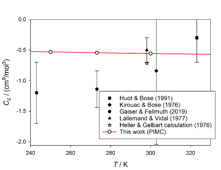
Figure 1: Comparison of calculated values of $C_{\varepsilon}(T)$ for ⁴He with those derived from experiment Huot and Bose (1991); Kirouac and Bose (1976); Gaiser and Fellmuth (2019); Lallemand and Vidal (1977) at higher temperatures. The classical calculation of Heller and GelbartHeller and Gelbart (1974) is also shown.

Figure 2 shows a comparison with data at low temperatures; note that points by White and GuganWhite and Gugan (1992) near 11 K and 18 K lie below the bottom of the plot but the tops of their large error bars are visible. Our results indicate a relatively flat temperature dependence; it remains to be seen whether this will still be true when a quantitatively accurate three-body polarizability becomes available. Figure 2 also displays the result of a classical calculation of $C_{\varepsilon}(T)$, which becomes increasingly inaccurate below 20 K.

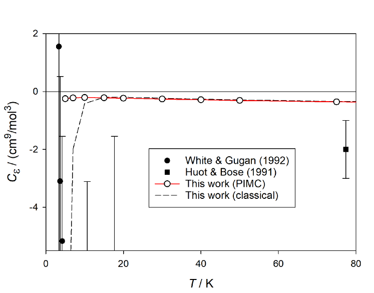
Figure 2: Comparison of calculated values of $C_{\varepsilon}(T)$ for ⁴He with those derived from experiment Huot and Bose (1991); White and Gugan (1992) at low temperatures. Two points from White and GuganWhite and Gugan (1992) are below the bottom of the plot; only the tops of their error bars are visible.

V.2 Neon

In the case of neon, we used the latest pair potential and pair polarizability by Hellmann et al. Hellmann et al. (2021) as well as the extended Axilrod–Teller three-body potential by Schwerdtfeger and Hermann. Schwerdtfeger and Hermann (2009) Dr. Hellmann provided us with the anisotropic component of the pair polarizability, which was not reported in the original paper. Hellmann (2021) (Helmut-Schmidt-Universität/Universität der Bundeswehr Hamburg)

Our calculated values are reported in Tab. 2. In this case, we did not perform the propagation of the uncertainty from the potentials and the two-body polarizability because some of these quantities do not have an uncertainty estimate, so we report only the statistical uncertainty of our calculation.

It is interesting to note that the effect of the three-body polarizability on $C_{\varepsilon}$ is quite significant. Using classical calculations as an example, the value of $C_{\varepsilon}$ obtained neglecting the three-body polarizability at $T=300$ K would be $-0.914$ cm⁹ mol^-3, a 50% difference from the value obtained including it. The effect of the approximate three-body dipole term is larger than for ⁴He but still negligible, making $C_{\varepsilon}$ less negative by an amount on the order of $0.01$ cm⁹ mol^-3 at temperatures near 300 K.

Table 2: The third dielectric virial coefficient $C_{\varepsilon}$ for ²⁰Ne and its uncertainty. The $U^{*}(C_{\varepsilon})$ are incomplete expanded uncertainties at $k=2$ and only include the statistical uncertainty of the path-integral Monte Carlo calculation. Uncertainty contributions from the two- and three-body potentials and polarizabilities and three-body dipole moment are not included; in several cases the information needed to estimate these uncertainties is not available. The last column reports the value of the third dielectric virial coefficient calculated in the classical approximation.

Temperature	$C_{\varepsilon}(T)$	$U^{*}(C_{\varepsilon})$	$C_{\varepsilon}^{\mathrm{cl}}(T)$
(K)	(cm9 mol-3)	(cm9 mol-3)	(cm9 mol-3)
$20$	$-19.997$	$0.040$	$-36.961$
$25$	$-6.167$	$0.026$	$-9.475$
$30$	$-2.836$	$0.020$	$-3.752$
$35$	$-1.756$	$0.018$	$-2.063$
$40$	$-1.332$	$0.016$	$-1.456$
$45$	$-1.182$	$0.015$	$-1.215$
$50$	$-1.117$	$0.014$	$-1.117$
$55$	$-1.088$	$0.012$	$-1.081$
$60$	$-1.075$	$0.013$	$-1.075$
$65$	$-1.097$	$0.013$	$-1.084$
$70$	$-1.113$	$0.012$	$-1.099$
$75$	$-1.123$	$0.010$	$-1.118$
$80$	$-1.158$	$0.012$	$-1.139$
$85$	$-1.174$	$0.011$	$-1.161$
$90$	$-1.188$	$0.011$	$-1.182$
$95$	$-1.223$	$0.012$	$-1.204$
$100$	$-1.236$	$0.011$	$-1.224$
$150$	$-1.409$	$0.009$	$-1.403$
$200$	$-1.540$	$0.008$	$-1.540$
$250$	$-1.647$	$0.008$	$-1.650$
$300$	$-1.744$	$0.009$	$-1.743$
$350$	$-1.824$	$0.010$	$-1.822$
$400$	$-1.890$	$0.009$	$-1.892$
$500$	$-2.004$	$0.009$	$-2.009$
$600$	$-2.105$	$0.009$	$-2.105$
$700$	$-2.183$	$0.009$	$-2.185$
$800$	$-2.254$	$0.009$	$-2.253$
$900$	$-2.312$	$0.009$	$-2.312$
$1000$	$-2.370$	$0.009$	$-2.364$
$1500$	$-2.555$	$0.009$	$-2.549$
$2000$	$-2.670$	$0.010$	$-2.662$

Figure 3 compares our calculated values with the very limited, and mutually inconsistent, experimental data available. The point from Gaiser and Fellmuth Gaiser and Fellmuth (2019) is shown with error bars corresponding to one standard uncertainty and was extracted from their dielectric-constant gas thermometry data by Rourke. Rourke (2021) Few conclusions can be drawn, especially since we do not know the accuracy of the three-body approximations, but the large negative values attained below 40 K might have consequences for gas-based metrology in that temperature range.

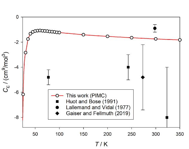
Figure 3: Comparison of calculated values of $C_{\varepsilon}(T)$ for neon with those derived from experiment. Huot and Bose (1991); Lallemand and Vidal (1977); Gaiser and Fellmuth (2019)

V.3 Argon

In the case of ⁴⁰Ar, we used the pair potential developed by Patkowski and Szalewicz, Patkowski and Szalewicz (2010) the pair polarizability by Vogel et al., Vogel et al. (2010) and the three-body potential by Cencek et al. Cencek et al. (2013) We again estimated the three-body polarizability by the superposition approximation and the three-body dipole moment with the formulation of Li and Hunt.Li and Hunt (1997) Our results are reported in Tab. 3.

Table 3: The third dielectric virial coefficient $C_{\varepsilon}$ for ⁴⁰Ar and its uncertainty. The $U^{*}(C_{\varepsilon})$ are incomplete expanded uncertainties at $k=2$ and include the statistical uncertainty of the path-integral Monte Carlo calculation and the propagated uncertainty from the potentials and the two-body polarizability. There is an unknown systematic uncertainty contribution from the superposition approximation and the approximation of the three-body dipole term. The last column reports the value of the third dielectric virial coefficient calculated in the classical approximation.

Temperature	$C_{\varepsilon}(T)$	$U^{*}(C_{\varepsilon})$	$C_{\varepsilon}^{\mathrm{cl}}(T)$
(K)	(cm9 mol-3)	(cm9 mol-3)	(cm9 mol-3)
$50$	$7315$	$641$	$7844$
$75$	$446$	$49$	$467$
$100$	$13$	$14$	$16$
$125$	$-60$	$9$	$-60$
$150$	$-78$	$8$	$-78$
$175$	$-82$	$7$	$-82$
$200$	$-82$	$7$	$-82$
$250$	$-81$	$7$	$-80$
$273.16$	$-79$	$7$	$-79$
$300$	$-78$	$7$	$-78$
$350$	$-76$	$7$	$-76$
$400$	$-75$	$7$	$-75$
$450$	$-74$	$7$	$-74$
$500$	$-73$	$7$	$-73$
$600$	$-72$	$7$	$-72$
$700$	$-72$	$7$	$-72$
$800$	$-72$	$7$	$-72$
$900$	$-71$	$7$	$-72$
$1000$	$-71$	$6$	$-72$
$1500$	$-72$	$6$	$-73$
$2000$	$-74$	$6$	$-74$

Figure 4 shows our calculated results along with experimental values for $C_{\varepsilon}$, which are somewhat more numerous than for the other two gases. The Gaiser and Fellmuth pointGaiser and Fellmuth (2019) was obtained in the same manner as described above for helium, using literature values for argon’s third density virial coefficientCencek et al. (2013) and second dielectric virial coefficient.Garberoglio and Harvey (2020a) The points shown from Achtermann and coworkersAchtermann, Magnus, and Bose (1991); Achtermann et al. (1993) are not $C_{\varepsilon}$ but instead $C_{\mathrm{R}}$, the third refractivity virial coefficient. The difference between $C_{\varepsilon}$ and $C_{\mathrm{R}}$ is expected to be small ($B_{\varepsilon}$ and $B_{\mathrm{R}}$ differ by only about 1%Garberoglio and Harvey (2020a)), so $C_{\mathrm{R}}$ still provides a valuable comparison.

Our calculated results are again reasonably consistent with the scattered experimental data. Figure 4 also shows the results that would be obtained in the absence of the three-body polarizability; it is evident that the three-body polarizability contributes a large amount to $C_{\varepsilon}$ and is necessary to obtain agreement with experimental data. In the case of argon, the contribution from the three-body dipole term is not completely negligible; it makes $C_{\varepsilon}$ less negative by an amount on the order of 1 cm⁹ mol^-3 at temperatures near 300 K.

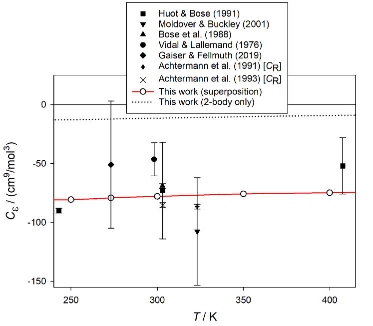
Figure 4: Comparison of calculated values of $C_{\varepsilon}(T)$ for argon with those derived from experiment. Bose et al. (1988); Huot and Bose (1991); Moldover and Buckley (2001); Gaiser and Fellmuth (2019); Vidal and Lallemand (1976); Achtermann, Magnus, and Bose (1991); Achtermann et al. (1993)

VI Conclusions

We have presented the first complete framework for calculating the third dielectric virial coefficient of gases with rigorous accounting for quantum effects, including exchange effects. Calculations of $C_{\varepsilon}(T)$ were performed for helium, neon, and argon, using the best available pair and three-body potentials and pair polarizability functions. Our calculations yielded results in qualitative agreement with the limited experimental data available.

The results presented in Sec. V are not yet suitable for rigorous metrological use, because there is an unknown systematic uncertainty due to the use of the superposition approximation for the three-body nonadditive polarizability. Because the relative contribution of the three-body polarizability to $C_{\varepsilon}$ is large, especially for argon, an error in the superposition approximation could produce a significant error in $C_{\varepsilon}(T)$. Qualitatively, since the superposition approximation produces the correct long-range behavior, we might expect it to be accurate at conditions where dispersion forces dominate the interactions (as is the case for argon at temperatures of practical interest), while perhaps losing accuracy where repulsive configurations dominate the virial coefficients (as is the case for helium at ambient temperatures). A possibly analogous situation is the third density virial coefficient of helium, where the Axilrod-Teller three-body potential, which is an induced dipole model valid at long range, produces a correction of the wrong sign above approximately 170 K.Garberoglio and Harvey (2009)

There is an additional unknown systematic uncertainty due to the lack of a three-body dipole moment surface for the gases considered. While preliminary calculations using an approximation valid in the long-range limit suggest that this effect is negligible for helium and neon, and small for argon, a quantitative estimate is needed for a rigorous uncertainty budget. If this three-body dipole contribution is truly small, the relative uncertainty of the estimate could be large without significantly increasing the total uncertainty in the calculated $C_{\varepsilon}$.

It is therefore imperative for the use of these dielectric virial coefficients in metrology that quantitative surfaces, with uncertainty estimates, be developed for the three-body polarizability (and, with less urgency, for the three-body dipole moment). Such an effort is currently underway for helium. Garberoglio et al.

Data Availability

The data that support the findings of this study are available within the article.

References

- Gaiser, Zandt, and Fellmuth (2015) C. Gaiser, T. Zandt, and B. Fellmuth, “Dielectric-constant gas thermometry,” Metrologia 52, S217–S226 (2015).
- Gaiser, Fellmuth, and Haft (2017) C. Gaiser, B. Fellmuth, and N. Haft, “Primary thermometry from 2.5 K to 140 K applying dielectric-constant gas thermometry,” Metrologia 54, 141–147 (2017).
- Gaiser et al. (2017) C. Gaiser, B. Fellmuth, N. Haft, A. Kuhn, B. Thiele-Krivoi, T. Zandt, J. Fischer, O. Jusko, and W. Sabuga, “Final determination of the Boltzmann constant by dielectric-constant gas thermometry,” Metrologia 54, 280–289 (2017).
- Gaiser, Fellmuth, and Haft (2020) C. Gaiser, B. Fellmuth, and N. Haft, “Thermodynamic-temperature data from 30 K to 200 K,” Metrologia 57, 055003 (2020).
- Gaiser, Fellmuth, and Sabuga (2020) C. Gaiser, B. Fellmuth, and W. Sabuga, “Primary gas-pressure standard from electrical measurements and thermophysical ab initio calculations.” Nature Phys. 16, 177–180 (2020).
- Piszczatowski et al. (2015) K. Piszczatowski, M. Puchalski, J. Komasa, B. Jeziorski, and K. Szalewicz, “Frequency-dependent polarizability of helium including relativistic effects with nuclear recoil terms,” Phys. Rev. Lett. 114, 173004 (2015).
- Rourke et al. (2019) P. M. C. Rourke, C. Gaiser, B. Gao, D. Madonna Ripa, M. R. Moldover, L. Pitre, and R. J. Underwood, “Refractive-index gas thermometry,” Metrologia 56, 032001 (2019).
- Gao et al. (2020) B. Gao, H. Zhang, D. Han, C. Pan, H. Chen, Y. Song, W. Liu, J. Hu, X. Kong, F. Sparasci, M. Plimmer, E. Luo, and L. Pitre, “Measurement of thermodynamic temperature between 5 K and 24.5 K with single-pressure refractive-index gas thermometry,” Metrologia 57, 065006 (2020).
- Madonna Ripa et al. (2021) D. Madonna Ripa, D. Imbraguglio, C. Gaiser, P. P. M. Steur, D. Giraudi, M. Fogliati, M. Bertinetti, G. Lopardo, R. Dematteis, and R. M. Gavioso, “Refractive index gas thermometry between 13.8 K and 161.4 K,” Metrologia 58, 025008 (2021).
- Rourke (2021) P. M. Rourke, “Perspective on the refractive-index gas metrology data landscape,” J. Phys. Chem. Ref. Data 50, 033104 (2021).
- Garberoglio and Harvey (2020a) G. Garberoglio and A. H. Harvey, “Path-integral calculation of the second dielectric and refractivity virial coefficients of helium, neon, and argon,” J. Res. Natl. Inst. Stand. Technol. 125, 125022 (2020a).
- Puchalski et al. (2020) M. Puchalski, K. Szalewicz, M. Lesiuk, and B. Jeziorski, “QED calculation of the dipole polarizability of helium atom,” Phys. Rev. A 101, 022505 (2020).
- Hirschfelder, Curtiss, and Bird (1954) J. O. Hirschfelder, C. F. Curtiss, and R. B. Bird, Molecular Theory of Gases and Liquids (John Wiley & Sons, New York, 1954).
- Song and Luo (2020) B. Song and Q.-Y. Luo, “Accurate second dielectric virial coefficient of helium, neon, and argon from ab initio potentials and polarizabilities,” Metrologia 57, 025007 (2020).
- Garberoglio and Harvey (2009) G. Garberoglio and A. H. Harvey, “First-principles calculation of the third virial coefficient of helium,” J. Res. Nat. Inst. Stand. Technol. 114, 249–262 (2009).
- Garberoglio, Moldover, and Harvey (2011) G. Garberoglio, M. R. Moldover, and A. H. Harvey, “Improved first-principles calculation of the third virial coefficient of helium,” J. Res. Nat. Inst. Stand. Technol. 116, 729–742 (2011).
- Heller and Gelbart (1974) D. F. Heller and W. M. Gelbart, “Short range electronic distortion and the density dependent dielectric function of simple gases,” Chem. Phys. Lett. 27, 359–364 (1974).
- Puchalski et al. (2016) M. Puchalski, K. Piszczatowski, J. Komasa, B. Jeziorski, and K. Szalewicz, “Theoretical determination of the polarizability dispersion and the refractive index of helium,” Phys. Rev. A 93, 032515 (2016).
- Rourke (2017) P. M. C. Rourke, “NRC microwave refractive index gas thermometry implementation between 24.5 K and 84 K,” Int. J. Thermophys. 38, 107 (2017).
- Gaiser and Fellmuth (2019) C. Gaiser and B. Fellmuth, “Highly-accurate density-virial-coefficient values for helium, neon, and argon at 0.01 °C determined by dielectric-constant gas thermometry,” J. Chem. Phys. 150, 134303 (2019).
- O’Brien et al. (1973) E. F. O’Brien, V. P. Gutschick, V. McKoy, and J. P. McTague, “Polarizability of interacting atoms: Relation to collision-induced light scattering and dielectric models,” Phys. Rev. A 8, 690–696 (1973).
- Alder et al. (1980) B. J. Alder, J. C. Beers, H. L. Strauss, and J. J. Weis, “Dielectric constant of atomic fluids with variable polarizability,” Proc. Nat. Acad. Sci. 77, 3098–3102 (1980).
- Vidal and Lallemand (1976) D. Vidal and M. Lallemand, “Evolution of the Clausius–Mossotti function of noble gases and nitrogen, at moderate and high density, near room temperature,” J. Chem. Phys. 64, 4293–4302 (1976).
- Lallemand and Vidal (1977) M. Lallemand and D. Vidal, “Variation of the polarizability of noble gases with density,” J. Chem. Phys. 66, 4776–4780 (1977).
- Hill (1958) T. L. Hill, “Theory of the dielectric constant of imperfect gases and dilute solutions,” J. Chem. Phys. 28, 61–66 (1958).
- Moszynski, Heijmen, and van der Avoird (1995) R. Moszynski, T. G. A. Heijmen, and A. van der Avoird, “Second dielectric virial coefficient of helium gas: quantum-statistical calculations from an ab initio interaction-induced polarizability,” Chem. Phys. Lett. 247, 440–446 (1995).
- Gray, Gubbins, and Joslin (2011) C. G. Gray, K. E. Gubbins, and C. G. Joslin, Theory of Molecular Fluids, Vol. 2: Applications (Oxford Science Publications, 2011).
- Jackson (1998) J. D. Jackson, Classical Electrodynamics, 3rd ed. (John Wiley & Sons, New York, 1998).
- (29) G. Garberoglio, A. H. Harvey, J. Lang, M. Lesiuk, M. Przybytek, and B. Jeziorski, To be published.
- Hill (1959) T. L. Hill, “Theory of the dielectric constant of dilute solutions. II,” J. Chem. Phys. 30, 1114 (1959).
- Martin (1974) P. H. Martin, “The long-range dipole moment of three identical atoms,” Mol. Phys. 27, 129–134 (1974).
- Bruch, Corcoran, and Weinhold (1978) L. W. Bruch, C. T. Corcoran, and F. Weinhold, “On the dipole moment of three identical spherical atoms,” Mol. Phys. 35, 1205–1210 (1978).
- Li and Hunt (1997) X. Li and K. L. C. Hunt, “Nonadditive three-body dipoles of inert gas trimers and H: Long-range effects in far infrared absorption and triple vibrational transitions,” J. Chem. Phys. 107, 4133–4153 (1997).
- Buckingham and Hands (1991) A. Buckingham and I. Hands, “The three-body contribution to the polarizability of a trimer of inert gas atoms using a dipole–induced-dipole model,” Chem. Phys. Lett. 185, 544–549 (1991).
- Gelbart (1974) W. M. Gelbart, “Depolarized light scattering by simple fluids,” in Adv. Chem. Phys., Vol. XXVI (John Wiley & Sons, Ltd, 1974) pp. 1–106.
- Champagne, Li, and Hunt (2000) M. Champagne, X. Li, and K. Hunt, “Nonadditive three-body polarizabilities of molecules interacting at long range: Theory and numerical results for the inert gases, H2, N2, CO2, and CH4,” J. Chem. Phys. 112, 1893–1906 (2000).
- Feynman and Hibbs (1965) R. P. Feynman and A. Hibbs, Quantum Mechanics and Path Integrals (McGraw-Hill, New York, 1965).
- Garberoglio and Harvey (2011) G. Garberoglio and A. H. Harvey, “Path-integral calculation of the third virial coefficient of quantum gases at low temperatures,” J. Chem. Phys. 134, 134106 (2011).
- Garberoglio and Harvey (2020b) G. Garberoglio and A. H. Harvey, “Erratum: Path-integral calculation of the third virial coefficient of quantum gases at low temperatures,” J. Chem. Phys. 152, 199903 (2020b).
- Garberoglio (2008) G. Garberoglio, “Boltzmann bias grand canonical Monte Carlo.” J. Chem. Phys. 128, 134109 (2008).
- Garberoglio, Moldover, and Harvey (2020) G. Garberoglio, M. R. Moldover, and A. H. Harvey, “Erratum: Improved first-principles calculation of the third virial coefficient of helium,” J. Res. Nat. Inst. Stand. Technol. 125, 125019 (2020).
- Garberoglio (2012) G. Garberoglio, “Quantum effects on virial coefficients: a numerical approach using centroids,” Chem. Phys. Lett. 525-526, 19 (2012).
- Kreckel (1997) R. Kreckel, “Parallelization of adaptive MC integrators,” Comp. Phys. Comm. 106, 258 (1997).
- Czachorowski et al. (2020) P. Czachorowski, M. Przybytek, M. Lesiuk, M. Puchalski, and B. Jeziorski, “Second virial coefficients for 4He and 3He from an accurate relativistic interaction potential,” Phys. Rev. A 102, 042810 (2020).
- Cencek, Patkowski, and Szalewicz (2009) W. Cencek, K. Patkowski, and K. Szalewicz, “Full-configuration-interaction calculation of three-body nonadditive contribution to helium interaction potential,” J. Chem. Phys. 131, 064105 (2009).
- Cencek, Komasa, and Szalewicz (2011) W. Cencek, J. Komasa, and K. Szalewicz, “Collision-induced dipole polarizability of helium dimer from explicitly correlated calculations,” J. Chem. Phys. 135, 014301 (2011).
- Huot and Bose (1991) J. Huot and T. K. Bose, “Experimental determination of the dielectric virial coefficients of atomic gases as a function of temperature,” J. Chem. Phys. 95, 2683–2687 (1991).
- Kirouac and Bose (1976) S. Kirouac and T. K. Bose, “Polarizability and dielectric properties of helium,” J. Chem. Phys. 64, 1580–1582 (1976).
- White and Gugan (1992) M. P. White and D. Gugan, “Direct measurements of the dielectric virial coefficients of 4He between 3 K and 18 K,” Metrologia 29, 37–57 (1992).
- Hellmann et al. (2021) R. Hellmann, C. Gaiser, B. Fellmuth, T. Vasyltsova, and E. Bich, “Thermophysical properties of low-density neon gas from highly accurate first-principles calculations and dielectric-constant gas thermometry measurements,” J. Chem. Phys. 154, 164304 (2021).
- Schwerdtfeger and Hermann (2009) P. Schwerdtfeger and A. Hermann, “Equation of state for solid neon from quantum theory,” Phys. Rev. B 80, 064106 (2009).
- Hellmann (2021) (Helmut-Schmidt-Universität/Universität der Bundeswehr Hamburg) R. Hellmann (Helmut-Schmidt-Universität/Universität der Bundeswehr Hamburg), (2021), private communication.
- Patkowski and Szalewicz (2010) K. Patkowski and K. Szalewicz, “Argon pair potential at basis set and excitation limits,” J. Chem. Phys. 133, 094304 (2010).
- Vogel et al. (2010) E. Vogel, B. Jäger, R. Hellmann, and E. Bich, “Ab initio pair potential energy curve for the argon atom pair and thermophysical properties for the dilute argon gas. II. Thermophysical properties for low-density argon,” Mol. Phys. 108, 3335–3352 (2010).
- Cencek et al. (2013) W. Cencek, G. Garberoglio, A. H. Harvey, M. O. McLinden, and K. Szalewicz, “Three-body nonadditive potential for argon with estimated uncertainties and third virial coefficient,” J. Phys. Chem. A 117, 7542–7552 (2013).
- Achtermann, Magnus, and Bose (1991) H. J. Achtermann, G. Magnus, and T. K. Bose, “Refractivity virial coefficients of gaseous , , , , , , , He, and Ar,” J. Chem. Phys. 94, 5669–5684 (1991).
- Achtermann et al. (1993) H. J. Achtermann, J. G. Hong, G. Magnus, R. A. Aziz, and M. J. Slaman, “Experimental determination of the refractivity virial coefficients of atomic gases,” J. Chem. Phys. 98, 2308–2318 (1993).
- Bose et al. (1988) T. K. Bose, K. Boudjarane, J. Huot, and J. M. St-Arnaud, “Refractivity virial coefficients of and –Ar mixtures,” J. Chem. Phys. 89, 7435–7440 (1988).
- Moldover and Buckley (2001) M. R. Moldover and T. J. Buckley, “Reference values of the dielectric constant of natural gas components determined with a cross capacitor,” Int. J. Thermophys. 22, 859–885 (2001).