Superhorizon perturbations: A possible explanation of the Hubble–Lemaître Tension and the Large Scale Anisotropy of the Universe

Abstract

Current cosmological observations point to a serious discrepancy between the observed Hubble parameter obtained using direct and cosmic microwave background radiation (CMBR) measurements. Besides this, the so called Hubble–Lemaître tension, we also find considerable evidence in diverse cosmological observables that indicate violation of the cosmological principle. In this paper, we suggest that both these discrepancies are related and can be explained by invoking superhorizon perturbations in the Universe. We implement this by considering a single superhorizon mode and showing that it leads to both a dipole in large scale structures and a shift in the Hubble–Lemaître parameter. Furthermore, the shift is found to be independent of redshift up to a certain distance. This is nicely consistent with the data.

I Introduction

Around 90 years ago, Georges Henri Joseph Édouard Lemaître proposed that an expanding universe can explain the recession of nearby galaxies [1]. With his expanding universe model, Lemaître derived the speed–distance relationship, the “Hubble’s Law”, and estimated the rate of cosmic expansion, i.e., the “Hubble constant”, equal to $645\,{\rm km\,s^{-1}\,Mpc^{-1}}$ [2, 3, 4]. He did this by combining Gustaf Strömberg’s redshift data [5] (who relied mostly on Vesto Slipher’s work [6]) and Hubble’s distances that were extracted using magnitudes [7, 3]. Soon after, Edwin Powell Hubble published his famous paper [8] where he and his assistant, Milton Humason used better stellar distance indicators such as Cepheid variables, novae and velocities. The velocity information was primarily extracted from the spectroscopic Doppler-shift observations due to Vesto Melvin Slipher [9]. This established a linear relationship between velocity & distance and determined the value for the cosmic expansion term, the Hubble’s constant, equal to $500\,{\rm km\,s^{-1}\,Mpc^{-1}}$. Hubble’s remarkable observational relationship and Hubble constant value were obtained using only 24 nearby galaxies for which both measured velocities and distances were available with certain accuracy. Shortly after Lemaître and Hubble’s discovery, cosmologists, including Einstein, became aware that far away objects are moving faster and thus the expanding universe model was established.

The theoretical and observational advances of cosmology have confirmed a dark and exotic universe that is well described by the Friedman–Lemaître –Robertson–Walker (FLRW) metric [10, 11, 12, 13, 14, 15, 16, 17], consisting of $\approx 70$% dark energy ($\Lambda$), $\approx 25$% cold dark matter (CDM), and with only $\approx 5$% of familiar baryonic matter. Presently, the standard $\Lambda$CDM cosmological model that assumes zero spatial curvature ($\Omega_{\mathrm{k}}=0$) together with isotropy and homogeneity, provides the simplest explanation of our universe. It provides a good fit to a large number of cosmological observations, such as the CMB radiation, primordial helium abundance, baryonic acoustic oscillations (BAO), galaxy clustering, Hubble parameter measurements etc.

Inspite of all these successes, there have been several different observations showing significant tension with the standard $\Lambda$CDM. In particular, the ‘direct’ measurements of the Hubble–Lemaître parameter show a clear mismatch from the ones observed using ‘indirect’ CMB measurements. Most notably, the recent direct measurement of Hubble–Lemaître parameter from Supernovae H0 for the Equation of State (SH0ES) collaboration, that uses Cepheid calibrated SNIa, yields $H_{0}=73.5\pm 1.4\,{\rm km\,s^{-1}\,Mpc^{-1}}$ [18]. To the contrary, the Planck satellite using its precise CMB radiation fluctuation measurements [19] finds $H_{0}=67.36\pm 0.54\,{\rm km\,s^{-1}\,Mpc^{-1}}$. These two disagree with each other at $4.2\sigma$ [20] and this disagreement is widely known as Hubble–Lemaître tension in the literature (see however [21] for a contrary view). For a review on the Hubble–Lemaître tension, see [22, 23, 24].

There have been several simultaneous attempts to calculate $H_{0}$ value using direct and indirect methods. On one hand, indirect methods usually employ CMB or Big Bang nucleosynthesis (BBN) with galaxy clustering measurements, viz., Sloan Digital Sky Survey (SDSS): Baryon Oscillation Spectroscopic Survey (BOSS), extended Baryon Oscillation Spectroscopic Survey (eBOSS) etc. They produce Hubble–Lemaître parameter value roughly in agreement with the aforementioned Planck satellite value [25, 26, 27]. Whereas, the direct measurements, now extending across kpc to Gpc scales, include observations from Cepheids-SNIa [28], Tip of the red-giant branch (TRGB)-SNIa [18], Miras-SNIa [29], Masers [30], Surface brightness fluctuations [31], Tully-Fisher relation [32], gravitational waves [33, 34] etc., are roughly in agreement with SH0ES observation. The direct measurements also include observations of lensing systems — for example the H0 Lenses in COSMOGRAIL’s Wellspring (H0LiCOW) collaboration [35] finds $H_{0}=73.3^{+1.7}_{-1.8}\,{\rm km\,s^{-1}\,Mpc^{-1}}$. Additionally, the Carnegie–Chicago Hubble Program, based on a calibration of TRGB applied to SNIa [36], finds somewhat lower value of Hubble–Lemaître parameter equal to $69.8\pm 1.9\,{\rm km\,s^{-1}\,Mpc^{-1}}$. Ever since Hubble–Lemaître discovery, numerous extreme precision measurements of the Hubble–Lemaître parameter have been carried out. Over the decades and to ever increasing distances, a variety of probes like SNIa standard candles [37, 38, 39, 40, 41], improved stellar/Cepheid distance indicators [42] etc., have been deployed to achieve this. These advancements have made the directly measured value of the Hubble parameter extremely accurate — from Hubble’s value of $H_{0}=500\,{\rm km\,s^{-1}\,Mpc^{-1}}$ to the present value $H_{0}=73\pm\sim 2\,{\rm km\,s^{-1}\,Mpc^{-1}}$. This has allowed us to make a close comparison between CMB derived $H_{0}$ value and the one from direct measurements.

To resolve this conflict between directly and indirectly measured $H_{0}$ values, there has been a flurry of proposals in the literature (see [22, 43] for a review of various solutions). These papers present various novel approaches such as the modification of the dark energy [44, 45, 46, 47, 48, 49, 50, 51, 52, 53], introduction of non-standard neutrino interaction terms [54, 55, 56, 57, 58, 59], introduction of the fifth force [60], emerging spatial curvature on account of the non-linear relativistic evolution [61], modification of theory of gravity [62, 63, 64, 65], the modification of the $\Lambda$CDM by modifying or adding energy components to it [66, 67, 68] etc.

In addition to the Hubble–Lemaître tension, there exist other observations which also suggest a potential departure from the $\Lambda$CDM model. Some of these challenge the basic foundations of the model — the cosmological principle. These include dipole anisotropy in radio polarization offset angles [69], alignment of CMB quadrupole and octopole [70, 71, 72], alignment of quasar polarizations [73], dipole anisotropy in radio source counts [74, 75, 76, 77, 78, 79, 80] & radio polarizations [81], bulk flow in X-ray clusters [82] etc. Remarkably, all these indicate a preferred direction close to the observed CMB dipole [83]. A recent study claims a dipole signal in quasar source counts at infrared frequencies which shows a deviation from the expected CMB dipole at $4.9\sigma$ level [84]. There also exist several claims of anisotropy in the Hubble constant [85, 86, 87, 88]. These observations suggest a potential departure from isotropy on the largest distance scales. A comprehensive discussion of such isotropy violations is given in [89].

In this letter, we suggest that the two problems, i.e. (a) Hubble–Lemaître tension and (b) the observed violation of isotropy at large distance scales are related. We propose a novel and elegant solution to both problems with a minimal modification of the $\Lambda$CDM model.

II A new proposal to relax Hubble–Lemaître tension

In the late-seventies, Grishchuk & Zel’dovich [90, 91] pointed out that long wavelength, i.e., superhorizon perturbations to the metric could be significant without contradicting the observed temperature fluctuations of CMB. Such perturbations can explain the alignment of low-multipole moments of CMB [92]. We also have constraints on amplitudes and wavelengths of superhorizon perturbations from low-multipole moments of CMB [93, 94].

To explain the implementation of superhorizon modes, we consider the conventional conformal Newtonian gauge with the scalar perturbation to the flat FLRW metric given as,

$$\mathrm{d}s^{2}=-(1+2\Psi)\mathrm{d}t^{2}+a^{2}(t)(1-2\Phi)\delta_{ij}\mathrm{d}x^{i}\mathrm{d}x^{j},$$ (1)

where $a(t)$ is the usual cosmological scale factor with $a_{0}=1$. The perturbation $\Psi$ to the temporal part of the metric corresponds to the Newtonian potential. The scalar $\Phi$ is the perturbation to the spatial curvature. In the absence of anisotropic stress, $\Psi=\Phi$. A single adiabatic superhorizon mode perturbation, providing initial conditions for $\Psi$, in its simplest form can be modeled as [95, 96, 97],

$$\Psi_{\mathrm{p}}=\alpha\sin(\kappa x_{3}+\omega),$$ (2)

where the subscript ‘p’ is an abbreviation for primordial, $\alpha$ is the superhorizon mode amplitude, $x_{3}$ is the third component of the comoving position vector, $\kappa$ being the magnitude of the wave vector $\vec{k}$ and $\omega$ is a constant phase factor. Also, we have fixed the coordinate such that the wavevector $\vec{k}=\kappa{\hat{x}}_{3}$. This kind of simple superhorizon mode has been shown to significantly affect the large-scale distribution of matter and can potentially explain [96, 97] the puzzling excess dipole signal observed in radio galaxy distribution [74, 75, 76, 77, 81, 78, 79] while simultaneously explaining the alignment of CMB quadrupole and octopole [92]. The superhorizon mode in Eq. (2) introduces a perturbation to the gravitational potential between distant galaxies and us. This effectively introduces corrections to observed redshifts of galaxies. Das et. al. [97] show that a galaxy at redshift $z$ in the presence of a superhorizon perturbation $\Psi_{\mathrm{p}}$ will be observed at redshift $z_{\mathrm{obs}}$, such that

$$1+z_{\mathrm{obs}}=(1+z)(1+z_{\rm Doppler})(1+z_{\rm grav}),$$ (3)

where $z_{\rm Doppler}$ and $z_{\rm grav}$ are respectively the redshifts due to our velocity relative to large scale structure and potential perturbations introduced by superhorizon mode. The $z_{\mathrm{obs}}$ can be expanded and the leading monopole and dipole term can be written as,

$$z_{\mathrm{obs}}=\bar{z}+\gamma\cos\theta+...,$$ (4)

Here $\theta$ is the polar angle of the spherical polar coordinate system, $\gamma\equiv\gamma(z,\alpha,\kappa,\omega)$ and is small in comparison with $\bar{z}$, the monopole term. The monopole term $\bar{z}$, given in [97], is

$$z_{\rm obs}\approx\bar{z}=z+(1+z)[g(z)-g(0)]\alpha\sin\omega,$$ (5)

where $g(z)$ represents the redshift evolution of $\Psi(z)$ such that $\Psi(z)=g(z)\Psi_{\rm p}$.

Ghosh [96] and Das et. al. [97] successfully explain excess dipole signal observed with high redshift galaxies [74, 75, 76, 77, 81, 78, 79] using superhorizon perturbations. They find that a superhorizon mode, for a range of $\alpha,\kappa$ values, can consistently explain both the CMB and NVSS observations while remaining in harmony with others, viz., the dipole anisotropy in local Hubble–Lemaître parameter measurements and local bulk flow observations. Das et al. [97] note that the phase $\omega=\pi$ conventionally maximizes the dipole signal in radio galaxies. They also provide sufficient details regarding superhorizon perturbations and their applications to galaxy clustering, Hubble–Lemaître parameter anisotropy measurements, bulk flow etc. In addition to this, they find a monopole contribution which is non-zero as long as the phase $\omega\neq\pi$. The choice $\omega=\pi$ is rather special and implies that we have a preferred position in the universe. There is no physical motivation for this and here we explore the implications of the monopole term. Remarkably, we find that the monopole term in Eq. (5) potentially solves the Hubble–Lemaître tension. We consider general values of phase $\omega$ and obtain redshift monopole term in Eq. (5). The Hubble–Lemaître law (for nearby galaxies) is written as,

$${V_{\rm obs}}=H_{0}^{\rm obs}d,$$ (6)

where $V_{\rm obs}$ is the observed radial velocity of a galaxy at the proper distance $d$ and $H^{\rm obs}_{0}$ is the observed Hubble–Lemaître parameter, corresponding to the observed redshift $z_{\mathrm{obs}}$. Thus we have (assuming ${z}_{\mathrm{obs}}\ll 1$)

$${z_{\rm obs}}=\frac{V_{\rm obs}}{c}=\frac{d}{c{(H_{0}^{\rm obs})}^{-1}}.$$ (7)

Analogously, in the equation for redshift $z$, $V_{\rm obs}$ and $H^{\rm obs}_{0}$ would respectively be replaced by $V$ and $H_{0}$. Here $H_{0}$ is the Hubble–Lemaître parameter predicted from CMB measurements.

We note that the velocity measurements are carried out using Doppler shift and thus the apparent change in $z$ results a change in velocity. This eventually leads to a change in distance-velocity relation slope, i.e., Hubble–Lemaître parameter value. Therefore, if the observed redshifts $z_{\mathrm{obs}}$ differ $z$ by 10%, the directly measured value $H^{\rm obs}_{0}$ will also differ from $H_{0}$ by the same amount. As the Hubble–Lemaître tension is all about $\sim 10$% excess in directly measured Hubble–Lemaître parameter value, we seek this change in the redshift dipole term given in Eq. (5). We find that a superhorizon mode with a range of $\alpha,\ \kappa$ and $\omega$ values can consistently explain the excess galaxy dipole and Hubble–Lemaître tension. The set of values of these parameters is consistent with CMB, local bulk flow and local redshifts anisotropy limit.

II.1 Possible values of parameters

We consider Reid et al. [18] work and produce the Hubble–Lemaître measurements considering superhorizon perturbation mode. The details of the fitting procedure are given in the Appendix. The results are shown in Figure 1. Some possible sets of values of $\alpha,\kappa$ and $\omega$, that simultaneously explain the dipole from NRAO VLA Sky Survey (NVSS) data and the Hubble–Lemaître measurements are listed in Table 1. In general, a superhorizon mode with a phase $\omega$, with a ‘reasonable’ amplitude $\alpha$ and wavelength $2\pi/\kappa$ can explain excess NVSS dipole and Hubble–Lemaître tension. Furthermore, it is also noted that for a given superhorizon mode, the apparent Hubble–Lemaître parameter roughly remains the same for a very wide range of distances. The variation of $H^{\rm obs}_{0}$ with distance is given in Figure 2. We add that superhorizon modes with CMB limits along with the NVSS dipole solution curve are consistent with local Hubble dipole and bulk flow observations [97].

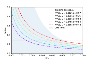
Figure 1: Plot of $|\alpha\sin\omega|$ versus $\kappa/H_{0}$ for the observed Hubble–Lemaître tension and NVSS dipole amplitude for various values of $\omega$. We have assumed dipole amplitude equal to $0.0151$ [77]. The horizontal line satisfies Reid et. al. [18] results, i.e., ${H^{\rm obs}_{0}}=73.5\,{\rm km\,s^{-1}\,Mpc^{-1}}$ at 7.57 Mpc, and the dotted dashed curves represent the NVSS excess dipole solution in $\kappa$, $\alpha$ plane with different values of phase $\omega$. The blue-shaded part denotes the region of parameter space that satisfies the CMB quadrupole constraint [95]. Note that for $\kappa$ range we have explored, and phase, $\omega\neq\pi$, only the quadrupole constraints turn out to be relevant.

Superhorizon	$\omega$	$\alpha$	$\kappa\over H_{0}$
mode
1.	$0.91\pi$	0.97	$2.581\times 10^{-3}$
2.	$0.89\pi$	0.76	$3.357\times 10^{-3}$
3.	$0.86\pi$	0.63	$4.180\times 10^{-3}$
4.	$0.84\pi$	0.54	$5.067\times 10^{-3}$
5.	$0.81\pi$	0.48	$6.037\times 10^{-3}$

Table 1: Some possible superhorizon modes $\Psi_{\mathrm{p}}$ with appropriate parameters satisfying Reid et. al. [18] results, i.e. ${H^{\rm obs}_{0}}=73.5\,{\rm km\,s^{-1}\,Mpc^{-1}}$ at 7.57 Mpc, and NVSS excess dipole simultaneously.

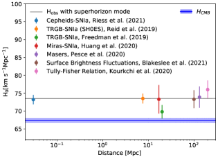
Figure 2: Apparent value of Hubble–Lemaître parameter with direct measurements at different distances. It is noted that the directly measured Hubble–Lemaître parameter remains roughly the same from distance as small as kpc to hundreds of Mpc. The Hubble–Lemaître measurements (data points) are obtained by combing many objects, the distance (x-axis) shown in figure corresponds to far most object used for analysis. All data points except CMB are direct measurements of Hubble–Lemaître parameter.

III Conclusion and Outlook

Current cosmological observations suggest two discrepancies with the $\Lambda$CDM model. These are the Hubble–Lemaître tension and the large scale anisotropy of the Universe. With more observations, these discrepancies have only grown stronger. In this paper, we have shown that both of these can be explained within the framework of a phenomenological model that assumes the existence of a superhorizon mode in the Universe. Such a mode is consistent with all existing cosmological observations and is already known to explain the CMB quadrupole-octopole alignment and the excess dipole in large scale structures. It is therefore quite fascinating that it can also explain the Hubble-Lemaitre tension, which apriori appears to be a completely independent phenomenon. The model introduces only three new parameters, namely the amplitude, wavelength and the phase of the mode. Besides this, no special fine tuning of parameters is required for fitting the observables. It leads to a Hubble parameter which is approximately constant up to distances of order few hundred Mpc, which is nicely consistent with observations. The model is likely to make a wide range of cosmological predictions which can be tested in future. In particular, it will induce a small anisotropy along with a correlated isotropic shift in several other cosmological observables, such as BAO and the epoch of reionization, besides Hubble constant. At large redshifts, the model predicts an interesting redshift dependence, which can also be tested in future studies [97], this unique feature can potentially provide a strong evidence for the existence of superhorizon modes.

Theoretically, such a superhorizon mode may arise as a stochastic phenomenon, called spontaneous breakdown of isotropy [92]. In this case it would be consistent with the cosmological principle. Another interesting possibility is that it may arise from an early phase of inflation. Inflation provides the only known theoretical explanation for the observed isotropy and homogeneity of the Universe. Since we do not so far know how the Universe originated, it is natural to assume that at early time it may be described by an unknown inhomogeneous and anisotropic metric. During inflation, and essentially independent of the initial conditions, the metric becomes almost identical to the standard FLRW metric, possibly within one $e$-fold [99]. During such an early phase, when the Universe had not yet acquired its cherished properties of isotropy and homogeneity, it can generate modes which do not obey the cosmological principle [100]. Furthermore, there exist a wide range of parameters for which these modes can affect observations today [101]. Hence these observations, which appear to show deviations from $\Lambda$CDM, might offer a glimpse into a so far obscure early phase of the Universe and may be consistent with the Big Bang paradigm [100].

Appendix A Procedure

In this Appendix we provide the details of the procedure used to fit the Hubble constant and the NVSS dipole. Using Eq. (5), we get

$$\alpha\sin\omega=\frac{\delta z/z}{(1/z+1){\Delta}g(z)},$$ (8)

where $\delta z={z}_{\mathrm{obs}}-z$ and $\Delta g(z)=g(z)-g(0)$. Further, using Eq. (7) it can be shown that $\delta z/z=\delta H_{0}/H_{0}$, with $\delta H_{0}=H^{\rm obs}_{0}-H_{0}$.

From [18, 19], we have ${H^{\rm obs}_{0}}=73.5\,{\rm km\,s^{-1}\,Mpc^{-1}}$ at $7.57$ Mpc and $H_{0}=67.36\,{\rm km\,s^{-1}\,Mpc^{-1}}$. This gives $\delta H_{0}/H_{0}=0.0911$. Following standard $\Lambda$CDM and cosmological parameters from Planck 2018 results [19], the proper distance $d=7.57$ Mpc corresponds to $z=0.0017$. So we set $\delta z/z=0.0911$ with $z=0.0017$ in Eq. (8) and obtain $\alpha\sin\omega=0.2697$. This value corresponds to the red solid line of Figure 1, satisfying Reid et. al. Hubble–Lemaître parameter observation.

In addition to the above condition, parameters $\alpha$ and $\omega$ are also constrained by CMB quadrupole and octopole values [95],

$$|\alpha_{\rm dec}\sin\omega|\leq 5.8\mathcal{Q}/(\kappa\chi_{{}_{\rm dec}})^{2},$$ (9)

$$|\alpha_{\rm dec}\cos\omega|\leq 32\mathcal{O}/(\kappa\chi_{{}_{\rm dec}})^{3},$$ (10)

where subscript ‘dec’ denotes the parameters at decoupling, $\Psi_{\rm dec}=0.937\Psi_{p}$ [95] and thus $\alpha_{\rm dec}=0.937\alpha$. $\chi_{{}_{\rm dec}}$ is the comoving distance to decoupling, $\mathcal{Q}$ and $\mathcal{O}$ are 3 times the measured rms values of the CMB quadrupole and octopole, respectively [95]. We use the latest Planck 2018 [19] values of $Q=3\sqrt{C_{2}}\leq 1.69\times 10^{-5}$ and $\mathcal{O}=3\sqrt{C_{3}}\leq 2.44\times 10^{-5}$. Following Eq. (9), we obtain the CMB limit on $|\alpha\sin\omega|$, i.e., the blue-shaded region of Figure 1. To explain Reid et al. [18] excess $H_{0}$, we impose (a) $\alpha\sin\omega=0.2697$ and (b) CMB limits. Using these, we find $\kappa/H_{0}\leq 6.29\times 10^{-3}$.

The NVSS galaxies extend over the redshift range $z=0$ to 3.5 [98, 78]. We note from Das et. al. [97] that to obtain NVSS dipole as a consequence of superhorizon mode,

$$\alpha\cos\omega=\frac{H_{0}}{\kappa}\frac{\mathcal{D}_{\rm obs}-\mathcal{B}}{\mathcal{A}_{1}(0,3.5)+\mathcal{A}_{2}(0,3.5)+\mathcal{C}(0,3.5)},$$ (11)

where $\mathcal{D}_{\rm obs}$ is the observed NVSS dipole. Other terms in Eq. (11) are defined in Das et al. [97]. To obtain $\alpha\sin\omega$ versus $\kappa/H_{0}$ curves (dashed-dotted curves in Figure 1) satisfying NVSS dipole, we multiply Eq. (11) by $\tan\omega$ after choosing a specific phase $\omega$. For the allowed $\kappa$ range, the value of $\alpha\cos\omega$ needed to explain excess NVSS dipole in Eq. (11) is much less than the octopole limit in Eq. (10).

The intersection points of red solid line and NVSS curves in Figure 1 are the possible solutions to explain both Hubble–Lemaître tension and NVSS excess dipole. The parameters for these superhorizon modes are listed in Table 1.

In Figure 2, we fix $\alpha\sin\omega$ to satisfy Reid et. al. [18] Hubble–Lemaître parameter value and then calculate $H^{\rm obs}_{0}$ predicted with superhorizon mode from data at different distances (redshifts) using Eq. (8).

References

- [1] G. Lemaître, Un Univers homogène de masse constante et de rayon croissant rendant compte de la vitesse radiale des nébuleuses extra-galactiques, Annales de la Société; Scientifique de Bruxelles 47 (1927) 49.
- [2] P. J. E. Peebles, Impact of lemaitre’s ideas on modern cosmology, in The Big Bang and Georges Lemaître, A. Berger, ed., (Dordrecht), pp. 23–30, Springer Netherlands, 1984.
- [3] M. Way and H. Nussbaumer, Lemaître’s Hubble relationship, Physics Today 64 (2011) 8 [1104.3031].
- [4] S. van den Bergh, The curious case of lemaitre’s equation no. 24, 2011.
- [5] G. Stromberg, Analysis of radial velocities of globular clusters and non-galactic nebulae., Astrophys. J. 61 (1925) 353.
- [6] V. M. Slipher, Nebulae, Proceedings of the American Philosophical Society 56 (1917) 403.
- [7] E. P. Hubble, Extragalactic nebulae., Astrophys. J. 64 (1926) 321.
- [8] E. Hubble, A relation between distance and radial velocity among extra-galactic nebulae, Proceedings of the National Academy of Sciences 15 (1929) 168 [https://www.pnas.org/content/15/3/168.full.pdf].
- [9] V. M. Slipher, Radial velocity observations of spiral nebulae, The Observatory 40 (1917) 304.
- [10] A. Friedmann, Über die Krümmung des Raumes, Zeitschrift fur Physik 10 (1922) 377.
- [11] A. Friedmann, Über die Möglichkeit einer Welt mit konstanter negativer Krümmung des Raumes, Zeitschrift fur Physik 21 (1924) 326.
- [12] G. Lemaître, Expansion of the universe, A homogeneous universe of constant mass and increasing radius accounting for the radial velocity of extra-galactic nebulae, Mon. Not. R. Astron. Soc. 91 (1931) 483.
- [13] G. Lemaître, L’Univers en expansion, Annales de la Société; Scientifique de Bruxelles 53 (1933) 51.
- [14] H. P. Robertson, Kinematics and World-Structure, Astrophys. J. 82 (1935) 284.
- [15] H. P. Robertson, Kinematics and World-Structure II., Astrophys. J. 83 (1936) 187.
- [16] H. P. Robertson, Kinematics and World-Structure III., Astrophys. J. 83 (1936) 257.
- [17] A. G. Walker, On Milne’s Theory of World-Structure, Proceedings of the London Mathematical Society 42 (1937) 90.
- [18] M. J. Reid, D. W. Pesce and A. G. Riess, An Improved Distance to NGC 4258 and Its Implications for the Hubble Constant, Astrophys. J. Lett. 886 (2019) L27 [1908.05625].
- [19] Planck Collaboration, N. Aghanim, Y. Akrami, M. Ashdown, J. Aumont, C. Baccigalupi et al., Planck 2018 results. VI. Cosmological parameters, Astron. Astrophys. 641 (2020) A6 [1807.06209].
- [20] L. A. Anchordoqui and S. E. Perez Bergliaffa, Hot thermal universe endowed with massive dark vector fields and the Hubble tension, Phys. Rev. D 100 (2019) 123525 [1910.05860].
- [21] M. Rameez and S. Sarkar, Is there really a Hubble tension?, Class. Quant. Grav. 38 (2021) 154005 [1911.06456].
- [22] E. Di Valentino, O. Mena, S. Pan, L. Visinelli, W. Yang, A. Melchiorri et al., In the realm of the Hubble tension-a review of solutions, Classical and Quantum Gravity 38 (2021) 153001 [2103.01183].
- [23] G. Efstathiou, A Lockdown Perspective on the Hubble Tension (with comments from the SH0ES team), 2007.10716.
- [24] E. Di Valentino et al., Snowmass2021 - Letter of interest cosmology intertwined II: The hubble constant tension, Astropart. Phys. 131 (2021) 102605 [2008.11284].
- [25] L. Pogosian, G.-B. Zhao and K. Jedamzik, Recombination-independent Determination of the Sound Horizon and the Hubble Constant from BAO, Astrophys. J. Lett. 904 (2020) L17 [2009.08455].
- [26] S. Aiola, E. Calabrese, L. Maurin, S. Naess, B. L. Schmitt, M. H. Abitbol et al., The Atacama Cosmology Telescope: DR4 maps and cosmological parameters, J. Cosmol. Astropart. Phys. 2020 (2020) 047 [2007.07288].
- [27] S. Alam, M. Aubert, S. Avila, C. Balland, J. E. Bautista, M. A. Bershady et al., Completed SDSS-IV extended Baryon Oscillation Spectroscopic Survey: Cosmological implications from two decades of spectroscopic surveys at the Apache Point Observatory, Physical Review D. 103 (2021) 083533 [2007.08991].
- [28] A. G. Riess, S. Casertano, W. Yuan, J. B. Bowers, L. Macri, J. C. Zinn et al., Cosmic Distances Calibrated to 1% Precision with Gaia EDR3 Parallaxes and Hubble Space Telescope Photometry of 75 Milky Way Cepheids Confirm Tension with CDM, Astrophys. J. Lett. 908 (2021) L6 [2012.08534].
- [29] C. D. Huang, A. G. Riess, W. Yuan, L. M. Macri, N. L. Zakamska, S. Casertano et al., Hubble Space Telescope Observations of Mira Variables in the SN Ia Host NGC 1559: An Alternative Candle to Measure the Hubble Constant, Astrophys. J. 889 (2020) 5 [1908.10883].
- [30] D. W. Pesce, J. A. Braatz, M. J. Reid, A. G. Riess, D. Scolnic, J. J. Condon et al., The Megamaser Cosmology Project. XIII. Combined Hubble Constant Constraints, Astrophys. J. Lett. 891 (2020) L1 [2001.09213].
- [31] J. P. Blakeslee, J. B. Jensen, C.-P. Ma, P. A. Milne and J. E. Greene, The Hubble Constant from Infrared Surface Brightness Fluctuation Distances, Astrophys. J. 911 (2021) 65 [2101.02221].
- [32] E. Kourkchi, R. B. Tully, G. S. Anand, H. M. Courtois, A. Dupuy, J. D. Neill et al., Cosmicflows-4: The Calibration of Optical and Infrared Tully-Fisher Relations, Astrophys. J. 896 (2020) 3 [2004.14499].
- [33] V. Gayathri, J. Healy, J. Lange, B. O’Brien, M. Szczepanczyk, I. Bartos et al., Hubble Constant Measurement with GW190521 as an Eccentric Black Hole Merger, arXiv e-prints (2020) arXiv:2009.14247 [2009.14247].
- [34] S. Mukherjee, A. Ghosh, M. J. Graham, C. Karathanasis, M. M. Kasliwal, I. Magaña Hernandez et al., First measurement of the Hubble parameter from bright binary black hole GW190521, arXiv e-prints (2020) arXiv:2009.14199 [2009.14199].
- [35] K. C. Wong, S. H. Suyu, G. C. F. Chen, C. E. Rusu, M. Millon, D. Sluse et al., H0LiCOW – XIII. A 2.4 per cent measurement of H0 from lensed quasars: 5.3 tension between early- and late-Universe probes, Mon. Not. R. Astron. Soc. 498 (2020) 1420 [1907.04869].
- [36] W. L. Freedman, B. F. Madore, D. Hatt, T. J. Hoyt, I. S. Jang, R. L. Beaton et al., The Carnegie-Chicago Hubble Program. VIII. An Independent Determination of the Hubble Constant Based on the Tip of the Red Giant Branch, Astrophys. J. 882 (2019) 34 [1907.05922].
- [37] Supernova Search Team collaboration, Observational evidence from supernovae for an accelerating universe and a cosmological constant, Astron. J. 116 (1998) 1009 [astro-ph/9805201].
- [38] Supernova Search Team collaboration, The High Z supernova search: Measuring cosmic deceleration and global curvature of the universe using type Ia supernovae, Astrophys. J. 507 (1998) 46 [astro-ph/9805200].
- [39] S. Perlmutter, G. Aldering, G. Goldhaber, R. A. Knop, P. Nugent, P. G. Castro et al., Measurements of and from 42 High-Redshift Supernovae, Astrophys. J. 517 (1999) 565 [astro-ph/9812133].
- [40] R. P. Kirshner, Hubble’s diagram and cosmic expansion, Proceedings of the National Academy of Sciences 101 (2004) 8 [https://www.pnas.org/content/101/1/8.full.pdf].
- [41] M. Betoule, R. Kessler, J. Guy, J. Mosher, D. Hardin, R. Biswas et al., Improved cosmological constraints from a joint analysis of the SDSS-II and SNLS supernova samples, Astron. Astrophys. 568 (2014) A22 [1401.4064].
- [42] W. L. Freedman, B. F. Madore, B. K. Gibson, L. Ferrarese, D. D. Kelson, S. Sakai et al., Final results from theHubble space TelescopeKey project to measure the hubble constant, The Astrophysical Journal 553 (2001) 47.
- [43] N. Schöneberg, G. Franco Abellán, A. Pérez Sánchez, S. J. Witte, V. Poulin and J. Lesgourgues, The Olympics: A fair ranking of proposed models, 2107.10291.
- [44] G. S. Bisnovatyi-Kogan, Phenomenological model explaining Hubble Tension origin, 2002.05602.
- [45] G. Ye and Y.-S. Piao, Is the Hubble tension a hint of AdS phase around recombination?, Phys. Rev. D 101 (2020) 083507 [2001.02451].
- [46] G. Choi, M. Suzuki and T. T. Yanagida, Quintessence axion dark energy and a solution to the hubble tension, Phys. Lett. B 805 (2020) 135408 [1910.00459].
- [47] S. Panpanich, P. Burikham, S. Ponglertsakul and L. Tannukij, Resolving Hubble Tension with Quintom Dark Energy Model, Chin. Phys. C 45 (2021) 015108 [1908.03324].
- [48] T. Karwal and M. Kamionkowski, Dark energy at early times, the Hubble parameter, and the string axiverse, Phys. Rev. D 94 (2016) 103523 [1608.01309].
- [49] V. Poulin, T. L. Smith, T. Karwal and M. Kamionkowski, Early Dark Energy Can Resolve The Hubble Tension, Phys. Rev. Lett. 122 (2019) 221301 [1811.04083].
- [50] K. V. Berghaus and T. Karwal, Thermal Friction as a Solution to the Hubble Tension, Phys. Rev. D 101 (2020) 083537 [1911.06281].
- [51] J. Sakstein and M. Trodden, Early Dark Energy from Massive Neutrinos as a Natural Resolution of the Hubble Tension, Phys. Rev. Lett. 124 (2020) 161301 [1911.11760].
- [52] T. L. Smith, V. Poulin and M. A. Amin, Oscillating scalar fields and the Hubble tension: a resolution with novel signatures, Phys. Rev. D 101 (2020) 063523 [1908.06995].
- [53] S. Alexander and E. McDonough, Axion-Dilaton Destabilization and the Hubble Tension, Phys. Lett. B 797 (2019) 134830 [1904.08912].
- [54] N. Blinov, K. J. Kelly, G. Z. Krnjaic and S. D. McDermott, Constraining the Self-Interacting Neutrino Interpretation of the Hubble Tension, Phys. Rev. Lett. 123 (2019) 191102 [1905.02727].
- [55] C. D. Kreisch, F.-Y. Cyr-Racine and O. Doré, Neutrino puzzle: Anomalies, interactions, and cosmological tensions, Phys. Rev. D 101 (2020) 123505 [1902.00534].
- [56] S. Ghosh, R. Khatri and T. S. Roy, Can dark neutrino interactions phase out the Hubble tension?, Phys. Rev. D 102 (2020) 123544 [1908.09843].
- [57] H.-J. He, Y.-Z. Ma and J. Zheng, Resolving Hubble Tension by Self-Interacting Neutrinos with Dirac Seesaw, JCAP 11 (2020) 003 [2003.12057].
- [58] M. Escudero and S. J. Witte, A CMB search for the neutrino mass mechanism and its relation to the Hubble tension, Eur. Phys. J. C 80 (2020) 294 [1909.04044].
- [59] M. Escudero Abenza and S. J. Witte, Could the Hubble Tension be Pointing Towards the Neutrino Mass Mechanism?, in Prospects in Neutrino Physics, 4, 2020, 2004.01470.
- [60] H. Desmond, B. Jain and J. Sakstein, Local resolution of the Hubble tension: The impact of screened fifth forces on the cosmic distance ladder, Phys. Rev. D 100 (2019) 043537 [1907.03778].
- [61] K. Bolejko, Emerging spatial curvature can resolve the tension between high-redshift CMB and low-redshift distance ladder measurements of the Hubble constant, Phys. Rev. D 97 (2018) 103529 [1712.02967].
- [62] R. G. Vishwakarma, Resolving Hubble tension with the Milne model, Int. J. Mod. Phys. D 29 (2020) 2043025 [2011.12146].
- [63] T. Abadi and E. D. Kovetz, Can conformally coupled modified gravity solve the Hubble tension?, Phys. Rev. D 103 (2021) 023530 [2011.13853].
- [64] M. Shimon, Possible Resolution of the Hubble Tension with Weyl Invariant Gravity, 2012.10879.
- [65] V. G. Gurzadyan and A. Stepanian, Hubble tension vs two flows, Eur. Phys. J. Plus 136 (2021) 235 [2102.10100].
- [66] E. Mörtsell and S. Dhawan, Does the Hubble constant tension call for new physics?, JCAP 09 (2018) 025 [1801.07260].
- [67] M.-X. Lin, G. Benevento, W. Hu and M. Raveri, Acoustic Dark Energy: Potential Conversion of the Hubble Tension, Phys. Rev. D 100 (2019) 063542 [1905.12618].
- [68] A. Kaya, Vacuum Arbitrariness and the Hubble Tension, Phys. Rev. D 101 (2020) 083523 [2004.01199].
- [69] P. Jain and J. P. Ralston, Anisotropy in the propagation of radio polarizations from cosmologically distant galaxies, Mod. Phys. Lett. A 14 (1999) 417 [astro-ph/9803164].
- [70] A. de Oliveira-Costa, M. Tegmark, M. Zaldarriaga and A. Hamilton, The Significance of the largest scale CMB fluctuations in WMAP, Phys. Rev. D 69 (2004) 063516 [astro-ph/0307282].
- [71] C. J. Copi, D. Huterer, D. J. Schwarz and G. D. Starkman, Large-scale alignments from WMAP and Planck, Mon. Not. Roy. Astron. Soc. 449 (2015) 3458 [1311.4562].
- [72] P. K. Aluri, J. P. Ralston and A. Weltman, Alignments of parity even/odd-only multipoles in CMB, Mon. Not. Roy. Astron. Soc. 472 (2017) 2410 [1703.07070].
- [73] D. Hutsemékers, Evidence for very large-scale coherent orientations of quasar polarization vectors, A&A 332 (1998) 410.
- [74] A. K. Singal, Large Peculiar Motion of the Solar System from the Dipole Anisotropy in Sky Brightness due to Distant Radio Sources, ApJL 742 (2011) L23 [1110.6260].
- [75] C. Gibelyou and D. Huterer, Dipoles in the Sky, MNRAS 427 (2012) 1994 [1205.6476].
- [76] M. Rubart and D. J. Schwarz, Cosmic radio dipole from nvss and wenss, A&A 555 (2013) [1301.5559].
- [77] P. Tiwari, R. Kothari, A. Naskar, S. Nadkarni-Ghosh and P. Jain, Dipole anisotropy in sky brightness and source count distribution in radio NVSS data, Astroparticle Physics 61 (2015) 1 [1307.1947].
- [78] P. Tiwari and A. Nusser, Revisiting the nvss number count dipole, Journal of Cosmology and Astroparticle Physics 2016 (2016) 062 [1509.02532].
- [79] J. Colin, R. Mohayaee, M. Rameez and S. Sarkar, High redshift radio galaxies and divergence from the CMB dipole, Mon. Not. Roy. Astron. Soc. 471 (2017) 1045 [1703.09376].
- [80] C. A. P. Bengaly, R. Maartens and M. G. Santos, Probing the Cosmological Principle in the counts of radio galaxies at different frequencies, JCAP 04 (2018) 031 [1710.08804].
- [81] P. Tiwari and P. Jain, Dipole anisotropy in integrated linearly polarized flux density in NVSS data, Mon. Not. R. Astron. Soc. 447 (2015) 2658 [1308.3970].
- [82] A. Kashlinsky, F. Atrio-Barandela, H. Ebeling, A. Edge and D. Kocevski, A New Measurement of the Bulk Flow of X-Ray Luminous Clusters of Galaxies, Astrophys. J. Lett. 712 (2010) L81 [0910.4958].
- [83] J. P. Ralston and P. Jain, The Virgo alignment puzzle in propagation of radiation on cosmological scales, IJMPD 13 (2004) 1857 [astro-ph/0311430].
- [84] N. J. Secrest, S. v. Hausegger, R. Rameez, Mohamed a nd Mohayaee, S. Sarkar and J. Colin, A test of the cosmological principle with quasars, The Astrophysical Journal 908 (2021) L51.
- [85] D. L. Wiltshire, P. R. Smale, T. Mattsson and R. Watkins, Hubble flow variance and the cosmic rest frame, Physical Review D 88 (2013) .
- [86] K. Migkas, F. Pacaud, G. Schellenberger, J. Erler, N. T. Nguyen-Dang, T. H. Reiprich et al., Cosmological implications of the anisotropy of ten galaxy cluster scaling relations, Astron. Astrophys. 649 (2021) A151 [2103.13904].
- [87] P. Biermann, On the radio continuum flux from the disks of spiral galaxies, Astron. Astrophys. 53 (1976) 295.
- [88] O. Luongo, M. Muccino, E. O. Colgáin, M. M. Sheikh-Jabbari and L. Yin, On Larger Values in the CMB Dipole Direction, 2108.13228.
- [89] L. Perivolaropoulos and F. Skara, Challenges for CDM: An update, 2105.05208.
- [90] L. P. Grishchuk and I. B. Zeldovich, Long-wavelength perturbations of a Friedmann universe, and anisotropy of the microwave background radiation, Astron. Zh. 55 (1978) 209.
- [91] L. P. Grishchuk and I. B. Zeldovich, Long-wavelength perturbations of a Friedmann universe, and anisotropy of the microwave background radiation, Sov. Astron. 22 (1978) 125.
- [92] C. Gordon, W. Hu, D. Huterer and T. M. Crawford, Spontaneous isotropy breaking: a mechanism for cmb multipole alignments, Phys. Rev. D 72 (2005) 103002 [astro-ph/0509301].
- [93] G. F. Smoot, C. L. Bennett, A. Kogut, J. Aymon, C. Backus, G. de Amici et al., Preliminary Results from the COBE Differential Microwave Radiometers: Large Angular Scale Isotropy of the Cosmic Microwave Background, Astrophys. J. Lett. 371 (1991) L1.
- [94] G. Hinshaw, D. N. Spergel, L. Verde, R. S. Hill, S. S. Meyer, C. Barnes et al., First-Year Wilkinson Microwave Anisotropy Probe (WMAP) Observations: The Angular Power Spectrum, Astrophys. J. Suppl. 148 (2003) 135 [astro-ph/0302217].
- [95] A. L. Erickcek, S. M. Carroll and M. Kamionkowski, Superhorizon perturbations and the cosmic microwave background, Physical Review D. 78 (2008) 083012 [0808.1570].
- [96] S. Ghosh, Generating intrinsic dipole anisotropy in the large scale structures, Physical Review D. 89 (2014) 063518 [1309.6547].
- [97] K. K. Das, K. Sankharva and P. Jain, Explaining excess dipole in NVSS data using superhorizon perturbation, J. Cosmol. Astropart. Phys. 2021 (2021) 035 [2101.11016].
- [98] A. Nusser and P. Tiwari, The Clustering of Radio Galaxies: Biasing and Evolution Versus Stellar Mass, ApJ 812 (2015) 85 [1505.06817].
- [99] R. M. Wald, , PhRvD 28 (1983) 2118R.
- [100] P. Rath, T. Mudholkar, P. Jain, P. Aluri and S. Panda, Direction dependence of the power spectrum and its effect on the cosmic microwave background radiation, Journal of Cosmology and Astroparticle Physics 4 (2013) 7 [1302.2706].
- [101] P. K. Aluri and P. Jain, Large Scale Anisotropy due to Pre-Inflationary Phase of Cosmic Evolution, Modern Physics Letters A 27 (2012) 50014 [1108.3643].