Recurrent Neural Network Training with Convex Loss and Regularization Functions by Extended Kalman Filtering

Abstract

This paper investigates the use of extended Kalman filtering to train recurrent neural networks with rather general convex loss functions and regularization terms on the network parameters, including $\ell_{1}$-regularization. We show that the learning method is competitive with respect to stochastic gradient descent in a nonlinear system identification benchmark and in training a linear system with binary outputs. We also explore the use of the algorithm in data-driven nonlinear model predictive control and its relation with disturbance models for offset-free closed-loop tracking.

akefnmark

Keywords: Recurrent neural networks, nonlinear system identification, extended Kalman filtering, nonlinear model predictive control.

1 Introduction

The use of artificial neural networks (NNs) for control-oriented modeling of dynamical systems, already popular in the nineties [1], is flourishing again thanks to the wide success of machine learning in many application domains and to the availability of excellent software libraries for training NN models. Most frequently, feedforward NNs are used for modeling the output function in a neural-network autoregressive model with exogenous inputs (NNARX). On the other hand, recurrent neural networks (RNNs), as they are state-space models, are often more adequate for capturing the behavior of dynamical systems in a compact way. However, contrarily to training NNARX models based on minimizing the one-step-ahead output prediction error, training RNNs is more difficult due to the presence of the hidden states of the network. To circumvent this issue, procedures for learning neural state-space models were proposed in [2, 3], based on the idea of finding a (reduced-order) state-space realization of a NNARX model during training and considering the values of a (thin) inner layer of the model as the state vector.

To avoid unrolling the open-loop prediction of an RNN over the entire training dataset, suboptimal approaches were proposed, such as truncated backpropagation through time (truncated BPTT) [4]. Motivated by the fact that a similar issue of recurrence occurs in minimizing the simulation error when training NNARX models, the authors in [5] proposed to learn RNNs based on splitting the dataset into smaller batches and penalizing the inconsistency between state predictions across consecutive batches. Due to the difficulty of computing gradients of full unrolls and/or the presence of a large number of optimization variables, these approaches are used for offline learning and rely on (batch, mini-batch, or stochastic) gradient descent methods that, although often proved to converge only for convex problems, are widely adopted with success.

To circumvent their very slow convergence and, at the same time, be able to learn NN models incrementally when new data become available, training methods based on extended Kalman filtering (EKF) have been explored in [6] for feedforward networks, treating the weight/bias terms of the network as constant states to estimate. When dealing with recurrent networks, the authors in [7] distinguish between parallel-EKF, which estimates both the hidden states and the weights/bias terms, and parameter-based EKF, that only estimates the network parameters, and focus on the latter approach, whose convergence properties were investigated in [8].

Parallel-EKF was also studied in [9] for coinciding output and state vectors, which is therefore measurable as for NNARX models. In the context of nonlinear filtering, the authors in [10] investigated a parallel-EKF approach for the special case of RNNs that are linear in the input and the output. The method was extended in [11] to make the EKF implementation more efficient by taking into account how much each network parameter affects the predicted output. An ensemble Kalman filter method was proposed in [12]. An important aspect of EKF-based learning methods is that, as remarked in [13], the filter approximately provides the minimum variance estimate of the model parameters, and hence a quantification of model uncertainty via the covariance matrix associated with the state estimation error. All the aforementioned EKF-based methods consider quadratic penalties on the output prediction errors and the weight/bias terms of the RNN.

In this paper, we also consider a parallel-EKF approach to recursively learn a general class of RNNs whose state-update and output functions are described by neural networks, including long-short term memory (LSTM) models [14], under arbitrary convex and twice-differentiable loss functions for penalizing output open-loop prediction errors and for regularizing the weight/bias terms of the RNN, and also extend to the case of $\ell_{1}$-regularization for network topology selection. We also compare EKF to different formulations based on stochastic gradient descent (SGD) methods, in which only the initial state or also the intermediate states of the RNN are treated as optimization variables. We show the superiority of EKF with respect to SGD in a nonlinear identification benchmark, and apply the method in identifying a linear dynamical system with binary outputs. We also explore the use of EKF-based learning for data-driven nonlinear MPC design, showing a relation between the use of constant disturbance models and the adaptation of the bias terms in the neural networks for offset-free tracking, which we illustrate in a nonlinear control benchmark problem.

1.1 Notation

Given a vector $v\in\mathbb{R}^{n}$ and a matrix $A\in\mathbb{R}^{m\times n}$, $v_{i}$ denotes the $i$th real-valued component of $v$, $A_{i,:}$ the $i$th row of $A$, $A_{:,j}$ its $j$th column, $A_{ij}$ its $(i,j)$th entry. Given $v\in\mathbb{R}^{n}$ and a symmetric positive semidefinite matrix $Q=Q^{\prime}\succeq 0$, $Q\in\mathbb{R}^{n\times n}$, we denote by $\|v\|_{Q}^{2}$ the quadratic form $v^{\prime}Qv$, by $\|v\|_{1}=\sum_{i=1}^{n}|v_{i}|$ the 1-norm of $v$, and by $\mathop{\rm sign}\nolimits(v)$ the vector whose $i$th component is the sign of $v_{i}$. Given $a,b\in\mathbb{N}$, $\delta_{a,b}$ denotes the Kronecker delta function ($\delta_{a,b}=1$ if $a=b$ or $0$ otherwise).

2 Recurrent neural network model

We consider recurrent neural network (RNN) models with input $u\in\mathbb{R}^{n_{u}}$, predicted output $\hat{y}\in\mathbb{R}^{n_{y}}$, and state vector $x\in\mathbb{R}^{n_{x}}$ whose state-update and output equations are described by the following parametric model

$$\begin{array}[]{rcl}x(k+1)&=&f_{x}(x(k),u(k),{\theta_{x}})\\ \hat{y}(k)&=&f_{y}(x(k),u(k),{\theta_{y}})\end{array}$$ (1)

where ${\theta_{x}}\in\mathbb{R}^{n_{\theta_{x}}}$ and ${\theta_{y}}\in\mathbb{R}^{n_{\theta_{y}}}$ collect the parameters to learn from data. Special cases of (1) are recurrent (deep) neural networks (RNNs)

$$\left\{\begin{array}[]{rcl}v_{1}^{x}(k)&=&A_{1}^{x}\left[\begin{smallmatrix}x(k)\\ u(k)\end{smallmatrix}\right]+b_{1}^{x}\\ v_{2}^{x}(k)&=&A_{2}^{x}f_{1}^{x}(v_{1}^{x}(k))+b_{2}^{x}\\ \vdots&&\vdots\\ v_{L_{x}}^{x}(k)&=&A_{L_{x}}f_{L_{x}-1}^{x}(v_{L_{x}-1}^{x}(k))+b_{L_{x}}^{x}\\ x(k+1)&=&v_{L_{x}}^{x}(k)\end{array}\right.$$ (2a)

$$\left\{\begin{array}[]{rcl}v_{1}^{y}(k)&=&A_{1}^{y}\left[\begin{smallmatrix}x(k)\\ u(k)\end{smallmatrix}\right]+b_{1}^{y}\\ v_{2}^{y}(k)&=&A_{2}^{y}f_{1}^{y}(v_{1}^{y}(k))+b_{2}^{y}\\ \vdots&&\vdots\\ v_{L_{y}}^{y}(k)&=&A_{L_{y}}^{y}f_{L_{y}-1}^{y}(v_{L_{y}-1}^{y}(k))+b_{L_{y}}^{y}\\ \hat{y}(k)&=&f_{L_{y}}^{y}(v_{L_{y}}^{y}(k))\end{array}\right.$$ (2b)

where $L_{x}-1\geq 0$ and $L_{y}-1\geq 0$ are the number of hidden layers of the state-update and output functions, respectively, $v_{i}^{x}\in\mathbb{R}^{n_{i}^{x}}$, $i=1,\ldots L_{x}-1$, $v_{L_{x}}^{x}\in\mathbb{R}^{n_{x}}$, and $v_{i}^{y}\in\mathbb{R}^{n_{i}^{y}}$, $i=1,\ldots L_{y}$, the values of the corresponding inner layers, $f_{i}^{x}:\mathbb{R}^{n_{i}^{x}}\to\mathbb{R}^{n_{i+1}^{x}}$, $i=1,\ldots L_{x}-1$, $f_{i}^{y}:\mathbb{R}^{n_{i}^{y}}\to\mathbb{R}^{n_{i+1}^{y}}$, $i=1,\ldots L_{y}-1$ the corresponding activation functions, and $f_{L_{y}}^{y}:\mathbb{R}^{n_{L_{y}}^{y}}\to\mathbb{R}^{n_{y}}$ the output function, e.g., $f_{L_{y}}^{y}(v_{L_{y}}^{y})=v_{L_{y}}^{y}$ to model numerical outputs or $[f_{L_{y}}^{y}(v_{L_{y}}^{y})]_{i}=\left(1+e^{[v_{L_{y}}^{y}]_{i}}\right)^{-1}$, $i=1,\ldots,n_{y}$, for binary outputs. The strict causality of the RNN (2b) can be simply imposed by zeroing the last $n_{u}$ columns of $A_{1}^{y}$.

The hyperparameters describing the RNN (2b) are $n_{x}$, $\{n_{i}^{x}\}$, $\{n_{y}^{y}\}$, $\{f_{i}^{x}\}$, $\{f_{i}^{y}\}$ and dictate the chosen model structure. The parameters to learn are $A_{1}^{x}$, $\ldots$, $A_{L_{x}-1}^{x}$, $b_{1}^{x}$, $\ldots$, $b_{L_{x}-1}^{x}$, $A_{1}^{y}$, $\ldots$, $A_{L_{y}-1}^{y}$, $b_{1}^{y}$, $\ldots$, $b_{L_{y}-1}^{y}$, where $A_{i}^{x}\in\mathbb{R}^{n_{i}^{x}\times n_{i-1}^{x}}$ is the matrix of weights for layer $\#i$ of the state-update neural function, $b_{i}^{x}\in\mathbb{R}^{n_{i}^{x}}$ the corresponding vector of bias terms, and $n_{0}^{x}\triangleq n_{x}+n_{u}$, $n_{L}^{x}\triangleq n_{x}$, and $A_{i}^{y}\in\mathbb{R}^{n_{i}^{y}\times n_{i-1}^{y}}$ is the matrix of weights for layer $\#i$ of the output neural function, $b_{i}^{x}\in\mathbb{R}^{n_{i}^{x}}$ the corresponding vector of bias terms, and $n_{0}^{y}\triangleq n_{x}+n_{u}$. In this case, ${\theta_{x}}$ and ${\theta_{y}}$ are the vectors obtained by stacking all the entries of the weight/bias parameters defining the state and output equations, respectively, with $n_{\theta_{x}}=\sum_{i=1}^{L_{x}}n_{i}^{x}(n_{i-1}^{x}+1)$ and $n_{\theta_{y}}=\sum_{i=1}^{L_{y}}n_{i}^{y}(n_{i-1}^{y}+1)$.

We remark that all the results reported in this paper also apply to feedforward neural networks, a special case of (2b) for $n_{x}=0$. Moreover, they can be clearly applied also to identify linear models, that is another special case of (2b) when $L_{x}=L_{y}=1$, $b_{1}^{x}=0$, $b_{1}^{y}=0$, as previously shown in [15]. Another popular instance of model (1) is the single-layer LSTM model [14]. We will consider the form proposed in [16] with output equation as in (2b).

3 RNN training problem

Consider the following RNN learning problem: Given a training dataset $D_{N}\triangleq\{u(0),y(0),\ldots,u(N-1),y(N-1)\}$, determine an optimal solution $(x_{0}^{*},\theta^{*})$ solving the following mathematical program

$$\begin{array}[]{rl}\stackbin[x_{0},\theta]{}{\min}&V(x_{0},\theta)\triangleq\displaystyle{r_{\theta}(\theta)+r_{x}(x_{0})+\frac{1}{N}\sum_{k=0}^{N-1}\ell(y(k),\hat{y}(k))}\\ \mathop{\rm s.t.}\nolimits&\mbox{model equations~{}\eqref{eq:generic-RNN} with $x(0)=x_{0}$}\end{array}$$ (3)

where $\theta\triangleq\left[\begin{smallmatrix}{\theta_{x}}\\ {\theta_{y}}\end{smallmatrix}\right]$, $\ell:\mathbb{R}^{n_{y}}\times\mathbb{R}^{n_{y}}\to\mathbb{R}$ is a loss function penalizing the dissimilarity between the training samples $y(k)$ and the predicted values $\hat{y}(k)$ generated by simulating (2b), and $r_{\theta}:\mathbb{R}^{n_{\theta}}\to\mathbb{R}$, $r_{x}:\mathbb{R}^{n_{x}}\to\mathbb{R}$ are regularization functions. In the examples reported in Section 6 we will consider the (weighted) mean-square error (MSE) loss $\ell_{\rm MSE}(y,\hat{y})=\frac{1}{2}\|y-\hat{y}\|_{W_{y}}^{2}$ where $W_{y}=W_{y}^{\prime}\succ 0$ is a weight matrix, the (modified) cross-entropy loss $\ell_{\rm CE\epsilon}(y(k),\hat{y})=\sum_{i=1}^{n_{y}}-y_{i}(k)\log(\epsilon+\hat{y}_{i})-(1-y_{i}(k))\log(1+\epsilon-\hat{y}_{i})$ for binary outputs, the Tikhonov (or $\ell_{2}$) regularization terms $r_{\theta}(\theta)=\frac{\rho_{\theta}}{2}\|\theta\|_{2}^{2}$, $r_{x}(x_{0})=\frac{\rho_{x}}{2}\|x_{0}\|_{2}^{2}$ with $\rho_{\theta},\rho_{x}\geq 0$, and the $\ell_{1}$-regularization $r_{\theta}(\theta)=\lambda\|\theta\|_{1}$.

In this paper we consider learning problems based on a single training dataset $D_{N}$. The extension to multiple training datasets $D_{N_{1}}^{1},\ldots,D_{N_{n_{d}}}^{n_{d}}$, $D_{N_{d}}^{n_{d}}$ $\triangleq$ $\{u^{d}(0)$, $y^{d}(0)$, $\ldots$, $u^{d}(N_{d}-1),y^{d}(N_{d}-1)\}$, $d=1,\ldots,n_{d}$, $n_{d}>1$ can be simply formulated as

$$\begin{array}[]{rl}\stackbin[x_{0}^{1},\ldots,x_{0}^{n_{d}},\theta]{}{\min}&\displaystyle{r_{\theta}(\theta)+\sum_{d=1}^{n_{d}}r_{x}(x_{0}^{d})+\frac{1}{N_{d}}\sum_{k=0}^{N_{d}-1}\ell(y^{d}(k),\hat{y}^{d}(k))}\\ \mathop{\rm s.t.}\nolimits&\hat{y}^{d}(k),x^{d}(k),\ \mbox{and}\ u^{d}(k)\ \mbox{satisfy model~{}\eqref{eq:generic-RNN}}\\ &x^{d}(0)=x_{0}^{d},\ d=1,\ldots,n_{d}.\end{array}$$ (4)

3.1 Condensed learning

An optimizer $(x_{0}^{*},\theta_{0}^{*})$ of Problem (3) can be computed by different unconstrained nonlinear programming (NLP) solvers [17], including the approach recently proposed in [18]. For a given value of $(x_{0},\theta)$, evaluating $V(x_{0},\theta)$ requires processing an epoch, i.e., the entire training dataset. Since the cost function in (3) is not separable due to the dynamic constraints (2b), a gradient descent method corresponds to the steepest-descent steps

$$\left[\begin{array}[]{c}x_{0}^{t+1}\\ \theta^{t+1}\end{array}\right]=\left[\begin{array}[]{c}x_{0}^{t}\\ \theta^{t}\end{array}\right]-\alpha_{t}\left[\begin{array}[]{c}\frac{\partial V}{\partial x_{0}}(x_{0}^{t},\theta^{t})\\[3.00003pt] \frac{\partial V}{\partial\theta}(x_{0}^{t},\theta^{t})\end{array}\right]$$ (5)

where $\alpha_{t}$ is the learning rate at epoch $t=1,\ldots,N_{e}$. By applying the chain rule for computing derivatives, the gradient of the objective function with respect to $(x_{0},\theta)$ can be evaluated efficiently by BPTT [19]. However, gradient computation involves well-known issues, for example in the case of vanilla RNNs vanishing gradients [20] and exploding gradients effects have been reported. While heuristic remedies to alleviate this effect, such as approximating the gradients by truncated BPTT or different architectures such as LSTMs [14] were proposed, the root-cause lies in having condensed the problem by eliminating the intermediate variables $x(k)$, $k=1,\ldots,N-1$.

Problem (3) can be interpreted as a finite-horizon optimal control problem with free initial state $x_{0}$ (penalized by $r_{x}(x_{0})$), where $\theta(k)\equiv\theta$ is the vector of manipulated inputs to optimize, $r_{\theta}(\theta)$ the corresponding penalty, $\hat{y}(k)$ the controlled output, $y(k)$ the output reference, $u(k)$ a measured disturbance (alternatively, $x_{0}$ could be also seen as an input only acting at time $-1$ to change $x(0)$ from $x(-1)=0$). As well known in solving MPC problems, the effect of condensing the problem (a.k.a. “direct single shooting” [21]) by eliminating state variables potentially leads to numerical difficulties. For example in standard linear MPC formulations an unstable linear prediction model $x(k+1)$ = $Ax(k)$ + $Bu(k)$ leads to a quadratic program with ill-conditioned Hessian matrix, due to the presence of the terms $A^{k}$ that appear in constructing the program (cf. [22]). The reader is also referred to the recent work [23] for a re-interpretation of the training problem of feedforward neural networks as an optimal control problem and the benefits of avoiding condensing from a solution-algorithm perspective.

3.2 Relaxed non-condensed learning

By following the analogy with MPC, the problem in (3) can be solved in non-condensed form (a.k.a. “direct multiple shooting” [24]) by also treating $x(1)$, $\ldots$, $x(N-1)$ (and possibly also $v_{i}^{x}(k)$, $v_{j}^{y}(k)$) as additional optimization variables, subject to the equality constraints imposed by the RNN model equations (2b). By further relaxing the model equations we get the following unconstrained nonlinear optimization problem

$$\stackbin[{\scriptsize\begin{array}[]{c}x_{0},\theta\\ x_{1},\ldots,x_{N-1}\end{array}}]{}{\min} r_{\theta}(\theta)+r_{x}(x_{0})+\frac{1}{N}\sum_{k=0}^{N-1}\ell(y(k),f_{y}(x_{k},u(k),{\theta_{y}}))$$ (9)

$$+\frac{\gamma}{2N}\sum_{k=0}^{N-2}\|x_{k+1}-f_{x}(x_{k},u(k),{\theta_{x}})\|_{2}^{2}$$

where $\gamma>0$ is a scalar penalty promoting the consistency of the state sequence with the RNN model equations (2a).

Note that in the case of MSE loss and $\ell_{2}$-regularization, (9) can be solved as a nonlinear least-squares problem, for which efficient solution methods exist [17]. The relaxation (9) is also amenable for stochastic gradient-descent iterations that only update $(x_{k},x_{k+1},\theta)$ when sample $k$ is processed:

$$\begin{array}[]{l}\displaystyle{\left[\begin{array}[]{c}x_{k+1}^{k+1}\\ x_{k}^{k+1}\\ \theta^{k+1}\end{array}\right]=\left[\begin{array}[]{c}x_{k+1}^{k}\\ x_{k}^{k}\\ \theta^{k}\end{array}\right]-\alpha_{k}\left[\begin{smallmatrix}0\\ \frac{\partial\ell}{\partial x}(y(k),f_{y}(x_{k}^{k},u(k),\theta_{y}^{k}))\\[3.00003pt] \frac{\partial\ell}{\partial\theta}(y(k),f_{y}(x_{k}^{k},u(k),\theta_{y}^{k}))\end{smallmatrix}\right]}\\[20.00003pt] \displaystyle{-\gamma\alpha_{k}\left[\begin{smallmatrix}I\\ \frac{\partial f_{x}}{\partial x}(x_{k}^{k},u(k),\theta_{x}^{k})^{\prime}\\[3.00003pt] \frac{\partial f_{x}}{\partial\theta}(x_{k}^{k},u(k),\theta_{x}^{k})^{\prime}\end{smallmatrix}\right](x_{k+1}-f_{k})-\frac{\alpha_{k}}{N}\left[\begin{smallmatrix}0\\ \nabla r_{x}(x_{0}^{k})\delta_{k,0}\\ \nabla r_{\theta}(\theta^{k})\end{smallmatrix}\right]}\end{array}$$ (10)

where $f_{k}\triangleq f_{x}(x_{k}^{k},u(k),\theta_{x}^{k}))$, $k=0,\ldots,N-1$. Clearly, (10) can be also run on multiple epochs by resetting $k=0$ at each epoch $t=1,\ldots,N_{e}$.

Finally, we remark that in case of multiple training datasets ($n_{d}>1$), the number of optimization variables remains $Nn_{x}+n_{\theta}$, where $N=\sum_{d=1}^{n_{d}}N_{d}$, and simply some regularization terms $\gamma\|x_{k+1}-f_{x}(x_{k},u_{k},{\theta_{x}})\|_{2}^{2}$ are skipped in (9) to take into account that the initial state of a new training sequence is not related to the final predicted state of the previous sequence.

3.3 Relaxed partially-condensed learning

The non-condensed form (9) has $n_{\theta}+Nn_{x}$ optimization variables, where in the present context of control-oriented RNN models usually $Nn_{x}\gg n_{\theta}$. Partial condensing [25] can reduce the training problem as follows. Let us split the dataset $D_{N}$ into $M$ batches, $M\leq N$, of lengths $L_{1},\ldots,L_{M}$, respectively (for example, $L_{1}=L_{2}=L_{M-1}=\lceil\frac{N}{M}\rceil$, $L_{M}=N-(M-1)\lceil\frac{N}{M}\rceil$). Then, we solve the following problem:

$$\begin{array}[]{rl}\stackbin[x_{0},x_{1},\ldots,x_{M-1},\theta]{}{\min}&\displaystyle{\frac{1}{N}\sum_{j=0}^{M-1}\sum_{h=0}^{L_{j}-1}\ell(y(k_{ij}),f_{y}(\hat{x}_{h|j},u(k_{ij}),{\theta_{y}})}\\ &+r_{\theta}(\theta)+r_{x}(x_{0})+\displaystyle{\gamma\frac{N-1}{2N(M-1)}\sum_{j=0}^{M-2}\|x_{j+1}-\hat{x}_{L_{j}|j}\|_{2}^{2}\vspace*{-.2cm}}\end{array}$$ (11)

where $k_{ij}\triangleq h+\sum_{s=0}^{j-1}L_{s}$ and $\hat{x}_{h|j}$ is the hidden state predicted by iterating (2a) over $h$ steps from the initial condition $x_{j}$ under the input excitation $u(L_{j})$, $\ldots$, $u(L_{j}+h-1)$, $h=1,\ldots,L_{j}$, $j=0,\ldots,M-1$. Similarly to the approach of [5], problem (11) can be solved by an SGD method by processing $L_{j}$ samples at the time, that results in updating $(x_{j+1},x_{j},\theta)$ at each SGD iteration. Note that (11) includes (9) as a special case by setting $M=N$, $L_{j}\equiv 1$, and (3) for $M=1$, $L_{1}=N$.

4 Training by Extended Kalman filtering

To address both the recursive estimation of $\theta$ from real-time streams of input and output measurements and counteract the slow convergence of SGD methods, we consider the use of extended Kalman filtering (EKF) techniques as in [10, 11] to recursively update $\theta$ and the current hidden state vector. To this end, let us rewrite model (2b) as the following nonlinear system affected by noise

$$\begin{array}[]{rcl}x(k+1)&=&f_{x}(x(k),u(k),\theta_{x}(k))+\xi(k)\\[5.0pt] y(k)&=&f_{y}(x(k),u(k),\theta_{y}(k))+\zeta(k)\\[5.0pt] \theta(k+1)&=&\theta(k)+\eta(k),\quad\theta(k)\triangleq\left[\begin{smallmatrix}{\theta_{x}}(k)\\ {\theta_{y}}(k)\end{smallmatrix}\right]\end{array}$$ (12)

where $\xi(k)\in\mathbb{R}^{n_{x}}$, $\zeta(k)\in\mathbb{R}^{n}_{y}$, and $\eta(k)\in\mathbb{R}^{n_{\theta}}$ are white, zero-mean, noise vectors with covariance matrices $Q_{x}(k)$, $Q_{y}(k)$, and $Q_{\theta}(k)$, respectively, with $Q_{x}(k)=Q_{x}(k)^{\prime}\succeq 0$, $Q_{x}(k)\in\mathbb{R}^{n_{x}\times n_{x}}$, $Q_{y}(k)=Q_{y}(k)^{\prime}\succ 0$, $Q_{y}(k)\in\mathbb{R}^{n_{y}\times n_{y}}$, $Q_{\theta}(k)=Q_{\theta}(k)^{\prime}\succeq 0$, $Q_{\theta}(k)\in\mathbb{R}^{n_{\theta}\times n_{\theta}}$ for all $k$.

The model coefficients $\hat{\theta}(k)$ and the hidden state $\hat{x}(k)$ are estimated with data up to time $k$ according to the following classical recursive EKF updates:

$$\begin{array}[]{rcl}C(k)&=&\left.\left[\begin{array}[]{ccc}\frac{\partial f_{y}}{\partial x}&0&\frac{\partial f_{y}}{\partial\theta_{y}}\end{array}\right]\right|_{\hat{\theta}(k|k-1),\hat{x}(k|k-1),u(k)}\\[10.00002pt] M(k)&=&P(k|k-1)C(k)^{\prime}[C(k)P(k|k-1)C(k)^{\prime}\\ &&+Q_{y}(k)]^{-1}\\ e(k)&=&y(k)-f_{y}(\hat{x}(k|k-1),u(k),\hat{\theta}_{y}(k|k-1))\\[5.0pt] \left[\begin{array}[]{c}\hat{x}(k|k)\\ \hat{\theta}(k|k)\end{array}\right]&=&\left[\begin{array}[]{c}\hat{x}(k|k-1)\\ \hat{\theta}(k|k-1)\end{array}\right]+M(k)e(k)\\[10.00002pt] P(k|k)&=&(I-M(k)C(k))P(k|k-1)\end{array}$$ (13a)

$${\small\begin{array}[]{rcl}\left[\begin{array}[]{c}\hat{x}(k+1|k)\\ \hat{\theta}(k+1|k)\end{array}\right]&=&\left[\begin{array}[]{c}f_{x}(\hat{x}(k|k),u(k),\hat{\theta}_{x}(k|k))\\ \hat{\theta}(k|k)\end{array}\right]\\[4.5pt] A(k)&=&\left.\left[\begin{array}[]{ccc}\frac{\partial f_{x}}{\partial x}&\frac{\partial f_{x}}{\partial\theta_{x}}&0\\[1.79997pt] 0&I&0\\[1.79997pt] 0&0&I\end{array}\right]\right|_{\hat{\theta}(k|k),\hat{x}(k|k),u(k)}\\[9.00002pt] P(k+1|k)&=&A(k)P(k|k)A(k)^{\prime}+\left[\begin{smallmatrix}Q_{x}(k)&0\\ 0&Q_{\theta}(k)\end{smallmatrix}\right].\end{array}}$$ (13b)

Note that in the single output case ($n_{y}=1$), the matrix inversion in (13a) becomes a simple division.

Let us recall the equivalence between the EKF (13b) and Newton’s method [26, Sect. 5.2] for solving (9) in the case of loss $\ell_{\rm MSE}$ and $\ell_{2}$-regularization, and of an additional penalty on updating $\theta$:

$$\begin{array}[]{rl}\stackbin[{\scriptsize\begin{array}[]{c}x_{0},x_{1},\ldots,x_{N-1}\\ \theta_{0},\theta_{1},\ldots,\theta_{N-1}\end{array}}]{}{\min}&\frac{1}{2}\left\|\left[\begin{smallmatrix}x_{0}\\ \theta\end{smallmatrix}\right]-\left[\begin{smallmatrix}x(0|-1)\\ \theta(0|-1)\end{smallmatrix}\right]\right\|^{2}_{P(0|-1)^{-1}}\\[-8.00003pt] &+\frac{1}{2}\sum_{k=0}^{N-1}\|y(k)-f_{y}(x_{k},u(k),\theta_{yk})\|^{2}_{Q_{y}^{-1}(k)}\\ &+\frac{1}{2}\sum_{k=1}^{N-2}\|x_{k+1}-f_{x}(x_{k},u(k),\theta_{xk})\|^{2}_{Q_{x}^{-1}(k)}\\ &+\|\theta_{k+1}-\theta_{k}\|^{2}_{Q_{\theta}^{-1}(k)}.\end{array}$$ (14)

By dividing the cost function in (14) by $N$, we have that $Q_{x}=\frac{1}{\gamma}I$, $Q_{y}=W_{y}^{-1}$, while $Q_{\theta}(k)=\frac{1}{\alpha_{k}}I$ induces a learning-rate due to minimizing the additional term $\frac{\alpha_{k}}{2}\|\theta_{k+1}-\theta_{k}\|_{2}^{2}$. The initial vector $\left[\begin{smallmatrix}x(0)\\ \theta(0)\end{smallmatrix}\right]$ is treated as a random vector with mean $\left[\begin{smallmatrix}x(0|-1)\\ \theta(0|-1)\end{smallmatrix}\right]$ and covariance $P(0|-1)=P(0|-1)^{\prime}\succeq 0$, $P(0|-1)\in\mathbb{R}^{(n_{x}+n_{\theta})\times(n_{x}+n_{\theta})}$. By the aforementioned analogy between EKF and Newton’s method, we have that

$$P(0|-1)=\left[\begin{smallmatrix}\frac{1}{N\rho_{x}}I&0\\ 0&\frac{1}{N\rho_{\theta}}I\end{smallmatrix}\right]$$ (15)

is directly related to the $\ell_{2}$-regularization terms $r_{\theta}(\theta)=\frac{\rho_{\theta}}{2}\|\theta\|_{2}^{2}$, $r_{x}(x_{0})=\frac{\rho_{x}}{2}\|x_{0}\|_{2}^{2}$ used in (9) when $x(0|-1)=0$, $\theta(0|-1)=0$. We remark that the EKF iterations (13b) are not guaranteed to converge to a global minimum of the posed training problem. The reader is referred to the EKF convergence results reported in [15, 27] for further details.

In the next section, we show how to extend EKF-based training to handle generic strongly convex and twice differentiable loss functions $\ell$ and regularization terms $r_{\theta}$, $r_{x}$.

4.1 EKF with general output prediction loss

Lemma 1

Let $\ell:\mathbb{R}^{n_{y}}\times\mathbb{R}^{n_{y}}\to\mathbb{R}$ be strongly convex and twice differentiable with respect to its second argument $\hat{y}$. Then by setting

$$Q_{y}(k) \triangleq \left(\frac{\partial^{2}\ell(y(k),\hat{y}(k|k-1))}{\partial\hat{y}^{2}}\right)^{-1}$$ (16a)

$$e(k) = -Q_{y}(k)\frac{\partial\ell(y(k),\hat{y}(k|k-1))}{\partial\hat{y}}$$ (16b)

the EKF updates (13b) attempt at minimizing the loss $\ell$.

Proof. At each step $k$, let us take a second-order Taylor expansion of $\ell(y(k),\hat{y})$ around $\hat{y}(k|k-1)$ to approximate

$$\begin{array}[]{rcl}\arg\min\ell(y(k),\hat{y})&\approx&\arg\min\{\frac{1}{2}\Delta y_{k}^{\prime}Q^{-1}_{y}(k)\Delta y_{k}\\ &&+\varphi_{k}^{\prime}\Delta y_{k}\}\\ &=&\arg\min\{\frac{1}{2}\|\hat{y}(k|k-1)-Q_{y}(k)\varphi_{k}-\hat{y}\|_{Q^{-1}_{y}(k)}^{2}\}\end{array}$$ (17)

where $\Delta y_{k}=\hat{y}-\hat{y}(k|k-1)$ and $\varphi_{k}\triangleq\frac{\partial\ell(y(k),\hat{y}(k|k-1))}{\partial\hat{y}}$.

Due to the parallel between EKF and Newton’s method recalled in (14), feeding the measured output $y(k)=\hat{y}(k|k-1)-Q_{y}(k)\varphi_{k}$ gives $e(k)$ and $Q_{y}(k)$ as in (16). $\Box$

Remark 1

Note that for the MSE loss $\ell_{\rm MSE}(y(k),\hat{y})=\frac{1}{2}\|y(k)-\hat{y}\|_{W_{y}}^{2}$, as $Q_{y}(k)=W_{y}^{-1}$, we get $\varphi_{k}=Q_{y}^{-1}(k)(\hat{y}(k|k-1)-y(k))$ and hence from (16b) the classical output prediction error term $e(k)=y(k)-\hat{y}(k|k-1)$. $\Box$

Remark 2

When the modified cross-entropy loss $\ell_{\rm CE\epsilon}(y(k),\hat{y})$ is used to handle binary outputs $y(k)\in\{0,1\}$ and predictors $\hat{y}(k|k-1)\in[0,1]$ we get $\varphi_{k}=-\frac{y(k)}{\epsilon+\hat{y}(k|k-1)}+\frac{1-y(k)}{1+\epsilon-\hat{y}(k|k-1)}$ and

$$Q_{y}(k)=\left(\frac{y(k)}{(\epsilon+\hat{y}(k|k-1))^{2}}+\frac{1-y(k)}{(1+\epsilon-\hat{y}(k|k-1))^{2}}\right)^{-1}.$$ (18a)

Hence, from (16b), we get $$e(k)=-1-\epsilon-\hat{y}(k|k-1) y(k)=0 e(k)=\epsilon+\hat{y}(k|k-1) y(k)=1$$ for and for , or equivalently

$$e(k)=(1+2\epsilon)y(k)+\hat{y}(k|k-1)-1-\epsilon.$$ (18b)

Note that $\epsilon>0$ is used to avoid possible numerical issues in computing $Q^{-1}_{y}(k)$ when $\hat{y}(k|k-1)$ tends to 0 or 1. $\Box$

4.2 EKF with generic regularization terms

We have seen in (15) how a quadratic regularization $r_{\theta}$ can be embedded in the EKF formulation by properly defining $P(0|-1)$. We now extend the formulation to handle more general regularization terms.

Lemma 2

Consider the generic regularization term

$$r_{\theta}(\theta)=\Psi(\theta)+\frac{1}{2}\rho_{\theta}\|\theta\|_{2}^{2}$$

and let $\Psi:\mathbb{R}^{n_{\theta}}\to\mathbb{R}$ be strongly convex and twice differentiable. Then by extending model (12) with the additional system output

$$y_{\Psi}(k)=\theta(k)+\mu_{\Psi}(k)$$ (19)

where $\mu_{\Psi}(k)$ has zero mean and covariance

$$Q_{\Psi}(k)=(\nabla_{\theta}^{2}\Psi(\theta(k|k-1)))^{-1}$$ (20a)

and by feeding the error term

$$e_{\Psi}(k)=-Q_{\Psi}(k)\nabla_{\theta}\Psi(\theta(k|k-1))$$ (20b)

the EKF updates (13b) attempt at minimizing $r_{\theta}(\theta)$.

Proof. Since $\Psi(\theta)=\frac{1}{N}\sum_{k=0}^{N-1}\Psi(\theta)$, at a given prediction step $k$ consider the further loss term $\Psi(\theta)$ and its approximate minimization around $\theta(k|k-1)$

$$\begin{array}[]{rcl}\arg\min\Psi(\theta)&\approx&\arg\min\left\{\frac{1}{2}\Delta\theta_{k}^{\prime}Q^{-1}_{\Psi}\Delta\theta_{k}+\gamma_{k}^{\prime}\Delta\theta_{k}\right\}\\ &=&\arg\min\left\{\frac{1}{2}\|\Delta\theta_{k}+Q_{\Psi}(k)\gamma_{k}\|_{Q^{-1}_{\Psi}(k)}^{2}\right\}\end{array}$$

where $\Delta\theta_{k}\triangleq\theta-\theta(k|k-1)$ and $\gamma_{k}\triangleq\nabla_{\theta}\Psi(\theta(k|k-1))$. By feeding the measurement $y_{\Psi}(k)=\theta(k|k-1)-Q_{\Psi}^{-1}(k)\gamma_{k}$ to the EKF, as in (16) we get the additional error term $e_{\Psi}(k)=-Q_{\Psi}(k)\gamma_{k}$ and the corresponding output Jacobian matrix $C_{\Psi}(k)=[0\ I]$. $\Box$

Note that for $\Psi(\theta)=\frac{1}{2}\bar{\rho}_{\theta}\sum_{i=1}^{n_{\theta}}\theta_{i}^{2}$, then $Q_{\Psi}(k)=\frac{1}{\bar{\rho}_{\theta}}I$ and $e_{\Psi}(k)=-\hat{\theta}(k|k-1)$. Next Lemma 21 specializes the result of Lemma 2 to the case of separable regularization functions.

Lemma 3

Let $\Psi(\theta)=\sum_{i=1}^{n_{\theta}}\psi_{i}(\theta_{i})$ and assume that each function $\psi_{i}:\mathbb{R}\to\mathbb{R}$ is strongly convex and twice differentiable. Then, after each measurement update $k$ and before performing the time update in (13b), minimizing the additional loss $\Psi$ corresponds to ($i$) setting

$$\begin{array}[]{lcl}\left[\begin{array}[]{c}\hat{x}(k_{0})\\ \hat{\theta}(k_{0})\end{array}\right]&=&\left[\begin{array}[]{c}\hat{x}(k|k-1)\\ \hat{\theta}(k|k-1)\end{array}\right]+M(k)e(k)\\[10.00002pt] P(k_{0})&=&(I-M(k)C(k))P(k|k-1)\end{array}$$ (21a)

($$ii$$) iterating

$$\begin{array}[]{rcl}C_{\Psi i}(k_{i})&=&I_{n_{x}+i,:}\\[3.00003pt] e_{\Psi i}(k_{i})&=&-\frac{\psi^{\prime}_{i}(\hat{\theta}_{i}(k_{i-1}))}{\psi^{\prime\prime}_{i}(\hat{\theta}_{i}(k_{i-1}))}\\[8.00003pt] M(k_{i})&=&\frac{P_{:,n_{x}+i}(k_{i-1})}{P_{n_{x}+i,n_{x}+i}(k_{i-1})+1/\psi^{\prime\prime}_{i}(\hat{\theta}_{i}(k_{i-1}))}\\[10.00002pt] \left[\begin{array}[]{c}\hat{x}(k_{i})\\ \hat{\theta}(k_{i})\end{array}\right]&=&\left[\begin{array}[]{c}\hat{x}(k_{i-1})\\ \hat{\theta}(k_{i-1})\end{array}\right]+M(k_{i})e_{\Psi i}(k_{i})\\[10.00002pt] P(k_{i})&=&P(k_{i-1})-M(k_{i})P_{n_{x}+i,:}(k_{i-1})\\ \end{array}$$ (21b)

for $$i=1,\ldots,n_{\theta} iii$$, and () assigning

$$\left[\begin{array}[]{c}\hat{x}(k|k)\\ \hat{\theta}(k|k)\end{array}\right]=\left[\begin{array}[]{c}\hat{x}(k_{n_{\theta}})\\ \hat{\theta}(k_{n_{\theta}})\end{array}\right],\quad P(k|k)=P(k_{n_{\theta}}).$$ (21c)

Proof. The result simply follows due to the independence of each component $\mu_{\Psi i}(k)$ in (19), $i=1,\ldots,n_{\theta}$, and $\zeta(k)$ in (12), see, e.g., [28, Sect. 10.2.1]. In fact, the multi-output measurement update of the EKF can be processed sequentially, i.e., first $y(k)$ to get $\hat{x}(k_{0})$, $\hat{\theta}(k_{0})$, $P(k_{0})$, and then the outputs $y_{\Psi i}(k)$ one by one, for $i=1,\ldots,n_{\theta}$, finally getting $\hat{x}(k|k)$, $\hat{\theta}(k|k)$, and $P(k|k)$. $\Box$

4.3 EKF-based training with $\ell_{1}$-regularization

When training RNN models several degrees of freedom exist in selecting the model structure, i.e., the number of layers and of neurons in each layer of the feedforward neural networks $f_{x}$, $f_{y}$. It is common to start with a large enough number of parameters and then promote the sparsity of $\theta$ by introducing the penalty $\lambda\|\theta\|_{1}$ on $\theta$. We next show how to handle such a sparsifier in our EKF-based setting.

Theorem 1

Minimizing the additional loss $\lambda\|\theta\|_{1}$ corresponds to the measurement updates as in (21c) with (21b) replaced by

$$\begin{array}[]{rcl}\left[\begin{array}[]{c}\hat{x}(k_{i})\\ \hat{\theta}(k_{i})\end{array}\right]&=&\left[\begin{array}[]{c}\hat{x}(k_{i-1})\\ \hat{\theta}(k_{i-1})\end{array}\right]-\lambda\mathop{\rm sign}\nolimits(\hat{\theta}_{i}(k_{i-1}))P_{:,n_{x}+i}(k_{i-1})\\[10.00002pt] P(k_{i})&=&P(k_{i-1}),\quad i=1,\ldots,n_{\theta}\end{array}$$ (22a)

where $\mathop{\rm sign}\nolimits:\mathbb{R}\to\{-1,0,1\}$ is the standard sign function.

Proof. Consider the following smooth version of the 1-norm $\Psi(\theta)$ = $\lambda\sum_{i=1}^{n_{\theta}}$ $(\theta_{i}^{2}+\tau\theta_{i}^{4})^{\frac{1}{2}}$, $\tau>0$, and the associated derivatives $\psi_{i}^{\prime}(\theta_{i})=\lambda\frac{2\tau\theta_{i}^{3}+\theta_{i}}{(\tau\theta_{i}^{4}+\theta_{i}^{2})^{\frac{1}{2}}}$, $\psi^{\prime\prime}_{i}(\theta_{i})=\lambda\frac{\tau\theta_{i}^{4}(2\tau\theta_{i}^{2}+3)}{(\tau\theta_{i}^{4}+\theta_{i}^{2})^{\frac{3}{2}}}$. By applying Lemma 21 we get the following updates $e_{\Psi i}(k_{i})=-\frac{2\tau^{2}\hat{\theta}_{i}^{4}+3\tau\hat{\theta}_{i}^{2}+1}{\tau\hat{\theta}_{i}(2\tau\hat{\theta}_{i}^{2}+3)}$, $M(k_{i})=\frac{\lambda\tau\hat{\theta}_{i}^{4}(2\tau\hat{\theta}_{i}^{2}+3)P_{:,n_{x}+i}}{\lambda\tau\hat{\theta}_{i}^{4}(2\tau\hat{\theta}_{i}^{2}+3)\pi_{ii}+(\tau\hat{\theta}_{i}^{4}+\hat{\theta}_{i}^{2})^{\frac{3}{2}}}$ where for simplicity we set $\pi_{ii}\triangleq P_{n_{x}+i,n_{x}+i}$ and omitted “$(k_{i-1})$”, and we also assumed $\theta_{i}\neq 0$. For $\tau\rightarrow 0$ we get $M(k_{i})e_{\Psi i}(k_{i})\rightarrow-\frac{\lambda\hat{\theta}_{i}^{3}}{(\hat{\theta}_{i}^{2})^{\frac{3}{2}}}P_{:,n_{x}+i}=-\lambda\mathop{\rm sign}\nolimits(\hat{\theta}_{i})P_{:,n_{x}+i}$ and $M(k_{i})\rightarrow 0$. For $\hat{\theta}_{i}\rightarrow 0$ we get $M(k_{i})e_{\Psi i}(k_{i})\rightarrow 0$ and $M(k_{i})\rightarrow 0$ for all $\tau>0$. As $M(k_{i})\rightarrow 0$, we also get $P(k_{i})=P(k_{i-1})$ in (21b). $\Box$

An alternative to (22a) is to evaluate all the sign terms upfront at $\hat{\theta}(k_{0})=\hat{\theta}(k|k-1)$, leading to the update

$$\begin{array}[]{rcl}\displaystyle{\left[\begin{array}[]{c}\hat{x}(k|k)\\ \theta(k|k)\end{array}\right]}&=&\displaystyle{\left[\begin{array}[]{c}\hat{x}(k|k-1)\\ \theta(k|k-1)\end{array}\right]}+M(k)e(k)-\lambda P(k|k-1)\left[\begin{array}[]{c}0\\ \mathop{\rm sign}\nolimits(\hat{\theta}(k|k-1))\end{array}\right]\\[10.00002pt] P(k|k)&=&(I-M(k)C(k))P(k|k-1)\end{array}$$ (22b)

4.4 Complexity of EKF-based training

We briefly discuss the numerical complexity of the proposed EKF-based training method. The iterations (13b) require the following steps: forming matrix $C(k)$ requires evaluating $n_{y}(n_{x}+n_{\theta_{y}})$ partial derivatives; evaluating $M(k)$ requires computing $D_{1}(k)\triangleq P(k|k-1)C(k)^{\prime}$, $D_{2}(k)\triangleq C(k)D_{1}(k)$, the $n_{y}\times n_{y}$ inverse symmetric matrix $D_{3}(k)\triangleq[Q_{y}(k)+D_{2}(k)]^{-1}$, and then evaluate $M(k)=D_{1}(k)D_{3}(k)$, which has an overall complexity $O(n_{y}(n_{x}+n_{\theta})^{2}+(n_{x}+n_{\theta})n_{y}^{2}+n_{y}^{3})$; note that no matrix inversion is required in (13b) in the single-output case ($n_{y}=1$), as it becomes a simple division. Evaluating $P(k|k)=P(k|k-1)-M(k)D_{1}(k)^{\prime}$ has complexity $O(n_{y}(n_{x}+n_{\theta})^{2})$; forming matrix $A(k)$ requires evaluating $n_{x}(n_{x}+n_{\theta_{x}})$ partial derivatives; finally, updating $P(k+1|k)$ requires $O(n_{x}^{3}+n_{x}(n_{\theta_{x}}^{2}+n_{\theta_{y}}^{2})+n_{x}^{2}n_{\theta})$ operations. The reader is referred to [Ch. 10][28] for different implementations of the EKF, such as in factored or square-root form.

In the multi-output case ($n_{y}>1$), an alternative and slightly different formulation to avoid inverting $Q_{y}(k)+D_{2}(k)$ is to take $Q_{y}(k)$ diagonal and treat measurements updates one by one as in (21c). The drawback of this approach is that $M(k)$ and $P(k|k)$ must be updated $n_{y}$ times. Since typically $n_{y}\ll n_{\theta}$, in general this would be computationally heavier than performing the computations in (13b).

When the additional $\ell_{1}$-penalty $\|\theta\|_{1}$ is included, Eq. (22b) requires extra $O(n_{\theta}(n_{x}+n_{\theta}))$ operations. When including a more general separable penalty $\Psi(\theta)$ $=$ $\sum_{i=1}^{n_{\theta}}\psi_{i}(\theta)$, $Q_{\Psi}(k)$ is an $n_{\theta}\times n_{\theta}$ diagonal matrix and Eq. (20b) requires computing $n_{\theta}$ second derivatives $\frac{d^{2}\psi_{i}}{d\theta_{i}^{2}}$ and their reciprocals, and $e_{\Psi}(k)$ involves $O(n_{\theta})$ operations. Then (21c) has a complexity $O(n_{\theta}(n_{\theta}+n_{x})^{2})$.

We finally remark that, according to our numerical experience, the main computation complexity is due to computing the partial derivatives in $A(k)$ and $C(k)$ (e.g., by back-propagation), especially in the case of neural networks with a large number $L_{x}$, $L_{y}$ of layers. Clearly, the computation of Jacobian matrices is required by all gradient-based training algorithms.

4.5 Initial state reconstruction

Given a model $\theta$ and a dataset $\{\bar{u}(0),\bar{y}(0),\ldots,\bar{u}(\bar{N}-1),\bar{y}(\bar{N}-1)\}$, testing the prediction capabilities of the model in open-loop simulation requires determining an appropriate initial state $\bar{x}(0)$. A way to get $\bar{x}(0)$ is to solve the following state-reconstruction problem with $n_{x}$ variables

$$\min_{\bar{x}_{0}}r_{x}(x_{0})+\frac{1}{\bar{N}}\sum_{k=0}^{\bar{N}-1}\ell(\bar{y}(k),\hat{y}(k))$$ (23)

where $\hat{y}(k)$ are generated by iterating (2b) from $x(0)=\bar{x}_{0}$, or its equivalent non-condensed or partially-condensed form.

Solving (23) is not only useful to test a trained model on new data, but also when running the EKF (13b) offline on training data over multiple epochs. In this case, Problem (23) can provide a suitable value for $x(0|-1)$ for the new epoch based on the last vector $\hat{\theta}(N-1|N-1)$ learned, that is used in (23) and as the initial condition $\theta(0|-1)$ for the new epoch. We remark that when the EKF is run on $N_{e}$ epochs and $P(0|-1)$ is set equal to the value $P(N|N-1)$ from the previous epoch, in (15) one should divide by $N_{e}N$ and not by $N$ for consistency.

In the case of multiple training experiments $n_{d}>1$, it is enough to run the EKF on each dataset $D_{N_{d}}^{n_{d}}$ by always resetting the initial state $x(0)^{d}$ as in (23) based on the first $\bar{N}$ samples in $D_{N_{d}}^{n_{d}}$, while vector $\theta$ and the covariance matrix $P$ get propagated across experiments and epochs.

5 Nonlinear model predictive control

In a fully adaptive case, the EKF as in (13b) can be used online both to estimate the state and to update the parameters of the model from streaming output measurements. Then, a nonlinear MPC controller can be setup by solving a finite-time nonlinear optimal control problem over the horizon $[k,k+p]$ at each execution time $k$ for a given prediction horizon $p$, taking $\hat{x}(k|k)$ as the initial state of the prediction and using $\hat{\theta}(k|k)$ to make nonlinear predictions. An example of such an adaptive nonlinear MPC scheme, that we will use in the numerical experiments reported in Section 6, is

$$\begin{array}[]{ll}\stackbin[u_{0},\ldots,u_{p-1}]{}{\min}&\displaystyle{\sum_{t=0}^{p}}\|W^{\Delta u}(u_{t}-u_{t-1})\|_{2}^{2}+\|W^{y}(y_{t}-r_{t})\|_{2}^{2}\\ \hskip 5.0pt\mathop{\rm s.t.}\nolimits&x_{t+1}=f_{x}(x_{t},u_{t},\hat{\theta}_{x}(k|k)),\ y_{t}=f_{y}(x_{t},u_{t},\hat{\theta}_{y}(k|k))\\ &u_{\rm min}\leq u_{t}\leq u_{\rm max}\\ \end{array}$$ (24)

where $x_{0}=x(k|k)$ and $u_{-1}=u(k-1)$. Note that the last penalty on $u_{p}-u_{p-1}$ and the first penalty on $y_{0}-r_{0}$ in (24) can be omitted in case of strictly-causal RNN models.

When full adaptation is not recommended, for instance to prevent excessive changes of the model parameters and/or to avoid computing the full EKF iterations, a non-adaptive nonlinear MPC setting can be used, in which an optimal vector $\theta^{*}$ of parameters is obtained offline by running (13b) on a training input/output dataset and used to make model-based predictions. A possible drawback of the latter approach is that offsets may arise in steady state when tracking constant set-points due to model/plant mismatches. A common practice is to augment the observer with a disturbance model, that in the current nonlinear MPC setting corresponds to augment the prediction model as follows (cf. [29]):

$$\begin{array}[]{rcl}x(k+1)&=&f_{x}(x(k),u(k),\theta_{x}(k))+B_{d}d(k)+\xi(k)\\[5.0pt] y(k)&=&f_{y}(x(k),u(k),\theta_{y}(k))+C_{d}d(k)+\zeta(k)\\[5.0pt] d(k+1)&=&d(k)+\eta(k)\end{array}$$ (25)

and estimate $\hat{x}(k|k)$, $d(k|k)$ by EKF. Clearly, such a solution corresponds to only updating the bias terms $b_{1}^{x}$, $b_{L_{y}}^{y}$ of the RNN model (2b) by setting $b_{1}^{x}(k|k)=(b_{1}^{x})^{*}+B_{d}d(k|k)$, $b_{L_{y}}^{y}(k|k)=(b_{L_{y}}^{y})^{*}+C_{d}d(k|k)$. The (frequently used) case of pure output disturbance models ($B_{d}=0$, $C_{d}=I$) corresponds to only updating $b_{L_{y}}^{y}$.

6 Numerical experiments

We test the proposed EKF-based RNN learning method on system identification and nonlinear MPC problems. All computations are done in MATLAB R2022b on an Apple M1 Max machine using CasADi [30] for automatic differentiation. We use the particle swarm optimizer PSwarm [31] to solve the low-dimensional nonlinear programming problem (23) with $\bar{N}=100$, initial population of $2n_{x}$ samples, and each component of $x_{0}$ restricted in $[-3,3]$.

Unless stated differently, we use covariance matrices, $Q_{x}(k)\equiv 10^{-10}I$, $Q_{\theta}(k)\equiv 10^{-10}I$, $Q_{y}(k)\equiv 1$, $P(0|-1)$ as in (15), initial state $x(0|-1)=0$, $\gamma=10^{-4}$ in (9), and Adam [32] over $N_{e}=500$ epochs with hyperparameters $\beta_{1}=0.9$, $\beta_{2}=0.999$ for SGD. Standard scaling of the input and output samples is performed by computing their means and standard deviations on training data. Model quality is judged in terms of the best fit rate (BFR) $100\left(1-\frac{\|Y-\hat{Y}\|_{2}}{\|Y-\bar{y}\|_{2}}\right)$ for numeric outputs, where $Y$ is the vector of measured output samples, $\hat{Y}$ the vector of output samples simulated by the identified model fed in open-loop with the input data, and $\bar{y}$ is the mean of $Y$, and by the accuracy $a=\frac{1}{N}\sum_{k=1}^{N}\delta_{\hat{y}_{b}(k),y(k)}$ for binary outputs, where $\hat{y}_{b}(k)=0$ if $\hat{y}(k)<0.5$ or $1$ otherwise. In all tests, we initialize the weights of the neural networks of the model by using Xavier initialization [33], with zero bias terms.

6.1 Fluid damper benchmark

We consider the magneto-rheological fluid damper problem [34] used in the System Identification (SYS-ID) Toolbox for MATLAB R2022b [35] for nonlinear autoregressive (NARX) model identification, which consists of $N=2000$ training data and $1499$ test data. We want to train a RNN model (2b) with $n_{x}=4$ hidden states and shallow state-update and output network functions ($L_{x}=L_{y}=2$) with $n_{1}^{x}=n_{1}^{y}=6$ neurons, arctangent activation functions $f_{1}^{x},f_{1}^{y}$, and linear output function $f_{2}^{y}$, and $\ell_{2}$-regularization penalties $\rho_{\theta}=\rho_{x}=10^{-3}$.

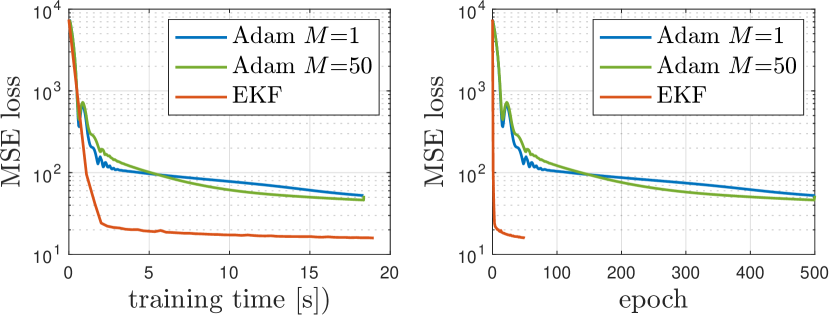
Figure 1: Fluid damper benchmark: MSE loss $\frac{1}{2N}\sum_{k=0}^{N-1}(y(k)-\hat{y}(k))^{2}$ evaluated at each epoch

We run the EKF-based learning method over $N_{e}=50$ epochs and compare the results to those obtained by solving the fully condensed problem (3) and the partially-condensed problem (11) with $M=50$ by using Adam with learning rate $l_{r}=0.005$ (the value of $l_{r}$ was chosen to get a good tradeoff between convergence speed and avoiding excessive oscillations).

Figure 1 shows the resulting MSE loss values in a typical run. When using EKF, after each epoch the initial condition $x_{0}$ is reconstructed by solving (23) with $\bar{u}(k)=u(k)$, $\bar{y}(k)=y(k)$ to evaluate the MSE loss. It is apparent that EKF reaches a good-quality model already after one pass through the training dataset and outperforms the other methods. Another advantage of EKF is that little effort was put on tuning the covariance matrices $Q_{y}$, $Q_{x}$, $Q_{\theta}$, $P(0|-1)$ for the EKF, while Adam required a careful tuning of the learning rate $l_{r}$ and also of the penalty $\gamma$ in case $M>1$.

Table 1 compares the fit results obtained by running the training methods on both the same RNN model structure and an LSTM model [16] with 4 hidden and 4 cell states (i.e., $n_{x}=8$ states) and the same output function $f_{y}$. The table shows the mean and standard deviation obtained over 20 runs (with $N_{e}=25$ used for EKF), starting from different initial model parameters, always computing the fit on the model with the lowest MSE obtained among all epochs. For further comparison, the best model Narx_6_2 reported in [35] provides a fit of 88.18% on training data and 85.15% on test data.

Table 1: Fluid damper benchmark: mean BFR (standard deviation) obtained over 20 runs

	BFR	Adam	Adam	EKF
		$M=1$	$M=50$
RNN	training	89.12 (1.83)	88.56 (1.85)	92.82 (0.33)
$n_{\theta}=107$	test	85.51 (2.89)	83.75 (4.71)	89.78 (0.58)
LSTM	training	89.60 (1.34)	87.47 (2.90)	92.63 (0.43)
$n_{\theta}=139$	test	85.56 (2.68)	80.62 (6.89)	88.97 (1.31)

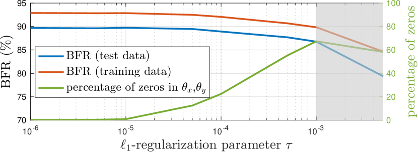
Figure 2: Fluid damper benchmark: BRF and sparsity of $\theta$ optimized by EKF vs $\ell_{1}$-regularization coefficient $\lambda$ (mean values over 20 runs)

Figure 2 shows the mean BRF obtained over 20 runs when training the RNN model (2b) under $\ell_{1}$-regularization $\lambda\|\theta\|_{1}$, introduced in the EKF as in (22b), for different values of $\lambda$. The figure also shows the mean percentage of zero entries in the resulting parameter vector $\theta$, where each entry $\theta_{i}$ such that $|\theta_{i}|\leq 10^{-3}$ is set to zero after EKF training. As expected, for increasing values of $\lambda$ the parameter vector gets more sparse, at the price of decreased prediction quality. For large values of $\lambda$ (roughly $\lambda>10^{-3}$), results start deteriorating, possibly due to the excessively large steps taken in (22b) that mine the convergence of the EKF.

6.2 Linear dynamical system with binary outputs

Consider $2000$ input/output pairs generated by the following linear system with binary outputs

$$\begin{array}[]{rcl}x(k+1)&=&\left[\begin{smallmatrix}.8&.2&-.1\\ 0&.9&.1\\ .1&-.1&.7\end{smallmatrix}\right]x(k)+\left[\begin{smallmatrix}-1\\ .5\\ 1\end{smallmatrix}\right]u(k)+\xi(k)\\[5.0pt] y(k)&=&\left\{\begin{array}[]{ll}1&\mbox{if}\ \left[\begin{smallmatrix}-2&1.5&0.5\end{smallmatrix}\right]x(k)-{\scriptsize{2}}+\zeta(k)\geq 0\\ 0&\mbox{otherwise}\end{array}\right.\end{array}$$

from $x(0)=0$, with the values of the input $u(k)$ changed with 90% probability from step $k$ to $k+1$ with a new value drawn from the uniform distribution on $[0,1]$. The disturbances $\xi_{i}(k),\zeta(k)\sim{\mathcal{N}}(0,\sigma^{2})$, $i=1,2,3$, are assumed independent. We consider the first $N=1000$ samples for training, the rest for testing the model. We want to fit an affine model ($L_{x}=L_{y}=1$) with sigmoidal output function $f_{1}^{y}(y)=1/(1+e^{-A_{1}^{y}[x^{\prime}(k)\ u(k)]^{\prime}-b_{1}^{y}})$. Output data are not scaled.

We run EKF ($N_{e}=25$) and Adam with $\rho_{x}=\rho_{\theta}=10^{-2}$, the initial weights randomly generated as in [33] and further scaled by a factor $\frac{1}{20}$, and the remaining settings as in Section 6.1, modified cross-entropy loss $\ell_{\rm CE\epsilon}$ for $\epsilon=0.005$, and EKF updates as in (18b). Adam is run with learning rates selected by trial and error as $l_{r}=0.01$ ($l_{r}=0.001$) for $M=1$ ($M=50$) to trade off convergence rate and variance. Table 2 shows the accuracy obtained by EKF and Adam (for $M=1$ and $M=50$) for increasing values of $\sigma$. Note that we kept $Q_{x}=10^{-10}$ in all tests, as we assumed not to know the intensity of the disturbances entering the system.

Table 2: Linear system with binary outputs: accuracy (%) on test (training) data (mean values over 20 runs)

$\sigma$	$M=1$	$M=50$	EKF
$0.000$	$97.37$ ($96.86$)	$83.06$ ($86.07$)	$98.02$ ($97.91$)
$0.001$	$95.00$ ($98.41$)	$86.88$ ($88.41$)	$95.33$ ($98.66$)
$0.010$	$97.38$ ($97.47$)	$87.65$ ($85.59$)	$97.99$ ($98.52$)
$0.100$	$94.84$ ($94.49$)	$74.64$ ($83.94$)	$94.56$ ($95.44$)
$0.200$	$91.49$ ($90.80$)	$80.37$ ($82.88$)	$93.71$ ($92.22$)

6.3 Nonlinear MPC benchmark: ethylene oxidation plant

We consider data generated from the ethylene oxidation plant model used as a nonlinear MPC benchmark in the Model Predictive Control Toolbox for MATLAB. A dataset of $2000$ samples is generated by numerically integrating the system of nonlinear ordinary differential equations of the plant model with high accuracy and collecting samples every $T_{s}=5$ s. The plant model has 4 states (gas density, C2H4 concentration, C2H4O concentration, and temperature in the reactor), one output ($y$ = C2H4O concentration), and two inputs ($u$ = total volumetric feed flow rate, that can be manipulated, and $v$ = C2H4 concentration of the feed, which is a measured disturbance). Half the dataset ($N=1000$ samples) is used to train a RNN with $L_{x}=3$ (i.e., a two-layer state-update neural network), $L_{y}=1$, $n_{x}=4$, $n_{1}^{x}=6$, $n_{2}^{x}=4$, affine output function, sigmoidal activation functions $f_{1}^{x},f_{2}^{x}$, and unit output function $f_{1}^{y}$. We run the EKF-based training algorithm by processing the dataset in $N_{e}=20$ epochs, which takes 4.54 s on the target machine. The resulting BRF is 94.33% on training data and 89.08% on test data.

The corresponding NLMPC controller, with MPC weights $W^{\Delta u}=0.1$, $W^{y}=10$, $u_{\rm min}=0.0704$, $u_{\rm max}=0.7042$, and prediction horizon $p=10$, is implemented using MATLAB’s fmincon solver with default parameters and no Jacobian information, warm-started from the shifted previous optimal solution. To close the feedback loop and get offset-free tracking of constant set-points, we apply EKF on line to estimate the state of the extended RNN model (25) with $B_{d}=0$, $C_{d}=1$ (output disturbance model); this corresponds to only adapting the bias coefficient $b_{1}^{y}$ in (2b), with covariances $E[\xi(k)\xi(k)^{\prime}]=0.01I$, $E[\eta(k)^{2}]=1$, $E[\zeta(k)^{2}]=0.01$, and $P(0|-1)=I$. The obtained closed-loop results are depicted in Figure 3, where it is apparent that a very good tracking is achieved despite the black-box RNN model used for prediction. The execution time ranges between 1.35 ms and 35.15 ms (8.86 ms on average) to solve the NLMPC problem and between 0.03 ms and 4.58 ms (0.15 ms on average) for state estimation.

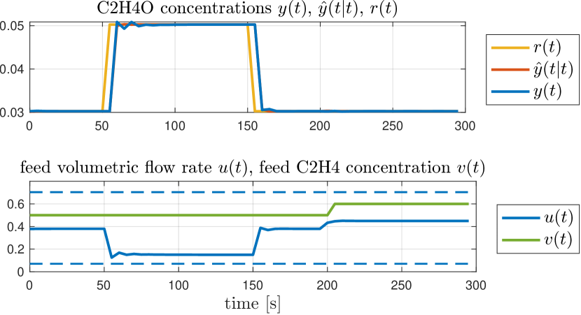
Figure 3: Ethilene oxidation benchmark: NLMPC results

7 Conclusions

We have shown that EKF is an effective way of learning control-oriented RNN models from input and output data, even in the case of general strongly convex and twice-differentiable loss functions and $\ell_{1}$-regularization. The approach is particularly suitable for online learning and model adaptation of recurrent neural networks and can be immediately extended to handle other classes of parametric nonlinear state-space models.

An interesting topic for future research is to study the conditions to impose on the RNN structure to make $x$ and $\theta$ observable, in particular to prevent over-parameterizing the model, and on how to choose model structure, loss function, and regularization terms to guarantee the asymptotic convergence of the filter.

References

• [1] J. Suykens, J. Vandewalle, and B. D. Moor, Artificial neural networks for modelling and control of non-linear systems.   Springer Science & Business Media, 1995.
• [2] V. Prasad and B. Bequette, “Nonlinear system identification and model reduction using artificial neural networks,” Computers & chemical engineering, vol. 27, no. 12, pp. 1741–1754, 2003.
• [3] D. Masti and A. Bemporad, “Learning nonlinear state-space models using autoencoders,” vol. 129, p. 109666, 2021.
• [4] R. Williams and J. Peng, “An efficient gradient-based algorithm for on-line training of recurrent network trajectories,” Neural computation, vol. 2, no. 4, pp. 490–501, 1990.
• [5] M. Forgione and D. Piga, “Model structures and fitting criteria for system identification with neural networks,” in 14th IEEE International Conference on Application of Information and Communication Technologies (AICT), Tashkent, Uzbekistan, 2020.
• [6] S. Singhal and L. Wu, “Training feed-forward networks with the extended Kalman algorithm,” in International Conference on Acoustics, Speech, and Signal Processing,, 1989, pp. 1187–1190.
• [7] G. Puskorius and L. Feldkamp, “Neurocontrol of nonlinear dynamical systems with Kalman filter trained recurrent networks,” IEEE Transactions on Neural Networks, vol. 5, no. 2, pp. 279–297, 1994.
• [8] X. Wang and Y. Huang, “Convergence study in extended Kalman filter-based training of recurrent neural networks,” IEEE Transactions on Neural Networks, vol. 22, no. 4, pp. 588–600, 2011.
• [9] R. Williams, “Training recurrent networks using the extended Kalman filter,” in IJCNN Int. Joint Conf. on Neural Networks, vol. 4, 1992, pp. 241–246.
• [10] M. Matthews and G. Moschytz, “Neural network nonlinear adaptive filtering using the extended Kalman filtering algorithm,” in Proc. of the Int. Neural Networks Conf., Paris, France, 1990, pp. 115–119.
• [11] M. Livstone, J. Farrell, and W. Baker, “A computationally efficient algorithm for training recurrent connectionist networks,” in Proc. American Control Conference, 1992, pp. 555–561.
• [12] D. Mirikitani and N. Nikolaev, “Efficient online recurrent connectionist learning with the ensemble Kalman filter,” Neurocomputing, vol. 73, no. 4-6, pp. 1024–1030, 2010.
• [13] Y. Iiguni, H. Sakai, and H. Tokumaru, “A real-time learning algorithm for a multilayered neural network based on the extended Kalman filter,” IEEE Transactions on Signal Processing, vol. 40, no. 4, pp. 959–966, 1992.
• [14] S. Hochreiter and J. Schmidhuber, “Long short-term memory,” Neural computation, vol. 9, no. 8, pp. 1735–1780, 1997.
• [15] L. Ljung, “Asymptotic behavior of the extended Kalman filter as a parameter estimator for linear systems,” IEEE Transactions on Automatic Control, vol. 24, no. 1, pp. 36–50, 1979.
• [16] F. Bonassi, E. Terzi, M. Farina, and R. Scattolini, “LSTM neural networks: Input to state stability and probabilistic safety verification,” in Learning for Dynamics and Control, Proceedings of Machine Learning Research, 2020, pp. 85–94.
• [17] J. Nocedal and S. Wright, Numerical Optimization, 2nd ed.   Springer, 2006.
• [18] A. Bemporad, “Training recurrent neural networks by sequential least squares and the alternating direction method of multipliers,” 2022, http://arxiv.org/abs/2112.15348.
• [19] P. J. Werbos, “Backpropagation through time: what it does and how to do it,” Proceedings of the IEEE, vol. 78, no. 10, pp. 1550–1560, 1990.
• [20] S. Hochreiter, “Recurrent neural net learning and vanishing gradient,” International Journal Of Uncertainity, Fuzziness and Knowledge-Based Systems, vol. 6, no. 2, pp. 107–116, 1998.
• [21] G. Hicks and W. Ray, “Approximation methods for optimal control synthesis,” The Canadian Journal of Chemical Engineering, vol. 49, no. 4, pp. 522–528, 1971.
• [22] A. Bemporad and G. Cimini, “Reduction of the number of variables in parametric constrained least-squares problems,” 2020, available on arXiv at http://arxiv.org/abs/2012.10423.
• [23] B. Evens, P. Latafat, A. Themelis, J. Suykens, and P. Patrinos, “Neural network training as an optimal control problem: An augmented Lagrangian approach,” in Proc. 60${}^{t}h$ Conf. Decision and Control, Austin, TX, USA, 2021, pp. 5136–5143.
• [24] H. Bock and K.-J. Plitt, “A multiple shooting algorithm for direct solution of optimal control problems,” IFAC Proceedings Volumes, vol. 17, no. 2, pp. 1603–1608, 1984.
• [25] D. Axehill, “Controlling the level of sparsity in MPC,” Systems & Control Letters, vol. 76, pp. 1–7, 2015.
• [26] J. Humpherys, P. Redd, and J. West, “A fresh look at the Kalman filter,” SIAM Review, vol. 54, no. 4, pp. 801–823, 2012.
• [27] M. Boutayeb, H. Rafaralahy, and M. Darouach, “Convergence analysis of the extended Kalman filter used as an observer for nonlinear deterministic discrete-time systems,” IEEE Transactions on Automatic Control, vol. 42, no. 4, pp. 581–586, 1997.
• [28] B. Gibbs, Advanced Kalman filtering, least-squares and modeling: a practical handbook.   John Wiley & Sons, 2011.
• [29] M. Vaccari, D. Bonvin, F. Pelagagge, and G. Pannocchia, “Offset-free economic MPC based on modifier adaptation: Investigation of several gradient-estimation techniques,” Processes, vol. 9, no. 5, p. 901, 2021.
• [30] J. Andersson, J. Gillis, G. Horn, J. Rawlings, and M. Diehl, “CasADi – A software framework for nonlinear optimization and optimal control,” Mathematical Programming Computation, vol. 11, no. 1, pp. 1–36, 2019.
• [31] A. Vaz and L. Vicente, “PSwarm: A hybrid solver for linearly constrained global derivative-free optimization,” Optimization Methods and Software, vol. 24, pp. 669–685, 2009, http://www.norg.uminho.pt/aivaz/pswarm/.
• [32] D. Kingma and J. Ba, “Adam: A method for stochastic optimization,” arXiv preprint arXiv:1412.6980, 2014.
• [33] X. Glorot and Y. Bengio, “Understanding the difficulty of training deep feedforward neural networks,” in Proc. 13${}^{t}h$ Int. Conf. Artificial Intelligence and Statistics, 2010, pp. 249–256.
• [34] J. Wang, A. Sano, T. Chen, and B. Huang, “Identification of Hammerstein systems without explicit parameterisation of non-linearity,” International Journal of Control, vol. 82, no. 5, pp. 937–952, 2009.
• [35] L. Ljung, System Identification Toolbox for MATLAB.   The Mathworks, Inc., https://www.mathworks.com/help/ident.