A novel control method for solving high-dimensional Hamiltonian systems through deep neural networks

Shaolin Ji Zhongtai Securities Institute for Financial Studies, Shandong University, 250100, China Shige Peng School of Mathematics, Shandong University, 250100, China Ying Peng Zhongtai Securities Institute for Financial Studies, Shandong University, 250100, China Xichuan Zhang School of Mathematics, Shandong University, 250100, China
Abstract

In this paper, we mainly focus on solving high-dimensional stochastic Hamiltonian systems with boundary condition, which is essentially a Forward Backward Stochastic Differential Equation (FBSDE in short), and propose a novel method from the view of the stochastic control. In order to obtain the approximated solution of the Hamiltonian system, we first introduce a corresponding stochastic optimal control problem such that the extended Hamiltonian system of the control problem is exactly what we need to solve, then we develop two different algorithms suitable for different cases of the control problem and approximate the stochastic control via deep neural networks. From the numerical results, comparing with the Deep FBSDE method developed previously from the view of solving FBSDEs, the novel algorithms converge faster, which means that they require fewer training steps, and demonstrate more stable convergences for different Hamiltonian systems.

Keywords stochastic Hamiltonian system, FBSDE, optimal control, PDE

1 Introduction

The theory of the Hamiltonian system is known as one of the dominant tools for the description of dynamic phenomenons in the field of physics and economics [1]. For example, in physics, the mechanical and electrical systems are usually represented as energy functions, which are at the same time Hamiltonian systems. Actually, the Hamiltonian system could reflect the laws of energy conservation and dissipation [1, 2].

A determined Hamiltonian system can be given as

{dxt=Hy(xt,yt)dt,dyt=Hx(xt,yt)dt,casesdsubscript𝑥𝑡subscript𝐻𝑦subscript𝑥𝑡subscript𝑦𝑡d𝑡otherwisedsubscript𝑦𝑡subscript𝐻𝑥subscript𝑥𝑡subscript𝑦𝑡d𝑡otherwise\begin{cases}\mathrm{d}x_{t}=H_{y}(x_{t},y_{t})\mathrm{d}t,\vspace{1ex}\\ \mathrm{d}y_{t}=H_{x}(x_{t},y_{t})\mathrm{d}t,\end{cases} (1.1)

where H(x,y):n×n:𝐻𝑥𝑦superscript𝑛superscript𝑛H(x,y):\mathbb{R}^{n}\times\mathbb{R}^{n}\rightarrow\mathbb{R} is a given real function called the Hamiltonian, Hx()subscript𝐻𝑥H_{x}(\cdot) and Hy()subscript𝐻𝑦H_{y}(\cdot) are partial derivatives of H()𝐻H(\cdot) with respect to x𝑥x and y𝑦y, respectively. When considering a terminal condition yT=Φx(xT)subscript𝑦𝑇subscriptΦ𝑥subscript𝑥𝑇y_{T}=\Phi_{x}(x_{T}) for a given function Φ:n:Φsuperscript𝑛\Phi:\mathbb{R}^{n}\rightarrow\mathbb{R}, (1.1) becomes a boundary problem.

For more complex environments where the physical system can not be represented with deterministic form, the Hamiltonian system is usually combined with a stochastic process. Here we consider a boundary problem of stochastic Hamiltonian system, as shown in the following,

{dxt=Hy(t,xt,yt,zt)dt+Hz(t,xt,yt,zt)dBt,dyt=Hx(t,xt,yt,zt)dtztdBt,x0=a,yT=Φx(xT),casesdsubscript𝑥𝑡subscript𝐻𝑦𝑡subscript𝑥𝑡subscript𝑦𝑡subscript𝑧𝑡d𝑡subscript𝐻𝑧𝑡subscript𝑥𝑡subscript𝑦𝑡subscript𝑧𝑡dsubscript𝐵𝑡otherwisedsubscript𝑦𝑡subscript𝐻𝑥𝑡subscript𝑥𝑡subscript𝑦𝑡subscript𝑧𝑡d𝑡subscript𝑧𝑡dsubscript𝐵𝑡otherwiseformulae-sequencesubscript𝑥0𝑎subscript𝑦𝑇subscriptΦ𝑥subscript𝑥𝑇otherwise\begin{cases}\mathrm{d}x_{t}=H_{y}(t,x_{t},y_{t},z_{t})\mathrm{d}t+H_{z}(t,x_{t},y_{t},z_{t})\mathrm{d}B_{t},\vspace{1ex}\\ -\mathrm{d}y_{t}=H_{x}(t,x_{t},y_{t},z_{t})\mathrm{d}t-z_{t}\mathrm{d}B_{t},\vspace{1ex}\\ x_{0}=a,\qquad y_{T}=-\Phi_{x}(x_{T}),\end{cases} (1.2)

which is essentially a fully coupled forward-backward stochastic differential equation (FBSDE in short). Many research work have studied the solutions of FBSDEs and the eigenvalue of the Hamiltonian systems [3, 4, 5, 6, 7, 8, 9, 10, 11]. The significance of studying this kind of Hamiltonian system is that on the one hand it can be applied in solving the stochastic optimal control problems via the well-known stochastic maximum principle [12, 13]; on the other hand, it helps to obtain the solutions of nonlinear partial differential equations (PDEs in short) according to the connection between the FBSDEs and the PDEs  [11].

In most cases, it is difficult to obtain the explicit solution of the Hamiltonian system (1.2), thus numerical methods should be studied. As (1.2) is essentially a FBSDE, an intuitive way is to solve (1.2) from the perspective of FBSDEs. Therefore, numerical methods for solving the FBSDEs can be applied  [14, 15, 16, 17, 18, 19, 20, 21, 22, 23, 8] , such as the PDE methods, the probabilistic methods, etc. However, most of the traditional numerical methods can not deal with high-dimensional problems. Moreover, it is worth to point out that solving the fully coupled FBSDEs numerically has been a much more challenging problem than the general FBSDEs, even for low dimensional cases. Recently, with the application of the deep learning technique in a wide range of areas, numerical methods based on deep neural networks have been proposed to solve high-dimensional Backward Stochastic Differential Equations (BSDEs in short) and FBSDEs and achieved remarkable success. Among them, a breakthrough work was developed by  [24, 25], the main idea is to reformulate the BSDE into a stochastic optimal control problem by rewriting the backward process into a forward form and taking the terminal error as the cost functional, then the solution of the BSDE is approximated by deep neural network. Other different deep learning algorithms are proposed to solve the BSDEs and related PDEs [26, 27, 28, 29], where they also focus on approximating the solution of the BSDE (or PDE) with the deep neural network. For solving coupled and fully coupled FBSDEs, [30, 31] developed numerical algorithms which are also inspired by  [24, 25].

In this paper, we propose a novel method to solve the Hamiltonian system (1.2) via deep learning. As equation (1.2) is at the same time a fully coupled FBSDE, this method is also suitable for solving fully coupled FBSDEs. However, different from the above mentioned deep learning methods which aim to solve the FBSDEs directly, we first look for the corresponding stochastic optimal control problem of the Hamiltonian system, such that the extended Hamiltonian system of the stochastic control problem is exactly what we need to solve. Then we approximate the optimal control with deep neural networks. In order to solve the optimal control problem, two different cases are considered which correspond to two different algorithms. The first algorithm (Algorithm 1) deals with the case where the function f(t,x,u,v)𝑓𝑡𝑥𝑢𝑣f(t,x,u,v) defined in (2.5) has an explicit form. For the case that f(t,x,u,v)𝑓𝑡𝑥𝑢𝑣f(t,x,u,v) cannot be expressed explicitly, the original control problem is transformed to a double objective optimization problem and we develop the second algorithm (Algorithm 2) to solve it. Finally, the numerical solutions (yt,zt)subscript𝑦𝑡subscript𝑧𝑡(y_{t},z_{t}) of (1.2) are obtained by calculating the solution of the extended Hamiltonian system for the optimal control according to the stochastic maximum principle.

We also compare the results of our novel proposed algorithms with that of the algorithm developed in our previous work [31] ( called the Deep FBSDE method here), which can be used to solve the Hamiltonian system from the view of the FBSDEs. Comparing with the Deep FBSDE method, the novel algorithms have two advantages. The first advantage is that less numbers of iteration steps are required to achieve convergent results. When the Deep FBSDE method converges, it needs more iterations to achieve a convergent result. The second advantage is that our proposed algorithms have more stable convergences. For some Hamiltonian systems, the Deep FBSDE method is easier to diverge with the same piecewise decay learning rate as our novel proposed algorithms. The details can be referred to the numerical results in section 4.

This paper is organized as follows. In section 2, we describe the Hamiltonian system that we aim to solve, and introduce its corresponding stochastic optimal control problem. In section 3, we introduce two schemes to solve the stochastic control problem according to whether the function f(t,x,u,v)𝑓𝑡𝑥𝑢𝑣f(t,x,u,v) defined in (2.5) has an explicit form, and then give the corresponding neural network architectures. The numerical results for different examples are shown in section 4, and a brief conclusion is made in section 5.

2 Problem formulation

In this section, we first introduce the stochastic Hamiltonian system that we aim to solve, then we show that solving this kind of stochastic Hamiltonian systems is equivalent to solving a stochastic optimal control problem.

2.1 The stochastic Hamiltonian system

Let T>0𝑇0T>0, (Ω,,𝔽,)Ω𝔽(\Omega,\mathcal{F},\mathbb{F},\mathbb{P}) be a filtered probability space, in which B:[0,T]×Ωd:𝐵0𝑇Ωsuperscript𝑑B:[0,T]\times\Omega\rightarrow\mathbb{R}^{d} is a d𝑑d-dimensional standard 𝔽𝔽\mathbb{F}-Brownian motion; 𝔽={t}0tT𝔽subscriptsubscript𝑡0𝑡𝑇\mathbb{F}=\{\mathcal{F}_{t}\}_{0\leq t\leq T} is the natural filtration generated by the Brownian motion B𝐵B Suppose that (Ω,,)Ω(\Omega,\mathcal{F},\mathbb{P}) is complete, 0subscript0\mathcal{F}_{0} contains all the \mathbb{P}-null sets in \mathcal{F} and 𝔽𝔽\mathbb{F} is right continuous.

For z1,z2n×dsuperscript𝑧1superscript𝑧2superscript𝑛𝑑z^{1},z^{2}\in\mathbb{R}^{n\times d}, define z1,z2=tr(z1(z2)T)superscript𝑧1superscript𝑧2trsuperscript𝑧1superscriptsuperscript𝑧2T\left\langle z^{1},z^{2}\right\rangle=\mbox{tr}(z^{1}(z^{2})^{\operatorname{T}}{}) and |z|2=z,zsuperscript𝑧2𝑧𝑧|z|^{2}=\left\langle z,z\right\rangle. The space of all mean square-integrable tsubscript𝑡\mathcal{F}_{t}-adapted and nsuperscript𝑛\mathbb{R}^{n}-valued processes will be denoted by M2(0,T;n)superscript𝑀20𝑇superscript𝑛M^{2}(0,T;\mathbb{R}^{n}), which is a Hilbert space with the norm

v()=(𝔼[0T|v(t)|2𝑑t])1/2norm𝑣superscript𝔼delimited-[]superscriptsubscript0𝑇superscript𝑣𝑡2differential-d𝑡12\|v(\cdot)\|=\Big{(}\mathbb{E}\big{[}\int_{0}^{T}|v(t)|^{2}dt\big{]}\Big{)}^{1/2}

and

L2(Ω,t,){ξ|ξn is t-measurable and 𝔼[|ξ|2]<}.superscript𝐿2Ωsubscript𝑡conditional-set𝜉𝜉superscript𝑛 is subscript𝑡-measurable and 𝔼delimited-[]superscript𝜉2L^{2}(\Omega,\mathcal{F}_{t},\mathbb{P})\triangleq\left\{\xi|\xi\in\mathbb{R}^{n}\mbox{ is }\mathcal{F}_{t}\mbox{-measurable and }\mathbb{E}\left[|\xi|^{2}\right]<\infty\right\}.

Let

H:[0,T]×n×n×n×d,:𝐻0𝑇superscript𝑛superscript𝑛superscript𝑛𝑑H:[0,T]\times\mathbb{R}^{n}\times\mathbb{R}^{n}\times\mathbb{R}^{n\times d}\rightarrow\mathbb{R}, (2.1)

be a C2superscript𝐶2C^{2} real function of (x,y,z)𝑥𝑦𝑧(x,y,z), called a Hamiltonian and let

Φ:n,:Φsuperscript𝑛\Phi:\mathbb{R}^{n}\rightarrow\mathbb{R}, (2.2)

be a C1superscript𝐶1C^{1} real function of x𝑥x. In our context, unless otherwise stated, we always assume that the Hamiltonian H𝐻H is strictly convex with respect to y𝑦y and z𝑧z.

Consider the following stochastic Hamiltonian system:

{dxt=Hy(t,xt,yt,zt)dt+Hz(t,xt,yt,zt)dBt,dyt=Hx(t,xt,yt,zt)dtztdBt,x0=a,yT=Φx(xT),casesdsubscript𝑥𝑡subscript𝐻𝑦𝑡subscript𝑥𝑡subscript𝑦𝑡subscript𝑧𝑡d𝑡subscript𝐻𝑧𝑡subscript𝑥𝑡subscript𝑦𝑡subscript𝑧𝑡dsubscript𝐵𝑡otherwisedsubscript𝑦𝑡subscript𝐻𝑥𝑡subscript𝑥𝑡subscript𝑦𝑡subscript𝑧𝑡d𝑡subscript𝑧𝑡dsubscript𝐵𝑡otherwiseformulae-sequencesubscript𝑥0𝑎subscript𝑦𝑇subscriptΦ𝑥subscript𝑥𝑇otherwise\begin{cases}\mathrm{d}x_{t}=H_{y}(t,x_{t},y_{t},z_{t})\mathrm{d}t+H_{z}(t,x_{t},y_{t},z_{t})\mathrm{d}B_{t},\vspace{1ex}\\ -\mathrm{d}y_{t}=H_{x}(t,x_{t},y_{t},z_{t})\mathrm{d}t-z_{t}\mathrm{d}B_{t},\vspace{1ex}\\ x_{0}=a,\qquad y_{T}=-\Phi_{x}(x_{T}),\end{cases} (2.3)

where Hxsubscript𝐻𝑥H_{x}, Hysubscript𝐻𝑦H_{y}, Hzsubscript𝐻𝑧H_{z} are derivatives of H𝐻H with respect to x𝑥x, y𝑦y, z𝑧z, respectively. And the above system is essentially a special kind of fully coupled FBSDEs.

Set

w=(xyz)n×n×n×d,A(t,w)=(HxHyHz)(t,w),formulae-sequence𝑤matrix𝑥𝑦𝑧superscript𝑛superscript𝑛superscript𝑛𝑑𝐴𝑡𝑤matrixsubscript𝐻𝑥subscript𝐻𝑦subscript𝐻𝑧𝑡𝑤w=\begin{pmatrix}x\\ y\\ z\end{pmatrix}\in\mathbb{R}^{n}\times\mathbb{R}^{n}\times\mathbb{R}^{n\times d},\qquad A(t,w)=\begin{pmatrix}-H_{x}\\ H_{y}\\ H_{z}\end{pmatrix}(t,w),

and

w1,w2=x1,x2+y1,y2+z1,z2.superscript𝑤1superscript𝑤2superscript𝑥1superscript𝑥2superscript𝑦1superscript𝑦2superscript𝑧1superscript𝑧2\left\langle w^{1},w^{2}\right\rangle=\left\langle x^{1},x^{2}\right\rangle+\left\langle y^{1},y^{2}\right\rangle+\left\langle z^{1},z^{2}\right\rangle.
Definition 2.1.

A triple of process (x(),y(),z()):[0,T]×Ωn×n×n×d:𝑥𝑦𝑧0𝑇Ωsuperscript𝑛superscript𝑛superscript𝑛𝑑(x(\cdot),y(\cdot),z(\cdot)):[0,T]\times\Omega\rightarrow\mathbb{R}^{n}\times\mathbb{R}^{n}\times\mathbb{R}^{n\times d} is called an adapted solution of (2.3), if (x(),y(),z())M2(0,T;n×n×n×d)𝑥𝑦𝑧superscript𝑀20𝑇superscript𝑛superscript𝑛superscript𝑛𝑑(x(\cdot),y(\cdot),z(\cdot))\in M^{2}(0,T;\mathbb{R}^{n}\times\mathbb{R}^{n}\times\mathbb{R}^{n\times d}), and it satisfies (2.3).

Assumption 1.

For any w,wn×n×n×d𝑤superscript𝑤superscript𝑛superscript𝑛superscript𝑛𝑑w,w^{\prime}\in\mathbb{R}^{n}\times\mathbb{R}^{n}\times\mathbb{R}^{n\times d} and x,xn𝑥superscript𝑥superscript𝑛x,x^{\prime}\in\mathbb{R}^{n},

  • (i)

    there exists a constant β1>0subscript𝛽10\beta_{1}>0, such that

    |A(t,w)A(t,w)|β1|ww|,𝐴𝑡𝑤𝐴𝑡superscript𝑤subscript𝛽1𝑤superscript𝑤\begin{array}[]{c}|A(t,w)-A(t,w^{\prime})|\leq\beta_{1}|w-w^{\prime}|,\vspace{1ex}\\ \end{array}

    and

    |Φx(x)Φx(x)|β1|xx|.subscriptΦ𝑥𝑥subscriptΦ𝑥superscript𝑥subscript𝛽1𝑥superscript𝑥|\Phi_{x}(x)-\Phi_{x}(x^{\prime})|\leq\beta_{1}|x-x^{\prime}|.
  • (ii)

    there exists a constant β2>0subscript𝛽20\beta_{2}>0, such that the following monotonic conditions hold.

    A(t,w)A(t,w),ww𝐴𝑡𝑤𝐴𝑡superscript𝑤𝑤superscript𝑤\displaystyle\langle A(t,w)-A(t,w^{\prime}),w-w^{\prime}\rangle β2|ww|2absentsubscript𝛽2superscript𝑤superscript𝑤2\displaystyle\leq-\beta_{2}|w-w^{\prime}|^{2}
    Φx(x)+Φx(x),xxsubscriptΦ𝑥𝑥subscriptΦ𝑥superscript𝑥𝑥superscript𝑥\displaystyle\langle-\Phi_{x}(x)+\Phi_{x}(x^{\prime}),x-x^{\prime}\rangle β2|xx|2.absentsubscript𝛽2superscript𝑥superscript𝑥2\displaystyle\geq\beta_{2}|x-x^{\prime}|^{2}.

As equation (2.3) is at the same time a fully coupled FBSDE, we recall the following existence and uniqueness theorem in [3, 4].

Theorem 1 (Theorem 3.1 in [3]).

Let Assumption 1 hold. Then there exists a unique adapted solution (x(),y(),z())𝑥𝑦𝑧(x(\cdot),y(\cdot),z(\cdot)) for (2.3).

Recently, numerical algorithms for solving the BSDEs and FBSDEs with deep learning method  [24, 25, 30, 31] have been proposed and demonstrated remarkable performance. The main idea is to reformulate the BSDE into a stochastic optimal control problem, where the solution z𝑧z of the BSDE is regarded as a control and approximated with deep neural network, and the terminal error is taken as the cost functional. Other different numerical algorithms have also been developed for solving the FBSDEs and the related PDEs [26, 27, 28, 29], which also regard the solution of the FBSDE (y𝑦y or z𝑧z) as a control and approximate it with appropriate loss function.

2.2 A novel method to solve the stochastic Hamiltonian system

As noted in the previous sections, the stochastic Hamiltonian system (2.3) is essentially a fully coupled FBSDE and can be solved through the methods for solving the FBSDEs. In this paper, we develop a novel method for solving the Hamiltonian system(2.3). Different from the above mentioned algorithms for solving the BSDEs or FBSDEs, our main idea is to find the corresponding stochastic optimal control problem of the stochastic Hamiltonian system, and then directly apply the deep learning method to solve the control problem.

x,y,un,z,vn×dformulae-sequencefor-all𝑥𝑦𝑢superscript𝑛𝑧𝑣superscript𝑛𝑑\forall x,y,u\in\mathbb{R}^{n},z,v\in\mathbb{R}^{n\times d}, set

F(t,x,u,v,y,z)=y,u+z,vH(t,x,y,z)𝐹𝑡𝑥𝑢𝑣𝑦𝑧𝑦𝑢𝑧𝑣𝐻𝑡𝑥𝑦𝑧F(t,x,u,v,y,z)=\langle y,u\rangle+\langle z,v\rangle-H(t,x,y,z) (2.4)

and

f(t,x,u,v)=maxy,zF(t,x,u,v,y,z).𝑓𝑡𝑥𝑢𝑣subscript𝑦𝑧𝐹𝑡𝑥𝑢𝑣𝑦𝑧f(t,x,u,v)=\max_{y,z}F(t,x,u,v,y,z). (2.5)

Here f(t,x,u,v)𝑓𝑡𝑥𝑢𝑣f(t,x,u,v) is the Legendre-Fenchel transform of H(t,x,y,z)𝐻𝑡𝑥𝑦𝑧H(t,x,y,z) with respect to (y,z)𝑦𝑧(y,z). Due to the differentiability and strict convexity of the Hamiltonian H𝐻H, f𝑓f is also differential and strictly convex with respect to u𝑢u and v𝑣v [32].

Consider the following control system,

{dxt=utdt+vtdBt,x0=a,casesdsubscript𝑥𝑡subscript𝑢𝑡d𝑡subscript𝑣𝑡dsubscript𝐵𝑡otherwisesubscript𝑥0𝑎otherwise\begin{cases}\mathrm{d}x_{t}=u_{t}\mathrm{d}t+v_{t}\mathrm{d}B_{t},\vspace{1ex}\\ x_{0}=a,\end{cases} (2.6)

and the cost functional is given as

J(u(),v())=𝔼[0Tf(t,xt,ut,vt)dt+Φ(xT)],𝐽𝑢𝑣𝔼delimited-[]superscriptsubscript0𝑇𝑓𝑡subscript𝑥𝑡subscript𝑢𝑡subscript𝑣𝑡differential-d𝑡Φsubscript𝑥𝑇J(u(\cdot),v(\cdot))=\mathbb{E}\left[\int_{0}^{T}f(t,x_{t},u_{t},v_{t})\mathrm{d}t+\Phi(x_{T})\right], (2.7)

where the controls u()𝑢u(\cdot) and v()𝑣v(\cdot) belong to M2(0,T;n)superscript𝑀20𝑇superscript𝑛M^{2}(0,T;\mathbb{R}^{n}) and M2(0,T;n×d)superscript𝑀20𝑇superscript𝑛𝑑M^{2}(0,T;\mathbb{R}^{n\times d}), respectively. The set of all admissible controls is denoted by 𝒰ad[0,T]subscript𝒰𝑎𝑑0𝑇\mathcal{U}_{ad}[0,T]. Any (u(),v())𝒰ad[0,T]superscript𝑢superscript𝑣subscript𝒰𝑎𝑑0𝑇(u^{*}(\cdot),v^{*}(\cdot))\in\mathcal{U}_{ad}[0,T] satisfying

J(u(),v())=inf(u(),v())𝒰ad[0,T]J(u(),v())𝐽superscript𝑢superscript𝑣subscriptinfimum𝑢𝑣subscript𝒰𝑎𝑑0𝑇𝐽𝑢𝑣J(u^{*}(\cdot),v^{*}(\cdot))=\inf_{(u(\cdot),v(\cdot))\in\mathcal{U}_{ad}[0,T]}J(u(\cdot),v(\cdot)) (2.8)

is called an optimal control. The corresponding state trajectory x()superscript𝑥x^{*}(\cdot) is called an optimal trajectory and the corresponding triple (x(),u(),v())superscript𝑥superscript𝑢superscript𝑣(x^{*}(\cdot),u^{*}(\cdot),v^{*}(\cdot)) is called an optimal triple.

In the following we prove that solving the stochastic Hamiltonian system (2.3) is equivalent to solving the stochastic optimal control problem (2.6)-(2.7).

We need the following assumption.

Assumption 2.

f(t,x,u,v)𝑓𝑡𝑥𝑢𝑣f(t,x,u,v) is continuously differentiable with respect to x𝑥x, u𝑢u, v𝑣v, and

|fx(t,x,u,v)|subscript𝑓𝑥𝑡𝑥𝑢𝑣\displaystyle|f_{x}(t,x,u,v)| C(|x|+|u|+|v|+1),absent𝐶𝑥𝑢𝑣1\displaystyle\leq C(|x|+|u|+|v|+1),\vspace{1ex}
|fu(t,x,u,v)|subscript𝑓𝑢𝑡𝑥𝑢𝑣\displaystyle|f_{u}(t,x,u,v)| C(|x|+|u|+|v|+1),absent𝐶𝑥𝑢𝑣1\displaystyle\leq C(|x|+|u|+|v|+1),\vspace{1ex}
|fv(t,x,u,v)|subscript𝑓𝑣𝑡𝑥𝑢𝑣\displaystyle|f_{v}(t,x,u,v)| C(|x|+|u|+|v|+1),absent𝐶𝑥𝑢𝑣1\displaystyle\leq C(|x|+|u|+|v|+1),\vspace{1ex}
|f(t,0,0,0)|𝑓𝑡000\displaystyle|f(t,0,0,0)| Cabsent𝐶\displaystyle\leq C

for some given C>0𝐶0C>0.

Theorem 2.

Let H𝐻H be a given C2superscript𝐶2C^{2} real function and strictly convex with respect to y𝑦y and z𝑧z. The derivatives of H𝐻H and ΦΦ\Phi satisfy Assumption 1; f𝑓f satisfies Assumption 2. Suppose that (x(),u(),v())superscript𝑥superscript𝑢superscript𝑣(x^{*}(\cdot),u^{*}(\cdot),v^{*}(\cdot)) is the optimal triple of the optimal control problem (2.6)-(2.7). Then (x(),y(),z())superscript𝑥superscript𝑦superscript𝑧(x^{*}(\cdot),y^{*}(\cdot),z^{*}(\cdot)) uniquely solves the Hamiltonian system (2.3), where y()superscript𝑦y^{*}(\cdot) can be given as

ytsuperscriptsubscript𝑦𝑡\displaystyle y_{t}^{*} =𝔼[tTfx(s,xs,us,vs)dsΦx(xT)|t],absent𝔼delimited-[]superscriptsubscript𝑡𝑇subscript𝑓𝑥𝑠superscriptsubscript𝑥𝑠subscriptsuperscript𝑢𝑠subscriptsuperscript𝑣𝑠d𝑠conditionalsubscriptΦ𝑥subscriptsuperscript𝑥𝑇subscript𝑡\displaystyle=\mathbb{E}\left[\int_{t}^{T}-f_{x}(s,x_{s}^{*},u^{*}_{s},v^{*}_{s})\mathrm{d}s-\Phi_{x}(x^{*}_{T})\Big{|}\mathcal{F}_{t}\right], (2.9)

and z()superscript𝑧z^{*}(\cdot) can be solved by this following BSDE

{dyt=fx(t,xt,ut,vt)dtztdBt,yT=Φx(xT),t[0,T].casesdsuperscriptsubscript𝑦𝑡subscript𝑓𝑥𝑡subscriptsuperscript𝑥𝑡subscriptsuperscript𝑢𝑡subscriptsuperscript𝑣𝑡d𝑡superscriptsubscript𝑧𝑡dsubscript𝐵𝑡formulae-sequencesuperscriptsubscript𝑦𝑇subscriptΦ𝑥subscriptsuperscript𝑥𝑇𝑡0𝑇\left\{\begin{array}[]{l}-\mathrm{d}y_{t}^{*}=-f_{x}(t,x^{*}_{t},u^{*}_{t},v^{*}_{t})\mathrm{d}t-z_{t}^{*}\mathrm{d}B_{t},\vspace{1ex}\\ y_{T}^{*}=-\Phi_{x}(x^{*}_{T}),\qquad t\in[0,T].\end{array}\right. (2.10)
Proof.

Set

h(t,x,u,v,y,z)=y,u+z,vf(t,x,u,v).𝑡𝑥𝑢𝑣𝑦𝑧𝑦𝑢𝑧𝑣𝑓𝑡𝑥𝑢𝑣h(t,x,u,v,y,z)=\langle y,u\rangle+\langle z,v\rangle-f(t,x,u,v). (2.11)

Under our assumptions, for any optimal triple (x(),u(),v())superscript𝑥superscript𝑢superscript𝑣(x^{*}(\cdot),u^{*}(\cdot),v^{*}(\cdot)) of the optimal control problem (2.6)-(2.7), we have the following extended stochastic Hamiltonian system through the well-known stochastic maximum principle (SMP in short) ( e.g. Theorem 4.1 in [12]),

{dxt=utdt+vtdBt,dyt=hx(t,xt,ut,vt,yt,zt)dtztdBt,x0=a,yT=Φx(xT),t[0,T],casesdsuperscriptsubscript𝑥𝑡superscriptsubscript𝑢𝑡d𝑡superscriptsubscript𝑣𝑡dsubscript𝐵𝑡otherwisedsuperscriptsubscript𝑦𝑡subscript𝑥𝑡subscriptsuperscript𝑥𝑡subscriptsuperscript𝑢𝑡subscriptsuperscript𝑣𝑡subscriptsuperscript𝑦𝑡subscriptsuperscript𝑧𝑡d𝑡superscriptsubscript𝑧𝑡dsubscript𝐵𝑡otherwiseformulae-sequencesuperscriptsubscript𝑥0𝑎formulae-sequencesuperscriptsubscript𝑦𝑇subscriptΦ𝑥subscriptsuperscript𝑥𝑇𝑡0𝑇otherwise\begin{cases}\mathrm{d}x_{t}^{*}=u_{t}^{*}\mathrm{d}t+v_{t}^{*}\mathrm{d}B_{t},\vspace{1ex}\\ -\mathrm{d}y_{t}^{*}=h_{x}(t,x^{*}_{t},u^{*}_{t},v^{*}_{t},y^{*}_{t},z^{*}_{t})\mathrm{d}t-z_{t}^{*}\mathrm{d}B_{t},\vspace{1ex}\\ x_{0}^{*}=a,\qquad y_{T}^{*}=-\Phi_{x}(x^{*}_{T}),\qquad t\in[0,T],\end{cases} (2.12)

and

h(t,xt,ut,vt,yt,zt)=maxun,vn×dh(t,xt,u,v,yt,zt),a.e.t[0,T].formulae-sequence𝑡subscriptsuperscript𝑥𝑡subscriptsuperscript𝑢𝑡subscriptsuperscript𝑣𝑡subscriptsuperscript𝑦𝑡subscriptsuperscript𝑧𝑡subscriptformulae-sequence𝑢superscript𝑛𝑣superscript𝑛𝑑𝑡subscriptsuperscript𝑥𝑡𝑢𝑣subscriptsuperscript𝑦𝑡subscriptsuperscript𝑧𝑡𝑎𝑒𝑡0𝑇h(t,x^{*}_{t},u^{*}_{t},v^{*}_{t},y^{*}_{t},z^{*}_{t})=\max_{u\in\mathbb{R}^{n},\\ v\in\mathbb{R}^{n\times d}}h(t,x^{*}_{t},u,v,y^{*}_{t},z^{*}_{t}),\ a.e.\ t\in[0,T]. (2.13)

The solution of the extended stochastic Hamiltonian system (2.12)-(2.13) is a 5-tuple (x(),u(),v(),y(),z())superscript𝑥superscript𝑢superscript𝑣superscript𝑦superscript𝑧(x^{*}(\cdot),u^{*}(\cdot),v^{*}(\cdot),y^{*}(\cdot),z^{*}(\cdot)).

By Theorem 12.2 in [32], we have the inverse Legendre-Fenchel transform of (2.5):

H(t,x,y,z)=maxu,vh(t,x,u,v,y,z).𝐻𝑡𝑥𝑦𝑧subscript𝑢𝑣𝑡𝑥𝑢𝑣𝑦𝑧H(t,x,y,z)=\max_{u,v}h(t,x,u,v,y,z). (2.14)

Because h(t,x,u,v,y,z)𝑡𝑥𝑢𝑣𝑦𝑧h(t,x,u,v,y,z) is strictly concave in u,v𝑢𝑣u,v, it yields that the maximum point (ut,vt)subscriptsuperscript𝑢𝑡subscriptsuperscript𝑣𝑡(u^{*}_{t},v^{*}_{t}) of (2.13) is uniquely determined by (xt,yt,zt)subscriptsuperscript𝑥𝑡subscriptsuperscript𝑦𝑡subscriptsuperscript𝑧𝑡(x^{*}_{t},y^{*}_{t},z^{*}_{t}) due to the implicit function existence theorem:

utsubscriptsuperscript𝑢𝑡\displaystyle u^{*}_{t} =u¯(t,xt,yt,zt),absent¯𝑢𝑡subscriptsuperscript𝑥𝑡subscriptsuperscript𝑦𝑡subscriptsuperscript𝑧𝑡\displaystyle=\bar{u}(t,x^{*}_{t},y^{*}_{t},z^{*}_{t}), (2.15)
vtsubscriptsuperscript𝑣𝑡\displaystyle v^{*}_{t} =v¯(t,xt,yt,zt),absent¯𝑣𝑡subscriptsuperscript𝑥𝑡subscriptsuperscript𝑦𝑡subscriptsuperscript𝑧𝑡\displaystyle=\bar{v}(t,x^{*}_{t},y^{*}_{t},z^{*}_{t}),

and u¯,v¯¯𝑢¯𝑣\bar{u},\bar{v} are differentiable functions. By (2.14),

H(t,xt,yt,zt)𝐻𝑡subscriptsuperscript𝑥𝑡subscriptsuperscript𝑦𝑡subscriptsuperscript𝑧𝑡\displaystyle H(t,x^{*}_{t},y^{*}_{t},z^{*}_{t}) =h(t,xt,u¯(t,xt,yt,zt),v¯(t,xt,yt,zt),yt,zt),absent𝑡subscriptsuperscript𝑥𝑡¯𝑢𝑡subscriptsuperscript𝑥𝑡subscriptsuperscript𝑦𝑡subscriptsuperscript𝑧𝑡¯𝑣𝑡subscriptsuperscript𝑥𝑡subscriptsuperscript𝑦𝑡subscriptsuperscript𝑧𝑡subscriptsuperscript𝑦𝑡subscriptsuperscript𝑧𝑡\displaystyle=h(t,x^{*}_{t},\bar{u}(t,x^{*}_{t},y^{*}_{t},z^{*}_{t}),\bar{v}(t,x^{*}_{t},y^{*}_{t},z^{*}_{t}),y^{*}_{t},z^{*}_{t}), (2.16)

which leads to

f(t,xt,u¯(t,xt,yt,zt),v¯(t,xt,yt,zt))𝑓𝑡subscriptsuperscript𝑥𝑡¯𝑢𝑡subscriptsuperscript𝑥𝑡subscriptsuperscript𝑦𝑡subscriptsuperscript𝑧𝑡¯𝑣𝑡subscriptsuperscript𝑥𝑡subscriptsuperscript𝑦𝑡subscriptsuperscript𝑧𝑡\displaystyle f(t,x^{*}_{t},\bar{u}(t,x^{*}_{t},y^{*}_{t},z^{*}_{t}),\bar{v}(t,x^{*}_{t},y^{*}_{t},z^{*}_{t})) (2.17)
=\displaystyle= yt,u¯(t,xt,yt,zt)+zt,v¯(t,xt,yt,zt)H(t,xt,yt,zt).subscriptsuperscript𝑦𝑡¯𝑢𝑡subscriptsuperscript𝑥𝑡subscriptsuperscript𝑦𝑡subscriptsuperscript𝑧𝑡subscriptsuperscript𝑧𝑡¯𝑣𝑡subscriptsuperscript𝑥𝑡subscriptsuperscript𝑦𝑡subscriptsuperscript𝑧𝑡𝐻𝑡subscriptsuperscript𝑥𝑡subscriptsuperscript𝑦𝑡subscriptsuperscript𝑧𝑡\displaystyle\langle y^{*}_{t},\bar{u}(t,x^{*}_{t},y^{*}_{t},z^{*}_{t})\rangle+\langle z^{*}_{t},\bar{v}(t,x^{*}_{t},y^{*}_{t},z^{*}_{t})\rangle-H(t,x^{*}_{t},y^{*}_{t},z^{*}_{t}).

Thus, the derivatives of f(t,x,u,v)𝑓𝑡𝑥𝑢𝑣f(t,x,u,v) with respect to u,v𝑢𝑣u,v are

fu(t,xt,u¯(t,xt,yt,zt),v¯(t,xt,yt,zt))=yt,subscript𝑓𝑢𝑡subscriptsuperscript𝑥𝑡¯𝑢𝑡subscriptsuperscript𝑥𝑡subscriptsuperscript𝑦𝑡subscriptsuperscript𝑧𝑡¯𝑣𝑡subscriptsuperscript𝑥𝑡subscriptsuperscript𝑦𝑡subscriptsuperscript𝑧𝑡subscriptsuperscript𝑦𝑡\displaystyle f_{u}(t,x^{*}_{t},\bar{u}(t,x^{*}_{t},y^{*}_{t},z^{*}_{t}),\bar{v}(t,x^{*}_{t},y^{*}_{t},z^{*}_{t}))=y^{*}_{t}, (2.18)
fv(t,xt,u¯(t,xt,yt,zt),v¯(t,xt,yt,zt))=zt.subscript𝑓𝑣𝑡subscriptsuperscript𝑥𝑡¯𝑢𝑡subscriptsuperscript𝑥𝑡subscriptsuperscript𝑦𝑡subscriptsuperscript𝑧𝑡¯𝑣𝑡subscriptsuperscript𝑥𝑡subscriptsuperscript𝑦𝑡subscriptsuperscript𝑧𝑡subscriptsuperscript𝑧𝑡\displaystyle f_{v}(t,x^{*}_{t},\bar{u}(t,x^{*}_{t},y^{*}_{t},z^{*}_{t}),\bar{v}(t,x^{*}_{t},y^{*}_{t},z^{*}_{t}))=z^{*}_{t}.

It can be verified that

Hx(t,xt,yt,zt)=subscript𝐻𝑥𝑡subscriptsuperscript𝑥𝑡subscriptsuperscript𝑦𝑡subscriptsuperscript𝑧𝑡absent\displaystyle H_{x}(t,x^{*}_{t},y^{*}_{t},z^{*}_{t})= fx(t,xt,u¯(t,xt,yt,zt),v¯(t,xt,yt,zt))subscript𝑓𝑥𝑡subscriptsuperscript𝑥𝑡¯𝑢𝑡subscriptsuperscript𝑥𝑡subscriptsuperscript𝑦𝑡subscriptsuperscript𝑧𝑡¯𝑣𝑡subscriptsuperscript𝑥𝑡subscriptsuperscript𝑦𝑡subscriptsuperscript𝑧𝑡\displaystyle-f_{x}(t,x^{*}_{t},\bar{u}(t,x^{*}_{t},y^{*}_{t},z^{*}_{t}),\bar{v}(t,x^{*}_{t},y^{*}_{t},z^{*}_{t})) (2.19)
=\displaystyle= fx(t,xt,ut,vt)subscript𝑓𝑥𝑡subscriptsuperscript𝑥𝑡subscriptsuperscript𝑢𝑡subscriptsuperscript𝑣𝑡\displaystyle-f_{x}(t,x^{*}_{t},u^{*}_{t},v^{*}_{t})
=\displaystyle= hx(t,xt,ut,vt,yt,zt),subscript𝑥𝑡subscriptsuperscript𝑥𝑡subscriptsuperscript𝑢𝑡subscriptsuperscript𝑣𝑡subscriptsuperscript𝑦𝑡subscriptsuperscript𝑧𝑡\displaystyle h_{x}(t,x^{*}_{t},u^{*}_{t},v^{*}_{t},y^{*}_{t},z^{*}_{t}),

which implies that (y(),z())superscript𝑦superscript𝑧(y^{*}(\cdot),z^{*}(\cdot)) solves the BSDE (2.10). Taking the conditional expectation in the backward equation of (2.10), we have (2.9) hold.

Similarly, we have

Hy(t,xt,yt,zt)=u¯(t,xt,yt,zt)=ut,subscript𝐻𝑦𝑡subscriptsuperscript𝑥𝑡subscriptsuperscript𝑦𝑡subscriptsuperscript𝑧𝑡¯𝑢𝑡subscriptsuperscript𝑥𝑡subscriptsuperscript𝑦𝑡subscriptsuperscript𝑧𝑡subscriptsuperscript𝑢𝑡\displaystyle H_{y}(t,x^{*}_{t},y^{*}_{t},z^{*}_{t})=\bar{u}(t,x^{*}_{t},y^{*}_{t},z^{*}_{t})=u^{*}_{t}, (2.20)
Hz(t,xt,yt,zt)=v¯(t,xt,yt,zt)=vt.subscript𝐻𝑧𝑡subscriptsuperscript𝑥𝑡subscriptsuperscript𝑦𝑡subscriptsuperscript𝑧𝑡¯𝑣𝑡subscriptsuperscript𝑥𝑡subscriptsuperscript𝑦𝑡subscriptsuperscript𝑧𝑡subscriptsuperscript𝑣𝑡\displaystyle H_{z}(t,x^{*}_{t},y^{*}_{t},z^{*}_{t})=\bar{v}(t,x^{*}_{t},y^{*}_{t},z^{*}_{t})=v^{*}_{t}.

Thus, the extended stochastic Hamiltonian system (2.12) is just the Hamiltonian system (2.3) and (x(),y(),z())superscript𝑥superscript𝑦superscript𝑧(x^{*}(\cdot),y^{*}(\cdot),z^{*}(\cdot)) solves (2.3). Because H𝐻H satisfies the monotonicity condition in Assumption 1, the uniqueness of the solution is proved. ∎

The following proposition can help us to construct our algorithms in the next section.

Proposition 3.

Under the same assumptions as in Theorem 2, we have

J(u(),v())𝐽superscript𝑢superscript𝑣\displaystyle J(u^{*}(\cdot),v^{*}(\cdot)) =𝔼[0Tf(t,xt,ut,vt)dt+Φ(xT)]absent𝔼delimited-[]superscriptsubscript0𝑇𝑓𝑡subscriptsuperscript𝑥𝑡subscriptsuperscript𝑢𝑡subscriptsuperscript𝑣𝑡differential-d𝑡Φsuperscriptsubscript𝑥𝑇\displaystyle=\mathbb{E}\left[\int_{0}^{T}f(t,x^{*}_{t},u^{*}_{t},v^{*}_{t})\mathrm{d}t+\Phi(x_{T}^{*})\right] (2.21)
=𝔼[0TF(t,xt,ut,vt,yt,zt)𝑑t+Φ(xT)],absent𝔼delimited-[]superscriptsubscript0𝑇𝐹𝑡subscriptsuperscript𝑥𝑡subscriptsuperscript𝑢𝑡subscriptsuperscript𝑣𝑡subscriptsuperscript𝑦𝑡subscriptsuperscript𝑧𝑡differential-d𝑡Φsuperscriptsubscript𝑥𝑇\displaystyle=\mathbb{E}\left[\int_{0}^{T}F(t,x^{*}_{t},u^{*}_{t},v^{*}_{t},y^{*}_{t},z^{*}_{t})dt+\Phi(x_{T}^{*})\right],

and (y(),z())superscript𝑦superscript𝑧(y^{*}(\cdot),z^{*}(\cdot)) of (2.3) can also be obtained by solving the following BSDE:

{dyt=Fx(t,xt,ut,vt,yt,zt)dtztdBt,yT=Φx(xT),t[0,T],casesdsuperscriptsubscript𝑦𝑡subscript𝐹𝑥𝑡subscriptsuperscript𝑥𝑡subscriptsuperscript𝑢𝑡subscriptsuperscript𝑣𝑡subscriptsuperscript𝑦𝑡subscriptsuperscript𝑧𝑡d𝑡superscriptsubscript𝑧𝑡dsubscript𝐵𝑡formulae-sequencesuperscriptsubscript𝑦𝑇subscriptΦ𝑥subscriptsuperscript𝑥𝑇𝑡0𝑇\left\{\begin{array}[]{l}-\mathrm{d}y_{t}^{*}=-F_{x}(t,x^{*}_{t},u^{*}_{t},v^{*}_{t},y^{*}_{t},z^{*}_{t})\mathrm{d}t-z_{t}^{*}\mathrm{d}B_{t},\vspace{1ex}\\ y_{T}^{*}=-\Phi_{x}(x^{*}_{T}),\qquad t\in[0,T],\end{array}\right. (2.22)

where

F(t,xt,ut,vt,yt,zt)=maxy,zF(t,xt,ut,vt,y,z).𝐹𝑡subscriptsuperscript𝑥𝑡subscriptsuperscript𝑢𝑡subscriptsuperscript𝑣𝑡subscriptsuperscript𝑦𝑡subscriptsuperscript𝑧𝑡subscript𝑦𝑧𝐹𝑡subscriptsuperscript𝑥𝑡subscriptsuperscript𝑢𝑡subscriptsuperscript𝑣𝑡𝑦𝑧F(t,x^{*}_{t},u^{*}_{t},v^{*}_{t},y^{*}_{t},z^{*}_{t})=\max_{y,z}F(t,x^{*}_{t},u^{*}_{t},v^{*}_{t},y,z). (2.23)

Then y()superscript𝑦y^{*}(\cdot) can be expressed as

ytsuperscriptsubscript𝑦𝑡\displaystyle y_{t}^{*} =𝔼[tTFx(s,xs,us,vs,ys,zs)dsΦx(xT)|t].absent𝔼delimited-[]superscriptsubscript𝑡𝑇subscript𝐹𝑥𝑠superscriptsubscript𝑥𝑠subscriptsuperscript𝑢𝑠subscriptsuperscript𝑣𝑠subscriptsuperscript𝑦𝑠subscriptsuperscript𝑧𝑠d𝑠conditionalsubscriptΦ𝑥subscriptsuperscript𝑥𝑇subscript𝑡\displaystyle=\mathbb{E}\left[\int_{t}^{T}-F_{x}(s,x_{s}^{*},u^{*}_{s},v^{*}_{s},y^{*}_{s},z^{*}_{s})\mathrm{d}s-\Phi_{x}(x^{*}_{T})\Big{|}\mathcal{F}_{t}\right]. (2.24)
Proof.

By the definition of H𝐻H and the SMP,

H(t,xt,yt,zt)𝐻𝑡subscriptsuperscript𝑥𝑡subscriptsuperscript𝑦𝑡subscriptsuperscript𝑧𝑡\displaystyle H(t,x^{*}_{t},y^{*}_{t},z^{*}_{t}) =maxu,vh(t,xt,u,v,yt,zt),absentsubscript𝑢𝑣𝑡subscriptsuperscript𝑥𝑡𝑢𝑣subscriptsuperscript𝑦𝑡subscriptsuperscript𝑧𝑡\displaystyle=\max_{u,v}h(t,x^{*}_{t},u,v,y^{*}_{t},z^{*}_{t}), (2.25)
=yt,ut+zt,vtf(t,xt,ut,vt).absentsubscriptsuperscript𝑦𝑡subscriptsuperscript𝑢𝑡subscriptsuperscript𝑧𝑡subscriptsuperscript𝑣𝑡𝑓𝑡subscriptsuperscript𝑥𝑡subscriptsuperscript𝑢𝑡subscriptsuperscript𝑣𝑡\displaystyle=\langle y^{*}_{t},u^{*}_{t}\rangle+\langle z^{*}_{t},v^{*}_{t}\rangle-f(t,x^{*}_{t},u^{*}_{t},v^{*}_{t}).

Then, we have

f(t,xt,ut,vt)=yt,ut+zt,vtH(t,xt,yt,zt).𝑓𝑡subscriptsuperscript𝑥𝑡subscriptsuperscript𝑢𝑡subscriptsuperscript𝑣𝑡subscriptsuperscript𝑦𝑡subscriptsuperscript𝑢𝑡subscriptsuperscript𝑧𝑡subscriptsuperscript𝑣𝑡𝐻𝑡subscriptsuperscript𝑥𝑡subscriptsuperscript𝑦𝑡subscriptsuperscript𝑧𝑡f(t,x^{*}_{t},u^{*}_{t},v^{*}_{t})=\langle y^{*}_{t},u^{*}_{t}\rangle+\langle z^{*}_{t},v^{*}_{t}\rangle-H(t,x^{*}_{t},y^{*}_{t},z^{*}_{t}). (2.26)

The definition of f(t,x,u,v)𝑓𝑡𝑥𝑢𝑣f(t,x,u,v) shows that

f(t,xt,ut,vt)𝑓𝑡subscriptsuperscript𝑥𝑡subscriptsuperscript𝑢𝑡subscriptsuperscript𝑣𝑡\displaystyle f(t,x^{*}_{t},u^{*}_{t},v^{*}_{t}) =maxy,zF(t,xt,ut,vt,y,z),absentsubscript𝑦𝑧𝐹𝑡subscriptsuperscript𝑥𝑡subscriptsuperscript𝑢𝑡subscriptsuperscript𝑣𝑡𝑦𝑧\displaystyle=\max_{y,z}F(t,x^{*}_{t},u^{*}_{t},v^{*}_{t},y,z), (2.27)
=y¯,ut+z¯,vtH(t,xt,y¯,z¯),absent¯𝑦subscriptsuperscript𝑢𝑡¯𝑧subscriptsuperscript𝑣𝑡𝐻𝑡subscriptsuperscript𝑥𝑡¯𝑦¯𝑧\displaystyle=\langle\bar{y},u^{*}_{t}\rangle+\langle\bar{z},v^{*}_{t}\rangle-H(t,x^{*}_{t},\bar{y},\bar{z}),

where (y¯,z¯)¯𝑦¯𝑧(\bar{y},\bar{z}) is the minimum point.

Notice that F(t,x,u,v,y,z)𝐹𝑡𝑥𝑢𝑣𝑦𝑧F(t,x,u,v,y,z) is strictly concave with respect to y,z𝑦𝑧y,z. If (yt,zt)(y¯,z¯)subscriptsuperscript𝑦𝑡subscriptsuperscript𝑧𝑡¯𝑦¯𝑧(y^{*}_{t},z^{*}_{t})\neq(\bar{y},\bar{z}), then

F(t,xt,ut,vt,y¯,z¯)𝐹𝑡subscriptsuperscript𝑥𝑡subscriptsuperscript𝑢𝑡subscriptsuperscript𝑣𝑡¯𝑦¯𝑧\displaystyle F(t,x^{*}_{t},u^{*}_{t},v^{*}_{t},\bar{y},\bar{z}) >F(t,xt,ut,vt,yt,zt)absent𝐹𝑡subscriptsuperscript𝑥𝑡subscriptsuperscript𝑢𝑡subscriptsuperscript𝑣𝑡subscriptsuperscript𝑦𝑡subscriptsuperscript𝑧𝑡\displaystyle>F(t,x^{*}_{t},u^{*}_{t},v^{*}_{t},y^{*}_{t},z^{*}_{t}) (2.28)
=yt,ut+zt,vtH(t,xt,yt,zt)absentsubscriptsuperscript𝑦𝑡subscriptsuperscript𝑢𝑡subscriptsuperscript𝑧𝑡subscriptsuperscript𝑣𝑡𝐻𝑡subscriptsuperscript𝑥𝑡subscriptsuperscript𝑦𝑡subscriptsuperscript𝑧𝑡\displaystyle=\langle y^{*}_{t},u^{*}_{t}\rangle+\langle z^{*}_{t},v^{*}_{t}\rangle-H(t,x^{*}_{t},y^{*}_{t},z^{*}_{t})
=f(t,xt,ut,vt),absent𝑓𝑡subscriptsuperscript𝑥𝑡subscriptsuperscript𝑢𝑡subscriptsuperscript𝑣𝑡\displaystyle=f(t,x^{*}_{t},u^{*}_{t},v^{*}_{t}),

which contradicts the formula (2.27). So we have (yt,zt)=(y¯,z¯)subscriptsuperscript𝑦𝑡subscriptsuperscript𝑧𝑡¯𝑦¯𝑧(y^{*}_{t},z^{*}_{t})=(\bar{y},\bar{z}) and (2.21) holds.

Because the strict concavity of F(t,x,u,v,y,z)𝐹𝑡𝑥𝑢𝑣𝑦𝑧F(t,x,u,v,y,z) with respect to y,z𝑦𝑧y,z, we have

Fy(t,xt,ut,vt,yt,zt)subscript𝐹𝑦𝑡subscriptsuperscript𝑥𝑡subscriptsuperscript𝑢𝑡subscriptsuperscript𝑣𝑡subscriptsuperscript𝑦𝑡subscriptsuperscript𝑧𝑡\displaystyle F_{y}(t,x^{*}_{t},u^{*}_{t},v^{*}_{t},y^{*}_{t},z^{*}_{t}) =utHy(t,xt,yt,zt)=0absentsubscriptsuperscript𝑢𝑡subscript𝐻𝑦𝑡subscriptsuperscript𝑥𝑡subscriptsuperscript𝑦𝑡subscriptsuperscript𝑧𝑡0\displaystyle=u^{*}_{t}-H_{y}(t,x^{*}_{t},y^{*}_{t},z^{*}_{t})=0 (2.29)
Fz(t,xt,ut,vt,yt,zt)subscript𝐹𝑧𝑡subscriptsuperscript𝑥𝑡subscriptsuperscript𝑢𝑡subscriptsuperscript𝑣𝑡subscriptsuperscript𝑦𝑡subscriptsuperscript𝑧𝑡\displaystyle F_{z}(t,x^{*}_{t},u^{*}_{t},v^{*}_{t},y^{*}_{t},z^{*}_{t}) =vtHz(t,xt,yt,zt)=0.absentsubscriptsuperscript𝑣𝑡subscript𝐻𝑧𝑡subscriptsuperscript𝑥𝑡subscriptsuperscript𝑦𝑡subscriptsuperscript𝑧𝑡0\displaystyle=v^{*}_{t}-H_{z}(t,x^{*}_{t},y^{*}_{t},z^{*}_{t})=0.

Similar to the proof of Theorem 2, according to the implicit function existence theorem, we can easily check that

Fx(t,xt,ut,vt,yt,zt)=Hx(t,xt,yt,zt),subscript𝐹𝑥𝑡subscriptsuperscript𝑥𝑡subscriptsuperscript𝑢𝑡subscriptsuperscript𝑣𝑡subscriptsuperscript𝑦𝑡subscriptsuperscript𝑧𝑡subscript𝐻𝑥𝑡subscriptsuperscript𝑥𝑡subscriptsuperscript𝑦𝑡subscriptsuperscript𝑧𝑡F_{x}(t,x^{*}_{t},u^{*}_{t},v^{*}_{t},y^{*}_{t},z^{*}_{t})=-H_{x}(t,x^{*}_{t},y^{*}_{t},z^{*}_{t}), (2.30)

holds, and then (2.22) holds. Taking the conditional expectation on (2.22), we have (2.24). ∎

In Theorem 2 and Proposition 3, we choose the stochastic optimal control problem (2.6)-(2.7), whose diffusion term b𝑏b and drift term σ𝜎\sigma of the state equation are simplely u𝑢u and v𝑣v. In fact, to simplify the linear terms of y𝑦y and z𝑧z in the Hamiltonian H𝐻H, we can also choose other forms of b𝑏b and σ𝜎\sigma, such as α1(x)+α2(x)usubscript𝛼1𝑥subscript𝛼2𝑥𝑢\alpha_{1}(x)+\alpha_{2}(x)u and β1(x)+β2(x)vsubscript𝛽1𝑥subscript𝛽2𝑥𝑣\beta_{1}(x)+\beta_{2}(x)v, which are linear with respect to u𝑢u and v𝑣v. In this cases, the transformations (2.5) and (2.14) also hold. We show an example of this form in subsection 4.2 for the numerical results.

Besides, we can still solve the Hamiltonian system (2.3) even if the coefficients Hx,Hy,Hzsubscript𝐻𝑥subscript𝐻𝑦subscript𝐻𝑧H_{x},H_{y},H_{z} do not satisfy the monotonic conditions (Assumption 1 (ii)) in Theorem 2 and Proposition 3. For example, the articles [8, 9] studied the solvability of FBSDEs under relatively loose conditions. In this situation, as long as the optimal controls reach the optimal values, the Hamiltonian system (2.3) can be solved, however the solution is not necessarily unique.

3 Numerical method for solving Hamiltonian systems

In Section 2, we present the idea of the stochastic optimal control method to solve the Hamiltonian system (2.3). According to Theorem 2, we only need to find the optimal control triple (x(),u(),v())superscript𝑥superscript𝑢superscript𝑣(x^{*}(\cdot),u^{*}(\cdot),v^{*}(\cdot)) of the stochastic control problem (2.6) and (2.7), then the solution (y(),z())superscript𝑦superscript𝑧(y^{*}(\cdot),z^{*}(\cdot)) can be obtained by taking the conditional expectation on the backward SDE of (2.10). Therefore, effective approximation method should be used to obtain the optimal triple of (2.6)-(2.7), especially for high dimensional cases.

Deep neural networks are usually used to approximate functions defined on finite-dimensional space, and the approximation relies on the composition of layers with simple functions. On the basis of the universal approximation theorem [33, 34], the neural networks have shown to be an effective tool and gained great successes in many practical applications. In this paper, inspired by [35], we simulate the stochastic optimal control problem (2.6)-(2.7) from a direct way with the deep neural network and develop two different numerical algorithms suitable for different cases.

Let π𝜋\pi be a partition of the time interval, 0=t0<t1<t2<<tN1<tN=T0subscript𝑡0subscript𝑡1subscript𝑡2subscript𝑡𝑁1subscript𝑡𝑁𝑇0=t_{0}<t_{1}<t_{2}<\cdots<t_{N-1}<t_{N}=T of [0,T]0𝑇[0,T]. Define Δti=ti+1tiΔsubscript𝑡𝑖subscript𝑡𝑖1subscript𝑡𝑖\Delta t_{i}=t_{i+1}-t_{i} and ΔBti=Bti+1BtiΔsubscript𝐵subscript𝑡𝑖subscript𝐵subscript𝑡𝑖1subscript𝐵subscript𝑡𝑖\Delta B_{t_{i}}=B_{t_{i+1}}-B_{t_{i}}, where Bti𝒩(0,ti)similar-tosubscript𝐵subscript𝑡𝑖𝒩0subscript𝑡𝑖B_{t_{i}}\sim\mathcal{N}(0,t_{i}), for i=0,1,2,,N1𝑖012𝑁1i=0,1,2,\cdots,N-1. We also denote

δ=sup0iN1Δti,𝛿subscriptsupremum0𝑖𝑁1Δsubscript𝑡𝑖\delta=\sup\limits_{0\leq i\leq N-1}\Delta t_{i},

which is small enough. Then the Euler-Maruyama scheme of the state equation (2.6) can be written as

{xti+1π=xtiπ+utiπΔti+vtiπΔBti,x0=a,casessuperscriptsubscript𝑥subscript𝑡𝑖1𝜋superscriptsubscript𝑥subscript𝑡𝑖𝜋superscriptsubscript𝑢subscript𝑡𝑖𝜋Δsubscript𝑡𝑖superscriptsubscript𝑣subscript𝑡𝑖𝜋Δsubscript𝐵subscript𝑡𝑖subscript𝑥0𝑎\left\{\begin{array}[]{l}x_{t_{i+1}}^{\pi}=x_{t_{i}}^{\pi}+u_{t_{i}}^{\pi}\Delta t_{i}+v_{t_{i}}^{\pi}\Delta B_{t_{i}},\vspace{1ex}\\ x_{0}=a,\end{array}\right. (3.1)

and the corresponding cost functional is given as

J(uπ(),vπ())=1Mm=1M[i=0N1f(ti,xtiπ,m,utiπ,m,vtiπ,m)Δti+Φ(xtNπ,m)],𝐽superscript𝑢𝜋superscript𝑣𝜋1𝑀superscriptsubscript𝑚1𝑀delimited-[]superscriptsubscript𝑖0𝑁1𝑓subscript𝑡𝑖superscriptsubscript𝑥subscript𝑡𝑖𝜋𝑚superscriptsubscript𝑢subscript𝑡𝑖𝜋𝑚superscriptsubscript𝑣subscript𝑡𝑖𝜋𝑚Δsubscript𝑡𝑖Φsuperscriptsubscript𝑥subscript𝑡𝑁𝜋𝑚J(u^{\pi}(\cdot),v^{\pi}(\cdot))=\dfrac{1}{M}\sum_{m=1}^{M}\Big{[}\sum_{i=0}^{N-1}f(t_{i},x_{t_{i}}^{\pi,m},u_{t_{i}}^{\pi,m},v_{t_{i}}^{\pi,m})\Delta t_{i}+\Phi(x_{t_{N}}^{\pi,m})\Big{]}, (3.2)

where M𝑀M represents the number of Monte Carlo samples.

We introduce a feedforward neural network φθ:[0,T]×nn:superscript𝜑𝜃0𝑇superscript𝑛superscript𝑛\varphi^{\theta}:[0,T]\times\mathbb{R}^{n}\rightarrow\mathbb{R}^{n} of the form

φθ=𝒜σ1𝒜1σ1𝒜1,superscript𝜑𝜃subscript𝒜subscript𝜎1subscript𝒜1subscript𝜎1subscript𝒜1\varphi^{\theta}=\mathcal{A}_{\ell}\circ\sigma_{\ell-1}\circ\mathcal{A}_{\ell-1}\circ\cdots\circ\sigma_{1}\circ\mathcal{A}_{1}, (3.3)

where

  • \ell is a positive integer specifying the depth of the neural network,

  • 𝒜1,,𝒜subscript𝒜1subscript𝒜\mathcal{A}_{1},\cdots,\mathcal{A}_{\ell} are functions of the form

    𝒜1subscript𝒜1\displaystyle\mathcal{A}_{1} =w1x+b1d1,absentsubscript𝑤1𝑥subscript𝑏1superscriptsubscript𝑑1\displaystyle=w_{1}x+b_{1}\in\mathbb{R}^{d_{1}},
    𝒜isubscript𝒜𝑖\displaystyle\mathcal{A}_{i} =wi𝒜i1+bidi,for 2i,formulae-sequenceabsentsubscript𝑤𝑖subscript𝒜𝑖1subscript𝑏𝑖superscriptsubscript𝑑𝑖for 2𝑖\displaystyle=w_{i}\mathcal{A}_{i-1}+b_{i}\in\mathbb{R}^{d_{i}},\qquad\text{for }2\leq i\leq\ell,

    the matrix weights wisubscript𝑤𝑖w_{i} and bias vector bisubscript𝑏𝑖b_{i} are trainable parameters, θ𝜃\theta is the whole trainable parameters θ=(wi,bi)1i𝜃subscriptsubscript𝑤𝑖subscript𝑏𝑖1𝑖\theta=(w_{i},b_{i})_{1\leq i\leq\ell}, and disubscript𝑑𝑖d_{i} is the number of neurons at layer i𝑖i,

  • σ1,,σ1subscript𝜎1subscript𝜎1\sigma_{\ell-1},\cdots,\sigma_{1} are the nonlinear activation functions, such as the sigmoid, the rectified linear unit (ReLU), the exponential linear unit (ELU), etc.

We approximate the controls u,v𝑢𝑣u,v with two different neural networks, which can be represented with (3.3) and denoted as φuθusubscriptsuperscript𝜑superscript𝜃𝑢𝑢\varphi^{\theta^{u}}_{u} and φvθvsubscriptsuperscript𝜑superscript𝜃𝑣𝑣\varphi^{\theta^{v}}_{v}, respectively:

{u=φuθu(t,x)=φu(t,x;θu)=𝒜uuσu1u𝒜u1uσ1u𝒜1u(t,x)v=φvθv(t,x)=φv(t,x;θv)=𝒜vvσv1v𝒜v1vσ1v𝒜1v(t,x).cases𝑢subscriptsuperscript𝜑superscript𝜃𝑢𝑢𝑡𝑥subscript𝜑𝑢𝑡𝑥superscript𝜃𝑢superscriptsubscript𝒜subscript𝑢𝑢superscriptsubscript𝜎subscript𝑢1𝑢superscriptsubscript𝒜subscript𝑢1𝑢superscriptsubscript𝜎1𝑢superscriptsubscript𝒜1𝑢𝑡𝑥otherwise𝑣subscriptsuperscript𝜑superscript𝜃𝑣𝑣𝑡𝑥subscript𝜑𝑣𝑡𝑥superscript𝜃𝑣superscriptsubscript𝒜subscript𝑣𝑣superscriptsubscript𝜎subscript𝑣1𝑣superscriptsubscript𝒜subscript𝑣1𝑣superscriptsubscript𝜎1𝑣superscriptsubscript𝒜1𝑣𝑡𝑥otherwise\begin{cases}u=\varphi^{\theta^{u}}_{u}(t,x)=\varphi_{u}(t,x;\theta^{u})=\mathcal{A}_{\ell_{u}}^{u}\circ\sigma_{\ell_{u}-1}^{u}\circ\mathcal{A}_{\ell_{u}-1}^{u}\circ\cdots\circ\sigma_{1}^{u}\circ\mathcal{A}_{1}^{u}(t,x)\vspace{1ex}\\ v=\varphi^{\theta^{v}}_{v}(t,x)=\varphi_{v}(t,x;\theta^{v})=\mathcal{A}_{\ell_{v}}^{v}\circ\sigma_{\ell_{v}-1}^{v}\circ\mathcal{A}_{\ell_{v}-1}^{v}\circ\cdots\circ\sigma_{1}^{v}\circ\mathcal{A}_{1}^{v}(t,x).\end{cases} (3.4)

The two neural networks have the same input dimension but different output dimensions. In this paper, we use the common parameters of the neural networks for all the time points, i.e. a single network is developed for simulating each of the control, and the time point t𝑡t is regarded as an input of the neural network.

3.1 Case 1: the function f(t,x,u,v)𝑓𝑡𝑥𝑢𝑣f(t,x,u,v) has an explicit form

When the function f(t,x,u,v)𝑓𝑡𝑥𝑢𝑣f(t,x,u,v) defined as (2.5) has an explicit form, then the discrete cost functional (3.2) can be approximated directly with

J(uπ(),vπ())=1Mm=1M[i=0N1f(ti,xtiπ,m,utiπ,m,vtiπ,m)Δti+Φ(xtNπ,m)],𝐽superscript𝑢𝜋superscript𝑣𝜋1𝑀superscriptsubscript𝑚1𝑀delimited-[]superscriptsubscript𝑖0𝑁1𝑓subscript𝑡𝑖superscriptsubscript𝑥subscript𝑡𝑖𝜋𝑚superscriptsubscript𝑢subscript𝑡𝑖𝜋𝑚superscriptsubscript𝑣subscript𝑡𝑖𝜋𝑚Δsubscript𝑡𝑖Φsuperscriptsubscript𝑥subscript𝑡𝑁𝜋𝑚J(u^{\pi}(\cdot),v^{\pi}(\cdot))=\dfrac{1}{M}\sum_{m=1}^{M}\Big{[}\sum_{i=0}^{N-1}f(t_{i},x_{t_{i}}^{\pi,m},u_{t_{i}}^{\pi,m},v_{t_{i}}^{\pi,m})\Delta t_{i}+\Phi(x_{t_{N}}^{\pi,m})\Big{]}, (3.5)

which is also the loss function we need to minimize in the whole neural network, and utiπ,vtiπsuperscriptsubscript𝑢subscript𝑡𝑖𝜋superscriptsubscript𝑣subscript𝑡𝑖𝜋u_{t_{i}}^{\pi},v_{t_{i}}^{\pi} are the outputs of the two neural networks at time tisubscript𝑡𝑖t_{i}. Both the neural networks approximating utiπ,vtiπsuperscriptsubscript𝑢subscript𝑡𝑖𝜋superscriptsubscript𝑣subscript𝑡𝑖𝜋u_{t_{i}}^{\pi},v_{t_{i}}^{\pi} contain one (n+1)𝑛1(n+1)-dim input layer, three (n+10)𝑛10(n+10)-dim hidden layers. The network of utiπsuperscriptsubscript𝑢subscript𝑡𝑖𝜋u_{t_{i}}^{\pi} has an n𝑛n-dim output layer and that of vtiπsuperscriptsubscript𝑣subscript𝑡𝑖𝜋v_{t_{i}}^{\pi} has a n×d𝑛𝑑n\times d-dim output layer. In order to simplify the representation, here we use θ𝜃\theta to represent the training parameters (θu,θv)superscript𝜃𝑢superscript𝜃𝑣(\theta^{u},\theta^{v}) for both of the neural networks.

To minimize the loss function (3.5) and learn the optimal parameters, some basic optimization algorithms, such as stochastic gradient descent (SGD), AdaGrad, RMSProp, and Adam which are already implemented in TensorFlow can be used. In this paper, the Adam method [36] is adopted as the optimizer.

Once we obtain the approximations of the optimal controls usuperscript𝑢u^{*} and vsuperscript𝑣v^{*}, we can calculate the numerical solution ytsubscriptsuperscript𝑦𝑡y^{*}_{t} by taking the conditional expectation on the Backward SDE of (2.10), which can be approximated with Monte Carlo simulation:

ytiπ=1Mm=1M[j=iN1fx(tj,xtjπ,m,utjπ,m,vtjπ,m)ΔtjΦx(xtNπ,m)].superscriptsubscript𝑦subscript𝑡𝑖𝜋1𝑀superscriptsubscript𝑚1𝑀delimited-[]superscriptsubscript𝑗𝑖𝑁1subscript𝑓𝑥subscript𝑡𝑗superscriptsubscript𝑥subscript𝑡𝑗𝜋𝑚superscriptsubscript𝑢subscript𝑡𝑗𝜋𝑚superscriptsubscript𝑣subscript𝑡𝑗𝜋𝑚Δsubscript𝑡𝑗subscriptΦ𝑥superscriptsubscript𝑥subscript𝑡𝑁𝜋𝑚y_{t_{i}}^{\pi}=\dfrac{1}{M}\sum\limits_{m=1}^{M}\Big{[}\sum\limits_{j=i}^{N-1}-f_{x}(t_{j},x_{t_{j}}^{\pi,m},u_{t_{j}}^{\pi,m},v_{t_{j}}^{\pi,m})\Delta t_{j}-\Phi_{x}(x_{t_{N}}^{\pi,m})\Big{]}. (3.6)

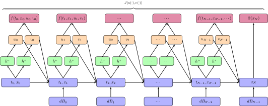
We show the whole network architecture in Figure 1, where husuperscript𝑢h^{u} and hvsuperscript𝑣h^{v} represent respectively the hidden layers of the neural networks φuθusubscriptsuperscript𝜑superscript𝜃𝑢𝑢\varphi^{\theta^{u}}_{u} and φvθvsubscriptsuperscript𝜑superscript𝜃𝑣𝑣\varphi^{\theta^{v}}_{v}. For each of the neural network, the common parameters is used for all the time points, and the time t𝑡t is taken as one of the inputs of the neural network.
Refer to caption
Figure 1: The whole network architecture for case 1: f(t,x,u,v)𝑓𝑡𝑥𝑢𝑣f(t,x,u,v) has an explicit representation. The boxes in purple, green and orange represent respectively the input layer, the hidden layers and the output layers of the neural networks φuθusubscriptsuperscript𝜑superscript𝜃𝑢𝑢\varphi^{\theta^{u}}_{u} and φvθvsubscriptsuperscript𝜑superscript𝜃𝑣𝑣\varphi^{\theta^{v}}_{v}. The data flow of the neural networks is represented with black arrows.

The pseudo-code is shown in Algorithm 1.

Algorithm 1 Numerical algorithm for solving the Hamiltonian system of case 1
1:The Brownian motion ΔBtiΔsubscript𝐵subscript𝑡𝑖\Delta B_{t_{i}}, initial state a𝑎a, and time tisubscript𝑡𝑖t_{i};
2:The output controls utiπsuperscriptsubscript𝑢subscript𝑡𝑖𝜋u_{t_{i}}^{\pi}, vtiπsuperscriptsubscript𝑣subscript𝑡𝑖𝜋v_{t_{i}}^{\pi} and ytiπsuperscriptsubscript𝑦subscript𝑡𝑖𝜋y_{t_{i}}^{\pi}.
3:for  l=0𝑙0l=0 to maxstep𝑚𝑎𝑥𝑠𝑡𝑒𝑝maxstep do
4:     x0l,π,m=asuperscriptsubscript𝑥0𝑙𝜋𝑚𝑎x_{0}^{l,\pi,m}=a, loss=0𝑙𝑜𝑠𝑠0loss=0;
5:     for  i=0𝑖0i=0 to N1𝑁1N-1 do
6:         util,π,m=φu(ti,xtil,π,m;θl);subscriptsuperscript𝑢𝑙𝜋𝑚subscript𝑡𝑖subscript𝜑𝑢subscript𝑡𝑖subscriptsuperscript𝑥𝑙𝜋𝑚subscript𝑡𝑖superscript𝜃𝑙u^{l,\pi,m}_{t_{i}}=\varphi_{u}(t_{i},x^{l,\pi,m}_{t_{i}};\theta^{l});
7:         vtil,π,m=φv(ti,xtil,π,m;θl);subscriptsuperscript𝑣𝑙𝜋𝑚subscript𝑡𝑖subscript𝜑𝑣subscript𝑡𝑖subscriptsuperscript𝑥𝑙𝜋𝑚subscript𝑡𝑖superscript𝜃𝑙v^{l,\pi,m}_{t_{i}}=\varphi_{v}(t_{i},x^{l,\pi,m}_{t_{i}};\theta^{l});
8:         xti+1l,π,m=xtil,π,m+util,π,mΔti+vtil,π,mΔBti;subscriptsuperscript𝑥𝑙𝜋𝑚subscript𝑡𝑖1subscriptsuperscript𝑥𝑙𝜋𝑚subscript𝑡𝑖subscriptsuperscript𝑢𝑙𝜋𝑚subscript𝑡𝑖Δsubscript𝑡𝑖subscriptsuperscript𝑣𝑙𝜋𝑚subscript𝑡𝑖Δsubscript𝐵subscript𝑡𝑖x^{l,\pi,m}_{t_{i+1}}=x^{l,\pi,m}_{t_{i}}+u^{l,\pi,m}_{t_{i}}\Delta t_{i}+v^{l,\pi,m}_{t_{i}}\Delta B_{t_{i}};
9:         loss=loss+f(ti,xtil,π,m,util,π,m,vtil,π,m)Δti;𝑙𝑜𝑠𝑠𝑙𝑜𝑠𝑠𝑓subscript𝑡𝑖superscriptsubscript𝑥subscript𝑡𝑖𝑙𝜋𝑚superscriptsubscript𝑢subscript𝑡𝑖𝑙𝜋𝑚superscriptsubscript𝑣subscript𝑡𝑖𝑙𝜋𝑚Δsubscript𝑡𝑖loss=loss+f(t_{i},x_{t_{i}}^{l,\pi,m},u_{t_{i}}^{l,\pi,m},v_{t_{i}}^{l,\pi,m})\Delta t_{i};
10:     end for
11:     loss=1Mm=1M[loss+Φ(xtNl,π,m);]loss=\dfrac{1}{M}\sum\limits_{m=1}^{M}\left[loss+\Phi(x_{t_{N}}^{l,\pi,m});\right]
12:     θl+1=Adam(θl,loss);superscript𝜃𝑙1𝐴𝑑𝑎𝑚superscript𝜃𝑙𝑙𝑜𝑠𝑠\theta^{l+1}=Adam(\theta^{l},\nabla loss);
13:end for
14:ytiπ=1Mm=1M[j=iN1fx(tj,xtjl,π,m,utjl,π,m,vtjl,π,m)ΔtjΦx(xtNl,π,m)].superscriptsubscript𝑦subscript𝑡𝑖𝜋1𝑀superscriptsubscript𝑚1𝑀delimited-[]superscriptsubscript𝑗𝑖𝑁1subscript𝑓𝑥subscript𝑡𝑗superscriptsubscript𝑥subscript𝑡𝑗𝑙𝜋𝑚superscriptsubscript𝑢subscript𝑡𝑗𝑙𝜋𝑚superscriptsubscript𝑣subscript𝑡𝑗𝑙𝜋𝑚Δsubscript𝑡𝑗subscriptΦ𝑥superscriptsubscript𝑥subscript𝑡𝑁𝑙𝜋𝑚y_{t_{i}}^{\pi}=\dfrac{1}{M}\sum\limits_{m=1}^{M}\Big{[}\sum\limits_{j=i}^{N-1}-f_{x}(t_{j},x_{t_{j}}^{l,\pi,m},u_{t_{j}}^{l,\pi,m},v_{t_{j}}^{l,\pi,m})\Delta t_{j}-\Phi_{x}(x_{t_{N}}^{l,\pi,m})\Big{]}.

3.2 Case 2: the function f(t,x,u,v)𝑓𝑡𝑥𝑢𝑣f(t,x,u,v) does not have an explicit form

For the cases where the function f𝑓f does not have an explicit form, we can still solve the Hamiltonian system (2.3) by constructing a different neural network architecture. For any given optimal triple (x(),u(),v())superscript𝑥superscript𝑢superscript𝑣(x^{*}(\cdot),u^{*}(\cdot),v^{*}(\cdot)) of the optimal control problem (2.7), we assume that the solution (y(),z())superscript𝑦superscript𝑧(y^{*}(\cdot),z^{*}(\cdot)) of (2.22) satisfy

yt=Y(t,xt),zt=Z(t,xt),t[0,T],formulae-sequencesubscriptsuperscript𝑦𝑡𝑌𝑡subscriptsuperscript𝑥𝑡formulae-sequencesubscriptsuperscript𝑧𝑡𝑍𝑡subscriptsuperscript𝑥𝑡for-all𝑡0𝑇y^{*}_{t}=Y(t,x^{*}_{t}),\qquad z^{*}_{t}=Z(t,x^{*}_{t}),\qquad\forall t\in[0,T], (3.7)

for some functions Y𝑌Y and Z𝑍Z. Then according to Proposition 3, we have

J(u(),v())=𝔼[0TF(t,xt,ut,vt,yt,zt)𝑑t+Φ(xT)],𝐽superscript𝑢superscript𝑣𝔼delimited-[]superscriptsubscript0𝑇𝐹𝑡subscriptsuperscript𝑥𝑡subscriptsuperscript𝑢𝑡subscriptsuperscript𝑣𝑡subscriptsuperscript𝑦𝑡subscriptsuperscript𝑧𝑡differential-d𝑡Φsuperscriptsubscript𝑥𝑇J(u^{*}(\cdot),v^{*}(\cdot))=\mathbb{E}\displaystyle\left[\int_{0}^{T}F(t,x^{*}_{t},u^{*}_{t},v^{*}_{t},y^{*}_{t},z^{*}_{t})dt+\Phi(x_{T}^{*})\right], (3.8)

and

dxt=utdt+vtdBt,x0=a,formulae-sequencedsuperscriptsubscript𝑥𝑡subscriptsuperscript𝑢𝑡d𝑡superscriptsubscript𝑣𝑡dsubscript𝐵𝑡superscriptsubscript𝑥0𝑎\mathrm{d}x_{t}^{*}=u^{*}_{t}\mathrm{d}t+v_{t}^{*}\mathrm{d}B_{t},\quad x_{0}^{*}=a, (3.9)

where yt,ztsubscriptsuperscript𝑦𝑡subscriptsuperscript𝑧𝑡y^{*}_{t},z^{*}_{t} satisfy

F(t,xt,ut,vt,yt,zt)=maxy,zF(t,xt,ut,vt,y,z),𝐹𝑡subscriptsuperscript𝑥𝑡subscriptsuperscript𝑢𝑡subscriptsuperscript𝑣𝑡subscriptsuperscript𝑦𝑡subscriptsuperscript𝑧𝑡subscript𝑦𝑧𝐹𝑡subscriptsuperscript𝑥𝑡subscriptsuperscript𝑢𝑡subscriptsuperscript𝑣𝑡𝑦𝑧F(t,x^{*}_{t},u^{*}_{t},v^{*}_{t},y^{*}_{t},z^{*}_{t})=\max\limits_{y,z}F(t,x^{*}_{t},u^{*}_{t},v^{*}_{t},y,z), (3.10)

and F𝐹F is defined by (2.4). Because of the strict concavity and differentiable properties of F𝐹F with respect to y,z𝑦𝑧y,z, the constraint condition (3.10) can be rewritten as

{Fy(t,xt,ut,vt,yt,zt)=0,Fz(t,xt,ut,vt,yt,zt)=0.casessubscript𝐹𝑦𝑡subscriptsuperscript𝑥𝑡subscriptsuperscript𝑢𝑡subscriptsuperscript𝑣𝑡subscriptsuperscript𝑦𝑡subscriptsuperscript𝑧𝑡0otherwisesubscript𝐹𝑧𝑡subscriptsuperscript𝑥𝑡subscriptsuperscript𝑢𝑡subscriptsuperscript𝑣𝑡subscriptsuperscript𝑦𝑡subscriptsuperscript𝑧𝑡0otherwise\begin{cases}F_{y}(t,x^{*}_{t},u^{*}_{t},v^{*}_{t},y^{*}_{t},z^{*}_{t})=0,\vspace{1ex}\\ F_{z}(t,x^{*}_{t},u^{*}_{t},v^{*}_{t},y^{*}_{t},z^{*}_{t})=0.\end{cases} (3.11)

In this way, the Hamiltonian system (2.3) can be solved by solving the stochastic optimal control

J(u(),v())=𝔼[0TF(t,xt,ut,vt,yt,zt)dt+Φ(xT)],𝐽𝑢𝑣𝔼delimited-[]superscriptsubscript0𝑇𝐹𝑡subscript𝑥𝑡subscript𝑢𝑡subscript𝑣𝑡subscript𝑦𝑡subscript𝑧𝑡differential-d𝑡Φsubscript𝑥𝑇J(u(\cdot),v(\cdot))=\mathbb{E}\displaystyle\left[\int_{0}^{T}F(t,x_{t},u_{t},v_{t},y_{t},z_{t})\mathrm{d}t+\Phi(x_{T})\right], (3.12)

with the state constraint

{dxt=utdt+vtdBt,x0=a,Fy(t,xt,ut,vt,yt,zt)=0,Fz(t,xt,ut,vt,yt,zt)=0.casesformulae-sequencedsubscript𝑥𝑡subscript𝑢𝑡d𝑡subscript𝑣𝑡dsubscript𝐵𝑡subscript𝑥0𝑎otherwisesubscript𝐹𝑦𝑡subscript𝑥𝑡subscript𝑢𝑡subscript𝑣𝑡subscript𝑦𝑡subscript𝑧𝑡0otherwisesubscript𝐹𝑧𝑡subscript𝑥𝑡subscript𝑢𝑡subscript𝑣𝑡subscript𝑦𝑡subscript𝑧𝑡0otherwise\begin{cases}\mathrm{d}x_{t}=u_{t}\mathrm{d}t+v_{t}\mathrm{d}B_{t},\quad x_{0}=a,\vspace{1ex}\\ F_{y}(t,x_{t},u_{t},v_{t},y_{t},z_{t})=0,\vspace{1ex}\\ F_{z}(t,x_{t},u_{t},v_{t},y_{t},z_{t})=0.\end{cases} (3.13)

Now we focus on solving (3.12)-(3.13) with a new neural network architecture. Firstly, the Euler-Maruyama scheme (3.1) is used to obtain the discrete form of the optimal control problem. In addition to the neural networks for simulating the controls u𝑢u and v𝑣v, we need to construct two more neural networks for simulating the functions Y𝑌Y and Z𝑍Z,

{y=φyθy(t,x)=φy(t,x;θy)=𝒜yyσy1y𝒜y1yσ1y𝒜1y(t,x)z=φzθz(t,x)=φz(t,x;θz)=𝒜zzσz1z𝒜z1zσ1z𝒜1z(t,x).cases𝑦subscriptsuperscript𝜑superscript𝜃𝑦𝑦𝑡𝑥subscript𝜑𝑦𝑡𝑥superscript𝜃𝑦superscriptsubscript𝒜subscript𝑦𝑦superscriptsubscript𝜎subscript𝑦1𝑦superscriptsubscript𝒜subscript𝑦1𝑦superscriptsubscript𝜎1𝑦superscriptsubscript𝒜1𝑦𝑡𝑥otherwise𝑧subscriptsuperscript𝜑superscript𝜃𝑧𝑧𝑡𝑥subscript𝜑𝑧𝑡𝑥superscript𝜃𝑧superscriptsubscript𝒜subscript𝑧𝑧superscriptsubscript𝜎subscript𝑧1𝑧superscriptsubscript𝒜subscript𝑧1𝑧superscriptsubscript𝜎1𝑧superscriptsubscript𝒜1𝑧𝑡𝑥otherwise\begin{cases}y=\varphi^{\theta^{y}}_{y}(t,x)=\varphi_{y}(t,x;\theta^{y})=\mathcal{A}_{\ell_{y}}^{y}\circ\sigma_{\ell_{y}-1}^{y}\circ\mathcal{A}_{\ell_{y}-1}^{y}\circ\cdots\circ\sigma_{1}^{y}\circ\mathcal{A}_{1}^{y}(t,x)\vspace{1ex}\\ z=\varphi^{\theta^{z}}_{z}(t,x)=\varphi_{z}(t,x;\theta^{z})=\mathcal{A}_{\ell_{z}}^{z}\circ\sigma_{\ell_{z}-1}^{z}\circ\mathcal{A}_{\ell_{z}-1}^{z}\circ\cdots\circ\sigma_{1}^{z}\circ\mathcal{A}_{1}^{z}(t,x).\end{cases} (3.14)

We also use the common parameters on all the time points for each of the four neural networks, and the inputs of each neural network are (t,x)𝑡𝑥(t,x). All of the four neural networks contain one (n+1)𝑛1(n+1)-dim input layer and three (n+10)𝑛10(n+10)-dim hidden layers. The dimensions of the output layer for each neural network are different, that of y𝑦y and u𝑢u are n𝑛n-dim, and that of z𝑧z and v𝑣v are (n×d)𝑛𝑑(n\times d)-dim. We still adopt Adam as the optimizer.

We denote θ=(θuv,θyz)𝜃subscript𝜃𝑢𝑣subscript𝜃𝑦𝑧\theta=(\theta_{uv},\theta_{yz}) as all the parameters of the neural networks, where θuvsubscript𝜃𝑢𝑣\theta_{uv} are the parameters of the neural networks φusubscript𝜑𝑢\varphi_{u} and φvsubscript𝜑𝑣\varphi_{v} (for simulating u𝑢u and v𝑣v), and θyzsubscript𝜃𝑦𝑧\theta_{yz} are the parameters of the neural networks φysubscript𝜑𝑦\varphi_{y} and φzsubscript𝜑𝑧\varphi_{z} (for simulating y𝑦y and z𝑧z).

Then the cost functional of the control problem is approximated by

J(uπ(),vπ())=1Mm=1M[i=0N1F(ti,xtiπ,m,utiπ,m,vtiπ,m,ytiπ,m,ztiπ,m)Δti+Φ(xtNπ,m)],𝐽superscript𝑢𝜋superscript𝑣𝜋1𝑀superscriptsubscript𝑚1𝑀delimited-[]superscriptsubscript𝑖0𝑁1𝐹subscript𝑡𝑖superscriptsubscript𝑥subscript𝑡𝑖𝜋𝑚superscriptsubscript𝑢subscript𝑡𝑖𝜋𝑚superscriptsubscript𝑣subscript𝑡𝑖𝜋𝑚superscriptsubscript𝑦subscript𝑡𝑖𝜋𝑚superscriptsubscript𝑧subscript𝑡𝑖𝜋𝑚Δsubscript𝑡𝑖Φsuperscriptsubscript𝑥subscript𝑡𝑁𝜋𝑚J(u^{\pi}(\cdot),v^{\pi}(\cdot))=\dfrac{1}{M}\sum_{m=1}^{M}\Big{[}\sum_{i=0}^{N-1}F(t_{i},x_{t_{i}}^{\pi,m},u_{t_{i}}^{\pi,m},v_{t_{i}}^{\pi,m},y_{t_{i}}^{\pi,m},z_{t_{i}}^{\pi,m})\Delta t_{i}+\Phi(x_{t_{N}}^{\pi,m})\Big{]}, (3.15)

which is the first loss function we need to minimize, and utiπ,vtiπ,ytiπ,ztiπsuperscriptsubscript𝑢subscript𝑡𝑖𝜋superscriptsubscript𝑣subscript𝑡𝑖𝜋superscriptsubscript𝑦subscript𝑡𝑖𝜋superscriptsubscript𝑧subscript𝑡𝑖𝜋u_{t_{i}}^{\pi},v_{t_{i}}^{\pi},y_{t_{i}}^{\pi},z_{t_{i}}^{\pi} are the outputs of the whole neural networks at time tisubscript𝑡𝑖t_{i}. In addition, in order to guarantee that the conditions (3.11) hold, we introduce the other cost functional

J(yπ(),zπ())𝐽superscript𝑦𝜋superscript𝑧𝜋\displaystyle J(y^{\pi}(\cdot),z^{\pi}(\cdot)) :=1Mm=1Mi=0N1[|Fy(ti,xtiπ,m,utiπ,m,vtiπ,m,ytiπ,m,ztiπ,m)|2\displaystyle:=\dfrac{1}{M}\sum_{m=1}^{M}\sum_{i=0}^{N-1}\Big{[}|F_{y}(t_{i},x_{t_{i}}^{\pi,m},u_{t_{i}}^{\pi,m},v_{t_{i}}^{\pi,m},y_{t_{i}}^{\pi,m},z_{t_{i}}^{\pi,m})|^{2} (3.16)
+|Fz(ti,xtiπ,m,utiπ,m,vtiπ,m,ytiπ,m,ztiπ,m)|2].\displaystyle\qquad\qquad+|F_{z}(t_{i},x_{t_{i}}^{\pi,m},u_{t_{i}}^{\pi,m},v_{t_{i}}^{\pi,m},y_{t_{i}}^{\pi,m},z_{t_{i}}^{\pi,m})|^{2}\Big{]}.

which is at the same time the second loss function we need to minimize in the neural networks.

The update of the neural network parameters is carried out as follows. Suppose that we have finished the update at the iteration step l𝑙l and obtain the parameters θl=(θuvl,θyzl)superscript𝜃𝑙superscriptsubscript𝜃𝑢𝑣𝑙superscriptsubscript𝜃𝑦𝑧𝑙\theta^{l}=(\theta_{uv}^{l},\theta_{yz}^{l}). We first calculate the values (xtiπ,utiπ,vtiπ,ytiπ,ztiπ)subscriptsuperscript𝑥𝜋subscript𝑡𝑖subscriptsuperscript𝑢𝜋subscript𝑡𝑖subscriptsuperscript𝑣𝜋subscript𝑡𝑖subscriptsuperscript𝑦𝜋subscript𝑡𝑖subscriptsuperscript𝑧𝜋subscript𝑡𝑖(x^{\pi}_{t_{i}},u^{\pi}_{t_{i}},v^{\pi}_{t_{i}},y^{\pi}_{t_{i}},z^{\pi}_{t_{i}}) with the parameters θlsuperscript𝜃𝑙\theta^{l}. Then the parameters θuvlsuperscriptsubscript𝜃𝑢𝑣𝑙\theta_{uv}^{l} are updated to θuvl+1superscriptsubscript𝜃𝑢𝑣𝑙1\theta_{uv}^{l+1} by using one step Adam optimization with the first loss function (3.15). In the following, the parameters (θuvl+1,θyzl)superscriptsubscript𝜃𝑢𝑣𝑙1superscriptsubscript𝜃𝑦𝑧𝑙(\theta_{uv}^{l+1},\theta_{yz}^{l}) are used to calculate the values (xtiπ,utiπ,vtiπ,ytiπ,ztiπ)subscriptsuperscript𝑥𝜋subscript𝑡𝑖subscriptsuperscript𝑢𝜋subscript𝑡𝑖subscriptsuperscript𝑣𝜋subscript𝑡𝑖subscriptsuperscript𝑦𝜋subscript𝑡𝑖subscriptsuperscript𝑧𝜋subscript𝑡𝑖(x^{\pi}_{t_{i}},u^{\pi}_{t_{i}},v^{\pi}_{t_{i}},y^{\pi}_{t_{i}},z^{\pi}_{t_{i}}) in (3.16). Then the parameters θyzlsuperscriptsubscript𝜃𝑦𝑧𝑙\theta_{yz}^{l} are updated with the second loss function (3.16) by Adam optimization. In each iteration step, the update of parameters θyzlsuperscriptsubscript𝜃𝑦𝑧𝑙\theta_{yz}^{l} can be performed multiple times, for example κ𝜅\kappa times, to ensure the loss function (3.16) is enough small. And after κ𝜅\kappa times update, the parameters of the neural networks are denoted as θyzl+1superscriptsubscript𝜃𝑦𝑧𝑙1\theta_{yz}^{l+1}. Finally the solution y𝑦y is obtained by taking the conditional expectation of the backward SDE of (2.22) which can be calculated with Monte Carlo simulation:

ytiπ=1Mm=1M[j=iN1Fx(tj,xtjπ,m,utjπ,m,vtjπ,m,ytjπ,m,ztjπ,m)ΔtjΦx(xtNπ,m)].superscriptsubscript𝑦subscript𝑡𝑖𝜋1𝑀superscriptsubscript𝑚1𝑀delimited-[]superscriptsubscript𝑗𝑖𝑁1subscript𝐹𝑥subscript𝑡𝑗superscriptsubscript𝑥subscript𝑡𝑗𝜋𝑚superscriptsubscript𝑢subscript𝑡𝑗𝜋𝑚superscriptsubscript𝑣subscript𝑡𝑗𝜋𝑚superscriptsubscript𝑦subscript𝑡𝑗𝜋𝑚superscriptsubscript𝑧subscript𝑡𝑗𝜋𝑚Δsubscript𝑡𝑗subscriptΦ𝑥superscriptsubscript𝑥subscript𝑡𝑁𝜋𝑚y_{t_{i}}^{\pi}=\dfrac{1}{M}\sum\limits_{m=1}^{M}\Big{[}\sum\limits_{j=i}^{N-1}-F_{x}(t_{j},x_{t_{j}}^{\pi,m},u_{t_{j}}^{\pi,m},v_{t_{j}}^{\pi,m},y_{t_{j}}^{\pi,m},z_{t_{j}}^{\pi,m})\Delta t_{j}-\Phi_{x}(x_{t_{N}}^{\pi,m})\Big{]}. (3.17)

The pseudo-code is given in Algorithm 2.

In fact,we can also deal with the maximum condition (3.10) directly. in this situation, we need to maximize the second objective functional in addition to (3.15),

J(y(),z())=𝔼[0TF(t,xt,ut,vt,yt,zt)]dt.𝐽𝑦𝑧𝔼delimited-[]superscriptsubscript0𝑇𝐹𝑡subscript𝑥𝑡subscript𝑢𝑡subscript𝑣𝑡subscript𝑦𝑡subscript𝑧𝑡d𝑡J(y(\cdot),z(\cdot))=\mathbb{E}\left[\int_{0}^{T}F(t,x_{t},u_{t},v_{t},y_{t},z_{t})\right]\mathrm{d}t. (3.18)

and a similar scheme can be given. The advantage for using the conditions (3.11) instead of (3.18) is that we can determine the influence of the constraint conditions by the value of the cost functional (3.16), as the optimal value of (3.16) should be 0.

4 Numerical results

In this section, we show the numerical results for solving the Hamiltonian system with our proposed algorithms. If not specifically mentioned, we use 6-layer fully connected neural networks for the approximation in these examples, the number of time divisions is set to be N=25𝑁25N=25, and we mainly use a piecewise constant decay learning rate which decreases from 3×1033superscript1033\times 10^{-3} to 1×1031superscript1031\times 10^{-3} with the increase of the number of iteration steps. We adopt ELU as the activation function. In order to show the performance of the proposed algorithms, we compare the results among the two proposed algorithms and the Deep FBSDE method (briefly noted as DFBSDE in the figures and tables of this section) which was developed as Algorithm 1 in our previous work [31]. But different from [31], for better comparison with the novel proposed algorithms, here we use the ELU activation function and remove the batch normalization layer in the Deep FBSDE method. For each algorithm of the examples, we perform ten independent runs to show more accurate results.

Algorithm 2 Numerical algorithm for solving the Hamiltonian system of case 2
1:The Brownian motion ΔBtiΔsubscript𝐵subscript𝑡𝑖\Delta B_{t_{i}}, initial state a𝑎a, and time tisubscript𝑡𝑖t_{i};
2:The processes (xtil,π,util,π,vtil,π,ytil,π,ztil,π)subscriptsuperscript𝑥𝑙𝜋subscript𝑡𝑖subscriptsuperscript𝑢𝑙𝜋subscript𝑡𝑖subscriptsuperscript𝑣𝑙𝜋subscript𝑡𝑖subscriptsuperscript𝑦𝑙𝜋subscript𝑡𝑖subscriptsuperscript𝑧𝑙𝜋subscript𝑡𝑖(x^{l,\pi}_{t_{i}},u^{l,\pi}_{t_{i}},v^{l,\pi}_{t_{i}},y^{l,\pi}_{t_{i}},z^{l,\pi}_{t_{i}}).
3:for  l=0𝑙0l=0 to maxstep𝑚𝑎𝑥𝑠𝑡𝑒𝑝maxstep do
4:     for k=0𝑘0k=0 to κ+1𝜅1\kappa+1 do
5:         x0l,π,m=asuperscriptsubscript𝑥0𝑙𝜋𝑚𝑎x_{0}^{l,\pi,m}=a, loss1=0𝑙𝑜𝑠subscript𝑠10loss_{1}=0, loss2=0𝑙𝑜𝑠subscript𝑠20loss_{2}=0;
6:         for  i=0𝑖0i=0 to N1𝑁1N-1 do
7:              util,π,m=φu(ti,xtil,π,m;θuvl);subscriptsuperscript𝑢𝑙𝜋𝑚subscript𝑡𝑖subscript𝜑𝑢subscript𝑡𝑖subscriptsuperscript𝑥𝑙𝜋𝑚subscript𝑡𝑖superscriptsubscript𝜃𝑢𝑣𝑙u^{l,\pi,m}_{t_{i}}=\varphi_{u}(t_{i},x^{l,\pi,m}_{t_{i}};\theta_{uv}^{l});
8:              vtil,π,m=φv(ti,xtil,π,m;θuvl);subscriptsuperscript𝑣𝑙𝜋𝑚subscript𝑡𝑖subscript𝜑𝑣subscript𝑡𝑖subscriptsuperscript𝑥𝑙𝜋𝑚subscript𝑡𝑖superscriptsubscript𝜃𝑢𝑣𝑙v^{l,\pi,m}_{t_{i}}=\varphi_{v}(t_{i},x^{l,\pi,m}_{t_{i}};\theta_{uv}^{l});
9:              ytil,π,m=φy(ti,xtil,π,m;θyzl);subscriptsuperscript𝑦𝑙𝜋𝑚subscript𝑡𝑖subscript𝜑𝑦subscript𝑡𝑖subscriptsuperscript𝑥𝑙𝜋𝑚subscript𝑡𝑖superscriptsubscript𝜃𝑦𝑧𝑙y^{l,\pi,m}_{t_{i}}=\varphi_{y}(t_{i},x^{l,\pi,m}_{t_{i}};\theta_{yz}^{l});
10:              ztil,π,m=φz(ti,xtil,π,m;θyzl);subscriptsuperscript𝑧𝑙𝜋𝑚subscript𝑡𝑖subscript𝜑𝑧subscript𝑡𝑖subscriptsuperscript𝑥𝑙𝜋𝑚subscript𝑡𝑖superscriptsubscript𝜃𝑦𝑧𝑙z^{l,\pi,m}_{t_{i}}=\varphi_{z}(t_{i},x^{l,\pi,m}_{t_{i}};\theta_{yz}^{l});
11:              xti+1l,π,m=xtil,π,m+util,π,mΔti+vtil,π,mΔBti;subscriptsuperscript𝑥𝑙𝜋𝑚subscript𝑡𝑖1subscriptsuperscript𝑥𝑙𝜋𝑚subscript𝑡𝑖subscriptsuperscript𝑢𝑙𝜋𝑚subscript𝑡𝑖Δsubscript𝑡𝑖subscriptsuperscript𝑣𝑙𝜋𝑚subscript𝑡𝑖Δsubscript𝐵subscript𝑡𝑖x^{l,\pi,m}_{t_{i+1}}=x^{l,\pi,m}_{t_{i}}+u^{l,\pi,m}_{t_{i}}\Delta t_{i}+v^{l,\pi,m}_{t_{i}}\Delta B_{t_{i}};
12:              loss1=loss1+F(ti,xtil,π,m,util,π,m,vtil,π,m,ytil,π,m,ztil,π,m)Δti;𝑙𝑜𝑠subscript𝑠1𝑙𝑜𝑠subscript𝑠1𝐹subscript𝑡𝑖superscriptsubscript𝑥subscript𝑡𝑖𝑙𝜋𝑚superscriptsubscript𝑢subscript𝑡𝑖𝑙𝜋𝑚superscriptsubscript𝑣subscript𝑡𝑖𝑙𝜋𝑚superscriptsubscript𝑦subscript𝑡𝑖𝑙𝜋𝑚superscriptsubscript𝑧subscript𝑡𝑖𝑙𝜋𝑚Δsubscript𝑡𝑖loss_{1}=loss_{1}+F(t_{i},x_{t_{i}}^{l,\pi,m},u_{t_{i}}^{l,\pi,m},v_{t_{i}}^{l,\pi,m},y_{t_{i}}^{l,\pi,m},z_{t_{i}}^{l,\pi,m})\Delta t_{i};
13:              loss2=loss2+1Mm=1M[|Fy(ti,xtil,π,m,util,π,m,vtil,π,m,ytil,π,m,ztil,π,m)|2];𝑙𝑜𝑠subscript𝑠2𝑙𝑜𝑠subscript𝑠21𝑀superscriptsubscript𝑚1𝑀delimited-[]superscriptsubscript𝐹𝑦subscript𝑡𝑖superscriptsubscript𝑥subscript𝑡𝑖𝑙𝜋𝑚superscriptsubscript𝑢subscript𝑡𝑖𝑙𝜋𝑚superscriptsubscript𝑣subscript𝑡𝑖𝑙𝜋𝑚superscriptsubscript𝑦subscript𝑡𝑖𝑙𝜋𝑚superscriptsubscript𝑧subscript𝑡𝑖𝑙𝜋𝑚2loss_{2}=loss_{2}+\dfrac{1}{M}\sum\limits_{m=1}^{M}\left[|F_{y}(t_{i},x_{t_{i}}^{l,\pi,m},u_{t_{i}}^{l,\pi,m},v_{t_{i}}^{l,\pi,m},y_{t_{i}}^{l,\pi,m},z_{t_{i}}^{l,\pi,m})|^{2}\right];
14:              loss2=loss2+1Mm=1M[|Fz(ti,xtil,π,m,util,π,m,vtil,π,m,ytil,π,m,ztil,π,m)|2];𝑙𝑜𝑠subscript𝑠2𝑙𝑜𝑠subscript𝑠21𝑀superscriptsubscript𝑚1𝑀delimited-[]superscriptsubscript𝐹𝑧subscript𝑡𝑖superscriptsubscript𝑥subscript𝑡𝑖𝑙𝜋𝑚superscriptsubscript𝑢subscript𝑡𝑖𝑙𝜋𝑚superscriptsubscript𝑣subscript𝑡𝑖𝑙𝜋𝑚superscriptsubscript𝑦subscript𝑡𝑖𝑙𝜋𝑚superscriptsubscript𝑧subscript𝑡𝑖𝑙𝜋𝑚2loss_{2}=loss_{2}+\dfrac{1}{M}\sum\limits_{m=1}^{M}\left[|F_{z}(t_{i},x_{t_{i}}^{l,\pi,m},u_{t_{i}}^{l,\pi,m},v_{t_{i}}^{l,\pi,m},y_{t_{i}}^{l,\pi,m},z_{t_{i}}^{l,\pi,m})|^{2}\right];
15:         end for
16:         loss1=1Mm=1M[loss1+Φ(xtNl,π,m)];𝑙𝑜𝑠subscript𝑠11𝑀superscriptsubscript𝑚1𝑀delimited-[]𝑙𝑜𝑠subscript𝑠1Φsuperscriptsubscript𝑥subscript𝑡𝑁𝑙𝜋𝑚loss_{1}=\dfrac{1}{M}\sum\limits_{m=1}^{M}\left[loss_{1}+\Phi(x_{t_{N}}^{l,\pi,m})\right];
17:         if k=0𝑘0k=0 then
18:              θuvl=Adam(θuvl,loss1);superscriptsubscript𝜃𝑢𝑣𝑙𝐴𝑑𝑎𝑚superscriptsubscript𝜃𝑢𝑣𝑙𝑙𝑜𝑠subscript𝑠1\theta_{uv}^{l}=Adam(\theta_{uv}^{l},\nabla loss_{1});
19:              θl=(θuvl,θyzl);superscript𝜃𝑙superscriptsubscript𝜃𝑢𝑣𝑙superscriptsubscript𝜃𝑦𝑧𝑙\theta^{l}=(\theta_{uv}^{l},\theta_{yz}^{l});
20:         else
21:              θyzl=Adam(θyzl,loss2);superscriptsubscript𝜃𝑦𝑧𝑙𝐴𝑑𝑎𝑚superscriptsubscript𝜃𝑦𝑧𝑙𝑙𝑜𝑠subscript𝑠2\theta_{yz}^{l}=Adam(\theta_{yz}^{l},\nabla loss_{2});
22:              θl=(θuvl,θyzl);superscript𝜃𝑙superscriptsubscript𝜃𝑢𝑣𝑙superscriptsubscript𝜃𝑦𝑧𝑙\theta^{l}=(\theta_{uv}^{l},\theta_{yz}^{l});
23:         end if
24:     end for
25:     θl+1=(θuvl,θyzl);superscript𝜃𝑙1superscriptsubscript𝜃𝑢𝑣𝑙superscriptsubscript𝜃𝑦𝑧𝑙\theta^{l+1}=(\theta_{uv}^{l},\theta_{yz}^{l});
26:end for
27:ytiπ=1Mm=1M[j=iN1Fx(tj,xtjl,π,m,utjl,π,m,vtjl,π,m,ytjl,π,m,ztjl,π,m)ΔtjΦx(xtNl,π,m)].superscriptsubscript𝑦subscript𝑡𝑖𝜋1𝑀superscriptsubscript𝑚1𝑀delimited-[]superscriptsubscript𝑗𝑖𝑁1subscript𝐹𝑥subscript𝑡𝑗superscriptsubscript𝑥subscript𝑡𝑗𝑙𝜋𝑚superscriptsubscript𝑢subscript𝑡𝑗𝑙𝜋𝑚superscriptsubscript𝑣subscript𝑡𝑗𝑙𝜋𝑚superscriptsubscript𝑦subscript𝑡𝑗𝑙𝜋𝑚superscriptsubscript𝑧subscript𝑡𝑗𝑙𝜋𝑚Δsubscript𝑡𝑗subscriptΦ𝑥superscriptsubscript𝑥subscript𝑡𝑁𝑙𝜋𝑚y_{t_{i}}^{\pi}=\dfrac{1}{M}\sum\limits_{m=1}^{M}\Big{[}\sum\limits_{j=i}^{N-1}-F_{x}(t_{j},x_{t_{j}}^{l,\pi,m},u_{t_{j}}^{l,\pi,m},v_{t_{j}}^{l,\pi,m},y_{t_{j}}^{l,\pi,m},z_{t_{j}}^{l,\pi,m})\Delta t_{j}-\Phi_{x}(x_{t_{N}}^{l,\pi,m})\Big{]}.

4.1 Example 1: a linear Hamiltonian system

Firstly, we consider the following linear quadratic Hamiltonian

H(t,x,y,z)=x,y+14y,y+z,z,Φ(x)=12Qx,x,formulae-sequence𝐻𝑡𝑥𝑦𝑧𝑥𝑦14𝑦𝑦𝑧𝑧Φ𝑥12𝑄𝑥𝑥H(t,x,y,z)=\langle x,y\rangle+\dfrac{1}{4}\langle y,y\rangle+\langle z,z\rangle,\qquad\Phi(x)=\langle\dfrac{1}{2}Qx,x\rangle, (4.1)

where (x,y,z)n+n+n𝑥𝑦𝑧superscript𝑛𝑛𝑛(x,y,z)\in\mathbb{R}^{n+n+n} and Q𝑄Q is a given matrix valued in n×nsuperscript𝑛𝑛\mathbb{R}^{n\times n}, and the corresponding Hamiltonian system is given as

{dxt=(xt+12yt)dt+2ztdBt,dyt=ytdtztdBt,x0=a,yT=Φx(xT)=QxT,casesdsubscript𝑥𝑡subscript𝑥𝑡12subscript𝑦𝑡d𝑡2subscript𝑧𝑡dsubscript𝐵𝑡dsubscript𝑦𝑡subscript𝑦𝑡d𝑡subscript𝑧𝑡dsubscript𝐵𝑡formulae-sequencesubscript𝑥0𝑎subscript𝑦𝑇subscriptΦ𝑥subscript𝑥𝑇𝑄subscript𝑥𝑇\left\{\begin{array}[]{l}\mathrm{d}x_{t}=(x_{t}+\dfrac{1}{2}y_{t})\mathrm{d}t+2z_{t}\mathrm{d}B_{t},\vspace{1ex}\\ -\mathrm{d}y_{t}=y_{t}\mathrm{d}t-z_{t}\mathrm{d}B_{t},\vspace{1ex}\\ x_{0}=a,\qquad y_{T}=-\Phi_{x}(x_{T})=-Qx_{T},\end{array}\right. (4.2)

which is a linear FBSDE and B𝐵B is a 111-dimensional standard Brownian motion. It can be easily check that this linear FBSDE has a unique solution [3, 4, 37].

As is known, the linear FBSDE connects with a Riccati equation. Suppose the solution of FBSDE (4.2) is in the following form:

yt=Ktxt,zt=Mtxt.formulae-sequencesubscript𝑦𝑡subscript𝐾𝑡subscript𝑥𝑡subscript𝑧𝑡subscript𝑀𝑡subscript𝑥𝑡\displaystyle y_{t}=-K_{t}x_{t},\qquad z_{t}=-M_{t}x_{t}.

Combing it with (4.2), we then obtain a Riccati equation

{K˙t12Kt2+2Kt=0,Mt=0,KT=Q,casessubscript˙𝐾𝑡12superscriptsubscript𝐾𝑡22subscript𝐾𝑡0otherwiseformulae-sequencesubscript𝑀𝑡0subscript𝐾𝑇𝑄otherwise\begin{cases}\dot{K}_{t}-\frac{1}{2}K_{t}^{2}+2K_{t}=0,\\ M_{t}=0,\qquad K_{T}=Q,\end{cases} (4.3)

where Ktsubscript𝐾𝑡K_{t} is a matrix function and K˙tsubscript˙𝐾𝑡\dot{K}_{t} is the derivative of Ktsubscript𝐾𝑡K_{t} with respect to t𝑡t. And the solution of (4.3) can be approximated with the ODE45 method in MATLAB (ODE45 in short), which solves determined ordinary differential equations with the four-order Runge-Kutta method. In order to show the performance of our novel proposed algorithms, we take the numerical solution of the Ricatti equation (4.3) with ODE45 as a benchmark.

Now we consider the corresponding optimal control problem,

{dxt=utdt+vtdBt,x0=a,casesdsubscript𝑥𝑡subscript𝑢𝑡d𝑡subscript𝑣𝑡dsubscript𝐵𝑡subscript𝑥0𝑎\left\{\begin{array}[]{l}\mathrm{d}x_{t}=u_{t}\mathrm{d}t+v_{t}\mathrm{d}B_{t},\vspace{1ex}\\ x_{0}=a,\end{array}\right.

with cost functional

J(u(),v())=𝔼{0Tf(t,xt,ut,vt)+Φ(xT)},𝐽𝑢𝑣𝔼superscriptsubscript0𝑇𝑓𝑡subscript𝑥𝑡subscript𝑢𝑡subscript𝑣𝑡Φsubscript𝑥𝑇J(u(\cdot),v(\cdot))=\mathbb{E}\Big{\{}\int_{0}^{T}f(t,x_{t},u_{t},v_{t})+\Phi(x_{T})\Big{\}},

where

f(t,x,u,v)𝑓𝑡𝑥𝑢𝑣\displaystyle f(t,x,u,v) =maxy,zF(t,x,u,v,y,z)absentsubscript𝑦𝑧𝐹𝑡𝑥𝑢𝑣𝑦𝑧\displaystyle=\max_{y,z}F(t,x,u,v,y,z)\vspace{1ex}
=|ux|2+14|v|2,absentsuperscript𝑢𝑥214superscript𝑣2\displaystyle=|u-x|^{2}+\dfrac{1}{4}|v|^{2},

and

F(t,x,u,v,y,z)=y,u+z,vx,y14y,yz,z.𝐹𝑡𝑥𝑢𝑣𝑦𝑧𝑦𝑢𝑧𝑣𝑥𝑦14𝑦𝑦𝑧𝑧F(t,x,u,v,y,z)=\langle y,u\rangle+\langle z,v\rangle-\langle x,y\rangle-\dfrac{1}{4}\langle y,y\rangle-\langle z,z\rangle.

In this example, we set a=(1.0,,1.0)n,T=0.1formulae-sequence𝑎1.01.0superscript𝑛𝑇0.1a=(1.0,\cdots,1.0)\in\mathbb{R}^{n},T=0.1 and give the form of Q𝑄Q as

[1λλλλ1λλλλ1λλλλ1]matrix1𝜆𝜆𝜆𝜆1𝜆𝜆𝜆𝜆1𝜆𝜆𝜆𝜆1\begin{bmatrix}1&\lambda&\lambda&\cdots&\lambda\\ \lambda&1&\lambda&\cdots&\lambda\\ \lambda&\lambda&1&\cdots&\lambda\\ \vdots&\vdots&\vdots&\ddots&\vdots\\ \lambda&\lambda&\lambda&\cdots&1\end{bmatrix}

where λ𝜆\lambda is a given constant between 0 and 1. For example, if λ=0.0𝜆0.0\lambda=0.0, Q=En𝑄subscript𝐸𝑛Q=E_{n} is a n𝑛n-order unit matrix, The numerical result of (4.3) with ODE45 can be solved with K0=1.1573Ensubscript𝐾01.1573subscript𝐸𝑛K_{0}=1.1573E_{n} for n=100𝑛100n=100, then the value of y0subscript𝑦0y_{0} can be obtained by

y0=K0x0=1.1573a.subscript𝑦0subscript𝐾0subscript𝑥01.1573𝑎y_{0}=-K_{0}x_{0}=-1.1573a.

which is taken as the benchmark results in this example.

Even though the function f𝑓f can be solved explicitly in this example, we calculate the numerical results through both the two proposed algorithms and regard that f𝑓f does not have an explicit form in Algorithm 2. The comparison results on the approximated solution y0subscript𝑦0y_{0} between our proposed stochastic control methods (Algorithm 1 and 2) and the Deep FBSDE method are shown in Table 1, and the solution with ODE45 is regarded as the benchmark. Note that when the initial state x=a𝑥𝑎x=a , the solution of y0subscript𝑦0y_{0} is a vector and all its elements are equal, thus we show the value of the first element of y0subscript𝑦0y_{0} in Table 1. Moreover, we show the relative errors between our approximated solution of y0subscript𝑦0y_{0} and that of ODE45, and compute the variances among ten independent runs of the approximated solution y0subscript𝑦0y_{0}. We also change the parameter λ𝜆\lambda, and study the corresponding approximation results.

Table 1: The implementations of different terminal Q𝑄Q with n=100𝑛100n=100
Riccati DEEP FBSDE Alg 1 Alg 2
Mean Rela. Error Var. Mean Rela. Error Var. Mean Rela. Error Var.
λ=0.0𝜆0.0\lambda=0.0 -1.1573 -1.15733 2.907e-05 6.209e-08 -1.15751 1.797e-04 3.141e-07 -1.15651 6.839e-04 3.065e-06
λ=0.2𝜆0.2\lambda=0.2 -11.8093 -11.6314 1.506e-02 2.392e-01 -11.8113 1.733e-04 2.441e-03 -11.8222 1.095e-03 5.997e-03
λ=0.4𝜆0.4\lambda=0.4 -15.2711 -14.1265 7.495e-02 9.101e-01 -15.3120 2.681e-03 1.739e-03 -15.2264 2.930e-03 1.622e-01
λ=0.6𝜆0.6\lambda=0.6 -16.9860 -10.4284 3.861e-01 2.753e+01 -17.0461 3.859e-03 3.563e-03 -17.0516 3.860e-03 4.633e-02
λ=0.8𝜆0.8\lambda=0.8 -18.0101 -9.2087 4.887e-01 2.279e+01 -17.9844 1.426e-03 2.528e-02 -18.1494 7.733e-03 2.726e-02
λ=1.0𝜆1.0\lambda=1.0 -18.6920 -9.9503 4.677e-01 2.300e+01 -18.7162 1.297e-03 2.000e-02 -18.8837 1.026e-02 8.245e-02

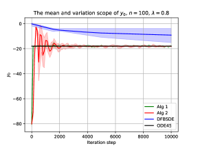
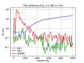
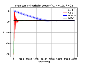
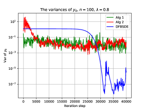
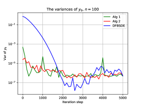
From Table 1, we can see that the novel proposed algorithms show much more stable performance than the Deep FBSDE method. For different terminals with different parameters λ𝜆\lambda, the novel proposed algorithms demonstrate more stable relative errors and variances. The Deep FBSDE method perform well when the terminal is a unit matrix (λ=0.0𝜆0.0\lambda=0.0), but when we change the terminal to other forms (λ0.0𝜆0.0\lambda\not=0.0), the results of the Deep FBSDE method diverge. As we know, the learning rate is one of the important factors affecting the approximation results. When we choose smaller learning rate, the Deep FBSDE method can converge, but it need much more iteration steps than our proposed algorithms. As an example for the case λ0.0𝜆0.0\lambda\not=0.0 with smaller learning rate, we show the approximation results in the following Figure 3 for λ=0.8𝜆0.8\lambda=0.8.

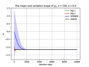
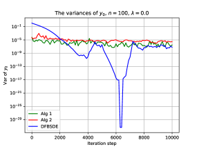
In Figure 2, we show the curves and the variances of the approximated results y0subscript𝑦0y_{0} with different iteration steps for λ=0.0𝜆0.0\lambda=0.0 and λ=0.8𝜆0.8\lambda=0.8 respectively, and the black lines represent the results with ODE45 which is taken as the benchmark. The upper two figures in Figure 2 exhibit the results for λ=0.0𝜆0.0\lambda=0.0. From the upper left figure, we can see that when the number of iteration steps is close to 10000, the approximated solution y0subscript𝑦0y_{0} with Algorithm 1, 2 and the Deep FBSDE method are all very close to the results with ODE45. Moreover, that of Algorithm 1 and 2 have smaller variation scopes among ten independent runs and converge within less iteration steps than that of the Deep FBSDE method. The upper right figure shows that when the number of iteration steps tends to be 10000, the variance curve of y0subscript𝑦0y_{0} with Algorithm 1 and 2 are also close to that of the Deep FBSDE method. The lower two figures in Figure 2 exhibit the results for λ=0.8𝜆0.8\lambda=0.8. We can see that when the number of iteration steps tends to be 10000, the approximation results of Algorithm 1 and 2 are close to the benchmark. However, that of the Deep FBSDE method is far from the benchmark, and the variation scope and variance increase with the increase of iteration steps.
Refer to caption
Refer to caption
Refer to caption
Refer to caption
Figure 2: Approximation results with a piecewise decay learning rate from 3×1033superscript1033\times 10^{-3} to 1×1031superscript1031\times 10^{-3} for λ=0.0𝜆0.0\lambda=0.0 in the upper figures and λ=0.8𝜆0.8\lambda=0.8 in the lower figures. The left figures show the mean and variation scopes of the approximated solution y0subscript𝑦0y_{0} among 10 independent runs, and the right figures exhibit the variance curves of y0subscript𝑦0y_{0} among 10 independent runs. The black lines in the left figure represent the results with ODE45 which are taken as the benchmarks. We can see that our novel proposed algorithms(Algorithms 1 and 2) have more stable convergence and converge within less iteration steps.
Refer to caption
Refer to caption
Figure 3: Approximation results with a constant learning rate of 1×1031superscript1031\times 10^{-3}. We can see from the left figure that comparing with the novel proposed algorithms(Algorithms 1 and 2), the Deep FBSDE method needs more iteration steps to achieve stable convergence, and it has a much smaller variance at the end of the training from the right figure.

4.2 Example 2: a nonlinear Hamiltonian system

Given the Hamiltonian H𝐻H as

H(t,x,y,z)=12y,ycos2x+12z,zsin2x+y,cosx+z,sinx12x,x𝐻𝑡𝑥𝑦𝑧12𝑦𝑦superscript2𝑥12𝑧𝑧superscript2𝑥𝑦𝑥𝑧𝑥12𝑥𝑥H(t,x,y,z)=\dfrac{1}{2}\langle y,y\circ\cos^{2}x\rangle+\dfrac{1}{2}\langle z,z\circ\sin^{2}x\rangle+\langle y,\cos x\rangle+\langle z,\sin x\rangle-\dfrac{1}{2}\langle x,x\rangle (4.4)

and

Φ(x)=12x,x,Φ𝑥12𝑥𝑥\Phi(x)=\dfrac{1}{2}\langle x,x\rangle, (4.5)

where (x,y,z)n+n+n𝑥𝑦𝑧superscript𝑛𝑛𝑛(x,y,z)\in\mathbb{R}^{n+n+n}. Here \circ represents the Hadamard product,

xy=(x1y1,x2y2,,xnyn)n,x,ynformulae-sequence𝑥𝑦subscript𝑥1subscript𝑦1subscript𝑥2subscript𝑦2subscript𝑥𝑛subscript𝑦𝑛superscript𝑛for-all𝑥𝑦superscript𝑛x\circ y=(x_{1}y_{1},x_{2}y_{2},\cdots,x_{n}y_{n})\in\mathbb{R}^{n},\qquad\forall x,y\in\mathbb{R}^{n}

The corresponding Hamiltonian system is

{dxt=cosxt(ytcosxt+1)dt+sinxt(ztsinxt+1)dBt,dyt=[ytsinxt(ytcosxt+1)+ztcosxt(ztsinxt+1)xt]dtztdBt,x0=a,yT=Φx(xT),casesdsubscript𝑥𝑡subscript𝑥𝑡subscript𝑦𝑡subscript𝑥𝑡1d𝑡subscript𝑥𝑡subscript𝑧𝑡subscript𝑥𝑡1dsubscript𝐵𝑡dsubscript𝑦𝑡delimited-[]subscript𝑦𝑡subscript𝑥𝑡subscript𝑦𝑡subscript𝑥𝑡1subscript𝑧𝑡subscript𝑥𝑡subscript𝑧𝑡subscript𝑥𝑡1subscript𝑥𝑡d𝑡subscript𝑧𝑡dsubscript𝐵𝑡formulae-sequencesubscript𝑥0𝑎subscript𝑦𝑇subscriptΦ𝑥subscript𝑥𝑇\left\{\begin{array}[]{l}\mathrm{d}x_{t}=\cos x_{t}\circ(y_{t}\circ\cos x_{t}+1)\mathrm{d}t+\sin x_{t}\circ(z_{t}\circ\sin x_{t}+1)\circ\mathrm{d}B_{t},\vspace{1ex}\\ -\mathrm{d}y_{t}=\Big{[}-y_{t}\circ\sin x_{t}\circ(y_{t}\circ\cos x_{t}+1)+z_{t}\circ\cos x_{t}\circ(z_{t}\circ\sin x_{t}+1)-x_{t}\Big{]}\mathrm{d}t\\ \qquad\qquad-z_{t}\circ\mathrm{d}B_{t},\vspace{1ex}\\ x_{0}=a,\qquad y_{T}=-\Phi_{x}(x_{T}),\end{array}\right. (4.6)

where B𝐵B is a n𝑛n-dimensional Brownian motion.

Here we introduce a stochastic optimal control problem which is different from (2.6):

{dxt=cosxt(ut+1)dt+sinxt(vt+1)dBtx0=a,casesdsubscript𝑥𝑡subscript𝑥𝑡subscript𝑢𝑡1d𝑡subscript𝑥𝑡subscript𝑣𝑡1dsubscript𝐵𝑡subscript𝑥0𝑎\left\{\begin{array}[]{l}\mathrm{d}x_{t}=\cos x_{t}\circ(u_{t}+1)\mathrm{d}t+\sin x_{t}\circ(v_{t}+1)\circ\mathrm{d}B_{t}\vspace{1ex}\\ x_{0}=a,\end{array}\right. (4.7)

with the cost functional

J(u(),v())=𝔼{0Tf(t,xt,ut,vt)𝑑t+Φ(xT)},𝐽𝑢𝑣𝔼superscriptsubscript0𝑇𝑓𝑡subscript𝑥𝑡subscript𝑢𝑡subscript𝑣𝑡differential-d𝑡Φsubscript𝑥𝑇J(u(\cdot),v(\cdot))=\mathbb{E}\left\{\int_{0}^{T}f(t,x_{t},u_{t},v_{t})dt+\Phi(x_{T})\right\},

where f(t,x,u,v)𝑓𝑡𝑥𝑢𝑣f(t,x,u,v) is given as

f(t,x,u,v)𝑓𝑡𝑥𝑢𝑣\displaystyle f(t,x,u,v) =maxy,zF(t,x,u,v,y,z)absentsubscript𝑦𝑧𝐹𝑡𝑥𝑢𝑣𝑦𝑧\displaystyle=\max_{y,z}F(t,x,u,v,y,z)\vspace{1ex}
=maxy,z{y,cosx(u+1)+z,sinx(v+1)H(t,x,y,z)}.absentsubscript𝑦𝑧𝑦𝑥𝑢1𝑧𝑥𝑣1𝐻𝑡𝑥𝑦𝑧\displaystyle=\max_{y,z}\left\{\langle y,\cos x\circ(u+1)\rangle+\langle z,\sin x\circ(v+1)\rangle-H(t,x,y,z)\right\}.

Then f(t,x,u,v)𝑓𝑡𝑥𝑢𝑣f(t,x,u,v) can be solved as

f(t,x,u,v)=12[x,x+u,u+v,v],𝑓𝑡𝑥𝑢𝑣12delimited-[]𝑥𝑥𝑢𝑢𝑣𝑣f(t,x,u,v)=\dfrac{1}{2}\big{[}\langle x,x\rangle+\langle u,u\rangle+\langle v,v\rangle\big{]},

and

y𝑦\displaystyle y =u1cosx,absent𝑢1𝑥\displaystyle=u\circ\dfrac{1}{\cos x},
z𝑧\displaystyle z =v1sinx.absent𝑣1𝑥\displaystyle=v\circ\dfrac{1}{\sin x}.

Define h(t,x,y,v,y,z)𝑡𝑥𝑦𝑣𝑦𝑧h(t,x,y,v,y,z) as

h(t,x,u,v,y,z)=y,cosx(u+1)+z,sinx(v+1)f(t,x,u,v),𝑡𝑥𝑢𝑣𝑦𝑧𝑦𝑥𝑢1𝑧𝑥𝑣1𝑓𝑡𝑥𝑢𝑣\displaystyle h(t,x,u,v,y,z)=\langle y,\cos x\circ(u+1)\rangle+\langle z,\sin x\circ(v+1)\rangle-f(t,x,u,v),

then we get the value of y0subscript𝑦0y_{0} by

y0subscript𝑦0\displaystyle y_{0} =𝔼{0Thx(t,xt,ut,vt,yt,zt)𝑑tΦx(xT)}absent𝔼superscriptsubscript0𝑇subscript𝑥𝑡subscript𝑥𝑡subscript𝑢𝑡subscript𝑣𝑡subscript𝑦𝑡subscript𝑧𝑡differential-d𝑡subscriptΦ𝑥subscript𝑥𝑇\displaystyle=\mathbb{E}\left\{\int_{0}^{T}h_{x}(t,x_{t},u_{t},v_{t},y_{t},z_{t})dt-\Phi_{x}(x_{T})\right\}
=𝔼{0T(uttanxt(ut+1)+vtcotxt(vt+1)xt)Φx(xT)}.absent𝔼superscriptsubscript0𝑇subscript𝑢𝑡subscript𝑥𝑡subscript𝑢𝑡1subscript𝑣𝑡subscript𝑥𝑡subscript𝑣𝑡1subscript𝑥𝑡subscriptΦ𝑥subscript𝑥𝑇\displaystyle=\mathbb{E}\left\{\int_{0}^{T}(-u_{t}\circ\tan x_{t}\circ(u_{t}+1)+v_{t}\circ\cot x_{t}\circ(v_{t}+1)-x_{t})-\Phi_{x}(x_{T})\right\}.

We set a=(1.0,,1.0)n𝑎1.01.0superscript𝑛a=(1.0,\cdots,1.0)\in\mathbb{R}^{n} and T=0.1𝑇0.1T=0.1. The comparison results among Algorithm 1, Algorithm 2 and the Deep FBSDE method are shown in Figure 4. We can see from the left figure that when the number of iteration steps is 5000, The approximated value of Y0subscript𝑌0Y_{0} with Algorithm 1 and the Deep FBSDE method are very close, which are 1.08351.0835-1.0835 and 1.08341.0834-1.0834, respectively. And the approximated solution with Algorithm 2 is 1.12081.1208-1.1208, which is slightly smaller than that with Algorithm 1 and the Deep FBSDE method. Similar to the first example, the variation scope of y0subscript𝑦0y_{0} for Algorithm 1, 2 are much smaller than that of the Deep FBSDE method. Besides, at the end of the training, the variances of y0subscript𝑦0y_{0} for Algorithm 1, 2 and the Deep FBSDE method are very close.
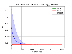
Refer to caption
Refer to caption
Figure 4: We can see from the figure that when the number of iteration steps tends to be 5000, the approximated values of y0subscript𝑦0y_{0} for all the three methods are close. However, the Deep FBSDE method shows larger variation scopes than Algorithm 1 and 2 during the training. And the variances of these three methods are also close at the end of the training.

4.3 Example 3: a Hamiltonian system with exponents in the drift term

In the third example, we solve a Hamiltonian system with exponents in the drift term. Consider the following Hamiltonian

H(t,x,y,z)=log(i=1nexp(yi))+12y,y+z,z+z,x+15x,x,𝐻𝑡𝑥𝑦𝑧superscriptsubscript𝑖1𝑛subscript𝑦𝑖12𝑦𝑦𝑧𝑧𝑧𝑥15𝑥𝑥H(t,x,y,z)=\log\left(\sum_{i=1}^{n}\exp(y_{i})\right)+\dfrac{1}{2}\langle y,y\rangle+\langle z,z\rangle+\langle z,x\rangle+\dfrac{1}{5}\langle x,x\rangle, (4.8)

where (x,y,z)n+n+n𝑥𝑦𝑧superscript𝑛𝑛𝑛(x,y,z)\in\mathbb{R}^{n+n+n} and y=(y1,,yn)𝑦subscript𝑦1subscript𝑦𝑛y=(y_{1},\cdots,y_{n}). The terminal function is given as Φ(x)=12x,xΦ𝑥12𝑥𝑥\Phi(x)=\dfrac{1}{2}\langle x,x\rangle. Then the Hamiltonian system we need to solve is given as following,

{dxt=[exp(yt)(i=1nexp(yit))1+yt]dt+(xt+2zt)dBt,dyt=(25xt+zt)dtztdBt,x0=a,yT=Φx(xT),casesdsubscript𝑥𝑡delimited-[]subscript𝑦𝑡superscriptsuperscriptsubscript𝑖1𝑛subscript𝑦𝑖𝑡1subscript𝑦𝑡d𝑡subscript𝑥𝑡2subscript𝑧𝑡dsubscript𝐵𝑡dsubscript𝑦𝑡25subscript𝑥𝑡subscript𝑧𝑡d𝑡subscript𝑧𝑡dsubscript𝐵𝑡formulae-sequencesubscript𝑥0𝑎subscript𝑦𝑇subscriptΦ𝑥subscript𝑥𝑇\left\{\begin{array}[]{l}\mathrm{d}x_{t}=\left[\exp(y_{t})\left(\sum_{i=1}^{n}\exp(y_{it})\right)^{-1}+y_{t}\right]\mathrm{d}t+(x_{t}+2z_{t})\circ\mathrm{d}B_{t},\vspace{1ex}\\ -\mathrm{d}y_{t}=(\dfrac{2}{5}x_{t}+z_{t})\mathrm{d}t-z_{t}\circ\mathrm{d}B_{t},\vspace{1ex}\\ x_{0}=a,\qquad y_{T}=-\Phi_{x}(x_{T}),\end{array}\right. (4.9)

where exp(yt)=(exp(yit),,exp(ynt))subscript𝑦𝑡subscript𝑦𝑖𝑡subscript𝑦𝑛𝑡\exp(y_{t})=(\exp(y_{it}),\cdots,\exp(y_{nt})) and B𝐵B is a n𝑛n-dimensional Brownian motion.

The corresponding stochastic optimal control problem is

{dxt=utdt+vtdBt,x0=a,casesdsubscript𝑥𝑡subscript𝑢𝑡d𝑡subscript𝑣𝑡dsubscript𝐵𝑡otherwisesubscript𝑥0𝑎otherwise\begin{cases}\mathrm{d}x_{t}=u_{t}\mathrm{d}t+v_{t}\circ\mathrm{d}B_{t},\vspace{1ex}\\ x_{0}=a,\end{cases}

with the cost functional

J(u(),v())=𝔼{0Tf(t,xt,ut,vt)dt+Φ(xT)},𝐽𝑢𝑣𝔼superscriptsubscript0𝑇𝑓𝑡subscript𝑥𝑡subscript𝑢𝑡subscript𝑣𝑡differential-d𝑡Φsubscript𝑥𝑇\displaystyle J(u(\cdot),v(\cdot))=\mathbb{E}\left\{\int_{0}^{T}f(t,x_{t},u_{t},v_{t})\mathrm{d}t+\Phi(x_{T})\right\},

where

f(t,x,u,v)𝑓𝑡𝑥𝑢𝑣\displaystyle f(t,x,u,v) =maxy,zF(t,x,u,v,y,z),absentsubscript𝑦𝑧𝐹𝑡𝑥𝑢𝑣𝑦𝑧\displaystyle=\max_{y,z}F(t,x,u,v,y,z), (4.10)
=maxy,z{y,u+z,vH(t,x,y,z)}.absentsubscript𝑦𝑧𝑦𝑢𝑧𝑣𝐻𝑡𝑥𝑦𝑧\displaystyle=\max_{y,z}\left\{\langle y,u\rangle+\langle z,v\rangle-H(t,x,y,z)\right\}.

Different from the previous two examples, in this example, the function f𝑓f defined as (4.10) does not have an explicit representation. In this situation, Algorithm 1 is not applicable, thus we mainly make the comparison between the results of Algorithm 2 and the Deep FBSDE method.

We set T=0.2𝑇0.2T=0.2, a=(0.5,,0.5)n𝑎0.50.5superscript𝑛a=(0.5,\cdots,0.5)\in\mathbb{R}^{n} and n=100𝑛100n=100 in this example. The comparison results between Algorithm 2 and the Deep FBSDE method are shown in Figure 5. We can see that at the end of the training, the approximated solution y0subscript𝑦0y_{0} of the two methods are close, and both the variances are small enough. Similar with the previous two examples, Algorithm 2 shows smaller variation scope and converges within less iteration steps than the Deep FBSDE method.
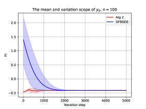
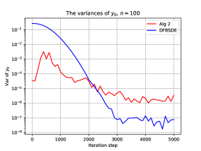
Refer to caption
Refer to caption
Figure 5: We can see from the above figure that at the end of training, the approximated solutions of y0subscript𝑦0y_{0} with both Algorithm 2 and the Deep FBSDE method are very close, and the mean values of y0subscript𝑦0y_{0} among 10 independent runs are 0.412970.41297-0.41297 for Algorithm 2 and 0.412110.41211-0.41211 for the Deep FBSDE method. The variance of Algorithm 2 is slightly larger than that of the Deep FBSDE method, but it converges within less iteration steps.

In the implementations of Algorithm 2 for all the three examples, we minimize the norm of the derivatives of the function F𝐹F with respect to y𝑦y and z𝑧z according to (3.16) so that they are equal to 00. As an alternative, we can also maximize the cost functional defined as (3.18) in the implementations.

5 Conclusion

In this paper, different from the general way of solving the FBSDEs, we propose a novel method which solve the Hamiltonian system from the view of the stochastic optimal control via deep learning. Two different algorithms suitable for different cases are developed. From the numerical results, the novel proposed Algorithms 1 and 2 demonstrate faster convergence rate and more stable performance than the Deep FBSDE method. In some cases, Algorithm 1 and 2 shows higher accuracy.

References

  • [1] R. Ortega, A. J. Van Der Schaft, I. Mareels, and B. Maschke, “Putting energy back in control,” IEEE Control Systems Magazine, vol. 21, no. 2, pp. 18–33, 2001.
  • [2] R. Ortega, A. van der Schaft, B. Maschke, and G. Escobar, “Interconnection and damping assignment passivity-based control of port-controlled hamiltonian systems,” Automatica, vol. 38, no. 4, pp. 585–596, 2002.
  • [3] Y. Hu and S. Peng, “Solution of forward-backward stochastic differential equations,” Probability Theory and Related Fields, vol. 103, no. 2, pp. 273–283, 1995.
  • [4] S. Peng and Z. Wu, “Fully coupled forward-backward stochastic differential equations and applications to optimal control,” Siam Journal on Control and Optimization, vol. 37, no. 3, pp. 825–843, 1999.
  • [5] S. Peng, “Problem of eigenvalues of stochastic hamiltonian systems with boundary conditions,” Stochastic Processes and Their Applications, vol. 88, no. 2, pp. 259–290, 2000.
  • [6] Y. Hu and J. Yong, “Forward–backward stochastic differential equations with nonsmooth coefficients,” Stochastic Processes and their Applications, vol. 87, no. 1, pp. 93–106, 2000.
  • [7] J. Ma, P. Protter, and J. Yong, “Solving forward-backward stochastic differential equations explicitly — a four step scheme,” Probability Theory and Related Fields, vol. 98, no. 3, pp. 339–359, 1994.
  • [8] J. Ma and J. Yong, “Solvability of forward-backward sdes and the nodal set of hamilton-jacobi-bellman equations,” Chinese Annals of Mathematics, 1993.
  • [9] J. Ma and J. Yong, “Approximate solvability of forward—backward stochastic differential equations,” Applied Mathematics and Optimization, vol. 45, no. 1, pp. 1–22, 2002.
  • [10] N. E. Karoui, S. Peng, and M. C. Quenez, “Backward Stochastic Differential Equations in Finance,” Mathematical Finance, vol. 7, no. 1, pp. 1–71, 1997. _eprint: https://onlinelibrary.wiley.com/doi/pdf/10.1111/1467-9965.00022.
  • [11] E. Pardoux and S. Tang, “Forward-backward stochastic differential equations and quasilinear parabolic PDEs,” Probability Theory and Related Fields, vol. 114, pp. 123–150, may 1999.
  • [12] A. Bensoussan, “Lectures on stochastic control,” in Nonlinear filtering and stochastic control, pp. 1–62, Springer, 1982.
  • [13] J. Yong and X. Zhou, Stochastic Controls-Hamiltonian System and HJB Equations. Springer, 1999.
  • [14] E. Tadmor, “A review of numerical methods for nonlinear partial differential equations,” Bulletin of the American Mathematical Society, vol. 49, no. 4, pp. 507–554, 2012.
  • [15] B. Bouchard and N. Touzi, “Discrete-time approximation and monte-carlo simulation of backward stochastic differential equations,” Stochastic Processes & Their Applications, vol. 111, no. 2, pp. 175–206, 2004.
  • [16] V. Bally and G. Pages, “A quantization algorithm for solving multidimensional discrete-time optimal stopping problems,” Bernoulli, vol. 9, no. 6, pp. 1003–1049, 2003.
  • [17] M. A. Jin, S. Jie, and Y. Zhao, “On numerical approximations of forward-backward stochastic differential equations,” Siam Journal on Numerical Analysis, vol. 46, no. 5, pp. 2636–2661, 2008.
  • [18] C. Bender and J. Zhang, “Time discretization and markovian iteration for coupled fbsdes,” Annals of Applied Probability, vol. 18, no. 1, pp. 143–177, 2008.
  • [19] F. Yu, W. Zhao, and T. Zhou, “Multistep schemes for forward backward stochastic differential equations with jumps,” Journal of Scientific Computing, vol. 69, no. 2, pp. 1–22, 2016.
  • [20] E. Weinan, M. Hutzenthaler, A. Jentzen, and T. Kruse, “On multilevel picard numerical approximations for high-dimensional nonlinear parabolic partial differential equations and high-dimensional nonlinear backward stochastic differential equations,” arXiv: Numerical Analysis, 2017.
  • [21] G. N. Milstein and M. V. Tretyakov, “Numerical algorithms for forward-backward stochastic differential equations connected with semilinear parabolic equations,” vol. 28, pp. 561–582, 2004.
  • [22] F. Yu, W. Zhao, and Z. Tao, “Efficient spectral sparse grid approximations for solving multi-dimensional forward backward sdes,” Discrete and Continuous Dynamical Systems - Series B, vol. 22, no. 9, 2016.
  • [23] T. P. Huijskens, M. Ruijter, and C. W. Oosterlee, “Efficient numerical fourier methods for coupled forward-backward sdes,” Journal of Computational and Applied Mathematics, vol. 296, pp. 593–612, 2016.
  • [24] E. Weinan, J. Han, and A. Jentzen, “Deep learning-based numerical methods for high-dimensional parabolic partial differential equations and backward stochastic differential equations,” Communications in Mathematics & Statistics, vol. 5, no. 4, pp. 349–380, 2017.
  • [25] J. Han, A. Jentzen, and E. Weinan, “Solving high-dimensional partial differential equations using deep learning,” Proceedings of the National Academy of Sciences of the United States of America, vol. 115, no. 34, pp. 8505–8510, 2018.
  • [26] C. Huré, H. Pham, and X. Warin, “Deep backward schemes for high-dimensional nonlinear PDEs,” arXiv:1902.01599 [cs, math, stat], June 2020.
  • [27] H. Pham, X. Warin, and M. Germain, “Neural networks-based backward scheme for fully nonlinear PDEs,” SN Partial Differential Equations and Applications, vol. 2, p. 16, Feb. 2021.
  • [28] M. Raissi, “Forward-backward stochastic neural networks: Deep learning of high-dimensional partial differential equations,” arXiv: 1804.07010, 2018.
  • [29] H. Wang, H. Chen, A. Sudjianto, R. Liu, and Q. Shen, “Deep learning-based bsde solver for libor market model with application to bermudan swaption pricing and hedging,” 2018.
  • [30] J. Han and J. Long, “Convergence of the deep bsde method for coupled fbsdes,” arXiv:1811.01165, 2018.
  • [31] S. Ji, S. Peng, Y. Peng, and X. Zhang, “Three algorithms for solving high-dimensional fully coupled fbsdes through deep learning,” IEEE Intelligent Systems, vol. 35, no. 3, pp. 71–84, 2020.
  • [32] R. T. ROCKAFELLAR, Convex Analysis. Princeton University Press, 1970.
  • [33] G. Cybenko, “Approximation by superpositions of a sigmoidal function,” Mathematics of Control, Signals and Systems, vol. 2, no. 4, pp. 303–314, 1989.
  • [34] K. Hornik, “Approximation capabilities of multilayer feedforward networks,” Neural Networks, vol. 4, no. 2, pp. 251–257, 1991.
  • [35] J. Han and W. E, “Deep learning approximation for stochastic control problems,” NIPS Workshop on Deep Reinforcement Learning, 2016.
  • [36] A. C. Wilson, R. Roelofs, R. Stern, N. Srebro, and B. Recht, “The marginal value of adaptive gradient methods in machine learning,” 31st Conference on Neural Information Processing Systems (NIPS 2017), 2017.
  • [37] J. Ma, Z. Wu, D. Zhang, and J. Zhang, “On well-posedness of forward-backward SDEs–A unified approach,” The Annals of Applied Probability, vol. 25, no. 4, pp. 2168 – 2214, 2015.