Asymptotic-Preserving Neural Networks for Multiscale Time-Dependent Linear Transport Equations

Shi Jin School of Mathematical Sciences, Shanghai Jiao Tong University, Shanghai, 200240, P. R. China. Institute of Natural Sciences, MOE-LSC, Shanghai Jiao Tong University, Shanghai, 200240, P. R. China. Zheng Ma School of Mathematical Sciences, Shanghai Jiao Tong University, Shanghai, 200240, P. R. China. Institute of Natural Sciences, MOE-LSC, Shanghai Jiao Tong University, Shanghai, 200240, P. R. China. Qing Yuan Research Institute, Shanghai Jiao Tong University, Shanghai, 200240, China Keke Wu School of Mathematical Sciences, Shanghai Jiao Tong University, Shanghai, 200240, P. R. China.
Abstract

In this paper we develop a neural network for the numerical simulation of time-dependent linear transport equations with diffusive scaling and uncertainties. The goal of the network is to resolve the computational challenges of curse-of-dimensionality and multiple scales of the problem. We first show that a standard Physics-Informed Neural Network (PINN) fails to capture the multiscale nature of the problem, hence justifies the need to use Asymptotic-Preserving Neural Networks (APNNs). We show that not all classical AP formulations are fit for the neural network approach. We construct a micro-macro decomposition based neural network, and also build in a mass conservation mechanism into the loss function, in order to capture the dynamic and multiscale nature of the solutions. Numerical examples are used to demonstrate the effectiveness of this APNNs.

1 Introduction

In the category of multiscale modeling, kinetic equations are bridges between continuum and atomistic models [1]. There are two major challenges in kinetic modeling. First is the curse-of-dimensionality, since kinetic equations describe the evolution of probability density function of large number of particles, thus are defined in the phase space, typically a six-dimensional problem plus time. When uncertainties are considered the dimension can be much higher [2, 3, 4, 5, 6]. Another difficulty is the multiscale nature. Kinetic equations usually contain small or multiple space and/or temporal scales, characterized by the Knudsen number, which is the dimensionless mean free path or time. Often multiscale computations involve the coupling of models at different scales by different numerical schemes [7]. When the Knudsen number is small, kinetic equations can often be approximated by macroscopic hydrodynamic or diffusion equations [8]. In this regime, numerical simulations become prohibitively expensive, since one needs to numerically resolve the small physical scales. Asymptotic-preserving (AP) schemes are those that mimic the asymptotic transitions from the kinetic or hyperbolic equations to their macroscopic (hydrodynamic or diffusive) limits in discrete setting  [9]. Since the mid-1990’s, the development of AP schemes for such problems has generated many interests  [9, 10, 11]. The AP strategy has been proved to be a powerful and robust technique to address multiscale problems in many kinetic and hyperbolic problems. The main advantage of AP schemes is that they are very efficient in the hydrodynamic or diffusive regime, since they do not need to resolve the small physical parameters numerically and yet can still capture the macroscopic behavior governed by the hydrodynamic or diffusion equations. In fact, carefully constructed AP schemes avoid the difficulty of coupling a microscopic solver with a macroscopic one, as the micro solver automatically becomes a macro solver in the zero Knudsen number limit. It was proved, in the case of linear transport with a diffusive scaling, the AP scheme converges uniformly with respect to the scaling parameter [12].

Due to aforementioned computational challenges of kinetic modeling and computations, efficient computational methods that can efficiently deal with both curse-of-dimensionality and multiple scales are highly desirable. Classical tools to address such issues often use Monte-Carlo methods, which have low-order accuracy, and become exceedingly expensive when the Knudsen number becomes small [13, 14, 15]. In this paper we seek a machine learning based method to tackle these challenges.

The idea of using machine learning method, especially with deep neural networks (DNNs) to solve high-dimensional PDEs has been developed rapidly and achieved some success recently in many problems [16, 17, 18, 19]. In all these approaches, the DNNs came down to minimize the loss function, a high dimensional non-convex optimization problem. The choices of losses usually make a difference for the PDEs; see [16, 17, 19, 20, 21, 22, 23, 24, 25] for reviews and references therein. For applications in kinetic type equations see [26, 27, 28, 29, 30]. The machine learning/DNNs approach has several advantages. First, it could deal with high-dimensional PDEs due to the strong capacity/representativeness of DNNs. Second, it is a mesh-free method so it can deal with problems in complex domain and geometry. Third, it is user friendly to implement for equations by treating the residual error of PDEs as loss function. One does not need to construct numerical schemes carefully for approximate derivatives through automatic differentiation technique.

However, the DNN approach also brings some drawbacks compared with classical numerical methods. The two well-known drawbacks are: lack of high accuracy and long training time due to large number of parameters in DNNs and the use of stochastic gradient method during the training step for high-dimensional non-convex functions [31]. Most importantly, as we find in this article, that the standard DeepRitz, PINNs, or NeuralOp approaches have difficulties in dealing with multiscales, especially for the unsteady problems. This is the main issue we want to address in this paper, and our main strategy to tackle the multiscale challenges is to design an Asymptotic-Preserving neural networks (APNNs).

In this paper, we present a framework of APNNs methods for linear transport equations that could exhibit diffusive behavior. The idea is based on the following observations when using PINNs-like framework to solve multiscale PDEs:

  1. 1.

    For the time-dependent/unsteady PDEs, PINNs converts it to a minimization problem of the population/empirical risk/loss in the least square formulation [17], which can only capture the leading order/single scale–depending on how to design the loss– behavior. This is not only due to poor selection of the risk/loss and commonly used first-order gradient based optimization algorithms, but also due to the underlying Frequency-principle [32] of DNN fitting function that is difficult to capture the small scale (high frequency) part of the solutions.

  2. 2.

    Unlike traditional AP schemes, the PINNs framework ignores the asymptotic property of the problem thus cannot capture the macroscopic behavior-which correspond to small physical parameters– efficiently or effectively. On the contrary, our strategy is to define the loss based on an AP strategy, which captures the correct asymptotic behavior when the physical scaling parameters become small, namely the loss has the AP property.

  3. 3.

    Beyong the AP property, in addition, the conservation or other physical constraints needed to be satisfied by the DNN solutions to get the correct solutions when dealing with small scaling parameters. We propose such a conservation mechanism in our loss.

We first define the APNNs:

Definition 1.

Assume the solution is parameterized using DNN in certain way and trained by using a gradient-based method to minimize a Loss/Risk. Then we say it is APNN if, as the physical scaling parameter tends to zero, the loss of the microscopic equation converges to the loss of the macroscopic equation. That is, the loss when viewed as a numerical approximation of the original equation, has the AP property.

Our main contributions lie in the following aspects:

  1. 1.

    We propose the concept of Asymptotic-preserving neural networks (APNNs) which is a class of machine learning methods that can solve efficiently multiscale equations whose scaling parameter may differ in several orders of magnitude. By requiring loss to satisfy certain conditions (including AP and conservation), these methods can solve the equations accurately, efficiently and use number of neurons and layers independent of the scaling parameter. Moreover, it can automatically capture the limiting macroscopic behavior as the scaling parameter tends to zero.

  2. 2.

    A novel deep neural network with structure is constructed for the linear transport equations that exhibit multiscale or diffusive behavior. By using the micro-macro decomposition formulation in the loss and building in the mass-conservation structure, we obtain a machine learning approach to solve the equation which is APNN.

This paper is organized as follows. In Section 2, a brief introduction of the linear transport equation and its diffusion limit is given. The AP micro-macro decomposition is presented in Section 3. Section 4 is our main part where APNNs is introduced with a detailed illustration. Specially, the loss function we choose is based on the micro-macro decomposition and we present our deep neural network that preserves both the asymptotic diffusion limit as well as mass conservation. Numerical problems for both multiscale and high-dimensional uncertainties are given in Section 5, which are solved by APNNs and compared with PINNs. The paper is concluded in Section 6.

2 The transport equation and its diffusion limit

Consider the multidimensional transport equation with the diffusive scaling. Let f(t,𝒙,𝒗)𝑓𝑡𝒙𝒗f(t,\bm{x},\bm{v}) be the density distribution for particles at space point 𝒙𝒟d𝒙𝒟superscript𝑑\bm{x}\in\mathcal{D}\subset\mathbb{R}^{d}, time t[0,T]:=𝒯𝑡0𝑇assign𝒯t\in[0,T]:=\mathcal{T}\subset\mathbb{R}, and traveling in direction 𝒗Ωd𝒗Ωsuperscript𝑑\bm{v}\in\Omega\subset\mathbb{R}^{d}, with Ωd𝒗=SsubscriptΩdifferential-d𝒗𝑆\int_{\Omega}\mathop{}\!\mathrm{d}\bm{v}=S. Here ΩΩ\Omega is symmetric in 𝒗𝒗\bm{v}, meaning that Ωg(𝒗)d𝒗=0subscriptΩ𝑔𝒗differential-d𝒗0\int_{\Omega}g(\bm{v})\,\mathop{}\!\mathrm{d}\bm{v}=0 for any function g𝑔g odd in 𝒗𝒗\bm{v}. Then f𝑓f solves the linear transport equation

εtf+𝒗xf=1εf+εQ,𝜀subscript𝑡𝑓𝒗subscript𝑥𝑓1𝜀𝑓𝜀𝑄\varepsilon\partial_{t}f+\bm{v}\cdot\nabla_{x}f=\frac{1}{\varepsilon}\mathcal{L}f+\varepsilon Q, (1)

with the collision operator

f=σSSΩfd𝒗σf,𝑓subscript𝜎𝑆𝑆subscriptΩ𝑓differential-dsuperscript𝒗𝜎𝑓\mathcal{L}f=\frac{\sigma_{S}}{S}\int_{\Omega}f\,\mathop{}\!\mathrm{d}{\bm{v}^{\prime}}-\sigma f, (2)

where σ=σ(𝒙)𝜎𝜎𝒙\sigma=\sigma(\bm{x}) is the total transport coefficient, σS=σS(𝒙)subscript𝜎𝑆subscript𝜎𝑆𝒙\sigma_{S}=\sigma_{S}(\bm{x}) is the scattering coefficient, Q=Q(𝒙)𝑄𝑄𝒙Q=Q(\bm{x}) is the source term, ε>0𝜀0\varepsilon>0 is the dimensionless mean free path (Knudsen number). Notice the time variable has been rescaled to the long-time scale O(1/ε)𝑂1𝜀O(1/\varepsilon). Here,

σS=σε2σA,subscript𝜎𝑆𝜎superscript𝜀2subscript𝜎𝐴\sigma_{S}=\sigma-\varepsilon^{2}\sigma_{A}, (3)

where σA=σA(𝒙)subscript𝜎𝐴subscript𝜎𝐴𝒙\sigma_{A}=\sigma_{A}(\bm{x}) is the absorption coefficient. Such an equation arises in neutron transport, radiative transfer [33], wave propagation in random media [34], etc. In all these applications, the scaling gives rise to a diffusion equation as ε0𝜀0\varepsilon\to 0 [35], which is

tρ=D𝒙(1σ𝒙ρ)σAρ+Q,subscript𝑡𝜌𝐷subscript𝒙1𝜎subscript𝒙𝜌subscript𝜎𝐴𝜌𝑄\partial_{t}\rho=D\nabla_{\bm{x}}\cdot\left(\frac{1}{\sigma}\nabla_{\bm{x}}\rho\right)-\sigma_{A}\rho+Q\,, (4)

where ρ=Ωf(𝒗)d𝒗𝜌subscriptΩ𝑓𝒗differential-d𝒗\rho=\int_{\Omega}f(\bm{v})\,\mathop{}\!\mathrm{d}\bm{v}. For different collision operators, the diffusion coefficient D𝐷D may be different. For examples, D=1/3𝐷13D=1/3 in one-dimensional slab geometry and D=1/2𝐷12D=1/2 when ΩΩ\Omega is a unit sphere in two dimension. This diffusion approximation can be obtained by using the Hilbert expansion with the ansatz

f=f(0)+εf(1)+ε2f(2)+𝑓superscript𝑓0𝜀superscript𝑓1superscript𝜀2superscript𝑓2f=f^{(0)}+\varepsilon f^{(1)}+\varepsilon^{2}f^{(2)}+\cdots (5)

and balance the terms by the order in ε𝜀\varepsilon. The diffusion approximation can also be derived using the so-called even- and odd-parities [36], or micro-macro decomposition technique [37] and various Asymptotic-preserving schemes can be constructed based on these methods [9].

For example in the 111-d case, by splitting equation (1) and define even- and odd-parities as

r(t,x,v)𝑟𝑡𝑥𝑣\displaystyle r(t,x,v) =12[f(t,x,v)+f(t,x,v)],absent12delimited-[]𝑓𝑡𝑥𝑣𝑓𝑡𝑥𝑣\displaystyle=\frac{1}{2}[f(t,x,v)+f(t,x,-v)], (6)
j(t,x,v)𝑗𝑡𝑥𝑣\displaystyle j(t,x,v) =12ε[f(t,x,v)f(t,x,v)],absent12𝜀delimited-[]𝑓𝑡𝑥𝑣𝑓𝑡𝑥𝑣\displaystyle=\frac{1}{2\varepsilon}[f(t,x,v)-f(t,x,-v)],

one can obtain

tr+vxj=σSε2(ρr)σAr+Q,subscript𝑡𝑟𝑣subscript𝑥𝑗subscript𝜎𝑆superscript𝜀2𝜌𝑟subscript𝜎𝐴𝑟𝑄\displaystyle\partial_{t}r+v\partial_{x}j=\frac{\sigma_{S}}{\varepsilon^{2}}(\rho-r)-\sigma_{A}r+Q, (7)
tj+vε2xr=σSε2jσAj.subscript𝑡𝑗𝑣superscript𝜀2subscript𝑥𝑟subscript𝜎𝑆superscript𝜀2𝑗subscript𝜎𝐴𝑗\displaystyle\partial_{t}j+\frac{v}{\varepsilon^{2}}\partial_{x}r=-\frac{\sigma_{S}}{\varepsilon^{2}}j-\sigma_{A}j.

As ε0𝜀0\varepsilon\to 0, the first equation gives r=ρ𝑟𝜌r=\rho and the second gives vxr=σSj𝑣subscript𝑥𝑟subscript𝜎𝑆𝑗v\partial_{x}r=-\sigma_{S}j. Substituting back to the first equation will result

tρ=v2x(1σSxρ)σAρ+Q,subscript𝑡𝜌superscript𝑣2subscript𝑥1subscript𝜎𝑆subscript𝑥𝜌subscript𝜎𝐴𝜌𝑄\partial_{t}\rho=-v^{2}\partial_{x}(\frac{1}{\sigma_{S}}\partial_{x}\rho)-\sigma_{A}\rho+Q, (8)

which after integrating over v𝑣v yields to the diffusion limit equation (4).

One thing we would like to mention here is that not all classical AP formulations, based on which AP schemes have been constructed, can be used to construct the correct APNN method with the desired AP property. See Remark 3. This is an interesting phenomenon we want to emphasis in this paper. As will be seen in the sequel, the micro-macro decomposition based formulation will help us to construct the desired APNN.

3 The micro-macro decomposition

In this section we describe the problem setup and then introduce the micro-macro decomposition. Consider the linear transport equation with initial and boundary conditions over a bounded domain 𝒯×𝒟×Ω𝒯𝒟Ω\mathcal{T}\times\mathcal{D}\times\Omega:

{εtf+𝒗xf=1εf+εQ,(t,𝒙,𝒗)𝒯×𝒟×Ω,f=FB,(t,𝒙,𝒗)𝒯×𝒟×Ω,f=f0,(t,𝒙,𝒗){t=0}×𝒟×Ω,cases𝜀subscript𝑡𝑓𝒗subscript𝑥𝑓1𝜀𝑓𝜀𝑄𝑡𝒙𝒗𝒯𝒟Ω𝑓subscript𝐹B𝑡𝒙𝒗𝒯𝒟Ω𝑓subscript𝑓0𝑡𝒙𝒗𝑡0𝒟Ω\left\{\begin{array}[]{ll}\varepsilon\partial_{t}f+\bm{v}\cdot\nabla_{x}f=\frac{1}{\varepsilon}\mathcal{L}f+\varepsilon Q,&(t,\bm{x},\bm{v})\in\mathcal{T}\times\mathcal{D}\times\Omega,\\ \mathcal{B}f=F_{\text{B}},&(t,\bm{x},\bm{v})\in\mathcal{T}\times\partial\mathcal{D}\times\Omega,\\ \mathcal{I}f=f_{0},&(t,\bm{x},\bm{v})\in\{t=0\}\times\mathcal{D}\times\Omega,\end{array}\right. (9)

where FB,f0subscript𝐹Bsubscript𝑓0F_{\text{B}},f_{0} are given functions; 𝒟𝒟\partial\mathcal{D} is the boundary of 𝒟𝒟\mathcal{D}, and ,\mathcal{B},\mathcal{I} are boundary and initial operators, respectively. More precisely we consider the 111-d and 222-d cases in this paper.

One-dimensional case

Consider the one-dimensional transport equation in slab geometry

εtf+vxf=1ε(σS211fdvσf)+εQ,xL<x<xR,1v1,formulae-sequenceformulae-sequence𝜀subscript𝑡𝑓𝑣subscript𝑥𝑓1𝜀subscript𝜎𝑆2superscriptsubscript11𝑓differential-dsuperscript𝑣𝜎𝑓𝜀𝑄subscript𝑥𝐿𝑥subscript𝑥𝑅1𝑣1\varepsilon\partial_{t}f+v\partial_{x}f=\frac{1}{\varepsilon}\left(\frac{\sigma_{S}}{2}\int_{-1}^{1}f\,\mathop{}\!\mathrm{d}v^{\prime}-\sigma f\right)+\varepsilon Q,\quad x_{L}<x<x_{R},\quad-1\leq v\leq 1, (10)

with in-flow boundary conditions as,

f(t,xL,v)𝑓𝑡subscript𝑥𝐿𝑣\displaystyle f(t,x_{L},v) =FL(v)forv>0,formulae-sequenceabsentsubscript𝐹𝐿𝑣for𝑣0\displaystyle=F_{L}(v)\quad\text{for}\quad v>0, (11)
f(t,xR,v)𝑓𝑡subscript𝑥𝑅𝑣\displaystyle f(t,x_{R},v) =FR(v)forv<0,formulae-sequenceabsentsubscript𝐹𝑅𝑣for𝑣0\displaystyle=F_{R}(v)\quad\text{for}\quad v<0,

or periodic boundary condition

f(t,xL,v)=f(t,xR,v).𝑓𝑡subscript𝑥𝐿𝑣𝑓𝑡subscript𝑥𝑅𝑣f(t,x_{L},v)=f(t,x_{R},v). (12)

The initial function is given as a function of x𝑥x and v𝑣v

f(0,x,v)=f0(x,v).𝑓0𝑥𝑣subscript𝑓0𝑥𝑣f(0,x,v)=f_{0}(x,v). (13)

Two-dimensional case

The two-dimensional case is very similar except the velocity/angular variables are constrained in the unit circle

εtf+𝒗𝒙f=1ε(σS2π|𝒗|=1fd𝒗σf)+εQ,𝒙Γ2,|𝒗|=1,formulae-sequenceformulae-sequence𝜀subscript𝑡𝑓𝒗subscript𝒙𝑓1𝜀subscript𝜎𝑆2𝜋subscript𝒗1𝑓differential-dsuperscript𝒗𝜎𝑓𝜀𝑄𝒙Γsuperscript2𝒗1\varepsilon\partial_{t}f+\bm{v}\cdot\partial_{\bm{x}}f=\frac{1}{\varepsilon}\left(\frac{\sigma_{S}}{2\pi}\int_{|\bm{v}|=1}f\,\mathop{}\!\mathrm{d}\bm{v}^{\prime}-\sigma f\right)+\varepsilon Q,\quad\bm{x}\in\Gamma\subset\mathbb{R}^{2},\quad|\bm{v}|=1, (14)

with 𝒗=(ξ,η),1ξ,η1,ξ2+η2=1formulae-sequence𝒗𝜉𝜂formulae-sequencemuch-less-than1𝜉formulae-sequencemuch-less-than𝜂1superscript𝜉2superscript𝜂21\bm{v}=(\xi,\eta),-1\ll\xi,\eta\ll 1,\xi^{2}+\eta^{2}=1. The in-flow boundary condition is,

f(t,𝒙,𝒗)=FB(𝒙,𝒗)for𝒏𝒗<0,𝒙Γ,formulae-sequence𝑓𝑡𝒙𝒗subscript𝐹𝐵𝒙𝒗forformulae-sequence𝒏𝒗0𝒙Γf(t,\bm{x},\bm{v})=F_{B}(\bm{x},\bm{v})\quad\text{for}\quad\bm{n}\cdot\bm{v}<0,\quad\bm{x}\in\partial\Gamma, (15)

where 𝒏𝒏\bm{n} is the outer normal of the boundary. The initial condition is

f(0,𝒙,𝒗)=f0(𝒙,𝒗).𝑓0𝒙𝒗subscript𝑓0𝒙𝒗f(0,\bm{x},\bm{v})=f_{0}(\bm{x},\bm{v}). (16)

In this section, we describe the micro-macro decomposition formulation for the linear transport equation. It is a useful mechanism to build AP schemes [37]. The idea begins with the decomposition of f𝑓f into the equilibrium part ρ𝜌\rho and the non-equilibrium part g𝑔g:

f=ρ+εg,𝑓𝜌𝜀𝑔f=\rho+\varepsilon g, (17)

where

ρ=1SΩfd𝒗.𝜌1𝑆subscriptΩ𝑓differential-dsuperscript𝒗\rho=\frac{1}{S}\int_{\Omega}f\,\mathop{}\!\mathrm{d}{\bm{v}^{\prime}}. (18)

The non-equilibrium part g𝑔g clearly satisfies g=0delimited-⟨⟩𝑔0\left\langle g\right\rangle=0, where

g:=1SΩgd𝒗=0.assigndelimited-⟨⟩𝑔1𝑆subscriptΩ𝑔differential-dsuperscript𝒗0\left\langle g\right\rangle:=\frac{1}{S}\int_{\Omega}g\,\mathop{}\!\mathrm{d}{\bm{v}^{\prime}}=0. (19)

Applying equation (17) in (1) gives

εtρ+ε2tg+𝒗𝒙ρ+ε𝒗𝒙g=g+εQ.𝜀subscript𝑡𝜌superscript𝜀2subscript𝑡𝑔𝒗subscript𝒙𝜌𝜀𝒗subscript𝒙𝑔𝑔𝜀𝑄\varepsilon\partial_{t}\rho+\varepsilon^{2}\partial_{t}g+\bm{v}\cdot\nabla_{\bm{x}}\rho+\varepsilon\bm{v}\cdot\nabla_{\bm{x}}g=\mathcal{L}g+\varepsilon Q. (20)

Integrating this equation with respect to v𝑣v one obtains the following continuity equation:

tρ+𝒙𝒗g=Q.subscript𝑡𝜌subscript𝒙delimited-⟨⟩𝒗𝑔𝑄\partial_{t}\rho+\nabla_{\bm{x}}\cdot\left\langle\bm{v}g\right\rangle=Q. (21)

Define operator Π:Π()(𝒗)=:ΠΠ𝒗delimited-⟨⟩\Pi:\Pi(\cdot)(\bm{v})=\left\langle\cdot\right\rangle and I𝐼I is the identity operator. Then an evolution equation on g𝑔g is found by applying the orthogonal projection IΠ𝐼ΠI-\Pi to equation (20):

ε2tg+ε(IΠ)(𝒗𝒙g)+𝒗𝒙ρ=g+(IΠ)εQ.superscript𝜀2subscript𝑡𝑔𝜀𝐼Π𝒗subscript𝒙𝑔𝒗subscript𝒙𝜌𝑔𝐼Π𝜀𝑄\varepsilon^{2}\partial_{t}g+\varepsilon(I-\Pi)(\bm{v}\cdot\nabla_{\bm{x}}g)+\bm{v}\cdot\nabla_{\bm{x}}\rho=\mathcal{L}g+(I-\Pi)\varepsilon Q. (22)

Finally, (21) and (22) together with the constraint (18) and (19) constitute the micro-macro formulation of (1):

{tρ+𝒙𝒗g=Q,ε2tg+ε(IΠ)(𝒗𝒙g)+𝒗𝒙ρ=g+(IΠ)εQ,g=0.\left\{\begin{aligned} &\partial_{t}\rho+\nabla_{\bm{x}}\cdot\left\langle{\bm{v}}g\right\rangle=Q,\\ &\varepsilon^{2}\partial_{t}g+\varepsilon(I-\Pi)(\bm{v}\cdot\nabla_{\bm{x}}g)+\bm{v}\cdot\nabla_{\bm{x}}\rho=\mathcal{L}g+(I-\Pi)\varepsilon Q,\\ &\langle g\rangle=0.\end{aligned}\right. (23)

or the last equation can be replaced by enforcing it only at initial time

{tρ+𝒙𝒗g=Q,ε2tg+ε(IΠ)(𝒗𝒙g)+𝒗𝒙ρ=g+(IΠ)εQ,g(0,x)=0.\left\{\begin{aligned} &\partial_{t}\rho+\nabla_{\bm{x}}\cdot\left\langle{\bm{v}}g\right\rangle=Q,\\ &\varepsilon^{2}\partial_{t}g+\varepsilon(I-\Pi)(\bm{v}\cdot\nabla_{\bm{x}}g)+\bm{v}\cdot\nabla_{\bm{x}}\rho=\mathcal{L}g+(I-\Pi)\varepsilon Q,\\ &\langle g\rangle(0,x)=0.\end{aligned}\right. (24)

This is due to the conservation of gdelimited-⟨⟩𝑔\langle g\rangle with respect to t𝑡t and can be seen easily by integrating the second equation with respect to v𝑣v,

tg=0.subscript𝑡delimited-⟨⟩𝑔0\partial_{t}\langle g\rangle=0. (25)

When ε0𝜀0\varepsilon\to 0, the above system formally approaches

{tρ+𝒙𝒗g=Q,𝒗𝒙ρ=g.casessubscript𝑡𝜌subscript𝒙delimited-⟨⟩𝒗𝑔𝑄missing-subexpression𝒗subscript𝒙𝜌𝑔missing-subexpression\left\{\begin{array}[]{ll}\partial_{t}\rho+\nabla_{\bm{x}}\cdot\left\langle{\bm{v}}g\right\rangle=Q,\\ \bm{v}\cdot\nabla_{\bm{x}}\rho=\mathcal{L}g.\end{array}\right. (26)

The second equation yields

g=1(𝒗𝒙ρ),𝑔superscript1𝒗subscript𝒙𝜌g=\mathcal{L}^{-1}(\bm{v}\cdot\nabla_{\bm{x}}\rho), (27)

which, when plugging into the first equation and integrating over v𝑣v, gives the diffusion equation (4).

Remark 1.

In (23) or (24) we singled out the condition g=0delimited-⟨⟩𝑔0\langle g\rangle=0. This is not necessary in constructing classical AP schemes [37]. However, for DNN this condition is usually not automatically satisfied and one needs to impose this condition in the loss, as shown in the next section.

4 Asymptotic-Preserving Neural Networks

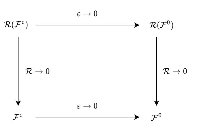
Unlike classical numerical schemes, DNN framework consists of three ingredients: a neural network parametrization of the solution, a population and empirical loss/risk and an optimization algorithm. In terms of proposed APNNs, the key component is to design a loss that has the AP property. The diagram in Fig. 1 illustrates the idea of APNNs.
Refer to caption
Figure 1: Illustration of APNNs. εsuperscript𝜀\mathcal{F^{\varepsilon}} is the microscopic equation that depends on the small scale parameter ε𝜀\varepsilon and 0superscript0\mathcal{F}^{0} is its macroscopic limit as ε0𝜀0\varepsilon\to 0, which is independent of ε𝜀\varepsilon. The latent solution of εsuperscript𝜀\mathcal{F^{\varepsilon}} is approximated by neural networks with its measure denoted by (ε)superscript𝜀\mathcal{R}(\mathcal{F^{\varepsilon}}). The asymptotic limit of (ε)superscript𝜀\mathcal{R}(\mathcal{F^{\varepsilon}}) as ε0𝜀0\varepsilon\to 0, if exists, is denoted by (0)superscript0\mathcal{R}(\mathcal{F}^{0}). If loss(0)𝑙𝑜𝑠𝑠superscript0loss(\mathcal{F}^{0}) is a good measure of 0superscript0\mathcal{F}^{0}, then it is called asymptotic-preserving (AP).

The procedure of a deep neural network for solving a PDE problem consists of three parts: a neural network structure, a loss, and a method to minimize loss over the parameter space.

In what follows, conventional notations for deep neural networks (DNNs)111BAAI.2020. Suggested Notation for Machine Learning. https://github.com/mazhengcn/suggested-notation-for-machine-learning. are introduced. An L𝐿L-layer feed forward neural network is defined recursively as,

fθ[0](x)superscriptsubscript𝑓𝜃delimited-[]0𝑥\displaystyle f_{\theta}^{[0]}(x) =x,absent𝑥\displaystyle=x, (28)
fθ[l](x)superscriptsubscript𝑓𝜃delimited-[]𝑙𝑥\displaystyle f_{\theta}^{[l]}(x) =σ(W[l1]fθ[l1](x)+b[l1]), 1lL1,formulae-sequenceabsent𝜎superscript𝑊delimited-[]𝑙1superscriptsubscript𝑓𝜃delimited-[]𝑙1𝑥superscript𝑏delimited-[]𝑙11𝑙𝐿1\displaystyle=\sigma\circ(W^{[l-1]}f_{\theta}^{[l-1]}(x)+b^{[l-1]}),\,1\leq l\leq L-1,
fθ(x)subscript𝑓𝜃𝑥\displaystyle f_{\theta}(x) =fθ[L](x)=W[L1]fθ[L1](x)+b[L1],absentsuperscriptsubscript𝑓𝜃delimited-[]𝐿𝑥superscript𝑊delimited-[]𝐿1superscriptsubscript𝑓𝜃delimited-[]𝐿1𝑥superscript𝑏delimited-[]𝐿1\displaystyle=f_{\theta}^{[L]}(x)=W^{[L-1]}f_{\theta}^{[L-1]}(x)+b^{[L-1]},

where W[l]ml+1×ml,blml+1,m0=din=dformulae-sequencesuperscript𝑊delimited-[]𝑙superscriptsubscript𝑚𝑙1subscript𝑚𝑙formulae-sequencesuperscript𝑏𝑙superscriptsubscript𝑚𝑙1subscript𝑚0subscript𝑑𝑖𝑛𝑑W^{[l]}\in\mathbb{R}^{m_{l+1}\times m_{l}},b^{l}\in\mathbb{R}^{m_{l+1}},m_{0}=d_{in}=d is the input dimension, mL=d0subscript𝑚𝐿subscript𝑑0m_{L}=d_{0} is the output dimension, σ𝜎\sigma is a scalar function and """""\circ" means entry-wise operation. We denote the set of parameters by θ𝜃\theta. For simplicity of neural network presentation, we denote the layers by a list, i.e., [m0,,mL]subscript𝑚0subscript𝑚𝐿[m_{0},\cdots,m_{L}].

There are various choices to build the loss, when applying a DNN to solve a given PDE. In this paper we compare several results about different scale of ε𝜀\varepsilon in equation (9) with Physics-informed Neural Networks (PINNs) and our proposed Asymptotic Preserving Neural Networks (APNNs). PINNs has the loss as the mean-square error or the residual associated to the given PDE. In contrast, APNNs rewrites the original PDE into a system in asymptotic-preserving form and takes their mean-square residual error as the loss. Boundary and initial conditions are treated as a regularization or penalty term with penalty parameters λ1,λ2subscript𝜆1subscript𝜆2\lambda_{1},\lambda_{2} into the loss, which are selected for better performance.

For simplicity in the following discussion we set σ=σS=1𝜎subscript𝜎𝑆1\sigma=\sigma_{S}=1.

4.1 The failure of PINNs to resolve small scales

For PINNs, one neural network is applied to directly approximate the density function f(t,x,v)𝑓𝑡𝑥𝑣f(t,x,v),

NNθ(t,𝒙,𝒗)f(t,𝒙,𝒗).subscriptNN𝜃𝑡𝒙𝒗𝑓𝑡𝒙𝒗\text{NN}_{\theta}(t,\bm{x},\bm{v})\approx f(t,\bm{x},\bm{v}). (29)

The inputs of DNN are (t,𝒙,𝒗)𝑡𝒙𝒗(t,\bm{x},\bm{v}), i.e., m0=3,5subscript𝑚035m_{0}=3,5 for 111-d and 222-d respectively. The output is a scalar which represents the value of f𝑓f at (t,𝒙,𝒗)𝑡𝒙𝒗(t,\bm{x},\bm{v}). Since f𝑓f is always non-negative, we put an exponential function at the last output layer of the DNN. To be precise, we use

fθNN(t,𝒙,𝒗):=exp(f~θNN(t,𝒙,𝒗))f(t,𝒙,𝒗)assignsubscriptsuperscript𝑓NN𝜃𝑡𝒙𝒗subscriptsuperscript~𝑓NN𝜃𝑡𝒙𝒗𝑓𝑡𝒙𝒗f^{\text{NN}}_{\theta}(t,\bm{x},\bm{v}):=\exp\left(-\tilde{f}^{\text{NN}}_{\theta}(t,\bm{x},\bm{v})\right)\approx f(t,\bm{x},\bm{v}) (30)

to represent the numerical solution of f𝑓f. Then the least square of the residual of the original transport equation (1) is used as the target loss function, together with boundary and initial conditions as penalty terms, that is,

PINNε=subscriptsuperscript𝜀PINNabsent\displaystyle\mathcal{R}^{\varepsilon}_{\text{PINN}}= 1|𝒯×𝒟×Ω|𝒯𝒟Ω|ε2tfθNN+ε𝒗xfθNNfθNNε2Q|2d𝒗d𝒙dt1𝒯𝒟Ωsubscript𝒯subscript𝒟subscriptΩsuperscriptsuperscript𝜀2subscript𝑡subscriptsuperscript𝑓NN𝜃𝜀𝒗subscript𝑥subscriptsuperscript𝑓NN𝜃subscriptsuperscript𝑓NN𝜃superscript𝜀2𝑄2differential-d𝒗differential-d𝒙differential-d𝑡\displaystyle\frac{1}{|\mathcal{T}\times\mathcal{D}\times\Omega|}\int_{\mathcal{T}}\int_{\mathcal{D}}\int_{\Omega}\left|\varepsilon^{2}\partial_{t}f^{\text{NN}}_{\theta}+\varepsilon\bm{v}\cdot\nabla_{x}f^{\text{NN}}_{\theta}-\mathcal{L}f^{\text{NN}}_{\theta}-\varepsilon^{2}Q\right|^{2}\mathop{}\!\mathrm{d}{\bm{v}}\mathop{}\!\mathrm{d}{\bm{x}}\mathop{}\!\mathrm{d}{t} (31)
+λ1|𝒯×𝒟×Ω|𝒯𝒟Ω|fθNNFB|2d𝒗d𝒙dtsubscript𝜆1𝒯𝒟Ωsubscript𝒯subscript𝒟subscriptΩsuperscriptsubscriptsuperscript𝑓NN𝜃subscript𝐹B2differential-d𝒗differential-d𝒙differential-d𝑡\displaystyle+\frac{\lambda_{1}}{|\mathcal{T}\times\partial\mathcal{D}\times\Omega|}\int_{\mathcal{T}}\int_{\partial\mathcal{D}}\int_{\Omega}|\mathcal{B}f^{\text{NN}}_{\theta}-F_{\text{B}}|^{2}\mathop{}\!\mathrm{d}{\bm{v}}\mathop{}\!\mathrm{d}{\bm{x}}\mathop{}\!\mathrm{d}{t}
+λ2|𝒟×Ω|𝒟Ω|fθNNf0|2d𝒗d𝒙,subscript𝜆2𝒟Ωsubscript𝒟subscriptΩsuperscriptsubscriptsuperscript𝑓NN𝜃subscript𝑓02differential-d𝒗differential-d𝒙\displaystyle+\frac{\lambda_{2}}{|\mathcal{D}\times\Omega|}\int_{\mathcal{D}}\int_{\Omega}|\mathcal{I}f^{\text{NN}}_{\theta}-f_{0}|^{2}\mathop{}\!\mathrm{d}{\bm{v}}\mathop{}\!\mathrm{d}{\bm{x}},

where λ1subscript𝜆1\lambda_{1} and λ2subscript𝜆2\lambda_{2} are the penalty weights to be tuned. Then a standard stochastic gradient method (SGD) or Adam optimizer is used to find the global minimum of this loss. Notice that in order to approximate each integral in the loss we use randomly sampled batch at every step, to be detailed in section 5.

Now let us check whether this PINN method is AP. We only need to focus on the first term of (31)

PINN, residualε:=1|𝒯×𝒟×Ω|𝒯𝒟Ω|ε2tfθNN+ε𝒗xfθNNfθNNε2Q|2d𝒗d𝒙dt.assignsubscriptsuperscript𝜀PINN, residual1𝒯𝒟Ωsubscript𝒯subscript𝒟subscriptΩsuperscriptsuperscript𝜀2subscript𝑡subscriptsuperscript𝑓NN𝜃𝜀𝒗subscript𝑥subscriptsuperscript𝑓NN𝜃subscriptsuperscript𝑓NN𝜃superscript𝜀2𝑄2differential-d𝒗differential-d𝒙differential-d𝑡\mathcal{R}^{\varepsilon}_{\text{PINN, residual}}:=\frac{1}{|\mathcal{T}\times\mathcal{D}\times\Omega|}\int_{\mathcal{T}}\int_{\mathcal{D}}\int_{\Omega}\left|\varepsilon^{2}\partial_{t}f^{\text{NN}}_{\theta}+\varepsilon\bm{v}\cdot\nabla_{x}f^{\text{NN}}_{\theta}-\mathcal{L}f^{\text{NN}}_{\theta}-\varepsilon^{2}Q\right|^{2}\mathop{}\!\mathrm{d}{\bm{v}}\mathop{}\!\mathrm{d}{\bm{x}}\mathop{}\!\mathrm{d}{t}. (32)

Taking ε0𝜀0\varepsilon\to 0, formally this will lead to

PINN, residual:=1|𝒯×𝒟×Ω|𝒯𝒟Ω|fθNN|2d𝒗d𝒙dt,assignsubscriptPINN, residual1𝒯𝒟Ωsubscript𝒯subscript𝒟subscriptΩsuperscriptsubscriptsuperscript𝑓NN𝜃2differential-d𝒗differential-d𝒙differential-d𝑡\mathcal{R}_{\text{PINN, residual}}:=\frac{1}{|\mathcal{T}\times\mathcal{D}\times\Omega|}\int_{\mathcal{T}}\int_{\mathcal{D}}\int_{\Omega}\left|-\mathcal{L}f^{\text{NN}}_{\theta}\right|^{2}\mathop{}\!\mathrm{d}{\bm{v}}\mathop{}\!\mathrm{d}{\bm{x}}\mathop{}\!\mathrm{d}{t}, (33)

which can be viewed as the PINN loss of the equilibrium equation

f=0.𝑓0\mathcal{L}f=0. (34)

This shows that when ε𝜀\varepsilon is very small, to the leading order we are solving equation f=0𝑓0\mathcal{L}f=0 which gives f=ρ𝑓𝜌f=\rho. This does not give the desired diffusion equation (4). This explains why PINN will fail when ε𝜀\varepsilon is small. We also conduct numerical experiments to verify this claim in Section 5.

4.2 The micro-macro decomposition based APNN method

Now we present an APNN method based on the micro-macro decomposition method. The main idea is to use PINN to solve the micro-macro system (23) or (24) instead of the original equation (1).

First we need to use DNN to parametrize two functions ρ(x,v)𝜌𝑥𝑣\rho(x,v) and g(t,x,v)𝑔𝑡𝑥𝑣g(t,x,v). So here two networks are used. First

ρθNN(t,𝒙):=exp(ρ~θNN(t,𝒙))ρ(t,𝒙),assignsubscriptsuperscript𝜌NN𝜃𝑡𝒙subscriptsuperscript~𝜌NN𝜃𝑡𝒙𝜌𝑡𝒙\rho^{\text{NN}}_{\theta}(t,\bm{x}):=\exp\left(-\tilde{\rho}^{\text{NN}}_{\theta}(t,\bm{x})\right)\approx\rho(t,\bm{x}), (35)

Notice here ρ𝜌\rho is non-negative. Second,

gθNN(t,𝒙,𝒗):=g~θNN(t,𝒙,𝒗)g~θNN(t,𝒙)g(t,𝒙,𝒗).assignsubscriptsuperscript𝑔NN𝜃𝑡𝒙𝒗subscriptsuperscript~𝑔NN𝜃𝑡𝒙𝒗delimited-⟨⟩subscriptsuperscript~𝑔NN𝜃𝑡𝒙𝑔𝑡𝒙𝒗g^{\text{NN}}_{\theta}(t,\bm{x},\bm{v}):=\tilde{g}^{\text{NN}}_{\theta}(t,\bm{x},\bm{v})-\langle\tilde{g}^{\text{NN}}_{\theta}\rangle(t,\bm{x})\approx g(t,\bm{x},\bm{v}). (36)

Here ρ~~𝜌\tilde{\rho} and g~~𝑔\tilde{g} are both fully-connected neural networks. Notice that by choosing gθNN(t,𝒙,𝒗)subscriptsuperscript𝑔NN𝜃𝑡𝒙𝒗g^{\text{NN}}_{\theta}(t,\bm{x},\bm{v}) as in  (36) it will automatically satisfy the constraint (19) as,

gθNN=g~θNNg~θNN=0,t,𝒙,formulae-sequencedelimited-⟨⟩subscriptsuperscript𝑔NN𝜃delimited-⟨⟩subscriptsuperscript~𝑔NN𝜃delimited-⟨⟩subscriptsuperscript~𝑔NN𝜃0for-all𝑡𝒙\langle g^{\text{NN}}_{\theta}\rangle=\langle\tilde{g}^{\text{NN}}_{\theta}\rangle-\langle\tilde{g}^{\text{NN}}_{\theta}\rangle=0,\quad\forall\;t,\bm{x}, (37)

which automatically satisfies the third equation in the micro-macro system (23).

Then we propose the least square of the residual of the micro-macro system (23) as the APNN loss,

APNNε=subscriptsuperscript𝜀APNNabsent\displaystyle\mathcal{R}^{\varepsilon}_{\text{APNN}}= 1|𝒯×𝒟|𝒯𝒟|tρθNN+x𝒗gθNNQ|2d𝒙dt1𝒯𝒟subscript𝒯subscript𝒟superscriptsubscript𝑡subscriptsuperscript𝜌NN𝜃subscript𝑥delimited-⟨⟩𝒗subscriptsuperscript𝑔NN𝜃𝑄2differential-d𝒙differential-d𝑡\displaystyle\frac{1}{|\mathcal{T}\times\mathcal{D}|}\int_{\mathcal{T}}\int_{\mathcal{D}}|\partial_{t}\rho^{\text{NN}}_{\theta}+\nabla_{x}\cdot\left\langle\bm{v}g^{\text{NN}}_{\theta}\right\rangle-Q|^{2}\mathop{}\!\mathrm{d}{\bm{x}}\mathop{}\!\mathrm{d}{t} (38)
+1|𝒯×𝒟×Ω|𝒯𝒟Ω|ε2tgθNN+ε(IΠ)(𝒗xgθNN)conditional1𝒯𝒟Ωsubscript𝒯subscript𝒟subscriptΩsuperscript𝜀2subscript𝑡subscriptsuperscript𝑔NN𝜃𝜀𝐼Π𝒗subscript𝑥subscriptsuperscript𝑔NN𝜃\displaystyle+\frac{1}{|\mathcal{T}\times\mathcal{D}\times\Omega|}\int_{\mathcal{T}}\int_{\mathcal{D}}\int_{\Omega}|\varepsilon^{2}\partial_{t}g^{\text{NN}}_{\theta}+\varepsilon(I-\Pi)(\bm{v}\cdot\nabla_{x}g^{\text{NN}}_{\theta})
+𝒗𝒙ρθNNgθNN(IΠ)εQ|2d𝒗d𝒙dt\displaystyle\quad+\bm{v}\cdot\nabla_{\bm{x}}\rho^{\text{NN}}_{\theta}-{\mathcal{L}}g^{\text{NN}}_{\theta}-(I-\Pi)\varepsilon Q|^{2}\mathop{}\!\mathrm{d}{\bm{v}}\mathop{}\!\mathrm{d}{\bm{x}}\mathop{}\!\mathrm{d}{t}
+λ1𝒯×𝒟×Ω|𝒯𝒟Ω|(ρθNN+εgθNN)FB|2d𝒗d𝒙dt\displaystyle+\frac{\lambda_{1}}{\mathcal{T}\times\partial\mathcal{D}\times\Omega|}\int_{\mathcal{T}}\int_{\partial\mathcal{D}}\int_{\Omega}|\mathcal{B}(\rho^{\text{NN}}_{\theta}+\varepsilon g^{\text{NN}}_{\theta})-F_{\text{B}}|^{2}\mathop{}\!\mathrm{d}{\bm{v}}\mathop{}\!\mathrm{d}{\bm{x}}\mathop{}\!\mathrm{d}{t}
+λ2|𝒟×Ω|𝒟Ω|(ρθNN+εgθNN)f0|2d𝒗d𝒙.subscript𝜆2𝒟Ωsubscript𝒟subscriptΩsuperscriptsubscriptsuperscript𝜌NN𝜃𝜀subscriptsuperscript𝑔NN𝜃subscript𝑓02differential-d𝒗differential-d𝒙\displaystyle+\frac{\lambda_{2}}{|\mathcal{D}\times\Omega|}\int_{\mathcal{D}}\int_{\Omega}|\mathcal{I}(\rho^{\text{NN}}_{\theta}+\varepsilon g^{\text{NN}}_{\theta})-f_{0}|^{2}\mathop{}\!\mathrm{d}{\bm{v}}\mathop{}\!\mathrm{d}{\bm{x}}.

Now we show formally the AP property of this loss by considering its behavior for ε𝜀\varepsilon small. We only need to focus on the first two terms of (38)

APNN, residualε=1|𝒯×𝒟|𝒯𝒟|tρθNN+x𝒗gθNNQ|2d𝒙dt+1|𝒯×𝒟×Ω|𝒯𝒟Ω|ε2tgθNN+ε(IΠ)(𝒗xgθNN)+𝒗𝒙ρθNNgθNN(IΠ)εQ|2d𝒗d𝒙dt.\begin{aligned} \mathcal{R}^{\varepsilon}_{\text{APNN, residual}}=&\frac{1}{|\mathcal{T}\times\mathcal{D}|}\int_{\mathcal{T}}\int_{\mathcal{D}}|\partial_{t}\rho^{\text{NN}}_{\theta}+\nabla_{x}\cdot\left\langle\bm{v}g^{\text{NN}}_{\theta}\right\rangle-Q|^{2}\mathop{}\!\mathrm{d}{\bm{x}}\mathop{}\!\mathrm{d}{t}\\ &+\frac{1}{|\mathcal{T}\times\mathcal{D}\times\Omega|}\int_{\mathcal{T}}\int_{\mathcal{D}}\int_{\Omega}\Big{|}\varepsilon^{2}\partial_{t}g^{\text{NN}}_{\theta}+\varepsilon(I-\Pi)(\bm{v}\cdot\nabla_{x}g^{\text{NN}}_{\theta})+\bm{v}\cdot\nabla_{\bm{x}}\rho^{\text{NN}}_{\theta}\\ &\qquad\qquad\qquad\qquad\qquad\qquad\qquad-{\mathcal{L}}g^{\text{NN}}_{\theta}-(I-\Pi)\varepsilon Q\Big{|}^{2}\mathop{}\!\mathrm{d}{\bm{v}}\mathop{}\!\mathrm{d}{\bm{x}}\mathop{}\!\mathrm{d}{t}\end{aligned}. (39)

Taking ε0𝜀0\varepsilon\to 0, formally this will lead to

APNN, residual=subscriptAPNN, residualabsent\displaystyle\mathcal{R}_{\text{APNN, residual}}= 1|𝒯×𝒟|𝒯𝒟|tρθNN+x𝒗gθNNQ|2d𝒙dt1𝒯𝒟subscript𝒯subscript𝒟superscriptsubscript𝑡subscriptsuperscript𝜌NN𝜃subscript𝑥delimited-⟨⟩𝒗subscriptsuperscript𝑔NN𝜃𝑄2differential-d𝒙differential-d𝑡\displaystyle\frac{1}{|\mathcal{T}\times\mathcal{D}|}\int_{\mathcal{T}}\int_{\mathcal{D}}|\partial_{t}\rho^{\text{NN}}_{\theta}+\nabla_{x}\cdot\left\langle\bm{v}g^{\text{NN}}_{\theta}\right\rangle-Q|^{2}\mathop{}\!\mathrm{d}{\bm{x}}\mathop{}\!\mathrm{d}{t} (40)
+1|𝒯×𝒟×Ω|𝒯𝒟Ω|𝒗𝒙ρθNNgθNN|2d𝒗d𝒙dt,1𝒯𝒟Ωsubscript𝒯subscript𝒟subscriptΩsuperscript𝒗subscript𝒙subscriptsuperscript𝜌NN𝜃subscriptsuperscript𝑔NN𝜃2differential-d𝒗differential-d𝒙differential-d𝑡\displaystyle+\frac{1}{|\mathcal{T}\times\mathcal{D}\times\Omega|}\int_{\mathcal{T}}\int_{\mathcal{D}}\int_{\Omega}\Big{|}\bm{v}\cdot\nabla_{\bm{x}}\rho^{\text{NN}}_{\theta}-{\mathcal{L}}g^{\text{NN}}_{\theta}\Big{|}^{2}\mathop{}\!\mathrm{d}{\bm{v}}\mathop{}\!\mathrm{d}{\bm{x}}\mathop{}\!\mathrm{d}{t},

which is the least square loss of equations (26)

{tρ+𝒙𝒗g=Q,𝒗𝒙ρ=g.\left\{\begin{aligned} &\partial_{t}\rho+\nabla_{\bm{x}}\cdot\left\langle{\bm{v}}g\right\rangle=Q,\\ &\bm{v}\cdot\nabla_{\bm{x}}\rho=\mathcal{L}g.\end{aligned}\right. (41)

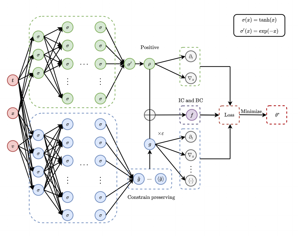
Same as in Section 3.1 the second equation yields g=1(𝒗𝒙ρ)𝑔superscript1𝒗subscript𝒙𝜌g=\mathcal{L}^{-1}(\bm{v}\cdot\nabla_{\bm{x}}\rho), which, when plugging into the first equation and integrating over v𝑣v, gived the diffusion equation (4). Hence this proposed method is an APNN method. Finally we put a schematic plot of our method in Figure 2.
Refer to caption
Figure 2: Schematic of APNNs for solving the linear transport equation with initial and boundary conditons.
Remark 2.

For the constraint g=0delimited-⟨⟩𝑔0\left\langle g\right\rangle=0, one way is to construct a novel neural network for g𝑔g such that it exactly satisfies g=0delimited-⟨⟩𝑔0\left\langle g\right\rangle=0. The other way is to treat it as a soft constraint with parameter λ3subscript𝜆3\lambda_{3}, i.e., without using (19), we use g^θNNsuperscriptsubscript^𝑔𝜃NN\hat{g}_{\theta}^{\text{NN}} and modifies the loss as

APNN, residual+λ3|𝒯×𝒟|𝒯𝒟|g~θNN0|2d𝒙dt.subscriptAPNN, residualsubscript𝜆3𝒯𝒟subscript𝒯subscript𝒟superscriptdelimited-⟨⟩subscriptsuperscript~𝑔NN𝜃02differential-d𝒙differential-d𝑡\mathcal{R}_{\text{APNN, residual}}+\frac{\lambda_{3}}{|\mathcal{T}\times\mathcal{D}|}\int_{\mathcal{T}}\int_{\mathcal{D}}|\left\langle\tilde{g}^{\text{NN}}_{\theta}\right\rangle-0|^{2}\mathop{}\!\mathrm{d}{\bm{x}}\mathop{}\!\mathrm{d}{t}. (42)

Our APNNs belongs to the first scenario. Specifically, in apnnsubscriptapnn\mathcal{R}_{\text{apnn}}, the integrand is not exactly the micro-macro decomposition in (23). Instead we replaced g𝑔g by gg𝑔delimited-⟨⟩𝑔g-\langle{g}\rangle since the later always satisfies =0delimited-⟨⟩0\langle{\cdot}\rangle=0, the desired conservation property! There are other terms in APNNεsubscriptsuperscript𝜀APNN\mathcal{R}^{\varepsilon}_{\text{APNN}} where such a change will not have any impact since the corresponding operators are invariant under such a transformation.

Remark 3.

The parity formulation (7) also allows one to construct AP schemes [36]. However if one uses it in the loss, it will not be an APNN. To see this, consider the case when ε0𝜀0\varepsilon\to 0. Since the DNN will only pick up the leading term, thus one has, in the L2superscript𝐿2L^{2} sense,

0=ρr,0𝜌𝑟\displaystyle 0=\rho-r, (43)
j=vσSxr.𝑗𝑣subscript𝜎𝑆subscript𝑥𝑟\displaystyle j=-\frac{v}{\sigma_{S}}\partial_{x}r\,.

These two equations will not lead to the diffusion equation (4).

5 Numerical examples

In this section, in order to verify and compare the performance of PINNs and APNNs, we present both 111D and 222D numerical results for several problems chosen from rarefied regimes (εO(1)𝜀𝑂1\varepsilon\approx O(1)) to hydrodynamic (diffusive) regimes (ε0𝜀0\varepsilon\to 0), including examples with high-dimensional uncertainties.

Since the losses of PINNs and APNNs are integrals, we approximate them by the Monte Carlo method by selecting small number of sub-domains randomly (batch size) and compute the operator delimited-⟨⟩\left\langle\cdot\right\rangle and Π()Π\Pi(\cdot) with quadrature rule. The optimization problem is solved by the Adam version of the gradient descent method [38]. The initial value of parameters set θ𝜃\theta in all numerical experiments are generated by Xavier initialization. All the hyper-parameters are chosen for best performance after trying these experiments. Specifically, in most of our experiments, we fix the x𝑥x domain as [0,1]01[0,1] and approximate the problem at randomly selected points {(ti,xi,vi)}subscript𝑡𝑖subscript𝑥𝑖subscript𝑣𝑖\{(t_{i},x_{i},v_{i})\}. It should be pointed out that the integral of v𝑣v for operator /delimited-⟨⟩\mathcal{L}/\left\langle\cdot\right\rangle is computed by quadrature rule (the Gauss-Legendre Integration). In detail, assume {wi,vi}i=1nsuperscriptsubscriptsubscript𝑤𝑖superscriptsubscript𝑣𝑖𝑖1𝑛\{{w_{i},v_{i}}^{\prime}\}_{i=1}^{n} are the nodes and weights, which {vi}i=1nsuperscriptsubscriptsuperscriptsubscript𝑣𝑖𝑖1𝑛\{{v_{i}}^{\prime}\}_{i=1}^{n} are the roots of the Legendre polynomials with degree n𝑛n and {wi}i=1nsuperscriptsubscriptsubscript𝑤𝑖𝑖1𝑛\{{w_{i}}\}_{i=1}^{n} are determined for accuracy. Then we can approximate an integral, for example, 11f(v)dvsuperscriptsubscript11𝑓𝑣differential-d𝑣\int_{-1}^{1}f(v)\mathop{}\!\mathrm{d}{v} by the summation of linear combination of f(vi):i=1nwif(vi):𝑓superscriptsubscript𝑣𝑖superscriptsubscript𝑖1𝑛subscript𝑤𝑖𝑓superscriptsubscript𝑣𝑖f({v_{i}}^{\prime}):\sum_{i=1}^{n}w_{i}f({v_{i}}^{\prime}).

The empirical risk for PINN is as follows

PINNε=subscriptsuperscript𝜀PINNabsent\displaystyle\mathcal{R}^{\varepsilon}_{\text{PINN}}= 1N1i=1N1|ε2tfθNN(ti,xi,vi)+ε𝒗xfθNN(ti,xi,vi)fθNN(ti,xi)ε2Q|21subscript𝑁1superscriptsubscript𝑖1subscript𝑁1superscriptsuperscript𝜀2subscript𝑡subscriptsuperscript𝑓NN𝜃subscript𝑡𝑖subscript𝑥𝑖subscript𝑣𝑖𝜀𝒗subscript𝑥subscriptsuperscript𝑓NN𝜃subscript𝑡𝑖subscript𝑥𝑖subscript𝑣𝑖subscriptsuperscript𝑓NN𝜃subscript𝑡𝑖subscript𝑥𝑖superscript𝜀2𝑄2\displaystyle\frac{1}{N_{1}}\sum_{i=1}^{N_{1}}\left|\varepsilon^{2}\partial_{t}f^{\text{NN}}_{\theta}(t_{i},x_{i},v_{i})+\varepsilon\bm{v}\cdot\nabla_{x}f^{\text{NN}}_{\theta}(t_{i},x_{i},v_{i})-\mathcal{L}f^{\text{NN}}_{\theta}(t_{i},x_{i})-\varepsilon^{2}Q\right|^{2} (44)
+λ1N2i=1N2|fθNN(ti,xi,vi)FB(ti,xi,vi)|2subscript𝜆1subscript𝑁2superscriptsubscript𝑖1subscript𝑁2superscriptsubscriptsuperscript𝑓NN𝜃subscript𝑡𝑖subscript𝑥𝑖subscript𝑣𝑖subscript𝐹Bsubscript𝑡𝑖subscript𝑥𝑖subscript𝑣𝑖2\displaystyle+\frac{\lambda_{1}}{N_{2}}\sum_{i=1}^{N_{2}}|\mathcal{B}f^{\text{NN}}_{\theta}(t_{i},x_{i},v_{i})-F_{\text{B}}(t_{i},x_{i},v_{i})|^{2}
+λ2N3i=1N3|fθNN(ti,xi,vi)f0(ti,xi,vi)|2,subscript𝜆2subscript𝑁3superscriptsubscript𝑖1subscript𝑁3superscriptsubscriptsuperscript𝑓NN𝜃subscript𝑡𝑖subscript𝑥𝑖subscript𝑣𝑖subscript𝑓0subscript𝑡𝑖subscript𝑥𝑖subscript𝑣𝑖2\displaystyle+\frac{\lambda_{2}}{N_{3}}\sum_{i=1}^{N_{3}}|\mathcal{I}f^{\text{NN}}_{\theta}(t_{i},x_{i},v_{i})-f_{0}(t_{i},x_{i},v_{i})|^{2},

where N1,N2,N3subscript𝑁1subscript𝑁2subscript𝑁3N_{1},N_{2},N_{3} are the number of sample points of 𝒯×𝒟×Ω,𝒯×𝒟×Ω,𝒟×Ω𝒯𝒟Ω𝒯𝒟Ω𝒟Ω\mathcal{T}\times\mathcal{D}\times\Omega,\mathcal{T}\times\partial\mathcal{D}\times\Omega,\mathcal{D}\times\Omega.

Similarly, the empirical risk for APNN is as follows

APNNε=subscriptsuperscript𝜀APNNabsent\displaystyle\mathcal{R}^{\varepsilon}_{\text{APNN}}= 1N1(1)i=1N1(1)|tρθNN(ti,xi)+x𝒗gθNN(ti,xi)Q|21superscriptsubscript𝑁11superscriptsubscript𝑖1superscriptsubscript𝑁11superscriptsubscript𝑡subscriptsuperscript𝜌NN𝜃subscript𝑡𝑖subscript𝑥𝑖subscript𝑥delimited-⟨⟩𝒗subscriptsuperscript𝑔NN𝜃subscript𝑡𝑖subscript𝑥𝑖𝑄2\displaystyle\frac{1}{N_{1}^{(1)}}\sum_{i=1}^{N_{1}^{(1)}}|\partial_{t}\rho^{\text{NN}}_{\theta}(t_{i},x_{i})+\nabla_{x}\cdot\left\langle\bm{v}g^{\text{NN}}_{\theta}\right\rangle(t_{i},x_{i})-Q|^{2} (45)
+1N1(2)i=1N1(2)|ε2tgθNN(ti,xi,vi)+ε(IΠ)(𝒗xgθNN)(ti,xi)conditional1superscriptsubscript𝑁12superscriptsubscript𝑖1superscriptsubscript𝑁12superscript𝜀2subscript𝑡subscriptsuperscript𝑔NN𝜃subscript𝑡𝑖subscript𝑥𝑖subscript𝑣𝑖𝜀𝐼Π𝒗subscript𝑥subscriptsuperscript𝑔NN𝜃subscript𝑡𝑖subscript𝑥𝑖\displaystyle+\frac{1}{N_{1}^{(2)}}\sum_{i=1}^{N_{1}^{(2)}}|\varepsilon^{2}\partial_{t}g^{\text{NN}}_{\theta}(t_{i},x_{i},v_{i})+\varepsilon(I-\Pi)(\bm{v}\cdot\nabla_{x}g^{\text{NN}}_{\theta})(t_{i},x_{i})
+𝒗i𝒙ρθNN(ti,xi)gθNN(ti,xi)(IΠ)εQ|2\displaystyle\quad+\bm{v}_{i}\cdot\nabla_{\bm{x}}\rho^{\text{NN}}_{\theta}(t_{i},x_{i})-{\mathcal{L}}g^{\text{NN}}_{\theta}(t_{i},x_{i})-(I-\Pi)\varepsilon Q|^{2}
+λ1N2i=1N2|(ρθNN(ti,xi)+εgθNN(ti,xi,vi))FB(ti,xi,vi)|2subscript𝜆1subscript𝑁2superscriptsubscript𝑖1subscript𝑁2superscriptsubscriptsuperscript𝜌NN𝜃subscript𝑡𝑖subscript𝑥𝑖𝜀subscriptsuperscript𝑔NN𝜃subscript𝑡𝑖subscript𝑥𝑖subscript𝑣𝑖subscript𝐹Bsubscript𝑡𝑖subscript𝑥𝑖subscript𝑣𝑖2\displaystyle+\frac{\lambda_{1}}{N_{2}}\sum_{i=1}^{N_{2}}|\mathcal{B}(\rho^{\text{NN}}_{\theta}(t_{i},x_{i})+\varepsilon g^{\text{NN}}_{\theta}(t_{i},x_{i},v_{i}))-F_{\text{B}}(t_{i},x_{i},v_{i})|^{2}
+λ2N3i=1N3|(ρθNN(ti,xi)+εgθNN(ti,xi,vi))f0(ti,xi,vi)|2.subscript𝜆2subscript𝑁3superscriptsubscript𝑖1subscript𝑁3superscriptsubscriptsuperscript𝜌NN𝜃subscript𝑡𝑖subscript𝑥𝑖𝜀subscriptsuperscript𝑔NN𝜃subscript𝑡𝑖subscript𝑥𝑖subscript𝑣𝑖subscript𝑓0subscript𝑡𝑖subscript𝑥𝑖subscript𝑣𝑖2\displaystyle+\frac{\lambda_{2}}{N_{3}}\sum_{i=1}^{N_{3}}|\mathcal{I}(\rho^{\text{NN}}_{\theta}(t_{i},x_{i})+\varepsilon g^{\text{NN}}_{\theta}(t_{i},x_{i},v_{i}))-f_{0}(t_{i},x_{i},v_{i})|^{2}.

where N1(1),N1(2),N2,N3superscriptsubscript𝑁11superscriptsubscript𝑁12subscript𝑁2subscript𝑁3N_{1}^{(1)},N_{1}^{(2)},N_{2},N_{3} are the number of sample points of 𝒯×𝒟,𝒯×𝒟×Ω,𝒯×𝒟×Ω,𝒟×Ω𝒯𝒟𝒯𝒟Ω𝒯𝒟Ω𝒟Ω\mathcal{T}\times\mathcal{D},\mathcal{T}\times\mathcal{D}\times\Omega,\mathcal{T}\times\partial\mathcal{D}\times\Omega,\mathcal{D}\times\Omega.

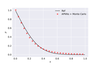
To investigate the influence of the Monte Carlo method in the integral with respect to v𝑣v, we conduct an extra experiment for the case ε=108𝜀superscript108\varepsilon=10^{-8} of Problem II. Besides, we show why the conservation is important for the same problem.

The reference solutions are obtained by standard finite difference methods. For most of the time we will check the relative 2superscript2\ell^{2} error of the density ρ(x)𝜌𝑥\rho(x) between DNN methods and reference solutions, e.g. for 111d case,

error:=j|ρθ,jNNρjref|2j|ρjref|2.assignerrorsubscript𝑗superscriptsubscriptsuperscript𝜌NN𝜃𝑗subscriptsuperscript𝜌ref𝑗2subscript𝑗superscriptsubscriptsuperscript𝜌ref𝑗2\text{error}:=\sqrt{\frac{\sum_{j}|\rho^{\text{NN}}_{\theta,j}-\rho^{\text{ref}}_{j}|^{2}}{\sum_{j}|\rho^{\text{ref}}_{j}|^{2}}}. (46)

5.1 One-dimensional problems

We shall consider different problems in slab geometry from the rarefied regimes (εO(1)𝜀𝑂1\varepsilon\approx O(1)) to the diffusive regimes (ε0𝜀0\varepsilon\to 0). Various boundary conditions and initial conditions will be used and both the transient and the steady state solutions will be presented with different ε𝜀\varepsilon’s.

Problem I. Smooth initial data with periodic BC

We start from the rarefied regimes where ε=1𝜀1\varepsilon=1 and consider periodic boundary condition with a smooth initial data as follows

f0(x,v)=ρ(x)2πev22,subscript𝑓0𝑥𝑣𝜌𝑥2𝜋superscript𝑒superscript𝑣22f_{0}(x,v)=\frac{\rho(x)}{\sqrt{2\pi}}e^{-\frac{v^{2}}{2}}, (47)

where

ρ(x)=1+cos(4πx).𝜌𝑥14𝜋𝑥\rho(x)=1+\cos(4\pi x). (48)

The source term, scattering and absorbing coefficients are set as

σS=1,σA=0,Q=0,ε=1.formulae-sequencesubscript𝜎𝑆1formulae-sequencesubscript𝜎𝐴0formulae-sequence𝑄0𝜀1\sigma_{S}=1,\quad\sigma_{A}=0,\quad Q=0,\quad\varepsilon=1. (49)

Enforcing exact periodic boundary is applied to improve the numerical performance. The ansatz is based on a Fourier basis and one can construct a transform T:x{sin(2πjx),cos(2πjx)}j=1k:𝑇𝑥superscriptsubscript2𝜋𝑗𝑥2𝜋𝑗𝑥𝑗1𝑘T:x\to\{\sin(2\pi jx),\cos(2\pi jx)\}_{j=1}^{k} before the first layer of DNN  [39, 40]. Here, we set k=2𝑘2k=2.

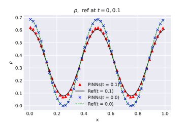
The result is shown in Figure 3 where we can find both PINN and APNN perform well.
Refer to caption
Refer to caption
Figure 3: Problems I. Plot of density ρ𝜌\rho at t=0.0,1.0𝑡0.01.0t=0.0,1.0. Left: PINNs vs. Ref, Right: APNNs vs. Ref. Neural networks are [5,128,128,128,128,1]51281281281281[5,128,128,128,128,1] for ρ𝜌\rho and [6,256,256,256,256,1]62562562562561[6,256,256,256,256,1] for g,f𝑔𝑓g,f. Batch size is 200020002000 in domain, 100010001000 with penalty λ2=1000subscript𝜆21000\lambda_{2}=1000 for initial condition, the number of quadrature points is 303030. Relative 2superscript2\ell^{2} error of PINNs and APNNs are 2.41×102,1.32×1022.41superscript1021.32superscript1022.41\times 10^{-2},1.32\times 10^{-2}.

Problem II. In-flow boundary condition

In the second example we consider the isotropic in-flow boundary conditions:

x[0,1],FL(v)=1,FR(v)=0.formulae-sequence𝑥01formulae-sequencesubscript𝐹𝐿𝑣1subscript𝐹𝑅𝑣0x\in[0,1],\quad F_{L}(v)=1,\quad F_{R}(v)=0. (50)

and initial condition f0(x,v)=0subscript𝑓0𝑥𝑣0f_{0}(x,v)=0. The source term, scattering and absorbing coefficients are set as

Q=0,σS=1,σA=0,ε=1,101,103,108.formulae-sequence𝑄0formulae-sequencesubscript𝜎𝑆1formulae-sequencesubscript𝜎𝐴0𝜀1superscript101superscript103superscript108Q=0,\quad\sigma_{S}=1,\quad\sigma_{A}=0,\quad\varepsilon=1,10^{-1},10^{-3},10^{-8}. (51)

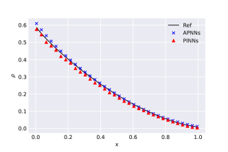
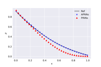
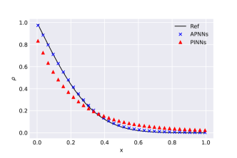
The results are shown in Figure 4 with exactly g=0delimited-⟨⟩𝑔0\left\langle g\right\rangle=0. Table 1 records the relative 2superscript2\ell^{2} errors of PINNs and APNNs in terms of penalty parameters (λ1,λ2)subscript𝜆1subscript𝜆2(\lambda_{1},\;\lambda_{2}) with ε=103𝜀superscript103\varepsilon=10^{-3}. One can find that the approximate accuracy is not good if λ1,λ2subscript𝜆1subscript𝜆2\lambda_{1},\lambda_{2} are too small or too large.

Refer to caption
(a) Density ρ𝜌\rho at t=1.0𝑡1.0t=1.0 with ε=1𝜀1\varepsilon=1.
Refer to caption
(b) Density ρ𝜌\rho at t=0.5𝑡0.5t=0.5 with ε=101𝜀superscript101\varepsilon=10^{-1}.
Refer to caption
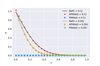
(c) Density ρ𝜌\rho at t=0.1𝑡0.1t=0.1 with ε=103𝜀superscript103\varepsilon=10^{-3}.
Refer to caption
(d) Density ρ𝜌\rho at t=0.05,0.1𝑡0.050.1t=0.05,0.1 with ε=108𝜀superscript108\varepsilon=10^{-8}.
Figure 4: Problems II. Plot of density ρ𝜌\rho for PINNs, APNNs and reference solutions. The number of quadrature points is 303030. Neural networks are (a𝑎a) to (b𝑏b): [2,128,128,128,128,1]21281281281281[2,128,128,128,128,1] for ρ𝜌\rho and [3,256,256,256,256,1]32562562562561[3,256,256,256,256,1] for g,f𝑔𝑓g,f. Batch size is 100010001000 for (a𝑎a) to (d𝑑d) in domain, (a𝑎a) and (b𝑏b): 400×24002400\times 2 with λ1=1subscript𝜆11\lambda_{1}=1; (c𝑐c) and (d𝑑d): 400×24002400\times 2 with λ1=10subscript𝜆110\lambda_{1}=10 for boundary condition, (a𝑎a) and (b𝑏b): 500500500 with λ2=1subscript𝜆21\lambda_{2}=1; (c𝑐c) and (d𝑑d): 100010001000 with λ2=10subscript𝜆210\lambda_{2}=10 for initial condition. Relative 2superscript2\ell^{2} errors of PINNs and APNNs are (a𝑎a): 4.01×102,1.36×1024.01superscript1021.36superscript1024.01\times 10^{-2},1.36\times 10^{-2}; (b𝑏b): 1.17×101,3.30×1021.17superscript1013.30superscript1021.17\times 10^{-1},3.30\times 10^{-2}; (c𝑐c): 2.17×101,1.98×1022.17superscript1011.98superscript1022.17\times 10^{-1},1.98\times 10^{-2}; (d𝑑d): 9.40×101,2.76×1029.40superscript1012.76superscript1029.40\times 10^{-1},2.76\times 10^{-2}, respectively.
(λ1,λ2)subscript𝜆1subscript𝜆2(\lambda_{1},\;\lambda_{2}) Error
PINNs APNNs
(1,   10) 7.09×1017.09superscript1017.09\times 10^{-1} 5.67×1025.67superscript1025.67\times 10^{-2}
(100,   10) 3.57×1013.57superscript1013.57\times 10^{-1} 4.72×1024.72superscript1024.72\times 10^{-2}
(10,   10) 2.17×1012.17superscript1012.17\times 10^{-1} 1.98×1021.98superscript1021.98\times 10^{-2}
(10,   1) 3.18×1013.18superscript1013.18\times 10^{-1} 1.11×1011.11superscript1011.11\times 10^{-1}
(10,   100) 5.52×1015.52superscript1015.52\times 10^{-1} 5.59×1025.59superscript1025.59\times 10^{-2}
Table 1: Problems II. Relative 2superscript2\ell^{2} errors of PINNs and APNNs in terms of penalty parameters (λ1,λ2)subscript𝜆1subscript𝜆2(\lambda_{1},\;\lambda_{2}) with ε=103𝜀superscript103\varepsilon=10^{-3}.

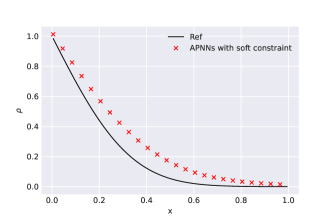
In the left of Figure 5, this conservation condition is not exactly satisfied by treating it as a soft constraint, i.e., using (42). Clearly failure to conserve the mass gives poor result. In Figure 4(d), for small ε𝜀\varepsilon PINN does not give accurate results while APNN gives quite accurate results for all ε𝜀\varepsilon tested. The right of Figure 5 shows the result where the integral with respect to v𝑣v is computed by the Monte Carlo method.
Refer to caption
Refer to caption
Figure 5: Problems II. Plot of density ρ𝜌\rho at t=0.1𝑡0.1t=0.1. Both neural networks are [2,128,256,256,128,1]21282562561281[2,128,256,256,128,1] for ρ𝜌\rho and [3,128,256,512,256,128,1]31282565122561281[3,128,256,512,256,128,1] for g𝑔g. Left : APNNs with soft constraint g=0delimited-⟨⟩𝑔0\left\langle g\right\rangle=0 vs. Ref. Batch size is 100010001000 in domain, 400×24002400\times 2 with penalty λ1=10subscript𝜆110\lambda_{1}=10 for boundary condition, 100010001000 with penalty λ2=10subscript𝜆210\lambda_{2}=10 for initial condition and penalty λ3=1subscript𝜆31\lambda_{3}=1 for constrain g=0delimited-⟨⟩𝑔0\left\langle g\right\rangle=0. Relative 2superscript2\ell^{2} error of APNNs with constrain g=0delimited-⟨⟩𝑔0\left\langle g\right\rangle=0 is 2.72×1012.72superscript1012.72\times 10^{-1}. Right: APNNs with integral by Monte Carlo method vs. Ref. Batch size is 800800800 in domain, 500×25002500\times 2 with penalty λ1=1subscript𝜆11\lambda_{1}=1 for boundary condition and 500500500 with penalty λ2=1subscript𝜆21\lambda_{2}=1 for initial condition, the number of quadrature points is 100100100. The number of sample is 100 for each iteration. The relative 2superscript2\ell^{2} error of APNNs with constraint g=0delimited-⟨⟩𝑔0\left\langle g\right\rangle=0 is 6.73×1026.73superscript1026.73\times 10^{-2}.

Problem III. A variable scattering coefficient

Let

x[0,1],FL(v)=1,FR(v)=0,formulae-sequence𝑥01formulae-sequencesubscript𝐹𝐿𝑣1subscript𝐹𝑅𝑣0x\in[0,1],\quad F_{L}(v)=1,\quad F_{R}(v)=0, (52)

and initial condition f0(x,v)=0subscript𝑓0𝑥𝑣0f_{0}(x,v)=0. The source term, scattering and absorbing coefficients are set as

Q=1,σS=1+(10x)2,σA=0,ε=0.01.formulae-sequence𝑄1formulae-sequencesubscript𝜎𝑆1superscript10𝑥2formulae-sequencesubscript𝜎𝐴0𝜀0.01Q=1,\quad\sigma_{S}=1+(10x)^{2},\quad\sigma_{A}=0,\quad\varepsilon=0.01. (53)

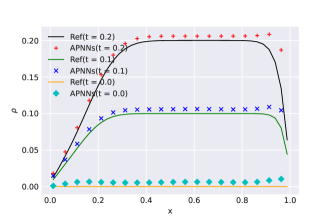
In Figure 6 we report the numerical solution by APNN at time t=0.0,0.1,0.2𝑡0.00.10.2t=0.0,0.1,0.2. In this problem we have a source term and the scattering cross section that depend on x𝑥x, so the scaling term σS/εsubscript𝜎𝑆𝜀\sigma_{S}/\varepsilon ranges from 1/εO(1)1𝜀𝑂11/\varepsilon\to O(1), a problem with mixing scales.The numerical results how reasonably good performance of APNN.
Refer to caption
Figure 6: Problems III. Plot of density ρ𝜌\rho with ε=102𝜀superscript102\varepsilon=10^{-2} at t=0.0,0.1,0.2𝑡0.00.10.2t=0.0,0.1,0.2 for APNNs and Reference solutions. Neural networks are [2,128,128,128,128,1]21281281281281[2,128,128,128,128,1] for ρ𝜌\rho and [3,256,256,256,256,1]32562562562561[3,256,256,256,256,1] for g𝑔g. Batch size is 500500500 in domain, 200×22002200\times 2 with penalty λ1=1subscript𝜆11\lambda_{1}=1 for boundary condition and 200200200 with penalty λ2=1subscript𝜆21\lambda_{2}=1 for initial condition, the number of quadrature points is 303030.

Problem IV. A problem with boundary layer

Let

x[0,1],FL(v)=5sin(v),FR(v)=0,formulae-sequence𝑥01formulae-sequencesubscript𝐹𝐿𝑣5𝑣subscript𝐹𝑅𝑣0x\in[0,1],\quad F_{L}(v)=5\sin(v),\quad F_{R}(v)=0, (54)

and initial condition f0(x,v)=0subscript𝑓0𝑥𝑣0f_{0}(x,v)=0. The source term, scattering and absorbing coefficients are set as

Q=0,σS=1,σA=0,ε=0.05.formulae-sequence𝑄0formulae-sequencesubscript𝜎𝑆1formulae-sequencesubscript𝜎𝐴0𝜀0.05Q=0,\quad\sigma_{S}=1,\quad\sigma_{A}=0,\quad\varepsilon=0.05. (55)

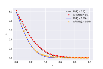
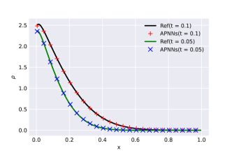
Here since FLsubscript𝐹𝐿F_{L} depends on v𝑣v, there is a boundary layer near x=0𝑥0x=0. Figure 7 shows that the boundary layer is well captured by APNN.
Refer to caption
Figure 7: Problems IV. Plot of density ρ𝜌\rho with ε=5×10²𝜀5superscript102\varepsilon=5\times 10^{-2} at t=0.05,0.1𝑡0.050.1t=0.05,0.1 for APNNs and Reference solutions.. Neural networks are [2,128,128,128,128,1]21281281281281[2,128,128,128,128,1] for ρ𝜌\rho and [3,256,256,256,256,1]32562562562561[3,256,256,256,256,1] for g𝑔g. Batch size is 100010001000 in domain, 400×24002400\times 2 with penalty λ1=10subscript𝜆110\lambda_{1}=10 for boundary condition and 100010001000 with penalty λ2=10subscript𝜆210\lambda_{2}=10 for initial condition, the number of quadrature points is 303030. Relative 2superscript2\ell^{2} error of APNNs is 4.80×1034.80superscript1034.80\times 10^{-3}.

5.2 Two-dimensional problems

Problem V. Rarefied regime

Consider a two dimensional problem with

Γ=[0,1]×[0,1],FB(𝒙,𝒗)=0,𝒏𝒗<0,𝒙Γ,formulae-sequenceΓ0101formulae-sequencesubscript𝐹𝐵𝒙𝒗0formulae-sequence𝒏𝒗0𝒙Γ\Gamma=[0,1]\times[0,1],\quad F_{B}(\bm{x},\bm{v})=0,\quad\bm{n}\cdot\bm{v}<0,\quad\bm{x}\in\partial\Gamma, (56)

and initial condition f0(x,v)=0subscript𝑓0𝑥𝑣0f_{0}(x,v)=0. The source term, scattering and absorbing coefficients are set as

Q=1,σS=1,σA=0,ε=1.formulae-sequence𝑄1formulae-sequencesubscript𝜎𝑆1formulae-sequencesubscript𝜎𝐴0𝜀1Q=1,\quad\sigma_{S}=1,\quad\sigma_{A}=0,\quad\varepsilon=1. (57)

Here 𝒏𝒏\bm{n} denotes the exterior unit normal vector on ΓΓ\partial\Gamma.

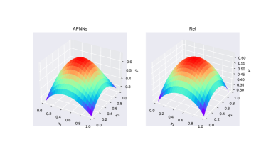
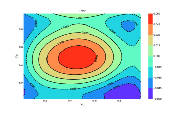
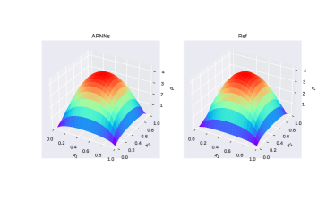
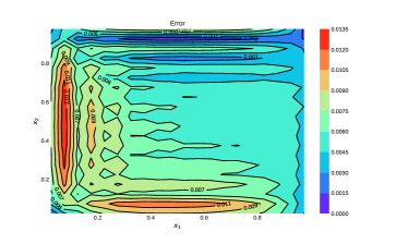
Figure 8 shows the density ρ𝜌\rho trained by APNNs and reference solution at time t=1.0𝑡1.0t=1.0 and the residual between them. The results show the good performance of APNNs with absolute error about 0.060.060.06 and relative 2superscript2\ell^{2} error 5.78×1025.78superscript1025.78\times 10^{-2}.

Refer to caption
Refer to caption
Figure 8: Problems V. Plot of density ρ𝜌\rho with ε=1𝜀1\varepsilon=1 at t=1.0𝑡1.0t=1.0 for APNNs and Reference solution. Neural networks are [3,64,128,256,1]3641282561[3,64,128,256,1] for ρ𝜌\rho and [5,64,128,256,512,1]5641282565121[5,64,128,256,512,1] for g𝑔g. Batch size is 800800800 in domain, 400×24002400\times 2 with penalty λ1=1subscript𝜆11\lambda_{1}=1 for boundary condition and 400400400 with penalty λ2=1subscript𝜆21\lambda_{2}=1 for initial condition, the number of quadrature points is 505050. Relative 2superscript2\ell^{2} error of APNNs is 5.78×1025.78superscript1025.78\times 10^{-2}.

Problem VI. A diffusive regime

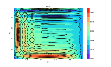
This test is a two dimensional test in the diffusive regime in which most of the setup are the same as previous example except ε=108𝜀superscript108\varepsilon=10^{-8} and Q=1,50𝑄150Q=1,50. Figure 9 show the density ρ𝜌\rho trained by APNNs and reference at time t=0.1𝑡0.1t=0.1 and corresponding residual error.

Refer to caption
Refer to caption
(a) Plot of density for APNNs and Reference solution. Left : Q=1𝑄1Q=1; Right : Q=50𝑄50Q=50.
Refer to caption
Refer to caption
(b) Residual. Left : Q=1𝑄1Q=1; Right : Q=50𝑄50Q=50.
Figure 9: Problems VI. Plot of density ρ𝜌\rho with ε=108𝜀superscript108\varepsilon=10^{-8} at t=0.1𝑡0.1t=0.1 for APNNs and Reference solution. Neural networks are [3,64,128,256,512,1]3641282565121[3,64,128,256,512,1] for ρ𝜌\rho and [5,64,128,256,512,1024,1]56412825651210241[5,64,128,256,512,1024,1] for g𝑔g. Batch size is 800800800 in domain, 400×24002400\times 2 with penalty λ1=1subscript𝜆11\lambda_{1}=1 for boundary condition and 400400400 with penalty λ2=1subscript𝜆21\lambda_{2}=1 for initial condition, the number of quadrature points is 505050. Relative 2superscript2\ell^{2} error of APNNs is 1.29×1021.29superscript1021.29\times 10^{-2} for Q=1𝑄1Q=1 and 4.35×1024.35superscript1024.35\times 10^{-2} for Q=50𝑄50Q=50.

5.3 Uncertainty quantification (UQ) problems

For the uncertainty quantification problem we consider the linear transport equation with a sine scattering function (ε=1,103𝜀1superscript103\varepsilon=1,{10}^{-3}) or Gaussian scattering function σS(𝒛)subscript𝜎𝑆𝒛\sigma_{S}(\bm{z}) (ε=108𝜀superscript108\varepsilon={10}^{-8}):

εtf+vxf=σS(𝒛)ε(1211f𝑑vf),xL<x<xR,1v1,formulae-sequenceformulae-sequence𝜀subscript𝑡𝑓𝑣subscript𝑥𝑓subscript𝜎𝑆𝒛𝜀12superscriptsubscript11𝑓differential-dsuperscript𝑣𝑓subscript𝑥𝐿𝑥subscript𝑥𝑅1𝑣1\varepsilon\partial_{t}f+v\partial_{x}f=\frac{\sigma_{S}(\bm{z})}{\varepsilon}\left(\frac{1}{2}\int_{-1}^{1}f\,dv^{\prime}-f\right),\quad x_{L}<x<x_{R},\quad-1\leq v\leq 1, (58)

with scattering coefficients

σS(𝒛)=1+0.3i=110sin(πzi),𝒛=(z1,z2,,z10)𝒰([1,1]10),formulae-sequencesubscript𝜎𝑆𝒛10.3superscriptsubscriptproduct𝑖110𝜋subscript𝑧𝑖𝒛subscript𝑧1subscript𝑧2subscript𝑧10similar-to𝒰superscript1110\sigma_{S}(\bm{z})=1+0.3\prod_{i=1}^{10}\sin(\pi z_{i}),\;\bm{z}=(z_{1},z_{2},\cdots,z_{10})\sim\mathcal{U}([-1,1]^{10}), (59)

or

σS(𝒛)=1+0.3exp(|𝒛|22),𝒛=(z1,z2,,z20)𝒰([3,3]20),formulae-sequencesubscript𝜎𝑆𝒛10.3superscript𝒛22𝒛subscript𝑧1subscript𝑧2subscript𝑧20similar-to𝒰superscript3320\sigma_{S}(\bm{z})=1+0.3\exp{\left(-\frac{|\bm{z}|^{2}}{2}\right)},\;\bm{z}=(z_{1},z_{2},\cdots,z_{20})\sim\mathcal{U}([-3,3]^{20}), (60)

initial condition f0(x,v)=0subscript𝑓0𝑥𝑣0f_{0}(x,v)=0, and in-flow boundary condition as,

f(t,xL=0,v)\displaystyle f(t,x_{L}=0,v) =FL(v)=1forv>0,formulae-sequenceabsentsubscript𝐹𝐿𝑣1for𝑣0\displaystyle=F_{L}(v)=1\quad\text{for}\quad v>0, (61)
f(t,xR=1,v)\displaystyle f(t,x_{R}=1,v) =FR(v)=0forv<0.formulae-sequenceabsentsubscript𝐹𝑅𝑣0for𝑣0\displaystyle=F_{R}(v)=0\quad\text{for}\quad v<0.

In this problem the 10-dimensional or 20-dimensional vector 𝒛𝒛\bm{z} represents the random input parameters in a typical uncertain problem setup [41]. Thus, m0=12,13subscript𝑚01213m_{0}=12,13 or 21,22212221,22 for ρ𝜌\rho and g𝑔g respectively. To compare numerical results, we evaluate ρ𝜌\rho at t=0.05,0.1𝑡0.050.1t=0.05,0.1 by taking expectation on 104superscript10410^{4} times simulations for (z1,,z10)subscript𝑧1subscript𝑧10(z_{1},\cdots,z_{10}) or (z1,,z20)subscript𝑧1subscript𝑧20(z_{1},\cdots,z_{20}). The goal of these examples is to show the ability of APNNs for high-dimensional problems.

Problem VII. UQ problem with ε=1𝜀1\varepsilon=1

Let ε=1𝜀1\varepsilon=1 and set scattering coefficients

σS(𝒛)=1+0.3i=110sin(πzi).subscript𝜎𝑆𝒛10.3superscriptsubscriptproduct𝑖110𝜋subscript𝑧𝑖\sigma_{S}(\bm{z})=1+0.3\prod_{i=1}^{10}\sin(\pi z_{i}). (62)

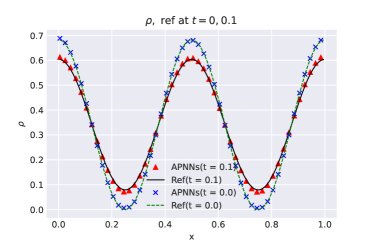
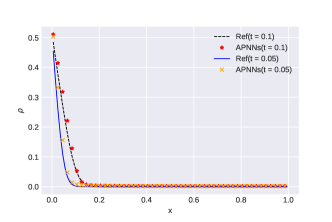
Figure 10 shows the density ρ𝜌\rho trained by APNNs and reference at time t=0.05,0.1𝑡0.050.1t=0.05,0.1. APNNs gives good approximation results.
Refer to caption
Figure 10: Problems VII. Plot of density ρ𝜌\rho by taking expectation for 𝒛𝒛\bm{z} at t=0.05,0.1𝑡0.050.1t=0.05,0.1 for APNNs and Reference solution. ε=1,σS(𝒛)=1+0.3i=110sin(πzi)formulae-sequence𝜀1subscript𝜎𝑆𝒛10.3superscriptsubscriptproduct𝑖110𝜋subscript𝑧𝑖\varepsilon=1,\sigma_{S}(\bm{z})=1+0.3\prod_{i=1}^{10}\sin(\pi z_{i}) and neural networks are [12,128,256,256,512,1]121282562565121[12,128,256,256,512,1] for ρ𝜌\rho and [13,128,256,512,1024,1]1312825651210241[13,128,256,512,1024,1] for g𝑔g. Batch size is 100010001000 in domain, 500×25002500\times 2 with penalty λ1=1subscript𝜆11\lambda_{1}=1 for boundary condition and 500500500 with penalty λ2=1subscript𝜆21\lambda_{2}=1 for initial condition, the number of quadrature points is 303030. Relative 2superscript2\ell^{2} error of APNNs is 8.78×1028.78superscript1028.78\times 10^{-2}.

Problem VIII. UQ problem with ε=103𝜀superscript103\varepsilon=10^{-3}

Let ε=103𝜀superscript103\varepsilon=10^{-3} and set scattering coefficients same as Problems VIII. Figure 11 shows the density ρ𝜌\rho trained by APNNs and reference at time t=0.05,0.1𝑡0.050.1t=0.05,0.1. APNN again gives quite good results.

Refer to caption
Figure 11: Problems VIII. Plot of density ρ𝜌\rho by taking expectation for 𝒛𝒛\bm{z} at t=0.05,0.1𝑡0.050.1t=0.05,0.1 for APNNs and Reference solution. ε=103,σS(𝒛)=1+0.3i=110sin(πzi)formulae-sequence𝜀superscript103subscript𝜎𝑆𝒛10.3superscriptsubscriptproduct𝑖110𝜋subscript𝑧𝑖\varepsilon=10^{-3},\sigma_{S}(\bm{z})=1+0.3\prod_{i=1}^{10}\sin(\pi z_{i}) and neural networks are [12,64,128,256,512,1]12641282565121[12,64,128,256,512,1] for ρ𝜌\rho and [13,64,128,256,512,1024,1]136412825651210241[13,64,128,256,512,1024,1] for g𝑔g. Batch size is 100010001000 in domain, 400×24002400\times 2 with penalty λ1=10subscript𝜆110\lambda_{1}=10 for boundary condition and 100010001000 with penalty λ2=10subscript𝜆210\lambda_{2}=10 for initial condition, the number of quadrature points is 303030. Relative 2superscript2\ell^{2} error of APNNs is 2.75×1022.75superscript1022.75\times 10^{-2}.

Problem IX. UQ problem with Gaussian scattering function

Consider the linear transport equation with ε=108𝜀superscript108\varepsilon=10^{-8} and scattering coefficients

σS(𝒛)=1+0.3exp(|𝒛|22),𝒛=(z1,z2,,z20)[3,3]20.formulae-sequencesubscript𝜎𝑆𝒛10.3superscript𝒛22𝒛subscript𝑧1subscript𝑧2subscript𝑧20superscript3320\sigma_{S}(\bm{z})=1+0.3\exp{\left(-\frac{|\bm{z}|^{2}}{2}\right)},\;\bm{z}=(z_{1},z_{2},\cdots,z_{20})\in[-3,3]^{20}. (63)

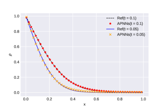
Figure 12 shows the density ρ𝜌\rho trained by APNNs and reference at time t=0.05,0.1𝑡0.050.1t=0.05,0.1. In this case one can also see good approximation results by APNN.
Refer to caption
Figure 12: Problems IX. Plot of density ρ𝜌\rho by taking expectation for 𝒛𝒛\bm{z} at t=0.05,0.1𝑡0.050.1t=0.05,0.1 for APNNs and Reference solution. ε=108,σS(𝒛)=1+0.3exp(|𝒛|2/2)formulae-sequence𝜀superscript108subscript𝜎𝑆𝒛10.3superscript𝒛22\varepsilon=10^{-8},\sigma_{S}(\bm{z})=1+0.3\exp{\left(-{|\bm{z}|^{2}}/{2}\right)} and neural networks are [22,64,128,256,512,1]22641282565121[22,64,128,256,512,1] for ρ𝜌\rho and [23,64,128,256,512,1024,1]236412825651210241[23,64,128,256,512,1024,1] for g𝑔g. Batch size is 100010001000 in domain, 400×24002400\times 2 with penalty λ1=10subscript𝜆110\lambda_{1}=10 for boundary condition and 100010001000 with penalty λ2=10subscript𝜆210\lambda_{2}=10 for initial condition, the number of quadrature points is 303030. Relative 2superscript2\ell^{2} error of APNNs is 1.51×1021.51superscript1021.51\times 10^{-2}.

6 Conclusion

In this paper we propose a deep neural network (DNN) for computing the multiscale uncertain linear transport equation with diffusive scaling. Our work follows the framework of Asymptotic-Preserving (AP) schemes for multiscale kinetic equations. We first point out that not all AP schemes will have the desired asymptotic structure when implementing them in the DNN framework. We design an AP neural network (APNN) by using the micro-macro decomposition, together with a mass conservation constraint in the loss function, that will have the desired AP properties, as will be shown by various multiscale and high-dimensional uncertain examples.

Acknowledgement

This work is partially supported by the National Key R&D Program of China Project No. 2020YFA0712000 and Shanghai Municipal of Science and Technology Major Project No. 2021SHZDZX0102. Shi Jin is also supported by NSFC grant No. 11871297. Zheng Ma is also supported by NSFC Grant No. 12031013 and partially supported by Institute of Modern Analysis – A Shanghai Frontier Research Center.

References

  • [1] Carlo Cercignani. The boltzmann equation. In The Boltzmann equation and its applications, pages 40–103. Springer, 1988.
  • [2] Shi Jin and Lorenzo Pareschi. Uncertainty quantification for hyperbolic and kinetic equations, volume 14. Springer, 2018.
  • [3] Jingwei Hu and Shi Jin. A stochastic galerkin method for the boltzmann equation with uncertainty. Journal of Computational Physics, 315:150–168, 2016.
  • [4] Shi Jin, Jian-Guo Liu, and Zheng Ma. Uniform spectral convergence of the stochastic Galerkin method for the linear transport equations with random inputs in diffusive regime and a micro–macro decomposition-based asymptotic-preserving method. Res. Math. Sci., 4:Paper No. 15, 25, 2017.
  • [5] Gaël Poëtte. A gpc-intrusive monte-carlo scheme for the resolution of the uncertain linear boltzmann equation. Journal of Computational Physics, 385:135–162, 2019.
  • [6] Gaël Poëtte. Numerical analysis of the monte-carlo noise for the resolution of the deterministic and uncertain linear boltzmann equation (comparison of non-intrusive gpc and mc-gpc). Journal of Computational and Theoretical Transport, pages 1–53, 2022.
  • [7] E Weinan. Principles of multiscale modeling. Cambridge University Press, 2011.
  • [8] François Bouchut, François Golse, and Mario Pulvirenti. Kinetic equations and asymptotic theory. Elsevier, 2000.
  • [9] Shi Jin. Asymptotic preserving (ap) schemes for multiscale kinetic and hyperbolic equations: a review. Lecture notes for summer school on methods and models of kinetic theory (M&MKT), Porto Ercole (Grosseto, Italy), pages 177–216, 2010.
  • [10] Pierre Degond and Fabrice Deluzet. Asymptotic-preserving methods and multiscale models for plasma physics. Journal of Computational Physics, 336:429–457, 2017.
  • [11] Jingwei Hu, Shi Jin, and Qin Li. Asymptotic-preserving schemes for multiscale hyperbolic and kinetic equations. In Handbook of Numerical Analysis, volume 18, pages 103–129. Elsevier, 2017.
  • [12] François Golse, Shi Jin, and C David Levermore. The convergence of numerical transfer schemes in diffusive regimes i: Discrete-ordinate method. SIAM journal on numerical analysis, 36(5):1333–1369, 1999.
  • [13] Lorenzo Pareschi and Russel E Caflisch. An implicit monte carlo method for rarefied gas dynamics: I. the space homogeneous case. Journal of Computational Physics, 154(1):90–116, 1999.
  • [14] Giacomo Dimarco and Lorenzo Pareschi. Numerical methods for kinetic equations. Acta Numerica, 23:369–520, 2014.
  • [15] Lorenzo Pareschi and Giovanni Russo. Time relaxed monte carlo methods for the boltzmann equation. SIAM Journal on Scientific Computing, 23(4):1253–1273, 2001.
  • [16] Weinan E and Bing Yu. The deep ritz method: A deep learning-based numerical algorithm for solving variational problems. Communications in Mathematics and Statistics, 6(1):1–12, 2018.
  • [17] Maziar Raissi, Paris Perdikaris, and George E Karniadakis. Physics-informed neural networks: A deep learning framework for solving forward and inverse problems involving nonlinear partial differential equations. Journal of Computational Physics, 378:686–707, 2019.
  • [18] Lu Lu, Pengzhan Jin, Guofei Pang, Zhongqiang Zhang, and George Em Karniadakis. Learning nonlinear operators via deeponet based on the universal approximation theorem of operators. Nature Machine Intelligence, 3(3):218–229, 2021.
  • [19] Zongyi Li, Nikola Kovachki, Kamyar Azizzadenesheli, Burigede Liu, Kaushik Bhattacharya, Andrew Stuart, and Anima Anandkumar. Fourier neural operator for parametric partial differential equations. arXiv preprint arXiv:2010.08895, 2020.
  • [20] Christian Beck, Martin Hutzenthaler, Arnulf Jentzen, and Benno Kuckuck. An overview on deep learning-based approximation methods for partial differential equations. arXiv preprint arXiv:2012.12348, 2020.
  • [21] Yulei Liao and Pingbing Ming. Deep Nitsche method: Deep Ritz method with essential boundary conditions. arXiv preprint arXiv:1912.01309, 2019.
  • [22] Justin Sirignano and Konstantinos Spiliopoulos. DGM: A deep learning algorithm for solving partial differential equations. Journal of Computational Physics, 375:1339–1364, 2018.
  • [23] Yaohua Zang, Gang Bao, Xiaojing Ye, and Haomin Zhou. Weak adversarial networks for high-dimensional partial differential equations. Journal of Computational Physics, page 109409, 2020.
  • [24] Zhiqiang Cai, Jingshuang Chen, and Min Liu. Least-squares relu neural network (lsnn) method for linear advection-reaction equation. Journal of Computational Physics, page 110514, 2021.
  • [25] Liyao Lyu, Zhen Zhang, Minxin Chen, and Jingrun Chen. MIM: A deep mixed residual method for solving high-order partial differential equations. arXiv preprint arXiv:2006.04146, 2020.
  • [26] Hyung Ju Hwang, Jin Woo Jang, Hyeontae Jo, and Jae Yong Lee. Trend to equilibrium for the kinetic fokker-planck equation via the neural network approach. Journal of Computational Physics, 419:109665, 2020.
  • [27] Zheng Chen, Liu Liu, and Lin Mu. Solving the linear transport equation by a deep neural network approach. arXiv preprint arXiv:2102.09157, 2021.
  • [28] Long Li and Chang Yang. Asymptotic preserving scheme for anisotropic elliptic equations with deep neural network. arXiv preprint arXiv:2104.05337, 2021.
  • [29] Ricardo A Delgadillo, Jingwei Hu, and Haizhao Yang. Multiscale and nonlocal learning for pdes using densely connected rnns. arXiv preprint arXiv:2109.01790, 2021.
  • [30] Qin Lou, Xuhui Meng, and George Em Karniadakis. Physics-informed neural networks for solving forward and inverse flow problems via the boltzmann-bgk formulation. Journal of Computational Physics, 447:110676, 2021.
  • [31] Lu Lu, Xuhui Meng, Zhiping Mao, and George Em Karniadakis. Deepxde: A deep learning library for solving differential equations. SIAM Review, 63(1):208–228, 2021.
  • [32] Zhi-Qin John Xu, Yaoyu Zhang, Tao Luo, Yanyang Xiao, and Zheng Ma. Frequency principle: Fourier analysis sheds light on deep neural networks. arXiv preprint arXiv:1901.06523, 2019.
  • [33] Subrahmanyan Chandrasekhar. Radiative transfer. Courier Corporation, 2013.
  • [34] Leonid Ryzhik, George Papanicolaou, and Joseph B Keller. Transport equations for elastic and other waves in random media. Wave motion, 24(4):327–370, 1996.
  • [35] Claude Bardos, Rafael Santos, and Rémi Sentis. Diffusion approximation and computation of the critical size. Transactions of the american mathematical society, 284(2):617–649, 1984.
  • [36] Shi Jin, Lorenzo Pareschi, and Giuseppe Toscani. Uniformly accurate diffusive relaxation schemes for multiscale transport equations. SIAM Journal on Numerical Analysis, 38(3):913–936, 2000.
  • [37] Mohammed Lemou and Luc Mieussens. A new asymptotic preserving scheme based on micro-macro formulation for linear kinetic equations in the diffusion limit. SIAM Journal on Scientific Computing, 31(1):334–368, 2008.
  • [38] Diederik P Kingma and Jimmy Ba. Adam: A method for stochastic optimization. In ICLR, 2015.
  • [39] Jiequn Han, Jianfeng Lu, and Mo Zhou. Solving high-dimensional eigenvalue problems using deep neural networks: A diffusion monte carlo like approach. Journal of Computational Physics, 423:109792, 2020.
  • [40] Liyao Lyu, Keke Wu, Rui Du, and Jingrun Chen. Enforcing exact boundary and initial conditions in the deep mixed residual method. CSIAM Transactions on Applied Mathematics, 2(4):748–775, 2021.
  • [41] Shi Jin, Dongbin Xiu, and Xueyu Zhu. Asymptotic-preserving methods for hyperbolic and transport equations with random inputs and diffusive scalings. Journal of Computational Physics, 289:35–52, 2015.