Higher-order non-global logarithms from jet calculus

Abstract

Non-global QCD observables are characterised by a sensitivity to the full angular distribution of soft radiation emitted coherently in hard scattering processes. This complexity poses a challenge to their all-order resummation, that was formulated at the leading-logarithmic order about two decades ago. In this article we present a solution to the long-standing problem of their resummation beyond this order, and carry out the first complete next-to-leading logarithmic calculation for non-global observables. This is achieved by solving numerically the recently derived set of non-linear differential equations which describe the evolution of soft radiation in the planar, large-$N_{c}$ limit. As a case study we address the calculation of the transverse energy distribution in the interjet rapidity region in $e^{+}e^{-}\to$ dijet production. The calculation is performed by means of an algorithm that we formulate in the language of jet-calculus generating functionals, which also makes the resummation technique applicable to more general non-global problems, such as those that arise in hadronic collisions. We find that NLL corrections are substantial and their inclusion leads to a significant reduction of the perturbative scale uncertainties for these observables. The computer code used in the calculations is made publicly available.

1 Introduction

The topic of non-global QCD observables Dasgupta:2001sh has received significant attention in recent years. A first reason is due to their theoretical complexity. These observables are characterised by kinematic constraints on limited angular regions of the radiation phase space, which leads to a rich structure in perturbation theory. This class of logarithmic corrections to physical observables was discovered and resummed at leading logarithmic (LL) order in the planar, large-number-of-colour (large-$N_{c}$) limit about 20 years ago Dasgupta:2001sh ; Dasgupta:2002bw ; Banfi:2002hw , and methods to calculate finite-$N_{c}$ effects are also well established Hatta:2013iba ; Hagiwara:2015bia ; Hatta:2020wre . While subleading-colour corrections are commonly numerically small in known applications, their study is of importance for the understanding of the structure of super-leading logarithmic corrections in non-global observables at hadron colliders Forshaw:2006fk ; Forshaw:2008cq ; Becher:2021zkk .

The calculation of non-global corrections to higher orders largely remains an open problem. Several new formulations of the resummation have been proposed in recent years Becher:2015hka ; Becher:2016mmh ; Caron-Huot:2015bja ; Larkoski:2015zka ; Banfi:2021owj , accompanying a large amount of applications to perturbative calculations of collider observables at LL, and recently also including some class of NLL corrections (see e.g. Forshaw:2009fz ; Rubin:2010fc ; Banfi:2010pa ; DuranDelgado:2011tp ; Dasgupta:2012hg ; Schwartz:2014wha ; Becher:2015hka ; Becher:2016omr ; Neill:2016stq ; Caron-Huot:2016tzz ; Larkoski:2016zzc ; Becher:2017nof ; Martinez:2018ffw ; Balsiger:2018ezi ; Neill:2018yet ; Neill:2018yet ; Balsiger:2019tne ; Balsiger:2020ogy ; Ziani:2021dxr ). Their study is also motivated by theoretical interests related to the connection between their dynamics and the high-energy limit of scattering amplitudes Weigert:2003mm ; Hatta:2008st ; Caron-Huot:2015bja .

A second reason why non-global observables are interesting is their ubiquitous occurence at colliders, for instance via the use of jets or often when specific fiducial cuts are applied in experimental measurements. In the context of the precision physics programme of present and future particle colliders, it is therefore paramount to gain theoretical control over non-global corrections to physical observables.

Finally, an understanding of their dynamics is instrumental in the context of developing more accurate parton-shower algorithms (see e.g. Refs. Dasgupta:2018nvj ; Bewick:2019rbu ; Dasgupta:2020fwr ; Forshaw:2020wrq ; Platzer:2020lbr ; Hamilton:2020rcu ; Nagy:2020rmk ; Nagy:2020dvz ; Karlberg:2021kwr ; Dulat:2018vuy ; Gellersen:2021eci ; Hamilton:2021dyz ). Specifically, the resummation of next-to-leading logarithmic (NLL) non-global logarithms is a crucial ingredient for the development of NNLL algorithms, that are necessary to achieve sufficiently accurate event simulation both at present and future colliders.

In a recent article Banfi:2021owj we have developed a framework for the resummation of non-global observables in the planar limit, which relies on a set of non-linear evolution equations that describe the dynamics of soft radiation at different energy scales. Ref. Banfi:2021owj also demonstrates the correctness of the framework by comparing a calculation at fixed perturbative order in this formalism to the full QCD result for the energy and transverse energy distributions in the rapidity gap between two cone jets produced in electron-positron annihilation.

In this article, we instead address the solution of the equations of Ref. Banfi:2021owj at all perturbative orders, hereby achieving a first complete NLL resummation for a non-global observable in the large-$N_{c}$ limit. The paper is structured as follows. Sec. 2 contains a summary of the findings of Ref. Banfi:2021owj . Sec. 3 reformulates the evolution equations in terms of a well known method used in jet calculus, that of generating functionals Konishi:1979cb ; Bassetto:1984ik ; Dokshitzer:1991wu . This formulation has two important advantages. Firstly, it provides us with a probabilistic picture to solve the evolution equations using a Markov chain Monte-Carlo algorithm. Secondly, the resulting algorithm describing the evolution of the soft radiation in the planar limit is independent of the underlying hard scattering process, and therefore can be readily applied to other observables and reactions, such as jet production at hadron colliders. The algorithm is given in detail in Sec. 4, which is arguably the most technical part of the article. The reader uninterested in the technical aspects of the calculation can skip directly from Sec. 3 to Sec. 5 where the numerical results are presented. In Sec. 5 we report NLL predictions for the transverse energy distribution in the interjet rapidity slice in $e^{+}e^{-}\to\,2$ jets, and discuss the impact of NLL corrections as well as the reduction in the perturbative uncertainty. Finally, Sec. 6 contains our conclusions.

2 Resummation for $E_{t}$ in the interjet rapidity gap

As in ref. Banfi:2021owj , we consider the production of two jets in $e^{+}e^{-}$ annihilation at a centre-of-mass energy $\sqrt{s}$. We study a non-global observable defined by measuring hadrons in a rapidity slice between the two jets. This is defined as the rapidity region between two cones of opening angle $\theta_{\rm jet}$ around the thrust axis (see Fig. 1). The width of such a rapidity slice is

$$\Delta\eta\coloneqq\ln\frac{1+c}{1-c}\,,\qquad c=\cos\theta_{\rm jet}\,.$$ (1)

Figure 1: The rapidity slice where the measurement is performed.

Examples of non-global observables are those studied in ref. Banfi:2021owj , namely the total energy or transverse energy of hadrons inside the slice. In the following we consider the latter for the sake of arguments, although the formalism introduced in this section also applies to the calculation of the energy distribution.

The cumulative distribution for this observable to be less than $v\equiv E_{t}$ is defined as follows

$$\Sigma(v)\coloneqq\frac{1}{\sigma_{0}}\int_{0}^{v}\frac{d\sigma}{dv^{\prime}}dv^{\prime}\,,$$ (2)

where $\sigma_{0}$ is the Born cross section for $e^{+}e^{-}\to$ hadrons. Without any emissions, at the lowest order in perturbation theory, $\Sigma(v)=1$, and the event is made up of a quark of momentum $p_{1}$ and an antiquark of momentum $p_{2}$, back-to-back and aligned along the thrust axis. When extra radiation is considered, $\Sigma(v)$ can be expressed as Banfi:2021owj

$$\Sigma(v)\coloneqq\sum_{n=2}^{\infty}{\cal H}_{n}\otimes S_{n}(v)={\cal H}_{2}\otimes S_{2}(v)+{\cal H}_{3}\otimes S_{3}(v)+\cdots$$ (3)

where the hard factors

$${\cal H}_{n}\coloneqq{\cal H}_{1\dots n}$$ (4)

describe configurations with $n$ hard QCD partons along the light-like directions $n_{1},\dots,n_{n}$ (with $n^{2}_{i}=0$ and $|\vec{n}|^{2}=1$), while the soft factors

$$S_{n}\coloneqq S_{1\dots n}$$ (5)

describe the emission of soft radiation off a hard system with $n$ hard emitters along the same directions. The convolutions in Eq. (3) are meant to indicate that the directions of the hard emitters in the hard and soft factors are the same, namely

$${\cal H}_{n}\otimes S_{n}(v)\coloneqq\int\left(\prod_{i=i}^{n}d^{2}\Omega_{i}\right){\cal H}_{1\dots n}\times S_{1\dots n}(v),$$ (6)

where $\Omega_{i}$ indicates the solid angle of the $i$-th hard emitter, namely the direction of the $\vec{n}_{i}$ vector, specified by a longitudinal ($\theta$) and an azimuthal ($\phi$) angle. In writing Eq. (6) we assumed that all IRC divergences cancel in the definition of ${\cal H}_{n}$ and $S_{n}$, and the four-dimensional limit can be taken in the angular integration Banfi:2021owj . Each of the above ingredients admits a perturbative expansion in the strong coupling constant Banfi:2021owj

$${\cal H}_{n}=\sum_{i=n-2}^{\infty}\frac{\alpha_{s}^{i}}{(2\pi)^{i}}{\cal H}_{n}^{(i)},\qquad S_{n}=\sum_{i=0}^{\infty}\frac{\alpha_{s}^{i}}{(2\pi)^{i}}S_{n}^{(i)},$$ (7)

where the normalisation is defined such that at the Born level one has

$${\cal H}_{2}^{(0)}=\delta^{(2)}(\Omega_{1}-\Omega_{q})\delta^{(2)}(\Omega_{2}-\Omega_{\bar{q}})\coloneqq\delta(\cos\theta_{1}-1)\delta(\cos\theta_{2}+1)\delta(\phi_{1})\delta(\phi_{2})\,,\quad S_{n}^{(0)}=1\,.$$ (8)

At LL, the cumulative distribution is given by the convolution of the LO hard factor ${\cal H}_{2}$ with the LL soft factor $S_{2}$. At NLL, one needs to include the LO hard factor ${\cal H}_{3}$ convoluted with the LL soft factor $S_{3}$, as well as the NLO hard factor ${\cal H}_{2}$ convoluted with the NLL soft factor $S_{2}$.

The observables considered in ref. Banfi:2021owj were all additive, which implies that the observable constraint on the soft emissions contributing to $S_{n}$ factorises under the Laplace transform

$$\Theta\left(v-\sum_{i}v(k_{i})\Theta_{\rm in}(k_{i})\right)=\frac{1}{2\pi i}\int_{\gamma}\frac{d\nu}{\nu}e^{\nu v}\prod_{i}u(k_{i})\,,$$ (9)

where the trigger function $\Theta_{\rm in}(k)$ is 1 if the particle $k$ is inside the measurement region, and zero otherwise, and the contour $\gamma$ lies parallel to the imaginary axis and to the right of all singularities of the integrand. The quantity $u(k)$ is the following “source” function:

$$u(k)=\Theta_{\rm out}(k)+\Theta_{\rm in}(k)e^{-\nu v(k)}\,,$$ (10)

with $\Theta_{\rm out}(k)=1-\Theta_{\rm in}(k)$. Following ref. Banfi:2021owj , in the large-$N_{c}$ limit we can then define the Laplace transform of the soft factors entering the NLL calculation

$$\begin{split}S_{2}(v)=\frac{1}{2\pi i}\int_{\gamma}\frac{d\nu}{\nu}e^{\nu v}G_{12}[Q;u]\,,\quad S_{3}(v)=\frac{1}{2\pi i}\int_{\gamma}\frac{d\nu}{\nu}e^{\nu v}G_{13}[Q;u]G_{23}[Q;u]\,.\end{split}$$ (11)

The evolution of the $G_{ij}[Q;u]$ functionals is governed by the differential equation (in the following we set $\{ij\}=\{12\}$ unless otherwise specified, but the same considerations hold for the evolution of a generic dipole $\{ij\}$)

$$Q\partial_{Q}G_{12}[Q;u]={\mathbb{K}}[G[Q;u],u]\,.$$ (12)

The evolution kernels are derived in Ref. Banfi:2021owj , and we report them in $4-2\epsilon$ dimensions below. The LL kernel, relevant for the evolution of $S_{3}$ reads

$${\mathbb{K}}^{\rm LL} [G[Q;u],u]\coloneqq\int[dk_{a}]\bar{\alpha}(Q)w^{(0)}_{12}(k_{a})$$ (13)

$$\hskip 28.45274pt\times\left(G_{1a}[Q;u]G_{a2}[Q;u]u(k_{a})-G_{12}[Q;u]\right)Q\delta(Q-k_{ta})\,.$$

The tree-level eikonal squared amplitude is defined as

$$w^{(0)}_{ij}(k)=8\pi^{2}\frac{\mu^{2\epsilon}}{k_{t}^{2}}\,,\quad k_{t}^{2}\coloneqq(k_{t}^{(ij)})^{2}=2\frac{(k_{i}\cdot k)(k\cdot k_{j})}{(k_{i}\cdot k_{j})}\,,$$ (14)

where $k_{t}$ denotes the transverse momentum of emission $k$ w.r.t. the emitting $\{ij\}$ dipole (note that in the equation above $k_{i,j}\equiv p_{i,j}$ if it refers to one of the hard legs). In the same variables, the corresponding phase space measure in $4-2\epsilon$ dimensions reads

$$[dk]\coloneqq\frac{d\eta}{2}\frac{d^{2-2\epsilon}k_{t}}{(2\pi)^{3-2\epsilon}}\,,$$ (15)

where the rapidity bound in the soft limit is given by

$$|\eta|\lesssim\ln\frac{\sqrt{2\,k_{i}\cdot k_{j}}}{k_{t}}\,.$$ (16)

A discussion about the choice of ordering variable and its relation to symmetries of the multi-particle squared amplitude is reported in Appendix A. In Eq. (13) we also defined $\bar{\alpha}=N_{c}\alpha_{s}(\mu)/\pi$, where $\alpha_{s}$ is the QCD coupling in the $\overline{\rm MS}$ scheme, satisfying the renormalisation group equation (RGE)

$$\frac{d\bar{\alpha}(\mu)}{d\ln\mu^{2}}=-\bar{\beta}(\bar{\alpha})=-\bar{\alpha}\left(\bar{\beta}_{0}\bar{\alpha}+\bar{\beta}_{1}\bar{\alpha}^{2}+\dots\right)\,,$$ (17)

where $\bar{\beta}_{i}$ are obtained from the large-$N_{c}$ limit of the coefficients of the QCD beta function as

$$\bar{\beta}_{i}=\lim_{N_{c}\to\infty}\left(\frac{\pi}{N_{c}}\right)^{i+1}\beta_{i}\,.$$ (18)

We work in the normalisation in which $\beta_{0}=(11C_{A}-2n_{F})/(12\pi)$ and $\bar{\beta}_{0}=11/12$. The coupling in the LL kernel (13) evolves at one loop (i.e. setting $\bar{\beta}_{1}=0$ in Eq. (17)), while it evolves at two loops in the NLL kernel defined in the following. The NLL kernel which governs the evolution of $S_{2}$ reads

$${\mathbb{K}}^{\rm NLL}[G[Q;u],u]\coloneqq{\mathbb{K}}^{\rm RV+VV}[G[Q;u],u]+{\mathbb{K}}^{\rm RR}[G[Q;u],u]-{\mathbb{K}}^{\rm DC}[G[Q;u],u]\,.$$ (19)

The three contributions to the above equation describe three sources of NLL corrections. The kernel correction due to the subtracted virtual and real-virtual corrections reads

$${\mathbb{K}}^{\rm RV+VV} [G[Q;u],u]\coloneqq\int[dk_{a}]\bar{\alpha}(Q)w^{(0)}_{12}(k_{a})\,\bigg{(}1+\bar{\alpha}(Q)\,\bar{K}^{(1)}\bigg{)}$$ (20)

$$\hskip 28.45274pt\times\left(G_{1a}[Q;u]G_{a2}[Q;u]u(k_{a})-G_{12}[Q;u]\right)Q\delta(Q-k_{ta})\,,$$

where $\bar{K}^{(1)}$ is obtained from the two-loop cusp anomalous dimension in the large-$N_{c}$ limit

$$\bar{K}^{(1)}=\lim_{N_{c}\to\infty}\frac{2}{N_{c}}\,K^{(1)}=\frac{67}{36}-\frac{\pi^{2}}{12}\,.$$ (21)

Then, the double real corrections are given by

$${\mathbb{K}}^{\rm RR} [G[Q;u],u]\coloneqq\int[dk_{a}]\int[dk_{b}]\,\bar{\alpha}^{2}(Q)Q\delta(Q-k_{t(ab)}){\Theta(k_{ta}-k_{tb}^{\prime})}$$ (22)

$$\times\left[\bar{w}^{(gg)}_{12}(k_{b},k_{a})G_{1b}[Q;u]G_{ba}[Q;u]G_{a2}[Q;u]u(k_{a})u(k_{b})\right.$$

$$\left.\hskip 28.45274pt+\bar{w}^{(gg)}_{12}(k_{a},k_{b})G_{1a}[Q;u]G_{ab}[Q;u]G_{b2}[Q;u]u(k_{a})u(k_{b})\right.$$

$$\left.\hskip 56.9055pt-\left(\bar{w}^{(gg)}_{12}(k_{b},k_{a})+\bar{w}^{(gg)}_{12}(k_{a},k_{b})\right)G_{1(ab)}[Q;u]G_{(ab)2}[Q;u]u(k_{(ab)})\right]\,,$$

where $k_{tb}^{\prime}$ denotes the transverse momentum of $k_{b}$ with respect of the $\{12\}$ dipole, namely

$$(k_{tb}^{\prime})^{2}=2\frac{(p_{1}\cdot k_{b})(k_{b}\cdot p_{2})}{(p_{1}\cdot p_{2})}\,.$$ (23)

To properly define $\bar{w}^{(gg)}_{12}(k_{a},k_{b})$ we need first to introduce the colour-ordered double soft squared amplitude at tree level Campbell:1997hg ; GehrmannDeRidder:2005cm

$$\tilde{w}^{(0)}_{12}(k_{a},k_{b}) =2\,(2\pi)^{4}\mu^{4\epsilon}\bigg{[}\frac{s_{12}^{2}}{s_{1a}s_{ab2}s_{1ab}s_{b2}}+\frac{1-\epsilon}{s_{ab}^{2}}\left(\frac{s_{1a}}{s_{1ab}}+\frac{s_{b2}}{s_{ab2}}-1\right)^{2}$$

$$+\frac{s_{12}}{s_{ab}}\left(\frac{1}{s_{1a}s_{b2}}+\frac{1}{s_{1a}s_{ab2}}+\frac{1}{s_{b2}s_{1ab}}-\frac{4}{s_{1ab}s_{ab2}}\right)\bigg{]}\,,$$ (24)

where the Lorentz invariants $s_{i\dots k}$ indicate the standard Mandelstam variables. Following Banfi:2021owj , we define $\bar{w}^{(gg)}_{12}(k_{a},k_{b})$ as the correlated contribution to $\tilde{w}^{(0)}_{12}(k_{a},k_{b})$, as follows

$$\bar{w}^{(gg)}_{12}(k_{a},k_{b})\coloneqq\tilde{w}^{(0)}_{12}(k_{a},k_{b})-\frac{1}{2}w^{(0)}_{12}(k_{a})w^{(0)}_{12}(k_{b})\,,$$ (25)

where $\frac{1}{2}w^{(0)}_{12}(k_{a})w^{(0)}_{12}(k_{b})$ represents the independent emission contribution. The counter-term in the r.h.s. of Eq. (22) is built upon the massless momentum $k_{(ab)}$ defined by the following kinematic map

$${\mathbb{P}}:\{k_{a},k_{b}\}\rightarrow k_{(ab)}={\left(k_{t(ab)}\cosh\eta_{(ab)},\vec{k}_{t(ab)},k_{t(ab)}\sinh\eta_{(ab)}\right)}\,,$$ (26)

where $k_{t(ab)}$ and $\eta_{(ab)}$ denote the transverse momentum and rapidity of $k_{a}+k_{b}$ in the $\{12\}$ dipole rest frame. Eq. (26) is expressed in the $\{12\}$ dipole rest frame where the $\{12\}$ dipole is aligned with the $z$ axis. A Lorentz transformation (a rotation followed by a boost) must be then applied to $k_{(ab)}$ to express it in the event frame. Last, we subtract the iteration of the LL kernel

$${\mathbb{K}}^{\rm DC} [G[Q;u],u]\coloneqq\int[dk_{a}]\int[dk_{b}]\bar{\alpha}^{2}(Q)Q\delta(Q-k_{ta})\Theta(k_{ta}-k_{tb})$$ (27)

$$\times\biggl{[}w^{(0)}_{12}(k_{a})\left(w^{(0)}_{1a}(k_{b})-\frac{1}{2}w^{(0)}_{12}(k_{b})\right)G_{1b}[Q;u]G_{ba}[Q;u]G_{a2}[Q;u]u(k_{a})u(k_{b})$$

$$\hskip 28.45274pt+w^{(0)}_{12}(k_{a})\left(w^{(0)}_{a2}(k_{b})-\frac{1}{2}w^{(0)}_{12}(k_{b})\right)G_{1a}[Q;u]G_{ab}[Q;u]G_{b2}[Q;u]u(k_{a})u(k_{b})$$

$$\hskip 56.9055pt-w^{(0)}_{12}(k_{a})\left(w^{(0)}_{1a}(k_{b})+w^{(0)}_{a2}(k_{b})-w^{(0)}_{12}(k_{b})\right)G_{1a}[Q;u]G_{a2}[Q;u]u(k_{a})\biggr{]}\,.$$

In the above expression, with a little abuse of notation, we denoted with $k_{tb}$ the transverse momentum of $k_{b}$ with respect to the emitting dipole, that is each term should be interpreted as follows

$$w^{(0)}_{ij}(k_{b})\Theta(k_{ta}-k_{tb})\coloneqq w^{(0)}_{ij}(k_{b})\Theta(k_{ta}-k^{(ij)}_{tb})\,,$$ (28)

where $k^{(ij)}_{tb}$ is the transverse momentum of $k_{b}$ with respect to the “emitting” dipole $\{ij\}$ (see also Eq. (14))

$$(k^{(ij)}_{tb})^{2}=2\frac{(k_{i}\cdot k_{b})(k_{b}\cdot k_{j})}{(k_{i}\cdot k_{j})}\,,$$ (29)

with $k_{i,j}\equiv p_{i,j}$ if it refers to one of the hard legs. The quantity $G_{ij}$ satisfies the boundary condition

$$G_{ij}[Q;u]=1~{}{\rm for}~{}Q=0\,,$$ (30)

and the normalisation $G_{ij}[Q;1]=1$. In taking the four-dimensional limit of the above equations some care is required since the boundary condition has to be deformed by introducing an appropriate non-perturbative prescription. In this article we consider implementing the following procedure Banfi:2021owj

$$\alpha_{s}(k)=\alpha_{s}(Q_{0})=0,\qquad k\leq Q_{0}\,,$$ (31)

where $Q_{0}$ is defined below (see Eq. (51)) and it is above the Landau singularity. This simply amounts to modifying the boundary condition (30) such that $G_{ij}[Q;u]=1$ for $Q\leq Q_{0}$. We also stress that in four dimensions the collinear singularity $k_{a}\parallel k_{b}$ in the r.h.s. of Eq. (27) is regulated by the requirement that at NLL the two soft gluons $k_{a}$ and $k_{b}$ cannot be inside the slice simultaneously as this configuration would in the end produce only a NNLL correction.

A comment is in order about the applicability criteria of the evolution equations given in this section. As presented, Eq. (12) can be used for the resummation of NLL corrections to non-global observables which do not exhibit logarithmic sensitivity to configurations in which the soft gluons are radiated collinear to the emitting leg, which translates into the absence of Sudakov double logarithms in their perturbative expansion. Such observables are purely single logarithmic, i.e. the dominant tower of logarithmic corrections are of the form $\alpha_{s}^{n}L^{n}$. Correspondingly, the precise form of the upper kinematic bound on the emission’s rapidity (16) is irrelevant in the resummation of such observables, and it can be relaxed and replaced by a finite (albeit sufficiently large) rapidity buffer for the radiation within each emitting dipole.

For observables with a double logarithmic perturbative expansion, the resummation presented here must be supplemented with the correct resummation of the corresponding collinear logarithms (obtained with standard techniques for global observables), and the double counting between the two regions (i.e. the soft and collinear limit) must be consistently subtracted. We do not address this subtraction in the present article.

3 Integral equations and the generating functional method

In this article we wish to formulate a solution to the above integro-differential equations in terms of an algorithmic procedure. Moreover, while the above equations have been derived for the family of additive observables, the dynamics they describe is completely general and governs the resummation of non-global QCD corrections in more generic cases. As a first step, we therefore wish to re-write the evolution equations using a language that makes them suitable for: i) a numerical implementation via a Monte-Carlo algorithm; ii) the application to a generic non-global observable sensitive to soft radiation at large angles.

To carry out this extension, we reinterpret the evolution equations given in the previous section by exploiting a theoretical tool that has been widely used in the area of jet calculus, the generating functional method Konishi:1979cb ; Bassetto:1984ik ; Dokshitzer:1991wu .

We reinterpret the source $u(k)$ as a probing function, whose role is to assign a tag to a real emission $k$. The probability associated with a state of $n$ real partons $dP_{n}^{\{12\}}$ produced within a dipole $\{12\}$ is then defined by the following functional derivative

$$dP_{n}^{\{12\}}=\left.{\cal C}(n)\left(\prod_{i=1}^{n}[dk_{i}]\frac{\delta}{\delta u(k_{i})}\right)Z_{12}[Q;\{u\}]\right|_{\{u\}=0}\,,$$ (32)

where the action of the functional derivative on $Z_{12}[Q;\{u\}]$ is defined by

$$\frac{\delta}{\delta u(k_{i})}u(k)\coloneqq\bar{\delta}(k-k_{i})=2(2\pi)^{3-2\epsilon}\delta^{(2-2\epsilon)}(\vec{k}_{t}-\vec{k}_{ti})\delta(\eta-\eta_{i}),$$ (33)

with the transverse momentum $\vec{k}_{ti}$ and rapidity $\eta_{i}$ being defined w.r.t. the emitting colour dipole. The quantity ${\cal C}(n)$ is an appropriate combinatorial factor for a state with $n$ (not necessarily identical) particles. For identical particles one simply has ${\cal C}(n)=1/n!$. The above equation defines the generating functional $Z_{12}[Q;\{u\}]$, whose probabilistic interpretation (32) is crucial to derive a Monte-Carlo procedure for its calculation.

We can now reinterpret the factorisation of the NLL cumulative cross section (3) for an observable $V(\{k_{i}\})<v$ in terms of generating functionals simply by summing over all possible configurations

$$\Sigma(v) ={\cal H}_{2}\otimes\left[\sum_{i=0}^{\infty}\int dP_{i}^{\{12\}}\Theta(v-V(\{k_{i}\}))\right]$$

$$+{\cal H}_{3}\otimes\left[\left(\sum_{i=0}^{\infty}\int dP_{i}^{\{13\}}\right)\,\left(\sum_{j=0}^{\infty}\int dP_{j}^{\{23\}}\right)\Theta(v-V(\{k_{i}\},\{k_{j}\}))\right]+{\cal O}({\rm NNLL})\,,$$ (34)

where the zero-th terms of the above sums are equal to one. To calculate the above probabilities, we observe that the generating functional $Z_{12}[Q;\{u\}]$ satisfies the same evolution equations as the Laplace transform of the soft factor (12) with the same boundary conditions and with the source $u(k)$ now playing the role of the probing function. In the case of the generating functional, it is more convenient to recast these equations in integral form which, as we will see shortly, offers a simple probabilistic interpretation that can be exploited to construct a Monte Carlo procedure to calculate their solution. Following the derivation in Section 4 of Ref. Banfi:2021owj , we introduce the NLL Sudakov form factor associated with the no-emission probability within the dipole $\{12\}$

$$\ln\Delta_{12}(Q)=-\int[dk]\Theta(Q-k_{t})\bar{\alpha}(k_{t})w^{(0)}_{12}(k)\left(1+\bar{\alpha}(k_{t})\bar{K}^{(1)}\right)\,,$$ (35)

and we take the $\ln Q$ derivative of $Z_{12}[Q;\{u\}]/\Delta_{12}(Q)$

$$Q\partial_{Q}\frac{Z_{12}[Q;\{u\}]}{\Delta_{12}(Q)}=\frac{{\mathbb{K}}[Z[Q;\{u\}],u]}{\Delta_{12}(Q)}-Z_{12}[Q;\{u\}]\frac{Q\partial_{Q}\Delta_{12}(Q)}{\Delta^{2}_{12}(Q)}\,.$$ (36)

Using the NLL kernel (19) and (35) in the above equation, and integrating over $\ln Q$ with the boundary condition (30) for $Z_{12}$ leads to the integral equation Banfi:2021owj

$$Z_{12}[Q;\{u\}]={\mathbb{K}}_{\rm int}^{\rm RV+VV}[Z[Q;u],u]+{\mathbb{K}}_{\rm int}^{\rm RR}[Z[Q;u],u]-{\mathbb{K}}_{\rm int}^{\rm DC}[Z[Q;u],u]\,,$$ (37)

where we have defined the integrated kernels as

$${\mathbb{K}}_{\rm int}^{\rm RV+VV} [Z[Q;u],u]=\Delta_{12}(Q)+\int[dk_{a}]\bar{\alpha}(k_{ta})w^{(0)}_{12}(k_{a})\,\bigg{(}1+\bar{\alpha}(k_{ta})\,\bar{K}^{(1)}\bigg{)}\frac{\Delta_{12}(Q)}{\Delta_{12}(k_{ta})}$$

$$\hskip 14.22636pt\times Z_{1a}[k_{ta};\{u\}]Z_{a2}[k_{ta};\{u\}]u(k_{a})\Theta(Q-k_{ta})\,,$$ (38)

$${\mathbb{K}}_{\rm int}^{\rm RR} [Z[Q;u],u]=\int[dk_{a}]\int[dk_{b}]\,\bar{\alpha}^{2}(k_{t(ab)})\Theta(Q-k_{t(ab)}){\Theta(k_{ta}-k_{tb}^{\prime})}\frac{\Delta_{12}(Q)}{\Delta_{12}(k_{t(ab)})}$$

$$\hskip 14.22636pt\times\left[\bar{w}^{(gg)}_{12}(k_{b},k_{a})Z_{1b}[k_{t(ab)};\{u\}]Z_{ba}[k_{t(ab)};\{u\}]Z_{a2}[k_{t(ab)};\{u\}]u(k_{a})u(k_{b})\right.$$

$$\left.\hskip 14.22636pt+\bar{w}^{(gg)}_{12}(k_{a},k_{b})Z_{1a}[k_{t(ab)};\{u\}]Z_{ab}[k_{t(ab)};\{u\}]Z_{b2}[k_{t(ab)};\{u\}]u(k_{a})u(k_{b})\right.$$ (39)

$$\left.\hskip 14.22636pt-\left(\bar{w}^{(gg)}_{12}(k_{b},k_{a})+\bar{w}^{(gg)}_{12}(k_{a},k_{b})\right)Z_{1(ab)}[k_{t(ab)};\{u\}]Z_{(ab)2}[k_{t(ab)};\{u\}]u(k_{(ab)})\right]\,,$$

$${\mathbb{K}}_{\rm int}^{\rm DC} [Z[Q;u],u]=\int[dk_{a}]\int[dk_{b}]\bar{\alpha}^{2}(k_{ta})\Theta(Q-k_{ta})\Theta(k_{ta}-k_{tb})\frac{\Delta_{12}(Q)}{\Delta_{12}(k_{ta})}$$ (40)

$$\hskip 8.5359pt\times\biggl{[}w^{(0)}_{12}(k_{a})\left(w^{(0)}_{1a}(k_{b})-\frac{1}{2}w^{(0)}_{12}(k_{b})\right)Z_{1b}[k_{ta};\{u\}]Z_{ba}[k_{ta};\{u\}]Z_{a2}[k_{ta};\{u\}]u(k_{a})u(k_{b})$$

$$\hskip 8.5359pt+w^{(0)}_{12}(k_{a})\left(w^{(0)}_{a2}(k_{b})-\frac{1}{2}w^{(0)}_{12}(k_{b})\right)Z_{1a}[k_{ta};\{u\}]Z_{ab}[k_{ta};\{u\}]Z_{b2}[k_{ta};\{u\}]u(k_{a})u(k_{b})$$

$$\hskip 8.5359pt-w^{(0)}_{12}(k_{a})\left(w^{(0)}_{1a}(k_{b})+w^{(0)}_{a2}(k_{b})-w^{(0)}_{12}(k_{b})\right)Z_{1a}[k_{ta};\{u\}]Z_{a2}[k_{ta};\{u\}]u(k_{a})\biggr{]}\,.$$

Eq. (37) defines the NLL generating functional for the non-global evolution. At NLL, at most one gluon at a time inside the interjet rapidity gap is considered in Eqs. (3), (40), with configurations with multiple gluons giving rise to at most NNLL corrections. This constraint is implicitly enforced in all evolution equations (12) and (37) given up to this point. When taking the four-dimensional limit, one has to supplement Eq. (37) with a non-perturbative prescription to regulate the Landau singularity. We will assume Eq. (31), which will be understood in the following, but alternative models can be adopted.

At LL accuracy, the evolution equation for the generating functional (37) is drastically simplified and it becomes

$$Z_{12}[Q;\{u\}]=\Delta_{12}(Q) +\int[dk_{a}]\bar{\alpha}(k_{ta})w^{(0)}_{12}(k_{a})\,\frac{\Delta_{12}(Q)}{\Delta_{12}(k_{ta})}$$

$$\times Z_{1a}[k_{ta};\{u\}]Z_{a2}[k_{ta};\{u\}]u(k_{a})\Theta(Q-k_{ta})\,,$$ (41)

with the LL Sudakov form factor given by

$$\ln\Delta_{12}(Q)=-\int[dk]\Theta(Q-k_{t})\bar{\alpha}(k_{t})w^{(0)}_{12}(k)\,.$$ (42)

Before introducing an algorithmic solution of Eqs. (37), (3), we make some considerations that will be exploited in their numerical implementation. We start by considering the term proportional to the independent emission squared amplitude $w_{12}^{(0)}(k_{a})w_{12}^{(0)}(k_{b})$ in Eqs. (40) and (3). According to Eq. (28) the dipole transverse momentum $k_{tb}$ in this term is meant to be relative to the $\{12\}$ dipole, i.e. $k_{tb}=k_{tb}^{\prime}$ by definition for this contribution. We now express $\bar{w}_{12}^{(gg)}$ in (3) according to its definition Eq. (25) and we consider the terms in ${\mathbb{K}}_{\rm int}^{\rm RR}$ containing $w_{12}^{(0)}(k_{a})w_{12}^{(0)}(k_{b})$, namely (with $k_{tb}=k_{tb}^{\prime}$)

$${\mathbb{K}}_{\rm int}^{\rm RR,~{}indep.} [Z[Q;u],u]=-\int[dk_{a}]\int[dk_{b}]\,\bar{\alpha}^{2}(k_{t(ab)})\Theta(Q-k_{t(ab)}){\Theta(k_{ta}-k_{tb})}\frac{\Delta_{12}(Q)}{\Delta_{12}(k_{t(ab)})}$$

$$\times w_{12}^{(0)}(k_{a})w_{12}^{(0)}(k_{b})\left[\frac{1}{2}Z_{1b}[k_{t(ab)};\{u\}]Z_{ba}[k_{t(ab)};\{u\}]Z_{a2}[k_{t(ab)};\{u\}]u(k_{a})u(k_{b})\right.$$

$$\left.\hskip 58.32823pt+\frac{1}{2}Z_{1a}[k_{t(ab)};\{u\}]Z_{ab}[k_{t(ab)};\{u\}]Z_{b2}[k_{t(ab)};\{u\}]u(k_{a})u(k_{b})\right.$$

$$\left.\hskip 58.32823pt\,-Z_{1(ab)}[k_{t(ab)};\{u\}]Z_{(ab)2}[k_{t(ab)};\{u\}]u(k_{(ab)})\right]\,.$$ (43)

We observe that the difference between the above equation and the corresponding term proportional to $w_{12}^{(0)}(k_{a})w_{12}^{(0)}(k_{b})$ in Eq. (40) is logarithmically subleading, contributing at most a NNLL correction. That is to say that the emission of independent soft gluons is already correctly iterated by Eq. (3) in the kinematic regime that is relevant to NLL. This can be understood from simple power counting arguments. Let us first consider the difference between the double real contributions, i.e. those proportional to the product of two probing functions $u(k_{a})u(k_{b})$. Unlike the rest of the double real corrections in Eqs. (3), (40) this term is infrared finite and it is non-zero only if the two emissions have commensurate transverse momenta in the $\{12\}$ dipole frame. This condition, together with the fact that the observable is insensitive to the region in which $k_{a}$ and $k_{b}$ are collinear to the $\{12\}$ dipole extremities implies that this term yields a relative ${\cal O}(\bar{\alpha}^{2})$ correction to the integral equation with no further logarithmic enhancement, that is NNLL. Analogous considerations hold for the difference between the collinear counter-terms in Eqs. (40), (3), and allow us to conclude that all terms proportional to $w_{12}^{(0)}(k_{a})w_{12}^{(0)}(k_{b})$ in the r.h.s. of Eq. (37) can be neglected for the observables under consideration.

We now observe that the integrated kernel ${\mathbb{K}}_{\rm int}^{\rm RV+VV}[Z[Q;u],u]$ in Eq. (37) has the same functional form as the LL equation (3), and it can be solved with the same algorithm (Algorithm 1 in Sec. 4). It is therefore appropriate to split $Z_{12}[Q;\{u\}]$ into the sum of two contributions as 

$$Z_{12}[Q;\{u\}]=Z_{12}^{(0)}[Q;\{u\}]+Z_{12}^{(1)}[Q;\{u\}]\,,$$ (44)

where $Z_{12}^{(0)}[Q;\{u\}]$ satisfies the integral equation

$$Z_{12}^{(0)} [Q;\{u\}]=\Delta_{12}(Q)+\int[dk_{a}]\bar{\alpha}(k_{ta})w^{(0)}_{12}(k_{a})\,\bigg{(}1+\bar{\alpha}(k_{ta})\,\bar{K}^{(1)}\bigg{)}\frac{\Delta_{12}(Q)}{\Delta_{12}(k_{ta})}$$

$$\hskip 14.22636pt\times Z_{1a}^{(0)}[k_{ta};\{u\}]Z_{a2}^{(0)}[k_{ta};\{u\}]u(k_{a})\Theta(Q-k_{ta})\,,$$ (45)

with $\Delta_{12}$ defined in Eq. (35). We can now treat $Z_{12}^{(1)}[Q;\{u\}]$ as a perturbation, observing that all contributions to $\Sigma(v)$ that are quadratic in $Z_{12}^{(1)}[Q;\{u\}]$ (as well as those proportional to $Z_{12}^{(1)}[Q;\{u\}]\bar{K}^{(1)}$) only correspond to NNLL corrections. We can therefore linearise Eq. (37) in $Z_{12}^{(1)}[Q;\{u\}]$ by inserting Eq. (44) into Eq. (37) and neglecting the aforementioned quadratic corrections:

$$Z^{(1)}_{12} [Q;\{u\}]\simeq\int[dk_{a}]\bar{\alpha}(k_{ta})w^{(0)}_{12}(k_{a})\,\frac{\Delta_{12}(Q)}{\Delta_{12}(k_{ta})}$$ (46)

$$\hskip 14.22636pt\times\left(Z^{(0)}_{1a}[k_{ta};\{u\}]Z^{(1)}_{a2}[k_{ta};\{u\}]+Z^{(1)}_{1a}[k_{ta};\{u\}]Z^{(0)}_{a2}[k_{ta};\{u\}]\right)u(k_{a})\Theta(Q-k_{ta})$$

$$+\int[dk_{a}]\int[dk_{b}]\,\bar{\alpha}^{2}(k_{t(ab)})\Theta(Q-k_{t(ab)}){\Theta(k_{ta}-k_{tb}^{\prime})}\frac{\Delta_{12}(Q)}{\Delta_{12}(k_{t(ab)})}$$

$$\hskip 14.22636pt\times\left[\tilde{w}^{(0)}_{12}(k_{b},k_{a})Z^{(0)}_{1b}[k_{t(ab)};\{u\}]Z^{(0)}_{ba}[k_{t(ab)};\{u\}]Z^{(0)}_{a2}[k_{t(ab)};\{u\}]u(k_{a})u(k_{b})\right.$$

$$\left.\hskip 14.22636pt+\,\tilde{w}^{(0)}_{12}(k_{a},k_{b})Z^{(0)}_{1a}[k_{t(ab)};\{u\}]Z^{(0)}_{ab}[k_{t(ab)};\{u\}]Z^{(0)}_{b2}[k_{t(ab)};\{u\}]u(k_{a})u(k_{b})\right.$$

$$\left.\hskip 14.22636pt-\,\left(\tilde{w}^{(0)}_{12}(k_{b},k_{a})+\tilde{w}^{(0)}_{12}(k_{a},k_{b})\right)Z^{(0)}_{1(ab)}[k_{t(ab)};\{u\}]Z^{(0)}_{(ab)2}[k_{t(ab)};\{u\}]u(k_{(ab)})\right]$$

$$-\int[dk_{a}]\int[dk_{b}]\bar{\alpha}^{2}(k_{ta})\Theta(Q-k_{ta})\Theta(k_{ta}-k_{tb})\frac{\Delta_{12}(Q)}{\Delta_{12}(k_{ta})}$$

$$\hskip 14.22636pt\times\biggl{[}w^{(0)}_{12}(k_{a})w^{(0)}_{1a}(k_{b})Z^{(0)}_{1b}[k_{ta};\{u\}]Z^{(0)}_{ba}[k_{ta};\{u\}]Z^{(0)}_{a2}[k_{ta};\{u\}]u(k_{a})u(k_{b})$$

$$\hskip 14.22636pt+\,w^{(0)}_{12}(k_{a})w^{(0)}_{a2}(k_{b})Z^{(0)}_{1a}[k_{ta};\{u\}]Z^{(0)}_{ab}[k_{ta};\{u\}]Z^{(0)}_{b2}[k_{ta};\{u\}]u(k_{a})u(k_{b})$$

$$\hskip 14.22636pt-\,w^{(0)}_{12}(k_{a})\left(w^{(0)}_{1a}(k_{b})+w^{(0)}_{a2}(k_{b})\right)Z^{(0)}_{1a}[k_{ta};\{u\}]Z^{(0)}_{a2}[k_{ta};\{u\}]u(k_{a})\biggr{]}\,,$$

where $\simeq$ indicates that we neglect corrections of order NNLL and higher. Eq. (46) has a simple physical interpretation. The two double integrals in the r.h.s. of Eq. (46) correspond to an insertion of a pair of soft gluons $k_{a}$, $k_{b}$ with commensurate energies (or transverse momenta in the $\{12\}$ frame), but strongly ordered w.r.t. the rest of the soft radiation in the evolution. The emission of the unordered pair will give rise to three colour dipoles (two for the corresponding collinear counter-terms), which will subsequently evolve according to the evolution equation (3). The first term in the r.h.s. of Eq. (46) states that such insertion can occur at any stage of the evolution, i.e. the pair $k_{a}$, $k_{b}$ does not necessarily correspond to the first two soft gluons emitted off the initial $q\bar{q}$ dipole. This structure is depicted in the evolution tree of Fig. 2, where the the edges of the graph correspond to colour dipoles. In this example, each node corresponds to the splitting of a dipole into two adjacent dipoles according to Eq. (3), with the exception of the (red) splitting of the dipole $\{49\}$ which depicts the double emission insertion in the r.h.s. of Eq. (46). This $Z^{(1)}[Q;\{u\}]$ insertion can occur at any branching, and one needs therefore to sum over all possible configurations. This procedure is a perturbative solution of Eq. (37), where we neglect corrections that are subleading (i.e. NNLL) in the strict logarithmic counting. One could also envision an algorithmic solution of the full integral equation, in which roughly speaking the insertion of $Z^{(1)}[Q;\{u\}]$ is iterated an arbitrary number of times. The corresponding algorithm would differ from the solution presented here by NNLL corrections, and it would be directly relevant for the inclusion of NLL non-global corrections in the frame of a full-fledged dipole shower. For this reason, its formulation is left for future investigations.

The above equations can be solved recursively, for which Monte Carlo techniques offer a natural theoretical tool. In the next section we will introduce the necessary algorithms to perform the NLL resummation using the technology of dipole showers ordered in the dipole transverse momentum. Algorithms of this type are very common in the parton shower literature (see e.g. Refs. Gustafson:1987rq ; Lonnblad:1992tz ; Sjostrand:2004ef ; Giele:2007di ; Hoche:2015sya ; Dasgupta:2020fwr ; Forshaw:2020wrq ), and at present they usually achieve LL accuracy for the observables considered in this article. Notice, however, that in the present paper these Monte Carlo techniques are simply used to solve numerically the evolution equations and not to build an actual generator of physical events.

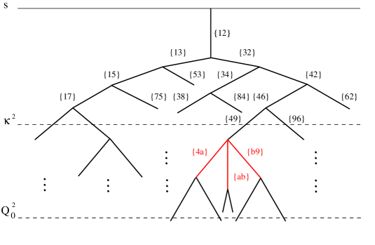
Figure 2: Example of an evolution tree of dipole $\{12\}$. Each edge in the graph corresponds to a dipole. The nodes correspond to an iteration of $Z^{(0)}[Q;\{u\}]$ except for the (red) node describing the splitting of dipole $\{49\}$ which indicates the double emission insertion in the r.h.s. of the evolution equation (46) for $Z^{(1)}[Q;\{u\}]$.

4 Perturbative solution of the evolution equations

In this section we discuss how Eq. (3) can be calculated using Monte Carlo methods. We will start with Sec. 4.1 by reporting the dipole-shower algorithm to solve the LL counter-part of Eq. (37), originally derived in Ref. Dasgupta:2001sh , then we move on to discuss the NLL corrections to the cumulative cross section (3) (or equivalently (3)), in configurations with three (Sec. 4.2) and two (Sec. 4.3) hard partons in the final state.

In the rest of this article, we also restore the full dependence on $N_{c}$ both in the QCD beta function used in the evolution of the running coupling (17) and in the cusp anomalous dimension (21). This by no means implies full control over finite-$N_{c}$ corrections, as additional subleading-$N_{c}$ terms are neglected in the evolution equations. We therefore replace Eq. (17) with the full RGE (notice that an overall factor $N_{c}/\pi$ is present in Eq. (17))

$$\frac{d\alpha_{s}(\mu)}{d\ln\mu^{2}}=-\beta(\alpha_{s})=-\alpha_{s}\left(\beta_{0}\alpha_{s}+\beta_{1}\alpha_{s}^{2}+\dots\right)\,,$$ (47)

with

$$\beta_{0}=\frac{11C_{A}-2n_{F}}{12\pi}\,,\quad\beta_{1}=\frac{17C_{A}^{2}-5C_{A}n_{F}-3C_{F}n_{F}}{24\pi^{2}}\,.$$ (48)

Moreover we replace in Eq. (37)

$$\bar{\alpha}(k_{ta})\bar{K}^{(1)}\to\frac{\alpha_{s}(k_{ta})}{2\pi}\,K^{(1)}\,,\quad K^{(1)}=\left(\frac{67}{18}-\frac{\pi^{2}}{6}\right)C_{A}-\frac{5}{9}n_{F}\,.$$ (49)

Similarly, we will retain the full colour quadratic $SU(N_{c})$ Casimir operators in the calculation of the hard coefficients ${\cal H}_{2}$ and ${\cal H}_{3}$ in Sec. 4.2 below.

4.1 LL evolution algorithm

At LL, Eq. (3) can be solved with the dipole shower algorithm derived in the pioneering article by Dasgupta and Salam Dasgupta:2001sh , that we adapt below to the problem considered here and to the case of dipole-transverse-momentum ordering. For later use, we define the evolution time

$$t\coloneqq\int_{\frac{k_{t}}{\sqrt{s}}}^{1}\frac{dx}{x}\bar{\alpha}(x\sqrt{s})=-\frac{N_{c}}{2\pi\beta_{0}}\ln\left(1-2\lambda\right)\,,\qquad\lambda=\beta_{0}\alpha_{s}(\sqrt{s})\ln\frac{\sqrt{s}}{k_{t}}\,.$$ (50)

The solution to Eq. (3) is then obtained with Algorithm 1, which is iterated until the desired statistical precision is reached. In the following, we define the infrared scale $Q_{0}$ as the singularity of Eq. (50), namely such that

$$2\,\beta_{0}\alpha_{s}(\sqrt{s})\ln\frac{\sqrt{s}}{Q_{0}}=1\,.$$ (51)

In practice, this scale is extremely low and therefore the evolution is rarely stopped because the scale $Q_{0}$ is reached before any emission is radiated into the interjet rapidity gap.

An important aspect to stress about Algorithm 1, is that at every step emissions are generated in the emitting dipole rest frame, but the observable is calculated in the event frame. We therefore need to apply a simple Lorentz transformation at every evolution step to transform the generated emission into the event frame. In doing this, we only need to keep track of the direction of the generated momenta, while the information regarding the dipole transverse momentum (i.e. the normalisation of the momenta) is encoded in the evolution time $t$. Therefore, we divide all momenta by their energy in the event frame, and keep track of the normalisation separately. As in Ref. Dasgupta:2001sh , all Lorentz transformation discussed in all algorithms presented in this section have to be performed with normalised momenta. This solves the problem of handling numerically Lorentz transformations involving very soft momenta. Also, it allows us to perform the evolution without any momentum conservation at any evolution step, thus eliminating exactly all subleading power (i.e. non-logarithmic) corrections.

Set $i=0$ and the evolution time $t_{0}=0$;

Start with one initial dipole made by the Born fermionic line;

while true do

       Compute $\Delta\eta_{\rm tot}=\sum_{\ell=1}^{N}\Delta\eta_{\ell}$, the sum of the available rapidity ranges within each of the $N$ dipoles in the event so far;

       Increase $i$ by 1;

       Generate a random number $r\in[0,1]$ & increase $t$ by an amount $\Delta t=t_{i}-t_{i-1}$ generated by solving

$$\frac{\Delta_{12}(k_{t,i-1})}{\Delta_{12}(k_{t,i})}=e^{-\Delta\eta_{\rm tot}\Delta t}=r\,;$$

Generate the dipole transverse momentum $k_{t,i}$ of the next emission $k_{i}$ by solving Eq. (50) with the new $t_{i}$. Generate its azimuth uniformly in $[0,2\pi]$ and its rapidity such that the emission is at a safety rapidity distance $\delta$ from the dipole extremities in the event frame;

       Choose the emitting dipole ${\cal D}_{\ell}$ with probability $\Delta\eta_{\ell}/\Delta\eta_{\rm tot}$;

       if $k_{t,i}<Q_{0}$ then

            break;

       end if

      Split the dipole ${\cal D}_{\ell}$ into two adjacent dipoles;

       if $\Theta_{\rm in}(k_{i})=1$ then

            Calculate observable and add the event to the histogram & break;

       end if

      

end while

Algorithm 1 LL evolution algorithm

We now discuss the calculation of the observable in a given event. The evolution in Algorithm 1 stops as soon as one gluon is emitted inside the interjet rapidity gap. We then calculate the transverse energy $E_{t}$ of this gluon w.r.t. the thrust axis of the event, and add the event to the histogram. We notice that in Ref. Dasgupta:2002bw , the transverse energy is instead defined as the value of the ordering variable. This definition is correct at LL, but the exact relation between the ordering variable and the actual observable leads to a genuine NLL effect. In this article we include these effects already in the LL prediction, and therefore we work with the physical observable everywhere in our calculation.

4.2 NLL evolution algorithm: ${\cal H}_{3}\otimes S_{3}(v)$ contribution

We now move on with the NLL corrections. We start from the ${\cal H}_{3}\otimes S_{3}(v)$ contribution to the cumulative cross section (3), which describes the production of three hard partons inside the jets (i.e. outside the interjet rapidity gap). The three partons can be viewed as two independent colour dipoles in a large-$N_{c}$ picture (in the case of $e^{+}e^{-}$ collisions), labelled as $\{13\}$ and $\{23\}$ in the second term of the r.h.s. of Eq. (3). These subsequently emit soft radiation independently of each other into the measured interjet region. The soft evolution of each of the above two dipoles, encoded in $S_{3}$, is carried out at LL order using Algorithm 1, and it is therefore straightforward. However, some care must be taken in the calculation of the hard factor ${\cal H}_{3}$ corresponding to the three hard-parton contribution. Specifically, in Ref. Banfi:2021owj as well as in Sec. 2 we have stated that the hard factors are individually IRC finite, while the integral over the three-parton final state clearly has divergences associated to singular kinematic configurations. At NLL, these divergence are meant to be cancelled by corresponding divergent contributions in the virtual corrections entering ${\cal H}_{2}$, and such a cancellation has to be enforced by means of a subtraction procedure. This also implies that the precise definition of the hard matching coefficients ${\cal H}_{2}$ and ${\cal H}_{3}$ depends on the scheme adopted to subtract their IRC divergences and only their combination has a physical meaning. In Section 5 of Ref. Banfi:2021owj the calculation was carried out analytically. However, in this article we would like to take a different approach and set up a numerical calculation using a local subtraction method that can be easily applied to the case of more complicated processes. As a consequence, the individual definition of ${\cal H}_{2}$ and ${\cal H}_{3}$ computed here will differ from those of Ref. Banfi:2021owj while their physical sum will be identical.

We start by labelling with $p_{1}$, $p_{2}$, $p_{3}$ the quark, antiquark and gluon respectively. With the usual $x_{1},x_{2},x_{3}$ variables

$$x_{i}=\frac{2(p_{i}\cdot q)}{s}\,,\quad i=1,2,3\,,\qquad x_{1}+x_{2}+x_{3}=2\,,$$ (52)

where $q$ is the four momentum of the virtual photon $q^{\mu}=(\sqrt{s},\vec{0})$. To obtain ${\cal H}_{3}\otimes S_{3}(v)$, we start by evaluating the integral over the $q\bar{q}g$ phase space. We choose the reference frame so that the $z$ axis is along the direction of the quark $\vec{p}_{1}$, and we explicitly parametrise the phase space of the remaining two partons in terms of the energy fraction of the gluon $x_{3}=2E_{g}/\sqrt{s}$ and the cosine of the angle between the gluon and the quark $y=\cos\theta_{qg}$. The real contribution to ${\cal H}_{3}\otimes S_{3}(v)$ is

$$\Sigma^{{\rm real}}(v) =2C_{F}\frac{\alpha_{s}}{2\pi}\left(\frac{\mu^{2}}{s}\right)^{\epsilon}\frac{e^{\gamma_{E}\epsilon}}{\Gamma(1-\epsilon)}\int_{0}^{1}dx_{3}\frac{x_{3}^{-1-2\epsilon}}{(1-x_{3})^{2\epsilon}}\int_{-1}^{1}dy\,\frac{(1-y)^{-1-\epsilon}(1+y)^{-1-\epsilon}}{(2-x_{3}(1-y))^{2-2\epsilon}}$$

$$\times\left(8-\epsilon x_{3}^{2}(2-x_{3}(1-y))^{2}-(2-x_{3})x_{3}\left((x_{3}-2)x_{3}(1-y)^{2}-4y+8\right)\right)$$

$$\times\Theta_{\rm out}(p_{1})\Theta_{\rm out}(p_{2})\Theta_{\rm out}(p_{3})\,S_{3}(v)\,,$$ (53)

where the coupling has been renormalised in the $\overline{\rm MS}$ scheme. The phase space constraint $\Theta_{\rm out}(p_{1})\Theta_{\rm out}(p_{2})\Theta_{\rm out}(p_{3})$ is non trivial, and imposes that none of the hard particles ends up inside the interjet rapidity gap, as per definition of ${\cal H}_{3}$. We stress that the direction of the thrust axis, that is used to define the position of the interjet rapidity gap, is now aligned with the hardest parton. For a given value of $x_{3}$ and $y$ the event is then dressed by a shower of soft gluons encoded in $S_{3}$, so that the integration over the remaining phase space of the three-parton system (specifically $y$) involves also the soft factor $S_{3}$. Eq. (4.2) produces double and single poles of soft and collinear origin, and we wish to perform a local subtraction of these divergences so that the above integral is computed numerically. We consider a simple subtraction scheme in which the local counter-term is defined by the full real integrand albeit with unresolved kinematics. That is, we build the counter-term by replacing the phase space constraint in Eq. (4.2) with

$$\Theta_{\rm out}(p_{1})\Theta_{\rm out}(p_{2})\Theta_{\rm out}(p_{3})\to\Theta_{\rm out}^{\rm soft}(p_{3})\,.$$ (54)

Here $\Theta_{\rm out}^{\rm soft}(p_{3})$ indicates that when the gluon $p_{3}$ is unresolved (i.e. either soft or collinear to either quark leg) the thrust axis is aligned along the $z$-axis and therefore $\Theta_{\rm out}(p_{1})=\Theta_{\rm out}(p_{2})=1$ by construction. The addition of such a counter-term modifies Eq. (4.2) as follows

$$\Sigma^{(3),{\rm sub}}(v) =2C_{F}\frac{\alpha_{s}}{2\pi}\left(\frac{\mu^{2}}{s}\right)^{\epsilon}\frac{e^{\gamma_{E}\epsilon}}{\Gamma(1-\epsilon)}\int_{0}^{1}dx_{3}\frac{x_{3}^{-1-2\epsilon}}{(1-x_{3})^{2\epsilon}}\int_{-1}^{1}dy\,\frac{(1-y)^{-1-\epsilon}(1+y)^{-1-\epsilon}}{(2-x_{3}(1-y))^{2-2\epsilon}}$$

$$\times\left(8-\epsilon x_{3}^{2}(2-x_{3}(1-y))^{2}-(2-x_{3})x_{3}\left((x_{3}-2)x_{3}(1-y)^{2}-4y+8\right)\right)$$

$$\times\left[\Theta_{\rm out}(p_{1})\Theta_{\rm out}(p_{2})\Theta_{\rm out}(p_{3})\,S_{3}(v)-\Theta_{\rm out}^{\rm soft}(p_{3})\,S_{2}(v)\right]\,,$$ (55)

where $S_{2}$ in the last term indicates that the soft factor now does not see the unresolved gluon $p_{3}$ and therefore it degenerates into the two-leg factor $S_{2}$. We point out that this procedure is a simple adaptation of the projection-to-Born subtraction method Cacciari:2015jma to an all-order calculation, where the projection acts on the full real phase space including the soft factor $S_{3}$. Eq. (4.2) is free of collinear singularities, however it still contains a soft singularity due to the fact that $S_{3}(v)$ depends on the direction of $p_{3}$ regardless of how soft the latter is. We then introduce a technical cutoff on the transverse momentum of the gluon $p_{3}$ w.r.t. the $\{12\}$ dipole ($p_{t,3}^{\{12\}}>Q_{0}$), and we set $\epsilon\to 0$ and evaluate the integral with Algorithm 2 (again iterated until the desired statistical precision is reached).

Generate $x_{3}$ and $y$ and parametrise the kinematics of the $q\bar{q}g$ system in terms of these variables;

if $p_{t,3}^{\{12\}}<Q_{0}$ then

      break and generate a new event;

end if

Set the weight $w$ to the integrand in the first two lines of Eq. (4.2) with $\epsilon=0$;

Create an event:

while true do

       Set the thrust axis along the direction of the hardest parton;

       if $\Theta_{\rm out}(p_{1})\Theta_{\rm out}(p_{2})\Theta_{\rm out}(p_{3})=0$ then

            break;

       end if

      Consider the two large-$N_{c}$ dipoles $\{13\}$ and $\{23\}$ and apply the LL evolution algorithm 1 to compute the soft factor $S_{3}$ at leading colour;

       break;

      

end while

Create a counter-event:

Set $w\mathrel{*}=-1$;

while true do

       Set the thrust axis along the direction of the quark ($z$ direction);

       if $\Theta_{\rm out}^{\rm soft}(p_{3})=0$ then

            break;

       end if

      Consider the dipole $\{12\}$ and apply the LL evolution algorithm 1 to compute the soft factor $S_{2}$ while filling the same histogram as for the event;

       break;

      

end while

Algorithm 2 NLL evolution algorithm for ${\cal H}_{3}\otimes S_{3}(v)$

The computation of Eq. (4.2) does not directly return the contribution ${\cal H}_{3}\otimes S_{3}(v)$. This is obtained by subtracting the double counting with the term ${\cal H}_{2}\otimes S_{2}(v)$, where the first gluon $p_{3}$ is now generated according to the LL evolution kernel. This requires subtracting from Eq. (4.2) the term Banfi:2021owj (we set $N_{c}\rightarrow 2C_{F}$ for this first emission)

$$\Sigma^{(3),{\rm sub}}_{\rm soft}(v) =4C_{F}\frac{\alpha_{s}}{2\pi}\mu^{2\epsilon}\frac{e^{\gamma_{E}\epsilon}}{\Gamma(1-\epsilon)}\int_{0}^{\sqrt{s}}\frac{dk_{t}}{k_{t}^{1+2\epsilon}}\int_{\ln(k_{t}/\sqrt{s})}^{\ln(\sqrt{s}/k_{t})}\,d\eta\,\Theta^{\rm soft}_{\rm out}(k)\left[S^{\rm soft}_{3}(v)-S_{2}(v)\right]\,,$$ (56)

where $S^{\rm soft}_{3}$ indicates that the emission of the soft gluon $k$ does not cause any recoil in the $q\bar{q}g$ event kinematics, and therefore the thrust axis is always aligned with the $z$-axis. In Eq. (56) we have adopted the same subtraction method used in Eq. (4.2), thereby subtracting the local counter-term evaluated in the unresolved (i.e. two-leg) kinematics. Eq. (56) also contains the soft singularity present in Eq. (4.2), and therefore we need to apply the same technical cutoff $k_{t}>Q_{0}$ here. It is now crucial to notice that the difference between the two equations is instead finite in the limit $Q_{0}\to 0$, and the regulator can be pushed to negligibly small values in the combination of the two. Eq. (56) can be evaluated with a slightly modified version of Algorithm 2, given in Algorithm 3.

Generate $\vec{k}_{t}$ and $\eta$ of the gluon $k$ and the back-to-back $q\bar{q}$ pair along the $z$ axis;

if $k_{t}<Q_{0}$ then

      break and generate a new event;

end if

Set the weight $w$ to the integrand in Eq. (56) with $\epsilon=0$ (w/o $\Theta$ and $S_{n}$ factors);

Set the thrust axis along the direction of the quark ($z$ direction);

Create an event:

while true do

       if $\Theta_{\rm out}^{\rm soft}(k)=0$ then

            break;

       end if

      Consider the two large-$N_{c}$ dipoles $\{13\}$ and $\{23\}$ and apply the LL evolution algorithm 1 to compute the soft factor $S^{\rm soft}_{3}$ at leading-colour;

       break;

      

end while

Create a counter-event:

Set $w\mathrel{*}=-1$;

while true do

       if $\Theta_{\rm out}^{\rm soft}(k)=0$ then

            break;

       end if

      Consider the dipole $\{12\}$ and apply the LL evolution algorithm 1 to compute the soft factor $S_{2}$ while filling the same histogram as for the event;

       break;

      

end while

Algorithm 3 NLL evolution algorithm for the soft contribution to ${\cal H}_{3}\otimes S_{3}(v)$

Finally we obtain ${\cal H}_{3}\otimes S_{3}(v)$ as the difference between the two contributions

$${\cal H}_{3}\otimes S_{3}(v)=\Sigma^{(3),{\rm sub}}(v)-\Sigma^{(3),{\rm sub}}_{\rm soft}(v)\,.$$ (57)

The above procedure used to define ${\cal H}_{3}$ implicitly also defines uniquely the two-parton hard coefficient ${\cal H}_{2}$. This will be given by the one loop correction to the quark form factor minus the integrals of the local counter-terms appearing in Eq. (57), minus the virtual correction to the evolution kernel that is subtracted to avoid the double counting with $S_{2}$ (see Section 5 of Ref. Banfi:2021owj ). The latter contribution to ${\cal H}_{2}\otimes S_{2}(v)$ reads Banfi:2021owj

$$\Sigma^{(2),{\rm virt.}}_{\rm soft}(v) =4C_{F}\frac{\alpha_{s}}{2\pi}\mu^{2\epsilon}\frac{e^{\gamma_{E}\epsilon}}{\Gamma(1-\epsilon)}\int_{0}^{\sqrt{s}}\frac{dk_{t}}{k_{t}^{1+2\epsilon}}\int_{\ln(k_{t}/\sqrt{s})}^{\ln(\sqrt{s}/k_{t})}d\eta\,S_{2}(v)\,.$$ (58)

This yields

$${\cal H}_{2} =\delta^{(2)}(\Omega_{1}-\Omega_{q})\delta^{(2)}(\Omega_{2}-\Omega_{\bar{q}})\left(1\!+\!\frac{\alpha_{s}}{2\pi}{\cal H}_{2}^{(1)}+{\cal O}(\alpha_{s}^{2})\right)\,,$$ (59)

where

$${\cal H} {}_{2}^{(1)}=\frac{C_{F}}{2\left(1-c^{2}\right)^{2}}\bigg{(}4\left(1-c^{2}\right)^{2}\left(\text{Li}_{2}\left(\frac{1+c}{2}\right)\!-\!\text{Li}_{2}\left(\frac{1-c}{2}\right)\right)$$

$$-2\left(1-c^{2}\right)^{2}\log^{2}(1+c)+16c\left(3+c^{2}\right)\ln(2)-(1-c^{2})(c(16+3c)-3)$$

$$+2\ln(1-c)\left(-2\left(1+c^{4}\right)\log(2)-4c\left(3+c^{2}\right)+\left(1-c^{2}\right)^{2}\ln(1-c)\right)$$ (60)

$$+\left(4\left(1+c^{4}\right)\ln(2)-8c\left(3+c^{2}\right)\right)\ln(1+c)-4\left(-3c^{4}+2c^{2}(9+2\ln(2))+1\right)\tanh^{-1}(c)\bigg{)}\,.$$

Here $c$ is the cosine of the jet opening angle, defined in Eq. (1). This coefficient will be used in the next section for the calculation of the ${\cal H}_{2}\otimes S_{2}(v)$ contribution to the NLL cumulative cross section.

4.3 NLL evolution algorithm: ${\cal H}_{2}\otimes S_{2}(v)$ contribution

We now address the numerical solution to the evolution equations (3), (46). We start by considering the contribution $Z^{(0)}_{12}[Q;\{u\}]$, defined by the evolution equation (3). The solution to Eq. (3) can be obtained with proper modifications of Algorithm 1. However, while Algorithm 1 can be used to calculate $Z^{(0)}_{12}[Q;\{u\}]$, defined by Eq. (3), in order to include the contribution from $Z^{(1)}_{12}[Q;\{u\}]$ given in Eq. (46) we cannot simply run Algorithm 1 down to the infrared scale $Q_{0}$. Instead, we first introduce a truncated version of Algorithm 1, given in Algorithm 4.

Set the thrust axis along the $z$ axis;

Generate the truncation scale $\kappa\in[Q_{0},\sqrt{s}]$ uniformly according to eq. (62);

Set the weight $w={\cal H}_{2}$ as defined in Eq. (59);

Apply Algorithm 1 with evolution time (4.3) truncated at $Q_{0}=\kappa$;

Algorithm 4 Truncated NLL algorithm for the first evolution branch

Firstly, we replace the evolution time (50) by its NLL counterpart

$$t\coloneqq \int_{\frac{k_{t}}{\sqrt{s}}}^{1}\frac{dx}{x}\bar{\alpha}(x\sqrt{s})\bigg{(}1+\frac{\alpha_{s}(x\sqrt{s})}{2\pi}\,K^{(1)}\bigg{)}=-\frac{N_{c}}{2\pi\beta_{0}}\ln\left(1-2\lambda\right)$$

$$+\bar{\alpha}(\sqrt{s})\left[\frac{\lambda}{1-2\lambda}\left(\frac{K^{(1)}}{2\pi\beta_{0}}-\frac{\beta_{1}}{\beta_{0}^{2}}\right)-\frac{\ln(1-2\lambda)}{1-2\lambda}\frac{\beta_{1}}{2\beta_{0}^{2}}\right]+{\cal O}({\rm NNLL})\,.$$ (61)

The above equation uniquely defines the dipole transverse momentum given the evolution time for a given emission. We now introduce the scale $\kappa$ at which we truncate a first branch of the evolution carried out according to the equation (3). The rationale is to use the simple partition of unity in the evolution sequence

$$1=\int_{Q_{0}}^{\sqrt{s}}\frac{d\kappa}{\sqrt{s}-Q_{0}}\,,$$ (62)

and use the fact that the evolution (3) between $\sqrt{s}$ and $Q_{0}$ is identical to the combination of the evolution between $\sqrt{s}$ and $\kappa$, and the evolution between $\kappa$ and $Q_{0}$. For each value of the scale $\kappa$ we will insert either one or two emissions, to perform a calculation of Eqs. (3), (46). These are identified by the three contributions defined below. According to Eq. (62) this scale is sampled uniformly and ensures that each insertion can occur at any possible scale along the evolution tree.

Generate emission $k_{a}$ according to Algorithm 6 and split the emitting dipole;

Apply Algorithm 1 with starting scale $k_{ta}$ and evolution time (4.3);

Algorithm 5 Insertion of $Z^{(0)}_{12}[Q;\{u\}]$ starting from the scale $\kappa$

To carry on with the calculation of $Z^{(0)}_{12}[Q;\{u\}]$ starting from Algorithm 4, we simply generate an emission $k_{a}$ according to Eq. (3) and then continue with the evolution from the scale of the emission all the way down to $Q_{0}$. This procedure is described in Algorithm 5.

Select an emitting dipole $\{p_{\ell_{1}}p_{\ell_{2}}\}$ for $k_{a}$ as in Algorithm 1;

Generate $k_{ta}$ as in Algorithm 1, starting from the scale $\kappa$;

Algorithm 6 Generation of emission $k_{a}$ starting from the scale $\kappa$

Let us now move to Eq. (46). We calculate separately the contributions proportional to $\tilde{w}_{12}^{(0)}$ and the strongly-ordered squared amplitude in Eq. (46), starting with the former. Its calculation is addressed by Algorithm 7, that we now outline. We start with the truncated evolution introduced above, and starting from the truncation scale $\kappa$ we generate two insertions of momenta $k_{a}$ and $k_{b}$. We start by considering the two ratios of Sudakov factors $\Delta_{12}(Q)/\Delta_{12}(k_{t(ab)})$ and $\Delta_{12}(Q)/\Delta_{12}(k_{ta})$ in the second and third term in the r.h.s. of Eq. (46), respectively. As shown in Ref. Banfi:2021owj , these two terms only contribute at NLL in the unordered kinematic region where $k_{ta}\sim k_{tb}^{\prime}\sim k_{tb}$, while they cancel in strongly ordered regimes. We can therefore introduce an extra ratio of Sudakov factors between the scales $k_{ta}$ and $k_{tb}$ in the second and third terms in the r.h.s. of Eq. (46), as it only amounts to introducing subleading logarithmic corrections since 

$${\cal O}\left(\alpha_{s}\ln\frac{k_{ta}}{k_{t(ab)}}\right)\sim{\cal O}\left(\alpha_{s}\ln\frac{k_{ta}}{k_{tb}}\right)\sim{\cal O}\left(\alpha_{s}\right)\,.$$ (63)

Concretely, for the contributions in which $k_{b}$ is emitted off dipole $\{1a\}$ we can make the replacements

$$\bar{\alpha}^{2}(k_{t(ab)})\frac{\Delta_{12}(Q)}{\Delta_{12}(k_{t(ab)})} \rightarrow\bar{\alpha}(k_{ta})\bar{\alpha}(k_{tb})\frac{\Delta_{12}(Q)}{\Delta_{12}(k_{ta})}\frac{\Delta_{1a}(k_{ta}\,k_{tb}/k_{tb}^{\prime})}{\Delta_{1a}(k_{tb})}\,,$$ (64)

$$\bar{\alpha}^{2}(k_{ta})\frac{\Delta_{12}(Q)}{\Delta_{12}(k_{ta})} \rightarrow\bar{\alpha}(k_{ta})\bar{\alpha}(k_{tb})\frac{\Delta_{12}(Q)}{\Delta_{12}(k_{ta})}\frac{\Delta_{1a}(k_{ta})}{\Delta_{1a}(k_{tb})}\,,$$ (65)

in the second and third term in the r.h.s. of Eq. (46), respectively. The complementary colour flow (i.e. $k_{b}$ is emitted off dipole $\{a2\}$) is treated analogously. These approximations are unnecessary from a purely theoretical point of view (they introduce at most NNLL corrections). However, the extra ratio of Sudakov factors has the advantage of suppressing regions of phase space close to the collinear singularity, therefore guaranteeing a much improved numerical stability in the calculation. Following exactly the same reasoning, we can also replace $k_{t(ab)}$ with $k_{ta}$ in the scale of all the $Z^{(0)}$ generating functionals in the second term in the r.h.s. of Eq. (46). This also preserves the collinear safety of the latter.

Generate emissions $k_{a}$ and $k_{b}$ according to Algorithms 6 and 8, respectively;

Create an event:

while true do

       if $\Theta_{\rm in}(k_{a})=1$ and $\Theta_{\rm in}(k_{b})=1$ then

             Reconstruct $k_{(ab)}$ with Eq. (26);

             Fill the histogram with $V(k_{(ab)})$ iff $\Theta_{\rm in}(k_{(ab)})=1$ and break;

       else if $\Theta_{\rm in}(k_{a})=1$ or $\Theta_{\rm in}(k_{b})=1$ then

             Fill the histogram with either $V(k_{a})$ or $V(k_{b})$ and break;

       end if

      Split the emitting dipole into three adjacent dipoles according to $k_{a}$ and $k_{b}$;

       Apply Algorithm 1 with starting scale $k_{ta}$ and evolution time (4.3);

       break;

      

end while

Create a counter-event:

Set $w\mathrel{*}=-1$;

while true do

       Reconstruct $k_{(ab)}$ with Eq. (26);

       Replace $k_{a}$ with $k_{(ab)}$;

       if $\Theta_{\rm in}(k_{(ab)})=1$ then

            Fill the histogram with $V(k_{(ab)})$ and break;

       end if

      Split the emitting dipole into two adjacent dipoles according to $k_{(ab)}$;

       Apply Algorithm 1 with starting scale $k_{ta}$ and evolution time (4.3);

       break;

      

end while

Algorithm 7 Insertion of $Z^{(1)}_{12}[Q;\{u\}]$ starting from the scale $\kappa$

In Eq. (64), the argument of the second Sudakov is such that we can generate

$$k_{tb}\leq k_{ta}\frac{k_{tb}}{k_{tb}^{\prime}}=k_{ta}\,f(p_{\ell_{1}},p_{\ell_{2}},\hat{k}_{b})\,,$$ (66)

where we used

$$k_{tb}^{\prime}=\frac{k_{tb}}{f(p_{\ell_{1}},p_{\ell_{2}},\hat{k}_{b})}\,.$$ (67)

The function $f(p_{\ell_{1}},p_{\ell_{2}},\hat{k}_{b})$, defined in Eq. (68), exclusively depends on the directions of the momenta $p_{\ell_{1}}$, $p_{\ell_{2}}$, $k_{b}$ and not on their energies. Eq. (66) arises from requiring $k_{tb}^{\prime}<k_{ta}$. The first ($k_{a}$) and second ($k_{b}$) insertions are then generated according to Algorithms 6 and 8, respectively.

We then calculate the difference of terms proportional to $\tilde{w}_{12}^{(0)}$ in Eq. (46). An important remark concerns the construction of the $k_{(ab)}$ momentum appearing in the counter-term in Eq. (46). This momentum is introduced in Eq. (26) where it is defined in the rest frame of the dipole that radiates the pair $k_{a}$, $k_{b}$ (with dipole axis along the $z$ direction), and needs to be Lorentz transformed back into the event frame. All Lorentz transformations are performed as described in Sec. 4.1, using momenta with unit energy. A last comment about the procedure to fill the histograms in Algorithm 7 is in order. In particular, in order to eliminate NNLL contributions, when both insertions $k_{a}$ and $k_{b}$ are in the interjet rapidity gap in the event we consider the observable calculated on the massless parent defined in Eq. (26). This procedure exactly reproduces what is done in the counter-event, and therefore ensures that for the NNLL configurations in which both insertions are in the gap the two contributions cancel by construction.

Finally, the remaining contribution to the evolution (46) of $Z^{(1)}_{12}[Q;\{u\}]$, proportional to the strongly ordered double-soft squared amplitude ($w^{(0)}_{12}w^{(0)}_{a2}$ and $w^{(0)}_{12}w^{(0)}_{1a}$), is also obtained with Algorithm 7. Here one must replace all instances of $k_{(ab)}$ with $k_{a}$, and generate $k_{b}$ with the simpler constraint $k_{tb}<k_{ta}$, which is obtained by setting the angular function $f(p_{\ell_{1}},p_{\ell_{2}},\hat{k}_{b})\to 1$ in Eq. (68). Moreover, we set the weight according to the strongly-ordered limit of Eq. (69) (cf. Eq. (46)), that simply amounts to removing the reweighing step (69) altogether. This guarantees that the iteration of the LL evolution kernel in (3) is correctly subtracted. The final result for ${\cal H}_{2}\otimes S_{2}(v)$ is then obtained as the sum of the result of the above three contributions.

Pick the dipole that emits $k_{b}$ among $\{p_{\ell_{1}}k_{a}\}$ and $\{k_{a}p_{\ell_{2}}\}$ with probability $1/2$;

Update weight $w\mathrel{*}=2$;

Generate $k_{tb}$ w.r.t. the emitting dipole as in Algorithm 1 starting from the scale

$$k_{ta}\,f(p_{\ell_{1}},p_{\ell_{2}},\hat{k}_{b})\,,\quad f(p_{\ell_{1}},p_{\ell_{2}},\hat{k}_{b})\coloneqq\sqrt{\frac{(p_{\ell_{1}}\cdot p_{\ell_{2}})}{2(p_{\ell_{1}}\cdot\hat{k}_{b})(\hat{k}_{b}\cdot p_{\ell_{2}})}}\,,$$ (68)

where $\hat{k}_{b}$ denotes $k_{b}$ with its $k_{t}$ w.r.t. the emitting dipole set to one;

Update the weight

$$w\mathrel{*}=\frac{\tilde{w}^{(0)}_{12}(k_{b},k_{a})}{w^{(0)}_{12}(k_{a})w^{(0)}_{1a}(k_{b})}\,;\quad w\mathrel{*}=\frac{\tilde{w}^{(0)}_{12}(k_{a},k_{b})}{w^{(0)}_{12}(k_{a})w^{(0)}_{a2}(k_{b})}\,,$$ (69)

for the two dipoles, respectively;

Algorithm 8 Generation of emission $k_{b}$ starting from the scale $k_{ta}$

5 Numerical results for the $E_{t}$ distribution in the interjet gap at NLL

In this section we apply the technique described in Sec. 4 to the calculation of the transverse energy distribution in the rapidity gap between the two cone jets in $e^{+}e^{-}$. In the following we set $\sqrt{s}=M_{Z}$ and adopt the value $\alpha_{s}(M_{Z})=0.118$ for the strong coupling constant. To obtain a physical prediction for this observable, we introduce the standard perturbative scales used in resummed calculations whose variation quantifies the size of subleading logarithmic corrections. These are discussed in Appendix B. We vary the renormalisation scale $\mu_{R}$ by a factor of two around its central value $\mu_{R}=\sqrt{s}$, and for central $\mu_{R}$, we also vary the resummation scale $\mu_{Q}$ by a factor of two around its central value $\mu_{Q}=\sqrt{s}/2$. The final perturbative uncertainty shown in the results that follow is obtained as the envelope of the above five predictions. The calculation performed in this section is strictly speaking valid only in the limit of soft radiation, and therefore should be consistently matched to a fixed order calculation in the bulk of the phase space where the emitted radiation is hard. A matching of this type is standard in resummed calculation and must be performed in future phenomenological applications.

As a check of our calculation, we have also computed the LL $\Sigma(v)$ cumulative distribution as a function of the evolution variable $t$ defined in Eq. (50), and reproduced the results of Ref. Dasgupta:2002bw . Notice that the LL evolution time (50) is defined in terms of the dipole transverse momentum of the gluon that is radiated inside the interjet rapidity gap. This transverse momentum is related to the physical observable $E_{t}$ via an ${\cal O}(1)$ angular function that depends on the orientation of the emitting dipole w.r.t. the thrust axis, that varies on an event-by-event basis. Therefore the relation between $t$ and $E_{t}$ is not bijective. In Ref. Banfi:2021owj we have also compared the ${\cal O}(\alpha_{s}^{2})$ expansion of our calculation to fixed-order predictions in full QCD, finding excellent agreement in the limit of $E_{t}\to 0$. In the same article, we have also verified that our fixed-order expansion for the energy distribution $E$ reproduces the calculation of Ref. Becher:2016mmh . As a further check, we have carried out two independent implementations of the algorithms given in Sec. 4 and found complete agreement. A public version of the code can be found in Ref. gnole .

In the left plots of Figs. 3, 4, 5, we report the cumulative distribution (2) at LL and NLL for three different values for the width of the interjet rapidity gap ($\cos\theta_{\rm jet}=c=\{0.2,0.5,0.9\}$), which correspond to different opening angles of the two hard jets (cf. Eq. (1)). We observe that the definition of the infrared scale $Q_{0}$ in Eq. (51) (introduced in our prescription to deal with the Landau singularity in Eq. (31)) acts as a cutoff on the transverse momentum of the emissions w.r.t. the emitting dipole. Therefore, the region of the plots in which the observable $E_{t}\sim Q_{0}$ (and below) is susceptible to non-perturbative effects. We therefore truncate the plots at this scale (i.e. $\ln\sqrt{s}/E_{t}=1/(2\alpha_{s}\beta_{0})\simeq 7$) cutting out the non-perturbative region. We start by considering the region of the plots that corresponds to a large transverse energy inside the interjet rapidity gap. The predictivity here is restored upon a matching to a fixed-order calculation, which however is not performed in Figs. 3, 4, 5. We therefore do not comment further on this region and we rather focus on the small $E_{t}$ regime, where (non-global) resummation effects are dominant. We notice, however, that the normalisation of the curves at large $E_{t}$ changes with the size of the cone jets. This can understood by observing the $c$-dependence of the hard factors ${\cal H}_{2}$ and ${\cal H}_{3}$ calculated in Sec. 4. The residual scale dependence at large $E_{t}$ present at NLL is due to the $\mu_{R}$ dependence of the hard factors, which is absent by construction at LL. At small $E_{t}$, we observe that NLL corrections are large and negative, and reach $40\%$ in size when the resummed logarithms are large, consistently across different values of the jet cone size. We stress that the results presented here adopt the physical $E_{t}$ definition for the LL calculation rather than its strict leading-logarithmic limit in which $E_{t}$ is simply the dipole tranverse momentum of the emission in the interjet gap. In the latter case, the size of the genuine NLL corrections would be even larger as these would also compensate for the kinematical difference between the dipole $k_{t}$ and the actual definition of $E_{t}$. We also observe a substantial reduction of the perturbative uncertainty, up to a factor of two, in the NLL calculation compared to the LL prediction, whose uncertainty band however accounts for the large NLL corrections.

It is informative to study the size of the various contributions to the NLL corrections to the cumulative distribution. In the right plots of Figs. 3, 4, 5, we then show the breakdown of the NLL correction into three different pieces. These are the ${\cal H}_{n}\otimes S_{n}(v)$ terms in Eq. (3), with $n=2$ and $n=3$. Moreover, for $n=2$, we plot separately the contribution from the functional $Z_{12}^{(0)}$, defined in Eq. (3), and $Z^{(1)}_{12}$, defined in Eq. (46). We observe that for small interjet gaps, i.e. fat cone jets, the NLL result is completely dominated by the $Z_{12}^{(0)}$ correction, with an additional sizeable correction from the ${\cal H}_{3}\otimes S_{3}(v)$ term. For larger $c$ values (corresponding to narrower jets), however, the contribution of the $Z^{(1)}_{12}$ correction slightly grows and becomes comparable to that of the ${\cal H}_{3}\otimes S_{3}(v)$ term at small values of $E_{t}$. The moderate contribution of the $Z^{(1)}_{12}$ correction compared to $Z^{(0)}_{12}$ justifies entirely the perturbative approach adopted in Eq. (44) for the generating functional $Z_{12}$ which led to the evolution equations (3) and (46).

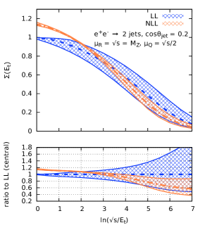
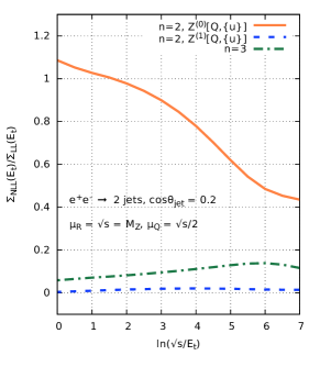
Figure 3: Left: cumulative distribution $\Sigma(E_{t})$ for the transverse energy in the interjet rapidity gap at LL and NLL for $c=0.2$. Right: breakdown of the contributions to the NLL correction, relative to the LL prediction.

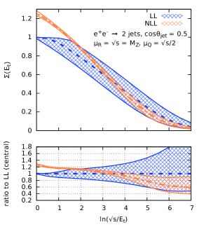
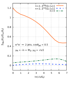
Figure 4: Left: cumulative distribution $\Sigma(E_{t})$ for the transverse energy in the interjet rapidity gap at LL and NLL for $c=0.5$. Right: breakdown of the contributions to the NLL correction, relative to the LL prediction.

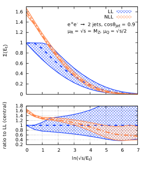
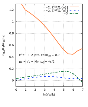
Figure 5: Left: cumulative distribution $\Sigma(E_{t})$ for the transverse energy in the interjet rapidity gap at LL and NLL for $c=0.9$. Right: breakdown of the contributions to the NLL correction, relative to the LL prediction.

6 Conclusions

In this article we have presented the first NLL resummation for non-global radiative corrections to a collider observable in the large-$N_{c}$ limit. We considered a set of evolution equations that we derived in a recent article, describing the dynamics of soft gluons emitted at large angles with respect to the hard scattering process. To solve these equations numerically, we have reformulated the resummation in terms of generating functionals, which can be used for the calculation of the emission probability associated with any given final state containing $n$ soft gluons. This formulation is suitable for a numerical implementation by means of Monte Carlo methods. Using this technology, we have presented an algorithm for the solution of the evolution equations, hence achieving the resummation of NLL non-global corrections. We applied this formalism to the calculation of the NLL distribution of the transverse energy $E_{t}$ of the radiation within the gap between two hard cone jets produced in $e^{+}e^{-}$ collisions. We found that the NLL corrections are rather sizeable and their inclusion leads to a substantial reduction of the perturbative scale uncertainties in the theoretical calculation. They do therefore play an important role in the accurate prediction of this class of observables at particle colliders.

We point out that the algorithms presented in this article are not tailored to the specific observable considered here, and are directly applicable to hadron-collider observables in the large-$N_{c}$ approximation. This is because the only process dependence occurs in the hard factors ${\cal H}_{n}$ of Eq. (3) (which in turn can be calculated algorithmically for a given process), while the evolution of the soft factors $S_{n}$ with the energy scale is entirely process independent as expected from the factorisation of squared amplitudes in the soft limit. Therefore, the formalism presented here can be applied to all observables that are solely sensitive to soft radiation emitted with large angles from the hard scattering, which are characterised by a single logarithmic perturbative expansion, i.e. the dominant logarithmic tower in the cumulative distribution is of the form $\alpha_{s}^{n}L^{n}$. The application to observables sensitive to collinear radiation, on the other hand, requires extra care since the formulation presented here must be supplemented with the correct resummation of the corresponding collinear logarithms (obtained for instance with standard techniques for global observables), and the double counting between the two regions (i.e. the soft and collinear limit) must be consistently subtracted in the evolution equations for the generating functionals. This subtraction is simple for most observables, and it simply amounts to dividing the cumulative distribution (3) by the contribution from primary radiation. This is obtained by running the algorithms given in Sec. 4 while forbidding the dipoles to split, so that all emissions are radiated off the primary $q\bar{q}$ dipole. However, we notice that there might be cases in which the subtraction becomes conceptually more delicate, such as in the case of observables affected by abelian clustering logarithms Banfi:2005gj . The technical details of these subtraction procedures, as well as the application to hadronic observables is left for future work.

The computer code Gnole gnole used to perform the calculations presented in this article can be downloaded from the repository:

https://github.com/non-global/gnole

Appendix A Symmetries of the squared amplitude and choice of ordering

In this appendix we comment on the choice of the dipole $k_{t}$ as ordering variable for the evolution equation. Let us start by considering the emission of two soft gluons in the strongly ordered limit, and we focus on the double-real integral

$$\frac{1}{2!}\int[dk_{a}]\int[dk_{b}]\left[w^{(0)}_{12}(k_{a})w^{(0)}_{1a}(k_{b})+w^{(0)}_{12}(k_{a})w^{(0)}_{a2}(k_{b})\right]u(k_{a})u(k_{b})\,.$$ (70)

We now introduce a partition of unity using the dipole transverse momentum

$$1=\Theta(k_{ta}-k_{tb})+\Theta(k_{tb}-k_{ta})\,.$$ (71)

We stress that the dipole $k_{tb}$ is defined differently in the two colour flow configurations of Eq. (70), following Eq. (28), which highlights the non-trivial nature of the partition (71). In order to write a Monte Carlo algorithm that iterates correctly the squared amplitude, the two regions in Eq. (71) must be identical (or at least in the kinematic limits relevant to a given logarithmic accuracy), so that the combinatorial factor $1/2!$ in Eq. (70) can be effectively replaced with a kinematic ordering. To show that dipole $k_{t}$ ordering is a suitable choice, we observe that the squared amplitude in the strongly-ordered limit satisfies the symmetry (e.g. in the case of two emissions)

$$\mathbb{T}\coloneqq\{\hat{n}_{a}\leftrightarrow\hat{n}_{b};k_{tb}\leftrightarrow k_{ta}\}\,,$$ (72)

where the transverse momenta are always meant w.r.t. the emitting dipole and the directions $\hat{n}_{a,b}$ are taken in the $\{12\}$ dipole frame. This symmetry is highly non trivial, and it is now interesting to understand how the integrand in Eq. (70) behaves under its action. We consider separately the two colour flows

$${\rm 1):}\quad\{1,a,b,2\}\,,\qquad{\rm 2):}\quad\{1,b,a,2\}\,,$$ (73)

and define the transformation $\mathbb{T}^{(i)}$ ($i=1,2$) such that for each colour flow we can obtain the transformed momenta $\tilde{k}_{a,b}$ as

$$\begin{bmatrix}\tilde{k}_{a}\\ \tilde{k}_{b}\end{bmatrix}=\mathbb{T}^{(i)}\begin{bmatrix}k_{a}\\ k_{b}\end{bmatrix}\,.$$ (74)

Imposing the constraints of Eq. (72) leads to

$$\mathbb{T}^{(1)}=\begin{bmatrix}0\qquad&\left(\frac{(p_{1}\cdot k_{b})(k_{a}\cdot p_{2})}{(p_{1}\cdot p_{2})(k_{a}\cdot k_{b})}\right)^{-1/2}\\ \left(\frac{(p_{1}\cdot k_{a})(k_{b}\cdot p_{2})}{(p_{1}\cdot p_{2})(k_{a}\cdot k_{b})}\right)^{1/2}\qquad&0\end{bmatrix}\,,$$ (75)

$$\mathbb{T}^{(2)}=\begin{bmatrix}0\qquad&\left(\frac{(p_{1}\cdot k_{a})(k_{b}\cdot p_{2})}{(p_{1}\cdot p_{2})(k_{a}\cdot k_{b})}\right)^{-1/2}\\ \left(\frac{(p_{1}\cdot k_{b})(k_{a}\cdot p_{2})}{(p_{1}\cdot p_{2})(k_{a}\cdot k_{b})}\right)^{1/2}\qquad&0\end{bmatrix}\,.$$ (76)

In the above matrices $\mathbb{T}^{(i)}$ each entry is to be understood to be proportional to the identity operator that acts on the four momenta as in Eq. (74). Let us also work out the action of the above transformation on the phase space measure. We find

$$\mathbb{T}^{(1)}\left[[dk_{a}][dk_{b}]\right]=\frac{(p_{1}\cdot k_{a})(k_{b}\cdot p_{2})}{(p_{1}\cdot k_{b})(p_{a}\cdot p_{2})}\,[dk_{a}][dk_{b}]\,,\,\,\,\mathbb{T}^{(2)}\left[[dk_{a}][dk_{b}]\right]=\frac{(p_{1}\cdot k_{b})(k_{a}\cdot p_{2})}{(p_{1}\cdot k_{a})(k_{b}\cdot p_{2})}\,[dk_{a}][dk_{b}]\,.$$ (77)

The strongly ordered squared amplitude is invariant under the above trasformations for each separate dipole, a consequence of the conformal symmetry of the integrand in the presence of strongly ordered kinematics. However, due to the non-trivial effect of $\mathbb{T}$ on the phase space measure, the LL integrand itself is not invariant. By applying the transformation to the integrand we find (e.g. for dipole $1$)

$$\mathbb{T}^{(1)}\left[[dk_{a}][dk_{b}]w^{(0)}_{12}(k_{a})w^{(0)}_{a2}(k_{b})\right]=[dk_{a}][dk_{b}]w^{(0)}_{12}(k_{a})w^{(0)}_{1a}(k_{b})\,,$$ (78)

that is the transformation simply maps the integrand into the one corresponding to the complementary colour configuration. This implies that the full LL integrand, given by the sum of the different dipoles is indeed invariant under $\mathbb{T}$, and that therefore the transverse momentum taken w.r.t. the emitting dipole can be adopted as an evolution variable as done in Eq. (12).

At NLL we need to consider unordered configurations in which the two emissions $k_{a}$ and $k_{b}$ are described by the full double-soft squared amplitude in large-$N_{c}$ $\tilde{w}^{(0)}_{12}(k_{a},k_{b})+\tilde{w}^{(0)}_{12}(k_{b},k_{a})$ (see Eq. (2)). This squared amplitude is not invariant under the $\mathbb{T}$ transformations, indicating that dipole $k_{t}$ ordering cannot be used for the calculation of the double-real correction (22). Instead, one can order the emissions $k_{a}$ and $k_{b}$ using their transverse momenta w.r.t. the $\{12\}$ dipole $k_{ta}$, $k_{tb}^{\prime}$, under which the squared amplitude is fully symmetric. This explains the factor $\Theta(k_{ta}-k_{tb}^{\prime})$ in Eq. (22). An alternative solution would be to formulate the whole evolution ordered in energy, which would allow one to use the same ordering in the strongly ordered limit as well as in unordered kinematic configurations.

Appendix B Dependence on the perturbative scales $\mu_{R}$ and $\mu_{Q}$

In this appendix we introduce the renormalisation $\mu_{R}$ and resummation $\mu_{Q}$ scales. In general, there are two sources of $\mu_{R}$ dependence, which appears both in the hard factors ${\cal H}_{2}$ and ${\cal H}_{3}$ as well as in the soft factors $S_{2}$ and $S_{3}$ (or equivalently in the generating functionals $Z_{12}[Q;\{u\}]$, $Z_{13}[Q;\{u\}]$ and $Z_{23}[Q;\{u\}]$ in Eq. (3)).

For the physical process under consideration, the $\mu_{R}$ dependence in the hard factors is entirely encoded in the $\overline{\rm MS}$ coupling

$$\alpha_{s}\to\alpha_{s}(\mu_{R})\,.$$ (79)

Extra dependence on $\mu_{R}$ in ${\cal H}_{2}$ and ${\cal H}_{3}$ arises for processes which are mediated by QCD interactions at the Born level, such as jet production at hadron colliders. The second source of $\mu_{R}$ dependence is given by the generating functionals. This is introduced by expressing $\bar{\alpha}(k_{t})$ in terms of $\bar{\alpha}\left(\frac{\mu_{R}}{\sqrt{s}}k_{t}\right)$ in Eq. (37), and then expanding out the result in $\bar{\alpha}\left(\mu_{R}\right)$ at fixed $\bar{\alpha}\left(\mu_{R}\right)\ln\frac{\sqrt{s}}{k_{t}}\sim 1$. The running of the coupling must match the logarithmic order of the calculation, and therefore we use one-loop running at LL and two-loop running at NLL.

The resummation scale $\mu_{Q}$ is introduced to estimate the size of subleading logarithmic corrections. Its dependence is entirely encoded in the soft factors, and thus in the generating functional. The whole $\mu_{R}$ and $\mu_{Q}$ scale dependence can be easily encoded in the evolution algorithms presented in Sec. 3. Specifically, it amounts to replacing the evolution times (50) (4.3) with

$$t\rightarrow \,\tilde{t}\coloneqq-\frac{N_{c}}{2\pi\beta_{0}}\ln\left(1-2\tilde{\lambda}\right)\,,\qquad\tilde{\lambda}=\beta_{0}\alpha_{s}(\mu_{R})\ln\frac{\mu_{Q}}{k_{t}}\,,$$ (80)

$$t\rightarrow \,\tilde{t}\coloneqq-\frac{N_{c}}{2\pi\beta_{0}}\ln\left(1-2\tilde{\lambda}\right)+\bar{\alpha}(\mu_{R})\frac{\tilde{\lambda}}{1-2\tilde{\lambda}}\ln\frac{\mu_{R}^{2}}{\mu_{Q}^{2}}+\bar{\alpha}(\mu_{R})\ln\frac{\sqrt{s}}{\mu_{Q}}$$

$$+\bar{\alpha}(\mu_{R})\left[\frac{\tilde{\lambda}}{1-2\tilde{\lambda}}\left(\frac{K^{(1)}}{2\pi\beta_{0}}-\frac{\beta_{1}}{\beta_{0}^{2}}\right)-\frac{\ln(1-2\tilde{\lambda})}{1-2\tilde{\lambda}}\frac{\beta_{1}}{2\beta_{0}^{2}}\right]+{\cal O}({\rm NNLL})\,,$$ (81)

at LL and NLL, respectively. The definition of the infrared scale $Q_{0}$ given in Eq. (51) is also consistently modified as follows

$$2\,\beta_{0}\alpha_{s}(\mu_{R})\ln\frac{\mu_{Q}}{Q_{0}}=1\,.$$ (82)

References

- (1) M. Dasgupta and G. P. Salam, Resummation of nonglobal QCD observables, Phys. Lett. B 512 (2001) 323–330, [hep-ph/0104277].
- (2) M. Dasgupta and G. P. Salam, Accounting for coherence in interjet E(t) flow: A Case study, JHEP 03 (2002) 017, [hep-ph/0203009].
- (3) A. Banfi, G. Marchesini and G. Smye, Away from jet energy flow, JHEP 08 (2002) 006, [hep-ph/0206076].
- (4) Y. Hatta and T. Ueda, Resummation of non-global logarithms at finite , Nucl. Phys. B 874 (2013) 808–820, [1304.6930].
- (5) Y. Hagiwara, Y. Hatta and T. Ueda, Hemisphere jet mass distribution at finite , Phys. Lett. B 756 (2016) 254–258, [1507.07641].
- (6) Y. Hatta and T. Ueda, Non-global logarithms in hadron collisions at = 3, Nucl. Phys. B 962 (2021) 115273, [2011.04154].
- (7) J. R. Forshaw, A. Kyrieleis and M. H. Seymour, Super-leading logarithms in non-global observables in QCD, JHEP 08 (2006) 059, [hep-ph/0604094].
- (8) J. R. Forshaw, A. Kyrieleis and M. H. Seymour, Super-leading logarithms in non-global observables in QCD: Colour basis independent calculation, JHEP 09 (2008) 128, [0808.1269].
- (9) T. Becher, M. Neubert and D. Y. Shao, Resummation of Super-Leading Logarithms, 2107.01212.
- (10) T. Becher, M. Neubert, L. Rothen and D. Y. Shao, Effective Field Theory for Jet Processes, Phys. Rev. Lett. 116 (2016) 192001, [1508.06645].
- (11) T. Becher, M. Neubert, L. Rothen and D. Y. Shao, Factorization and Resummation for Jet Processes, JHEP 11 (2016) 019, [1605.02737].
- (12) S. Caron-Huot, Resummation of non-global logarithms and the BFKL equation, JHEP 03 (2018) 036, [1501.03754].
- (13) A. J. Larkoski, I. Moult and D. Neill, Non-Global Logarithms, Factorization, and the Soft Substructure of Jets, JHEP 09 (2015) 143, [1501.04596].
- (14) A. Banfi, F. A. Dreyer and P. F. Monni, Next-to-leading non-global logarithms in QCD, 2104.06416.
- (15) J. Forshaw, J. Keates and S. Marzani, Jet vetoing at the LHC, JHEP 07 (2009) 023, [0905.1350].
- (16) M. Rubin, Non-Global Logarithms in Filtered Jet Algorithms, JHEP 05 (2010) 005, [1002.4557].
- (17) A. Banfi, M. Dasgupta, K. Khelifa-Kerfa and S. Marzani, Non-global logarithms and jet algorithms in high-pT jet shapes, JHEP 08 (2010) 064, [1004.3483].
- (18) R. M. Duran Delgado, J. R. Forshaw, S. Marzani and M. H. Seymour, The dijet cross section with a jet veto, JHEP 08 (2011) 157, [1107.2084].
- (19) M. Dasgupta, K. Khelifa-Kerfa, S. Marzani and M. Spannowsky, On jet mass distributions in Z+jet and dijet processes at the LHC, JHEP 10 (2012) 126, [1207.1640].
- (20) M. D. Schwartz and H. X. Zhu, Nonglobal logarithms at three loops, four loops, five loops, and beyond, Phys. Rev. D 90 (2014) 065004, [1403.4949].
- (21) T. Becher, B. D. Pecjak and D. Y. Shao, Factorization for the light-jet mass and hemisphere soft function, JHEP 12 (2016) 018, [1610.01608].
- (22) D. Neill, The Asymptotic Form of Non-Global Logarithms, Black Disc Saturation, and Gluonic Deserts, JHEP 01 (2017) 109, [1610.02031].
- (23) S. Caron-Huot and M. Herranen, High-energy evolution to three loops, JHEP 02 (2018) 058, [1604.07417].
- (24) A. J. Larkoski, I. Moult and D. Neill, The Analytic Structure of Non-Global Logarithms: Convergence of the Dressed Gluon Expansion, JHEP 11 (2016) 089, [1609.04011].
- (25) T. Becher, R. Rahn and D. Y. Shao, Non-global and rapidity logarithms in narrow jet broadening, JHEP 10 (2017) 030, [1708.04516].
- (26) R. Ángeles Martínez, M. De Angelis, J. R. Forshaw, S. Plätzer and M. H. Seymour, Soft gluon evolution and non-global logarithms, JHEP 05 (2018) 044, [1802.08531].
- (27) M. Balsiger, T. Becher and D. Y. Shao, Non-global logarithms in jet and isolation cone cross sections, JHEP 08 (2018) 104, [1803.07045].
- (28) D. Neill, Non-Global and Clustering Effects for Groomed Multi-Prong Jet Shapes, JHEP 02 (2019) 114, [1808.04897].
- (29) M. Balsiger, T. Becher and D. Y. Shao, NLL′ resummation of jet mass, JHEP 04 (2019) 020, [1901.09038].
- (30) M. Balsiger, T. Becher and A. Ferroglia, Resummation of non-global logarithms in cross sections with massive particles, JHEP 09 (2020) 029, [2006.00014].
- (31) N. Ziani, K. Khelifa-Kerfa and Y. Delenda, Jet mass distribution in Higgs/vector boson + jet events at hadron colliders with clustering, Eur. Phys. J. C 81 (2021) 570, [2104.11060].
- (32) H. Weigert, Nonglobal jet evolution at finite N(c), Nucl. Phys. B 685 (2004) 321–350, [hep-ph/0312050].
- (33) Y. Hatta, Relating e+ e- annihilation to high energy scattering at weak and strong coupling, JHEP 11 (2008) 057, [0810.0889].
- (34) M. Dasgupta, F. A. Dreyer, K. Hamilton, P. F. Monni and G. P. Salam, Logarithmic accuracy of parton showers: a fixed-order study, JHEP 09 (2018) 033, [1805.09327].
- (35) G. Bewick, S. Ferrario Ravasio, P. Richardson and M. H. Seymour, Logarithmic accuracy of angular-ordered parton showers, JHEP 04 (2020) 019, [1904.11866].
- (36) M. Dasgupta, F. A. Dreyer, K. Hamilton, P. F. Monni, G. P. Salam and G. Soyez, Parton showers beyond leading logarithmic accuracy, Phys. Rev. Lett. 125 (2020) 052002, [2002.11114].
- (37) J. R. Forshaw, J. Holguin and S. Plätzer, Building a consistent parton shower, JHEP 09 (2020) 014, [2003.06400].
- (38) S. Plätzer and I. Ruffa, Towards Colour Flow Evolution at Two Loops, 2012.15215.
- (39) K. Hamilton, R. Medves, G. P. Salam, L. Scyboz and G. Soyez, Colour and logarithmic accuracy in final-state parton showers, 2011.10054.
- (40) Z. Nagy and D. E. Soper, Summations of large logarithms by parton showers, 2011.04773.
- (41) Z. Nagy and D. E. Soper, Summations by parton showers of large logarithms in electron-positron annihilation, 2011.04777.
- (42) A. Karlberg, G. P. Salam, L. Scyboz and R. Verheyen, Spin correlations in final-state parton showers and jet observables, 2103.16526.
- (43) F. Dulat, S. Höche and S. Prestel, Leading-Color Fully Differential Two-Loop Soft Corrections to QCD Dipole Showers, Phys. Rev. D 98 (2018) 074013, [1805.03757].
- (44) L. Gellersen, S. Höche and S. Prestel, Disentangling soft and collinear effects in QCD parton showers, 2110.05964.
- (45) K. Hamilton, A. Karlberg, G. P. Salam, L. Scyboz and R. Verheyen, Soft spin correlations in final-state parton showers, 2111.01161.
- (46) K. Konishi, A. Ukawa and G. Veneziano, Jet Calculus: A Simple Algorithm for Resolving QCD Jets, Nucl. Phys. B 157 (1979) 45–107.
- (47) A. Bassetto, M. Ciafaloni and G. Marchesini, Jet Structure and Infrared Sensitive Quantities in Perturbative QCD, Phys. Rept. 100 (1983) 201–272.
- (48) Y. L. Dokshitzer, V. A. Khoze, A. H. Mueller and S. I. Troian, Basics of perturbative QCD. 1991.
- (49) J. M. Campbell and E. W. N. Glover, Double unresolved approximations to multiparton scattering amplitudes, Nucl. Phys. B 527 (1998) 264–288, [hep-ph/9710255].
- (50) A. Gehrmann-De Ridder, T. Gehrmann and E. Glover, Antenna subtraction at NNLO, JHEP 09 (2005) 056, [hep-ph/0505111].
- (51) A. Banfi, P. F. Monni, G. P. Salam and G. Zanderighi, Higgs and Z-boson production with a jet veto, Phys. Rev. Lett. 109 (2012) 202001, [1206.4998].
- (52) A. Banfi, H. McAslan, P. F. Monni and G. Zanderighi, A general method for the resummation of event-shape distributions in annihilation, JHEP 05 (2015) 102, [1412.2126].
- (53) A. Banfi, H. McAslan, P. F. Monni and G. Zanderighi, The two-jet rate in at next-to-next-to-leading-logarithmic order, Phys. Rev. Lett. 117 (2016) 172001, [1607.03111].
- (54) A. Banfi, B. K. El-Menoufi and P. F. Monni, The Sudakov radiator for jet observables and the soft physical coupling, JHEP 01 (2019) 083, [1807.11487].
- (55) P. F. Monni, L. Rottoli and P. Torrielli, Higgs transverse momentum with a jet veto: a double-differential resummation, Phys. Rev. Lett. 124 (2020) 252001, [1909.04704].
- (56) G. Gustafson and U. Pettersson, Dipole Formulation of QCD Cascades, Nucl. Phys. B 306 (1988) 746–758.
- (57) L. Lonnblad, ARIADNE version 4: A Program for simulation of QCD cascades implementing the color dipole model, Comput. Phys. Commun. 71 (1992) 15–31.
- (58) T. Sjostrand and P. Z. Skands, Transverse-momentum-ordered showers and interleaved multiple interactions, Eur. Phys. J. C 39 (2005) 129–154, [hep-ph/0408302].
- (59) W. T. Giele, D. A. Kosower and P. Z. Skands, A simple shower and matching algorithm, Phys. Rev. D 78 (2008) 014026, [0707.3652].
- (60) S. Höche and S. Prestel, The midpoint between dipole and parton showers, Eur. Phys. J. C 75 (2015) 461, [1506.05057].
- (61) M. Cacciari, F. A. Dreyer, A. Karlberg, G. P. Salam and G. Zanderighi, Fully Differential Vector-Boson-Fusion Higgs Production at Next-to-Next-to-Leading Order, Phys. Rev. Lett. 115 (2015) 082002, [1506.02660].
- (62) A. Banfi, F. Dreyer and P. Monni, “gnole.” https://doi.org/10.5281/zenodo.5637033, Nov., 2021. 10.5281/zenodo.5637033.
- (63) A. Banfi and M. Dasgupta, Problems in resumming interjet energy flows with clustering, Phys. Lett. B 628 (2005) 49–56, [hep-ph/0508159].