The thesan project: predictions for multi-tracer line intensity mapping in the epoch of reionization

Abstract

Line intensity mapping (LIM) is rapidly emerging as a powerful technique to study galaxy formation and cosmology in the high-redshift Universe. We present LIM estimates of select spectral lines originating from the interstellar medium (ISM) of galaxies and 21 cm emission from neutral hydrogen gas in the Universe using the large volume, high resolution thesan reionization simulations. A combination of sub-resolution photo-ionization modelling for H ii regions and Monte Carlo radiative transfer calculations is employed to estimate the dust-attenuated spectral energy distributions (SEDs) of high-redshift galaxies ($z\gtrsim 5.5$). We show that the derived photometric properties such as the ultraviolet (UV) luminosity function and the UV continuum slopes match observationally inferred values, demonstrating the accuracy of the SED modelling. We provide fits to the luminosity–star formation rate relation ($L$–$\mathrm{SFR}$) for the brightest emission lines and find that important differences exist between the derived scaling relations and the widely used low-$z$ ones because the interstellar medium of reionization era galaxies is generally less metal-enriched than in their low redshift counterparts. We use these relations to construct line intensity maps of nebular emission lines and cross correlate with the 21 cm emission. Interestingly, the wavenumber at which the correlation switches sign ($k_{\mathrm{transition}}$) depends heavily on the reionization model and to a lesser extent on the targeted emission line, which is consistent with the picture that $k_{\mathrm{transition}}$ probes the typical sizes of ionized regions. The derived scaling relations and intensity maps represent a timely state-of-the-art framework for forecasting and interpreting results from current and upcoming LIM experiments.

1 Introduction

The emission lines present in the spectral energy distributions (SEDs) of galaxies contain important information about the physical processes that shape them. They can be used to constrain the star-formation rate (SFR), metal and dust content, nature of ionizing radiation sources, and the temperature and density structure of the interstellar medium (ISM). For example, recombination cascades in hydrogen atoms ionized by newly formed young stars produce line emission, including the well-known lines of Lyman $\alpha$ ($1216$ Å) and the Balmer series H $\alpha$ ($6563$ Å) and H $\beta$ ($4861$ Å). These strong emission lines are the most traditional indicators of the presence of star formation in galaxies (Kennicutt, 1998). Moreover, emission line ratios between two co-spatially emitted lines can be used to infer the dust content in galaxies, e.g. the so-called Balmer decrement in the case of H $\alpha$/H $\beta$. Likewise, strong metal emission lines at optical wavelengths such as [O ii] ($3726,3729$ Å), [O iii] ($4959,5007$ Å) and [N ii] ($6584$ Å) can be used to trace the SFR in addition to constraining the metal content of galaxies (Kewley et al., 2013; Wuyts et al., 2016). Molecular gas is difficult to detect due to the lack of a dipole moment in molecular hydrogen, however H ₂ is traced by organic molecules so CO lines are often taken as a proxy (Leroy et al., 2008). Far-IR lines such as [O i] ($63$ µm) and [C ii] ($158$ µm) probe partially ionized photo-dissociation regions (PDRs; Maiolino et al., 2015), while the 21 cm spin-flip transition of neutral hydrogen is used to detect the neutral phase of the ISM (Ewen & Purcell, 1951). Additionally, combinations of emission line ratios like [N ii] (6584 Å)/H $\alpha$, [O iii] (5000 Å)/H $\beta$, [S ii] ($6717,6731$ Å)/H$\alpha$ and [O i] ($6300$ Å)/H$\alpha$ are used (called BPT diagrams; Baldwin et al. 1981) to distinguish the ionization mechanism of nebular gas in galaxies such as normal H ii regions, planetary nebulae, objects photoionized by active galactic nuclei (AGN), and objects excited by shock-wave heating (Kewley et al., 2019).

Measuring these emission lines in high-$z$ galaxies has only recently become possible. For example, the excellent sensitivity and resolution of the Atacama Large Millimeter/submillimeter Array (ALMA) has allowed us to detect some of the most distant galaxies in the Universe by using redshifted strong emission lines in the rest frame far-IR like [O iii] ($88$ µm), [N ii] ($122$ µm) and [C ii]  ($158$ µm) (Ouchi et al., 2013; Hashimoto et al., 2018; Arata et al., 2020). The cold molecular component of the ISM has also been detected in higher J-level transitions of the CO molecule (Walter et al., 2016). With the imminent launch of the James Webb Space Telescope (JWST), we will also be able to detect rest-frame optical emission lines well into the reionization epoch. The Near-Infrared Spectrograph (NIRSpec; Bagnasco et al. 2007) aboard the JWST will achieve unprecedented space-based spectral sensitivity from $0.6$ µm to $5.3$ µm, which will help detect several bright rest frame optical star-formation rate tracers, such as H $\alpha$ and [O iii] ($5007$ Å), out to $z\sim 9.6$. This will provide accurate measurements of spectroscopic redshifts, stellar masses and ages, dust, nebular emission line properties, metallicity, and star-formation or active galactic nuclei (AGN) driven outflows.

Table 1: A summary of the main properties of the thesan simulations employed in this paper. From left to right the columns indicate the name of the simulation, boxsize, initial particle number, mass of the dark matter and gas particles, the (minimum) softening length of (gas) star and dark matter particles, minimum cell size at $z=5.5$, the final redshift, the escape fraction of ionizing photons from the birth cloud (if applicable) and a short description of the simulation. A complete version of this Table can be found in Kannan et al. (2022).

Name	$L_{\mathrm{box}}$	$N_{\mathrm{particles}}$	$m_{\mathrm{DM}}$	$m_{\mathrm{gas}}$	$\epsilon$	$r^{\mathrm{min}}_{\mathrm{cell}}$	$z_{\mathrm{end}}$	$f_{\mathrm{esc}}$	Description
	[cMpc]		[$\mathrm{M}_{\odot}$]	[$\mathrm{M}_{\odot}$]	[ckpc]	[pc]
thesan-1	$95.5$	$2\times 2100^{3}$	$3.12\times 10^{6}$	$5.82\times 10^{5}$	$2.2$	$\sim 10$	$5.5$	$0.37$	fiducial
thesan-2	$95.5$	$2\times 1050^{3}$	$2.49\times 10^{7}$	$4.66\times 10^{6}$	$4.1$	$\sim 35$	$5.5$	$0.37$	fiducial
thesan-wc-2	$95.5$	$2\times 1050^{3}$	$2.49\times 10^{7}$	$4.66\times 10^{6}$	$4.1$	$\sim 35$	$5.5$	$0.43$	weak convergence of $x_{\mathrm{HI}}(z)$
thesan-high-2	$95.5$	$2\times 1050^{3}$	$2.49\times 10^{7}$	$4.66\times 10^{6}$	$4.1$	$\sim 35$	$5.5$	$0.8$	$f_{\mathrm{esc}}\propto\mathrm{M}_{\mathrm{halo}}(>10^{10})$
thesan-low-2	$95.5$	$2\times 1050^{3}$	$2.49\times 10^{7}$	$4.66\times 10^{6}$	$4.1$	$\sim 35$	$5.5$	$0.95$	$f_{\mathrm{esc}}\propto\mathrm{M}_{\mathrm{halo}}(<10^{10})$
thesan-sdao-2	$95.5$	$2\times 1050^{3}$	$2.49\times 10^{7}$	$4.66\times 10^{6}$	$4.1$	$\sim 35$	$5.5$	0.55	Strong dark acoustic oscillations

Another intriguing method of detecting emission lines is through line intensity mapping (LIM), which measures the spatial fluctuations in the integrated emission from spectral lines originating from many individually unresolved galaxies (Visbal & Loeb, 2010). While galaxy surveys probe discrete objects that are bright enough to be detected, LIM is sensitive to all emission line sources in the observed volume, facilitating a complete census of the sites of emission line galaxies. Moreover, these maps can be used to trace the galaxy distribution in the same cosmological volumes as 21 cm observations. Mapping both the galaxies themselves and the surrounding neutral gas in the IGM will dramatically improve our understanding of the interplay between the ionizing sources and the IGM throughout the EoR (Lidz et al., 2011; Gong et al., 2012; Kovetz et al., 2019).

Current and upcoming experiments aim to target a number of bright emission lines from high-$z$ galaxies. For example, the CO Mapping Array Project (COMAP-high; Cleary et al., 2016) will measure the CO (2–1) line at $z\simeq 5.8$–$7.8$. The Cerro Chajnantor Atacama Telescope-prime (CCAT-p; CCAT-Prime collaboration et al., 2021) aims to detect the [C ii] ($158$ µm) and [O iii] ($88$ µm) lines at $z\simeq 5$–$9$. The Origins Space Telescope (Wiedner et al., 2020) will observe a host of far-IR lines emanating from high-$z$ galaxies including [O i] ($63$ µm), [O iii] ($52$ and $88$ µm), [N ii] ($122$ µm) and [C ii] ($158$ µm), to name just a few. The Spectro-Photometer for the history of the Universe, Epoch of Reionization and Ices Explorer (SPHEREx; Doré et al., 2014) is scheduled to be launched in 2024 and is designed to measure a host of rest frame optical/UV emission lines including H $\alpha$, H $\beta$, Ly $\alpha$, [O ii] ($3726,3729$ Å) and [O iii] ($4959,5007$ Å) over a wide redshift range ($z=0$–$12$). Finally, the proposed Cosmic Dawn Intensity Mapper (CDIM; Cooray et al., 2019) aims to map H $\alpha$, Ly $\alpha$ and [O iii] ($4959,5007$ Å) at $z=0.2$–$10$, with a much higher sensitivity. These measurements will complement the intensity mapping estimates of the spatial fluctuations in the integrated emission of the 21 cm spin-flip transition of the hydrogen atom from instruments such as the Precision Array for Probing the Epoch of Reionization (PAPER; Parsons et al., 2010), the Low-Frequency Array (LOFAR; van Haarlem et al., 2013), the Square Kilometer Array (SKA; Mellema et al., 2013) and the Hydrogen Epoch of Reionization Array (HERA; DeBoer et al., 2017).

One of the major drawbacks of LIM concerns foregrounds. If a foreground emission line is redshifted into the same observing band as the target line, it will be difficult to tell them apart. One method to overcome these foregrounds is to cross-correlate two different emission lines with each other. The two maps will be correlated, and their foregrounds will not, producing a cross spectrum which depends only on the two target lines (Kovetz et al., 2017). It is therefore important to model the luminosities of multiple tracers arising from high-$z$ galaxies in order to make accurate predictions for these experiments. Most current theoretical and simulation-based modelling involves using scaling relations that relate the line luminosity to the star-formation rate of the galaxy (Gong et al., 2012, 2017; Fonseca et al., 2017; Heneka & Cooray, 2021; Schaan & White, 2021). However, most of these scaling relations come from observational estimates and/or theoretical calculations of emission line properties of low-$z$ galaxies. It is unclear if these scaling relations are valid in the relatively low metallicity ISM of high-$z$ galaxies. It is therefore imperative to derive self-consistent $L$–$\mathrm{SFR}$ scaling relations that capture the emission line properties of high-$z$ galaxies (see for example Leung et al. 2020). In this work we use the state-of-the-art large volume, high resolution thesan cosmological reioinization simulations to derive scaling relations for various bright emission lines present in high-$z$ galaxies. The scaling relations are used to make LIM predictions for nebular emission lines and cross-correlate them with the 21 cm emission throughout the Epoch of Reionization in a self-consistent manner. The layout of the paper is as follows. Our methodology is introduced in Section 2. Main results are presented in Section 3 and caveats and conclusions are given in Section 4.

2 Methods

2.1 The thesan simulations

We use the thesan simulations (Kannan et al., 2022; Garaldi et al., 2022; Smith et al., 2022) to make predictions for the emission line properties of high-redshift galaxies and at the same time probe the 21 cm emission from the IGM as reionization progresses. thesan is a suite of of large volume ($L_{\mathrm{box}}=95.5\,\mathrm{cMpc}$) radiation-magneto-hydrodynamic simulations that self-consistently model the hydrogen reionization process and the resolved properties of the sources (galaxies and AGN) responsible for it. The simulations are performed with arepo-rt (Kannan et al., 2019) a radiation hydrodynamic extension to the moving mesh code arepo (Springel, 2010; Weinberger et al., 2020). It solves the magneto-hydrodynamic (MHD) equations on an unstructured Voronoi grid constructed from a set of mesh generating points that are allowed to move along with the underlying gas flow. A quasi-Langrangian solution to the fluid equations is obtained by solving the Riemann problem at the interfaces between moving mesh cells in the rest frame of the interface. The magnetic fields are evolved assuming ideal MHD (Pakmor & Springel, 2013) with the eight-wave formalism outlined in Powell et al. (1999) used to control divergence errors. Gravity is solved with a Tree-PM approach that uses an oct-tree (Barnes & Hut, 1986) algorithm to estimate the short range gravitational forces and a Particle Mesh method (Springel et al., 2021) to compute the long range ones.

Radiation fields are modelled using a moment based approach that solves the zeroth and first moments of the radiative transfer equation (Rybicki & Lightman, 1986). This gives rise to a set of hyperbolic conservation equations for photon number density and photon flux. The system of equations is closed using the M1 closure relation, that approximates the Eddington tensor based on the local properties of a cell (Levermore, 1984). The radiation fields are coupled to the gas via a non-equilibrium thermo-chemistry module, which self consistently calculates the ionization states and cooling rates from hydrogen and helium ($n_{j}\in[n_{\text{H\,{i}}},n_{\text{H\,{ii}}},n_{\text{He\,{i}}},n_{\text{He\,{ii}}},n_{\text{He\,{iii}}}]$), metal cooling based on the model outlined in Vogelsberger et al. (2013) and Compton cooling of the CMB (Section 3.2.1 of Kannan et al. 2019). Both stars and AGN act as sources of radiation. The radiation intensity and the spectral energy distribution of stars is a complex function of its age and metallicity and is taken from the Binary Population and Spectral Synthesis models (BPASS; Eldridge et al., 2017). The AGN radiation output is scaled linearly with the mass accretion rate with a radiation conversion efficiency of $0.2$ (Weinberger et al., 2018) and a Lusso et al. (2015) parametrization for the shape of its spectrum. The ionizing photons are split into three frequency bins with the bin edges corresponding to the ionization energy of neutral hydrogen [13.6 eV, 24.6 eV), neutral helium [24.6 eV, 54.4 eV) and singly ionized helium [54.4 eV, $\infty$). The mean photoionization cross sections ($\sigma$), energy injected into the gas per interacting photon ($\mathcal{E}$), and the mean energy per photon ($e$) of each bin is assumed to be constant throughout the entire simulation and they are summarised in Table 1 of Kannan et al. (2022).

For processes occurring on scales smaller than the resolution limit of the simulation (e.g. star formation, black hole accretion, feedback etc.) we employ the state-of-the-art IllustrisTNG (Springel et al., 2018; Marinacci et al., 2018; Naiman et al., 2018; Pillepich et al., 2018b; Nelson et al., 2018) galaxy formation model. It treats the interstellar medium (ISM) as a two-phase gas where cold clumps are embedded in a smooth, hot phase produced by supernova explosions (Springel & Hernquist, 2003). Feedback from supernova explosions and stellar winds are implemented in the form of kinetic and thermal energy injection into the surrounding ISM (Pillepich et al., 2018a). Metal production and the evolution of nine elements (H, He, C, N, O, Ne, Mg, Si and Fe) are tracked along with the overall gas metallicity. Black hole formation is implemented via a seeding prescription, followed by growth and feedback in two different regimes (quasar- and radio-mode; Weinberger et al., 2017). Additionally, the model is augmented with a scalar dust model that tracks the production, growth, and destruction of dust using the formalism outlined in McKinnon et al. (2016, 2017). Moreover, one additional parameter, $f_{\mathrm{esc}}$, is added to mimic the absorption of LyC photons happening below the resolution scale of the simulation. This parameter is tuned such that the simulated reionization histories approximately match the observed neutral fraction evolution in the Universe (see e.g. Greig et al., 2017). We note that we only apply this escape fraction for LyC photons emitted by stars, while the AGN have an escape fraction of unity. This assumption does not affect the results because the AGN contribution to reionization is minimal ($\leq 1\%$) in the thesan simulations (Kannan et al., 2022; Yeh et al., 2022).

All thesan simulations follow the evolution of a cubic patch of the universe with linear comoving size $L_{\mathrm{box}}=95.5$ cMpc. We employ a Planck Collaboration et al. (2016) cosmology (more precisely, the one obtained from their TT,TE,EE+lowP+lensing+BAO+JLA+H₀ dataset), i.e. $H_{0}=100\,h\,\text{km\,s}^{-1}\text{Mpc}^{-1}$ with $h=0.6774$, $\Omega_{\mathrm{m}}=0.3089$, $\Omega_{\Lambda}=0.6911$, $\Omega_{\mathrm{b}}=0.0486$, $\sigma_{8}=0.8159$, and $n_{s}=0.9667$, where all symbols have their usual meanings. The highest resolution simulation (thesan-1) has a dark matter mass resolution of $3.12\times 10^{6}\,\text{M}_{\odot}$ and a baryonic mass resolution of $5.82\times 10^{6}\,\text{M}_{\odot}$. The gravitational forces are softened on scales of $2.2$ ckpc with the smallest cell sizes reaching $10$ pc. This allows us to model atomic cooling haloes throughout the entire simulation volume. The fiducial simulation is complemented with a set of medium resolution simulations designed to investigate the changes to reionization induced by numerical convergence, mass-dependent escape fractions from galaxies, alternative dark matter models, and the impact of assuming a constant radiation background in galaxy formation simulations. These additional runs employ identical initial conditions, but the mass resolution is coarser by a factor of $8$ and the softening length is increased by about a factor of two. Specifically, we incorporate the following additional runs into our LIM analysis: thesan-2 is a medium resolution run that uses the same fiducial model and escape fraction as thesan-1. thesan-wc-2 is the same as thesan-2 but has a slightly higher escape fraction, which compensates for the lower star-formation rate in the medium resolution runs such that the total integrated number of photons emitted in thesan-1 and thesan-wc-2 runs are the same. The thesan-high-2 and thesan-low-2 simulations use a halo mass dependent escape fraction where only haloes respectively above and below a halo mass threshold of $10^{10}\,\text{M}_{\odot}$ contribute to the reionization process. Finally, thesan-sdao-2 probes the impact of assuming non-standard dark matter models on the reionization process by simulating reionization with a strong Dark Acoustic Oscillation (sDAO) DM model. The properties of the simulations are all summarised in Table 1.

2.2 Emission line modelling

The emission line luminosities of various lines depend strongly on the detailed properties of the galaxies they originate from. Galaxies with high star-formation rates will contain a large number of young massive OB stars that emit copious amounts of LyC radiation, which will interact with the surrounding ISM to produce ionized H ii regions. This photoionized and photoheated gas cools via radiative recombination processes and emission from forbidden and fine-structure line transitions. Emission lines are also emitted from dense molecular clouds and largely neutral PDRs where the main source of heating is the far-UV radiation. As a result, the strength of these lines is sensitive to the ionization state of the gas and its metal and dust content (Kennicutt, 1998; Kewley et al., 2019). Therefore, an accurate characterisation of emission line luminosities requires accurate modelling of various galaxy properties such as a multiphase ISM, including resolved H ii, PDR and molecular regions, metal and dust production and distributions, and precise radiation field intensities.

While there have been several recent attempts to model these processes in a self-consistent manner in galaxy scale simulations (Katz et al., 2019; Pallottini et al., 2019; Kannan et al., 2020; Kannan et al., 2021), the numerical cost of these efforts force them to treat only a handful of galaxies at a time. Larger-scale simulations that aim to simulate a representative volume of the Universe (Vogelsberger et al., 2014; Schaye et al., 2015; Springel et al., 2018; Vogelsberger et al., 2020a) do not have sufficient resolution to accurately determine the ionization and temperature structure of H ii/PDR regions. Moreover, most of these simulations use an effective equation of state description of the ISM in order to overcome the inability to resolve the multi-phase nature of the high-density gas in galaxies. Therefore, a sub-resolution model of H ii regions is required to estimate the emission line properties of galaxies from these large scale simulations. For example, Hirschmann et al. (2017); Hirschmann et al. (2019) used cloudy (last described in Ferland et al., 2017) to estimate the emission line properties of simulated low redshift galaxies containing active star formation, old post-AGB stars and the presence of a central AGN. This was achieved by running a grid of physical models spanning typical ISM densities, radiation field intensities, metallicites and dust content found in the simulated galaxies and convolving them together to obtain the galaxy-wide emission. Similar methods have recently been employed to estimate the emission line properties of reionization era galaxies (BlueTides and FLARES; Wilkins et al., 2020; Vijayan et al., 2021).

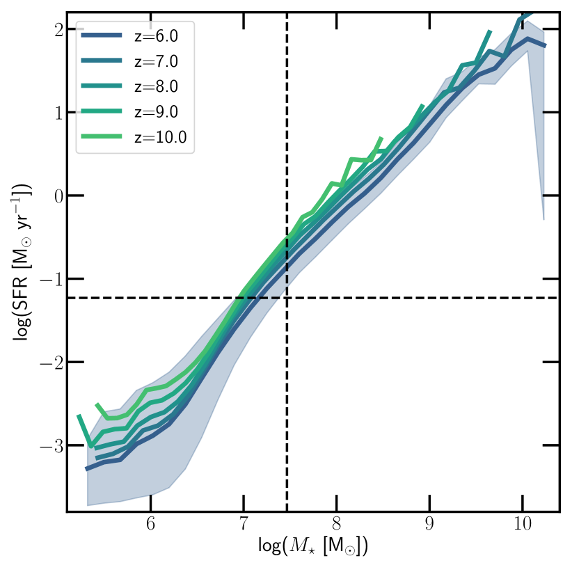
Figure 1: The star-formation rate as a function of the stellar mass of a galaxy at $z=6$–$10$ as indicated. The shaded region represents the $10^{\text{th}}$ and $90^{\text{th}}$ percentiles of the distribution at $z=6$. Similar scatter in the relation exists at other redshifts, which we have chosen not to show for the sake of clarity. For the skirt calculations, we only consider galaxies with stellar masses at least $50$ times larger than the baryonic mass resolution of the simulation (vertical line) and with at least one star particle less than $5$ Myr old (horizontal line).

Of particular relevance to this paper, the IllustrisTNG simulations have been post-processed using similar schemes to estimate the high-redshift luminosity functions, dust content (Vogelsberger et al., 2020b), dust attenuation curves and IR luminosity functions (Shen et al., 2020, 2022). We employ the same scheme as these works to estimate the emission line luminosities from the thesan simulations. Briefly, the intrinsic nebular emission is taken from Byler et al. (2017), which is based on photoionization calculations using cloudy. The underlying stellar radiation intensities and spectra are taken from the Flexible Stellar Population Synthesis (FSPS) model (Conroy et al., 2009). The calculations assume that the fraction of escaping Lyman continuum photons is zero and nebular emission is completely determined by the gas phase metallicity and the ionization parameter. The H ii regions are assumed to be dust free. Such an assumption is necessary in order to match the low mass end of the observed high-redshift UV luminosity functions (Vogelsberger et al., 2020b) and the equivalent widths (EWs) of the [O iii] +H $\beta$ aggregate emission line in high-$z$ galaxies (Shen et al., 2020). The gas phase metallicity of the H ii regions is chosen to be the same as the initial metallicity of the stellar particles, which is inherited from the gas cell from which a stellar particle is created. The ionization parameter, that encodes information about the intensity of the ionizing source and the geometry of the gas cloud is chosen to be $10^{-2}$ as suggested in Byler et al. (2018). Only young stellar populations (with ages less than 10 Myrs old) are assumed to be surrounded by their birth cloud and hence the nebular emission is only active for these stars. Older stars generally escape the birth clouds and, therefore, only contribute intrinsic radiation emission as given by the FSPS model (Shen et al., 2020). A slight inconsistency arises due to the fact that the nebular emission models are computed assuming a Kroupa (2001) model while the intrinsic stellar SEDs are calculated with a Chabrier (2003) IMF. However, this introduces only small differences in the computed galaxy SEDs and we are confident that the inconsistency in the population synthesis models does not have a significant impact on our results for all bands and all redshifts (see Vogelsberger et al., 2020b, for a more thorough discussion.).

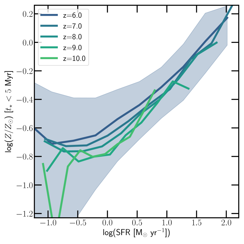
Figure 2: The star-formation rate–metallicity (in units of $Z_{\odot}$) relation for stars younger than $5$ Myr old at $z=6$–$10$ as indicated. The shaded region shows the $10^{\text{th}}$ and $90^{\text{th}}$ percentiles of the distribution at $z=6$. As the star-formation rate of the halo increases, the metallicity of newly formed stars increases considerably (by almost an order of magnitude). In contrast the redshift evolution is much less extreme.

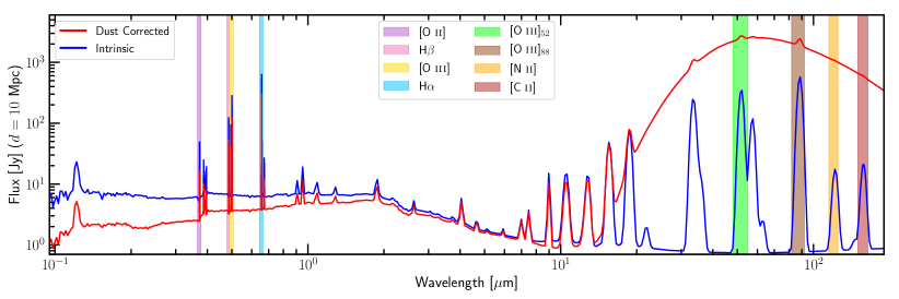
Figure 3: The rest frame spectral energy distribution of the central galaxy in the most massive halo in the thesan-1 simulation ($M_{\star}(<2r_{\mathrm{half},\star})\simeq 7\times 10^{9}\mathrm{M}_{\odot}$) at $z=6$. The blue curve shows the intrinsic emission and the red curve indicates the dust reprocessed SED. The different coloured vertical bands denote the positions of the various emission lines considered in this work. These are the four rest frame optical emission lines, [O ii] ($3726,3729$ Å), H $\beta$ ($4861$ Å), [O iii] ($4959,5007$ Å) and H $\alpha$ ($6563$ Å), and four fine structure emission lines in the IR, [O iii] ₅₂ ($52$ µm), [O iii] ₈₈ ($88$ µm), [N ii] ($122$ µm) and [C ii] ($158$ µm).

Dust attenuation is modelled using the Monte Carlo radiative transfer code skirt (Version 8; last described in Camps & Baes, 2020), which accurately captures scattering and absorption by dust throughout the entire wavelength range considered. The radiative transfer calculations are performed on a Voronoi grid constructed from positions of the gas cells in the galaxy, mirroring the structure and geometry of the arepo data as closely as possible. Although the thesan simulations include self-consistent dust modelling, they predict relatively low dust-to-metal ratios (DTM) in high metallicity environments. This leads to insufficient dust attenuation producing too many high luminosity galaxies (Kannan et al., 2022). We therefore use a spatially constant DTM that scales as $\mathrm{DTM}\simeq 0.9\times(z/2)^{-1.92}$, where $z$ is the redshift. This relation was primarily derived to match the observed evolution of the UV luminosity function in the IllustrisTNG simulations (Vogelsberger et al., 2020b). There is some evidence to suggest that the DTM ratios of high redshift galaxies are much lower than in the local Universe (see for example, Inoue, 2003; Aoyama et al., 2017; Behrens et al., 2019). However, recent observational evidences (De Cia et al., 2016; Wiseman et al., 2017) from damped Lyman-$\alpha$ absorbers do not show an obvious redshift dependence. In fact they show a much stronger correlation with the gas metallicity than redshift. Moreover, hydrodynamical simulations that include self-consistent dust modelling show that the DTM ratio can vary even within a single galaxy (Bekki, 2015; McKinnon et al., 2016). Estimating a more sophisticated DTM relation that depends on both metallicty and redshift is beyond the scope of this work. We therefore use the relation derived in Vogelsberger et al. (2020b) in this work and note that, in addition to the UV luminosity functions, this model has been relatively successful in estimating various emission line luminosities and IR luminosity functions as well (Shen et al., 2020, 2022).

Dust emission is modelled assuming thermal equilibrium with the local radiation field. A Draine & Li (2007) dust mixture of amorphous silicate and graphitic grains, including varying amounts of polycyclic aromatic hydrocarbons (PAHs) particles, is assumed. This model reproduces the average Milky Way extinction curve and is widely used (Jonsson et al., 2010; Rémy-Ruyer et al., 2014). Stars act as sources of radiation, with the smoothing length of the star particles used to calculate a smoothed photon source distribution function. For each wavelength on the wavelength grid, $N_{\mathrm{p}}$ photon packets are launched isotropically from the smoothed positions of the stellar particles. The photon packets then propagate through the resolved gas (dust) distribution in the ISM and interact with the dust cells randomly before they are finally collected by the photon detector, which is placed at a distance of 10 Mpc from the galaxy centre in the $+z$ direction. We set $N_{\mathrm{p}}$ equal to the number of all the stellar particles bound to a galaxy with an upper and lower bound of this value set to $10^{5}$ and $10^{2}$ respectively. The wavelength grid ranges from $0.05$ µm to $200$ µm, discretised into $657$ unequal bins, with increased resolution focused around the wavelengths of the emission lines considered in this work, which are the four rest frame optical emission lines, [O ii] ($3726,3729$ Å), H $\beta$ ($4861$ Å), [O iii] ($4959,5007$ Å) and H $\alpha$ ($6563$ Å), and four fine structure emission lines in the IR, [O iii] ₅₂ ($52$ µm), [O iii] ₈₈ ($88$ µm), [N ii] ($122$ µm) and [C ii] ($158$ µm).

Only sufficiently well-resolved, star-forming galaxies are considered, so as to ensure that the output SEDs from the skirt calculations are reasonably converged. We consider a galaxy well resolved if the stellar mass within twice the stellar half-mass radius is greater than $50$ times the baryonic mass resolution of the simulation. This limit is indicated by the vertical dashed line in Figure 1, which shows the star-formation rate of a galaxy as a function of its stellar mass in thesan-1 for $z=6$–$10$ as indicated. Most of the galaxies lie on the star-forming main sequence with similar slopes at all redshifts considered, although the amplitudes increase with redshift. Since most of the emission lines are related to the star-formation rate of the galaxy (Kennicutt, 1998), we also require that at least one star particle be less than $5$ Myrs old which ensures that there is recent on-going star formation within the halo. Given the resolution of the simulation, this roughly translates to haloes with a minimum star-formation rate of just below $0.1$ M_⊙ yr^-1 (dashed horizontal in Figure 1). For all selected haloes, we compute the SEDs and emission line luminosities arising from the central $30$ kpc of the galactic centre. The analysis is carried out for all haloes that match these criteria at $z=6$, $z=7$, $z=8$, $z=9$ and $z=10$. This translates to $\sim 10,000$ galaxies at $z=6$ and about $\sim 20,000$ in total.

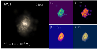
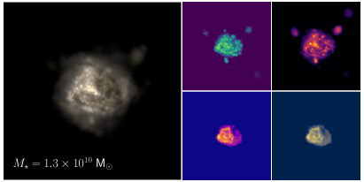
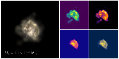
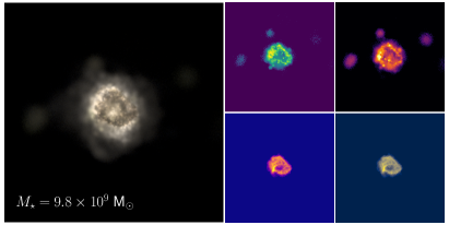
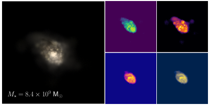
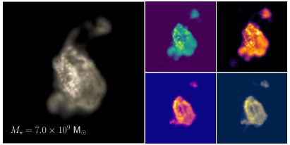
Figure 4: Face-on images of six massive galaxies in thesan-1 at $z=6$. The large panels on the left show mock JWST images constructed for the NIRCam F277W, F356W, and F444W filters. The smaller panels show resolved emission line maps (not continuum subtracted) of H $\alpha$, [O iii], [O iii]₈₈, and [C ii]. All images cover a $10\times 10$ kpc² field of view with $500\times 500$ pixels. The quoted stellar masses are within two times the stellar half-mass radius.

Figure 2 shows the mass-weighted metallicity (in units of the solar metallicity, $Z_{\odot}$) of all stars less than $5$ Myrs old as a function of the star-formation rate of the galaxy, for resolved, star-forming haloes as defined in the previous paragraph. The metallicities of these stars determine the strength of the metal nebular emission lines as they produce the largest amount of ionizing radiation (Conroy et al., 2009; Eldridge et al., 2017). The metallicity increases considerably, by almost an order of magnitude, with increasing star-formation rate. The evolution with redshift on the other hand is relatively gentle, with a difference of only about $0.2$ dex at a moderate SFR of $\sim 1\,\text{M}_{\odot}\,\text{yr}^{-1}$. Finally, Figure 3 shows both the intrinsic and dust-corrected SED of the central galaxy in the most massive halo in the thesan-1 simulation at $z=6$ ($M_{\star}(<2r_{\mathrm{half},\star})\simeq 7.01\times 10^{9}\mathrm{M}_{\odot}$). The different coloured vertical bands represent the various target emission lines considered in this work. We have chosen to investigate these particular lines because they are predicted to be some of the most luminous in high-$z$ galaxies and are planned to be observed by current and upcoming LIM experiments. Finally, we note that we have only performed this analysis on the thesan-1 simulation and any results presented in this work from other simulations in the thesan suite are derived on the assumption that the $L$–$\mathrm{SFR}$ scaling relations are converged between the resolutions (Kannan et al., 2022).

3 Results

3.1 Photometric properties

To illustrate the qualitative features of the radiative transfer calculations, we show in Figure 4 face-on images of six massive galaxies in thesan-1 at $z=6$. The large panels on the left show mock JWST images constructed for the NIRCam F277W, F356W, and F444W filters. The smaller panels show resolved emission line maps (not continuum subtracted) of select lines H $\alpha$, [O iii], [O iii]₈₈, and [C ii] as indicated. All images cover a $10\times 10$ kpc² field of view with $500\times 500$ pixels. The visualisations show the structural morphology of these massive galaxies, including the impact of dust and subtle differences in the emergent emission line maps.

A more quantitative analysis of the derived SED and emission line properties of the galaxies in thesan-1 begins with Figure 5, which shows the UV luminosity (at rest frame $1500$ Å) functions at $z=6$–$10$ as indicated. For comparison, we also show observational estimates (coloured points) from Bouwens et al. (2015); Bouwens et al. (2017), Finkelstein et al. (2015), McLeod et al. (2016), Livermore et al. (2017), Atek et al. (2018) and Ishigaki et al. (2018). The dashed curves show the intrinsic luminosities of the galaxies, while the solid curves display the dust-attenuated luminosity functions, with the shaded regions indicating the Poisson noise. The simulated luminosity functions start to fall off at $M_{\mathrm{UV}}\gtrsim-18$, because we chose to model only galaxies above a certain stellar mass and SFR. Kannan et al. (2022) shows that the luminosity functions continue with the same slope up to $M_{\mathrm{UV}}\simeq-12$ in the thesan-1 simulation when all the galaxies in the simulation volume are considered. Dust attenuation manages to reduce the UV magnitudes of the most massive star-forming galaxies ($M_{\mathrm{UV}}\lesssim-21$), such that the simulated estimates match the observational results at almost all redshifts ($z\geq 7$). At $z=6$ however, the model seems to slightly under-predict the dust attenuation at the high mass end, indicating that the DTM ratios might need to be even higher than what is predicted from the scaling relation used in this work. Overall, this figure confirms that our SED modelling give rise to realistic UV luminosities. Moreover, the dust attenuation model does a reasonable job of reducing the UV luminosites of highly star-forming galaxies, such that the simulated UVLF reproduces the observed drop-off at the right magnitudes and by roughly the correct amount.

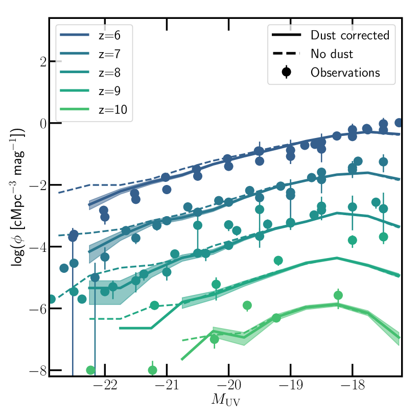
Figure 5: UV luminosity (at rest frame $1500$ Å) functions at $z=6$–$10$, for thesan-1 derived from the skirt calculations. The dashed curves show the intrinsic emission of the galaxy while the solid curves are the dust-attenuated values. The observational estimates are taken from Bouwens et al. (2015); Bouwens et al. (2017), Finkelstein et al. (2015), McLeod et al. (2016), Livermore et al. (2017), Ishigaki et al. (2018) and Atek et al. (2018). We note that the luminosity functions are offset by $\Delta\mathrm{log}(\Phi)=-(z-8)$. The simulated UV luminosity functions match the observational estimates over a wide range of magnitudes.

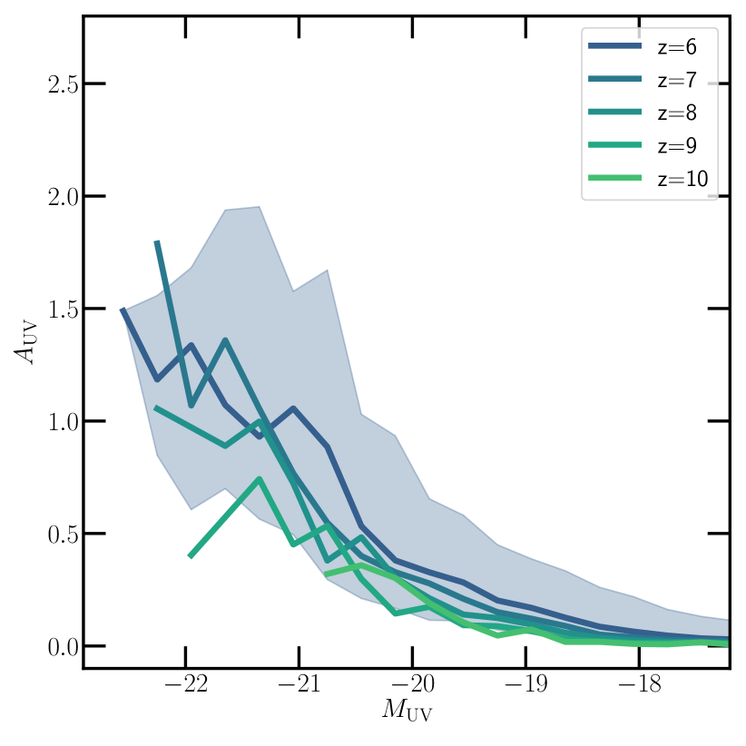
Figure 6: The attenuation, $\mathrm{A_{UV}=-2.5~{}log(L_{UV}^{observed}/L_{UV}^{intrinsic})}$, at UV wavelengths as a function of the UV magnitude for the galaxies in thesan-1 at $z=6$–$10$ as indicated. The shaded regions shows the $10$–$90$ percentile distribution at $z=6$. While the low luminosity galaxies are largely dust free, the high mass, high SFR, metal enriched galaxies show a steep increase in dust attenuation, especially below $M_{\mathrm{UV}}\lesssim-21$. This sharp rise in $A_{\mathrm{UV}}$ is needed in order to match the steep fall off in the observed UVLF happening at about the same magnitude.

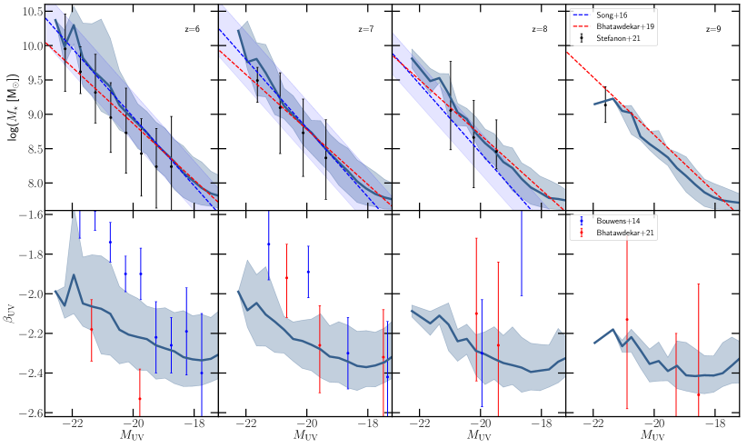
Figure 7: Top panels: The stellar mass of the galaxies as a function of the dust-corrected UV magnitude at $z=6$ (first panel), $z=7$ (second panel), $z=8$ (third panel) and $z=9$ (fourth panel). For comparison, we also show observational estimates from Song et al. (2016, blue curves), Bhatawdekar et al. (2019, red curves), and Stefanon et al. (2021, black points). Bottom panels: The UV continuum slope ($1300$–$2650$ Å) as a function of the UV magnitude of the galaxies for $z=6$–$9$ as indicated. The shaded regions show the $2\sigma$ scatter in the relation. Observational estimates from Bouwens et al. (2014) and Bhatawdekar & Conselice (2021) are shown as blue and red points, respectively.

The impact of dust is seen more clearly in Figure 6, which plots the attenuation of the UV flux, $A_{\mathrm{UV}}=-2.5~{}\mathrm{log}(L_{\mathrm{UV}}^{\mathrm{observed}}/L_{\mathrm{UV}}^{\mathrm{intrinsic}})$, as a function of the dust-attenuated UV magnitude of the galaxies at $z=6$–$10$. As expected, the low luminosity ($M_{\mathrm{UV}}\gtrsim-19$) and by extension low SFR galaxies are least affected by dust. In fact $A_{\mathrm{UV}}\sim 0$, for these low mass haloes, implying that they are effectively dust free. This is because the low SFR haloes are less metal enriched (Figure 2), therefore the dust content and corresponding attenuation is lower. As the SFR increases, the galaxies become more metal enriched and dust obscured. Additionally, the slight evolution in the metallicity and DTM ratio with redshift imprints a corresponding evolution in the attenuation factor. At higher redshifts, galaxies have $A_{\mathrm{UV}}\sim 0.5$ even at $M_{\mathrm{UV}}\lesssim-21$. On the other hand the attenuation is much more rapid at $z=6$ with an almost exponential increase in the UV attenuation for galaxies brighter than $M_{\mathrm{UV}}\lesssim-20$, hinting at a rapid buildup of dusty, high-mass, high-SFR galaxies during the reionization epoch. This steep increase in $A_{\mathrm{UV}}$ is needed to account for the steep drop-off in the observed UVLF happening at about the same magnitude. The shaded region shows the scatter in this relation, which is quite large especially for the highest luminosity galaxies. The scatter mainly arises because the viewing angle of the galaxy is random. For example, a galaxy viewed edge-on will have significantly more attenuation than one that is face-on. The impact of viewing angle on the attenuation curve of galaxies will be investigated in future works.

In the top panels of Figure 7 we show the stellar mass of the galaxies as a function of the dust-corrected UV magnitude at $z=6$–$9$ as indicated. The solid curves show the median and the shaded regions represent the $2\sigma$ scatter around it. The dashed blue curves and black points show the observational data derived using stellar mass estimates from deep IRAC/Spitzer measurements of galaxies in the reionization epoch as outlined in Song et al. (2016) and Stefanon et al. (2021), respectively. The dashed red lines are the best-fit curves to the stellar masses derived for the galaxies in the Hubble Frontier Fields by combining the HST imaging with Spitzer and ground-based VLT data (Bhatawdekar et al., 2019). At lower redshifts ($z=6$ and $z=7$), the simulations seems to be in better agreement with the Song et al. (2016) data, while Bhatawdekar et al. (2019) and Stefanon et al. (2021) match the simulated values for $z=8$ and $z=9$ more accurately. The scatter in the relation from the simulations is consistent with the observational scatter.

Along similar lines, the bottom panels of Figure 7 present the UV continuum slopes ($\beta_{\mathrm{UV}}$) as a function of the galaxy UV magnitude at $z=6$ (first panel), $z=7$ (second panel), $z=8$ (third panel) and $z=9$ (fourth panel). The UV continuum depends on the mass and surface temperature of the O & B stars, therefore, it will change according to the underlying IMF and the metal enrichment within the galaxies. Moreover, the star formation history of a galaxy will determine the number of young stars and, hence, the UV slopes also contain information about the recent star formation episodes within the galaxies. Finally, the UV continuum is also affected by the distribution of dust and their grain size distribution (see for example Reddy et al., 2012). Therefore, this measurement helps constrain a variety of physical properties that govern galaxy formation (Wilkins et al., 2013). The slopes are measured by fitting the dust-attenuated SEDs in the $10$ wavelength filters suggested by Calzetti et al. (1994), with a power-law function, $f_{\lambda}\propto\lambda^{\beta_{\mathrm{UV}}}$. The shaded regions show the $2\sigma$ scatter around the median. The red and blue points show observational estimates from Bouwens et al. (2014) and Bhatawdekar & Conselice (2021), respectively. At $z=6$, the two observational works are in tension with the Bouwens et al. (2014) estimates, showing consistently higher values than the results from Bhatawdekar & Conselice (2021). At higher redshifts, the estimates are more compatible with each other. The simulated low luminosity galaxies ($M_{\mathrm{UV}}\gtrsim-19$) match the Bouwens et al. (2014) values at $z=6$ and lie above the estimates from Bhatawdekar & Conselice (2021). At higher redshifts they are in general agreement with both the observational estimates. Since most of these galaxies are mainly dust free, these results imply that the underlying IMF and SFRs of the simulated galaxies are in general agreement with the observationally inferred estimates. The observed UV continuum slopes of massive galaxies diverge, with Bouwens et al. (2014) showing a steep increase in $\beta_{\mathrm{UV}}$, while Bhatawdekar & Conselice (2021) predict a relatively redshift independent evolution. However, we caution that the Bhatawdekar & Conselice (2021) data predicts that bright galaxies at $z=6$ are significantly bluer than the bright galaxies at $z=7$, which is contrary to the general picture of galaxies getting more dust enriched with time. Therefore, the bright galaxies in the thesan simulations seem to show shallow UV continuum slopes that are in tension with the observed data. This might be a consequence of the assumed DTM scaling, which evolves very strongly with redshift, leading to too little dust at these high redshifts. Similar discrepancies have been found in other simulation efforts (Gnedin, 2014; Shen et al., 2020; Wu et al., 2020; Vijayan et al., 2021) and they may be attributed to disparate extinction curves at high-$z$. An investigation into the variations caused by different extinction curves is beyond the scope of this paper, but we refer the reader to Shen et al. (2020) for a more extensive discussion of this topic. These three plots (Figures 5, 6 and 7) indicate that the simulations and SED model do a good job of reproducing the observed UV properties and magnitude of dust attenuation in high-redshift galaxies.

Figure 8: The emission line luminosities of [O ii] (first panel), H $\beta$ (second panel), [O iii] (third panel), H $\alpha$ (fourth panel), [O iii]₅₂ (fifth panel), [O iii]₈₈ (sixth pnael), [N ii] (seventh panel) and [C ii] (eighth panel) as a function of the SFR of the galaxies at $z=6$–$10$ as indicated. The shaded regions show the $10^{\text{th}}$ and $90^{\text{th}}$ percentiles of the distribution at $z=6$. The dashed black curves show the best-fit relation using Eq. (1). Observational and theoretical estimates from Kennicutt (1998, dashed red curves), Ly et al. (2007, dashed blue curves), De Looze et al. (2014, dashed magenta curves), Lagache et al. (2018, dashed cyan curves), Rigopoulou et al. (2018, dashed brown curves) and Leung et al. (2020, dashed yellow curves) are also shown for comparison. In general, the predicted emission line luminosities are in good agreement with the estimates found in the literature, although important differences exist.

3.2 Emission line luminosities

We now shift our focus to measuring the luminosities of the emission lines considered in this work. In Figure 8 we plot the line luminosities (in L_⊙) of [O ii] (first panel), H $\beta$ (second panel), [O iii] (third panel), H $\alpha$ (fourth panel), [O iii]₅₂ (fifth panel) [O iii]₈₈ (sixth panel) [N ii] (seventh panel) and [C ii] (eighth panel) as a function of the SFR of the galaxies. The solid lines indicate the median relation from the simulation, with the various colours denoting the different redshifts from $z=6$–$10$ as indicated. The corresponding shaded regions show the $10^{\text{th}}$ and $90^{\text{th}}$ percentiles of the distribution at $z=6$. Similar scatter is observed at higher redshifts as well, but this is not shown in order to maintain the clarity of the plot. The median relation shows minimal evolution with redshift for all the lines considered in this work, because of the sluggish evolution in the metallicity of H ii regions with redshift (see Figure 2). In fact, the median relations at all redshifts more or less lie on top of each other, with the relative spread much smaller than the scatter in the relations at $z=6$.

We therefore choose to quantify the line luminosities as a function of the SFR alone using a broken power-law fit of the form

$$y=\left\{\begin{array}[]{ll}a+m_{a}x&x<x_{b}\\ a+(m_{a}-m_{b})x_{b}+m_{b}x&x_{b}\leq x<x_{c}\\ a+(m_{a}-m_{b})x_{b}+(m_{b}-m_{c})x_{c}+m_{c}x&\text{otherwise}\end{array}\right.$$ (1)

where $y=\mathrm{log}(L\,/\,\mathrm{L}_{\odot})$ and $x=\mathrm{log(SFR)}$ in units of $\mathrm{M_{\odot}\,yr^{-1}}$. The fit involves three regimes. First, $x<x_{b}$, which encapsulates the behaviour at low star-formation rates corresponding to line emission from low metallicity dust-free galaxies. The intermediate regime ($x_{b}\lesssim x<x_{c}$) accounts for the slightly metal and dust enriched galaxies with relatively low dust attenuation. Finally, at high star-formation rates, the galaxies are highly metal enriched, which in turn leads to high dust masses and high levels of attenuation. As the low star-formation rate galaxies (SFR$\lesssim 1$ M_⊙ yr^-1) are largely dust free, we set $x_{b}=0$, while all the other parameters are fit using the method of least squares. Additionally, the far-IR lines are not expected to be attenuated by dust (Draine & Li, 2007), so we only use a single power law for these lines. The best-fit values for the different lines and their $1\sigma$ error are summarised in Table 2.

Table 2: Best-fit values and $1\sigma$ error bars for the emission line luminosity as a function of the star-formation rate of the galaxy. The table lists the names (first column) and wavelengths (second column) of the lines considered in this work along with the parameters used to describe the $L$–$\mathrm{SFR}$ relation (columns three to seven) as outlined in Eq. (1).

Line	Wavelength (Å)	$a$	$m_{a}$	$m_{b}$	$m_{c}$	$x_{c}$
[O ii]	3726, 3729	7.08 $\pm$ 0.006	1.11 $\pm$ 0.016	1.31 $\pm$ 0.030	0.64 $\pm$ 0.031	0.54 $\pm$ 0.032
H $\beta$	4861	7.62 $\pm$ 0.002	0.96 $\pm$ 0.007	0.86 $\pm$ 0.008	0.41 $\pm$ 0.027	0.96 $\pm$ 0.035
[O iii]	4959, 5007	7.84 $\pm$ 0.006	1.24 $\pm$ 0.016	1.19 $\pm$ 0.027	0.53 $\pm$ 0.039	0.66 $\pm$ 0.040
H $\alpha$	6563	8.08 $\pm$ 0.002	0.96 $\pm$ 0.006	0.88 $\pm$ 0.008	0.45 $\pm$ 0.025	0.96 $\pm$ 0.032
[O iii]52	$5.2\times 10^{5}$	6.75 $\pm$ 0.007	1.47 $\pm$ 0.013	-	-	-
[O iii]88	$8.8\times 10^{5}$	6.98 $\pm$ 0.008	1.37 $\pm$ 0.014	-	-	-
[N ii]	$1.22\times 10^{6}$	4.42 $\pm$ 0.010	1.83 $\pm$ 0.018	-	-	-
[C ii]	$1.58\times 10^{6}$	5.01 $\pm$ 0.005	1.49 $\pm$ 0.011	-	-	-

The ionized hydrogen gas in H ii regions recombines in a cascading process that produces various strong emission lines including H $\alpha$ and H $\beta$. The line luminosities show an almost linear relation with SFR at low SFRs. It then becomes shallower due to increased dust attenuation. Encouragingly, the intrinsic H $\alpha$/H $\beta$ ratio is about $2.9$ which is very close the theoretical value of $2.87$ that assumes an electron temperature of $T_{e}=10^{4}~{}\mathrm{K}$, an electron density of $n_{\rm e}=10^{2}~{}\mathrm{cm}^{-3}$, and Case B recombination conditions (Osterbrock & Ferland, 2006). The dashed red curves show the estimates from Kennicutt (1998), who assumed an optically thick ISM, case B recombination, a Salpeter (1955) IMF and that all UV continuum is absorbed by the gas in the galaxy. The plotted relation has been re-scaled to match a Kroupa (2001) IMF adopted in this work by using the conversion presented in Driver et al. (2013). The intrinsic luminosities of these Balmer lines (devoid of any dust attenuation) derived from the thesan simulations is about a factor of $0.3$ dex higher and the slopes are slightly shallower than the values obtained by Kennicutt (1998). These differences arise due to the fact that the low SFR galaxies also have low stellar metallicities, leading to an increased output of ionizing photons, resulting in a higher H $\alpha$ and H $\beta$ luminosity. In fact, it has been shown that decreasing the metallicity can increase the Balmer line luminosities by about $\sim 0.25$ dex (Leja et al., 2017). This will increase the luminosity of the Balmer emission lines at low SFR while maintaining similar values in galaxies which contain stars that have $Z_{\star}\sim Z_{\odot}$, which in our simulations happens only in the rare highly star-forming haloes (Figure 2). This effect, therefore, explains the discrepancies seen in both the amplitude and slope of the relation.

Ionized oxygen in the H ii regions produces a variety of emission lines in both the optical and FIR. We first look at the forbidden [O ii] ($3726,3729$ Å) doublet. Similar to the Balmer lines, we show the rescaled estimate from Kennicutt (1998, dashed red curve). The simulated values are slightly below the expected relation due to the low metallicity of H ii regions in low SFR galaxies. The luminosities increase with a power law slope greater than one, as the metallicity increases with the SFR. At high SFRs dust attenuation kicks in and reduces the expected luminosities again. Another important oxygen emission line in the visible spectrum is the [O iii] ($4959,5007$ Å) doublet. For comparison we show the observational estimates from Ly et al. (2007, dashed blue curve), who derived the relation from $197$ galaxies in the redshift range $0.07$–$1.47$ from the Subaru Deep Field. Akin to the [O ii] scaling relation, the line luminosities at low SFR are lower than the expected values due to the low metallicity of H ii regions and then increase with a super-linear power law slope until dust attenuation becomes significant and reduces the luminosities again.

The far-infrared (FIR) fine-structure lines of carbon, nitrogen and oxygen are among the most dominant coolants in the ISM of galaxies. They are excellent extinction-free probes of the physical conditions of the gas and the intensity and hardness of the ambient interstellar radiation fields (Ferkinhoff et al., 2010). We start with the [O iii] lines at $52$ µm and $88$ µm (bottom left panels of Fig. 8). Since the ionization potential for doubly ionized oxygen is $35$ eV, the O iii regions reside close to the hot and young O stars. This makes the [O iii] emission co-spatial with the other strong nebular emission lines like the Balmer lines making them important tracers of the star formation in the galaxy. Overplotted is the observed relation for [O iii]₈₈ from De Looze et al. (2014) who derived the relation using a sample of low-metallicity dwarf galaxies from the Herschel Dwarf Galaxy Survey and a broad sample of galaxies of various types and metallicities from the literature. The simulated relation appears to be slightly steeper than the observed one, however, they do match over a wide range in SFR ($0<\mathrm{SFR[M_{\odot}\,yr^{-1}]}<2$) within the errorbars, but disagree at very low metallicities/SFRs by about $0.3$ dex. The luminosity of the [O iii]₅₂ line is similar to that of [O iii]₈₈, mainly because the line ratio is about $\sim 1$ in most environments and is completely insensitive to the metallicity of the H ii region and is only slightly dependent on the density of the ionized cloud (Yang et al., 2021).

Another important nebular emission line is the fine structure line of the singly ionized nitrogen atom, [N ii] at rest frame $122$ µm. Photons of energy greater than $14.5$ eV are needed to ionize the neutral N atom, implying that the [N ii] line emission mainly arises in highly photoionized H ii regions around old O and young B stars (Ferkinhoff et al., 2011). The simulated median relation (third panel from the left in the bottom row of Figure 8) shows a very steep power law slope of around $\sim 1.8$, which is in disagreement with observations from Spinoglio et al. (2012) who estimate a power law slope of $\sim 1$. However, these observations were made at low redshifts and do not fully account for the low metallicities of high-redshift galaxies. It has recently been shown that the [N ii] luminosity falls off rapidly with decreasing metallicity and can therefore be used as a metallicity indicator for high-redshift galaxies (Rigopoulou et al., 2018). We therefore estimate the expected $L_{[\text{N\,{ii}}]}$–SFR relation by combining the $L_{[\text{O\,{iii}}]_{88}}$–SFR relation of De Looze et al. (2014) with the metallicity dependant [O iii]₈₈/ [N ii] line ratio derived in Rigopoulou et al. (2018). We specifically consider models with the ionization parameter $U_{\mathrm{ion}}=10^{-2}$, which matches the parameters used in this work. The metallicity at a particular SFR is taken self-consistently from the simulations as shown in Figure 2. The resulting relation is shown as a brown curve in the panel. The simulated values and the derived relation lie on top of each other, thereby highlighting the importance of understanding line emission luminosities in low metallicity environments in order to make accurate predictions for line intensity mapping studies that target the Epoch of Reionization.

Finally, we turn our attention to luminosities for the $158$ µm line emitted by the singly ionized C⁺ atom. The relatively low ionization potential of carbon ($\sim 11.2$ eV) makes C⁺ one of the most abundant metal ions in a variety of environments. Its fine structure line, [C ii], provides the most efficient cooling mechanism for gas in PDRs. This line is also emitted from ionized regions, cold atomic gas and CO dark clouds (Olsen et al., 2015). It is therefore often the strongest IR emission line in galaxy spectra. Moreover, this line is easily accessible from the ground at $4.5\lesssim z\lesssim 8.5$. The extensive abundance of [C ii] emission line environments makes predicting the line luminosities extremely difficult. An accurate estimate will require robust H ii region modelling coupled with self-consistent temperature and radiation field intensities in the PDRs. These in turn will depend on the metal and dust distributions within galaxies. Therefore fully-coupled RHD simulations, that resolve the multi-phase structure of the ISM (Pallottini et al., 2019; Katz et al., 2019; Lupi et al., 2020) are required to properly model [C ii] line luminosities. However, these simulations are computationally expensive restricting our ability to make simultaneous predictions in a variety of environments.

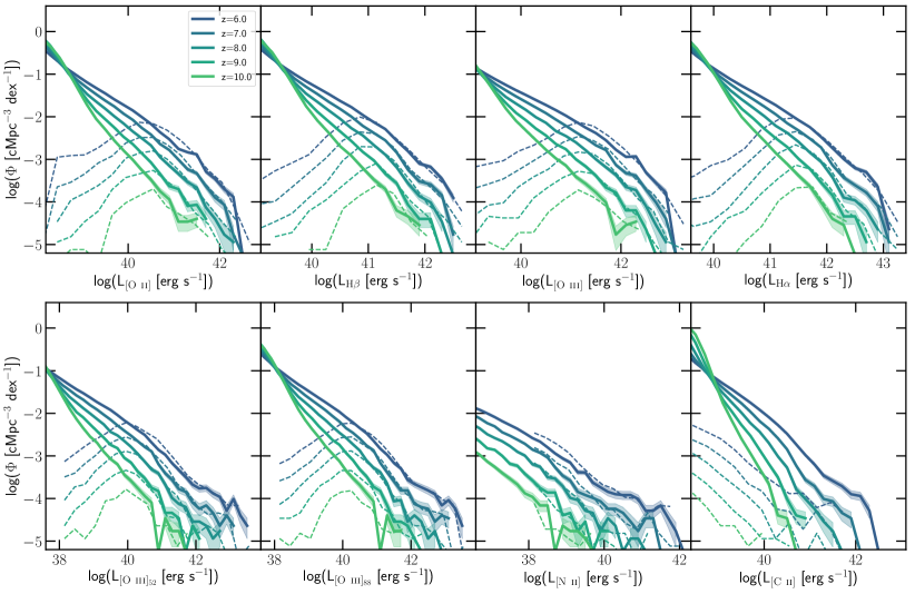
Figure 9: The line luminosity functions of the eight emission lines considered in this work at $z=6-10$ as indicated. The dashed curves show the luminosity functions derived using the values obtained by the SED modelling technique described in Section 2. The decline at low luminosities arises from the selection function that only includes emission from haloes that are ‘resolved’ ($M_{\star}\gtrsim 3\times 10^{7}$ M_⊙) and have relatively high star-formation rates ($\gtrsim 0.1$ M_⊙ yr^-1). The solid curves, on the other hand, are luminosity functions estimated from the best-fit relations (outlined in Table 2) applied to all identified subhaloes in the simulation with a non-zero star-formation rate.

Recent theoretical efforts have focused on using sub-resolution H ii region and PDR modelling of the galaxies in semi-analytic models (Lagache et al., 2018, dashed cyan curve) and hydrodynamic simulations (Leung et al., 2020, dashed yellow curves) to predict [C ii] emission line luminosities in a wide variety of environments. Our estimates fall below the luminosity predictions from earlier works, especially in low SFR galaxies, most likely because we are unable to properly model the PDR and CO dark molecular regions. This will require a realistic model for the far-UV radiation field intensity in the galaxy and correct gas temperatures in the PDR regions, which depends on the photoelectric heating rate, which in turn will depend on the dust content. We plan to improve our estimates in a future work using RHD simulations that self-consistently model the dust content, molecular gas and radiation field intensities in galaxies (Kannan et al., 2020; Kannan et al., 2021). In particular, this will be part of the thesan-zooms simulation suite that simulates galaxies with a wide range of halo masses ($10^{8}$–$10^{12}\,\mathrm{M}_{\odot}$). For the current work, however, we assume that the [C ii]–SFR relation given by Lagache et al. (2018) is sufficiently accurate and proceed with further analysis.

Finally, in Figure 9 we show the line luminosity functions of the eight emission lines considered in this work at $z=6$–$10$ as indicated. For comparison, the dashed curves show the luminosity functions derived using the values obtained by the SED modelling technique described in Section 2. The decline at low luminosities arises from the incomplete selection function that only models emission from haloes that are ‘well-resolved’ ($M_{\star}\gtrsim 3\times 10^{7}$ M_⊙) and have relatively high star-formation rates ($\gtrsim 0.1$ M_⊙ yr^-1). The solid curves, on the other hand, are luminosity functions estimated from the best-fit relations (outlined in Table 2) applied to all identified subhaloes in the simulation with a positive star-formation rate. The star-formation rate of a galaxy is calculated by summing up all the SF probabilities of the cells in the equation of state (see Springel & Hernquist, 2003, for more details). This allows us to get an accurate estimate of the current star-formation rate of a galaxy and gets rid of the inherent noise arising from the probabilistic nature of the star formation and star particle creation routine. The fitting functions do a good job of reproducing the luminosity function at the high luminosity end where the selection function is complete. More importantly they are able to make predictions for luminosities of the various emission lines down to the resolution limit of the simulation. This is especially important for making LIM predictions as they are generally sensitive to all sources of emission, including low-mass galaxies. We note that the extrapolated luminosity functions of [C ii] do not match the predicted ones from SED modelling because we choose to show luminosity functions using the relation from Lagache et al. (2018), instead of the derived fits from our model, which we know to be inaccurate.

3.3 Line intensity maps and auto-correlation spectra

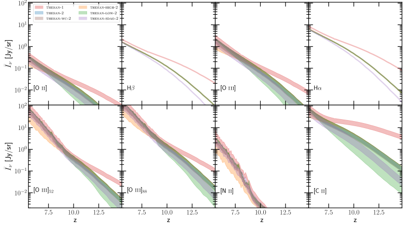
Figure 10: Mean intensity (defined in Eq. 2) of the eight emission lines considered in this work, as a function of redshift. The different coloured lines shows the estimates for thesan-1 (red curves), thesan-2 (blue curves), thesan-wc-2 (brown curves), thesan-high-2 (orange curves), thesan-low-2 (green curves) and thesan-sdao-2 (purple curves). The shaded regions indicate the uncertainty in the intensity arising from the unknown fraction of LyC photons escaping from nascent H ii regions. The mean intensity of all the lines increases towards lower redshifts mirroring the increase in the global star-formation rate density.

The fitting functions derived in the previous section allow us to generate emission line maps based solely upon the position, peculiar velocity (to account for redshift space distortions; Mao et al., 2012; Qin et al., 2022) and star-formation rate of the galaxy in the simulated volume. We start with Figure 10, which shows the average observed signal or mean intensity ($\bar{I}_{\nu}$) of the various emission lines as a function of redshift. Specifically, $\bar{I}_{\nu}$ is defined as (Fonseca et al., 2017)

$$\bar{I}_{\nu}=\frac{c}{4\pi}\frac{1}{\nu H(z)}\frac{\sum L_{\nu}(\mathrm{SFR})}{V_{\mathrm{box}}}\,,$$ (2)

where $c$ is the speed of light, $\nu$ is the frequency of the emission line in the rest frame of the galaxy, $H(z)$ is the Hubble constant at redshift $z$, $L_{\nu}$ is the luminosity of the emission line and $V_{\mathrm{box}}$ is the comoving volume of the simulation box. The different colours correspond to the different simulations in the thesan suite, with the red, blue, brown, orange, green and purple curves showing results from thesan-1, thesan-2, thesan-wc-2, thesan-high-2, thesan-low-2 and thesan-sdao-2 simulations, respectively.

The shaded regions represent the uncertainty in the mean intensity arising from the unknown fraction of LyC photons that escape the H ii regions. While, the emission line analysis assumes that the escape fraction is zero, we know that this cannot be true because such an assumption would not reionize the Universe. In the thesan simulations, an escape fraction ($f_{\mathrm{esc}}$) is applied to LyC photons to mimic these processes occurring below the grid scale of the simulation. Multiplying the emission line luminosity of the galaxy with $1-f_{\mathrm{esc}}$ gives us a lower limit on the amount of emission from these galaxies, while assuming all the LyC emission is absorbed and converted to emission lines from ionized gas sets an upper limit. The mean intensity of the hydrogen emission lines is unaffected by the escape of LyC photons because these photons will eventually interact with a neutral hydrogen atom in the Universe, ionizing it. So the total mean intensity will remain the same but it will alter the spatial distribution of the emission lines, which in turn will imprint a change in the power spectrum.

Figure 11: The 21 cm emission maps (first row) in thesan-1 at $z=9$ (first column), $z=8$ (second column), $z=7$ (third column) and $z=6$ (fourth column) compared to the surface brightness maps of the strong nebular emission lines like H $\alpha$ (second row), [O iii] (third row), [O iii] ₈₈ (fourth row) and [C ii] (fifth row). The 21 cm emission starts off quite uniform and gradually diminishes in the ionized regions as reionization progresses. Most of the nebular emission lines are concentrated in the high density filaments which host the star-forming galaxies. H $\alpha$ has an additional diffuse component that arises from the radiative recombination of ionized hydrogen throughout the Universe.

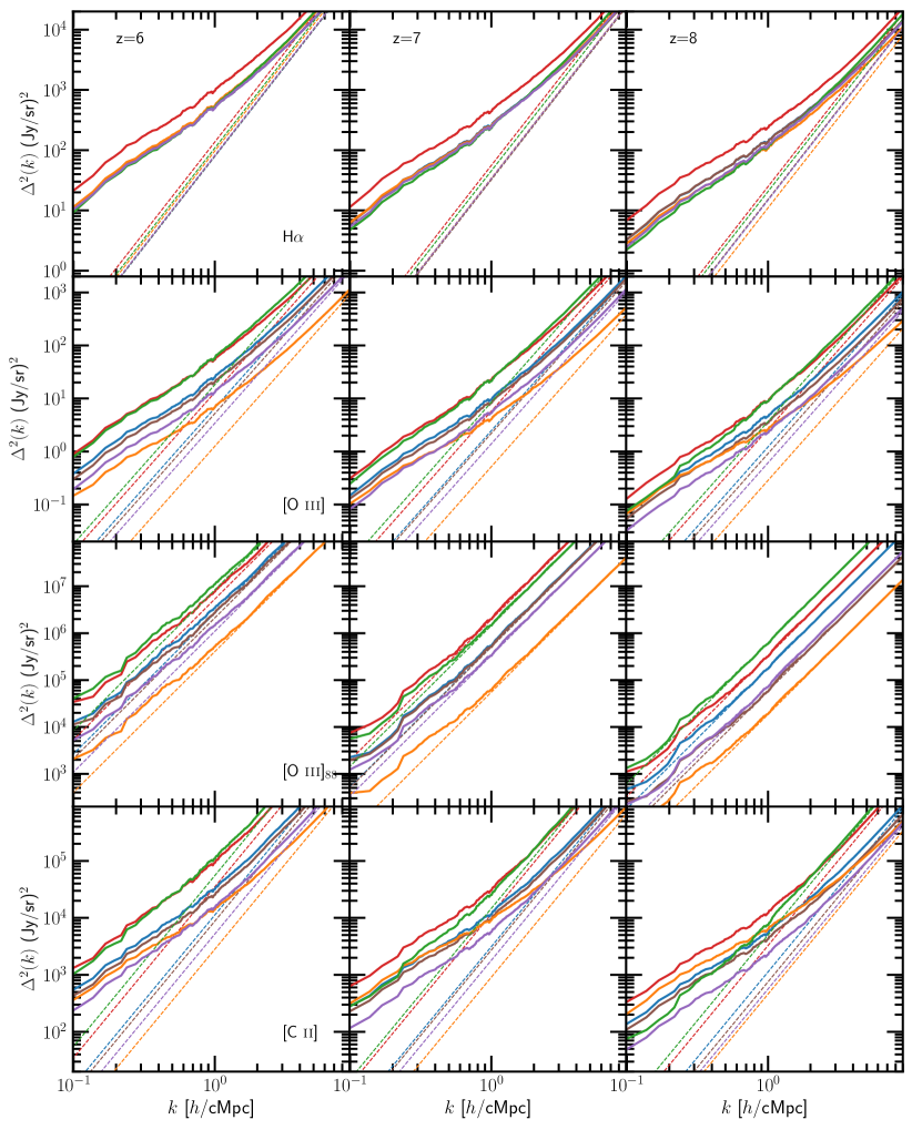
Figure 12: The power spectra of the H $\alpha$ (first row), [O iii] (second row), [O iii] ₈₈ (third row) and [C ii] (fourth row) emission lines at $z=6-8$, as indicated. The solid lines show the power spectrum while the dashed curves indicate the shotnoise contribution to it. The different coloured lines indicate the different simulations in our suite, namely, thesan-1 (red curves), thesan-2 (blue curves), thesan-wc-2 (brown curves), thesan-high-2 (orange curves), thesan-low-2 (green curves) and thesan-sdao-2 (purple curves).

We note that, while the $L$–$\mathrm{SFR}$ relation has been derived from emission line modelling of thesan-1 galaxies, we make the assumption that the relation holds true for the other simulations in our suite as well and calculate the intensity based on just the SFR of the galaxies. This assumption is valid because the resolved galaxy properties are relatively well converged with respect to resolution (Kannan et al., 2022). The mean intensity rises with decreasing redshift mirroring the increase in the global star-formation rate density (Madau & Dickinson, 2014). The predicted intensity of the lines at $z\lesssim 8$ is similar in all the simulations modulo the differences in the escape fractions. At higher redshifts, however, thesan-1 predicts significantly stronger emission line intensities because of the increased star-formation rate in low mass haloes. The mean intensities of the metal emission lines show a steeper evolution with redshift than the Balmer lines, because of the additional dependence on the metallicity that decreases with the SFR of the galaxy. We note that the estimated mean intensities of the [O ii] and [O iii] lines are roughly consistent (within a factor of $2$) with the Gong et al. (2017) estimate if extrapolated beyond $z\sim 5$. The Balmer emission lines, however, are a factor of $\sim 3-4$ higher, due to the increased emission from low metallicity galaxies and the slightly higher star formation rate density. It is quite clear that even measurements of this zeroth order quantity in conjunction with the global star-formation rate density will provide important insights into the $L$–$\mathrm{SFR}$ relation at these redshifts which will in turn place important constraints on the metal content and LyC production rate of these early galaxies.

In Figure 11 we show the spatial distribution of the 21 cm emission (first row) compared to the surface brightness maps of the four brightest lines considered in this work, namely, H $\alpha$ (second row), [O iii] (third row), [O iii] ₈₈ (fourth row) and [C ii] (fifth row) at $z=6$–$9$ as indicated in the thesan-1 simulation. The 21 cm emission is fairly uniform in the beginning, because almost all the gas in the Universe is neutral. At these redshifts the fluctuations in the 21 cm emission arise from the underlying fluctuations in the matter density field. As reionization progresses, the fluctuations increase as the ionized regions become dark. Eventually, all the gas in the Universe stops emitting in 21 cm, except for the gas in the high density filaments and galaxies that are self-shielded against the background radiation field. The substructures are quite important because they contribute almost $50\%$ to the 21 cm power spectrum at scales $k\sim 0.1$–$1$ $h$/cMpc (Kaurov & Gnedin, 2016). These scales are expected to be the most foreground-free in observations (DeBoer et al., 2017). It is therefore important for reionization simulations to resolve these features in order to accurately predict the 21 cm power spectrum (PS), especially during the end stages of the reionization process. Simulations that achieve a very low resolution for the radiative transfer calculations in the IGM ($\sim 200$–$330$ ckpc; Iliev et al. 2014; Hassan et al. 2021; Heneka & Cooray 2021) will not be able to properly resolve these filamentary structures, and will therefore yield inaccurate auto- and cross-correlation power spectra of the 21 cm line.

In the second row of panels in Figure 11 we show the H $\alpha$ emission, both from galaxies and diffuse emission from the recombination of the ionized hydrogen in the IGM. The H $\alpha$ radiative recombination luminosity in these resolved emission regions is given by

$$L_{\text{H\,{$\alpha$}}}^{\mathrm{rec}}=h\nu_{\text{H\,{$\alpha$}}}\int P_{\mathrm{B}}\,\alpha_{\mathrm{B}}(T)\,n_{e}\,n_{p}~{}\mathrm{d}V~{},$$ (3)

where $h\nu_{\text{H\,{$\alpha$}}}=1.89$ eV, $P_{\mathrm{B}}$ is the conversion probability per recombination event, which for H $\alpha$ is approximately $0.45$ (Storey & Hummer, 1995), $\alpha_{\mathrm{B}}$ is the case B recombination rate, $n_{e}$ and $n_{p}$ are the number densities of electrons and protons respectively, and $\mathrm{d}V$ is the volume of the cell. We calculate this quantity only for the diffuse gas in the simulation which is not on the equation of state (Springel & Hernquist, 2003). We note that the diffuse emission contributes only about $10$–$15\%$ of the total emission in the simulated volume. The major contribution is from ionized H ii regions around newly formed stars in galaxies. The maps clearly show that the most luminous regions of H $\alpha$ emission are centred around high density filaments and knots that host galaxies, but there is clearly a non-negligible diffuse emission component that is co-spatial with the ionized regions that are dark in 21 cm emission. The third, fourth, and firth rows show the emission line maps of [O iii], [O iii] ₈₈, and [C ii], respectively. We assume that all of the emission arises from H ii regions in galaxies and that the metal content outside galaxies is low enough that the diffuse component of this emission can be neglected. Additionally, we assume that only $f_{\mathrm{abs}}=1-f_{\mathrm{esc}}$ ($0.63$ for thesan-1) of the emitted LyC radiation is able to interact with its immediate surroundings, producing H ii regions while the rest escapes and does not lead to any further ionization of metals in any significant manner. This implies that the emission luminosity of these metal lines is decreased by a factor of $f_{\mathrm{abs}}$. The lack of a diffuse component concentrates all the emission into the high density filaments.

A more quantitative description of the emission line maps is shown in Figure 12, which plots the power spectra of the H $\alpha$ (first row), [O iii] (second row), [O iii] ₈₈ (third row) and [C ii] (fourth row) emission lines at $z=6$–$8$, as indicated. The solid lines show the power spectrum while the dashed curves indicate the shotnoise contribution to it. The different coloured lines indicate the different simulations in our suite, namely, thesan-1 (red curves), thesan-2 (blue curves), thesan-wc-2 (brown curves), thesan-high-2 (orange curves), thesan-low-2 (green curves) and thesan-sdao-2 (purple curves). The shotnoise dominates the total power above $k\gtrsim 2\,h$/cMpc for all the lines except [O iii] ₈₈ which is shotnoise dominated all the way down to $k\simeq 0.5\,h$/cMpc. This is because, the steeper $L$–$\mathrm{SFR}$ slope concentrates a large fraction of the total emission in the highly star forming haloes, creating an exceedingly clustered spatial distribution of [O iii] ₈₈, which in turn introduces more discretisation noise on relatively small spatial scales. We note that $f_{\mathrm{abs}}=1$ for the high (low) mass haloes in the thesan-low-2 (thesan-high-2) simulation by construction. The difference in the normalization of the PS between different reionization models mainly arisies from the distinct ‘$f_{\mathrm{abs}}$’ used to match the evolution of the neutral hydrogen density in the Universe. There are some noticeable differences in the shape of the PS of metal emission lines, especially between the thesan-high-2 and thesan-low-2 simulations, arising from the contrasting underlying source populations in these simulations. It is therefore probable that future measurements of the PS could inform us about the escape fraction of LyC photons in addition to constraining the star-formation rates in these early galaxies.

Figure 13: Cross-correlation power spectrum between 21 cm and H $\alpha$ emission in thesan-1 at different volume weighted ionized fractions ranging from $0.1$–$0.9$, in increments of $0.1$. The PS are shifted by a factor of $10.0^{(x_{\text{H\,{ii}}}/0.1-1)}$ for clarity. The dashed curves exhibit a positive correlation while the solid lines indicate negative correlation. This perspective clearly shows that the transition wavenumber ($k_{\mathrm{transition}}$; defined as the scale at which the correlation function changes sign), moves to larger spatial scales as reionization progresses.

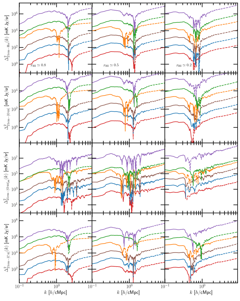
Figure 14: Cross-correlation functions between 21 cm and H $\alpha$ (top row), [O iii] (second row), [O iii] ₈₈ (third row) and [C ii] (fourth row) at volume weighted neutral fractions of $0.8$ (left panels), $0.5$ (middle panels) and $0.2$ (right panels). The different coloured lines indicate the different simulations in our suite, namely, thesan-1 (red curves), thesan-2 (blue curves), thesan-wc-2 (brown curves), thesan-high-2 (orange curves), thesan-low-2 (green curves) and thesan-sdao-2 (purple curves). The lines are offset by regular intervals (a factor of 10 between each simulation) in order to improve clarity by preventing the lines from overlapping with each other.

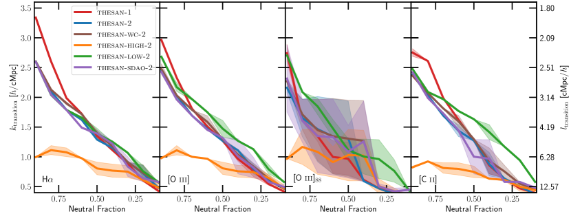
Figure 15: The transition wavenumber ($k_{\mathrm{transition}}$; left axis) and the corresponding transition scale ($l_{\mathrm{transition}}$; right axis) as a function of the volume-weighted neutral fraction in the Universe for the various emission lines and reionization models as indicated. While the general picture of $k_{\mathrm{transition}}$ decreasing as reionization progresses is valid, its exact value and evolution depends substantially on the reionization model and to a lesser extent on the emission line. The simulations in which high mass haloes dominate the ionizing photon budget consistently show lower values of $k_{\mathrm{transition}}$ and vice versa.

3.4 Cross-correlation spectra

In Figure 13 we show the cross-correlation PS between the 21 cm emission and H $\alpha$ emission in thesan-1. The cross-correlation PS between two emission line intensity distributions $I_{1}(x)$ and $I_{2}(x)$ is defined as

$$\Delta^{2}_{I_{1}-I_{2}}(k)=\frac{k^{3}}{2\pi^{2}}\frac{\left<\mathrm{Re}(\tilde{I}_{1})\mathrm{Re}(\tilde{I}_{2})+\mathrm{Im}(\tilde{I}_{1})\mathrm{Im}(\tilde{I}_{2})\right>}{V_{\mathrm{box}}}~{},$$ (4)

where $\tilde{I}(k)$ is the Fourier transform of $I(x)$ and Re$(\tilde{I})$ and Im$(\tilde{I})$ denote the real and Imaginary parts of $\tilde{I}(k)$ respectively. The colours indicate the volume weighted ionization fractions ranging from $0.1$–$0.9$, in increments of $0.1$. A positive correlation between the quantities is indicated by a dashed curve while the solid curves signal a negative correlation. In the initial stages of the reionization process ($x_{\text{H\,{ii}}}\lesssim 0.1$), both the small and the large scale fluctuations correlate positively. The positive correlation on small scales can be explained by the fact that both the H $\alpha$ emission and the neutral hydrogen gas exists in the high density filaments and knots that host galaxies. On the largest scales, both emission line maps follow the underlying matter density distribution. They are anti-correlated on intermediate scales ($0.9\lesssim k\,\mathrm{[}h\mathrm{/cMpc}\mathrm{]}\lesssim 4$), reflecting the relatively small sizes of these early H ii regions. By $x_{\text{H\,{ii}}}\sim 0.2$, the bubbles grow large enough that all the large scale modes ($k\,\mathrm{[}h\mathrm{/cMpc}\mathrm{]}\lesssim 3$) are anti-correlated. We note that even smaller wavenumbers might still be positively correlated, but the simulated volume is not large enough to capture these scales. As the bubble sizes increase, the point at which the cross-correlation PS switches sign, known as the transition wavenumber ($k_{\mathrm{transition}}$), moves to larger and larger spatial scales. Eventually all the spatial scales will show a positive correlation because the only neutral gas in the Universe will be present in the high density regions that also host galaxies that are the sites for H $\alpha$ emission. $k_{\mathrm{transition}}$ can therefore be used to inform us about the progress of reionization and the neutral fraction evolution (Gong et al., 2012).

Of course, the exact value of the transition wavenumber will depend on the topology of the ionized bubbles and to a lesser extent on the underlying nebular emission line distribution. Therefore, the value of $k_{\mathrm{transition}}$ and its evolution with redshift will allow us to place constraints on the sources responsible for the reionization process (Dumitru et al., 2019). In Figure 14 we plot the cross-correlation functions at volume weighted neutral fractions of $0.8$, $0.5$ and $0.2$, between 21 cm and H $\alpha$, [O iii], [O iii] ₈₈ and [C ii] as indicated. The different coloured lines indicate the different simulations in our suite, namely, thesan-1 (red curves), thesan-2 (blue curves), thesan-wc-2 (brown curves), thesan-high-2 (orange curves), thesan-low-2 (green curves) and thesan-sdao-2 (purple curves). All reionization models show a relatively large $k_{\mathrm{transition}}$ at low ionization fractions and decrease as the bubble sizes increase. However, the exact value $k_{\mathrm{transition}}$ and its evolution with the neutral fraction evolution is model dependent. Since thesan-high-2 has the largest bubble sizes for a given ionization fraction, the transition happens at smaller wavenumbers when compared to other models. thesan-low-2, on the other hand, generally shows the largest $k_{\mathrm{transition}}$, except at very low ionization fractions, where thesan-1 shows the largest $k_{\mathrm{transition}}$ because haloes at the very low mass end contribute the most during the initial stages of reionization. These haloes do not contribute in the other simulations, because they are not well resolved, thereby artificially reducing their star-formation rates.

In Figure 15 we further quantify this behaviour by plotting $k_{\mathrm{transition}}$ as a function of the volume weighted neutral fraction in the different simulations and for the different lines, as indicated. The shaded regions denote the uncertainty in $k_{\mathrm{transition}}$ arising from the fact that the transition is not sharp because the cross-correlation function fluctuates between positive and negative values before switching sign permanently. $k_{\mathrm{transition}}$ is calculated as the mean of the smallest value of $k$ where the function is positive and the largest value of $k$ where it is negative and the uncertainty is just the span between these values. If there is more than one transition point, then we quote the values for the largest $k$. The errors in $k_{\mathrm{transition}}$ are generally quite small, except for the [O iii] ₈₈ line which is shot-noise dominated except for the largest scales.

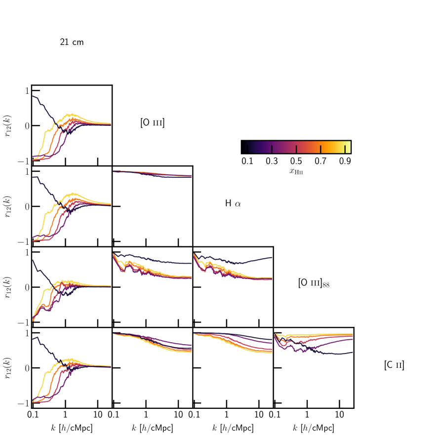
Figure 16: The cross-correlation coefficient ($r_{12}$; defined in Eq. 5) as a function of the wavenumber for the different emission lines considered in this work. The two intensity maps will be perfectly correlated or anti-correlated if $r_{12}(k)=1\,\mathrm{or}\,-1$, respectively. Values close to zero indicate de-correlation between the lines. H $\alpha$, [O iii] and [C ii] are well-correlated with each other on most spatial scales, while the steeper slope of the far IR line [O iii] ₈₈ makes it de-correlate rapidly at smaller $k$.

The general picture of $k_{\mathrm{transition}}$ decreasing as reionization progresses is valid for all models and all the lines considered in this work. However, the exact value and its evolution depends heavily on the reionization model and to a lesser extent on the emission line. thesan-high-2 shows the smallest $k_{\mathrm{transition}}$ for all the lines considered at all neutral fractions, mirroring the fact that this reionization model has the highest contribution from large bubble sizes at any given ionization fraction (see Section 3.4 of Kannan et al., 2022). The slope of the relation is quite shallow with $k_{\mathrm{transition}}$ only changing by a factor of 2 over the majority of the reionization history. All the other simulations show a much steeper slope (with values changing by more than a factor of $5$), with thesan-1 showing the steepest. This is because the initial stages of reionization are dominated by the very low mass haloes ($10^{8}$–$10^{9}$ M_⊙) that are essentially unresolved in the other, lower resolution simulations. thesan-low-2 generally shows higher $k_{\mathrm{transition}}$ when compared to other models because low bubble sizes dominate the reionization process. While this general picture is true for all emission lines considered in this work, there are slight differences in the exact value of $k_{\mathrm{transition}}$ that might help place constraints on the slope of the $L$–$\mathrm{SFR}$ relation for the different lines. It is therefore quite clear that the value of the transition wavenumber and its evolution provide important information that can help place stringent constraints on the bubble size distribution, which in turn informs us about the sources that dominate the ionizing photon budget at any particular redshift.

Finally, in Figure 16 we show the scale dependant correlation coefficient, $r_{12}(k)$, in thesan-1 between 21 cm and different nebular emission lines considered in this work for $x_{\text{H\,{ii}}}=0.1$–$0.9$ in increments of $0.2$ as indicated. This quantifies the amount of correlation between the two intensity maps and is defined as

$$r_{12}(k)=\frac{P_{12}(k)}{\sqrt{P_{11}(k)P_{22}(k)}}~{},$$ (5)

where $P_{12}(k)$ is the cross-correlation PS and $P_{11}(k)$ and $P_{22}(k)$ are the corresponding auto-correlation spectra. The two intensity maps will be perfectly correlated or anti-correlated if $r_{12}(k)=1\,\mathrm{or}\,-1$, respectively. Values close to zero indicate de-correlation between the lines. In general, the closer the slopes of the $L$–$\mathrm{SFR}$ relation the more correlated the nebular emission lines will be. It is important to quantify the cross-correlation coefficient because the auto-spectrum can be estimated from cross-spectra (Beane et al., 2019). This technique is more robust to residual foregrounds than the usual 21 cm auto-power spectrum measurements and can help in verifying auto-spectrum detections. In fact, the larger the number of emission lines used the better the estimate of the spectrum. Importantly, $r_{12}$ also determines the ability to use one line as a tracer of the other, in order to subtract foregrounds/interlopers (Schaan & White, 2021), with values near one indicating good subtraction while values near zero indicate ineffective subtraction. Moreover, since the lines considered in this paper all trace slightly different gas phases in the ISM of star-forming galaxies, the correlated abundance of these lines can help constrain the ISM of high-redshift galaxies (Sun et al., 2019).

Mirroring Figure 14, cross-correlation coefficients between the 21 cm emission and nebular emission lines show positive values at large scales in the initial stages of reionization. The intermediate wavenumbers are negatively correlated and the smallest scales are decorrelated. This picture changes rapidly, with most of the large spatial scales anti-correlating with the nebular emission lines by $x_{\text{H\,{ii}}}\gtrsim 0.3$. The optical emission lines are well correlated ($r_{12}>0.8$) with each other on most spatial scales. However, the steeper slope of the far IR line [O iii] ₈₈ means that it only correlates with the optical lines on the largest scales and $r_{12}$ decreases steeply with $k$. The larger the difference between the slopes of the two luminosity relations, the more quickly the lines de-correlate. Since the slope of the [C ii] line matches the slope of the optical lines, it correlates well with them. Interestingly, the changing slope with redshift causes the line to de-correlate more with decreasing redshift (increased ionized fraction), which suggests that there is complementary information to be obtained by joint analyses of multiple emission lines.

4 Discussion and Conclusions

In this work we have presented a self-consistent framework to predict the intensity maps of a variety of nebular emission lines emanating from reionization era galaxies using the state-of-the-art thesan simulations. The spectral energy distributions including the nebular emission line properties of the simulated galaxies are derived by interpolating between a grid of photo-ionization calculations using the cloudy code as described in Byler et al. (2017). Dust attenuation is modelled using the Monte Carlo radiative transfer code skirt (last described in Camps & Baes, 2020), with the dust mass in each cell determined by a spatially constant dust to metal ratio (DTM) that was derived to match the observed UV luminosity function evolution from $z=2$–$10$ (Vogelsberger et al., 2020b). The main results and conclusions of this work are as follows:

1. We construct dust-attenuated SEDs for all well-resolved galaxies in the thesan-1 simulation. The derived UV magnitudes match the observationally inferred luminosity function over a wide range of magnitudes. They are also in broad agreement with the $M_{\star}$–$M_{\mathrm{UV}}$ relation and measured UV continuum slope ($\beta_{\mathrm{UV}}$) of high-redshift galaxies.

2. We provide fitting functions for the luminosity–star-formation rate relations ($L$–$\mathrm{SFR}$) of the brightest four rest frame optical emission lines, [O ii] ($3726,3729$ Å), H $\beta$ ($4861$ Å), [O iii] ($4959,5007$ Å) and H $\alpha$ ($6563$ Å), and four fine structure emission lines in the far IR, [O iii] ₅₂ ($52$ µm), [O iii] ₈₈ ($88$ µm), [N ii] ($122$ µm) and [C ii] ($158$ µm).

3. We determine that important differences exist between the derived $L$–$\mathrm{SFR}$ relation for high-$z$ galaxies and the commonly used low-$z$ estimates. Specifically, the hydrogen emission lines show shallower scaling relations and slightly higher amplitudes, while the metal lines show steeper slopes with generally lower amplitudes. These differences can be attributed to the fact that high-$z$ galaxies are generally less metal enriched than their low-$z$ counterparts.

4. Our predicted mean intensities of the Balmer emission lines are about a factor of $3-4$ larger than previous estimates (see for example, Gong et al., 2017). This disparity is mostly due to the higher LyC production rate in low metallicity stars efficiently forming within lower-mass haloes, which was not accounted for in previous works.

5. We show that the cross-correlation power spectra between the 21 cm emission and various nebular emission lines can be used to infer the evolution of the neutral hydrogen fraction during reionization. The scale at which the cross-correlation PS switches sign, knows as the transition wavenumber ($k_{\mathrm{transition}}$), moves to larger spatial scales as reionization progresses.

6. The value of $k_{\mathrm{transition}}$ and its evolution depend strongly on the reionization model and to a lesser extent on the emission line considered. Scenarios in which massive haloes dominate the ionizing photon budget show consistently lower values of $k_{\mathrm{transition}}$ and vice-versa. This is consistent with the picture that the transition scale probes the typical sizes of ionized regions.

7. The cross-correlation coefficients show that the nebular emission lines H $\alpha$, [O iii] and [C ii] are well-correlated with each other on most spatial scales. However, the steeper slope of the far IR line [O iii] ₈₈ means that it only correlates with the other lines on the largest scales and de-correlates rapidly at smaller spatial scales, where shot noise dominates.

The emission line modelling presented in this work does a relatively good job of estimating the luminosities of the lines arising from highly ionized H ii regions around newly formed young stars. However, it is unable to predict the luminosities of lines which predominantly originate in PDRs such as [C ii] ($158$ µm) and [O i] ($63$ µm). Accurate modelling of these lines will require additional assumptions about the prevalence and distribution of giant molecular clouds and the spatial distribution of the far-UV radiation field (Olsen et al., 2015, 2017). In a similar vein, line luminosities of the various CO lines would require assumptions about the molecular gas fractions within galaxies. While scaling relations like the ones presented in Leroy et al. (2008) and Gnedin & Draine (2014) can be used to estimate the molecular gas content, they usually rely on the physics of low redshift, high metallicity galaxies, where the main H ₂ formation channel is via dust grains. This approximation is unlikely to be accurate in low metallicity environments where a series of gas phase reactions involving intermediary ions like H ^- and H ${}^{+}_{2}$ are the primary channels for molecular gas formation (Glover, 2005). Thus, self-consistent CO LIM predictions would ideally require more rigorous modelling of the multi-phase ISM coupled with molecular thermochemistry and radiation field intensities (Katz et al., 2019; Kannan et al., 2020), which we leave for future work.

Beyond this, the prominent Ly $\alpha$ transition ($2$–$1$) of neutral hydrogen is an exceptionally promising target for upcoming intensity mapping experiments like SPHEREx and CDIM (e.g. Visbal & McQuinn, 2018; Mas-Ribas & Chang, 2020). Part of the utility of Ly $\alpha$ stems from the additional physics of resonant absorption, which effectively removes Ly $\alpha$ photons out of the line of sight to be lost to the diffuse cosmic optical and infrared backgrounds (Gunn & Peterson, 1965). This encodes information about both the sources (galaxies) and sinks (IGM) for a powerful probe of reionization, e.g. Ly $\alpha$ emitting galaxies (LAEs) and the Ly $\alpha$ forest in emission and absorption, respectively (in the context of thesan, see Garaldi et al., 2022; Smith et al., 2022). However, in practice the theoretical modelling and observational interpretations are both significantly more complex because the results are highly sensitive to the radiative transfer within galaxies and through the intervening IGM (Dijkstra, 2019; Ouchi et al., 2020). In particular, the emergent Ly $\alpha$ spectral flux from high-$z$ galaxies is very sensitive to neutral hydrogen and dust column densities, feedback regulated outflows and morphologies, and time and anisotropy variability, all of which increase the uncertainty of modelling Ly $\alpha$ properties during the Epoch of Reionization with important consequences for Ly $\alpha$ LIM as well (e.g. Smith et al., 2017, 2019; Behrens et al., 2019; Laursen et al., 2019; Garel et al., 2021). In a future accompanying paper (Smith et al. in prep.) we will provide Ly $\alpha$ intensity mapping predictions based on high time cadence on-the-fly redshift-space renderings of Ly $\alpha$ properties. In combination with insights from detailed Monte Carlo Ly $\alpha$ radiative transfer simulations and IGM transmission studies, we hope to similarly advance our understanding of Ly $\alpha$ LIM theory, modelling, and interpretation.

Multi-tracer line intensity mapping, by nature, requires a variety of observational instruments to measure lines at different wavelengths, each with its own sensitivity and instrument-specific noise power spectrum. Moreover, the signal-to-noise ratios depend on cost optimisations such as beam sizes and integration times. Therefore, placing constraints on any astrophysical and cosmological parameters would require an intimate knowledge of these instrumental effects, survey strategies, and realistic signal contaminants. We therefore choose to defer predictions for the detectability of the various lines and the constraining power of these measurements to a future paper. We hope that the emission line scaling relations and predictions for the line intensity maps derived in this work will provide a rigorous theoretical framework upon which the results from current and upcoming LIM experiments can be analysed and interpreted.

Data Availability

All simulation data, including intrinsic and dust attenuated galaxy SEDs will be made publicly available in the near future. Data will be distributed via www.thesan-project.com. Before the public data release, data underlying this article will be shared on reasonable request to the corresponding author(s).

Appendix A Extrapolation convergence

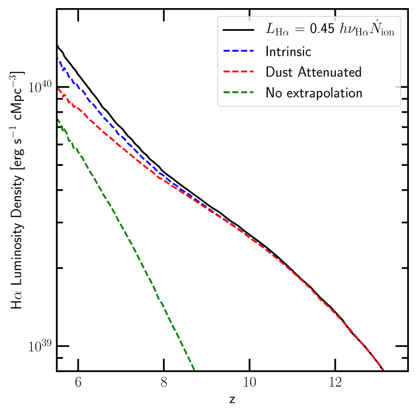
Figure 17: The theoretically calculated H $\alpha$ luminosity density as a function of redshift (black curve) compared to the H $\alpha$ luminosity values obtained from using the $L$–$\mathrm{SFR}$ fitting relation derived from intrinsic (blue curve) and dust-attenuated SEDs (red curve). For comparison the green curve plots the H $\alpha$ luminosity if only the values from well-resolved haloes (as defined in Section 2) are considered. The fact that the extrapolated H $\alpha$ luminosities are close to the theoretically expected values, especially at high redshifts, shows the goodness of the fits and the effectiveness of extrapolating the fits to all haloes in the simulation.

One of the major assumptions in our model is that the $L$–$\mathrm{SFR}$ fits derived from the emission line calculations of the well-resolved galaxies (as defined in Section 2) are also valid for the lower-mass galaxies in the simulation volume. We test the validity of this extrapolation by comparing the H $\alpha$ luminosity density derived from the $L$–$\mathrm{SFR}$ fits applied to all galaxies in the simulation volume to the theoretically expected value as shown in Figure 17. The theoretical value is derived by assuming that all LyC photons in the simulation lead to the ionization of a hydrogen atom. These atoms recombine leading to H $\alpha$ line emission with a conversion probability per recombination event of $0.45$ (black curve). The total LyC production rate is calculated by summing up the ionizing emissivity of all the stars in the simulation volume. For comparison, the plot also shows the H $\alpha$ luminosity density obtained from using the $L$–$\mathrm{SFR}$ fitting relation derived from intrinsic (defined as the sinlge power law relation with slope $m_{a}$ and intercept $a$ as described by Eq. 1; blue curve) and dust-attenuated SEDs (red curve). Finally, the green curve plots the luminosity if only the well-resolved haloes are considered. The fact that the extrapolated H $\alpha$ luminosities are close to the theoretically expected values, especially at high redshifts, shows the reliability of the fits and the effectiveness of extrapolating the fits to all haloes in the simulation. We note that the decrease in the H $\alpha$ luminosity at low-$z$ is due to dust attenuation, which becomes increasingly important at lower redshifts. The discrepancy between the theoretical and intrinsic fits arises from the fact that at low-$z$, the ISM becomes more metal enriched, meaning that a larger fraction of the ionizing photons is used up for ionizing metals rather than hydrogen.

Appendix B Dependence of $k_{\mathrm{transition}}$ on the slope of the $L$–$\mathrm{SFR}$ relation

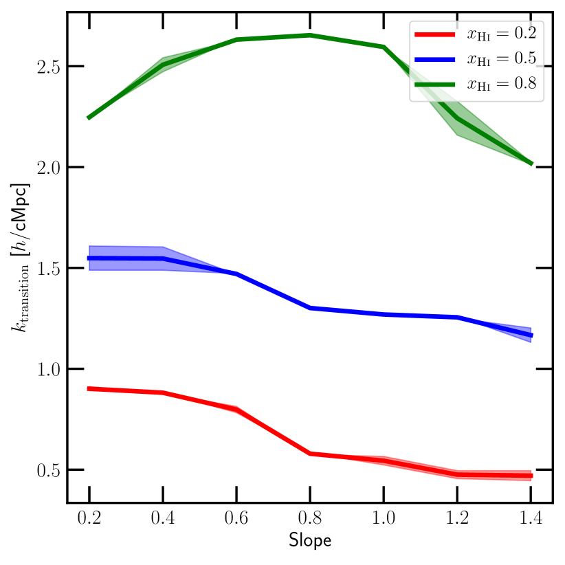
Figure 18: The value of $k_{\mathrm{transition}}$ as a function of the slope of the $L$–$\mathrm{SFR}$ relation at three different neutral fractions of $x_{\text{H\,{i}}}=0.2$ (red curve), $x_{\text{H\,{i}}}=0.5$ (blue curve), and $x_{\text{H\,{i}}}=0.8$ (green curve) in the thesan-1 simulation. While $k_{\mathrm{transition}}$ generally traces the reionization history, there is a non-negligible dependence on the slope of the $L$–$\mathrm{SFR}$ relation. It is therefore important to accurately model the $L$–$\mathrm{SFR}$ relation in order to reliably constrain the reionization history of the Universe using cross-correlation spectra.

The value of $k_{\mathrm{transition}}$ is usually assumed to trace the average scale of the ionized bubble during the reionization process (Dumitru et al., 2019), with the impact of the slope of the $L$–$\mathrm{SFR}$ relation assumed to be minimal. Here we test this hypothesis by changing the slope of $L$–$\mathrm{SFR}$ relation from $0.2$–$1.4$ and cross-correlating with the 21 cm filed at three different values for the ionization fractions as indicated in Figure 18. We note that for slopes of $m\gtrsim 1$, the highest luminosity galaxies start to dominate the total emission luminosity in the line, reducing the significance of the fluctuations arising from lower luminosity haloes. This leads to an increase in shot noise contribution even at relatively larger spatial scales. We therefore, choose to cap the slope at the high SFR end ($x_{c}$ in Eq. 1) to $0.8$. This is equivalent to masking out the most luminous haloes in the volume so as to highlight the lower luminosity features in the LIM. As expected $k_{\mathrm{transition}}$ shows a strong dependence on the ionization fraction, in agreement with the picture that it traces the average size of the ionized regions. Nonetheless, there is a non-negligible dependence on the slope of the $L$–$\mathrm{SFR}$ relation. It is therefore important to accurately model the $L$–$\mathrm{SFR}$ relation in order to reliably constrain the reionization history of the Universe using cross-correlation spectra. However, we do note that the slope of the $L$–$\mathrm{SFR}$ relation has to be really poorly constrained in order for it to produce an appreciable uncertainty in $k_{\mathrm{transition}}$. If the slope is constrained within a factor of $0.2$, then the uncertainty in $k_{\mathrm{transition}}$ is pretty small, and this quantity can therefore be used as a rigorous probe of the reionization process.

References

- Aoyama et al. (2017) Aoyama S., Hou K.-C., Shimizu I., Hirashita H., Todoroki K., Choi J.-H., Nagamine K., 2017, MNRAS, 466, 105
- Arata et al. (2020) Arata S., Yajima H., Nagamine K., Abe M., Khochfar S., 2020, MNRAS, 498, 5541
- Atek et al. (2018) Atek H., Richard J., Kneib J.-P., Schaerer D., 2018, MNRAS, 479, 5184
- Bagnasco et al. (2007) Bagnasco G., et al., 2007, in Heaney J. B., Burriesci L. G., eds, Society of Photo-Optical Instrumentation Engineers (SPIE) Conference Series Vol. 6692, Cryogenic Optical Systems and Instruments XII. p. 66920M, doi:10.1117/12.735602
- Baldwin et al. (1981) Baldwin J. A., Phillips M. M., Terlevich R., 1981, PASP, 93, 5
- Barnes & Hut (1986) Barnes J., Hut P., 1986, Nature, 324, 446
- Beane et al. (2019) Beane A., Villaescusa-Navarro F., Lidz A., 2019, ApJ, 874, 133
- Behrens et al. (2019) Behrens C., Pallottini A., Ferrara A., Gallerani S., Vallini L., 2019, MNRAS, 486, 2197
- Bekki (2015) Bekki K., 2015, MNRAS, 449, 1625
- Bhatawdekar & Conselice (2021) Bhatawdekar R., Conselice C. J., 2021, ApJ, 909, 144
- Bhatawdekar et al. (2019) Bhatawdekar R., Conselice C. J., Margalef-Bentabol B., Duncan K., 2019, MNRAS, 486, 3805
- Bouwens et al. (2014) Bouwens R. J., et al., 2014, ApJ, 793, 115
- Bouwens et al. (2015) Bouwens R. J., et al., 2015, ApJ, 803, 34
- Bouwens et al. (2017) Bouwens R. J., Oesch P. A., Illingworth G. D., Ellis R. S., Stefanon M., 2017, ApJ, 843, 129
- Byler et al. (2017) Byler N., Dalcanton J. J., Conroy C., Johnson B. D., 2017, ApJ, 840, 44
- Byler et al. (2018) Byler N., Dalcanton J. J., Conroy C., Johnson B. D., Levesque E. M., Berg D. A., 2018, ApJ, 863, 14
- CCAT-Prime collaboration et al. (2021) CCAT-Prime collaboration et al., 2021, arXiv e-prints, p. arXiv:2107.10364
- Calzetti et al. (1994) Calzetti D., Kinney A. L., Storchi-Bergmann T., 1994, ApJ, 429, 582
- Camps & Baes (2020) Camps P., Baes M., 2020, Astronomy and Computing, 31, 100381
- Chabrier (2003) Chabrier G., 2003, PASP, 115, 763
- Cleary et al. (2016) Cleary K., et al., 2016, in American Astronomical Society Meeting Abstracts #227. p. 426.06
- Conroy et al. (2009) Conroy C., Gunn J. E., White M., 2009, ApJ, 699, 486
- Cooray et al. (2019) Cooray A., et al., 2019, in Bulletin of the American Astronomical Society. p. 23 (arXiv:1903.03144)
- De Cia et al. (2016) De Cia A., Ledoux C., Mattsson L., Petitjean P., Srianand R., Gavignaud I., Jenkins E. B., 2016, A&A, 596, A97
- De Looze et al. (2014) De Looze I., et al., 2014, A&A, 568, A62
- DeBoer et al. (2017) DeBoer D. R., et al., 2017, PASP, 129, 045001
- Dijkstra (2019) Dijkstra M., 2019, Saas-Fee Advanced Course, 46, 1
- Doré et al. (2014) Doré O., et al., 2014, arXiv e-prints, p. arXiv:1412.4872
- Draine & Li (2007) Draine B. T., Li A., 2007, ApJ, 657, 810
- Driver et al. (2013) Driver S. P., Robotham A. S. G., Bland-Hawthorn J., Brown M., Hopkins A., Liske J., Phillipps S., Wilkins S., 2013, MNRAS, 430, 2622
- Dumitru et al. (2019) Dumitru S., Kulkarni G., Lagache G., Haehnelt M. G., 2019, MNRAS, 485, 3486
- Eldridge et al. (2017) Eldridge J. J., Stanway E. R., Xiao L., McClelland L. A. S., Taylor G., Ng M., Greis S. M. L., Bray J. C., 2017, Publ. Astron. Soc. Australia, 34, e058
- Ewen & Purcell (1951) Ewen H. I., Purcell E. M., 1951, Nature, 168, 356
- Ferkinhoff et al. (2010) Ferkinhoff C., Hailey-Dunsheath S., Nikola T., Parshley S. C., Stacey G. J., Benford D. J., Staguhn J. G., 2010, ApJ, 714, L147
- Ferkinhoff et al. (2011) Ferkinhoff C., et al., 2011, ApJ, 740, L29
- Ferland et al. (2017) Ferland G. J., et al., 2017, Rev. Mex. Astron. Astrofis., 53, 385
- Finkelstein et al. (2015) Finkelstein S. L., et al., 2015, ApJ, 810, 71
- Fonseca et al. (2017) Fonseca J., Silva M. B., Santos M. G., Cooray A., 2017, MNRAS, 464, 1948
- Garaldi et al. (2022) Garaldi E., Kannan R., Smith A., Springel V., Pakmor R., Vogelsberger M., Hernquist L., 2022, MNRAS, 512, 4909
- Garel et al. (2021) Garel T., Blaizot J., Rosdahl J., Michel-Dansac L., Haehnelt M. G., Katz H., Kimm T., Verhamme A., 2021, MNRAS, 504, 1902
- Glover (2005) Glover S., 2005, Space Sci. Rev., 117, 445
- Gnedin (2014) Gnedin N. Y., 2014, ApJ, 793, 29
- Gnedin & Draine (2014) Gnedin N. Y., Draine B. T., 2014, ApJ, 795, 37
- Gong et al. (2012) Gong Y., Cooray A., Silva M., Santos M. G., Bock J., Bradford C. M., Zemcov M., 2012, ApJ, 745, 49
- Gong et al. (2017) Gong Y., Cooray A., Silva M. B., Zemcov M., Feng C., Santos M. G., Dore O., Chen X., 2017, ApJ, 835, 273
- Greig et al. (2017) Greig B., Mesinger A., Haiman Z., Simcoe R. A., 2017, MNRAS, 466, 4239
- Gunn & Peterson (1965) Gunn J. E., Peterson B. A., 1965, ApJ, 142, 1633
- Hashimoto et al. (2018) Hashimoto T., et al., 2018, Nature, 557, 392
- Hassan et al. (2021) Hassan S., Davé R., McQuinn M., Somerville R. S., Keating L. C., Anglés-Alcázar D., Villaescusa-Navarro F., Spergel D. N., 2021, arXiv e-prints, p. arXiv:2109.03840
- Heneka & Cooray (2021) Heneka C., Cooray A., 2021, MNRAS, 506, 1573
- Hirschmann et al. (2017) Hirschmann M., Charlot S., Feltre A., Naab T., Choi E., Ostriker J. P., Somerville R. S., 2017, MNRAS, 472, 2468
- Hirschmann et al. (2019) Hirschmann M., Charlot S., Feltre A., Naab T., Somerville R. S., Choi E., 2019, MNRAS, 487, 333
- Iliev et al. (2014) Iliev I. T., Mellema G., Ahn K., Shapiro P. R., Mao Y., Pen U.-L., 2014, MNRAS, 439, 725
- Inoue (2003) Inoue A. K., 2003, PASJ, 55, 901
- Ishigaki et al. (2018) Ishigaki M., Kawamata R., Ouchi M., Oguri M., Shimasaku K., Ono Y., 2018, ApJ, 854, 73
- Jonsson et al. (2010) Jonsson P., Groves B. A., Cox T. J., 2010, MNRAS, 403, 17
- Kannan et al. (2019) Kannan R., Vogelsberger M., Marinacci F., McKinnon R., Pakmor R., Springel V., 2019, MNRAS, 485, 117
- Kannan et al. (2020) Kannan R., Marinacci F., Vogelsberger M., Sales L. V., Torrey P., Springel V., Hernquist L., 2020, MNRAS, 499, 5732
- Kannan et al. (2021) Kannan R., Vogelsberger M., Marinacci F., Sales L. V., Torrey P., Hernquist L., 2021, MNRAS, 503, 336
- Kannan et al. (2022) Kannan R., Garaldi E., Smith A., Pakmor R., Springel V., Vogelsberger M., Hernquist L., 2022, MNRAS, 511, 4005
- Katz et al. (2019) Katz H., et al., 2019, MNRAS, 487, 5902
- Kaurov & Gnedin (2016) Kaurov A. A., Gnedin N. Y., 2016, ApJ, 824, 114
- Kennicutt (1998) Kennicutt Robert C. J., 1998, ARA&A, 36, 189
- Kewley et al. (2013) Kewley L. J., Dopita M. A., Leitherer C., Davé R., Yuan T., Allen M., Groves B., Sutherland R., 2013, ApJ, 774, 100
- Kewley et al. (2019) Kewley L. J., Nicholls D. C., Sutherland R. S., 2019, ARA&A, 57, 511
- Kovetz et al. (2017) Kovetz E. D., et al., 2017, arXiv e-prints, p. arXiv:1709.09066
- Kovetz et al. (2019) Kovetz E., et al., 2019, BAAS, 51, 101
- Kroupa (2001) Kroupa P., 2001, MNRAS, 322, 231
- Lagache et al. (2018) Lagache G., Cousin M., Chatzikos M., 2018, A&A, 609, A130
- Laursen et al. (2019) Laursen P., Sommer-Larsen J., Milvang-Jensen B., Fynbo J. P. U., Razoumov A. O., 2019, A&A, 627, A84
- Leja et al. (2017) Leja J., Johnson B. D., Conroy C., van Dokkum P. G., Byler N., 2017, ApJ, 837, 170
- Leroy et al. (2008) Leroy A. K., Walter F., Brinks E., Bigiel F., de Blok W. J. G., Madore B., Thornley M. D., 2008, AJ, 136, 2782
- Leung et al. (2020) Leung T. K. D., Olsen K. P., Somerville R. S., Davé R., Greve T. R., Hayward C. C., Narayanan D., Popping G., 2020, ApJ, 905, 102
- Levermore (1984) Levermore C. D., 1984, J. Quant. Spectrosc. Radiative Transfer, 31, 149
- Lidz et al. (2011) Lidz A., Furlanetto S. R., Oh S. P., Aguirre J., Chang T.-C., Doré O., Pritchard J. R., 2011, ApJ, 741, 70
- Livermore et al. (2017) Livermore R. C., Finkelstein S. L., Lotz J. M., 2017, ApJ, 835, 113
- Lupi et al. (2020) Lupi A., Pallottini A., Ferrara A., Bovino S., Carniani S., Vallini L., 2020, MNRAS, 496, 5160
- Lusso et al. (2015) Lusso E., Worseck G., Hennawi J. F., Prochaska J. X., Vignali C., Stern J., O’Meara J. M., 2015, MNRAS, 449, 4204
- Ly et al. (2007) Ly C., et al., 2007, ApJ, 657, 738
- Madau & Dickinson (2014) Madau P., Dickinson M., 2014, ARA&A, 52, 415
- Maiolino et al. (2015) Maiolino R., et al., 2015, MNRAS, 452, 54
- Mao et al. (2012) Mao Y., Shapiro P. R., Mellema G., Iliev I. T., Koda J., Ahn K., 2012, MNRAS, 422, 926
- Marinacci et al. (2018) Marinacci F., et al., 2018, MNRAS, 480, 5113
- Mas-Ribas & Chang (2020) Mas-Ribas L., Chang T.-C., 2020, Phys. Rev. D, 101, 083032
- McKinnon et al. (2016) McKinnon R., Torrey P., Vogelsberger M., 2016, MNRAS, 457, 3775
- McKinnon et al. (2017) McKinnon R., Torrey P., Vogelsberger M., Hayward C. C., Marinacci F., 2017, MNRAS, 468, 1505
- McLeod et al. (2016) McLeod D. J., McLure R. J., Dunlop J. S., 2016, MNRAS, 459, 3812
- Mellema et al. (2013) Mellema G., et al., 2013, Experimental Astronomy, 36, 235
- Naiman et al. (2018) Naiman J. P., et al., 2018, MNRAS, 477, 1206
- Nelson et al. (2018) Nelson D., et al., 2018, MNRAS, 475, 624
- Olsen et al. (2015) Olsen K. P., Greve T. R., Narayanan D., Thompson R., Toft S., Brinch C., 2015, ApJ, 814, 76
- Olsen et al. (2017) Olsen K., Greve T. R., Narayanan D., Thompson R., Davé R., Niebla Rios L., Stawinski S., 2017, ApJ, 846, 105
- Osterbrock & Ferland (2006) Osterbrock D. E., Ferland G. J., 2006, Astrophysics of gaseous nebulae and active galactic nuclei
- Ouchi et al. (2013) Ouchi M., et al., 2013, ApJ, 778, 102
- Ouchi et al. (2020) Ouchi M., Ono Y., Shibuya T., 2020, ARA&A, 58, 617
- Pakmor & Springel (2013) Pakmor R., Springel V., 2013, MNRAS, 432, 176
- Pallottini et al. (2019) Pallottini A., et al., 2019, MNRAS, 487, 1689
- Parsons et al. (2010) Parsons A. R., et al., 2010, AJ, 139, 1468
- Pillepich et al. (2018a) Pillepich A., et al., 2018a, MNRAS, 473, 4077
- Pillepich et al. (2018b) Pillepich A., et al., 2018b, MNRAS, 475, 648
- Planck Collaboration et al. (2016) Planck Collaboration et al., 2016, A&A, 594, A13
- Powell et al. (1999) Powell K. G., Roe P. L., Linde T. J., Gombosi T. I., De Zeeuw D. L., 1999, Journal of Computational Physics, 154, 284
- Qin et al. (2022) Qin W., Schutz K., Smith A., Garaldi E., Kannan R., Slatyer T. R., Vogelsberger M., 2022, arXiv e-prints, p. arXiv:2205.06270
- Reddy et al. (2012) Reddy N., et al., 2012, ApJ, 744, 154
- Rémy-Ruyer et al. (2014) Rémy-Ruyer A., et al., 2014, A&A, 563, A31
- Rigopoulou et al. (2018) Rigopoulou D., Pereira-Santaella M., Magdis G. E., Cooray A., Farrah D., Marques-Chaves R., Perez-Fournon I., Riechers D., 2018, MNRAS, 473, 20
- Rybicki & Lightman (1986) Rybicki G. B., Lightman A. P., 1986, Radiative Processes in Astrophysics
- Salpeter (1955) Salpeter E. E., 1955, ApJ, 121, 161
- Schaan & White (2021) Schaan E., White M., 2021, J. Cosmology Astropart. Phys., 2021, 068
- Schaye et al. (2015) Schaye J., et al., 2015, MNRAS, 446, 521
- Shen et al. (2020) Shen X., et al., 2020, MNRAS, 495, 4747
- Shen et al. (2022) Shen X., Vogelsberger M., Nelson D., Tacchella S., Hernquist L., Springel V., Marinacci F., Torrey P., 2022, MNRAS, 510, 5560
- Smith et al. (2017) Smith A., Bromm V., Loeb A., 2017, MNRAS, 464, 2963
- Smith et al. (2019) Smith A., Ma X., Bromm V., Finkelstein S. L., Hopkins P. F., Faucher-Giguère C.-A., Kereš D., 2019, MNRAS, 484, 39
- Smith et al. (2022) Smith A., Kannan R., Garaldi E., Vogelsberger M., Pakmor R., Springel V., Hernquist L., 2022, MNRAS, 512, 3243
- Song et al. (2016) Song M., et al., 2016, ApJ, 825, 5
- Spinoglio et al. (2012) Spinoglio L., Dasyra K. M., Franceschini A., Gruppioni C., Valiante E., Isaak K., 2012, ApJ, 745, 171
- Springel (2010) Springel V., 2010, MNRAS, 401, 791
- Springel & Hernquist (2003) Springel V., Hernquist L., 2003, MNRAS, 339, 289
- Springel et al. (2018) Springel V., et al., 2018, MNRAS, 475, 676
- Springel et al. (2021) Springel V., Pakmor R., Zier O., Reinecke M., 2021, MNRAS, 506, 2871
- Stefanon et al. (2021) Stefanon M., Bouwens R. J., Labbé I., Illingworth G. D., Gonzalez V., Oesch P. A., 2021, ApJ, 922, 29
- Storey & Hummer (1995) Storey P. J., Hummer D. G., 1995, MNRAS, 272, 41
- Sun et al. (2019) Sun G., Hensley B. S., Chang T.-C., Doré O., Serra P., 2019, ApJ, 887, 142
- Vijayan et al. (2021) Vijayan A. P., Lovell C. C., Wilkins S. M., Thomas P. A., Barnes D. J., Irodotou D., Kuusisto J., Roper W. J., 2021, MNRAS, 501, 3289
- Visbal & Loeb (2010) Visbal E., Loeb A., 2010, J. Cosmology Astropart. Phys., 2010, 016
- Visbal & McQuinn (2018) Visbal E., McQuinn M., 2018, ApJ, 863, L6
- Vogelsberger et al. (2013) Vogelsberger M., Genel S., Sijacki D., Torrey P., Springel V., Hernquist L., 2013, MNRAS, 436, 3031
- Vogelsberger et al. (2014) Vogelsberger M., et al., 2014, MNRAS, 444, 1518
- Vogelsberger et al. (2020a) Vogelsberger M., Marinacci F., Torrey P., Puchwein E., 2020a, Nature Reviews Physics, 2, 42
- Vogelsberger et al. (2020b) Vogelsberger M., et al., 2020b, MNRAS, 492, 5167
- Walter et al. (2016) Walter F., et al., 2016, ApJ, 833, 67
- Weinberger et al. (2017) Weinberger R., et al., 2017, MNRAS, 465, 3291
- Weinberger et al. (2018) Weinberger R., et al., 2018, MNRAS, 479, 4056
- Weinberger et al. (2020) Weinberger R., Springel V., Pakmor R., 2020, ApJS, 248, 32
- Wiedner et al. (2020) Wiedner M. C., et al., 2020, arXiv e-prints, p. arXiv:2012.02731
- Wilkins et al. (2013) Wilkins S. M., Bunker A., Coulton W., Croft R., di Matteo T., Khandai N., Feng Y., 2013, MNRAS, 430, 2885
- Wilkins et al. (2020) Wilkins S. M., et al., 2020, MNRAS, 493, 6079
- Wiseman et al. (2017) Wiseman P., Schady P., Bolmer J., Krühler T., Yates R. M., Greiner J., Fynbo J. P. U., 2017, A&A, 599, A24
- Wu et al. (2020) Wu X., Davé R., Tacchella S., Lotz J., 2020, MNRAS, 494, 5636
- Wuyts et al. (2016) Wuyts E., et al., 2016, ApJ, 827, 74
- Yang et al. (2021) Yang S., Lidz A., Popping G., 2021, MNRAS, 504, 723
- Yeh et al. (2022) Yeh J. Y. C., et al., 2022, arXiv e-prints, p. arXiv:2205.02238
- van Haarlem et al. (2013) van Haarlem M. P., et al., 2013, A&A, 556, A2