Orbit determination with the Keplerian integrals

Abstract

We review two initial orbit determination methods for too short arcs (TSAs) of optical observations of a solar system body. These methods employ the conservation laws of Kepler’s problem, and allow to attempt the linkage of TSAs referring to quite far epochs, differing by even more than one orbital period of the observed object. The first method (Link2) concerns the linkage of 2 TSAs, and leads to a univariate polynomial equation of degree 9. An optimal property of this polynomial is proved using Gröbner bases theory. The second method (Link3) is thought for the linkage of 3 TSAs, and leads to a univariate polynomial equation of degree 8. A numerical test is shown for both algorithms.

dedicated to Prof. Andrea Milani

1 Introduction

Modern telescopes collect a very large number of optical observations of solar system bodies, that can be usually grouped in very short arcs (VSAs), see [10]. A VSA is a set

$$\{(\alpha_{i},\delta_{i}),\quad i=1\ldots m\},\qquad m\geq 2$$

of pairs of values of right ascension and declination of the same celestial body, referring to epochs $t_{i}$, and covering a very short path in the sky. Usually the data contained in a VSA do not allow to compute a least squares orbit: in this case we speak of a too short arc (TSA). Given a TSA, we can compute an attributable

$${\cal A}=(\alpha,\delta,\dot{\alpha},\dot{\delta})$$

at the mean epoch $\bar{t}=\frac{1}{m}\sum_{i}t_{i}$ of the observations by a linear or quadratic fit, see [10]. Given an attributable, the radial distance $\rho$ and the radial velocity $\dot{\rho}$ of the observed body remain completely unknown. However, given two attributables referring to the same celestial body, we can try to put them together with the aim of computing an orbit that fits all the data. This operation is called linkage in the orbit determination literature, and it is often challenging: an orbit produced by linking together two TSAs usually needs a confirmation with additional data to be considered reliable. Moreover, we cannot know a priori that two TSAs refer to the same observed body, and to perform an efficient selection of pairs of TSAs to be passed to a linkage algorithm is a critical issue.

In this paper we review two recent initial orbit determination methods, introduced in [4] and [5], for the linkage of two or three TSAs. These are called Link2 and Link3, respectively. Some interesting algebraic aspects of these algorithms are also discussed, and a numerical test is shown for both.

2 Linkage with the Keplerian integrals

The first integrals of Kepler’s motion can be used to write polynomial equations for the linkage of 2 TSAs. The conservation laws of angular momentum and energy were proposed for the linkage problem already in [12], [11], [13]: here the authors observed that the equations could be put in polynomial form but did not use this form, see. A polynomial formulation of the linkage problem was considered later in a series of papers [7], [8], [4]. In [7] the angular momentum and energy conservation laws are used, as in [12]: a polynomial is obtained by squaring twice the equation of the energy conservation. After elimination of variables we get a univariate equation of degree 48 in the radial distance $\rho_{2}$. In [8] the degree is reduced to 20 by using the Laplace-Lenz vector projected along a suitable direction in place of the energy. In [4] all the algebraic conservation laws are combined so that the degree is reduced to 9: this is the algorithm that we recall here.

Remark 1.

Classical preliminary orbit determination methods, e.g. the ones by Gauss, Laplace, Mossotti [3], [9], [1], [6] use the equations of motion, and Taylor series expansions around a central time of the observational arc, thus the observations must necessarily be close enough in time. We observe that using conservation laws this constraint on the time is not required.

2.1 Kepler’s problem and its first integrals

The equation of motion of Kepler’s problem is

$$\ddot{{\bf r}}=-\mu\displaystyle\frac{{\bf r}}{|{\bf r}|^{3}},$$ (1)

where ${\bf r}\in\mathbb{R}^{3}$ is the unknown position vector and $\mu$ is a positive constant. The dynamics defined by (1) has the following conserved quantities:

$${{\bf c}={\bf r}\times\dot{{\bf r}}},\hskip 36.98866pt\mbox{\it angular momentum}$$

$${{\cal E}=\frac{1}{2}|\dot{\bf r}|^{2}-\frac{\mu}{|{\bf r}|}},\hskip 17.07182pt\mbox{\it energy}$$

$${{\bf L}=\frac{1}{\mu}\dot{\bf r}\times{\bf c}-\frac{{\bf r}}{|{\bf r}|}},\hskip 8.5359pt\mbox{\it Laplace-Lenz vector}.$$

We call these quantities the Keplerian integrals. Since ${\bf c}$ and ${\bf L}$ have 3 components we get 7 scalar conserved quantities: among them only 5 are independent, in fact

$${\bf c}\cdot{\bf L}=0,\qquad 2|{\bf c}|^{2}{\cal E}+{\mu}^{2}(1-|{\bf L}|^{2})=0.$$

Given an attributable ${\cal A}$ at the epoch $\bar{t}$, we write below the Keplerian integrals as functions of the unknown radial distance and velocity $\rho,\dot{\rho}$. We start by writing

$$\begin{split}&{\bf r}={\bf q}+\rho\,{\bf e}^{\rho},\cr&\dot{\bf r}=\dot{\bf q}+\dot{\rho}\,{\bf e}^{\rho}+\rho(\dot{\alpha}\cos\delta{\bf e}^{\alpha}+\dot{\delta}{\bf e}^{\delta}),\end{split}$$

where ${\bf q}$, $\dot{\bf q}$ are the position and velocity of the observer at time $\bar{t}$,

$${\bf e}^{\rho}=(\cos\delta\cos\alpha,\cos\delta\sin\alpha,\sin\delta)$$

gives the line of sight, and

$${\bf e}^{\alpha}=(\cos\delta)^{-1}\frac{\partial{\bf e}^{\rho}}{\partial\alpha},\qquad{\bf e}^{\delta}=\frac{\partial{\bf e}^{\rho}}{\partial\delta}.$$

The angular momentum vector can be expressed as

$${\bf c}(\rho,\dot{\rho})={\bf r}\times\dot{{\bf r}}={\bf D}\dot{\rho}+{\bf E}\rho^{2}+{\bf F}\rho+{\bf G}.$$

The vectors ${\bf D},{\bf E},{\bf F},{\bf G}$ depend only on the attributable ${\cal A}$ and on ${\bf q},\dot{\bf q}$:

$$\begin{array}[]{l}{\bf D}={\bf q}\times{\bf e}^{\rho},\cr{\bf E}=\dot{\alpha}\cos\delta{\bf e}^{\rho}\times{\bf e}^{\alpha}+\dot{\delta}{\bf e}^{\rho}\times{\bf e}^{\delta}=\dot{\alpha}\cos\delta{\bf e}^{\delta}-\dot{\delta}{\bf e}^{\alpha},\cr{\bf F}=\dot{\alpha}\cos\delta{\bf q}\times{\bf e}^{\alpha}+\dot{\delta}{\bf q}\times{\bf e}^{\delta}+{\bf e}^{\rho}\times\dot{\bf q},\cr{\bf G}={\bf q}\times\dot{\bf q}.\cr\end{array}$$ (2)

The energy can be written as

$${\cal E}=\frac{1}{2}|\dot{\bf r}|^{2}-\frac{\mu}{|{\bf r}|},$$

where

$$|{\bf r}|=\sqrt{\rho^{2}+2({\bf q}\cdot{\bf e}^{\rho})\rho+|{\bf q}|^{2}},$$

and

$$|\dot{\bf r}|^{2}=\dot{\rho}^{2}+(\dot{\alpha}^{2}\cos^{2}\delta+\dot{\delta}^{2})\rho^{2}+2\dot{\bf q}\cdot{\bf e}^{\rho}\dot{\rho}+2\dot{\bf q}\cdot(\dot{\alpha}\cos\delta{\bf e}^{\alpha}+\dot{\delta}{\bf e}^{\delta})\rho+|\dot{\bf q}|^{2}.$$

Finally, the Laplace-Lenz vector ${\bf L}$ is given by

$$\mu{\bf L}(\rho,\dot{\rho})=\Bigl{(}|\dot{\bf r}|^{2}-\frac{\mu}{|{\bf r}|}\Bigr{)}{\bf r}-(\dot{\bf r}\cdot{\bf r})\dot{\bf r},$$

where

$$\dot{\bf r}\cdot{\bf r}=\rho\dot{\rho}+{\bf q}\cdot{\bf e}^{\rho}\dot{\rho}+(\dot{\bf q}\cdot{\bf e}^{\rho}+{\bf q}\cdot{\bf e}^{\alpha}\dot{\alpha}\cos\delta+{\bf q}\cdot{\bf e}^{\delta}\dot{\delta})\rho+\dot{\bf q}\cdot{\bf q}.$$

Remark 2.

The expressions of ${\cal E}$ and ${\bf L}$ are algebraic but not polynomial, due to the presence of the term $\mu/|{\bf r}|$. If we consider the auxiliary variable $z$ defined by relation

$${z|{\bf r}|=\mu,}$$ (3)

then the Keplerian integrals can be viewed as polynomials in the variables $\rho,\dot{\rho},z$ by writing $z$ in place of $\mu/|{\bf r}|$. In this way, we obtain

$$\tilde{\cal E}=\frac{1}{2}|\dot{\bf r}|^{2}-z,\hskip 28.45274pt\mu\tilde{\bf L}=(|\dot{\bf r}|^{2}-z){\bf r}-(\dot{\bf r}\cdot{\bf r})\dot{\bf r}.$$

The relation between $\rho$ and $z$ can be taken into account through the polynomial equation

$$|{\bf r}|^{2}z^{2}=\mu^{2}.$$ (4)

Moreover, the following relations hold:

$${\bf c}\cdot\tilde{{\bf L}}=0,\hskip 28.45274pt2|{\bf c}|^{2}\tilde{{\cal E}}+\mu^{2}(1-|\tilde{{\bf L}}|^{2})=0.$$

2.2 Polynomial equations for the linkage

Given two attributables ${\cal A}_{1},{\cal A}_{2}$ at the epochs $\bar{t}_{1},\bar{t}_{2}$, referring to the same solar system body, we consider the system

$${{\bf c}_{1}={\bf c}_{2},\quad{\bf L}_{1}={\bf L}_{2},\quad{\cal E}_{1}={\cal E}_{2},}$$ (5)

of 7 algebraic (but not polynomial) equations in the 4 unknowns $\rho_{1}$, $\rho_{2}$, $\dot{\rho}_{1}$, $\dot{\rho}_{2}$. System (5) depends on the vector of known parameters

$$({\cal A}_{1},{\cal A}_{2},{\bf q}_{1},{\bf q}_{2},\dot{\bf q}_{1},\dot{\bf q}_{2}),$$

and is overdetermined.

If we assume that the two-body dynamics is perfectly respected, and no error occurs in the coefficients, then the set of solutions of (5) in the complex field $\mathbb{C}$ (but also in $\mathbb{R}$) is not empty. More realistically, since these assumptions cannot hold exactly, system (5) is generically inconsistent.

Combining the equations in (5) we can obtain an overdetermined polynomial system which is consistent and can be reduced by elimination to a univariate polynomial $\mathfrak{u}$ of degree 9 in one of the radial distance, e.g. $\rho_{2}$, as will be shown below.

The conservation of the angular momentum ${\bf c}_{1}={\bf c}_{2}$ can be written as

$${\bf D}_{1}\dot{\rho}_{1}-{\bf D}_{2}\dot{\rho}_{2}={\bf J}(\rho_{1},\rho_{2}),$$ (6)

where

$${\bf J}(\rho_{1},\rho_{2})={\bf E}_{2}\rho_{2}^{2}-{\bf E}_{1}\rho_{1}^{2}+{\bf F}_{2}\rho_{2}-{\bf F}_{1}\rho_{1}+{\bf G}_{2}-{\bf G}_{1},$$ (7)

and ${\bf D}_{j},{\bf E}_{j},{\bf F}_{j},{\bf G}_{j}$ are given by relations (2) at times $\bar{t}_{j}$. Projecting equations (6) onto the vectors

$${\bf D}_{1}\times{\bf D}_{2},\quad{\bf D}_{1}\times({\bf D}_{1}\times{\bf D}_{2}),\quad{\bf D}_{2}\times({\bf D}_{1}\times{\bf D}_{2}),$$

where

$${\bf D}_{j}={\bf q}_{j}\times{\bf e}^{\rho}_{j},$$

we get

$${\bf J}(\rho_{1},\rho_{2})\cdot({\bf D}_{1}\times{\bf D}_{2})=0,$$

$$|{\bf D}_{1}\times{\bf D}_{2}|^{2}\dot{\rho}_{1}-{\bf J}(\rho_{1},\rho_{2})\cdot{\bf D}_{1}\times({\bf D}_{1}\times{\bf D}_{2})=0,$$ (8)

$$|{\bf D}_{1}\times{\bf D}_{2}|^{2}\dot{\rho}_{2}-{\bf J}(\rho_{1},\rho_{2})\cdot{\bf D}_{2}\times({\bf D}_{1}\times{\bf D}_{2})=0.$$ (9)

We set

$$q(\rho_{1},\rho_{2})={\bf J}(\rho_{1},\rho_{2})\cdot({\bf D}_{1}\times{\bf D}_{2}).$$

This is a quadratic polynomial, that can be written as

$$q(\rho_{1},\rho_{2})=q_{2,0}\rho_{1}^{2}+q_{1,0}\rho_{1}+q_{0,2}\rho_{2}^{2}+q_{0,1}\rho_{2}+q_{0,0},$$ (10)

with

$$\begin{array}[]{l}q_{2,0}=-{\bf E}_{1}\cdot{\bf D}_{1}\times{\bf D}_{2},\cr q_{1,0}=-{\bf F}_{1}\cdot{\bf D}_{1}\times{\bf D}_{2},\cr\end{array}\hskip 28.45274pt\begin{array}[]{l}q_{0,2}={\bf E}_{2}\cdot{\bf D}_{1}\times{\bf D}_{2},\cr q_{0,1}={\bf F}_{2}\cdot{\bf D}_{1}\times{\bf D}_{2},\cr\end{array}$$

$$q_{0,0}=({\bf G}_{2}-{\bf G}_{1})\cdot{\bf D}_{1}\times{\bf D}_{2}.$$

Remark 3.

Using equations (8), (9) we can write $\dot{\rho}_{1},\dot{\rho}_{2}$ as quadratic polynomials in the variables $\rho_{1},\rho_{2}$. This corresponds to using conservation of angular momentum in the plane orthogonal to ${\bf D}_{1}\times{\bf D}_{2}$.

The equations

$${\bf L}_{1}={\bf L}_{2},\qquad{\cal E}_{1}={\cal E}_{2}$$ (11)

are algebraic but not polynomial, due to the terms ${\mu/|{\bf r}_{j}|}$. We consider the equation

$$\bm{\xi}={\bf 0},$$ (12)

with

$$\bm{\xi} = [\mu({\bf L}_{1}-{\bf L}_{2})-({\cal E}_{1}{\bf r}_{1}-{\cal E}_{2}{\bf r}_{2})]\times({\bf r}_{1}-{\bf r}_{2})$$

$$= \frac{1}{2}(|\dot{\bf r}_{2}|^{2}-|\dot{\bf r}_{1}|^{2}){\bf r}_{1}\times{\bf r}_{2}-(\dot{\bf r}_{1}\cdot{\bf r}_{1})\dot{\bf r}_{1}\times({\bf r}_{1}-{\bf r}_{2})+(\dot{\bf r}_{2}\cdot{\bf r}_{2})\dot{\bf r}_{2}\times({\bf r}_{1}-{\bf r}_{2}).$$

Note that in equation (12), which is a consequence of (11), the dependence on $\mu/|{\bf r}_{j}|$ has been canceled.

After eliminating $\dot{\rho}_{1}$, $\dot{\rho}_{2}$ by (8), (9), $\bm{\xi}$ becomes a bivariate vector polynomial with total degree 6, that we still denote by $\bm{\xi}$. In the following, we consider the bivariate polynomial system

$$q=0,\qquad\bm{\xi}={\bf 0},$$ (14)

which is a consequence of (5).

Remark 4.

The monomials of $\bm{\xi}$ with the highest degree are all multiplied by ${\bf e}^{\rho}_{1}\times{\bf e}^{\rho}_{2}$. Therefore, the two projections

$$p_{1}=\bm{\xi}\cdot{\bf e}^{\rho}_{1},\hskip 19.91684ptp_{2}=\bm{\xi}\cdot{\bf e}^{\rho}_{2}$$ (15)

lower the degree, and give two polynomials with total degree 5.

2.3 Consistency of equations (14)

We sketch the proof of the following result: full details are given in [4].

Theorem 1.

For generic values of the data, the bivariate and overdetermined polynomial system

$$q=0,\qquad\bm{\xi}={\bf 0}$$

is consistent. Moreover, it can be reduced by elimination to a system of two univariate polynomials of degree 10,

$$\mathfrak{u}_{1}=\mathfrak{u}_{2}=0,$$ (16)

such that

$$\mathfrak{u}=\mathrm{gcd}(\mathfrak{u}_{1},\mathfrak{u}_{2})$$

has degree 9.

Sketch of the proof. Generically, relation

$$({\bf q}_{1}-{\bf q}_{2})\cdot{\bf e}^{\rho}_{1}\times{\bf e}^{\rho}_{2}\neq 0$$

holds, so that, from

$$\bm{\xi}\cdot({\bf r}_{1}-{\bf r}_{2})=0\qquad\mbox{and}\qquad{\bf r}_{j}={\bf q}_{j}+\rho_{j}{\bf e}^{\rho}_{j}\quad(j=1,2),$$

we obtain

$$\bm{\xi}={\bf 0}\qquad\mbox{if and only if}\qquad\bm{\xi}\cdot{\bf e}^{\rho}_{1}=\bm{\xi}\cdot{\bf e}^{\rho}_{2}=0.$$

Thus, in place of (14) we can consider the bivariate and still overdetermined system

$$q=p_{1}=p_{2}=0.$$ (17)

We note that, if $(\rho_{1},\rho_{2})$ fulfills $q=0$, the vectors ${\bf r}_{1}$, ${\bf r}_{2}$, $\dot{\bf r}_{1}$, $\dot{\bf r}_{2}$ all lie in the same plane. This remark leads to the following geometrical fact:

Property 1.

For $(\rho_{1},\rho_{2})$ fulfilling $q=0$ the vector $\bm{\xi}$ is parallel to the common value ${\bf c}={\bf c}_{1}={\bf c}_{2}$ of the angular momentum.

Each projection

$$p_{j}=\bm{\xi}\cdot{\bf e}^{\rho}_{j},\qquad j=1,2$$

vanishes either if $\bm{\xi}={\bf 0}$, or if $\bm{\xi}$ is orthogonal to ${\bf e}^{\rho}_{j}$. By Property 1, when $q=0$ relation $\bm{\xi}\cdot{\bf e}^{\rho}_{j}=0$ can be checked using the angular momentum in place of $\bm{\xi}$. For this purpose we introduce the projections

$$c_{ij}={\bf c}_{i}\cdot{\bf e}^{\rho}_{j},\qquad i,j=1,2.$$

The equations

$$c_{11}(\rho_{1},\rho_{2})=0,\qquad c_{22}(\rho_{1},\rho_{2})=0$$

define straight lines, while

$$c_{12}(\rho_{1},\rho_{2})=0,\qquad c_{21}(\rho_{1},\rho_{2})=0$$

define conic sections, see Figure 1.

Figure 1: Curves given by $q=0$, $c_{ij}=0$.

Set

$$P_{1}=(\rho_{1}^{\prime\prime},\rho_{2}^{\prime}),\qquad P_{2}=(\rho_{1}^{\prime},\rho_{2}^{\prime\prime}),\qquad C=(\rho_{1}^{\prime\prime},\rho_{2}^{\prime\prime}),$$

where

$$\rho_{1}^{\prime}=\frac{{\bf q}_{1}\times{\bf q}_{2}\cdot{\bf e}^{\rho}_{2}}{{\bf e}^{\rho}_{1}\times{\bf e}^{\rho}_{2}\cdot{\bf q}_{2}},\qquad\rho_{2}^{\prime}=\frac{{\bf q}_{1}\times{\bf q}_{2}\cdot{\bf e}^{\rho}_{1}}{{\bf e}^{\rho}_{1}\times{\bf e}^{\rho}_{2}\cdot{\bf q}_{1}},$$ (18)

$$\rho_{1}^{\prime\prime}=\frac{{\bf q}_{1}\times\dot{\bf q}_{1}\cdot{\bf e}^{\rho}_{1}}{{\bf e}^{\rho}_{1}\times{\bf e}^{\perp}_{1}\cdot{\bf q}_{1}},\qquad\rho_{2}^{\prime\prime}=\frac{{\bf q}_{2}\times\dot{\bf q}_{2}\cdot{\bf e}^{\rho}_{2}}{{\bf e}^{\rho}_{2}\times{\bf e}^{\perp}_{2}\cdot{\bf q}_{2}},$$ (19)

with

$${\bf e}^{\perp}_{j}=\dot{\alpha}_{j}\cos\delta_{j}{\bf e}^{\alpha}_{j}+\dot{\delta}_{j}{\bf e}^{\delta}_{j},\qquad j=1,2.$$

These points fulfill the relations

$$\begin{split}&c_{11}(P_{1})=q(P_{1})=0,\\ &c_{22}(P_{2})=q(P_{2})=0,\\ &c_{11}(C)=c_{22}(C)=q(C)=0.\end{split}$$

We use the following results, that hold generically, see [4].

Lemma 1.

The point $C=(\rho_{1}^{\prime\prime},\rho_{2}^{\prime\prime})$ satisfies

$${{\bf c}_{1}(C)={\bf c}_{2}(C)={\bf 0}}$$

and $C$ is the unique point in the plane $\rho_{1}\rho_{2}$ where both angular momenta vanish.

Lemma 2.

In $C$ we have $\bm{\xi}\cdot{\bf e}^{\rho}_{1}\neq 0$ and $\bm{\xi}\cdot{\bf e}^{\rho}_{2}\neq 0$.

Lemma 3.

Assume $q=0$. Then $\bm{\xi}={\bf 0}$ is equivalent to

$${\left\{\begin{array}[]{l}\bm{\xi}\cdot{\bf e}^{\rho}_{1}=0\cr{\bf c}\cdot{\bf e}^{\rho}_{1}\neq 0\cr\end{array}\right.\quad\mbox{ or }\quad\left\{\begin{array}[]{l}\bm{\xi}\cdot{\bf e}^{\rho}_{2}=0\cr{\bf c}\cdot{\bf e}^{\rho}_{2}\neq 0\cr\end{array}\right..}$$ (20)

Using these lemmas, first we show that system (17) has at least 9 solutions (in the complex field $\mathbb{C}$). By Lemma 20, system (17) is generically equivalent to

$$\left\{\begin{array}[]{l}q=p_{1}=0\cr c_{11}\neq 0\cr\end{array}\right.\quad\mbox{ or }\quad\left\{\begin{array}[]{l}q=p_{2}=0\cr c_{22}\neq 0\cr\end{array}\right..$$ (21)

Both systems $q=p_{1}=0$ and $q=p_{2}=0$ generically define 10 points in $\mathbb{C}^{2}$. Moreover, for $q=0$, relation $c_{11}\neq 0$ discards the points $P_{1},C$, while relation $c_{22}\neq 0$ discards $P_{2},C$. In any case, by Lemma 2, $C$ generically neither belongs to the curve $p_{1}=0$, nor to the curve $p_{2}=0$.

We can prove that

$$p_{1}(P_{1})=p_{2}(P_{2})=0.$$

Let us show only that

$$p_{1}(P_{1})=0,$$

the proof of $p_{2}(P_{2})=0$ being similar. If $\bm{\xi}(P_{1})={\bf 0}$, then the result holds trivially. Assume $\bm{\xi}(P_{1})\neq{\bf 0}$. We have $q(P_{1})=0$, therefore ${\bf c}_{1}(P_{1})={\bf c}_{2}(P_{1})=:{\bf c}(P_{1})$. Since generically $P_{1}\neq C$, by Lemma 1 we have ${\bf c}(P_{1})\neq{\bf 0}$, and ${\bf c}(P_{1})$ is parallel to $\bm{\xi}(P_{1})$ by Property 1. From $c_{11}(P_{1})=0$ we conclude that $p_{1}(P_{1})=0$ because $c_{11},p_{1}$ are the projections of ${\bf c},\bm{\xi}$ onto ${\bf e}^{\rho}_{1}$.

Then, we are left with 9 solutions for both systems in (21), implying a lower bound of 9 solutions for (14).

Now we show that (17) has exactly 9 solutions. By Bezout’s theorem we know that it has at most 10 solutions, because both systems $p_{1}=q=0$ and $p_{2}=q=0$ have 10 solutions each. Moreover, generically we have

$$p_{1}(P_{2})\neq 0,\qquad p_{2}(P_{1})\neq 0.$$ (22)

Using

$$p_{1}(P_{1})=q(P_{1})=0,\qquad p_{2}(P_{2})=q(P_{2})=0$$

and the lower bound above, we conclude that (17) has generically 9 solutions, and the two systems in (21) share the same solutions.

Consider the univariate polynomials

$${\mathfrak{u}_{1}=\mathrm{res}(p_{1},q,\rho_{1}),\qquad\mathfrak{u}_{2}=\mathrm{res}(p_{2},q,\rho_{1})}$$

given by the resultant of the pairs $(p_{j},q)$ with respect to $\rho_{1}$, see [2]. The quantities $\rho_{2}^{\prime}$ and $\rho_{2}^{\prime\prime}$ are roots of $\mathfrak{u}_{1}(\rho_{2})$ and $\mathfrak{u}_{2}(\rho_{2})$ respectively, because they are the $\rho_{2}$ components of $P_{1}$ and $P_{2}$. By (22) we have

$$\mathfrak{u}_{1}(\rho_{2}^{\prime\prime})\neq 0,\qquad\mathfrak{u}_{2}(\rho_{2}^{\prime})\neq 0,$$

therefore $\rho_{2}^{\prime}$ and $\rho_{2}^{\prime\prime}$ do not solve (16). Then we consider

$$\tilde{\mathfrak{u}}_{1}=\frac{\mathfrak{u}_{1}}{\rho_{2}-\rho_{2}^{\prime}},\qquad\tilde{\mathfrak{u}}_{2}=\frac{\mathfrak{u}_{2}}{\rho_{2}-\rho_{2}^{\prime\prime}}.$$

By the previous discussion we must have

$${\tilde{\mathfrak{u}}_{1}=c\tilde{\mathfrak{u}}_{2},}$$

with $c$ a non-zero constant, so that the univariate polynomial

$${\mathfrak{u}=\mathrm{gcd}(\mathfrak{u}_{1},\mathfrak{u}_{2})}$$ (23)

has degree 9. This completes the proof of the theorem.

$\square$

3 An optimal property of the polynomial $\mathfrak{u}$

In Remark 4 we observed that the Keplerian integrals can be viewed as polynomials in the variables $\rho,\dot{\rho},z$ by writing $z$ in place of $\mu/|{\bf r}|$. Therefore, we can consider the polynomial system

$${{\bf c}_{1}={\bf c}_{2},\ \ \mu\tilde{\bf L}_{1}=\mu\tilde{\bf L}_{2},\ \ \tilde{\cal E}_{1}=\tilde{\cal E}_{2},\ \ z^{2}_{1}|{\bf r}_{1}|^{2}=\mu^{2},\ \ z^{2}_{2}|{\bf r}_{2}|^{2}=\mu^{2},}$$ (24)

of 9 equations in the 6 unknowns

$${\rho_{1},\rho_{2},\dot{\rho}_{1},\dot{\rho}_{2},z_{1},z_{2}.}$$

In the next section we prove that dropping the last two equations in (24) we obtain a consistent polynomial system:

$${\bf c}_{1}={\bf c}_{2},\quad\mu\tilde{{\bf L}}_{1}=\mu\tilde{{\bf L}}_{2},\quad\tilde{{\cal E}}_{1}=\tilde{{\cal E}}_{2}.$$ (25)

As a consequence of the proof we shall obtain that the univariate polynomial

$${\mathfrak{u}=\mathrm{gcd}(\mathfrak{u}_{1},\mathfrak{u}_{2})}$$

of degree 9 has the minimum degree among the polynomials in $\rho_{1}$ or $\rho_{2}$ contained in the ideal

$${I=\langle{\bf c}_{1}-{\bf c}_{2},\ \mu(\tilde{{\bf L}}_{1}-\tilde{{\bf L}}_{2}),\ \tilde{{\cal E}}_{1}-\tilde{{\cal E}}_{2}\rangle\subseteq\mathbb{R}[\rho_{1},\rho_{2},\dot{\rho}_{1},\dot{\rho}_{2},z_{1},z_{2}]}.$$

3.1 A Gröbner basis for the ideal $I$

The following result holds true.

Theorem 2.

For generic data ${\cal A}_{j},{\bf q}_{j},\dot{\bf q}_{j}$, $j=1,2$, we can find a set of polynomials

$$\{\mathfrak{g}_{1},\ldots,\mathfrak{g}_{6}\}\subset\mathbb{R}[\rho_{1},\rho_{2},\dot{\rho}_{1},\dot{\rho}_{2},z_{1},z_{2}]$$

that is a Gröbner basis of the ideal $I$ for the lexicographic order with

$$\dot{\rho}_{1}\succ\dot{\rho}_{2}\succ z_{1}\succ z_{2}\succ\rho_{1}\succ\rho_{2},$$ (26)

and such that

$$\mathfrak{g}_{6}=\mathfrak{u}.$$

We recall the following definition.

Definition 1.

A set $\{\mathfrak{g}_{1},\ldots,\mathfrak{g}_{n}\}$, with $n\in\mathbb{N}$, is a Gröbner basis of a polynomial ideal $I$ for a fixed monomial order $\succ$ if and only if the leading term (for that order) of any element of $I$ is divisible by the leading term of one $\mathfrak{g}_{j}$.

Proof. For a generic choice of the data we consider the following set of generators of $I$:

$$\mathfrak{q}_{1} = ({\bf c}_{1}-{\bf c}_{2})\cdot{\bf D}_{1}\times{\bf D}_{2},$$

$$\mathfrak{q}_{2} = ({\bf c}_{1}-{\bf c}_{2})\cdot{\bf D}_{1}\times({\bf D}_{1}\times{\bf D}_{2}),$$

$$\mathfrak{q}_{3} = ({\bf c}_{1}-{\bf c}_{2})\cdot{\bf D}_{2}\times({\bf D}_{1}\times{\bf D}_{2}),$$

$$\mathfrak{q}_{4} = \mu(\tilde{{\bf L}}_{1}-\tilde{{\bf L}}_{2})\cdot{\bf e}^{\rho}_{1}\times{\bf e}^{\rho}_{2},$$

$$\mathfrak{q}_{5} = \mu(\tilde{{\bf L}}_{1}-\tilde{{\bf L}}_{2})\cdot{\bf D}_{1},$$

$$\mathfrak{q}_{6} = \mu(\tilde{{\bf L}}_{1}-\tilde{{\bf L}}_{2})\cdot{\bf D}_{2},$$

$$\mathfrak{q}_{7} = \tilde{{\cal E}}_{1}-\tilde{{\cal E}}_{2}.$$

The first three polynomials have the form

$$\mathfrak{q}_{1} = q,$$

$$\mathfrak{q}_{2} = |{\bf D}_{1}\times{\bf D}_{2}|^{2}\dot{\rho}_{1}-{\bf J}\cdot{\bf D}_{1}\times({\bf D}_{1}\times{\bf D}_{2}),$$

$$\mathfrak{q}_{3} = |{\bf D}_{1}\times{\bf D}_{2}|^{2}\dot{\rho}_{2}-{\bf J}\cdot{\bf D}_{2}\times({\bf D}_{1}\times{\bf D}_{2}),$$

where $q$ and ${\bf J}$ are defined in (10) and (7). The other generators of $I$ can be written as

$$\mathfrak{q}_{4} = -({\bf D}_{1}\cdot{\bf e}^{\rho}_{2})z_{1}-({\bf D}_{2}\cdot{\bf e}^{\rho}_{1})z_{2}+\mathfrak{f}_{4},$$

$$\mathfrak{q}_{5} = -({\bf D}_{2}\cdot{\bf r}_{1})z_{1}+\mathfrak{f}_{5},$$

$$\mathfrak{q}_{6} = ({\bf D}_{1}\cdot{\bf r}_{2})z_{2}+\mathfrak{f}_{6},$$

$$\mathfrak{q}_{7} = -z_{1}+z_{2}+\mathfrak{f}_{7},$$

for some polynomials $\mathfrak{f}_{j}=\mathfrak{f}_{j}(\rho_{1},\rho_{2},\dot{\rho}_{1},\dot{\rho}_{2})$. We can substitute $\mathfrak{q}_{4},\ldots,\mathfrak{q}_{7}$ with

$$\mathfrak{p}_{4} = -({\bf D}_{2}\cdot{\bf e}^{\rho}_{1})\mathfrak{q}_{7}-\mathfrak{q}_{4}=Az_{1}+\mathfrak{a}_{1},$$

$$\mathfrak{p}_{5} = ({\bf D}_{1}\cdot{\bf e}^{\rho}_{2})\mathfrak{q}_{7}-\mathfrak{q}_{4}=Az_{2}+\mathfrak{a}_{2},$$

$$\mathfrak{p}_{6} = ({\bf D}_{1}\cdot{\bf r}_{2})\mathfrak{p}_{5}-A\mathfrak{q}_{6},$$

$$\mathfrak{p}_{7} = ({\bf D}_{2}\cdot{\bf r}_{1})\mathfrak{p}_{4}+A\mathfrak{q}_{5},$$

where

$$A={\bf D}_{1}\cdot{\bf e}^{\rho}_{2}+{\bf D}_{2}\cdot{\bf e}^{\rho}_{1}=({\bf q}_{1}-{\bf q}_{2})\cdot{\bf e}^{\rho}_{1}\times{\bf e}^{\rho}_{2},$$

for some polynomials $\mathfrak{a}_{j}=\mathfrak{a}_{j}(\rho_{1},\rho_{2},\dot{\rho}_{1},\dot{\rho}_{2})$. The monomials containing $z_{1}$, $z_{2}$ cancel out in $\mathfrak{p}_{6}$, $\mathfrak{p}_{7}$.

Using $\mathfrak{q}_{2}=\mathfrak{q}_{3}=0$, we eliminate $\dot{\rho}_{1}$, $\dot{\rho}_{2}$ from $\mathfrak{p}_{4},\ldots,\mathfrak{p}_{7}$: we call $\hat{\mathfrak{p}}_{4},\ldots,\hat{\mathfrak{p}}_{7}$ the polynomials obtained in this way. It can be shown that

$${\hat{\mathfrak{p}}_{6}=-({\bf D}_{1}\cdot{\bf e}^{\rho}_{2})p_{1},\hskip 28.45274pt\hat{\mathfrak{p}}_{7}=({\bf D}_{2}\cdot{\bf e}^{\rho}_{1})p_{2},}$$ (27)

where $p_{1}$, $p_{2}$ are the bivariate polynomials defined in (15).

Therefore, the elimination ideal

$$J:=I\cap\mathbb{R}[\rho_{1},\rho_{2}]$$

is generated by $q,p_{1},p_{2}$:

$$J=\langle q,p_{1},p_{2}\rangle.$$

Let us write

$$q(\rho_{1},\rho_{2})=\sum_{h=0}^{2}b_{h}(\rho_{2})\rho_{1}^{h},$$

with

$$b_{0}(\rho_{2})=q_{0,2}\rho_{2}^{2}+q_{0,1}\rho_{2}+q_{0,0},\qquad b_{1}=q_{1,0},\qquad b_{2}=q_{2,0}.$$

Assuming $q_{2,0}\neq 0$, that generically holds, let us set

$$\begin{split}&\beta_{1}=1,\qquad\beta_{2}=-\frac{b_{1}}{b_{2}},\qquad\gamma_{2}=-\frac{b_{0}}{b_{2}},\\ &\beta_{h+1}=\beta_{h}\beta_{2}+\gamma_{h},\qquad\gamma_{h+1}=\beta_{h}\gamma_{2},\qquad h=2,3,4.\end{split}$$ (28)

Moreover we introduce the polynomials

$$\eta_{h}(\rho_{1})=\frac{1}{b_{2}}\sum_{j=0}^{h-1}\beta_{h-j}\rho_{1}^{j},\qquad h=1,\ldots,4.$$ (29)

With this notation we have

$$\rho_{1}^{h+1}=\eta_{h}q+\beta_{h+1}\rho_{1}+\gamma_{h+1},\qquad h=1,\ldots,4.$$ (30)

The generators $p_{1}$, $p_{2}$ can be written as

$$p_{1}(\rho_{1},\rho_{2})=\sum_{h=0}^{4}a_{1,h}(\rho_{2})\rho_{1}^{h},\qquad p_{2}(\rho_{1},\rho_{2})=\sum_{h=0}^{5}a_{2,h}(\rho_{2})\rho_{1}^{h},$$

for some polynomials $a_{i,j}$, so that

$$\tilde{p}_{1}=p_{1}-q\sum_{j=1}^{3}a_{1,j+1}\eta_{j},\qquad\tilde{p}_{2}=p_{2}-q\sum_{j=1}^{4}a_{2,j+1}\eta_{j}$$

belong to the ideal $J$ and can be written as

$$\tilde{p}_{1}=\tilde{a}_{1,1}(\rho_{2})\rho_{1}+\tilde{a}_{1,0}(\rho_{2}),\qquad\tilde{p}_{2}=\tilde{a}_{2,1}(\rho_{2})\rho_{1}+\tilde{a}_{2,0}(\rho_{2}),$$

with

$$\begin{split}&\tilde{a}_{1,1}=a_{1,1}+\sum_{h=2}^{4}a_{1,h}\beta_{h},\qquad\tilde{a}_{1,0}=a_{1,0}+\sum_{h=2}^{4}a_{1,h}\gamma_{h},\qquad\\ &\tilde{a}_{2,1}=a_{2,1}+\sum_{h=2}^{5}a_{2,h}\beta_{h},\qquad\tilde{a}_{2,0}=a_{2,0}+\sum_{h=2}^{5}a_{2,h}\gamma_{h}.\end{split}$$

Then we have

$$J=\langle q,\tilde{p}_{1},\tilde{p}_{2}\rangle.$$

Now we set

$$J_{1}=\langle\tilde{p}_{1},\tilde{p}_{2}\rangle$$

and prove that

$$J=J_{1},$$

that is, we can generate $J$ with two polynomials only. First we show that

$$V(J_{1})=V(J),$$ (31)

where the variety $V(K)$ of a polynomial ideal $K\subseteq\mathbb{R}[\rho_{1},\rho_{2}]$ is the set

$$V(K)=\{(\rho_{1},\rho_{2})\in\mathbb{C}^{2}:p(\rho_{1},\rho_{2})=0,\ \forall p\in K\}.$$

From $J_{1}\subseteq J$ we have

$$V(J_{1})\supseteq V(J).$$ (32)

To prove the opposite inclusion, we introduce the univariate polynomial

$$\mathfrak{v}=\mathrm{res}(\tilde{p}_{1},\tilde{p}_{2},\rho_{1})=\tilde{a}_{1,1}\tilde{a}_{2,0}-\tilde{a}_{1,0}\tilde{a}_{2,1}$$ (33)

in the variable $\rho_{2}$. It turns out that $\mathfrak{v}$ has degree 9. We need the following results, that hold for a generic choice of the data:

• $\mathfrak{u}$ and $\mathfrak{v}$, defined in (23) and (33) respectively, have 9 distinct solutions in $\mathbb{C}$ (i.e. they are square-free),

• $\tilde{a}_{1,1}$ and $\tilde{a}_{2,1}$ are relatively prime, i.e.

  $$\mathrm{gcd}(\tilde{a}_{1,1},\tilde{a}_{2,1})=1.$$ (34)

The proof of these results is in [5]. By (34) we can find two univariate polynomials $\beta,\gamma$ in the variable $\rho_{2}$ such that

$$\beta\tilde{a}_{1,1}+\gamma\tilde{a}_{2,1}=1.$$ (35)

Let us introduce

$$\mathfrak{w}=\beta\tilde{p}_{1}+\gamma\tilde{p}_{2}=\rho_{1}+\mathfrak{z}(\rho_{2}),$$ (36)

where

$$\mathfrak{z}=\beta\tilde{a}_{1,0}+\gamma\tilde{a}_{2,0}.$$

We show that

$$J_{1}=\langle\mathfrak{w},\mathfrak{v}\rangle.$$ (37)

In fact

$$\mathfrak{v}=\tilde{a}_{1,1}\tilde{p}_{2}-\tilde{a}_{2,1}\tilde{p}_{1},$$ (38)

because

$$\tilde{a}_{1,1}\tilde{p}_{2}-\tilde{a}_{2,1}\tilde{p}_{1}=\tilde{a}_{1,1}(\tilde{a}_{2,1}\rho_{1}+\tilde{a}_{2,0})-\tilde{a}_{2,1}(\tilde{a}_{1,1}\rho_{1}+\tilde{a}_{1,0})=\tilde{a}_{1,1}\tilde{a}_{2,0}-\tilde{a}_{2,1}\tilde{a}_{1,0}.$$

Relations (36), (38) show that $\mathfrak{w},\mathfrak{v}\in J_{1}$. On the other hand, inverting these relations we also obtain

$$\begin{split}\tilde{p}_{1}&=\tilde{a}_{1,1}\mathfrak{w}-\gamma\mathfrak{v},\cr\tilde{p}_{2}&=\tilde{a}_{2,1}\mathfrak{w}+\beta\mathfrak{v},\cr\end{split}$$

that is $\tilde{p}_{1}$, $\tilde{p}_{2}$ belong to the ideal generated by $\mathfrak{w},\mathfrak{v}$.

Property (37) implies that $V(J_{1})$ has 9 distinct points. In fact, for each root $\rho_{2}$ of $\mathfrak{v}$, which are all distinct because $\mathfrak{v}$ is square-free, we find from $\mathfrak{w}=0$ a unique value of $\rho_{1}$ such that $(\rho_{1},\rho_{2})\in V(J_{1})$.

On the other hand, generically $V(J)$ has 9 distinct points too. This can be shown using Theorem 1 and the fact that also $\mathfrak{u}$ is square-free (see [5]). Then, from (32) we have

$$V(J_{1})=V(J).$$ (39)

In particular, the polynomials $\mathfrak{v}$ and $\mathfrak{u}$ coincide up to a non-zero constant factor $c$:

$$\mathfrak{v}=c\mathfrak{u},$$

because their (complex) roots have the same 9 values.

Now we prove that indeed the two ideals are the same:

$$J_{1}=J.$$ (40)

We only need to show the inclusion $J\subseteq J_{1}$. Assume the lexicographic order with

$$\rho_{1}\succ\rho_{2}$$

for the monomials in $J$ and take any polynomial $h$ in $J$. Dividing by $\mathfrak{w}=\rho_{1}+\mathfrak{z}(\rho_{2})$ we obtain

$$h(\rho_{1},\rho_{2})=h_{1}(\rho_{1},\rho_{2})\mathfrak{w}(\rho_{1},\rho_{2})+\mathfrak{r}(\rho_{2})$$ (41)

for some polynomials $h_{1},\mathfrak{r}$. The remainder $\mathfrak{r}$ depends only on $\rho_{2}$ because of the particular form of $\mathfrak{w}$, whose leading term is $\rho_{1}$. From ${\mathfrak{w}\in J_{1}\subseteq J}$ and (41) we have that ${\mathfrak{r}\in J}$, so that the roots of $\mathfrak{r}$ must contain all the $\rho_{2}$ coordinates of the points in $V(J)$.

Using the fact that $\mathfrak{v}=c\mathfrak{u}$ is square-free we obtain that $\mathfrak{v}$ must divide $\mathfrak{r}$, i.e. $\mathfrak{r}=d\mathfrak{v}$ for some polynomal $d(\rho_{2})$, which together with (41) yields

$$h=h_{1}\mathfrak{w}+d\mathfrak{v}\in J_{1}.$$

We conclude that (40) holds.

The polynomials $\mathfrak{g}_{1},\ldots,\mathfrak{g}_{6}$, with

$${\mathfrak{g}_{1}=\mathfrak{q}_{2},\quad\mathfrak{g}_{2}=\mathfrak{q}_{3},\quad\mathfrak{g}_{3}=\hat{\mathfrak{p}}_{4},\quad\mathfrak{g}_{4}=\hat{\mathfrak{p}}_{5},\quad\mathfrak{g}_{5}=\mathfrak{w},\quad\mathfrak{g}_{6}=\mathfrak{u},}$$

form a Gröbner basis of the ideal $I$ for the lexicographic order (26). To show this, we can simply check that the leading monomials of each pair ($\mathfrak{g}_{i},\mathfrak{g}_{j}$), with $1\leq i<j\leq 6$, are relatively prime. This concludes the proof of the theorem.

$\square$

Remark 5.

The proof above yields a normalized Gröbner basis for the ideal $J$. In fact, we can rescale by constant factors the polynomials of the basis and consider

$$\mathfrak{g}_{1} = \dot{\rho}_{1}+\mathfrak{h}_{1}(\rho_{1},\rho_{2}),$$

$$\mathfrak{g}_{2} = \dot{\rho}_{2}+\mathfrak{h}_{2}(\rho_{1},\rho_{2}),$$

$$\mathfrak{g}_{3} = z_{1}+\mathfrak{h}_{3}(\rho_{1},\rho_{2}),$$

$$\mathfrak{g}_{4} = z_{2}+\mathfrak{h}_{4}(\rho_{1},\rho_{2}),$$

$$\mathfrak{g}_{5} = \rho_{1}+\mathfrak{z}(\rho_{2}),$$

$$\mathfrak{g}_{6} = \mathfrak{v}(\rho_{2}),$$

with

$$\mathfrak{h}_{1}=\frac{{\bf J}\cdot{\bf D}_{1}\times({\bf D}_{1}\times{\bf D}_{2})}{|{\bf D}_{1}\times{\bf D}_{2}|^{2}},\quad\mathfrak{h}_{2}=\frac{{\bf J}\cdot{\bf D}_{2}\times({\bf D}_{1}\times{\bf D}_{2})}{|{\bf D}_{1}\times{\bf D}_{2}|^{2}},\quad\mathfrak{h}_{3}=\frac{\mathfrak{a}_{1}}{A},\quad\mathfrak{h}_{4}=\frac{\mathfrak{a}_{2}}{A}.$$

As a consequence of Theorem 2, we obtain

Corollary 1.

The polynomial $\mathfrak{u}$ has the minimum degree among the univariate polynomials in the variable $\rho_{2}$ belonging to the ideal $I$.

3.2 Selecting the solutions

Given ${\bf A}=({\cal A}_{1},{\cal A}_{2})$ with covariance matrix

$${\Gamma_{\bf A}=\left[\begin{array}[]{cc}\Gamma_{{\cal A}_{1}}&0\cr 0&\Gamma_{{\cal A}_{2}}\cr\end{array}\right],}$$

let

$${{\bf R}={\bf R}({\bf A})=(\mathcal{R}_{1}({\bf A}),\mathcal{R}_{2}({\bf A})),\hskip 14.22636pt\mathcal{R}_{i}=(\rho_{i},\dot{\rho}_{i}),\ \ i=1,2}$$

be a solution of

$${\bm{\Phi}({\bf R};{\bf A})=\left(\begin{array}[]{c}{\bf c}_{1}-{\bf c}_{2}\cr\bm{\xi}\cdot{\bf e}^{\rho}_{1}\cr\end{array}\right)={\bf 0},}$$ (42)

where $\bm{\xi}$ is defined in (2.2), and can also be written as

$$\bm{\xi}=[\mu({\bf L}_{1}-{\bf L}_{2})-({\cal E}_{1}-{\cal E}_{2}){\bf r}_{1}]\times({\bf r}_{1}-{\bf r}_{2}).$$ (43)

If both $({\cal A}_{1},\mathcal{R}_{1}({\bf A}))$, $({\cal A}_{2},\mathcal{R}_{2}({\bf A}))$ give bounded orbits at epochs

$$\tilde{t}_{i}=\tilde{t}_{i}({\bf A})=\bar{t}_{i}-\frac{\rho_{i}({\bf A})}{c},\qquad i=1,2,$$ (44)

where aberration of light with velocity $c$ is taken into account, then we can compute the corresponding Keplerian elements. We introduce the vector

$${\bm{\Delta}_{a,\ell}=(\Delta a,\Delta\ell),}$$

representing the difference in semimajor axis and mean anomaly of the two orbits, comparing the anomalies at the same time $\tilde{t}_{1}$:

$$\Delta a=a_{1}-a_{2},\hskip 14.22636pt\Delta\ell=\ell_{1}-\ell_{2}-n(a_{2})(\tilde{t}_{1}-\tilde{t}_{2}),$$

where $n(a)=\sqrt{\mu}a^{-3/2}$ is the mean motion. We consider the map

$${({\cal A}_{1},{\cal A}_{2})={\bf A}\mapsto\bm{\Psi}({\bf A})=\left({\cal A}_{1},\mathcal{R}_{1},\bm{\Delta}_{a,\ell}\right),}$$

giving the orbit $({\cal A}_{1},\mathcal{R}_{1}({\bf A}))$ in attributable coordinates at epoch $\tilde{t}_{1}$, together with the vector $\bm{\Delta}_{a,\ell}({\bf A})$.

We map the covariance matrix $\Gamma_{{\bf A}}$ of ${\bf A}$ into the covariance matrix of $\bm{\Psi}({\bf A})$ by

$${\Gamma_{\bm{\Psi}({\bf A})}=\frac{\partial\bm{\Psi}}{\partial{\bf A}}\;\Gamma_{\bf A}\;\left[\frac{\partial\bm{\Psi}}{\partial{\bf A}}\right]^{T}.}$$

We can consider different ways to select the solutions. Two of them are the following.

3.2.1 Compatibility conditions.

We check whether the considered solution of (42) fulfills the relation

$${\bm{\Delta}_{a,\ell}={\bf 0}}$$

within a thresold defined by $\Gamma_{\bf A}$. More precisely, consider the marginal covariance matrix

$$\Gamma_{\bm{\Delta}_{a,\ell}}=\frac{\partial\bm{\Delta}_{a,\ell}}{\partial{\bf A}}\Gamma_{{\bf A}}\left[\frac{\partial\bm{\Delta}_{a,\ell}}{\partial{\bf A}}\right]^{T}$$

of the vector $\bm{\Delta}_{a,\ell}$. The inverse matrix

$${C^{\bm{\Delta}_{a,\ell}}=\Gamma^{-1}_{\bm{\Delta}_{a,\ell}}}$$

defines a norm $\|\cdot\|_{\star}$ allowing to test the identification of ${\cal A}_{1},{\cal A}_{2}$:

$${\|\bm{\Delta}_{a,\ell}\|_{\star}^{2}=\bm{\Delta}_{a,\ell}C^{\bm{\Delta}_{a,\ell}}\bm{\Delta}_{a,\ell}^{T}\leq\chi_{max}^{2},}$$

where $\chi_{max}$ is a control parameter, that needs to be seleceted on the basis of simulations and practical tests with real data.

The orbits computed with the method of Section 2 are such that

$$I_{1}=I_{2},\qquad\Omega_{1}=\Omega_{2},\qquad a_{1}(1-e_{1}^{2})=a_{2}(1-e_{2}^{2})$$ (45)

because they fulfill ${\bf c}_{1}={\bf c}_{2}$. Assuming $a_{1}=a_{2}$ we get $e_{1}=e_{2}$ from the third relation in (45). Since $a_{1}=a_{2}$ corresponds to ${\cal E}_{1}={\cal E}_{2}$, from $\bm{\xi}={\bf 0}$ we also obtain

$$\mu({\bf L}_{1}-{\bf L}_{2})\times({\bf r}_{1}-{\bf r}_{2})={\bf 0}.$$ (46)

The vectors ${\bf L}_{1},{\bf L}_{2}$ have the same size because $e_{1}=e_{2}$. Since it is quite unlikely that these vector differences are parallel, generically relation (46) implies

$$\omega_{1}=\omega_{2}.$$

3.2.2 Attribution.

We can try to attribute the data of ${\cal A}_{2}$ to each considered solution $\mathbf{x}_{1}=({\cal A}_{1},{\cal R}_{1}({\cal A}))$ of (42), which has the covariance matrix

$${\Gamma_{\mathbf{x}_{1}}=\left[\begin{array}[]{cc}\Gamma_{{\cal A}_{1}}&\Gamma_{{\cal A}_{1},\mathcal{R}_{1}}\cr\Gamma_{\mathcal{R}_{1},{\cal A}_{1}}&\Gamma_{\mathcal{R}_{1}}\cr\end{array}\right],}$$

with

$$\Gamma_{{\cal A}_{1}}=\frac{\partial{\cal A}_{1}}{\partial{\bf A}}\Gamma_{{\bf A}}\left[\frac{\partial{\cal A}_{1}}{\partial{\bf A}}\right]^{T},\hskip 14.22636pt\Gamma_{\mathcal{R}_{1}}=\frac{\partial\mathcal{R}_{1}}{\partial{\bf A}}\Gamma_{{\bf A}}\left[\frac{\partial\mathcal{R}_{1}}{\partial{\bf A}}\right]^{T},$$

$$\Gamma_{{\cal A}_{1},\mathcal{R}_{1}}=\Gamma_{{\cal A}_{1}}\left[\frac{\partial\mathcal{R}_{1}}{\partial{\cal A}_{1}}\right]^{T},\hskip 14.22636pt\Gamma_{\mathcal{R}_{1},{\cal A}_{1}}=\Gamma_{{\cal A}_{1},\mathcal{R}_{1}}^{T}.$$

We recall here the attribution algorithm. Assume that we have

• a least squares orbit $\mathbf{x}_{1}$ obtained from $m_{1}$ observations, with mean epoch $\bar{t}_{1}$, with covariance and normal matrices $\Gamma_{\mathbf{x}_{1}},C_{\mathbf{x}_{1}}$;

• an attributable ${\cal A}_{2}$ obtained from $m_{2}$ observations, with mean epoch $\bar{t}_{2}$, with covariance and normal matrices $\Gamma_{{\cal A}_{2}},C_{{\cal A}_{2}}$.

Assume that

$$\mathbf{x}\mapsto{\cal A}=G(\mathbf{x})$$

maps orbital elements to attributables and define the prediction function

$$F(\mathbf{x};t_{0},t)=G\circ\Phi_{t_{0}}^{t}(\mathbf{x}),$$

where $\Phi_{t_{0}}^{t}(\mathbf{x})$ is the integral flow of the Kepler problem. The covariance and normal matrices of ${\cal A}$ are given by

$$\Gamma_{\cal A}=\left[\frac{\partial F}{\partial\mathbf{x}}\right]\Gamma_{\mathbf{x}}\left[\frac{\partial F}{\partial\mathbf{x}}\right]^{T},\qquad C_{\cal A}=\Gamma_{\cal A}^{-1},$$

where $\Gamma_{\mathbf{x}}$ is the covariance matrix of $\mathbf{x}$.

Let ${\cal A}_{2}$ be an attributable and $C_{2}$ its $4\times 4$ normal matrix. Let ${\cal A}_{p}$ be the predicted attributable at time $\bar{t}_{2}$, computed from the least squares orbit $\mathbf{x}_{1}$, and $\Gamma_{p},C_{p}$ its covariance and normal matrices.

The formulae for linear attribution in the 4-D space are the following (see [10]):

$$\begin{split}C_{0}&=C_{2}+C_{p},\qquad\Gamma_{0}=C_{0}^{-1},\\ \mathbf{x}_{0}&=\Gamma_{0}\left[C_{2}{\cal A}_{2}+C_{p}{\cal A}_{p}\right],\\ K_{4}&=({\cal A}_{p}-{\cal A}_{2})\cdot\left[C_{2}-C_{2}\,\Gamma_{0}\,C_{2}\right]\,({\cal A}_{p}-{\cal A}_{2}).\end{split}$$

The values of the attribution penalty $K_{4}/m$, with $m=m_{1}+m_{2}$, is used to filter out the pairs orbit-attributable which cannot belong to the same object.

3.3 Numerical test with Link2

We show an application of the Link2 algorithm using 4 observations of asteroid (4542) Mossotti made on April 28, 2011 and 4 observations of the same asteroid made on November 4, 2013. These data have been collected by the telescope Pan-STARRS1, mount Hakeakala, Hawaii, and are displayed in Table 1. For simplicity, only a few digits are reported here.

$\alpha$ (rad)	$\delta$ (rad)	$t$ (MJD)
4.127300	$-$0.094246	55679.51169
4.127261	$-$0.094238	55679.52398
4.127221	$-$0.094230	55679.53664
4.127188	$-$0.094223	55679.54709
0.896220	0.078635	56600.43378
0.896168	0.078626	56600.44773
0.896119	0.078617	56600.46130
0.896069	0.078608	56600.47489

Table 1: Values of right ascension ($\alpha$) and declination ($\delta$) used for the linkage.

From these observations we computed the attributables

$$\begin{split}&{\cal A}_{1}=(4.127242,-0.094234,-0.00316982,\phantom{-}0.00064761),\\ &{\cal A}_{2}=(0.896144,\phantom{-}0.078622,-0.00364403,-0.00065882),\end{split}$$

at the mean epochs $\bar{t}_{1}=55679.52985$ MJD, $\bar{t}_{2}=56600.45442$ MJD. In the attributables ${\cal A}_{1}$, ${\cal A}_{2}$ the angles $\alpha$, $\delta$ are given in radians and the angular rates $\dot{\alpha}$, $\dot{\delta}$ are given in radians/day.

After discarding solutions with non-real or non-positive values of $\rho$, and unbounded solutions, we are left with the radial distance pair

$$(\rho_{1},\rho_{2})=(1.8802,2.1774)\ \mathrm{au},$$

leading to the pair of preliminary orbits given in Table 2.

$a$ (au)	$e$	$I$	$\Omega$	$\omega$	$\ell$	$\tilde{t}$ (MJD)
3.03055	0.06436	11.22246	104.80204	117.44122	5.63111	55679.51899
3.02287	0.04015	11.22246	104.80204	114.03999	188.86754	56600.44185

Table 2: Pair of preliminary orbits computed with Link2. The epoch $\tilde{t}$ has been corrected by aberration, see (44) in Section 3.2. The angles $I,\Omega,\omega,\ell$ are given in degrees.

The intersection of the curves defined by $p_{1}=p_{2}=q=0$ is shown in Figure 2.

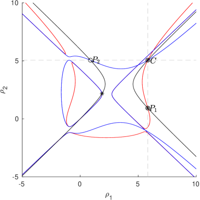
Figure 2: Intersections of the curves $p_{1}=0$ (red), $p_{2}=0$ (blue), $q=0$ (black) in the $\rho_{1}\rho_{2}$ plane.

Then we computed the rms of the preliminary orbits in Table 2 with respect to a pure Keplerian motion and selected the first orbit as the best (the one with the least rms). We propagated this orbit at the mean epoch of the observations, which is $\bar{t}=56139.99213$, applied differential corrections and computed a least squares orbit. This orbit is shown in Table 3, together with the known orbit at the same epoch.

	$a$ (au)	$e$	$I$	$\Omega$	$\omega$	$\ell$
LS	3.01802	0.05755	11.32849	104.37041	146.76038	66.54688
known	3.00997	0.05614	11.30734	104.41991	144.01204	69.25283

Table 3: Orbital elements of the least squares solution (LS) and of the known orbit. The angles $I,\Omega,\omega,\ell$ are given in degrees.

4 Joining three TSAs

Given three TSAs with attributables ${\cal A}_{1},{\cal A}_{2},{\cal A}_{3}$ at mean epochs $\bar{t}_{1},\bar{t}_{2},\bar{t}_{3}$, setting the conservation of angular momentum is enough to obtain a finite number of orbits. We review the following result, presented in [5]. Here the subscripts in ${\bf c}_{i},\rho_{i},\dot{\rho}_{i},{\bf D}_{i},{\bf E}_{i},{\bf F}_{i},{\bf G}_{i}$ refer to the three epochs.

Proposition 1.

Assume

$${\bf D}_{1}\times{\bf D}_{2}\cdot{\bf D}_{3}\neq 0.$$ (47)

Then the polynomial system

$$({\bf c}_{1}-{\bf c}_{2})\cdot{\bf D}_{1}\times{\bf D}_{2} = 0,$$ (48a)

$$({\bf c}_{1}-{\bf c}_{2})\cdot{\bf D}_{1}\times({\bf D}_{1}\times{\bf D}_{2}) = 0,$$ (48b)

$$({\bf c}_{2}-{\bf c}_{3})\cdot{\bf D}_{2}\times{\bf D}_{3} = 0,$$ (48c)

$$({\bf c}_{2}-{\bf c}_{3})\cdot{\bf D}_{2}\times({\bf D}_{2}\times{\bf D}_{3}) = 0,$$ (48d)

$$({\bf c}_{3}-{\bf c}_{1})\cdot{\bf D}_{3}\times{\bf D}_{1} = 0,$$ (48e)

$$({\bf c}_{3}-{\bf c}_{1})\cdot{\bf D}_{3}\times({\bf D}_{3}\times{\bf D}_{1}) = 0$$ (48f)

in the 6 unknowns

$$\rho_{1},\dot{\rho}_{1},\rho_{2},\dot{\rho}_{2},\rho_{3},\dot{\rho}_{3}$$

is equivalent to the redundant system

$${\bf c}_{1}={\bf c}_{2},\qquad{\bf c}_{2}={\bf c}_{3},\qquad{\bf c}_{3}={\bf c}_{1}.$$ (49)

Proof.

System (49) trivially implies (48). Assume now that system (48) holds. Using relations (48e), (48f), to prove that ${\bf c}_{3}={\bf c}_{1}$ we only need to show that

$$({\bf c}_{3}-{\bf c}_{1})\cdot{\bf v}=0$$ (50)

for some vector ${\bf v}$ that does not belong to the linear space generated by ${\bf D}_{3}\times{\bf D}_{1}$ and ${\bf D}_{3}\times({\bf D}_{3}\times{\bf D}_{1})$. Indeed we show that we can choose

$${\bf v}={\bf D}_{1}\times{\bf D}_{2}.$$

Note that

$$({\bf D}_{1}\times{\bf D}_{2})\cdot({\bf D}_{2}\times{\bf D}_{3})\times\bigl{(}{\bf D}_{2}\times({\bf D}_{2}\times{\bf D}_{3})\bigr{)}=0,$$

that is, the vector ${\bf D}_{1}\times{\bf D}_{2}$ belongs to the linear space generated by ${\bf D}_{2}\times{\bf D}_{3}$ and ${\bf D}_{2}\times({\bf D}_{2}\times{\bf D}_{3})$. Moreover, ${\bf D}_{1}\times{\bf D}_{2}$ is not generated by ${\bf D}_{3}\times{\bf D}_{1}$ and ${\bf D}_{3}\times({\bf D}_{3}\times{\bf D}_{1})$, in fact by (47) we have

$$({\bf D}_{1}\times{\bf D}_{2})\cdot({\bf D}_{3}\times{\bf D}_{1})\times\bigl{(}{\bf D}_{3}\times({\bf D}_{3}\times{\bf D}_{1})\bigr{)}=|{\bf D}_{3}\times{\bf D}_{1}|^{2}{\bf D}_{1}\times{\bf D}_{2}\cdot{\bf D}_{3}\neq 0.$$

Setting

$${\bf v}={\bf D}_{1}\times{\bf D}_{2},$$

from (48a), (48c), (48d) we obtain $({\bf c}_{1}-{\bf c}_{2})\cdot{\bf v}=({\bf c}_{2}-{\bf c}_{3})\cdot{\bf v}=0$, which yield (50) and therefore we obtain ${\bf c}_{3}={\bf c}_{1}$. In a similar way we can prove that ${\bf c}_{1}={\bf c}_{2}$, ${\bf c}_{2}={\bf c}_{3}$, provided that system (48) holds.

$\square$

∎

Equations (49) can be written as

$${\bf D}_{1}\dot{\rho}_{1}-{\bf D}_{2}\dot{\rho}_{2}={\bf J}_{12}(\rho_{1},\rho_{2}),\hskip 14.22636pt$$

$${\bf D}_{2}\dot{\rho}_{2}-{\bf D}_{3}\dot{\rho}_{3}={\bf J}_{23}(\rho_{2},\rho_{3}),\hskip 14.22636pt$$

$${\bf D}_{3}\dot{\rho}_{3}-{\bf D}_{1}\dot{\rho}_{1}={\bf J}_{31}(\rho_{3},\rho_{1}),$$

where

$${\bf J}_{12}(\rho_{1},\rho_{2}) = {\bf E}_{2}\rho_{2}^{2}-{\bf E}_{1}\rho_{1}^{2}+{\bf F}_{2}\rho_{2}-{\bf F}_{1}\rho_{1}+{\bf G}_{2}-{\bf G}_{1},$$

$${\bf J}_{23}(\rho_{2},\rho_{3}) = {\bf E}_{3}\rho_{3}^{2}-{\bf E}_{2}\rho_{2}^{2}+{\bf F}_{3}\rho_{3}-{\bf F}_{2}\rho_{2}+{\bf G}_{3}-{\bf G}_{2},$$

$${\bf J}_{31}(\rho_{3},\rho_{1}) = {\bf E}_{1}\rho_{1}^{2}-{\bf E}_{3}\rho_{3}^{2}+{\bf F}_{1}\rho_{1}-{\bf F}_{3}\rho_{3}+{\bf G}_{1}-{\bf G}_{3}.$$

Equations (48a), (48c), (48e) depend only on the radial distances. In fact, they correspond to the system

$${{\bf J}_{12}\cdot{\bf D}_{1}\times{\bf D}_{2}=0,\quad{\bf J}_{23}\cdot{\bf D}_{2}\times{\bf D}_{3}=0,\quad{\bf J}_{31}\cdot{\bf D}_{3}\times{\bf D}_{1}=0,}$$ (51)

which can be written as

$$q_{3} = a_{3}\rho_{2}^{2}+b_{3}\rho_{1}^{2}+c_{3}\rho_{2}+d_{3}\rho_{1}+e_{3}=0,$$ (52)

$$q_{1} = a_{1}\rho_{3}^{2}+b_{1}\rho_{2}^{2}+c_{1}\rho_{3}+d_{1}\rho_{2}+e_{1}=0,$$ (53)

$$q_{2} = a_{2}\rho_{1}^{2}+b_{2}\rho_{3}^{2}+c_{2}\rho_{1}+d_{2}\rho_{3}+e_{2}=0,$$ (54)

where

$$a_{3}={\bf E}_{2}\cdot{\bf D}_{1}\times{\bf D}_{2},\qquad b_{3}=-{\bf E}_{1}\cdot{\bf D}_{1}\times{\bf D}_{2},$$

$$c_{3}={\bf F}_{2}\cdot{\bf D}_{1}\times{\bf D}_{2},\qquad d_{3}=-{\bf F}_{1}\cdot{\bf D}_{1}\times{\bf D}_{2},$$

$$\hskip 28.45274pte_{3}=({\bf G}_{2}-{\bf G}_{1})\cdot{\bf D}_{1}\times{\bf D}_{2},$$

and the other coefficients $a_{j},b_{j},c_{j},d_{j},e_{j}$, for $j=1,2$, have similar expressions, obtained by cycling the indexes.

To eliminate $\rho_{1},\rho_{3}$ from (51) we can first compute the resultant

$$r=\mathrm{res}(q_{3},q_{2},\rho_{1}),$$

which depends only on $\rho_{2},\rho_{3}$, and then the resultant

$$\mathfrak{q}=\mathrm{res}(r,q_{1},\rho_{3}),$$

which is a univariate polynomial of degree 8 in the variable $\rho_{2}$.

Therefore, provided that (47) holds, to get the solutions of (49) we search for the roots $\bar{\rho}_{2}$ of $\mathfrak{q}(\rho_{2})$, compute the corresponding values $\bar{\rho}_{3}$ of $\rho_{3}$ from $r(\rho_{3},\bar{\rho}_{2})=q_{1}(\rho_{3},\bar{\rho}_{2})=0$, and the values of $\rho_{1}$ from $q_{3}(\rho_{1},\bar{\rho}_{2})=q_{2}(\bar{\rho}_{3},\rho_{1})=0.$

From equations (48b), (48d), (48f) we can write the radial velocities $\dot{\rho}_{j}$ as functions of pairs of radial distances:

$$\dot{\rho}_{2} = \frac{{\bf J}_{12}(\rho_{1},\rho_{2})\cdot{\bf D}_{1}\times({\bf D}_{1}\times{\bf D}_{2})}{|{\bf D}_{1}\times{\bf D}_{2}|^{2}},$$

$$\dot{\rho}_{3} = \frac{{\bf J}_{23}(\rho_{2},\rho_{3})\cdot{\bf D}_{2}\times({\bf D}_{2}\times{\bf D}_{3})}{|{\bf D}_{2}\times{\bf D}_{3}|^{2}},$$

$$\dot{\rho}_{1} = \frac{{\bf J}_{31}(\rho_{3},\rho_{1})\cdot{\bf D}_{3}\times({\bf D}_{3}\times{\bf D}_{1})}{|{\bf D}_{3}\times{\bf D}_{1}|^{2}}.$$

From these data we can reconstruct the orbital elements.

4.1 Straight line solutions

A particular solution of system (49) can be obtained by searching for values of $\rho_{j},\dot{\rho}_{j}$ such that

$${{\bf c}_{j}(\rho_{j},\dot{\rho}_{j})={\bf 0},\hskip 28.45274ptj=1,2,3.}$$

Let us drop the index $j$. Relation ${\bf r}\times\dot{\bf r}={\bf 0}$ implies that there exists $\lambda\in\mathbb{R}$ such that

$${\dot{\rho}{\bf e}^{\rho}+\rho\bm{\eta}+\dot{\bf q}=\lambda(\rho{\bf e}^{\rho}+{\bf q}),}$$ (55)

with $\bm{\eta}=\dot{\alpha}\cos\delta{\bf e}^{\alpha}+\dot{\delta}{\bf e}^{\delta}$. Setting $\sigma=\dot{\rho}-\lambda\rho$ we can write (55) as

$${\sigma{\bf e}^{\rho}+\rho\bm{\eta}-\lambda{\bf q}=-\dot{\bf q}.}$$ (56)

We introduce the vector

$${{\bf u}={\bf q}-({\bf q}\cdot{\bf e}^{\rho}){\bf e}^{\rho}-\frac{1}{\eta^{2}}({\bf q}\cdot\bm{\eta})\bm{\eta},}$$

which is orthogonal to both ${\bf e}^{\rho}$ and $\bm{\eta}$, where $\eta=|\bm{\eta}|$.

Thus, we can write (56) as

$${[\sigma-\lambda({\bf q}\cdot{\bf e}^{\rho})]{\bf e}^{\rho}+\Bigl{[}\rho-\frac{\lambda}{\eta^{2}}({\bf q}\cdot\bm{\eta})\Bigr{]}\bm{\eta}-\lambda{\bf u}=-\dot{\bf q}.}$$

Since $\{{\bf e}^{\rho},\bm{\eta},{\bf u}\}$ is generically an orthogonal basis of $\mathbb{R}^{3}$, we find

$${\lambda=\frac{1}{|{\bf u}|^{2}}(\dot{\bf q}\cdot{\bf u}),\qquad\rho=\frac{1}{\eta^{2}}(\lambda{\bf q}-\dot{\bf q})\cdot\bm{\eta},\qquad\dot{\rho}=\lambda\rho+(\lambda{\bf q}-\dot{\bf q})\cdot{\bf e}^{\rho}.}$$

In particular, we obtain the value

$${\rho=\frac{1}{\eta^{2}}\Bigl{(}\frac{1}{|{\bf u}|^{2}}(\dot{\bf q}\cdot{\bf u})({\bf q}\cdot\bm{\eta})-\dot{\bf q}\cdot\bm{\eta}\Bigr{)}}$$

for the radial distance, corresponding to a solution with zero angular momentum.

4.2 Selecting the solutions

Given ${\bf A}=({\cal A}_{1},{\cal A}_{2},{\cal A}_{3})$ with covariance matrices $\Gamma_{{\cal A}_{1}},\Gamma_{{\cal A}_{2}},\Gamma_{{\cal A}_{3}}$, let

$${\bf R}={\bf R}({\bf A})=\bigl{(}{\cal R}_{1}({\bf A}),{\cal R}_{2}({\bf A}),{\cal R}_{3}({\bf A})\bigr{)},\qquad{\cal R}_{i}=(\rho_{i},\dot{\rho}_{i}),\quad i=1,2,3$$

be a solution of

$$\bm{\Phi}({\bf R};{\bf A})={\bf 0},$$ (57)

with

$$\bm{\Phi}({\bf R};{\bf A})=\left(\begin{array}[]{c}({\bf c}_{1}-{\bf c}_{2})\cdot{\bf D}_{1}\times({\bf D}_{1}\times{\bf D}_{2})\cr({\bf c}_{1}-{\bf c}_{2})\cdot{\bf D}_{1}\times{\bf D}_{2}\cr({\bf c}_{2}-{\bf c}_{3})\cdot{\bf D}_{2}\times({\bf D}_{2}\times{\bf D}_{3})\cr({\bf c}_{2}-{\bf c}_{3})\cdot{\bf D}_{2}\times{\bf D}_{3}\cr({\bf c}_{3}-{\bf c}_{1})\cdot{\bf D}_{3}\times({\bf D}_{3}\times{\bf D}_{1})\cr({\bf c}_{3}-{\bf c}_{1})\cdot{\bf D}_{3}\times{\bf D}_{1}\cr\end{array}\right).$$

If $({\cal A}_{1},{\cal R}_{1}({\cal A}))$, $({\cal A}_{2},{\cal R}_{2}({\cal A}))$, and $({\cal A}_{3},{\cal R}_{3}({\cal A}))$ give bounded orbits at epochs

$$\tilde{t}_{i}=\bar{t}_{i}-\frac{\rho_{i}({\cal A})}{c},\qquad i=1,2,3,$$

then we compute the corresponding Keplerian elements. We introduce the difference vectors

$$\bm{\Delta}_{12} = \bigl{(}a_{1}-a_{2},\omega_{1}-\omega_{2},\ell_{1}-\ell_{2}-n(a_{2})(\tilde{t}_{1}-\tilde{t}_{2})\bigr{)},$$

$$\bm{\Delta}_{32} = \bigl{(}a_{3}-a_{2},\omega_{3}-\omega_{2},\ell_{3}-\ell_{2}-n(a_{2})(\tilde{t}_{3}-\tilde{t}_{2})\bigr{)},$$

where $n(a)=\sqrt{\mu}a^{-3/2}$ is the mean motion. We consider map

$$({\cal A}_{1},{\cal A}_{2},{\cal A}_{3})={\bf A}\mapsto\bm{\Psi}({\bf A})=\left({\cal A}_{2},\mathcal{R}_{2},\bm{\Delta}_{12},\bm{\Delta}_{32}\right),$$

giving the orbit $({\cal A}_{2},\mathcal{R}_{2})$ in attributable coordinates at epoch $\tilde{t}_{2}$ together with the vectors $\bm{\Delta}_{12}$, $\bm{\Delta}_{32}$, which are not constrained by the angular momentum integrals.

We map the covariance matrix

$$\Gamma_{{\bf A}}=\left[\begin{array}[]{ccc}\Gamma_{{\cal A}_{1}}&0&0\cr 0&\Gamma_{{\cal A}_{1}}&0\cr 0&0&\Gamma_{{\cal A}_{1}}\cr\end{array}\right]$$

of ${\bf A}$ into the covariance matrix of $\bm{\Psi}({\bf A})$ by the covariance propagation rule:

$$\Gamma_{\bm{\Psi}({\bf A})}=\frac{\partial\bm{\Psi}}{\partial{\bf A}}\;\Gamma_{\bf A}\;\left[\frac{\partial\bm{\Psi}}{\partial{\bf A}}\right]^{T},$$

We can check whether the considered solution of (57) fulfills the compatibility conditions

$$\bm{\Delta}_{12}=\bm{\Delta}_{32}={\bf 0}$$

within a threshold defined by $\Gamma_{\cal A}$. More precisely, consider the marginal covariance matrix $\Gamma_{\bm{\Delta}}$ of the vector

$$\bm{\Delta}=(\bm{\Delta}_{12},\bm{\Delta}_{32}).$$

The inverse matrix $C^{\bm{\Delta}}=\Gamma^{-1}_{\bm{\Delta}}$ defines a norm $\|\cdot\|_{\star}$ allowing us to test an identification between the attributables ${\cal A}_{1},{\cal A}_{2},{\cal A}_{3}$: we check whether

$$\|\bm{\Delta}\|_{\star}^{2}=\bm{\Delta}C^{\bm{\Delta}}\bm{\Delta}^{T}\leq\chi_{max}^{2},$$ (58)

where $\chi_{max}$ is a control parameter.

4.3 Numerical test with Link3

We show an application of the Link3 algorithm using three TSAs of observations of asteroid (4628) Laplace, listed in Table 4.

$\alpha$ (rad)	$\delta$ (rad)	$t$ (MJD)
5.497381	$-$0.067942	55794.33902
5.497339	$-$0.067950	55794.35011
5.497195	$-$0.067978	55794.38807
5.497148	$-$0.067987	55794.40021
0.715965	0.542095	56226.52009
0.715918	0.542080	56226.53117
0.715867	0.542063	56226.54334
0.715816	0.542047	56226.55525
0.831317	0.390743	56358.23971
0.831350	0.390746	56358.24497
0.831383	0.390749	56358.25023
0.831416	0.390751	56358.25550

Table 4: Values of right ascension ($\alpha$) and declination ($\delta$) of asteroid (4628) Laplace collected by the Pan-STARRS1 telescope.

From these observations we computed the three attributables

$$\begin{split}&{\cal A}_{1}=(5.497266,-0.067965,-0.00379969,-0.00072536)\\ &{\cal A}_{2}=(0.715891,\phantom{-}0.542071,-0.00422693,-0.00136864)\\ &{\cal A}_{3}=(0.831367,\phantom{-}0.390747,\phantom{-}0.00622482,\phantom{-}0.00054073)\end{split}$$

at the mean epochs $\bar{t}_{1}=55794.36935$, $\bar{t}_{2}=56226.53746$, $\bar{t}_{3}=56358.24760$, given in MJD. In the attributables ${\cal A}_{j}$ the angles are given in radians and the angular rates in radians/day. After discarding the straight-line solution, the solutions with negative values of $\rho$, and the unbounded ones, we are left with the radial distance triplets

$$\begin{split}&(\rho_{1},\rho_{2},\rho_{3})=(2.1955,1.9028,2.9200)\ \mathrm{au},\\ &(\rho_{1},\rho_{2},\rho_{3})=(1.9379,1.8279,2.8870)\ \mathrm{au},\end{split}$$

leading to the triplets of preliminary orbits displayed in Table 5.

	$a$ (au)	$e$	$I$	$\Omega$	$\omega$	$\ell$	$\tilde{t}$ (MJD)
	2.86808	0.30942	12.13274	274.68641	172.31982	266.26844	55794.35667
1	2.64520	0.13981	12.13274	274.68641	258.53770	242.07553	56226.52647
	2.59619	0.03219	12.13274	274.68641	290.50786	228.16130	56358.23074
	2.64614	0.11646	11.78916	275.69255	249.45265	149.80066	55794.35816
2	2.64562	0.11562	11.78916	275.69255	248.51598	249.78277	56226.52691
	2.64427	0.11343	11.78916	275.69255	247.58320	280.66987	56358.23093

Table 5: Triplets of preliminary orbits computed with Link3. The angles $I,\Omega,\omega,\ell$ are given in degrees.

Based on the norm $\|\bm{\Delta}\|_{\star}$, we selected the second triplet. Checking the rms of these orbits with respect to a pure Keplerian motion we selected the first orbit of this triplet. We propagated this orbit at the mean epoch of the 12 observations in Table 4, which is $\bar{t}=56126.38480$, applied differential corrections and computed a least squares orbit. This orbit is shown in Table 6, toghether with the known orbit at the same epoch.

	$a$ (au)	$e$	$I$	$\Omega$	$\omega$	$\ell$
LS	2.64443	0.11729	11.79295	275.66956	248.45817	227.09536
known	2.64441	0.11730	11.79294	275.66961	248.46069	227.09295

Table 6: Orbital elements of the least squares solution (LS) and of the known orbit. The angles $I,\Omega,\omega,\ell$ are given in degrees.

5 Conclusions and future work

We reviewed two initial orbit determination methods for TSAs of optical observations employing the conservation laws of Kepler’s problem. Some algebraic properties of these algorithms have also been discussed and a simple test case has been presented for both. Being based on conservation laws, these methods are suitable to link TSAs quite far apart in time, even differing by more than one orbital period of the observed body. Moreover, these algorithms are very fast, because they are based on a polynomial formulation with low degree (9 for Link2, 8 for Link3). The sensitivity of these algorithms to astrometric errors is an important feature to be investigated: in fact it seems that some orbital elements are more sensitive to these errors. Moreover, it would be important to find efficient filters to discard a priori pairs of TSAs that are not likely to belong to the same observed object. Indeed, even if some filters have been proposed in [7], [4], a satisfactory solution to this problem is still missing. The mentioned problems are currently under investigation.

6 Acknowledgements

The author wishes to thank dr. Giulio Baù for carefully reading the manuscript, and for his useful suggestions. The author has been partially supported by the MSCA-ITN Stardust-R, Grant Agreement n. 813644 under the H2020 research and innovation program. He also acknowledges the project MIUR-PRIN 20178CJA2B “New frontiers of Celestial Mechanics: theory and applications” and the GNFM-INdAM (Gruppo Nazionale per la Fisica Matematica).

References

- [1] A. Celletti and G. Pinzari. Four classical methods for determining planetary elliptic elements: a comparison. Cel. Mech. Dyn. Ast., 93:1–52, 2005.
- [2] D. Cox, J. Little, and D. O’Shea. Ideals, Varieties, and Algorithms. Springer, 2005.
- [3] C. F. Gauss. Theoria motus corporum in sectionibus conicis solem ambientium. reprinted by Dover publications in 1963, 1809.
- [4] G. F. Gronchi, G. Baù, and S. Marò. Orbit determination with the two-body integrals. III. Cel. Mech. Dyn. Ast., 123/2:105–122, 2015.
- [5] G. F. Gronchi, G. Baù, and A. Milani. Keplerian integrals, elimination theory and identification of very short arcs in a large database of optical observations. Cel. Mech. Dyn. Ast., 127/2:211–232, 2017.
- [6] G. F. Gronchi, G. Baù, Ó. Rodríguez, R. Jedicke, and J. Moeyens. A generalization of a method by Mossotti for initial orbit determination. Cel. Mech. Dyn. Ast., 133:41, 2021.
- [7] G. F. Gronchi, L. Dimare, and A. Milani. Orbit determination with the two-body integrals. Cel. Mech. Dyn. Ast., 107/3:299–318, 2010.
- [8] G. F. Gronchi, D. Farnocchia, and L. Dimare. Orbit determination with the two-body integrals. II. Cel. Mech. Dyn. Ast., 110/3:257–270, 2011.
- [9] P. S. Laplace. Mém. Acad. R. Sci. Paris, 10:93–146, 1780.
- [10] A. Milani and G. F. Gronchi. Theory of Orbit Determination. Cambridge Univ. Press, 2010.
- [11] L. G. Taff. On initial orbit determination. The Astronomical Journal, 89(6):1426–1428, 1984.
- [12] L. G. Taff and D. L. Hall. The use of angles and angular rates. I - Initial orbit determination. Celestial Mechanics, 16:481–488, 1977.
- [13] L. G. Taff, P. M. S. Randall, and S. A. Stansfield. Angles-Only, Ground-Based, Initial Orbit Determination. technical report, Lincoln Laboratory, 1984.