WORD: A large scale dataset, benchmark and clinical applicable study for abdominal organ segmentation from CT image

Abstract

Whole abdominal organ segmentation is important in diagnosing abdomen lesions, radiotherapy, and follow-up. However, oncologists’ delineating all abdominal organs from 3D volumes is time-consuming and very expensive. Deep learning-based medical image segmentation has shown the potential to reduce manual delineation efforts, but it still requires a large-scale fine annotated dataset for training, and there is a lack of large-scale datasets covering the whole abdomen region with accurate and detailed annotations for the whole abdominal organ segmentation. In this work, we establish a new large-scale Whole abdominal ORgan Dataset (WORD) for algorithm research and clinical application development. This dataset contains 150 abdominal CT volumes (30495 slices). Each volume has 16 organs with fine pixel-level annotations and scribble-based sparse annotations, which may be the largest dataset with whole abdominal organ annotation. Several state-of-the-art segmentation methods are evaluated on this dataset. And we also invited three experienced oncologists to revise the model predictions to measure the gap between the deep learning method and oncologists. Afterwards, we investigate the inference-efficient learning on the WORD, as the high-resolution image requires large GPU memory and a long inference time in the test stage. We further evaluate the scribble-based annotation-efficient learning on this dataset, as the pixel-wise manual annotation is time-consuming and expensive. The work provided a new benchmark for the abdominal multi-organ segmentation task, and these experiments can serve as the baseline for future research and clinical application development.

Dataset	Year	Organs	Scans	NSD	AFS	WAR
BTCV [23]	2015	Spleen, Kidney (L), Kidney (R), Gallbladder, Esophagus, Liver, Stomach, Aorta, Inferior vena cava, Portal vein and splenic vein, Pancreas, Adrenal gland(L), Adrenal gland(R), Duodenum	50	50	$\surd$	$\times$
DenseVNet [14]	2018	Spleen, Kidney (R), Gallbladder, Esophagus, Liver, Stomach, Splenic vein, Pancreas and Duodenum	90	$\times$	$\surd$	$\times$
CT-ORG [41]	2020	Lung, Bones, Liver, Kidneys and Bladder	140	$\times$	$\times$	$\times$
AbdomenCT-1K [34]	2021	Spleen, Kidney, Liver and Pancreas	1112	50	$\times$	$\times$
WORD dataset (ours)	2022	Liver, Spleen, Kidney(L), Kidney(R), Stomach, Gallbladder, Esophagus, Pancreas, Duodenum, Colon, Intestine, Adrenal(L), Adrenal(R), Rectum, Bladder, Head of Femur(L) and Head of Femur(R)	170	150	$\surd$	$\surd$

Table 1: Summary of several publicly available abdominal CT datasets. NSD: New Source Data (total scans); AFS: Annotate From Scratch. WAR: with the Whole Abdominal Region. To the best of our knowledge, WORD dataset is the first whole abdominal organ dataset. We corrected the results or description by the red text.

1 Introduction

Abdominal organ segmentation is a fundamental and essential task in abdominal disease diagnosis, cancer treatment, and radiotherapy planning [45]. As accurate segmentation results can provide pieces of valuable information for the clinical diagnosis and follow-ups, like organ size, location, boundary state, the spatial relationship of multiple organs, etc. In addition, organ segmentation plays a critical role in clinical treatment, especially in radiation therapy-based cancer and oncology treatments [8]. Accurate segmentation of organs at risk can alleviate potential effects on healthy organs near cancer regions. However, in clinical practice, organ segmentation is usually manually performed by radiation oncologists or radiologists. It is time-consuming and error-prone, requiring annotators to delineate and check slice-by-slice and may take several hours per case. In addition, due to the different imaging protocols/quality, and anatomical structures, fast delineation of many organs is also a challenging task for junior oncologists [16].

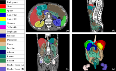
Fig. 1: An example of 16 annotated abdominal organs in a CT scan. The left table lists the annotated organs’ categories. (a), (b), (c) denote the visualization in axial, coronal, and sagittal views, respectively. (d) represents the 3D rendering results of annotated abdomen organs.

Recently, many deep learning-based methods have been proposed to accurately and quickly segment organs from abdominal CT volumes [8, 34, 52]. However, these methods were evaluated on small or in-house datasets or just segmented very few organs. In addition, previous works have also shown that some abdominal organ segmentation has achieved very promising results, such as liver, spleen, and kidney [34]. But there are still some abdominal organ segmentation tasks that are unsolved and challenging, especially for small and complex organs [34, 8]. The main reason caused these problems may be lacking a publicly available large-scale real clinical dataset with accurate whole abdominal organ annotation for research. So, developing high-quality and large-scale datasets and building benchmarks for the whole abdominal organ segmentation task is vital to boost these unsolved organ segmentation studies [34, 8].

In this work, our goal is to collect a large-scale real clinical abdomen dataset (WORD) with careful annotations. All scans in our dataset are manually segmented in great detail, covering 16 organs in the abdominal region. Due to privacy and ethical protection, collecting real clinical data is challenging and time-consuming. In addition, annotating a large-scale 3D medical image segmentation dataset is very expensive and labour-intensive, as it requires domain knowledge and clinical experience. Recently, some researchers reused previous datasets by providing annotations with pre-trained models or semi-automatic methods [34, 41], which may affect the annotator’s decision, especial regarding low-contrast boundary regions. In contrast, WORD dataset was collected from a radiation therapy center and annotated by one senior oncologist (with 7 years of experience) and then checked, discussed and refined by an experts (more than 20 years of experience). All of images were scanned before the radiotherapy treatment, without any appearance enhancement, with a similar scan location and with a similar image spacing, etc. Figure 1 shows an example from WORD.

Moreover, we investigate current methods on the WORD dataset, including fully supervised segmentation and annotation-efficient methods. Specifically, we first evaluate several state-of-the-art medical segmentation methods on the WORD, like Convolutional Neural Network-based methods nnUNet [21], Attention UNet [37], DeepLabV3+ [7], UNet++ [68] and ResUNet [10], and transformer-based approaches like CoTr [54] and UNETR [18]. After that, we investigate generalization ability of a pre-trained model on the BTCV [23] and TCIA [43]. Due to previous datasets only have annotations of few organs, we further annotate an open dataset for generalization ability evaluation, where 20 cases with the whole abdominal region were selected and annotated manually from the LiTS [1] dataset. Afterwards, we do the user study on this dataset to measure the gap between deep learning models and three oncologists. Considering these CT images have very high resolution, we investigate inference-efficient learning to reduce the memory and time cost and accelerate the inference procedure. Finally, we introduce a weakly supervised abdominal organ segmentation method with scribble annotations, which is desirable to reduce the annotation cost in the future. These attempts can be used as a new abdominal organ segmentation benchmark for further research. In summary, our contribution is two-fold:

• We build a new clinical whole abdominal organ segmentation dataset (150 CT scans) and has more categories (16 organs) and high-quality annotations than previous works [23, 14, 41, 34]. In addition, we further annotate 20 cases from LiTS [1] for networks’ generalization evaluation .

• We establish a new abdominal organ segmentation benchmark by (1) evaluating the existing fully supervised segmentation methods, (2) measuring the gap between deep learning models and oncologists, (3) investigating the pre-trained model generalization ability on open datasets, (4) investigating the inference-efficient learning for the high-resolution abdominal CT image segmentation, (5) introducing scribble-based weakly supervised methods to reduce the labeling cost.

2 Related work

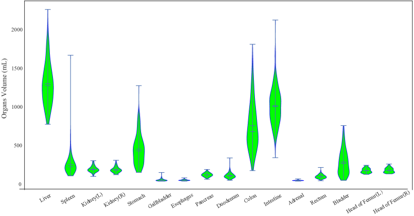
Fig. 2: Volume distribution of 16 organs in WORD.

2.1 abdominal organ segmentation datasets

Since clinical CT images of the whole abdominal region are very private and challenging to collect and annotate, few datasets with carefully annotated whole abdominal organs are publicly available. We summarize these publicly available abdominal CT datasets in Table 1. We consider the datasets with four or more annotated organs in this work. The BTCV (Beyond The Cranial Vault) [23] consists of 50 CT volumes, with 30 and 20 volumes used for training and testing, respectively. In the BTCV dataset, 13 organs are annotated manually, including the aorta, liver, spleen, right kidney, left kidney, stomach, pancreas, gallbladder, esophagus, inferior vena cava, portal vein and splenic vein, right adrenal gland, and left adrenal gland. The DenseVNet [14] has 90 CT scans, where 47 scans come from the BTCV dataset [23], and the other 43 cases come from TCIA data [43] each with annotations of eight organs. The CT-ORG [41] is an open dataset that contains 140 CT images, and five organs are annotated. Most of these images come from a challenge training set [1]. The AbdomenCT-1K dataset [34] extend five public singular organ segmentation datasets to four classes (with 1062 volumes) and a small clinical dataset (with 50 volumes coming from 20 patients). This dataset contains four organ annotations: liver, kidney, spleen, and pancreas. BTCV, DenseNet, and CT-ORG are limited by the small scale or few annotated classes to boost this topic research. Although AbdomenCT-1K is huge, the annotated organs are also too few to evaluate the efficiency of the whole abdominal segmentation task. Unlike these existing datasets, our dataset comes from a new medical center with a large scale and more annotated organs, such as the colon, intestine, rectum, etc. We believe WORD dataset is one of the most comprehensive datasets for medical image segmentation.

2.2 abdominal organ segmentation methods

Recently, deep learning-based methods have been widely used in abdominal organ segmentation tasks, especially the UNet-based deep networks [42]. The main challenge in this task lies in complex anatomical structures, the unclear boundary of soft tissues, high resolution of images, and extremely unbalanced sizes among large and small organs, etc. Many works have attempted to handle these challenges. Gibson et al. [14] proposed a DenseVNet to segment 8 organs from CT volumes, which enables high-resolution activation maps through memory-efficient dropout and feature reuse. Wang et al. [52] presented a novel framework for abdominal multi-organ segmentation using organ-attention networks with reverse connections and evaluated it on an in-house dataset. Liang et al. [25] combined the inter-and intra-patient deformation data augmentation with multi-scale Attention-UNet [44] for accurate abdominal multi-organ segmentation. Tang et al. [48] proposed a batch-based method plus random shifting strategy to boost the performance of multi-organ segmentation from high-resolution abdomen CT volumes. More recently, transformer-based methods [2, 5] are used to explicitly model the long-range dependence to capture the relationship of multi-organ for accurate segmentation.

Although the above methods have achieved promising results, they are also limited by requiring large scale carefully annotated dataset. To reduce annotation cost, Zhou et al. [67] proposed a co-training-based semi-supervised method for abdominal multi-organ segmentation, which reduces almost half of annotation cost. Furthermore, Zhou et al. [66] proposed a prior-aware neural network that incorporates anatomical priors on abdominal organ sizes to train models from several partially-labelled datasets. This work first investigates more annotation-efficient abdominal multi-organ segmentation methods with sparse annotations (scribbles). In addition, we investigate inference-efficient learning for the segmentation of high-resolution abdominal CT images to reduce the memory and time cost in the test stage.

3 WORD: Fully Annotated Clinical Whole Abdominal Organ Dataset

Characteristics	Train (n=100)	Validation (n=20)	Test (n=30)
Age (median)	47 (28-75)	52 (32-78)	49 (26-72)
Male	63	12	13
Female	37	8	17
Prostatic cancer	28	7	10
Cervical cancer	29	6	5
Rectal cancer	26	3	8
Others	17	4	7

Table 2: Clinical characteristics of WORD. Others include some metastatic tumours, such as bone metastasis and soft tissue metastasis.

Organs

Liver

Spleen

Kidney (L)

Kidney (R)

Stomach

Gallbladder

Esophagus

Pancreas

Duodenum

Colon

Intestine

Adrenal

Rectum

Bladder

Head of Femur (L)

Head of Femur (R)

Senior

1.73$\pm$0.03

1.34$\pm$0.12

1.28$\pm$0.09

1.36$\pm$0.11

3.95$\pm$0.52

6.86$\pm$1.29

7.65$\pm$2.24

7.49$\pm$2.39

9.67$\pm$4.11

4.74$\pm$2.35

3.66$\pm$1.26

9.86$\pm$4.38

3.76$\pm$1.44

2.73$\pm$0.89

1.78$\pm$0.94

1.63$\pm$0.46

Expert

0.89$\pm$0.01

0.93$\pm$0.03

1.03$\pm$0.08

0.97.$\pm$0.07

1.48$\pm$0.35

2.97$\pm$0.94

3.32$\pm$1.25

2.89$\pm$0.91

3.33$\pm$1.23

1.27$\pm$0.23

1.48$\pm$0.69

3.75$\pm$1.73

1.46$\pm$0.74

1.35$\pm$0.39

0.96$\pm$0.13

0.87$\pm$0.09

Table 3: Quantitative analysis of the inconsistent ratio ($DSC~{}(\%)$) between the annotation of senior oncologist, the expert and their consensus annotations.

3.1 Dataset summary

The 150 CT scans in the WORD dataset were collected from 150 patients before the radiation therapy in a single center. All of them are scanned by a SIEMENS CT scanner without appearance enhancement. The clinical characteristics of the WORD dataset are listed in Table 2. Each CT volume consists of 159 to 330 slices of 512 $\times$ 512 pixels, with an in-plane resolution of 0.976 mm $\times$ 0.976 mm and slice spacing of 2.5 mm to 3.0 mm, indicating that the WORD dataset is a very high-resolution dataset. All scans of WORD dataset are exhaustively annotated with 16 anatomical organs, including the liver, spleen, kidney (L), kidney (R), stomach, gallbladder, esophagus, duodenum, colon, intestine, adrenal, rectum, bladder, head of the femur (L) and head of the femur (R). An example of image and annotation from the WORD dataset is shown in Figure 1. All images were anonymized and approved by the ethics committee to protect privacy where all clinical treatment details have been deleted. We randomly split WORD dataset into three parts: 100 scans (20115 slices) for training, 20 scans (4103 slices) for validation, and 30 scans (6277 slices) for testing. Figure 2 shows the volume distributions of all annotated organs. It shows that the extremely unbalanced distribution among large and small organs may bring some challenges to the segmentation task. At the same time, we further selected and annotated 20 CT scans from LiTS [1] as an external evaluation set. These scans cover the whole abdominal region, each with 16 organ annotations.

3.2 Professional data annotation

Recently, the AbdomenCT-1K dataset [34] established an abdominal organ dataset using the pre-trained model for predictions and then refining by radiologists. At the same time, CT-ORG [41] annotated the abdominal organ by using a semi-automatic tool firstly (ITK-SNAP [62]) and then refining manually. However, these initial segmentation results could affect the annotator’s decision, especial regarding low-contrast boundary regions. Differently from AbdomenCT-1K [34] and CT-ORG [41], all scans in the WORD dataset are annotated from scratch manually. A senior oncologist (with 7 years of experience) uses ITK-SNAP [62] to delineate all organs slice-by-slice in axial view. After that, an expert in oncology (more than 20 years of experience) checks and revises these annotations carefully and discusses them in cases of disagreement to produce consensus annotations and further ensure the annotation quality. Finally, these consensus labels are released and used for methods or clinical application development and evaluation. Note that all annotations and consensus discussions obey the radiation therapy delineation guideline published by Radiation Therapy Oncology Group (RTOG). Here, we analyse the inconsistent ratio between the annotation of senior oncologist, the expert and their consensus annotations in Table 3, suggesting that annotators’ discrepancy is minor and their consensus labels are reliable. In the annotation stage, each volume roughly takes 1.2-2.6 hours to annotate all 16 organs and further requires 0.4-1.0 hours to check, discuss and refine the annotation. The WORD dataset takes us around 15 months to collect, annotate and review, so we think it’s precious and desirable to share with the medical image analysis community.

Method	nnUNet(2D)	nnUNetV2(2D)	ResUNet(2D)	DeepLabV3+(2D)	UNet++(2D)	AttUNet(3D)	nnUNet(3D)	nnUNetV2(3D)	UNETR(3D)	CoTr(3D)
Liver	95.38$\pm$4.45	96.19$\pm$2.16	96.55$\pm$0.89	96.21$\pm$1.34	96.33$\pm$1.40	96.00$\pm$1.01	96.45$\pm$0.85	96.59$\pm$6.10	94.67$\pm$1.92	95.58$\pm$1.59
Spleen	93.33$\pm$11.85	94.33$\pm$7.72	95.26$\pm$2.84	94.68$\pm$5.64	94.64$\pm$4.22	94.90$\pm$1.63	95.98$\pm$0.89	96.09$\pm$8.10	92.85$\pm$3.03	94.9$\pm$1.37
Kidney (L)	90.05$\pm$19.35	91.29$\pm$18.15	95.63$\pm$1.20	92.01$\pm$13.00	93.36$\pm$5.06	94.65$\pm$1.38	95.40$\pm$0.95	95.63$\pm$9.20	91.49$\pm$5.81	93.26$\pm$3.07
Kidney (R)	89.86$\pm$19.56	91.20$\pm$17.22	95.84$\pm$1.16	91.84$\pm$14.41	93.34$\pm$7.38	94.7$\pm$2.78	95.68$\pm$1.07	95.83$\pm$9.00	91.72$\pm$7.06	93.63$\pm$3.01
Stomach	89.97$\pm$4.96	91.12$\pm$3.60	91.58$\pm$2.86	91.16$\pm$3.07	91.33$\pm$3.13	91.15$\pm$2.74	91.69$\pm$2.5	91.57$\pm$3.05	85.56$\pm$6.12	89.99$\pm$4.49
Gallbladder	78.43$\pm$16.48	83.19$\pm$12.22	82.83$\pm$11.8	80.05$\pm$17.92	81.21$\pm$12.24	81.38$\pm$10.95	83.19$\pm$8.81	83.72$\pm$8.19	65.08$\pm$19.63	76.4$\pm$16.48
Esophagus	78.08$\pm$13.99	77.79$\pm$13.51	77.17$\pm$14.68	74.88$\pm$14.69	78.36$\pm$12.84	76.87$\pm$15.12	78.51$\pm$12.22	77.36$\pm$13.66	67.71$\pm$13.46	74.37$\pm$14.92
Pancreas	82.33$\pm$6.5	83.55$\pm$5.87	83.56$\pm$5.60	82.39$\pm$6.68	84.43$\pm$6.77	83.55$\pm$6.2	85.04$\pm$5.78	85.00$\pm$5.95	74.79$\pm$9.31	81.02$\pm$7.23
Duodenum	63.47$\pm$15.81	64.47$\pm$15.87	66.67$\pm$15.36	62.81$\pm$15.21	65.99$\pm$15.79	67.68$\pm$14.01	68.31$\pm$16.29	67.73$\pm$16.75	57.56$\pm$11.23	63.58$\pm$14.88
Colon	83.06$\pm$8.32	83.92$\pm$8.45	83.57$\pm$8.69	82.72$\pm$8.79	83.22$\pm$8.98	85.72$\pm$8.50	87.41$\pm$7.38	87.26$\pm$8.25	74.62$\pm$11.5	84.14$\pm$7.82
Intestine	85.6$\pm$4.08	86.83$\pm$4.02	86.76$\pm$3.56	85.96$\pm$4.02	86.37$\pm$4.01	88.19$\pm$3.34	89.3$\pm$2.75	89.37$\pm$3.11	80.4$\pm$4.59	86.39$\pm$3.51
Adrenal	69.9$\pm$11.07	70.0$\pm$11.86	70.9$\pm$10.12	66.82$\pm$10.81	71.04$\pm$10.65	70.23$\pm$9.31	72.38$\pm$8.98	72.98$\pm$8.09	60.76$\pm$8.32	69.06$\pm$9.26
Rectum	81.66$\pm$6.64	81.49$\pm$7.37	82.16$\pm$6.73	81.85$\pm$6.67	81.44$\pm$6.7	80.47$\pm$5.44	82.41$\pm$4.9	82.32$\pm$5.26	74.06$\pm$8.03	80.0$\pm$5.4
Bladder	90.49$\pm$14.73	90.15$\pm$16.85	91.0$\pm$13.5	90.86$\pm$14.07	92.09$\pm$11.53	89.71$\pm$15.00	92.59$\pm$8.27	92.11$\pm$9.75	85.42$\pm$18.17	89.27$\pm$18.28
Head of Femur (L)	93.28$\pm$5.31	93.28$\pm$5.12	93.39$\pm$5.11	92.01$\pm$4.76	93.38$\pm$5.12	91.90$\pm$4.39	91.99$\pm$4.72	92.56$\pm$4.19	89.47$\pm$6.4	91.03$\pm$4.81
Head of Femur (R)	93.78$\pm$4.38	93.93$\pm$4.29	93.88$\pm$4.30	92.29$\pm$4.01	93.88$\pm$4.21	92.43$\pm$3.68	92.74$\pm$3.63	92.49$\pm$4.03	90.17$\pm$4.0	91.87$\pm$3.32
Mean	84.92$\pm$5.39	85.80$\pm$5.27	86.67$\pm$4.81	84.91$\pm$5.05	86.28$\pm$3.96	86.21$\pm$4.78	87.44 $\pm$4.33	87.41$\pm$4.57	79.77$\pm$4.92	84.66$\pm$5.45

Table 4: Performance comparison ($DSC~{}(\%)$) of 16 abdominal organs segmentation using ten recent segmentation methods.

Method	nnUNet(2D)	nnUNetV2(2D)	ResUNet(2D)	DeepLabV3+(2D)	UNet++(2D)	AttUNet(3D)	nnUNet(3D)	nnUNetV2(3D)	UNETR(3D)	CoTr(3D)
Liver	7.94$\pm$17.23	7.34$\pm$16.48	4.64$\pm$7.37	6.81$\pm$18.3	11.77$\pm$22.17	3.61$\pm$1.75	3.31$\pm$1.38	3.17$\pm$0.51	8.36$\pm$14.13	7.47$\pm$12.18
Spleen	14.46$\pm$41.27	9.53$\pm$33.84	8.7$\pm$30.11	8.93$\pm$33.61	9.39$\pm$32.14	2.74$\pm$1.61	2.15$\pm$0.5	2.12$\pm$0.47	14.84$\pm$34.62	8.14$\pm$24.43
Kidney (L)	10.53$\pm$29.43	10.33$\pm$29.52	5.4$\pm$15.85	10.4$\pm$29.39	13.09$\pm$29.75	6.28$\pm$19.19	6.07$\pm$19.38	2.46$\pm$0.7	23.37$\pm$39.28	16.42$\pm$27.79
Kidney (R)	10.73$\pm$28.49	10.85$\pm$28.41	2.47$\pm$0.97	10.02$\pm$28.0	21.84$\pm$42.61	2.86$\pm$1.46	2.35$\pm$0.81	2.24$\pm$0.47	7.9$\pm$19.08	12.79$\pm$29.76
Stomach	19.04$\pm$20.82	13.97$\pm$12.08	9.98$\pm$6.62	11.01$\pm$8.45	15.4$\pm$21.44	8.23$\pm$6.07	8.47$\pm$5.96	9.47$\pm$7.61	19.25$\pm$23.19	10.26$\pm$9.49
Gallbladder	8.9$\pm$10.33	7.91$\pm$8.67	9.48$\pm$12.97	7.36$\pm$9.43	14.68$\pm$28.48	5.11$\pm$3.41	5.24$\pm$5.3	6.04$\pm$5.63	12.72$\pm$15.39	11.32$\pm$15.57
Esophagus	6.9$\pm$9.72	6.7$\pm$7.8	6.7$\pm$7.6	7.6$\pm$8.45	5.85$\pm$3.93	5.35$\pm$3.79	5.49$\pm$4.34	5.83$\pm$4.64	9.31$\pm$8.41	6.29$\pm$4.53
Pancreas	7.92$\pm$7.34	7.82$\pm$6.76	7.82$\pm$7.15	7.67$\pm$7.1	7.5$\pm$8.45	6.96$\pm$7.39	6.84$\pm$7.9	6.87$\pm$7.86	10.66$\pm$8.56	8.88$\pm$10.61
Duodenum	25.18$\pm$18.39	23.29$\pm$14.39	21.79$\pm$12.83	21.61$\pm$13.88	23.67$\pm$13.8	21.61$\pm$12.86	21.3$\pm$14.22	21.15$\pm$14.26	25.15$\pm$21.96	24.83$\pm$15.47
Colon	15.56$\pm$12.97	15.68$\pm$14.0	17.41$\pm$15.22	15.95$\pm$14.07	16.97$\pm$13.92	10.21$\pm$12.87	9.99$\pm$13.17	10.42$\pm$14.27	20.32$\pm$14.37	12.41$\pm$12.75
Intestine	10.46$\pm$6.24	8.96$\pm$4.83	9.54$\pm$7.2	9.57$\pm$5.21	10.06$\pm$6.01	5.68$\pm$3.93	5.14$\pm$3.68	5.27$\pm$4.29	12.62$\pm$7.63	7.96$\pm$5.58
Adrenal	6.06$\pm$3.99	6.42$\pm$4.3	6.67$\pm$4.59	7.14$\pm$4.8	7.14$\pm$4.97	5.98$\pm$4.01	5.46$\pm$4.04	5.43$\pm$3.82	8.73$\pm$5.3	6.76$\pm$6.99
Rectum	10.62$\pm$5.5	11.15$\pm$7.33	10.62$\pm$6.52	10.96$\pm$6.94	11.54$\pm$8.13	11.67$\pm$6.37	11.57$\pm$6.95	12.39$\pm$8.12	12.79$\pm$6.38	11.26$\pm$6.06
Bladder	5.88$\pm$7.21	4.97$\pm$5.26	5.02$\pm$6.17	5.14$\pm$6.22	5.06$\pm$6.56	4.83$\pm$4.66	3.68$\pm$2.23	4.17$\pm$3.6	14.71$\pm$40.82	14.34$\pm$43.85
Head of Femur (L)	6.56$\pm$8.09	6.54$\pm$8.13	6.56$\pm$8.3	7.62$\pm$7.93	6.66$\pm$8.22	6.93$\pm$6.27	35.18$\pm$88.78	17.05$\pm$62.15	38.11$\pm$98.44	19.42$\pm$70.83
Head of Femur (R)	5.89$\pm$7.55	5.74$\pm$6.76	5.98$\pm$7.2	7.02$\pm$6.76	16.92$\pm$63.02	6.06$\pm$4.78	33.03$\pm$82.19	27.29$\pm$81.62	38.62$\pm$99.75	26.78$\pm$78.4
Mean	10.79$\pm$10.29	9.88$\pm$9.16	8.6$\pm$6.47	9.67$\pm$9.06	12.35$\pm$15.87	7.13$\pm$4.68	10.33$\pm$26.65	8.84$\pm$ 22.63	17.34$\pm$28.8	12.83$\pm$21.96

Table 5: Performance comparison ($HD_{95}~{}(mm)$) of 16 abdominal organs segmentation using ten recent segmentation methods.

3.3 Potential research topics

We can conduct many essential research topics on medical image segmentation/detection methods and clinical application with the large and carefully annotated abdominal multi-organ dataset. Besides, there are some challenges in the WORD, including the imbalanced sample among large and small size organs, the high resolution, and the complex anatomical structure. It can be used to develop or evaluate clinical application, as it is very desirable to develop a tool or software to assist oncologists in delineating organs quickly and accurately. The WORD dataset also can be employed in general algorithm research, such as fully-/semi-/weakly-supervised learning, domain adaption/generalization, partially label and lifelong learning, etc. Here, we roughly summarized the potential research topics as follows.

3.3.1 Fully-supervised abdominal organ segmentation and generalization

Fully supervised learning [21] aims to efficiently utilize the labelled data to achieve good results and solve the challenges of imbalanced distributions and complex structures. It is a fundamental topic and has been studied for many years. Here, we presented a new abdominal organ segmentation dataset to boost abdominal organ segmentation algorithm research, evaluation, and comparison. Afterwards, we further build a publicly external evaluation dataset from LiTS [1] for segmentation models’ generalization evaluation. In addition, the WORD dataset and the external dataset can be used to develop clinical application or clinically applicable evaluations.

3.3.2 Abdominal organ segmentation with low computational cost and high speed

For 3D abdominal CT scans, the inference stage always takes much time and GPU memory due to the high dimension and resolution. To deal with this issue, inference-efficient model [13] is proposed to achieve the trade-off between high-performance and low inference cost. However, very few works have been studied to accelerate the inference of 3D medical image segmentation tasks [48]. Recently, knowledge distillation has achieved success in several 2D natural image recognition tasks, which may have the potential to handle the 3D medical image segmentation tasks [35].

3.3.3 Abdominal organ segmentation with low annotation cost

Pixel-wise abdominal organ annotation is very expensive, requiring clinical experience and much time. Recently, annotation-efficient learning [28, 67, 30, 32] has been introduced to reduce the labeling cost and improve the network generalization ability by semi-/weakly-supervised learning, domain adaptation strategies, etc. These strategies have been scorching topics and show the potential to reduce annotation cost by utilizing unlabeled data or sparse annotations. Reducing the annotation cost for accurate abdominal organ segmentation is desirable, as it can accelerate the model development and reduce cost. In this work, we pay more attention to evaluating weakly supervised methods to reduce labeling cost.

4 Experiments and Analyses

4.1 Implementations and metrics

In this work, all methods are implemented, trained, and tested by PyTorch 1.8 [39] on a cluster with eight NVIDIA GTX1080TI GPUs. We choose the powerful nnUNet [21] as our baseline for fair comparisons. nnUNet is a self-configuration segmentation framework without needing any manual effort for data processing, training planning (network architectures and parameters setting, etc.), and post-processing, and has won more than 19 medical segmentation challenges [21]. Due to that the nnUNet just provides implementation of the vanilla UNet network, we further adapt it to support more network architectures. Note that we use the public implementations of the compared methods. We employ the default settings of nnUNet as our experimental settings, where the batch size is 2 for 3D methods and 12 for 2D methods, the total epoch is 1000, and the loss function is a combination of cross-entropy and dice loss. All the models are trained and tested based on the default settings, except that we don’t use the test time augmentation, as each model needs more than six GPU days to train, and each volume takes more than five minutes to infer. We use two widely-used metrics to measure the segmentation quality in this work: 1) Dice similarity coefficient ($DSC$) is used to evaluate the pixel-wise overlap between the ground truth and prediction; 2) 95% Hausdorff Distance ($HD_{95}$) that measures distance difference between the boundaries of the ground truth and prediction. The implementations of $DSC$ and $HD_{95}$ are available.

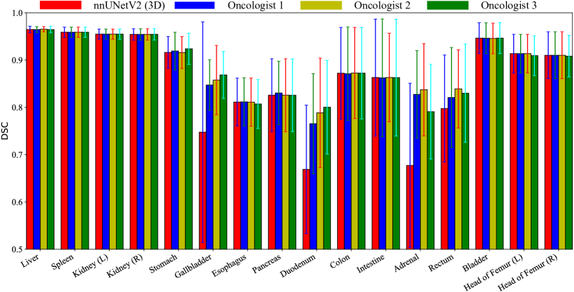
Fig. 3: User study based on three junior oncologists independently, each of them comes from a different hospital.

4.2 Fully-supervised abdominal organ segmentation

We first evaluate some existing state-of-the-art (SOTA) methods on the WORD dataset. Then, we further evaluate the gap between the deep network and three oncologists. Finally, we investigate the domain shift between the WORD dataset and three public datasets (BTCV [23], TCIA [43], and LiTS [1]).

4.2.1 Evaluations of SOTA methods on the WORD

For deep learning-based clinical application, fully supervised learning is one of the most basic and popular solutions, especially in automatic multi-organ delineation systems. In this work, we investigate several existing SOTA methods on the WORD dataset, including convolutional neural networks-based networks, nnUNet [21] and its variations (both 2D and 3D), ResUNet [10], DeepLabV3+ [7], UNet++ [68] and Attention-UNet (AttUNet) [37], and transformer-based architectures, CoTr [54] and UNETR [18]. The quantitative segmentation results in term of $DSC$ and $HD_{95}$ are presented in Table 4 and Table 5, respectively. It can be observed that all CNN-based methods outperform transformer-based CoTr [54] and UNETR [18]. Moreover, the results further show that all SOTA methods can achieve very promising results ($DSC$ $\textgreater$ 85%) on large organs, such as the liver, spleen, kidney, stomach, bladder, and head of the femur. It has also proven that the large organ segmentation task is a well-solved problem if there are enough high-quality annotated samples. But for the gallbladder, pancreas, and rectum segmentation, almost all methods get poor results, where $DSC$ $\textless$ 85% and $HD_{95}$ $\textgreater$ 10$mm$. In addition, the the segmentation results of esophagus, duodenum and adrenal are extremely bad, where almost all methods achieve $DSC$ $\textless$ 70%. All the above results show that the segmentation of small organs remains challenging and needs more attention to be paid. However, few works and researchers have focused on solving these challenging tasks. One of the critical reasons is lacking large-scale and publicly available datasets and benchmarks. To alleviate these challenges, we build the WORD dataset and corresponding benchmarks to boost research in the medical image computing community.

4.2.2 User study by three oncologists

Then, we employ a comprehensive user study to measure the gap between the network and three oncologists. Following the general workflow of deep learning-assisted organs delineation systems [8], we invite three junior oncologists (with 3 years of experience) from three different hospitals to revise model-generated predictions independently until the results are clinically acceptable. We randomly selected 20 predictions produced by nnUNetV2 (3D) for the user study and calculated the revised results. The quantitative comparison in terms of $DSC$ between the nnUNet predictions and three oncologists’ revised results are presented in Figure 3. For organs with large size and clear boundary, the deep network can produce promising results that are very close to clinically applicable with just a few revisions. However, there is a massive gap between the deep network and junior oncologists in small organ segmentation. It indicates that the deep network has the potential to reduce the burden of oncologists in annotating large organs. In the future, combining the user interaction with the deep network may help further to reduce the burden of delineating small organs and accelerate the clinical workflow [33, 51].

DataSet	TCIA		BTCV		LiTS
Method	nnUNetV2 (2D)	nnUNetV2 (3D)	nnUNetV2 (2D)	nnUNetV2 (3D)	nnUNetV2 (2D)	nnUNetV2 (3D)
Liver	91.27$\pm$3.71	92.59$\pm$3.72	86.63$\pm$7.79	93.36$\pm$5.75	92.37$\pm$3.48	94.2$\pm$1.41
Spleen	85.47$\pm$13.97	86.31$\pm$12.57	72.43$\pm$19.36	88.89$\pm$11.78	84.73$\pm$14.43	95.28$\pm$5.44
Kidney (L)	80.24$\pm$13.4	91.44$\pm$5.13	64.57$\pm$23.94	87.36$\pm$16.25	79.23$\pm$19.24	96.33$\pm$3.83
Kidney (R)	-	-	37.32$\pm$33.71	56.22$\pm$42.99	78.51$\pm$22.39	96.07$\pm$4.84
Stomach	54.32$\pm$21.73	73.37$\pm$17.35	51.73$\pm$22.74	78.52$\pm$18.54	68.46$\pm$15.88	86.43$\pm$13.68
Gallbladder	54.0$\pm$32.36	78.49$\pm$18.33	40.38$\pm$32.44	63.82$\pm$32.05	49.05$\pm$32.97	60.15$\pm$34.37
Esophagus	54.62$\pm$21.38	61.22$\pm$18.85	47.1$\pm$18.37	62.53$\pm$15.28	84.77$\pm$5.04	87.13$\pm$6.8
Pancreas	51.38$\pm$21.59	68.53$\pm$15.25	49.64$\pm$17.59	73.64$\pm$13.15	59.59$\pm$12.78	89.43$\pm$4.16
Duodenum	33.15$\pm$18.92	51.14$\pm$15.78	24.19$\pm$14.78	56.19$\pm$15.62	45.01$\pm$15.52	76.45$\pm$6.4
Colon	-	-	-	-	75.42$\pm$14.65	87.54$\pm$8.32
Intestine	-	-	-	-	64.35$\pm$10.77	83.6$\pm$6.87
Adrenal	-	-	17.01$\pm$20.72	41.72$\pm$32.5	62.86$\pm$14.16	85.89$\pm$4.49
Rectum	-	-	-	-	68.93$\pm$24.83	80.61$\pm$19.57
Bladder	-	-	-	-	91.63$\pm$5.94	92.88$\pm$7.43
Head of Femur (L)	-	-	-	-	93.26$\pm$2.37	95.55$\pm$2.63
Head of Femur (R)	-	-	-	-	92.73$\pm$3.12	94.98$\pm$3.51
Mean	63.06$\pm$7.79	75.39$\pm$5.50	49.10$\pm$7.34	70.23$\pm$10.97	74.43$\pm$8.29	87.66$\pm$7.98

Table 6: The segmentation result ($DSC~{}(\%)$) of the BTCV [23], TCIA [43] and LiTS [1] using the pre-trained (on the WORD) nnUNetV2 (2D/3D).

DataSet	TCIA		BTCV		LiTS
Method	nnUNetV2 (2D)	nnUNetV2 (3D)	nnUNetV2 (2D)	nnUNetV2 (3D)	nnUNetV2 (2D)	nnUNetV2 (3D)
Liver	29.39$\pm$20.67	17.11$\pm$24.27	44.73$\pm$36.15	13.96$\pm$23.73	32.28$\pm$27.58	11.57$\pm$9.76
Spleen	87.32$\pm$69.61	31.11$\pm$45.85	128.28$\pm$59.62	37.46$\pm$67.09	90.59$\pm$63.72	12.13$\pm$21.25
Kidney (L)	92.93$\pm$49.56	15.44$\pm$39.47	107.0$\pm$40.9	20.34$\pm$38.08	96.44$\pm$51.64	12.15$\pm$29.13
Kidney (R)	-	-	71.58$\pm$43.5	27.8$\pm$28.6	69.78$\pm$64.44	10.16$\pm$34.59
Stomach	43.17$\pm$23.49	26.75$\pm$22.28	65.47$\pm$42.91	31.42$\pm$40.64	47.33$\pm$31.66	17.87$\pm$28.48
Gallbladder	34.94$\pm$40.91	7.65$\pm$11.62	53.34$\pm$61.11	16.69$\pm$21.8	28.22$\pm$38.44	18.63$\pm$22.57
Esophagus	17.41$\pm$9.98	15.85$\pm$9.66	22.25$\pm$15.17	18.81$\pm$18.02	4.44$\pm$2.17	5.91$\pm$8.08
Pancreas	31.37$\pm$8.59	15.59$\pm$13.67	30.15$\pm$15.12	13.12$\pm$18.01	27.21$\pm$11.79	4.93$\pm$3.66
Duodenum	34.09$\pm$14.13	35.07$\pm$18.54	50.97$\pm$26.19	29.0$\pm$15.09	25.97$\pm$9.99	15.75$\pm$9.52
Colon	-	-	-	-	31.89$\pm$14.66	24.82$\pm$45.11
Intestine	-	-	-	-	31.15$\pm$10.63	12.11$\pm$6.55
Adrenal	-	-	26.28$\pm$37.47	5.29$\pm$9.75	6.11$\pm$3.27	2.22$\pm$0.72
Rectum	-	-	-	-	44.38$\pm$111.99	10.27$\pm$9.8
Bladder	-	-	-	-	33.46$\pm$117.57	54.35$\pm$149.16
Head of Femur (L)	-	-	-	-	32.35$\pm$115.82	30.88$\pm$116.82
Head of Femur (R)	-	-	-	-	59.42$\pm$161.8	58.08$\pm$162.04
Mean	46.33$\pm$20.34	20.57$\pm$12.30	60.00$\pm$15.01	21.39$\pm$15.96	41.31$\pm$47.99	18.86$\pm$50.87

Table 7: The segmentation result ($HD_{95}~{}(mm)$) of the BTCV [23], TCIA [43] and LiTS [1] using the pre-trained (on the WORD) nnUNetV2 (2D/3D).

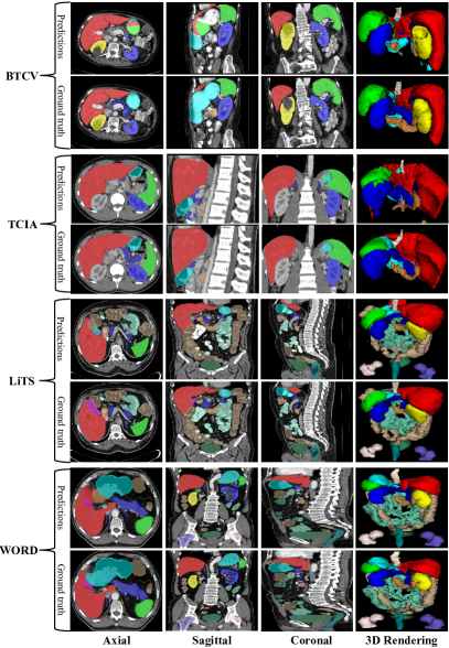
Fig. 4: Visual comparison of segmentation performance on four different datasets. All predictions were produced by the nnUNetV2 (3D) pre-trained on the WORD.

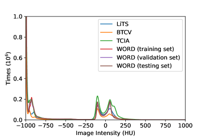
Fig. 5: Intensity distributions comparison of LiTS, BTCV, TCIA and WORDs. HU means Hounsfield Unit.

4.2.3 Generalization on BTCV, TCIA and LiTS

We further investigate the domain shift between the WORD dataset and three widely-used public datasets BTCV [23], TCIA [43] and LiTS [1]. The differences between the WORD dataset and BTCV [23], TCIA [43] and LiTS [1] lie in 1) coming from different centres/scanners/countries; 2) suffering from different diseases; 3) with different phase/contrast enhancement; 4) with different voxel spacing; 5) annotating by different oncologists/radiologists. All of them could affect the generalizability of the deep network and further limit clinical practice. In this work, we use the pre-trained model on the WORD dataset to infer the samples from BTCV [23] (47 scans), TCIA [43] (43 scans) and LiTS [1] (20 scans) to estimate the domain gap. Table 6 and Table 7 list the results of $DSC$ and $HD_{95}$, respectively. Here, we just consider the official annotated organs of the BTCV [23] and TCIA [43] datasets. It can be found that there are very significant domain shifts between WORD dataset and BTCV [23], TCIA [43] datasets, as the pre-trained nnUNet on the WORD dataset performs very worse on the BTCV [23] and TCIA [43]. For the LiTS [1] dataset, the nnUNetV2(3D) achieves very encouraging results, even better than the results of WORD. But the nnUNetV2(2D) still performs badly, which may be caused by that the nnUNetV2(2D) did not consider the relationship between neighbouring slices. It also indicates that the model generalization for the multi-site abdominal organ task is not a solved problem. Figure 4 shows some segmentation results of different datasets. These results are generated by a pre-trained nnUNetV2(3D) on the WORD. It can be observed that the results of TCIA and BTCV are inaccurate, which indicates that there is a significant domain gap between TCIA/BTCV and WORD. In contrast, the result of LiTS is better and more promising; the reason may be the domain gap between LiTS and WORD dataset is minor. In addition, we further analyse the intensity distributions between LiTS [1], BTCV [23], TCIA [43], and WORD in Figure 5. It shows there are bigger intensity distribution gaps between WORD dataset and BTCV/TCIA than LiTS, which conforms to segmentation results.

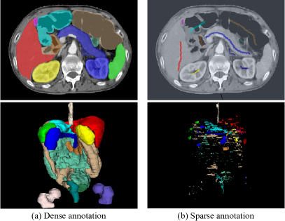
Fig. 6: Different types of medical image annotation, the first and second rows show the visualization in 2D and 3D spaces, respectively.

Method	nnUNetV2(3D)	ESPNet	ESPNet+KD	DMFNet	DMFNet+KD	LCOVNet	LCOVNet+KD
Liver	96.59$\pm$6.10	76.47$\pm$19.12	95.64$\pm$0.9	95.8$\pm$0.79	95.96$\pm$0.76	95.37$\pm$1.2	95.89$\pm$0.58
Spleen	96.09$\pm$8.10	84.54$\pm$19.81	93.9$\pm$3.22	94.25$\pm$2.15	94.64$\pm$2.53	94.6$\pm$2.08	95.4$\pm$2.14
Kidney (L)	95.63$\pm$9.20	85.23$\pm$20.96	92.24$\pm$6.04	94.72$\pm$0.97	94.7$\pm$1.01	94.78$\pm$1.18	95.17$\pm$1.13
Kidney (R)	95.83$\pm$9.00	89.65$\pm$15.74	94.39$\pm$1.61	95.0$\pm$1.12	94.96$\pm$1.19	95.08$\pm$1.14	95.78$\pm$0.84
Stomach	91.57$\pm$3.05	82.87$\pm$12.06	87.37$\pm$7.26	89.69$\pm$3.43	89.88$\pm$5.24	90.06$\pm$3.32	90.86$\pm$3.82
Gallbladder	83.72$\pm$8.19	49.02$\pm$29.45	67.19$\pm$24.84	77.12$\pm$17.7	79.84$\pm$11.81	75.48$\pm$13.46	78.87$\pm$11.8
Esophagus	77.36$\pm$13.66	59.46$\pm$23.21	67.91$\pm$14.27	74.41$\pm$12.08	74.1$\pm$14.81	76.51$\pm$11.87	74.55$\pm$13.55
Pancreas	85.00$\pm$5.95	56.35$\pm$21.93	75.78$\pm$8.68	81.9$\pm$6.88	81.66$\pm$7.12	81.46$\pm$9.11	82.59$\pm$7.54
Duodenum	67.73$\pm$16.75	38.39$\pm$22.04	62.03$\pm$15.85	63.96$\pm$16.44	66.66$\pm$16.18	66.55$\pm$16.02	68.23$\pm$15.04
Colon	87.26$\pm$8.25	71.54$\pm$12.12	78.77$\pm$10.61	83.77$\pm$8.45	83.51$\pm$7.68	85.61$\pm$7.19	84.22$\pm$7.32
Intestine	89.37$\pm$3.11	72.44$\pm$8.26	72.8$\pm$8.62	86.38$\pm$3.77	86.95$\pm$3.11	87.36$\pm$3.55	87.19$\pm$3.06
Adrenal	72.98$\pm$8.09	25.41$\pm$20.05	60.55$\pm$11.13	68.26$\pm$7.83	66.73$\pm$8.13	70.08$\pm$8.67	69.82$\pm$8.54
Rectum	82.32$\pm$5.26	72.48$\pm$9.86	74.32$\pm$15.16	79.24$\pm$7.09	79.26$\pm$8.57	80.64$\pm$7.21	79.99$\pm$6.82
Bladder	92.11$\pm$9.75	89.83$\pm$8.59	78.58$\pm$29.82	87.54$\pm$17.11	88.18$\pm$15.91	87.6$\pm$15.88	88.18$\pm$17.64
Head of Femur (L)	92.56$\pm$4.19	84.32$\pm$4.98	88.24$\pm$2.81	91.71$\pm$4.44	91.99$\pm$4.61	91.74$\pm$4.36	92.48$\pm$3.75
Head of Femur (R)	92.49$\pm$4.03	89.12$\pm$2.69	89.04$\pm$2.42	92.04$\pm$3.22	92.55$\pm$3.93	92.0$\pm$3.58	93.23$\pm$3.46
Mean	87.41$\pm$4.57	70.45$\pm$7.29	79.92$\pm$8.01	84.74$\pm$5.65	85.1$\pm$5.09	85.31$\pm$5.02	85.82$\pm$4.89

Table 8: Quantitative comparison between various efficient segmentation methods in term of $DSC~{}(\%)$. The teacher network is the well-trained nnUNetV2(3D). We corrected the results or description by the red text.

Method	nnUNetV2(3D)	ESPNet	ESPNet+KD	DMFNet	DMFNet+KD	LCOVNet	LCOVNet+KD
Liver	3.17$\pm$0.51	22.33$\pm$16.56	3.89$\pm$1.12	3.79$\pm$0.96	3.45$\pm$0.84	15.25$\pm$52.03	5.52$\pm$6.11
Spleen	2.12$\pm$0.47	8.98$\pm$11.86	14.35$\pm$37.18	4.11$\pm$5.55	4.63$\pm$7.24	3.64$\pm$3.95	4.32$\pm$7.09
Kidney (L)	2.46$\pm$0.7	9.94$\pm$15.51	4.52$\pm$4.65	2.79$\pm$0.52	2.91$\pm$0.64	2.81$\pm$0.74	3.19$\pm$0.83
Kidney (R)	2.24$\pm$0.47	5.06$\pm$6.34	2.87$\pm$0.91	2.64$\pm$0.49	2.61$\pm$0.48	2.56$\pm$0.45	2.81$\pm$0.52
Stomach	9.47$\pm$7.61	16.8$\pm$14.66	19.0$\pm$24.07	9.41$\pm$5.5	10.83$\pm$9.36	9.1$\pm$5.49	15.97$\pm$32.96
Gallbladder	6.04$\pm$5.63	20.37$\pm$18.03	12.26$\pm$13.69	6.57$\pm$8.71	6.21$\pm$6.91	6.42$\pm$4.86	11.86$\pm$26.18
Esophagus	5.83$\pm$4.64	15.49$\pm$14.52	10.5$\pm$10.36	6.39$\pm$4.83	6.17$\pm$4.37	5.97$\pm$3.23	7.09$\pm$8.06
Pancreas	6.87$\pm$7.86	25.18$\pm$22.03	11.49$\pm$9.72	8.02$\pm$8.38	8.23$\pm$8.84	9.91$\pm$13.95	8.4$\pm$10.69
Duodenum	21.15$\pm$14.26	41.61$\pm$19.34	32.64$\pm$30.05	23.28$\pm$14.73	20.32$\pm$13.11	20.65$\pm$13.35	19.4$\pm$11.39
Colon	10.42$\pm$14.27	73.68$\pm$83.07	20.68$\pm$13.62	11.18$\pm$11.71	11.11$\pm$12.13	9.55$\pm$11.72	12.51$\pm$13.22
Intestine	5.27$\pm$4.29	17.47$\pm$8.02	17.64$\pm$7.75	6.85$\pm$4.34	6.59$\pm$4.02	6.04$\pm$3.6	6.82$\pm$3.86
Adrenal	5.43$\pm$3.82	32.45$\pm$21.58	10.45$\pm$11.4	6.3$\pm$3.24	6.75$\pm$4.41	5.82$\pm$4.44	6.06$\pm$4.07
Rectum	12.39$\pm$8.12	18.35$\pm$8.25	18.87$\pm$19.96	11.41$\pm$5.51	12.48$\pm$6.14	10.16$\pm$4.55	12.07$\pm$6.68
Bladder	4.17$\pm$3.6	5.1$\pm$2.74	20.03$\pm$50.47	5.93$\pm$6.02	5.3$\pm$4.87	6.89$\pm$6.67	6.24$\pm$8.67
Head of Femur (L)	17.05$\pm$62.15	12.69$\pm$4.91	22.97$\pm$58.09	6.52$\pm$6.52	6.58$\pm$6.61	17.68$\pm$58.9	17.09$\pm$55.62
Head of Femur (R)	27.29$\pm$81.62	9.41$\pm$3.49	18.18$\pm$21.9	6.14$\pm$4.33	6.1$\pm$5.6	30.83$\pm$93.82	6.5$\pm$5.78
Mean	8.84$\pm$ 22.63	20.93$\pm$18.13	15.02$\pm$16.3	7.58$\pm$3.72	7.52$\pm$3.59	10.21$\pm$25.87	9.11$\pm$13.87

Table 9: Quantitative comparison between various efficient segmentation methods in term of $HD_{95}~{}(mm)$. The teacher network is the well trained nnUNetV2(3D).

Method

Background

Liver

Spleen

Kidney (L)

Kidney (R)

Stomach

Gallbladder

Esophagus

Pancreas

Duodenum

Colon

Intestine

Adrenal

Rectum

Bladder

Head of Femur (L)

Head of Femur (R)

Ratio (%)

0.23$\pm$0.03

1.79$\pm$0.3

2.82$\pm$0.51

1.89$\pm$0.51

1.95$\pm$0.42

1.97$\pm$0.34

7.32$\pm$3.75

9.99$\pm$3.9

4.57$\pm$2.11

5.9$\pm$3.23

1.8$\pm$0.36

1.75$\pm$0.33

19.76$\pm$4.34

2.35$\pm$1.19

1.58$\pm$1.19

1.23$\pm$0.25

1.08$\pm$0.28

Table 10: Labeling cost of scribble annotation compared with dense annotation. Here, we reported the percentage of labeled voxels between scribble and dense annotation.

4.3 Abdominal organ segmentation with low computational cost and high speed

Although large-scale deep models have achieved promising results for abdominal organ segmentation [21, 66, 48], these heavy models require various expensive computations and storage components and a long inference time [40]. In addition, the whole abdominal CT image has a very high resolution, which further increases the GPU memory budget and computational cost [40, 48]. So, it is desirable to investigate the high-performance and low computational cost method for abdominal organ segmentation, and it is also suitable for clinical scenarios. This study investigates the efficient abdominal organ segmentation topic and compares several lightweight network-based and knowledge distillation methods on the WORD. Firstly, we compare three lightweight segmentation networks’ performance in abdominal organ segmentation, ESPNet [36], DMFNet [4] and LCOVNet [65]. ESPNet [36] proposed an efficient spatial pyramid block for high-speed brain tumour segmentation. DMFNet [4] combined point-wise [64], group-wise [9] and atrous [6] convolutions to reduce the computational cost and boost brain tumour segmentation performance. LCOVNet [65] proposed an attention based spatiotemporal separable convolution for efficient COVID-19 pneumonia lesion segmentation. Afterwards, we study the knowledge distillation strategy for the efficient high-resolution image segmentation [20]. In general, knowledge distillation aims to transfer the knowledge of a heavy model (teacher) to a lightweight model (student) and encourages the student to achieve similar or comparable results to the teacher. Following the general knowledge distillation [20, 40], we used a pre-trained nnUNetV2(3D) as the teacher model and employed the logit output of nnUNetV2(3D) to guide the student models (ESPNet, DMFNet and LCOVNet). Table 8 and 9 list the quantitative results of different methods in terms of $DSC$ and $HD_{95}$. It can be observed that the knowledge distillation strategy can improve student models’ performance. In Table 12, we further analyze the model complexity of the teacher network and student networks in the same software and hardware environments . These results show that combining lightweight networks and knowledge distillation can achieve a better trade-off between performance and computational cost. This study further indicates that exploring more power lightweight networks and knowledge distillation strategies is a potential solution for high-performance, fast-speed and low computational cost abdominal organ segmentation [13, 40].

4.4 Abdominal organ segmentation with low annotation cost

Recently, many annotation-efficient learning-based works have been employed to reduce medical image annotation cost [24, 28, 31, 53]. However, most of them are semi-supervised learning-based methods, which still need to annotate part of the dataset carefully. Weakly supervised learning just requires a few sparse annotations to learn and achieve promising results [26, 49]. Figure 6 shows an example of different types of medical image annotation. Table 10 lists the percentage of labeled voxels of scribble annotation compared with dense annotation. It shows that sparse annotation can be used to produce coarse segmentation results with very few labeling cost. In this work, we evaluate several weakly-supervised methods on the abdominal multi-organ segmentation task for the first time and further propose a new method to boost the results.

Method	pCE	pCE+CRF Loss	pCE+EM	pCE+IVM	pCE+EM+IVM	Mask
Liver	93.86$\pm$0.88	73.28$\pm$3.51	92.62$\pm$1.67	88.46$\pm$2.48	90.22$\pm$1.92	96.55$\pm$0.89
Spleen	89.43$\pm$4.27	81.71$\pm$8.16	87.25$\pm$5.98	88.67$\pm$6.69	91.42$\pm$3.4	95.26$\pm$2.84
Kidney (L)	87.68$\pm$6.48	92.46$\pm$4.58	88.68$\pm$3.36	92.02$\pm$2.89	92.13$\pm$2.47	95.63$\pm$1.2
Kidney (R)	90.02$\pm$4.11	92.84$\pm$4.17	88.49$\pm$3.78	90.59$\pm$2.55	92.07$\pm$2.78	95.84$\pm$1.16
Stomach	87.09$\pm$4.24	86.64$\pm$4.3	87.38$\pm$3.61	86.98$\pm$4.44	86.17$\pm$2.89	91.58$\pm$2.86
Gallbladder	62.13$\pm$18.78	63.51$\pm$20.52	65.21$\pm$18.94	65.09$\pm$16.67	70.64$\pm$18.19	82.83$\pm$11.8
Esophagus	34.99$\pm$10.7	55.53$\pm$13.77	41.2$\pm$13.38	54.22$\pm$13.09	62.53$\pm$13.1	77.17$\pm$14.68
Pancreas	72.27$\pm$7.26	75.27$\pm$7.34	72.66$\pm$7.4	74.3$\pm$7.15	76.2$\pm$6.66	83.56$\pm$5.6
Duodenum	52.37$\pm$11.07	56.59$\pm$12.57	57.7$\pm$13.05	55.06$\pm$12.16	58.47$\pm$13.15	66.67$\pm$15.36
Colon	72.65$\pm$10.04	66.95$\pm$10.68	76.03$\pm$9.9	74.21$\pm$9.84	78.66$\pm$9.38	83.57$\pm$8.69
Intestine	75.37$\pm$5.28	69.71$\pm$5.74	76.56$\pm$5.17	75.07$\pm$4.31	80.44$\pm$3.67	86.76$\pm$3.56
Adrenal	36.26$\pm$10.2	46.09$\pm$10.27	31.44$\pm$10.04	39.86$\pm$11.03	43.46$\pm$10.79	70.9$\pm$10.12
Rectum	70.77$\pm$10.61	28.66$\pm$14.53	70.47$\pm$9.86	71.2$\pm$8.08	69.62$\pm$9.55	82.16$\pm$6.73
Bladder	82.77$\pm$13.92	87.07$\pm$16.42	83.79$\pm$16.43	78.76$\pm$13.58	68.52$\pm$11.17	91.0$\pm$13.5
Head of Femur (L)	73.12$\pm$8.65	86.5$\pm$4.33	80.39$\pm$7.58	82.41$\pm$5.24	83.85$\pm$3.7	93.39$\pm$5.11
Head of Femur (R)	72.19$\pm$8.18	87.73$\pm$4.14	82.6$\pm$6.74	82.92$\pm$5.34	84.53$\pm$3.21	93.88$\pm$4.30
Mean	72.06$\pm$19.78	71.91$\pm$20.53	73.90$\pm$19.57	74.99$\pm$17.02	76.81$\pm$16.01	86.67$\pm$4.81

Table 11: Comparison between various weakly-supervised segmentation methods in the term of $DSC(\%)$, all methods based on the same backbone the ResUNet (2D) and same experiment settings.

Network	Params (M)	MAC (G)	Inference Time (s)
nnUNetV2(3D)	31.18	580.77	0.47
DMFNet	3.87	21.5	0.28
ESPNet	4.45	458.78	0.29
LCOVNet	0.82	100.21	0.21

Table 12: Complexity comparison between various networks. Params and MACs mean the model parameters and multiply-accumulate operations. The MACs and Inference Time were tested on an NVIDIA GTX1080TI GPU with the input size of 64$\times$160$\times$160.

Method	pCE	pCE+CRF Loss	pCE+EM	pCE+IVM	pCE+EM+IVM	Mask
Liver	7.84$\pm$9.3	29.48$\pm$7.07	16.13$\pm$16.49	17.85$\pm$18.14	9.47$\pm$2.44	4.64$\pm$7.37
Spleen	9.35$\pm$9.29	25.2$\pm$40.37	20.78$\pm$39.72	10.26$\pm$11.13	8.33$\pm$9.55	8.7$\pm$30.11
Kidney (L)	39.23$\pm$110.58	13.79$\pm$27.9	19.7$\pm$29.74	7.37$\pm$14.57	7.61$\pm$17.25	5.4$\pm$15.85
Kidney (R)	31.68$\pm$45.25	9.41$\pm$20.34	58.63$\pm$151.23	12.06$\pm$24.16	8.39$\pm$22.65	2.47$\pm$0.97
Stomach	13.43$\pm$8.69	14.43$\pm$10.76	19.83$\pm$21.43	12.92$\pm$7.78	12.60$\pm$7.05	9.98$\pm$6.62
Gallbladder	31.28$\pm$27.84	11.29$\pm$11.26	47.52$\pm$128.15	32.57$\pm$25.49	15.04$\pm$12.79	9.48$\pm$12.97
Esophagus	24.9$\pm$10.02	12.69$\pm$9.13	20.61$\pm$9.16	15.13$\pm$9.09	12.51$\pm$9.23	6.7$\pm$7.6
Pancreas	11.94$\pm$10.91	10.26$\pm$8.96	13.43$\pm$9.3	12.58$\pm$10.64	10.5$\pm$8.13	7.82$\pm$7.15
Duodenum	36.36$\pm$17.15	22.34$\pm$12.66	22.64$\pm$12.18	25.33$\pm$17.05	22.25$\pm$11.43	21.79$\pm$12.83
Colon	27.03$\pm$14.03	18.04$\pm$12.63	25.11$\pm$14.69	23.85$\pm$14.02	18.55$\pm$13.77	17.41$\pm$15.22
Intestine	18.47$\pm$8.77	17.6$\pm$5.58	19.28$\pm$11.33	19.77$\pm$7.64	12.02$\pm$5.56	9.54$\pm$7.2
Adrenal	23.6$\pm$10.32	13.02$\pm$6.93	24.93$\pm$10.32	20.86$\pm$9.45	14.64$\pm$7.15	6.67$\pm$4.59
Rectum	11.99$\pm$5.59	22.37$\pm$10.43	21.2$\pm$12.32	14.42$\pm$9.07	12.59$\pm$6.08	10.62$\pm$6.52
Bladder	21.94$\pm$26.26	6.71$\pm$5.86	17.13$\pm$24.9	13.12$\pm$8.59	17.58$\pm$9.99	5.02$\pm$6.17
Head of Femur (L)	72.85$\pm$99.82	20.97$\pm$58.39	34.85$\pm$95.43	33.34$\pm$95.46	20.05$\pm$60.58	6.56$\pm$8.3
Head of Femur (R)	51.87$\pm$93.12	20.58$\pm$59.5	33.44$\pm$94.53	33.08$\pm$94.72	19.2$\pm$58.89	5.98$\pm$7.2
Mean	27.11$\pm$34.90	16.76$\pm$17.41	25.95$\pm$45.48	19.03$\pm$27.55	13.83$\pm$17.03	8.6$\pm$6.47

Table 13: Comparison between various weakly-supervised segmentation methods in the term of $HD_{95}~{}(mm)$, all methods based on the same backbone ( ResUNet (2D)) and same experiment settings.

4.4.1 Learning from scribbles

To learn from scribble annotations, the general method is using the partially Cross-Entropy (pCE) loss to train deep networks, where just labelled pixels are considered to calculate the gradient and the other pixels are ignored [46]. However, due to the sparse supervision, the pCE loss can not achieve promising results. To solve this dilemma, [47] proposed to integrate the pCE loss and MRF/CRF regularization terms to train deep networks with scribble annotations. After that, most of the recent weakly-supervised methods trained deep networks by using the following joint objective function [49, 63]:

$$\mathcal{L}_{total}=\mathcal{L}_{pCE}+\lambda_{1}\mathcal{L}_{CRF}+\lambda_{2}\mathcal{L}_{other}$$ (1)

where $\mathcal{L}_{other}$ means other loss functions presented in these works. $\lambda_{1}$ and $\lambda_{2}$ denote the weight factor of these loss functions. These methods have achieved encouraging results in natural image segmentation[46, 47] and salience object detection [63, 61], etc. But for abdominal multi-organ segmentation, learning from scribbles is also a very challenging task. Different from the above, we propose a new regularization term to train deep networks for weakly supervised abdominal multi-organ segmentation.

Method (with n $\times$ n dilation kernel)	$DSC~{}(\%)$	$HD_{95}~{}(mm)$
pCE (None)	72.06$\pm$19.78	27.11$\pm$34.90
pCE+EM+IVM (None)	76.81$\pm$16.01	13.83$\pm$17.03
pCE (3 $\times$ 3)	74.23$\pm$18.49	23.93$\pm$18.65
pCE+EM+IVM (3 $\times$ 3)	78.32$\pm$14.57	12.57$\pm$16.09
pCE (5 $\times$ 5)	75.93$\pm$19.35	19.48$\pm$21.03
pCE+EM+IVM (5 $\times$ 5)	79.68$\pm$15.56	12.74$\pm$13.37
pCE (7 $\times$ 7)	77.86$\pm$16.48	15.62$\pm$18.19
pCE+EM+IVM (7 $\times$ 7)	80.71$\pm$12.26	12.96$\pm$12.83

Table 14: Sensitivities to scribble thickness evaluated on the WORD dataset testing set. The dilated scribbles are simulated from the origin scribbles, expanding their thickness by dilating with different kernels. Here, we reported the mean results of 16 organs in terms of $DSC$ and $HD_{95}$.

4.4.2 Entropy minimization

Recently, entropy minimization has been widely used in semi-supervised learning to utilize the unlabeled data [15, 17, 50]. It encourages the model to produce high confidence prediction by minimizing the following object function:

$$\mathcal{L}_{ent}=\sum_{c}\sum_{i}-p_{c}^{i}\cdot\log{p_{c}^{i}}$$ (2)

where $p_{c}^{i}$ means the probability value of the pixel $i$ belonging to the $c$ class. In this work, we further use entropy minimization to regularize the deep network for learning from scribble annotations. Our intuition is that the entropy minimization is more like pixel-wise contrastive learning to encourage the model to learn from unlabeled pixels by min-max the intra/inter-class discrepancy. As the softmax prediction has maximized the difference of inter-class and the entropy minimization term enforces the intra-class prediction to be confident.

4.4.3 Intra-class intensity variance minimization

Although the entropy minimization loss has regularized the deep network at the output level, it does not consider the image-level information. We hypothesize that the intensity information could bring more useful information and further boost model performance. Here, we attempt to reformate an unsupervised regularization term to consider both prediction and intensity simultaneously. Inspired by the clustering learning [22] and active contour model [3], we propose to regularize the deep network by minimizing the intra-class intensity variance, where the mathematical formulation is defined as:

$$\mathcal{L}_{ivm}=\int(p_{c}^{i}\cdot I^{i}-u_{c})^{2}didc$$ (3)

where

$$u_{c}=\frac{\int(I^{i}\cdot p_{c}^{i})di}{\int p_{c}^{i}di}$$ (4)

where $I^{i}$ denotes the intensity value of the input image at pixel $i$. $c$ is the class number. Based on the above descriptions, the $\mathcal{L}_{ivm}$ can be converted to the intra-class intensity standard deviation minimization term (std).

4.4.4 The overall objective function

In this work, we employ a joint objective function to train model from the scribble annotations, which consists of three terms: partially cross-entropy loss, entropy minimization loss and intensity variance minimization loss and takes the following combination:

$$\mathcal{L}_{total}=\mathcal{L}_{pCE}+\lambda_{ent}\mathcal{L}_{ent}+\lambda_{ivm}\mathcal{L}_{ivm}$$ (5)

where $\lambda_{ent}$ and $\lambda_{ivm}$ represent the importance of $\mathcal{L}_{ent}$ and $\mathcal{L}_{ivm}$ respectively and both are set to 0.1 in this work.

4.4.5 Experiments and results

Experiments settings: To evaluate the proposed method, we further provide scribble annotations for the WORD. We generate scribbles for all training volumes in the axial view. Note that the scribble annotations are very sparse in both intra-/inter-slices, which means that not all slices have the scribbles but each organ is annotated at least once in a volume. Due to the scribble annotations based abdominal multi-organ segmentation is not a hot research topic, there is no existing work or openly available codebase. We first build a benchmark for this task and then compare a widely-used method, CRFLoss [47] on the WORD. We use the ResUNet (2D) [10] as our backbone and employ the nnUNet [21] pipeline to train and test all methods. All implementations and scribbles are released.

Results: The quantitative comparisons between our proposed method and the others are presented in Table 11 and Table 13. The first interesting observation is that the widely-used CRF Loss [47] achieves a worst performance than all other methods. The reason may be that the CRF Loss [47] is specifically designed for natural image segmentation tasks and is not suitable for handling CT images with low contrast and non-enhancement. Then, we found that the network can leverage the scribble annotation more efficiently by encouraging to produce more confident predictions. Moreover, compared with the entropy minimization term, our proposed intra-class intensity variance minimization achieves better results, the mean $DSC$ of 73.90% $vs$ 74.99%. In addition, by combining the entropy minimization and intra-class intensity variance minimization, the model achieves the best performance of the others and improves the mean $DSC$ from 72.06% to 76.81%. These results demonstrate that also most weakly supervised methods achieve better results than those using partially cross-entropy loss, except for the CRF Loss. It is noteworthy to mention that scribble annotations save more than 96% of labeling costs than dense annotations. In addition, we find large size organs weakly supervised segmentation results are very close to fully supervised, especially in the femur’s liver, spleen, kidney, stomach, and head. However, the small size organs still can not be segmented well, it also points out the research direction. Moreover, we further investigate the network performance when increasing the scribble thickness in Table 14, where we increase the thickness by dilating original scribbles with 3 $\times$ 3, 5 $\times$ 5, and 7 $\times$ 7 kernels in the axial view. It shows that the proposed method has a higher performance when increasing the scribble thickness, suggesting that the proposed can benefit from the increased scribble thickness. The above results show that weakly-supervised learning may further reduce the labeling cost with further research.

Method	Open	Tr/Ts	Gallbladder	Esophagus	Pancreas	Duodenum	Adrenal	Rectum
Oliveira et al. [38]	Yes	20/10	51.8	-	57.2	-	-	-
Wang et al. [52]	No	236*	90.5	-	87.8	75.4	-	-
Tang et al. [48]	Yes	30/20	82.6	78.8	76.1	-	73.6	-
Liang et al. [25]	Yes	90**	78	74	81	71	-	-
Chen et al. [8]	No	150/20	87	76	84	77	-	80
Ours	Yes	120/50	83.2	78.5	85.0	68.3	72.4	82.4

Table 15: Segmentation results of existing methods for small abdominal organs segmentation in CT scan (gallbladder, esophagus, pancreas, duodenum, adrenal, rectum). * and ** mean four-fold and nine-fold cross-validation, respectively. Tr and Ts represent the total cases of the training set and testing set, respectively. Open denotes the data is open available.

5 Discussion and Conclusion

In this work, we collect and build a large-scale whole abdominal CT multi-organ segmentation dataset containing 150 CT volumes and 16 organ annotations. Although, many abdominal organ segmentation datasets and benchmarks have been established, like AbdomenCT-1K [34], BTCV [23], TCIA [43], LiTS [1], CT-ORG [41], KiTS [19], etc, our WORD dataset cover the whole abdominal region and also annotate more organs. Then we annotate 20 scans from the open available  [1] for clinical applicable and generalizable evaluation. Here, we investigate several hot topics based on the WORD dataset and point out some unsolved or challenging problems.

5.1 Clinical applicable investigation

We investigate several SOTA methods on the WORD dataset and find that all methods can achieve encouraging results. Then, we comprehensively study the clinical acceptance of the deep network. Figure 3 shows three junior clinical oncologists revise the results. For large-scale organs, such as the liver, spleen, kidney, stomach, bladder, and head of the femur, the deep network can perform very closely to junior oncologists, which means the model prediction can be clinically acceptable after minor revision. However, there are huge performance gaps between junior oncologists and the deep network on small organs, such as the gallbladder, esophagus, pancreas, duodenum, adrenal, and rectum, suggesting that directly applying the model predictions to the clinical application is tough without oncologists revision. Moreover, we further investigate the segmentation results of existing methods for these challenging and small organs. Quantitative results are listed in Table 15. It is worth pointing out that the comparisons are unfair, as the dataset and experimental settings for each method are different. It can be found that the results in WORD dataset are more comprehensive and competitive than those in recent works [38, 52, 48, 25, 8], but it’s still not good enough for clinical application. So, we think the abdominal multi-organ segmentation task is not a well-solved problem. And the WORD dataset not only can provide a fair benchmark for performance comparison but also help researchers focus on handling these challenging organ segmentation to improve clinical practice performance.

5.2 Model generalization

Recently, domain adaptation and generalization have been scorching topics in the natural/medical image segmentation fields [12, 50]. But for the abdominal multi-organ segmentation task, there are very few studies [11] focused on investigating the generalization problem. This is mainly due to lacking open available multi-sources and large-scale datasets/benchmarks. In this work, we investigate the domain gaps between our build WORD dataset and open-source datasets BTCV [23] and TCIA [43] and find that there are significant domain gaps across different source datasets. Furthermore, we annotated 20 volumes from LiTS [1] as an external evaluation set to validate networks’ generalizability and found that the domain gap between LiTS and WORD dataset is not significant. It is desirable to train models with good generalization and high-performance to boost deep learning-based clinical application. So, we build a benchmark for robust and generalizable abdominal multi-organ segmentation research.

5.3 Annotation-efficient segmentation

Developing an encouraging performance segmentation model always requires many high-quality annotations, but labelling the abdominal multi-organ is very expensive and time-consuming, each volume around takes 1.2-2.6 hours. To reduce the labeling cost, annotation-efficient learning has attracted many researchers’ attention, such as semi-supervised learning [28, 31, 27, 32, 59, 58, 57, 60, 55, 56] and weakly supervised learning [49, 29]. In this work, we propose to learn from the scribble annotation by minimizing the entropy minimization and intra-class intensity variance minimization. Although our proposed method improves the baseline by a large margin, there is also a considerable performance gap compared with dense annotations. In this work, we want to do some attempts to inspire annotation-efficient research in the future.

In conclusion, we introduced a new carefully annotated whole abdominal organ CT dataset. Meanwhile, we investigate several existing SOTA methods and perform user study on this dataset, and further point out some unsolved problems and potential directions in both technique and clinical views. In the future, we will still work on extending the WORD dataset to be more extensive and more diverse.

6 Acknowledgment

This work was supported by the National Natural Science Foundation of China [81771921 , 61901084 ], the National Key Research and Development Program [2020YFB1711503] and also by key research and development project of Sichuan province, China [20ZDYF2817]. We would like to thank Mr. Zhiqiang Hu and Guofeng Lv from the SenseTime Research for constructive discussions and suggestions and also thank M.D. J. Xiao and W. Liao and their team members for data collection, annotation, checking and user study. We also would like to thank the Shanghai AI Lab and Shanghai SenseTime Research for their high-performance computation support.

References

- Bilic et al. [2019] Bilic, P., Christ, P.F., Vorontsov, E., Chlebus, G., Chen, H., Dou, Q., Fu, C.W., Han, X., Heng, P.A., Hesser, J., et al., 2019. The liver tumor segmentation benchmark (lits). arXiv preprint arXiv:1901.04056 .
- Cao et al. [2021] Cao, H., Wang, Y., Chen, J., Jiang, D., Zhang, X., Tian, Q., Wang, M., 2021. Swin-unet: Unet-like pure transformer for medical image segmentation. arXiv preprint arXiv:2105.05537 .
- Chan and Vese [2001] Chan, T.F., Vese, L.A., 2001. Active contours without edges. TIP 10, 266–277.
- Chen et al. [2019] Chen, C., Liu, X., Ding, M., Zheng, J., Li, J., 2019. 3d dilated multi-fiber network for real-time brain tumor segmentation in mri, in: International Conference on Medical Image Computing and Computer-Assisted Intervention, Springer. pp. 184–192.
- Chen et al. [2021a] Chen, J., Lu, Y., Yu, Q., Luo, X., Adeli, E., Wang, Y., Lu, L., Yuille, A.L., Zhou, Y., 2021a. Transunet: Transformers make strong encoders for medical image segmentation. arXiv preprint arXiv:2102.04306 .
- Chen et al. [2017] Chen, L.C., Papandreou, G., Kokkinos, I., Murphy, K., Yuille, A.L., 2017. Deeplab: Semantic image segmentation with deep convolutional nets, atrous convolution, and fully connected crfs. IEEE transactions on pattern analysis and machine intelligence 40, 834–848.
- Chen et al. [2018a] Chen, L.C., Zhu, Y., Papandreou, G., Schroff, F., Adam, H., 2018a. Encoder-decoder with atrous separable convolution for semantic image segmentation, in: ECCV, pp. 801–818.
- Chen et al. [2021b] Chen, X., Sun, S., Bai, N., Han, K., Liu, Q., Yao, S., Tang, H., Zhang, C., Lu, Z., Huang, Q., et al., 2021b. A deep learning-based auto-segmentation system for organs-at-risk on whole-body computed tomography images for radiation therapy. Radiotherapy and Oncology 160, 175–184.
- Chen et al. [2018b] Chen, Y., Kalantidis, Y., Li, J., Yan, S., Feng, J., 2018b. Multi-fiber networks for video recognition, in: Proceedings of the european conference on computer vision (ECCV), pp. 352–367.
- Diakogiannis et al. [2020] Diakogiannis, F.I., Waldner, F., Caccetta, P., Wu, C., 2020. Resunet-a: A deep learning framework for semantic segmentation of remotely sensed data. ISPRS Journal of Photogrammetry and Remote Sensing 162, 94–114.
- Dou et al. [2020] Dou, Q., Liu, Q., Heng, P.A., Glocker, B., 2020. Unpaired multi-modal segmentation via knowledge distillation. TMI 39, 2415–2425.
- Dou et al. [2018] Dou, Q., Ouyang, C., Chen, C., Chen, H., Heng, P.A., 2018. Unsupervised cross-modality domain adaptation of convnets for biomedical image segmentations with adversarial loss, in: IJCAI.
- Feng et al. [2021] Feng, Z., Lai, J., Xie, X., 2021. Resolution-aware knowledge distillation for efficient inference. TIP 30, 6985–6996.
- Gibson et al. [2018] Gibson, E., Giganti, F., Hu, Y., Bonmati, E., Bandula, S., Gurusamy, K., Davidson, B., Pereira, S.P., Clarkson, M.J., Barratt, D.C., 2018. Automatic multi-organ segmentation on abdominal ct with dense v-networks. TMI 37, 1822–1834.
- Grandvalet et al. [2005] Grandvalet, Y., Bengio, Y., et al., 2005. Semi-supervised learning by entropy minimization. NeurIPS 367, 281–296.
- Guo et al. [2020] Guo, D., Jin, D., Zhu, Z., Ho, T.Y., Harrison, A.P., Chao, C.H., Xiao, J., Lu, L., 2020. Organ at risk segmentation for head and neck cancer using stratified learning and neural architecture search, in: CVPR, pp. 4223–4232.
- Hang et al. [2020] Hang, W., Feng, W., Liang, S., Yu, L., Wang, Q., Choi, K.S., Qin, J., 2020. Local and global structure-aware entropy regularized mean teacher model for 3D left atrium segmentation, in: MICCAI, Springer. pp. 562–571.
- Hatamizadeh et al. [2022] Hatamizadeh, A., Tang, Y., Nath, V., Yang, D., Myronenko, A., Landman, B., Roth, H.R., Xu, D., 2022. Unetr: Transformers for 3d medical image segmentation, in: WACV, pp. 574–584.
- Heller et al. [2020] Heller, N., McSweeney, S., Peterson, M.T., Peterson, S., Rickman, J., Stai, B., Tejpaul, R., Oestreich, M., Blake, P., Rosenberg, J., et al., 2020. An international challenge to use artificial intelligence to define the state-of-the-art in kidney and kidney tumor segmentation in ct imaging.
- Hinton et al. [2015] Hinton, G., Vinyals, O., Dean, J., et al., 2015. Distilling the knowledge in a neural network. arXiv preprint arXiv:1503.02531 2.
- Isensee et al. [2021] Isensee, F., Jaeger, P.F., Kohl, S.A., Petersen, J., Maier-Hein, K.H., 2021. nnu-net: a self-configuring method for deep learning-based biomedical image segmentation. Nature methods 18, 203–211.
- Jain and Dubes [1988] Jain, A.K., Dubes, R.C., 1988. Algorithms for clustering data. Prentice-Hall, Inc.
- Landman et al. [2017] Landman, B., Xu, Z., Igelsias, J., Styner, M., Langerak, T., Klein, A., 2017. Multi-atlas labeling beyond the cranial vault-workshop and challenge .
- Li et al. [2020] Li, X., Yu, L., Chen, H., Fu, C.W., Xing, L., Heng, P.A., 2020. Transformation-consistent self-ensembling model for semisupervised medical image segmentation. TNNLS 32, 523–534.
- Liang et al. [2021] Liang, X., Li, N., Zhang, Z., Xiong, J., Zhou, S., Xie, Y., 2021. Incorporating the hybrid deformable model for improving the performance of abdominal ct segmentation via multi-scale feature fusion network. MedIA 73, 102156.
- Lin et al. [2016] Lin, D., Dai, J., Jia, J., He, K., Sun, J., 2016. Scribblesup: Scribble-supervised convolutional networks for semantic segmentation, in: CVPR, pp. 3159–3167.
- Luo [2020] Luo, X., 2020. SSL4MIS. https://github.com/HiLab-git/SSL4MIS.
- Luo et al. [2021a] Luo, X., Chen, J., Song, T., Wang, G., 2021a. Semi-supervised medical image segmentation through dual-task consistency. AAAI 35, 8801–8809.
- Luo et al. [2022a] Luo, X., Hu, M., Liao, W., Zhai, S., Song, T., Wang, G., Zhang, S., 2022a. Scribble-supervised medical image segmentation via dual-branch network and dynamically mixed pseudo labels supervision. MICCAI .
- Luo et al. [2022b] Luo, X., Hu, M., Song, T., Wang, G., Zhang, S., 2022b. Semi-supervised medical image segmentation via cross teaching between cnn and transformer, in: Medical Imaging with Deep Learning.
- Luo et al. [2021b] Luo, X., Liao, W., Chen, J., Song, T., Chen, Y., Zhang, S., Chen, N., Wang, G., Zhang, S., 2021b. Efficient semi-supervised gross target volume of nasopharyngeal carcinoma segmentation via uncertainty rectified pyramid consistency, in: MICCAI, pp. 318–329.
- Luo et al. [2022c] Luo, X., Wang, G., Liao, W., Chen, J., Song, T., Chen, Y., Zhang, S., Metaxas, D.N., Zhang, S., 2022c. Semi-supervised medical image segmentation via uncertainty rectified pyramid consistency. Medical Image Analysis 80, 102517.
- Luo et al. [2021c] Luo, X., Wang, G., Song, T., Zhang, J., Aertsen, M., Deprest, J., Ourselin, S., Vercauteren, T., Zhang, S., 2021c. MIDeepSeg: Minimally interactive segmentation of unseen objects from medical images using deep learning. MedIA 72, 102102.
- Ma et al. [2021] Ma, J., Zhang, Y., Gu, S., Zhu, C., Ge, C., Zhang, Y., An, X., Wang, C., Wang, Q., Liu, X., et al., 2021. Abdomenct-1k: Is abdominal organ segmentation a solved problem. TPAMI .
- Mishra and Marr [2017] Mishra, A., Marr, D., 2017. Apprentice: Using knowledge distillation techniques to improve low-precision network accuracy. arXiv preprint arXiv:1711.05852 .
- Nuechterlein and Mehta [2018] Nuechterlein, N., Mehta, S., 2018. 3d-espnet with pyramidal refinement for volumetric brain tumor image segmentation, in: International MICCAI Brainlesion Workshop, Springer. pp. 245–253.
- Oktay et al. [2018] Oktay, O., Schlemper, J., Folgoc, L.L., Lee, M., Heinrich, M., Misawa, K., Mori, K., McDonagh, S., Hammerla, N.Y., Kainz, B., et al., 2018. Attention u-net: Learning where to look for the pancreas. arXiv preprint arXiv:1804.03999 .
- Oliveira et al. [2018] Oliveira, B., Queirós, S., Morais, P., Torres, H.R., Gomes-Fonseca, J., Fonseca, J.C., Vilaça, J.L., 2018. A novel multi-atlas strategy with dense deformation field reconstruction for abdominal and thoracic multi-organ segmentation from computed tomography. Medical Image Analysis 45, 108–120.
- Paszke et al. [2019] Paszke, A., Gross, S., Massa, F., Lerer, A., Bradbury, J., Chanan, G., Killeen, T., Lin, Z., Gimelshein, N., Antiga, L., et al., 2019. Pytorch: An imperative style, high-performance deep learning library, in: NeurIPS, pp. 8026–8037.
- Qin et al. [2021] Qin, D., Bu, J.J., Liu, Z., Shen, X., Zhou, S., Gu, J.J., Wang, Z.H., Wu, L., Dai, H.F., 2021. Efficient medical image segmentation based on knowledge distillation. IEEE Transactions on Medical Imaging 40, 3820–3831.
- Rister et al. [2020] Rister, B., Yi, D., Shivakumar, K., Nobashi, T., Rubin, D.L., 2020. Ct-org, a new dataset for multiple organ segmentation in computed tomography. Scientific Data 7, 1–9.
- Ronneberger et al. [2015] Ronneberger, O., Fischer, P., Brox, T., 2015. U-net: Convolutional networks for biomedical image segmentation, in: MICCAI, Springer. pp. 234–241.
- Roth et al. [2015] Roth, H.R., Lu, L., Farag, A., Shin, H.C., Liu, J., Turkbey, E.B., Summers, R.M., 2015. Deeporgan: Multi-level deep convolutional networks for automated pancreas segmentation, in: MICCAI, Springer. pp. 556–564.
- Schlemper et al. [2019] Schlemper, J., Oktay, O., Schaap, M., Heinrich, M., Kainz, B., Glocker, B., Rueckert, D., 2019. Attention gated networks: Learning to leverage salient regions in medical images. MedIA 53, 197–207.
- Tang et al. [2019] Tang, H., Chen, X., Liu, Y., Lu, Z., You, J., Yang, M., Yao, S., Zhao, G., Xu, Y., Chen, T., et al., 2019. Clinically applicable deep learning framework for organs at risk delineation in ct images. Nature Machine Intelligence 1, 480–491.
- Tang et al. [2018a] Tang, M., Djelouah, A., Perazzi, F., Boykov, Y., Schroers, C., 2018a. Normalized cut loss for weakly-supervised cnn segmentation, in: CVPR, pp. 1818–1827.
- Tang et al. [2018b] Tang, M., Perazzi, F., Djelouah, A., Ben Ayed, I., Schroers, C., Boykov, Y., 2018b. On regularized losses for weakly-supervised cnn segmentation, in: ECCV, pp. 507–522.
- Tang et al. [2021] Tang, Y., Gao, R., Lee, H.H., Han, S., Chen, Y., Gao, D., Nath, V., Bermudez, C., Savona, M.R., Abramson, R.G., et al., 2021. High-resolution 3d abdominal segmentation with random patch network fusion. MedIA 69, 101894.
- Valvano et al. [2021] Valvano, G., Leo, A., Tsaftaris, S.A., 2021. Learning to segment from scribbles using multi-scale adversarial attention gates. TMI .
- Vu et al. [2019] Vu, T.H., Jain, H., Bucher, M., Cord, M., Pérez, P., 2019. Advent: Adversarial entropy minimization for domain adaptation in semantic segmentation, in: CVPR, pp. 2517–2526.
- Wang et al. [2018] Wang, G., Zuluaga, M.A., Li, W., Pratt, R., Patel, P.A., Aertsen, M., Doel, T., David, A.L., Deprest, J., Ourselin, S., et al., 2018. DeepIGeoS: a deep interactive geodesic framework for medical image segmentation. TPAMI 41, 1559–1572.
- Wang et al. [2019] Wang, Y., Zhou, Y., Shen, W., Park, S., Fishman, E.K., Yuille, A.L., 2019. Abdominal multi-organ segmentation with organ-attention networks and statistical fusion. MedIA 55, 88–102.
- Xia et al. [2020] Xia, Y., Yang, D., Yu, Z., Liu, F., Cai, J., Yu, L., Zhu, Z., Xu, D., Yuille, A., Roth, H., 2020. Uncertainty-aware multi-view co-training for semi-supervised medical image segmentation and domain adaptation. MedIA 65, 101766.
- Xie et al. [2021] Xie, Y., Zhang, J., Shen, C., Xia, Y., 2021. CoTr: Efficiently bridging cnn and transformer for 3d medical image segmentation, in: MICCAI, Springer. pp. 171–180.
- You et al. [2022a] You, C., Dai, W., Staib, L., Duncan, J.S., 2022a. Bootstrapping semi-supervised medical image segmentation with anatomical-aware contrastive distillation. arXiv preprint arXiv:2206.02307 .
- You et al. [2022b] You, C., Xiang, J., Su, K., Zhang, X., Dong, S., Onofrey, J., Staib, L., Duncan, J.S., 2022b. Incremental learning meets transfer learning: Application to multi-site prostate mri segmentation. arXiv preprint arXiv:2206.01369 .
- You et al. [2020] You, C., Yang, J., Chapiro, J., Duncan, J.S., 2020. Unsupervised wasserstein distance guided domain adaptation for 3d multi-domain liver segmentation, in: Interpretable and Annotation-Efficient Learning for Medical Image Computing. Springer, pp. 155–163.
- You et al. [2022c] You, C., Zhao, R., Liu, F., Chinchali, S., Topcu, U., Staib, L., Duncan, J.S., 2022c. Class-aware generative adversarial transformers for medical image segmentation. arXiv preprint arXiv:2201.10737 .
- You et al. [2021] You, C., Zhao, R., Staib, L., Duncan, J.S., 2021. Momentum contrastive voxel-wise representation learning for semi-supervised volumetric medical image segmentation. arXiv preprint arXiv:2105.07059 .
- You et al. [2022d] You, C., Zhou, Y., Zhao, R., Staib, L., Duncan, J.S., 2022d. Simcvd: Simple contrastive voxel-wise representation distillation for semi-supervised medical image segmentation. IEEE Transactions on Medical Imaging .
- Yu et al. [2021] Yu, S., Zhang, B., Xiao, J., Lim, E.G., 2021. Structure-consistent weakly supervised salient object detection with local saliency coherence, in: AAAI.
- Yushkevich et al. [2006] Yushkevich, P.A., Piven, J., Hazlett, H.C., Smith, R.G., Ho, S., Gee, J.C., Gerig, G., 2006. User-guided 3d active contour segmentation of anatomical structures: significantly improved efficiency and reliability. Neuroimage 31, 1116–1128.
- Zhang et al. [2020] Zhang, J., Yu, X., Li, A., Song, P., Liu, B., Dai, Y., 2020. Weakly-supervised salient object detection via scribble annotations, in: CVPR, pp. 12546–12555.
- Zhang et al. [2018] Zhang, X., Zhou, X., Lin, M., Sun, J., 2018. Shufflenet: An extremely efficient convolutional neural network for mobile devices, in: Proceedings of the IEEE conference on computer vision and pattern recognition, pp. 6848–6856.
- Zhao et al. [2021] Zhao, Q., Wang, H., Wang, G., 2021. Lcov-net: A lightweight neural network for covid-19 pneumonia lesion segmentation from 3d ct images, in: 2021 IEEE 18th International Symposium on Biomedical Imaging (ISBI), IEEE. pp. 42–45.
- Zhou et al. [2019a] Zhou, Y., Li, Z., Bai, S., Wang, C., Chen, X., Han, M., Fishman, E., Yuille, A.L., 2019a. Prior-aware neural network for partially-supervised multi-organ segmentation, in: ICCV, pp. 10672–10681.
- Zhou et al. [2019b] Zhou, Y., Wang, Y., Tang, P., Bai, S., Shen, W., Fishman, E., Yuille, A., 2019b. Semi-supervised 3d abdominal multi-organ segmentation via deep multi-planar co-training, in: WACV, IEEE. pp. 121–140.
- Zhou et al. [2019c] Zhou, Z., Siddiquee, M.M.R., Tajbakhsh, N., Liang, J., 2019c. Unet++: Redesigning skip connections to exploit multiscale features in image segmentation. TMI 39, 1856–1867.