Learning Pruned Structure and Weights Simultaneously from Scratch: an Attention based Approach

Abstract

As a deep learning model typically contains millions of trainable weights, there has been a growing demand for a more efficient network structure with reduced storage space and improved run-time efficiency. Pruning is one of the most popular network compression techniques. In this paper, we propose a novel unstructured pruning pipeline, Attention-based Simultaneous sparse structure and Weight Learning (ASWL). Unlike traditional channel-wise or weight-wise attention mechanism, ASWL proposed an efficient algorithm to calculate the pruning ratio through layer-wise attention for each layer, and both weights for the dense network and the sparse network are tracked so that the pruned structure is simultaneously learned from randomly initialized weights. Our experiments on MNIST, Cifar10, and ImageNet show that ASWL achieves superior pruning results in terms of accuracy, pruning ratio and operating efficiency when compared with state-of-the-art network pruning methods.

1 Introduction

Deep learning models such as Convolutional Neural Network (CNN) have achieved great success in various computer vision tasks such as image recognition Russakovsky et al. (2015); He et al. (2016), object detection Ren et al. (2015); He et al. (2017), and semantic segmentation Noh et al. (2015). A key avenue for deploying deep learning models is a mobile device or an edge server in order to reduce latency and ensure data privacy for users. As a deep learning model typically contains millions of trainable weights, this practice has been accompanied by a growing demand for a more efficient network structure with reduced storage space and improved run-time operating efficiency.

Recently, there has been a resurgence in neural network compression techniques (e.g., pruning and quantization) Salehinejad and Valaee (2020). One can compress a given neural network architecture into an extremely small size without compromising on the model performance. Even efficient networks Howard et al. (2017) can be further compressed even though they already have a small footprint. It was shown, for instance, that SqueezeNet Iandola et al. (2016) can be compressed to 0.5MB, $510\times$ smaller than AlexNet Krizhevsky et al. (2012).

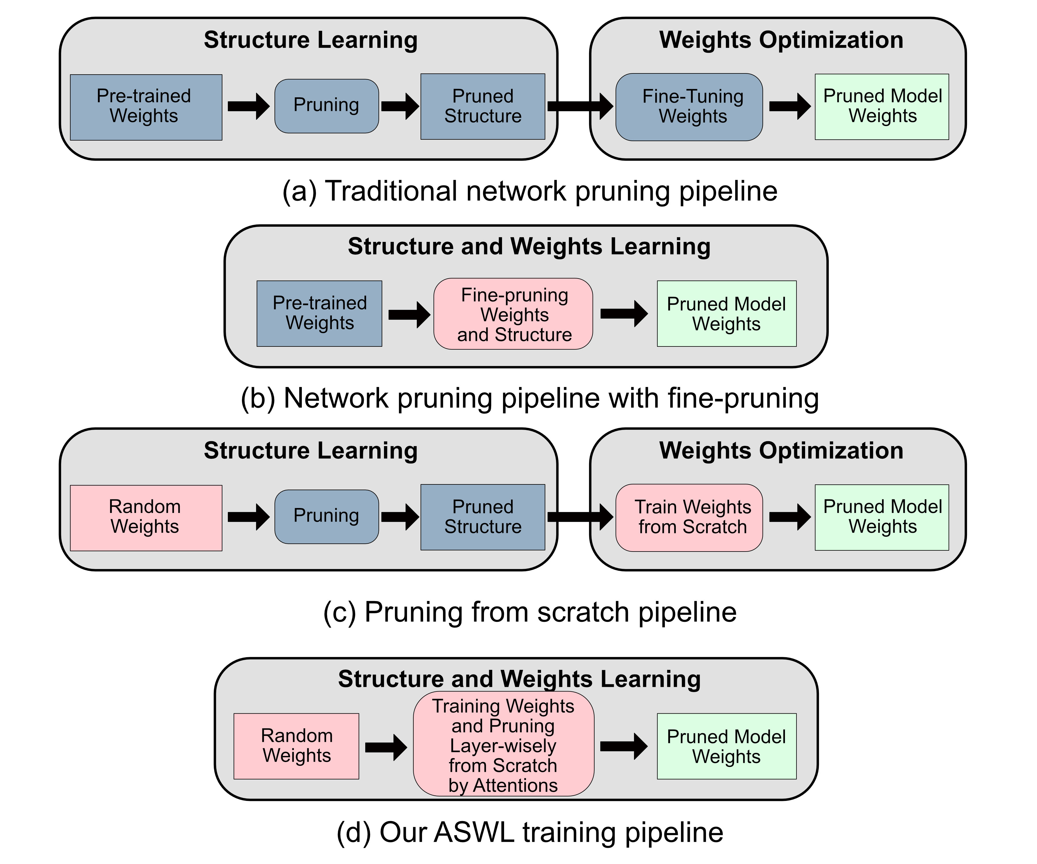
Figure 1: Comparison of neural network pruning pipelines. (a) Traditional network pruning learns pruned structure and fine-tunes from a pre-trained model. (b) Network fine-pruning learns both structure and weights jointly from a pre-trained model. (c) Pruning from scratch first generates a pruned structure and then trains the pruned model from randomly initialized weights. (d) ASWL learns both sparse structure and weights simultaneously through layer-wise attention from scratch in a unified procedure.

Pruning, which removes connections or neurons in a network, is one of the most popular network compression techniques. It reduces both the size and the computational complexity of a model since pruned weights do not need to be calculated or stored. Moreover, pruning is size-efficient as deep sparse models consistently outperform shallow dense models with almost no loss of or even a greater accuracy Zhu and Gupta (2017). When network pruning was first introduced for compression, redundant connections were pruned using a three-step pipeline illustrated in Fig. 1(a): first, the network is trained to learn which connections are important; next, the unimportant connections are pruned; finally, the network is retrained to fine-tune the weights of the remaining connections Han et al. (2015). The same three-step pipeline was later employed to perform layer-wise pruning in a layer-wise optimal brain surgeon Dong et al. (2017).

It was shown that structure learning and weights optimization could be combined to simplify the pruning process as Fig 1(b) shows. Fine-pruning Tung et al. (2017) proposed a principled method in which the pruning ratio of each layer is first predicted by the Bayesian optimization with a pre-trained network, and then the network is jointly fine-tuned and compressed with the predicted pruning ratios. The joint training was frequently used in quantization methods known as the Straight-Through Estimator (STE) Yin et al. (2019) to avoid zero gradients during back-propagation. The advantage of such a pipeline is that it allows the pruning status to adapt during the change of weights Tung and Mori (2018). However, pruning with pre-training is a time-consuming procedure. One needs to repeat pruning and fine-tuning several times to find a good sparse configuration Dettmers and Zettlemoyer (2019). In the meantime, using a reward function to find the pruning ratio for each layer is also an expensive procedure Zhou et al. (2019).

Later work, therefore, shows that the weights of a model and its pruned structure can be directly learned from randomly initialized weights (Fig. 1(c)). Pruning from Scratch Wang et al. (2020) proposed a novel network pruning pipeline that first learns the pruned structure directly from randomly initialized weights and then optimizes the weights of the pruned network. This kind of pipeline bypasses the time-consuming pre-training procedure. Nevertheless, the structure learning and weights optimization proceed separately here so that it only prunes weights based on fixed regularization before training the weights Liu et al. (2020).

Recently, the attention mechanism was brought into network pruning and achieved great success Yamamoto and Maeno (2018); Chin et al. (2020). In this paper, we propose a new pruning pipeline, Attention-based Simultaneous sparse structure and weight Learning (ASWL). As shown in Fig. 1(d), in ASWL, the layer-wise sparsity and weights are jointly learned from scratch in a unified training pipeline. Specifically, we first use the attention mechanism to learn the importance of each layer in a network and determine the corresponding pruning ratio. Then, we jointly prune the layer under the guidance of the pruning ratio and update the unpruned weights. The major contributions of our work are summarized as follows:

• ASWL provides a unified framework that combines both layer-wise pruning and weights optimization to learn a pruned network from randomly initialized weights. During ASWL training, both weights of the dense network and the sparse network are tracked so that the pruning ratio for each layer is simultaneously learned as the weights change.

• In ASWL, layer-wise pruning decisions are made through a novel attention-based approach. Attention scales in the attention mechanism are set across each layer instead of previous channel-wise or weight-wise attention mechanism. A pruning ratio is then directly computed based on the learned attention value for each layer.

• ASWL no longer needs the time-consuming pre-training procedure in network pruning but provides equivalent pruning results. Through extensive experiments on benchmark datasets, we demonstrate that ASWL leads to superior pruning results in terms of accuracy, network size, and operating efficiency when compared with state-of-the-art pruning methods.

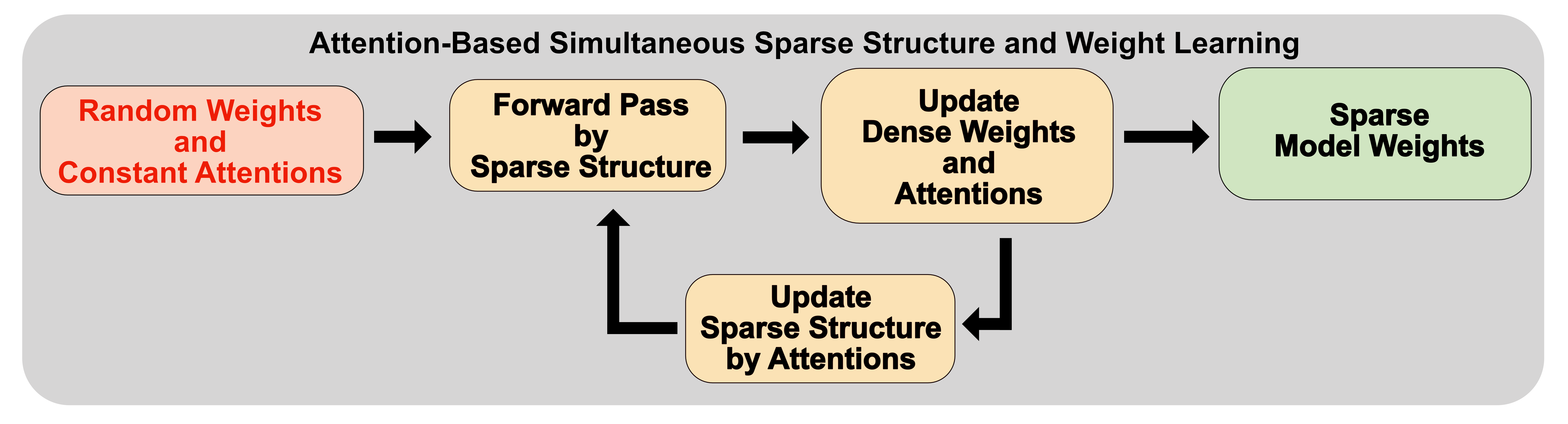
Figure 2: ASWL simultaneous training procedure with the attention mechanism.

2 Related Work

Neural network pruning techniques were used to avoid the overfitting problem in early work. For example, optimal brain surgeon Hassibi and Stork (1993) and dynamic sparsely connected artificial neural networks Ström (1997) pruned those connections that lead to a limited change of validation errors. The Dropout was introduced to prune or remove neurons randomly with a given ratio so that the complexity of the model is reduced. Later, pruning methods were employed to identify and remove unnecessary weights to reduce the size as well as the run-time latency of a targeted model. While some of the pruning methods like ThiNet Luo et al. (2017) and Stripe-wise Pruning Meng et al. (2020) prune feature maps or filter stripes, most others remove connections/neurons because sparse structures provided by unstructured pruning typically lead to a higher accuracy with a lower redundancy of weights Liu et al. (2020).

When pruning methods were first introduced to deep compression, they removed all connections whose weights were lower than a threshold Han et al. (2015). It was shown that pruning unimportant weights results in almost no loss of accuracy as the weights in deep neural networks are highly redundant. Then, methods were proposed to identify unnecessary weights layer-wisely Yang et al. (2017); Dong et al. (2017); Yu et al. (2018), which offers flexible pruning ratios on different layers and thus achieves better results. Automated Machine Learning (AutoML) was also introduced into pruning He et al. (2018), where the design space was efficiently sampled using reinforcement learning to find the best-pruned structure of a pre-trained model. Additionally, the attention mechanism was recently employed to find unimportant weights Hacene et al. (2019); Wu et al. (2018); Lin et al. (2019). Most of them introduced attention scales across each channel or each weight of the targeted layer. For example, LeGR-based pruning Chin et al. (2020) trained pairs of parameters (scale and shift) across each channel and then pruned output features accordingly.

More recently, the common three-step pruning pipeline, i.e., pre-training, pruning and fine-tuning, has been simplified. Fine-pruning Tung et al. (2017) jointly fine-tunes and compresses the pre-trained network with the pruning ratio of each layer predicted by the Bayesian optimization. Later, the lottery ticket hypothesis stated that dense randomly-initialized neural networks contain subnetworks, known as winning tickets, that reach accuracy equivalent to its original network with a similar number of training iterations Frankle and Carbin (2018). The hypothesis was mathematically proved in Malach et al. (2020). Based on such findings, Pruning from Scratch Wang et al. (2020) proposed to prune networks from randomly initialized weights. Specifically, it first learns the channel importance for each layer with a sparsity regularizer, then searches for a pruned structure with a method adopted from Network Slimming Liu et al. (2017) but used floating-point operations per second (FLOPS) as constraints. The pruned structure is then optimized from random weights. However, sanity-checking Su et al. (2020) showed that initial tickets are hard to be learned from the training data. Thus, it is necessary to keep the pruned structure flexible during training. To this end, more recent work trained sparse networks from scratch by regrowing some connections after a fixed number of iterations (e.g., per epoch) based on the gradient momentum, aka, sparse momentum, of the weights in these iterations Dettmers and Zettlemoyer (2019). Nonetheless, when one of the connections converges during training, its sparse momentum will also trend to zero, often leading to a sub-optimal structure and weights during the training.

3 Attention-based Simultaneous Learning

The objective of our new training pipeline, Attention-based Simultaneous sparse structure and weight Learning (ASWL), is to train both pruned structure and model weights from randomly initialized weights. Different from existing pruning methods, ASWL obtains layer-wise pruned deep learning models without pre-training. As shown in Fig. 2, we first convert a model into an attention-based model by replacing its traditional weighted layers with attention-based weighted layers. Instead of learning the pruned structure by regrowing connections after a fixed number of iterations, we pruned the weights layer-wise based on the pruning ratio calculated from the learned attention of the target layer in every iteration. In the mean time, the unpruned parameters are tracked and learned directly from the forward pass of the pruned structure. Such simultaneous learning tracks both pruned and unpruned weights during training and thus gives an adaptive pruning decision on the sparse structure.

3.1 Attention-based Neural Networks

The sparsity of a pruned network is weakly related to its output and hence is hardly to be learned directly Lin et al. (2020). Recent research shows that the attention mechanism provides a promising solution Yamamoto and Maeno (2018); Hacene et al. (2019). Unlike the traditional methods which set attention scalars channel-wisely or weight-wisely, we introduced a much simpler layer-wise attention mechanism, where an attention scalar value was defined across all $L$ layers in our attention-based neural network. Such model is denoted as $f(x;\mathbf{w},\mathbf{A})$ where $x$ is the input of the model, $\mathbf{w}$ is the traditional trainable weights, and $\mathbf{A}=\{a_{1},a_{2},...,a_{L}\}$ is the layer-wise attention values. Given a scalar gate value $a_{l}\in(0,1]$ for the $l^{th}$ layer as the attention, it is multiplied with the output of the layer. That is, assuming the output of the $l^{th}$ original layer is $f_{l}(x_{l-1};\mathbf{w}_{l})$, the attended output is modified as $\hat{f}_{l}(x_{l-1};\mathbf{w}_{l},a_{l})=a_{l}\cdot f_{l}(x_{l-1};\mathbf{w}_{l})$. Each attention value is initialized to 0.5 at the beginning. During training, both weights and attentions are updated. With pruning applied, the optimization objective of an attention-based neural network with compressed weights $\mathbf{\hat{w}}$ is:

$$\underset{\mathbf{\hat{w}},\mathbf{A}}{min}\sum_{i}^{N}{\mathfrak{L}(f(x_{i};\mathbf{\hat{w}},\mathbf{A}))}+\gamma\Psi(\mathbf{A})+\lambda\sum_{j}\mathbf{\hat{w}}_{j}^{2}$$ (1)

where $\mathfrak{L}(\cdot)$ denotes the cross-entropy loss, $\Psi(\cdot)$ is the sparsity regularizer for structure learning (discussed in the next section), L2 regularizer encourages all weights to be small Krogh and Hertz (1992), and $\gamma$ and $\lambda$ are the coefficients for the sparsity regularizer and L2 regularizer, respectively.

3.2 Pruning Ratios and Sparsity Regularizer

Layer-wise pruning methods typically require a pre-trained model as the starting point to search for a pruned structure. Recent work in Tung et al. (2017) and He et al. (2018) use naive Bayesian to optimize the pruning ratio layer-wisely in a given network. However, employing this kind of optimization in every training iteration is prohibitively time-consuming. In order to facilitate simultaneous optimization of structure and weights in each iteration, we propose a more efficient algorithm to calculate the pruning ratios directly from the attentions in our attention-based model.

Algorithm 1 Training Algorithm for Attention-based Simultaneous sparse structure and Weight Learning

1:function Train($iterations$, $\alpha$)

2:     $\mathbf{w},\mathbf{A}\leftarrow$ initialize()

3:

4:     for $i$ from 1 to $iterations$ do

5:         $\mathbf{p}\leftarrow(1-\mathbf{A})^{\alpha}$

6:         $\mathbf{\hat{w}}\leftarrow prune(\mathbf{w},\mathbf{p})$

7:

8:         $\mathbf{x}\leftarrow getNextBatch()$

9:         $\mathfrak{l}\leftarrow\sum_{i}^{N}{\mathfrak{L}(f(x_{i};\mathbf{\hat{w}},\mathbf{A}))}+\gamma\Psi(\mathbf{A})+\lambda\sum_{i}\mathbf{\hat{w}}_{i}^{2}$

10:

11:         $\mathbf{G}\leftarrow calculateGradients(\mathfrak{l};\mathbf{\hat{w}},\mathbf{A})$

12:         $\mathbf{w},\mathbf{A}\leftarrow updateWeights(\mathbf{G};\mathbf{w},\mathbf{A})$

13:     end for

14:end function

In Wang et al. (2020); Hacene et al. (2019), it was shown that scaling the network weights will suppress the unimportant ones, resulting in a pruning effect. As a result, the learned attentions can be used to represent the importance of each layer. That is, if a layer has a larger attention, it is considered to be more important so that it needs to be pruned less, and vice versa. Here, we introduce a positive hyper-parameter, the pruning factor $\alpha$, to gain more control when computing the pruning ratio $p_{l}$ based on the given attention $a_{l}$ of the $l^{th}$ layer:

$$p_{l}(a_{l})=(1-a_{l})^{\alpha},$$ (2)

where $a_{l}$ is the attention for the $l^{th}$ layer and $\alpha$ is the pruning factor. To ensure not all weights are pruned, we limited the maximum pruning ratio to be $99\%$. Since our attentions are applied along the layer dimension when weights are pruned, the overall sparsity $S$ of our attention-based model is computed as:

$$S(\mathbf{A})=\frac{\sum_{l}(1-p_{l}(a_{l}))n_{\mathbf{w}_{l}}}{\sum_{l}n_{\mathbf{w}_{l}}},$$ (3)

where $p_{l}$ is the pruning ratio and $n_{\mathbf{w}_{l}}$ is the total number of unpruned weights in the $l^{th}$ layer. Note that $n_{\mathbf{w}_{l}}$ is a constant as it is pre-determined for each layer.

Regularizers like L1 or L2 encourage the network weights $\mathbf{w}$ to be small, but not necessarily zeros. Thus, an additional regularizer is required in ASWL to encourage the pruning procedure to remove unimportant weights in each layer. Moreover, the L1/L2 regularizer encourages attentions to be zeroes without giving any consideration on the sparsity of the entire model, especially when the pruning factor is not set to 1. As a result, we adopted the sparsity regularizer proposed in Wang et al. (2020) as follows and combined it with L2 in ASWL:

$$\Psi(\mathbf{A})=S(\mathbf{A})^{2}$$ (4)

The square sparsity regularizer is differentiable Luo and Wu (2020) and will help minimize the layer-wise sparsity during optimization.

3.3 Simultaneous Sparse Structure Learning and Weight Optimization

Traditional pruning methods learn the pruned structure first, and then optimize the weights based on the pruned structure. The pruned structure can be easily found if a pre-trained model is available. However, with the weights training from random initialized values, efficient weights might change gradually from shallow to deep layers Dettmers and Zettlemoyer (2019). Meanwhile, a dense neural network contains a subnetwork that has the same accuracy even without fine-tuning Malach et al. (2020). These results motivated us to perform simultaneous learning on both the sparse structure and weights in ASWL by tracking both the dense network (through the backward propagation) and the sparse subnetwork (through the forward pass).

In ASWL training, both weights for the dense network and the sparse network are tracked so that the structure is simultaneously learned as the weights change. The parameters of the sparse network are pruned by removing at least the bottom $p_{i}$ percent dense weights in the $i_{th}$ layer based on the absolute weight values $|w_{i}|$. After training, the attention values are applied to the weights and discarded together with the weights in the dense network. Only the weights in the sparse network are stored.

Each training iteration in ASWL contains four steps: (1) the network classification loss is calculated through a forward pass based on the compressed weights $\mathbf{\hat{w}}$ and attentions $\mathbf{A}$, (2) both uncompressed weights $\mathbf{w}$ and attentions $\mathbf{A}$ are updated through back-propagation, (3) the pruning ratio $\mathbf{p}$ is computed by the new attentions $\mathbf{A}$ and the pruning factor $\alpha$, and (4) the model is compressed layer-wise using the pruning ratio $\mathbf{p}$, and the compressed weights $\mathbf{\hat{w}}$ are updated. The detailed training procedure is summarized in Algorithm 1. In ASWL, through simultaneous optimization, weights that have been pruned at first may be recovered later, and the weights defined as important at first can be pruned, all depending on the evolution of the network structure.

4 Experimental Results

In this section, we perform extensive experiments with ASWL on VGG-16 Simonyan and Zisserman (2014), ResNet50 He et al. (2016), and MobileNetV2 Sandler et al. (2018). For VGG-16 and ResNet50, we simply replace the traditional convolutional layer and dense layer with our attention-based convolutional layer and dense layer. For MobileNetV2, we replace the $1\times 1$ point-wise convolutional layer with an attention-based convolutional layer but left the depth-wise layer uncompressed since 99% of the parameters and calculations are contained in point-wise convolutional layers. There are totally three hyperparameters in ASWL: the coefficients of sparsity and L2 regularizer ($\gamma$ and $\lambda$), and the pruning factor $\alpha$. They are specified later in different experiments.

Our ASWL training pipeline was implemented in TensorFlow Abadi et al. (2016). All models are trained on a computer with Intel i7 8700K CPU, 16GB RAM, and two NVIDIA RTX 2080 Ti graphic cards, each of which has 11GB of GDDR SDRAM. The source code of this work is available in the supplemental materials with detailed comments and will be made publicly available after the review period of AAAI 2022.

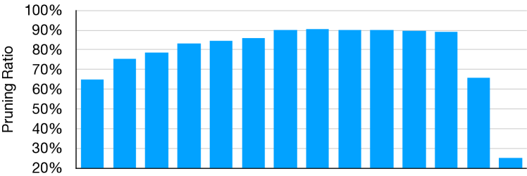
(a) Pruning details for VGG-16 with $\alpha=1.5$

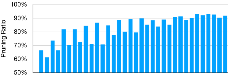
(b) Pruning details for MobileNetV2 with $\alpha=1$

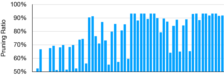
(c) Pruning details for ResNet56 with $\alpha=1$

Figure 3: Layer-wise pruning details on MNIST for (a) VGG-16 with $\alpha=1.5$, where the last two layers are attention-based dense layers, and all others are attention-based convolutional layers, (b) MobileNetV2 with $\alpha=1$, where the first layer is an attention-based convolutional layer with a $3\times 3$ filter, and others are point-wise ($1\times 1$ filter) attention-based convolutional layers, (c) ResNet56 with $\alpha=1$, where the last layer is an attention-based dense layer, and others are attention-based convolutional layer.

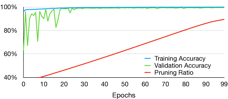
(a) Training graph for VGG16 with $\alpha=1.5$

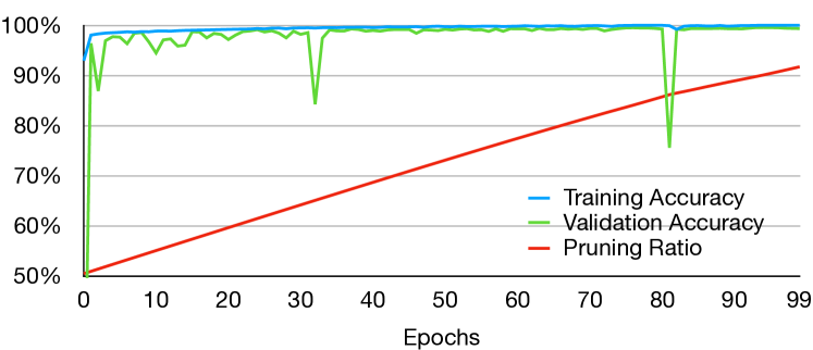
(b) Training graph for MobileNetV2 with $\alpha=1$

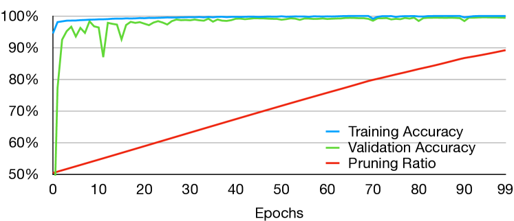
(c) Training graph for ResNet56 with $\alpha=1$

Figure 4: MNIST Training graph: training accuracy (blue line), validation accuracy (green line), and pruning ratio (red line) for (a) VGG-16 with $\alpha=1.5$, (b) MobileNetV2 with $\alpha=1$, and (c) ResNet56 with $\alpha=1$.

Specifically, we conducted our experiments on the standard MNIST LeCun et al. (1998), Cifar-10 Krizhevsky and Hinton (2009) and ImageNet (ILSVRC-2012 in version 2.0.1) Russakovsky et al. (2015) datasets and compared with the following pruning methods: Learning both Weights and Connections for Efficient Neural Networks (ENN) Han et al. (2015), Rethingking Network Pruning (RNP) Liu et al. (2018), Discrimination-aware Channel Pruning (DCP) Zhuang et al. (2018), Convolutional neural network pruning with structural redundancy reduction (SRR) Wang et al. (2021), Network Pruning via Performance Maximization (NPPM) Gao et al. (2021), Learned Threshold Pruning (LTP) Azarian et al. (2020), Pruning from Scratch (PFS) Wang et al. (2020), Dynamic Sparse Reparameterization (DS) Mostafa and Wang (2019), Pruning Filter in Filter (PFF) Meng et al. (2020), WoodFisher (WF) Singh and Alistarh (2020), Sparse Networks from Scratch (SNS) Dettmers and Zettlemoyer (2019), and Dynamic Pruning with Feedback (DPF) Lin et al. (2020).

Model	Pruning Factor	Baseline	$\Delta$ Accuracy	Pruning Ratio
	$\alpha$	$\%$	$\%$	$\%$
VGG16-1	1	99.51%	+0.04%	90.69%
VGG16-1.5	1.5		+0.09%	88.56%
VGG16-2	2		+0.03%	87.19%
MobileNetV2-1	1	99.56%	+0.00%	90.10%
MobileNetV2-1.5	1.5		-0.07%	86.32%
MobileNetV2-2	2		-0.09%	82.03%
ResNet56-1	1	99.50%	+0.07%	87.74%
ResNet56-1.5	1.5		+0.00%	83.70%
ResNet56-2	2		+0.05%	75.61%

Table 1: ASWL training results with different pruning factors on VGG-16 (top row), MobileNetV2 (middle row), and ResNet50 (bottom row) for MNIST.

Model	Pruning Factor	Baseline	$\Delta$ Accuracy	Pruning Ratio
	$\alpha$	$\%$	$\%$	$\%$
VGG16-1	1	92.64	+0.50%	93.80%
VGG16-1.5	1.5		+0.76%	91.96%
VGG16-2	2		+0.18%	78.11%
MobileNetV2-1	1	93.14	+0.27%	95.86%
MobileNetV2-1.5	1.5		+0.41%	94.61%
MobileNetV2-2	2		+0.11%	78.89%
ResNet56-1	1	93.44	+0.28%	95.97%
ResNet56-1.5	1.5		+0.10%	94.86%
ResNet56-2	2		+0.26%	96.19%

Table 2: ASWL training results with different pruning factors on VGG-16 (top row), MobileNetV2 (middle row), and ResNet56 (bottom row) for Cifar10.

Model	Method	Simu.	From	Unstructured	Baseline	$\Delta$ Acc.	Pr. Ratio
		Training	Scratch	Pruning	%	%	%
VGG16	DCP	$\times$	$\times$	$\times$	93.80%	+0.17%	52.1%
	RNP	$\times$	$\times$	$\checkmark$	93.76%	-0.04%	80.0%
	PFS	$\times$	$\checkmark$	$\times$	93.44%	+0.19%	93.6%
	PFF	$\times$	$\checkmark$	$\times$	93.25	-0.40%	92.7%
	SNS	$\circ$	$\checkmark$	$\checkmark$	93.51%	-0.50%	95.0%
	ASWL (Ours)	$\boldsymbol{\checkmark}$	$\boldsymbol{\checkmark}$	$\boldsymbol{\checkmark}$	92.81%	+0.76%	92.0%
ResNet56	DCP	$\times$	$\times$	$\times$	93.80%	-0.31%	92.8%
	RNP	$\times$	$\times$	$\checkmark$	93.80%	-0.31%	93.1%
	PFS	$\times$	$\checkmark$	$\times$	93.23%	-0.18%	93.1%
	PFF	$\times$	$\checkmark$	$\times$	93.10%	+0.12%	77.7%
	DPF-90	$\checkmark$	$\checkmark$	$\checkmark$	94.51%	-0.56%	90.0%
	DPF-95	$\checkmark$	$\checkmark$	$\checkmark$	94.51%	-1.26%	95.0%
	ASWL (Ours)	$\boldsymbol{\checkmark}$	$\boldsymbol{\checkmark}$	$\boldsymbol{\checkmark}$	93.44%	+0.28%	96.0%

Table 3: ASWL training results on Cifar10, and the comparison with state-of-the-art network pruning methods. In the “simultaneous training” column, $\times$ indicates static pruned structure during training, $\circ$ indicates that the network connections are iteratively regrown after a fixed number of iterations (e.g., every epoch), and $\checkmark$ indicates fully simultaneous structure and weight training. In the “from scratch” column, $\times$ indicates pruning from pre-trained, and $\checkmark$ indicates pruning from scratch. In the “unstructured pruning” column, $\times$ indicates structured pruning, and $\checkmark$ indicates unstructured. For each method, accuracy, and pruning ratio are reported, and the best results are highlighted in bold. The same applies to Table 4

.

4.1 Results on MNIST

We first trained selected models with ASWL on MNIST, which contains 10 different handwriting digits with 60,000 training images and 10,000 testing images. Each of the models was trained with various pruning factors of 1, 1.5, and 2 for 100 epochs by the Adam optimizer at a learning rate of 0.001 and 0.98 decay for each epoch. The attentions of each layer are initialized at 0.5. The hyper-parameter $\gamma$ (the sparsity regularizer coefficient) is used mainly to achieve a desired pruning ratio and set at 0.5 for all models. Following Simonyan and Zisserman (2014), He et al. (2016), and Sandler et al. (2018), the other hyper-parameter $\lambda$ (the L2 regularizer coefficient) is set at $5\cdot 10^{-4}$, $0.0001$, and $0.00004$ for VGG16, ResNet 56, MobileNetV2, respectively. The models with the best results are selected.

Table 1 shows the ASWL training results on MNIST with VGG16 (Top), MobileNetV2 (Middle), and ResNet56 (Bottom). In most situations, the pruning ratio progressively increases when we reduce the pruning factor. There is no obvious relation found between model accuracy and pruning factors, while a smaller pruning factor offers a greater pruning ratio. With about $10\%$ to $25\%$ of weights in the original dense models, our ASWL provides similar or many times higher accuracy.

Fig. 3 (a) shows the pruning details of each layer in VGG-16 with a pruning factor of $\alpha=1.5$. Deeper attention-based convolutional layers are pruned more than the shallower ones, while the last two attention-based dense layers have pruning ratios much less than the convolutional layers. Fig. 3 (b) demonstrates the pruning ratio of each regular (non depth-wise) attention-based convolutional layer in MobileNetV2 with a pruning factor of $\alpha=1$. Its first convolutional layer with a filter size of $3\times 3$ has the least pruning ratio, just above $50\%$. Meanwhile, pruning ratios appear to be greater in deeper convolutional layers, similar to the VGG-16 case. The layer-wise pruning details of ResNet56 are shown in Fig. 3 (c), where the last layer is an attention-based dense layer. ResNet56 has much more layers compared with VGG-16 and MobileNetV2 but still has an obvious trend of a higher pruning ratio for a deeper layer. Fig. 4 (a) shows the training graph of VGG-16 with a pruning factor of $\alpha=1.5$. Overall, the pruning ratio continues increasing as the model is being trained, and the validation accuracy stabilizes after 30 epochs. We observe the same in the training graphs of MobileNetV2 with $\alpha=1$ and ResNetV2 with $\alpha=1$ (Fig. 4 (b) and (c)).

4.2 Results on Cifar10

Cifar10 is a dataset that contains 10 different classes with 50,000 training images and 10,000 testing images. Similar to our experiment on MNIST, we trained the selected models with various pruning ratios of 1, 1.5, and 2. For VGG16, we used an initial learning rate of 0.1 and multiplied 0.5 for every 20 epochs with the SGD optimizer (momentum 0.9), and trained for 250 epochs at a batch size of 128. For ResNet 56, we followed the same settings in He et al. (2016). For MobileNetV2, we trained for 350 epochs on SGD optimizer with an initial learning rate of 0.1, which was divided by 10 after 150 and 250 epochs. Again, the hyper-parameter $\gamma$ (sparsity regularizer coefficient) is used to help us achieve a desired pruning ratio and was set at 2.5, 5 and 0.5 for VGG16, ResNet 56, MobileNetV2, respectively. Following Simonyan and Zisserman (2014), He et al. (2016), Sandler et al. (2018), the other hyper-parameter $\lambda$ is set at $5\cdot 10^{-4}$, $0.0001$, and $0.00004$ for VGG16, ResNet 56, and MobileNetV2, respectively. The models with the best results are selected.

Table 2 shows the ASWL training results on Cifar10 with VGG16 (Top), MobileNetV2 (Middle), and ResNet56 (Bottom). Similar to MNIST, the results show that small pruning factors typically lead to higher pruning ratios. Additionally, we observe that ASWL offers an improvement on model accuracy with reduced network size and higher run-time efficiency over uncompressed baselines in all cases. The pruning details of the three models the three models are shown in Fig. 1 in supplemental materials. Similar to the case of MNIST, deeper layers are pruned more than the shallower ones except for the last dense layer for classification. Similar training graphs (Fig. 2 in supplemental materials) of the three models were observed as in MNIST that the model converges after about 30 epochs and reaches the highest validation accuracy at around 130 epochs, at which time the overall pruning ratio stops increasing as well.

Table 3 compares ASWL with state-of-the-art pruning methods on Cifar10 with ResNet56 (top) and VGG16 (bottom). Clearly, ASWL achieved a higher accuracy than the baseline on both models. Overall, our ASWL model achieved an outstanding pruning ratio with the highest increase of accuracy when compared to the baseline. These results clearly demonstrate the advantages of simultaneous training and layer-wise attention-based pruning in ASWL.

Method	Simu.	From	Unstructured	Baseline	T1 Acc.	Pr. Ratio
	Training	Scratch	Pruning	%	%	%
ENN	$\times$	$\times$	$\checkmark$	76.1%	76.1%	60.0%
CP 0.5$\times$	$\times$	$\times$	$\times$		75.4%	48.5%
SRR	$\times$	$\times$	$\times$		75.1%	55.1% (FLOPS)
PFS 0.75$\times$	$\times$	$\checkmark$	$\times$		75.6%	63.9%
DS-20	$\circ$	$\checkmark$	$\checkmark$		73.3%	80.0%
SNS-20	$\circ$	$\checkmark$	$\checkmark$		73.8%	80.0%
NPPM	$\checkmark$	$\checkmark$	$\times$		76.0%	56.0% (FLOPS)
LTP	$\checkmark$	$\times$	$\checkmark$		73.3%	85.6%
WF-90	$\checkmark$	$\times$	$\checkmark$		75.2%	90.0%
DPF-80	$\checkmark$	$\checkmark$	$\checkmark$		75.5%	73.5%
DPF-90	$\checkmark$	$\checkmark$	$\checkmark$		74.6%	82.6%
ASWL (Ours)	$\boldsymbol{\checkmark}$	$\boldsymbol{\checkmark}$	$\boldsymbol{\checkmark}$		76.5%	86.1%

Table 4: ASWL training result for ResNet-50 on ImageNet, and the comparison with state-of-the-art network pruning methods. Pruning ratio with FLOPS indicates the pruning ratio of the target method is calculated by FLOPS instead of number of weights.

4.3 Results on ImageNet

Compared with MNIST and Cifar10, ImageNet is a much larger dataset that contains 1000 classes with 1.2M training images and 50K testing images. We trained ResNet-50 using ASWL following the same training setting in He et al. (2016) for ResNet-50. The hyper-parameter $\gamma$ was set at 0.5. Additionally, the pruning factor was set to 1. The models with the best results are selected.

Table 4 compares ASWL with state-of-the-art pruning methods on ResNet-50. Through simultaneous training with layer-wise pruning from randomly initialized weights, ASWL achieves the top-1 accuracy of $76.5\%$ with a great pruning ratio ($86.1\%$). Note that this accuracy is higher than the uncompressed ResNet-50 baseline model ($76.1\%$). Considering the balance between the top-1 accuracy and the pruning ratio, ASWL provides a superior pruning result when compared to all existing pruning methods. If we consider accuracy alone, it is the second best.

5 Conclusion

In this paper, we proposed a novel pruning pipeline, Attention-based Simultaneous sparse structure and weight Learning (ASWL). In ASWL, we first use the attention mechanism to learn the importance of each layer in a network and determine the corresponding pruning ratio. Then, the layer-wise sparsity and weights are jointly learned from scratch in a unified training procedure. Our extensive experiments on benchmark datasets show that ASWL achieves outstanding pruning results in terms of accuracy, pruning ratio, and operating efficiency.

References

- Russakovsky et al. [2015] Olga Russakovsky, Jia Deng, Hao Su, Jonathan Krause, Sanjeev Satheesh, Sean Ma, Zhiheng Huang, Andrej Karpathy, Aditya Khosla, and Michael Bernstein. Imagenet large scale visual recognition challenge. International journal of computer vision, 115(3):211–252, 2015. ISSN 0920-5691.
- He et al. [2016] Kaiming He, Xiangyu Zhang, Shaoqing Ren, and Jian Sun. Deep residual learning for image recognition. In Proceedings of the IEEE conference on computer vision and pattern recognition, pages 770–778, 2016.
- Ren et al. [2015] Shaoqing Ren, Kaiming He, Ross Girshick, and Jian Sun. Faster r-cnn: Towards real-time object detection with region proposal networks. In Advances in neural information processing systems, pages 91–99, 2015.
- He et al. [2017] Kaiming He, Georgia Gkioxari, Piotr Dollár, and Ross Girshick. Mask r-cnn. In Proceedings of the IEEE international conference on computer vision, pages 2961–2969, 2017.
- Noh et al. [2015] Hyeonwoo Noh, Seunghoon Hong, and Bohyung Han. Learning deconvolution network for semantic segmentation. In Proceedings of the IEEE international conference on computer vision, pages 1520–1528, 2015.
- Salehinejad and Valaee [2020] Hojjat Salehinejad and Shahrokh Valaee. Edropout: Energy-based dropout and pruning of deep neural networks. arXiv preprint arXiv:2006.04270, 2020.
- Howard et al. [2017] Andrew G Howard, Menglong Zhu, Bo Chen, Dmitry Kalenichenko, Weijun Wang, Tobias Weyand, Marco Andreetto, and Hartwig Adam. Mobilenets: Efficient convolutional neural networks for mobile vision applications. arXiv preprint arXiv:1704.04861, 2017.
- Iandola et al. [2016] Forrest N Iandola, Song Han, Matthew W Moskewicz, Khalid Ashraf, William J Dally, and Kurt Keutzer. Squeezenet: Alexnet-level accuracy with 50x fewer parameters and< 0.5 mb model size. arXiv preprint arXiv:1602.07360, 2016.
- Krizhevsky et al. [2012] Alex Krizhevsky, Ilya Sutskever, and Geoffrey E Hinton. Imagenet classification with deep convolutional neural networks. In Advances in neural information processing systems, pages 1097–1105, 2012.
- Zhu and Gupta [2017] Michael Zhu and Suyog Gupta. To prune, or not to prune: exploring the efficacy of pruning for model compression. arXiv preprint arXiv:1710.01878, 2017.
- Han et al. [2015] Song Han, Jeff Pool, John Tran, and William Dally. Learning both weights and connections for efficient neural network. In Advances in neural information processing systems, pages 1135–1143, 2015.
- Dong et al. [2017] Xin Dong, Shangyu Chen, and Sinno Pan. Learning to prune deep neural networks via layer-wise optimal brain surgeon. In Advances in Neural Information Processing Systems, pages 4857–4867, 2017.
- Tung et al. [2017] Frederick Tung, Srikanth Muralidharan, and Greg Mori. Fine-pruning: Joint fine-tuning and compression of a convolutional network with bayesian optimization. arXiv preprint arXiv:1707.09102, 2017.
- Yin et al. [2019] Penghang Yin, Jiancheng Lyu, Shuai Zhang, Stanley Osher, Yingyong Qi, and Jack Xin. Understanding straight-through estimator in training activation quantized neural nets. arXiv preprint arXiv:1903.05662, 2019.
- Tung and Mori [2018] Frederick Tung and Greg Mori. Clip-q: Deep network compression learning by in-parallel pruning-quantization. In Proceedings of the IEEE Conference on Computer Vision and Pattern Recognition, pages 7873–7882, 2018.
- Dettmers and Zettlemoyer [2019] Tim Dettmers and Luke Zettlemoyer. Sparse networks from scratch: Faster training without losing performance. arXiv preprint arXiv:1907.04840, 2019.
- Zhou et al. [2019] Daquan Zhou, Xiaojie Jin, Kaixin Wang, Jianchao Yang, and Jiashi Feng. Deep model compression via filter auto-sampling. arXiv preprint arXiv:1907.05642, 2019.
- Wang et al. [2020] Yulong Wang, Xiaolu Zhang, Lingxi Xie, Jun Zhou, Hang Su, Bo Zhang, and Xiaolin Hu. Pruning from scratch. In AAAI, pages 12273–12280, 2020.
- Liu et al. [2020] Ning Liu, Xiaolong Ma, Zhiyuan Xu, Yanzhi Wang, Jian Tang, and Jieping Ye. Autocompress: An automatic dnn structured pruning framework for ultra-high compression rates. In AAAI, pages 4876–4883, 2020.
- Yamamoto and Maeno [2018] Kohei Yamamoto and Kurato Maeno. Pcas: Pruning channels with attention statistics for deep network compression. arXiv preprint arXiv:1806.05382, 2018.
- Chin et al. [2020] Ting-Wu Chin, Ruizhou Ding, Cha Zhang, and Diana Marculescu. Towards efficient model compression via learned global ranking. In Proceedings of the IEEE/CVF Conference on Computer Vision and Pattern Recognition, pages 1518–1528, 2020.
- Hassibi and Stork [1993] Babak Hassibi and David G Stork. Second order derivatives for network pruning: Optimal brain surgeon. In Advances in neural information processing systems, pages 164–171, 1993.
- Ström [1997] Nikko Ström. Phoneme probability estimation with dynamic sparsely connected artificial neural networks. The Free Speech Journal, 5(1-41):2, 1997.
- Luo et al. [2017] Jian-Hao Luo, Jianxin Wu, and Weiyao Lin. Thinet: A filter level pruning method for deep neural network compression. In Proceedings of the IEEE international conference on computer vision, pages 5058–5066, 2017.
- Meng et al. [2020] Fanxu Meng, Hao Cheng, Ke Li, Huixiang Luo, Xiaowei Guo, Guangming Lu, and Xing Sun. Pruning filter in filter. arXiv preprint arXiv:2009.14410, 2020.
- Yang et al. [2017] Tien-Ju Yang, Yu-Hsin Chen, and Vivienne Sze. Designing energy-efficient convolutional neural networks using energy-aware pruning. In Proceedings of the IEEE Conference on Computer Vision and Pattern Recognition, pages 5687–5695, 2017.
- Yu et al. [2018] Ruichi Yu, Ang Li, Chun-Fu Chen, Jui-Hsin Lai, Vlad I Morariu, Xintong Han, Mingfei Gao, Ching-Yung Lin, and Larry S Davis. Nisp: Pruning networks using neuron importance score propagation. In Proceedings of the IEEE Conference on Computer Vision and Pattern Recognition, pages 9194–9203, 2018.
- He et al. [2018] Yihui He, Ji Lin, Zhijian Liu, Hanrui Wang, Li-Jia Li, and Song Han. Amc: Automl for model compression and acceleration on mobile devices. In Proceedings of the European Conference on Computer Vision (ECCV), pages 784–800, 2018.
- Hacene et al. [2019] Ghouthi Boukli Hacene, Carlos Lassance, Vincent Gripon, Matthieu Courbariaux, and Yoshua Bengio. Attention based pruning for shift networks. arXiv preprint arXiv:1905.12300, 2019.
- Wu et al. [2018] Bichen Wu, Alvin Wan, Xiangyu Yue, Peter Jin, Sicheng Zhao, Noah Golmant, Amir Gholaminejad, Joseph Gonzalez, and Kurt Keutzer. Shift: A zero flop, zero parameter alternative to spatial convolutions. In Proceedings of the IEEE Conference on Computer Vision and Pattern Recognition, pages 9127–9135, 2018.
- Lin et al. [2019] Shaohui Lin, Rongrong Ji, Chenqian Yan, Baochang Zhang, Liujuan Cao, Qixiang Ye, Feiyue Huang, and David Doermann. Towards optimal structured cnn pruning via generative adversarial learning. In Proceedings of the IEEE/CVF Conference on Computer Vision and Pattern Recognition, pages 2790–2799, 2019.
- Frankle and Carbin [2018] Jonathan Frankle and Michael Carbin. The lottery ticket hypothesis: Finding sparse, trainable neural networks. arXiv preprint arXiv:1803.03635, 2018.
- Malach et al. [2020] Eran Malach, Gilad Yehudai, Shai Shalev-Shwartz, and Ohad Shamir. Proving the lottery ticket hypothesis: Pruning is all you need. arXiv preprint arXiv:2002.00585, 2020.
- Liu et al. [2017] Zhuang Liu, Jianguo Li, Zhiqiang Shen, Gao Huang, Shoumeng Yan, and Changshui Zhang. Learning efficient convolutional networks through network slimming. In Proceedings of the IEEE International Conference on Computer Vision, pages 2736–2744, 2017.
- Su et al. [2020] Jingtong Su, Yihang Chen, Tianle Cai, Tianhao Wu, Ruiqi Gao, Liwei Wang, and Jason D Lee. Sanity-checking pruning methods: Random tickets can win the jackpot. arXiv preprint arXiv:2009.11094, 2020.
- Lin et al. [2020] Tao Lin, Sebastian U. Stich, Luis Barba, Daniil Dmitriev, and Martin Jaggi. Dynamic model pruning with feedback. In International Conference on Learning Representations, 2020.
- Krogh and Hertz [1992] Anders Krogh and John A Hertz. A simple weight decay can improve generalization. In Advances in neural information processing systems, pages 950–957, 1992.
- Luo and Wu [2020] Jian-Hao Luo and Jianxin Wu. Autopruner: An end-to-end trainable filter pruning method for efficient deep model inference. Pattern Recognition, 107:107461, 2020.
- Simonyan and Zisserman [2014] Karen Simonyan and Andrew Zisserman. Very deep convolutional networks for large-scale image recognition. arXiv preprint arXiv:1409.1556, 2014.
- Sandler et al. [2018] Mark Sandler, Andrew Howard, Menglong Zhu, Andrey Zhmoginov, and Liang-Chieh Chen. Mobilenetv2: Inverted residuals and linear bottlenecks. In Proceedings of the IEEE Conference on Computer Vision and Pattern Recognition, pages 4510–4520, 2018.
- Abadi et al. [2016] Martín Abadi, Ashish Agarwal, Paul Barham, Eugene Brevdo, Zhifeng Chen, Craig Citro, Greg S Corrado, Andy Davis, Jeffrey Dean, and Matthieu Devin. Tensorflow: Large-scale machine learning on heterogeneous distributed systems. arXiv preprint arXiv:1603.04467, 2016.
- LeCun et al. [1998] Yann LeCun, Corinna Cortes, and Christopher JC Burges. The mnist database of handwritten digits, 1998. URL http://yann. lecun. com/exdb/mnist, 10:34, 1998.
- Krizhevsky and Hinton [2009] Alex Krizhevsky and Geoffrey Hinton. Learning multiple layers of features from tiny images. 2009.
- Liu et al. [2018] Zhuang Liu, Mingjie Sun, Tinghui Zhou, Gao Huang, and Trevor Darrell. Rethinking the value of network pruning. arXiv preprint arXiv:1810.05270, 2018.
- Zhuang et al. [2018] Zhuangwei Zhuang, Mingkui Tan, Bohan Zhuang, Jing Liu, Yong Guo, Qingyao Wu, Junzhou Huang, and Jinhui Zhu. Discrimination-aware channel pruning for deep neural networks. In Advances in Neural Information Processing Systems, pages 875–886, 2018.
- Wang et al. [2021] Zi Wang, Chengcheng Li, and Xiangyang Wang. Convolutional neural network pruning with structural redundancy reduction. In Proceedings of the IEEE/CVF Conference on Computer Vision and Pattern Recognition, pages 14913–14922, 2021.
- Gao et al. [2021] Shangqian Gao, Feihu Huang, Weidong Cai, and Heng Huang. Network pruning via performance maximization. In Proceedings of the IEEE/CVF Conference on Computer Vision and Pattern Recognition, pages 9270–9280, 2021.
- Azarian et al. [2020] Kambiz Azarian, Yash Bhalgat, Jinwon Lee, and Tijmen Blankevoort. Learned threshold pruning. arXiv preprint arXiv:2003.00075, 2020.
- Mostafa and Wang [2019] Hesham Mostafa and Xin Wang. Parameter efficient training of deep convolutional neural networks by dynamic sparse reparameterization. arXiv preprint arXiv:1902.05967, 2019.
- Singh and Alistarh [2020] Sidak Pal Singh and Dan Alistarh. Woodfisher: Efficient second-order approximation for neural network compression. arXiv e-prints, pages arXiv–2004, 2020.