SVD-Embedded Deep Autoencoder for
MIMO Communications

Abstract

Using a deep autoencoder (DAE) for end-to-end communication in multiple-input multiple-output (MIMO) systems is a novel concept with significant potential. DAE-aided MIMO has been shown to outperform singular-value decomposition (SVD)-based precoded MIMO in terms of bit error rate (BER). This paper proposes embedding left- and right-singular vectors of the channel matrix into DAE encoder and decoder to further improve the performance of the MIMO DAE. SVD-embedded DAE largely outperforms theoretic linear precoding in terms of BER. This is remarkable since it demonstrates that DAEs have significant potential to exceed the limits of current system design by treating the communication system as a single, end-to-end optimization block. Based on the simulation results, at SNR=10dB, the proposed SVD-embedded design can achieve a BER of about $10^{-5}$ and reduce the BER at least 10 times compared with existing DAE without SVD, and up to 18 times compared with theoretical linear precoding. We attribute this to the fact that the proposed DAE can match the input and output as an adaptive modulation structure with finite alphabet input. We also observe that adding residual connections to the DAE further improves the performance.

I Introduction

The fundamental functionality of communication systems is to effectively transmit a message from a source to a destination over a channel. A well-established principle of communication systems design is to break up the system into multiple blocks, each with a specific responsibility, for instance, source coding, channel coding, precoding, modulation, and equalization, etc., and design them separately. The fact that each block therein can be independently designed and optimized makes the system design simpler, but such a split-up optimization is not globally optimal at the system level [1].

Deep learning (DL)-based end-to-end communications system [1], on the other hand, provides a new perspective to communications system design and aims to jointly optimize the components at the transmitter and receiver without any handcraft block structure. Unlike today’s system design which carries decades of research and implementation efforts, DL-based communication is still in its infancy stage. The simplicity and potential of this new system design approach are appealing and motivate us to exploit the potential of the end-to-end communications system design in the physical layer.

Recent attempts on DL in the physical layer for the single-input single-output channel have shown that, as a refreshing communication system design method, autoencoder (AE) can jointly optimize encoding, decoding, and signal representation [1, 2, 3]. AE is an artificial neural network that learns to match its output to its input. It has an encoder and decoder and tries to reconstruct the original input by minimizing the reconstruction error often through some impairment such as lossy or compressive representation. So, AE is an unsupervised learning approach. As such, it is intriguing how it improves the overall performance of communication systems in terms of bit error rate (BER). A deep autoencoder (DAE) ia an AE with a deep neural network. DAEs can be used for transmitter and receiver design. In [1], it is shown that DAE reaches the same block error rate as binary phase-shift keying (BPSK) modulation with Hamming (7,4) code and outperforms uncoded BPSK. The authors in [2] implemented the DAE on hardware. DAE can also significantly outperform convolutional codes in the high signal-to-noise ratio (SNR) [3].

DAE design is more challenging when it comes to multiple-input multiple-output (MIMO) systems. DAE in MIMO communication systems was first investigated in [4] where a MIMO spatial multiplexing system using DAE is designed with the perfect knowledge of channel state information at the transmitter (CSIT). The DAE takes advantage of CSIT to cancel interference at the receiver, and can be seen as decorrelator/interference nuller the same role singular-value decomposition (SVD) plays in MIMO systems [5]. Later, the authors in [6] applied channel state information at the receiver (CSIR), which improves the performance in terms of symbol error rate (SER).

I-A Contributions

In this paper, we focus on DAE design for MIMO communication with perfect CSIR and CSIT. We introduce an SVD-embedded DAE which improves the state-of-the-art DAE in terms of BER. The contributions of this paper can be summarized as follows:

• We propose and design an SVD-embedded DAE network. Precoding and pre-processing at the transmitter and receiver have been added as one layer with non-trainable weights. This design can achieve BER nearly $10^{-5}$ at SNR=10dB, and can reduce the BER 10 to 30 times compared with the plain DAE without any precoding layers. The encoder of SVD-embedded DAE uses the transmitted bits/symbols along with the CSIT as inputs, and its decoder exploits both the received symbols and the CSIR.

• Remarkably, the designed DAE outperforms the SVD precoding MIMO system from 1.5 to 18 times on BER depending on the SNR value. We attribute this amazing result to the fact that the SVD-embedded DAE can optimize and match the input and output symbols like an adaptive modulation structure to fit the precoding and presumably the target information rates corresponding to each eigenvalue/eigenmode channel, whereas the conventional methods use a block-based system optimization structure, which is known to be sub-optimal even if we know optimal solutions in each block.

• We test the performance of per-bit input and per-bit output regression and compare it with the commonly-used one-hot input and one-hot output [4, 6]. From our simulation, bit input is a good candidate for DAE especially when the number of input bits is 2 and 4. On the other hand, the one-hot input has a great potential for 6-bit input at high SNR.

• We add residual connections, i.e., shortcuts, in the proposed DAE. This design helps improve the performance, especially for the bit inputs. Instead of widening the network, the shortcuts can increase the learning capacity and performance of the network without extra parameters. It keeps the network with previous layer parameters, which may reduce the effect of the vanishing gradient problem. A skip connection helps preserve gradient and allows it to learn representations at different depths.

I-B Related Work

The DL has been exploited for improving the performance of many physical layer communication components, such as channel coding [7], channel modeling [8], precoding [9, 10], and massive MIMO [10, 11]. Besides, DAE for end-to-end communication has attracted increasing interest in various communications problems. DAE, as a semi-supervised learning strategy, can handle scenarios with limited or no training data set and still can outperform existing solutions. For example, in [12], an orthogonal frequency division multiplexing based DAE system is developed which is robust against synchronization and multipath channel. DAE is used for channel coding design in [13], which can achieve near-optimal performance. In general, DL is a suitable learning and optimization tool and has a high potential for improving the computational complexity, and as a result can improve energy efficiency when such systems are deployed.

The remainder of this paper is organized as follows. We elaborate on the MIMO system model in Section II. The MIMO DAE design is introduced in Section III. We then present the training approach in Section IV, numerical results in Section V, and conclude the paper in Section VI.

II System Model

II-A MIMO System

A simplified digital communications system consists of a transmitter (Tx) and receiver (Rx) pair communicating over a wireless channel, as shown in Fig. 1. The ultimate goal is to transmit information bits and receive them with a certain BER. The binary message is first converted to symbols using a modulation scheme. Assume the Tx and Rx are equipped with $N_{t}$ and $N_{r}$ antennas, respectively. The Tx wants to send to the Rx the information vector $\mathbf{s}$ which contains $N_{s}$ bits. To do so, the $N_{s}$ bits in $\mathbf{s}$ are encoded to a transmit sample (or named signal vector) $\mathbf{x}\in\mathbb{C}^{N_{t}\times 1}$ and sent through the $N_{t}$ antennas. The Tx has an average power constraint $E\{\mathbf{x}\mathbf{x}^{H}\}\leq P$. The received signal at the Rx can be expressed as

$$\mathbf{y}=\mathbf{H}\mathbf{x}+\mathbf{w},$$ (1)

where ${\mathbf{H}}\in\mathbb{C}^{N_{r}\times N_{t}}$ is the Rayleigh flat-fading channel between the Tx and Rx whose elements follow $\mathcal{CN}(0,1)$ and $\mathbf{w}\in\mathbb{C}^{N_{r}\times 1}$ is additive Gaussian white noise (AWGN) with mean zero and variance of $\sigma_{N}^{2}$. The Rx is supposed to decode the received signal $\mathbf{y}$ and estimate the transmitted bit vector $\hat{\mathbf{s}}$. In this paper, we focus on the case that both the Tx and Rx have two antennas.

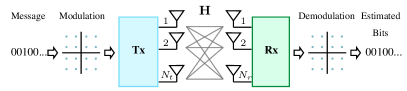
Figure 1: High-level system model of MIMO wireless communications. In this paper, we consider $N_{t}=N_{r}=2$.

Figure 2: The proposed complex DAE architecture with SVD. $\mathbf{v}_{\gamma}$ contains the singular values of the channel matrices and it is given to both of the Tx DAE and Rx DAE.

II-B SVD and Water-Filling Algorithm

To exploit spatial multiplexing in MIMO systems, precoding and power allocation have been developed to eliminate the inter-channel interference at each antenna at the Rx and to increase the data rate. SVD-based precoding [14] which is the optimal precoding in a closed-loop MIMO system, designed by utilizing CSIT and CSIR. In this method, the channel ${\mathbf{H}}$ is decomposed as

$$\mathbf{H}=\mathbf{U}\mathbf{\Lambda}\mathbf{V}^{H},$$ (2)

where $\mathbf{U}$ and $\mathbf{V}$ are two unitary matrices and $\mathbf{\Lambda}$ is the diagonal matrix with the singular values of ${\mathbf{H}}$. The matrices $\mathbf{V}$ and $\mathbf{U}^{H}$ are applied as precoding and pre-processing matrices. Then we have the observation as

$$\tilde{\mathbf{y}}\triangleq\mathbf{U}^{H}\mathbf{y}=\mathbf{\Lambda\Sigma}\mathbf{s}+\mathbf{U}^{H}\mathbf{w},$$ (3)

where $\mathbf{s}$ is the symbol vector that each element is independent and identically distributed (i.i.d.) symbol, $\mathbf{x}\triangleq\mathbf{V}\mathbf{\Sigma}\mathbf{s}$ is the signal and also the result of power allocation and precoding, $\mathbf{\Sigma}$ is the power allocation matrix obtained by water-filling (WF) [14]. In this way, SVD precoding eliminates the interference at each antenna and converts the correlated MIMO into a set of parallel sub-channels whose gain is the singular value of the channel matrix and the square root of the power allocated.

III SVD-Embedded DAE

The proposed SVD-Embedded DAE, (named as SVD-DAE for simplifying), structure for point-to-point (P2P) MIMO is shown in Fig. 2. In general, the system contains five parts: bit input, Tx, channel, Rx, and bit output. The Tx includes AE and precoding which construct a transmitted signal. Rx includes pre-decoding and AE to decode the received signal.

III-A Input Design

The input of the SVD-DAE contains two parts. The first part is for the information to be transmitted–the $N_{s}$ bits. The second part, $\mathbf{v}_{\gamma}$, is a feature vector related to the channel state information (CSI). The details of the two parts are described below.

III-A1 Transmitted Information

We feed the network with a vector containing $N_{s}$ bits in each transmission. Each bit is represented by $\pm 1$. Two input structures are considered:

• Bit input: The bit vector $\mathbf{v}_{b}$ is sent to the Tx DAE directly. The number of elements in $\mathbf{v}_{b}$ is $N_{s}$, which means the number of bits in each transmission period. In each period we transmit one $\mathbf{v}_{b}$, all the bits are independent and identically distributed following Binomial distribution.

• One-hot input: The one-hot input has already been used in [4, 6]. However, typically, the information to be transmitted is in bits. In this case, the bit vector is initially converted to a one-hot vector $\mathbf{v}_{o}$ by Gray coding and then transmitted to the DAE. Essentially, the encoding could be done arbitrarily since the DAE does not affect the order of the one-hot vectors.

III-A2 CSI Feature

Besides the bits for transmission, another feature vector $\mathbf{v}_{\gamma}$ is added which contains the effect of channel matrix and noise power level. We define $\bm{\gamma}$ as the channel gain to noise ratio, where the $i$th element in $\bm{\gamma}$ for $i$th sub-channel as ${\gamma}_{i}\triangleq\frac{{\lambda}^{2}_{i}}{\sigma_{N}^{2}}$. Then, we define the feature vector as

$$\mathbf{v}_{\gamma}\triangleq S_{c}\left(0.2\times 10\log_{10}({\bm{\gamma}}+10^{-6})\right),$$ (4)

where $S_{c}(t)$ is the zero-centered Sigmoid function rectifying the ${\rm\gamma}$ in dB between $-1$ and $1$, the factor $0.2$ scales ${\rm\gamma}$ in dB, and $10^{-6}$ is used to prevent ${\rm\gamma}$ going to zero and $\log_{10}({\bm{\gamma}})$ to negative infinity.

To summarize, the bit input vector is composed as $\mathbf{v}_{I}=[\mathbf{v}_{b},\mathbf{v}_{\gamma}]$ containing $N_{s}+N_{t}$ values, whereas for one-hot input, $\mathbf{v}_{I}=[\mathbf{v}_{o},\mathbf{v}_{\gamma}]$, the size is $2^{N_{s}}+N_{t}$.

III-B Tx DAE Design

The encoder of the SVD-DAE consists of a fully-connected neural network (FCNN) with two shortcut connections [15]. The size of the input is equal to the length of $\mathbf{v}_{I}$ while the output size is $N_{t}$. Each of the five layers in the middle contains 32 hidden nodes. The shortcuts, also called the residual connections, are used to provide a direct connection from the output to the input, which enables to convey the gradient in back-propagation and reduce the difficulty in training [16].

III-C Tx Precoding Design

In the Tx Precoding part, we add one layer with non-trainable weights that will not be updated during the training process. The weights are set according to right-singular vectors of the channel matrix, which is the optimal precoding for P2P MIMO problem with an infinite alphabet. When the channel coefficients are obtained, the weights of the Tx Precoding layer are set as $\mathbf{W}_{\rm T}=\mathbf{V}$ given in (2). The bias in each layer is set to be zeros. Before the transmission, a normalization layer linearly adjusts the total power at the output of Tx Precoding. The power of the transmit signal is equal to $P$. In this paper, $P=20$W is fixed for all DAEs and every signal transmission (per-example).

III-D Channel and Noise

The channel is formed by a non-trainable layer between the Tx and Rx. The weight of the channel layer is the channel matrix, i.e., $\mathbf{W}_{\rm Ch}=\mathbf{H}$. White Gaussian noise is added after implementing the channel layer. For each sub-channel, the noise power is $\sigma_{N}^{2}$. Since the bandwidth of the streams on each antenna is equal to the sampling frequency, the noise power then equals the noise spectral density, $\sigma_{N}^{2}=N_{0}$. To measure the overall signal and noise level, we define SNR following [6] that

$${\rm SNR}=\frac{P}{N_{0}}=N_{s}\frac{E_{b}}{N_{0}},$$ (5)

where $E_{b}\triangleq\frac{P}{N_{s}}$ refers to the energy per bit. The influence of the channel is not accounted for in this definition.

III-E Rx Pre-processing Design

In this part, we add two layers with non-trainable weights and zero biases. The number of hidden nodes is $N_{t}$. The weights in the first layer are $\mathbf{W}_{\rm R1}=\mathbf{U}^{H}$, where $\mathbf{U}^{H}$ is given in (2) and is left-singular vectors of the channel coefficients. Since $\mathbf{U}^{H}$ is a unitary matrix and we assume the noise on each receiving antenna has the same power, $\mathbf{U}^{H}\mathbf{w}$ has the same power as $\mathbf{w}$. So the noise level is not changed. Together with the Tx Precoding, an equivalent parallel channel can be obtained from the input of Tx DAE to the output of Rx DAE. The second layer in Rx Pre-processing unifies the diagonals to 1, whose weights are the pseudo-inverse of $\mathbf{\Lambda}$, i.e., $\mathbf{W}_{\rm R2}={\rm pinv}(\mathbf{\Lambda})$.

III-F Rx DAE Design

The input of Rx DAE contains the output of Rx Pre-processing and SNR feature, i.e., $\mathbf{v}_{\gamma}$ given in (4). The network structure, number of hidden layers, and nodes in each layer are the same as those in Tx DAE. The number of Rx DAE output varies according to the input design in Section III-A. When using bit inputs, the output size is $N_{s}$. Finally, the outputs are converted to bit vector $\hat{\mathbf{v}}_{b}$ and the BER for one transmitted vector is

$$\epsilon_{b}=\frac{1}{N_{s}}\sum_{\hat{\mathbf{v}}_{b}(j)\neq\mathbf{v}_{b}(j)}1.$$ (6)

For one-hot inputs, the output size is $2^{N_{s}}$. The output $\hat{\mathbf{v}}_{o}$s are firstly demodulated using Gray code. Then we calculate BER in a similar way as (6).

The loss function for bit input and one-hot input are mean-square error (MSE) and cross-entropy respectively. In general, cross-entropy is more efficient for training since a high loss value can be obtained on errors. However, it can only work for one-hot, a classification-like output. On the contrary, MSE is suitable for both regression and classification, while the cross-entropy is limited.

TABLE I: Parameters of the proposed DAE

Name	Hidden	If the weights are trainable
	layers$\times$nodes	and the weights (if not)
Tx Precoding	$1\times N_{t}$	N, $\mathbf{W}_{\rm T}=\mathbf{V}$, $\mathbf{b}_{\rm T}=\mathbf{0}$
Channel	$1\times N_{t}$	N, $\mathbf{W}_{\rm Ch}=\mathbf{H}$, $\mathbf{b}_{\rm Ch}=\mathbf{0}$
Rx Pre-processing	$1\times N_{t}$	N, $\mathbf{W}_{\rm R1}=\mathbf{U}^{H}$, $\mathbf{b}_{\rm R1}=\mathbf{0}$
	$1\times N_{t}$	N, $\mathbf{W}_{\rm R2}={\rm pinv}(\mathbf{\Lambda})$, $\mathbf{b}_{\rm R2}=\mathbf{0}$

The parameters of the proposed DAE are summarized in Table I. The main difference of the proposed DAE with the existing architecture in [6] is the two new blocks: Tx Precoding appended after Tx DAE and Rx Pre-processing before Rx DAE. The precoding and pre-processing introduced in this design is the optimal solution, SVD, for P2P MIMO precoding with the infinite alphabet [17]. We name the proposed architecture SVD-embedded DAE and use the shortened name SVD-DAE. If the SVD precoder and pre-processing are excludes, i.e., if we let $\mathbf{W}_{\rm T}=\mathbf{W}_{\rm R1}=\mathbf{W}_{\rm R2}=\mathbf{I}$, then we call it plain-DAE.

IV Training Process

In the training session, we first randomly generate $M_{c}$ channel matrices whose elements follow i.i.d. complex Gaussian distribution $\mathcal{CN}(0,1)$. In this paper, we consider $P=20$W and $N_{s}\in\{1,2,4,6\}$ bits. For each $N_{s}$, we have a different DAE instance which is trained with a stochastic strategy:

• We first train the DAE with the first channel and the batch size is $M_{b}$.

• In each batch, $N_{0}$ is uniformly and randomly chosen from $-20$dB to $25$dB. Both channel and $N_{0}$ are fixed.

• After applying the weights using Adam optimizer, we train the DAE with the next channel and another $N_{0}$.

• We continue until all $M_{c}$ channels are involved in the training, and the first round of training is finished.

• Next, the learning rate $l_{r}$ is reduced by a factor $\alpha_{r}$ and DAE goes to the next round of training.

The weights of the DAE are updated once per channel, and the loss of the DAE is expected to reduce to fit the channel. By repeatedly traversing all the channels, the DAE is trained in a stochastic manner. Theoretically, the DAE will adapt to an arbitrary channel if $M_{c}$ goes to infinity and traverses all possible channel matrices. In this paper, we set $M_{c}=2000$ and the number of rounds is $M_{r}=1000$.

The training approach is summarized in Algorithm 1. The detailed $E_{b}/N_{0}$ regions in the training stage are given in Table II. In the test stage, the DAEs are evaluated over $[-10,20]$dB.

Algorithm 1 Training Procedure

1:Select $N_{s}$, the number of bits in each transmission.

2:Set $M_{c}=2000$, $M_{b}=2000$, and $M_{r}=1000$;

3:Set $l_{r}=10^{-4}$, $\alpha_{r}=0.995$, and $P=20$W;

4:Initialize the DAE network.

5:for index $m_{r}$ from $1$ to $M_{r}$ do

6:     for index $m_{c}$ from $1$ to $M_{c}$ do

7:         Randomly and uniformly set $N_{0}$ in $[-20,25]$dB;

8:         Calculate and set the weights and biases in DAE

9:            according to Table I;

10:         Randomly generate $M_{b}$ bit vectors. Each bit fol-

11:            lows Binomial distribution with probability

12:            $P_{b}=0.5$;

13:         Train the DAE once with batch-size $M_{b}$;

14:     end for

15:     Update: $l_{r}=\alpha_{r}l_{r}$;

16:end for

TABLE II: SNR and $E_{b}/N_{0}$ region during the training according to (5). $N_{0}$ is uniformly distributed.

$N_{s}$	$P$ (W)	$N_{0}$ (dB)	SNR (dB)	$E_{b}/N_{0}$ (dB)
1	20	[-20, 25]	[-12,33]	[-12, 33]
2	20	[-20, 25]	[-12,33]	[-15, 30]
4	20	[-20, 25]	[-12,33]	[-18, 27]
6	20	[-20, 25]	[-12,33]	[-20, 25]

(a) $N_{s}$=1

(b) $N_{s}$=2

(c) $N_{s}$=4

(d) $N_{s}$=6

Figure 3: BER comparison between SVD-DAE and plain-DAE. The top x-axis denotes the SNR (dB) and the bottom x-axis denotes the $E_{b}/N_{0}$ (dB), where the relation is shown in (5). All the DAEs have residual connections as in Fig. 2.

V Numerical Results

V-A Performance of SVD in DAE

We first examine the performance of having the two new blocks, Tx Precoding and Rx Pre-processing, in the DAE. We plot the BER versus $E_{b}/N_{0}$ and SNR in each figure. The horizontal axis on the bottom of each figure and SNR is on the top. The relation between SNR and $E_{b}/N_{0}$ is given in (5). For each $E_{b}/N_{0}$, all the neural networks are tested and average over 2000 randomly generated channels.

The results in Fig. 3 show the comparison between SVD-DAE and plain-DAE. The plain-DAE has the same design as in Fig. 2 excluding the precoding and pre-processing parts. Besides, the extra feature vector for the plain-DAE becomes a vector with the real and imaginary parts of the channel matrix. We also plot the curves for the SVD with bit allocation as a baseline. Similar to [5, 4] we all have parallel sub-channels. The difference is we choose the best modulation schemes among BPSK and $M$-quadrature amplitude modulation ($M$-QAM) to reach the minimum BER over all of the sub-channels while the total bits transmitted is $N_{s}$. For the baselines, we limit the average power to $P=20$W. The peak power can be larger than $P$ when using $M$-QAM with $M>4$.

In general, SVD-DAE outperforms plain-DAE, that is, the solid lines are lower than the dotted lines in Fig 3. With $N_{s}$ increasing from Fig. 3(a) to Fig. 3(d), the benefit of SVD-DAE compared with plain-DAE is largely enhanced. For example, the BER reduces 30 times when $N_{s}=6$ and $E_{b}/N_{0}=10$dB but 10 times when $N_{s}=1$ and $E_{b}/N_{0}=10$dB. On the other hand, when transmitting fewer bits, the BER is smaller. For instance, when SNR is equal to 10dB, the BER of SVD-DAE in Fig. 3(a) is $10^{-5}$, while in Fig. 3(c) and Fig. 3(d), the BER is $7\times 10^{-4}$ and $6\times 10^{-3}$, respectively. SVD-DAE outperforms the baseline from 1.5 to 18 times on BER improvement.

The bit input is better than one-hot input for low SNRs. The curves with circle markers in Fig. 3(b), Fig. 3(c), and Fig. 3(d) are lower than the curves with triangles. This is because, when using one-hot input, DAE cannot optimize the bit-to-symbol conversion which is outside the DAE and is fixed by using Gray code. Putting it differently, the bit labeling (bit-to-symbol mapping) is invisible using the one-hot method. However, if we use bit inputs, the bit labeling can be optimized in the training. Besides, in Fig. 3(d), when SNR is greater than 10dB, the SVD-DAE with one-hot input performs better than the bit input. That is, the advantage of cross-entropy loss appears in one-hot input. Also, if we aim at optimizing the SER, one-hot input will always be better than the bit input (for saving space, we omit that result). In Fig. 3(a), SNR and ${E_{b}}/{N_{0}}$ are the same and the 1-bit input and one-hot input achieve similar performance. This is because one-hot input has no BER loss in the bit-to-symbol conversion when the input carries only one bit of information ($N_{s}=1$).

Figure 4: Performance of residual connections on plain-DAE when $N_{s}$=4.

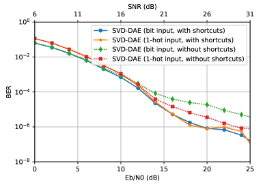
Figure 5: Performance of residual connections on SVD-DAE when $N_{s}$=4.

Figure 6: SVD-DAE compared with SVD-WF-DAE on BER when $N_{b}$=4.

V-B The Effect of Residual Connections in DAE

We study the effect of adding a residual connection, i.e., shortcuts, which enables to convey the gradient in back-propagation and reduce the difficulty in training by providing a direct connection from the output to the input. We apply the shortcuts to both plain-DAE and SVD-DAE, $N_{s}$ is chosen to be 4 for this experiment. In Fig. 4 and Fig. 5, the BER is greatly reduced in both networks with the shortcuts compared with having no shortcuts, especially when $E_{b}/N_{0}$ is greater than 10dB. It reduces the BER of plain-DAE with bit input from $3\times 10^{-2}$ to $10^{-3}$ when $E_{b}/N_{0}=20$dB (Fig. 4). For SVD-DAE with bit inputs, the BER is improved from $2\times 10^{-5}$ to $0.9\times 10^{-6}$ (Fig. 5).

V-C The Effect of Adding WF

The SVD with water-filling algorithm (WF) is known to be optimal precoding in the MIMO system to achieve spatial multiplexing [14]. This encouraged us to add WF as a non-trainable layer to the SVD-DAE. The power allocation factors given by WF can amplify or attenuate the output of the Tx-DAE depending on the value greater or less than $1$. The power normalization in the Tx Precoding block is also effective. However, WF is not the optimal power allocation scheme in finite-alphabet MIMO systems [18]. This could be the reason why SVD-DAE without WF performs better than SVD-DAE with WF (see in Fig. 6). One explanation can be that the WF algorithm allocates all the power to the stronger channel at low SNR ($E_{b}/N_{0}\leq 10$dB) which results in a good BER performance. However, when SNR increases, WF starts assigning more power to strong channels and less power to weaker channels, in which the poor channel may not make use of the power and then suffers a bad BER. In SVD-DAE, the singular values and noise level are fed to the Tx and Rx DAEs. Such a design is inspired by WF and allows the AE networks to learn their own WF-like solution to distribute information across channels.

VI Conclusions

We have improved the existing DAE for MIMO systems by introducing SVD as a differentiable layer in the network. This helps DAE make better use of the inputs of Tx autoencoder to eliminate the interference and improve the performance of MIMO spatial multiplexing. SVD-DAE can outperform plain-DAE, and is competitive with linear precoding solutions in terms of BER. We have also investigated the ability of the proposed DAE with bit inputs and one-hot inputs. Based on our results, bit input is a good candidate for DAE especially in reducing the BER. By tuning the network, residual connections are added to increase the depth of the network and further improve the results. Besides, it is meaningful to investigate different constraints such as per-channel, per-antenna, per-sum-of-antennas average power constraints in the future.

References

- [1] T. O’Shea and J. Hoydis, “An introduction to deep learning for the physical layer,” IEEE Transactions on Cognitive Communications and Networking, vol. 3, no. 4, pp. 563–575, 2017.
- [2] S. Dörner et al., “Deep learning based communication over the air,” IEEE Journal of Selected Topics in Signal Processing, vol. 12, no. 1, pp. 132–143, 2017.
- [3] H. Ye et al., “Deep learning-based end-to-end wireless communication systems with conditional GANs as unknown channels,” IEEE Transactions on Wireless Communications, vol. 19, no. 5, pp. 3133–3143, 2020.
- [4] T. J. O’Shea et al., “Deep learning based MIMO communications,” arXiv:1707.07980, 2017.
- [5] D. Tse and P. Viswanath, Fundamentals of wireless communication. Cambridge, U.K.: Cambridge university press, 2005.
- [6] J. Song et al., “Benchmarking end-to-end learning of MIMO physical-layer communication,” in Proc. IEEE Global Communications Conference (GLOBECOM), 2020, pp. 1–6.
- [7] N. Farsad et al., “Deep learning for joint source-channel coding of text,” in Proc. IEEE International Conference on Acoustics, Speech and Signal Processing (ICASSP), 2018, pp. 2326–2330.
- [8] H. Ye et al., “Channel agnostic end-to-end learning based communication systems with conditional GAN,” in Proc. IEEE Global Communications Conference (GLOBECOM) Workshops, 2018, pp. 1–5.
- [9] X. Zhang and M. Vaezi, “Multi-objective DNN-based precoder for MIMO communications,” IEEE Transactions on Communications, vol. 69, no. 7, pp. 4476–4488, 2021.
- [10] J. Shi et al., “Deep learning based robust precoding for massive MIMO,” IEEE Transactions on Communications, 2021.
- [11] C.-K. Wen et al., “Deep learning for massive MIMO CSI feedback,” IEEE Wireless Communications Letters, vol. 7, no. 5, pp. 748–751, 2018.
- [12] A. Felix et al., “OFDM-autoencoder for end-to-end learning of communications systems,” in Proc. of IEEE International Workshop on Signal Processing Advances in Wireless Communications (SPAWC), 2018, pp. 1–5.
- [13] Y. Jiang et al., “Turbo autoencoder: Deep learning based channel codes for point-to-point communication channels,” Advances in Neural Information Processing Systems, vol. 32, pp. 2758–2768, 2019.
- [14] T. M. Cover and J. A. Thomas, Elements of information theory. 2th ed. NJ, USA: Wiley, 2006.
- [15] S. R. K. He, X. Zhang and J. Sun, “Deep residual learning for image recognition,” Computing Research Repository (CoRR), 2015.
- [16] D. J. Ji et al., “Convae: A new channel autoencoder based on convolutional layers and residual connections,” IEEE Communications Letters, vol. 23, no. 10, pp. 1769–1772, 2019.
- [17] E. Telatar, “Capacity of multi-antenna Gaussian channels,” European Transactions on Telecommunications, vol. 10, no. 6, pp. 585–595, 1999.
- [18] C. Xiao et al., “Globally optimal linear precoders for finite alphabet signals over complex vector Gaussian channels,” IEEE Transactions on Signal Processing, vol. 59, no. 7, pp. 3301–3314, 2011.